The Effect of Skill Shortages on Unemployment and …repec.org/res2003/Wallis.pdf1 The Effect of...

1

The Effect of Skill Shortages on

Unemployment and Real Wage Growth: A

Simultaneous Equation Approach

Gavin Wallis

[email protected]

Office for National Statistics

August 2002

Abstract

This paper attempts to quantify the effect of skill shortages on the UK labour market by

developing a simultaneous equation model of unemployment and real wage growth. The

model is developed following a structural approach based on a priori economic

information and is initially estimated using a two-stage least squares procedure. The

model is also estimated using Zellner’s seemingly unrelated regressions estimation

technique, with similar results. It is shown that skill shortages have a positive effect on

real wage growth and a negative effect on unemployment, with both these effects

economically and statistically significant.

JEL classifications: C32, C51, C52, E24

Keywords: Skill Shortages, Unemployment, Wages, 2SLS

2

1. Introduction

Academic and vocational qualifications are commonly used as a proxy for skills when

assessing the personal and social returns of training and education and the level of skills in

a country. The use of qualifications as a proxy for skills is a useful and objective way of

measuring an individual’s skill base but it does have its limitations when looking at the

implications of skill levels on the UK economy. The UK has experienced a major shift in

its occupational structure in the past 20 to 30 years, with a corresponding shift in the

demand for skills. The demand for generic skills such as communication and problem

solving has increased whilst the demand for skills relating to manual occupations has

declined. Qualifications, although being a relatively good indicator of the supply of skills,

do not provide a measure of the demand for skills. More emphasis needs to be put on

identifying the skill needs and shortages that exist in the UK.

The need has been recognised. In 1998 the Secretary of State for Education and

Employment established the Skills Task Force (STF), set up to help develop a National

Skills Agenda by providing evidence on skill needs and shortages in the UK. A Research

Programme was also set up under the direction of Terence Hogarth and Rob Wilson at the

Institute for Employment Research (IER), at the University of Warwick, in order to

“provide evidence on the nature, extent and pattern of skill needs and shortages and their

likely future development”1. A major part of this research included two Employer Skill

Surveys (ESS), carried out in 1999 and 2001, aimed at providing a comprehensive

analysis of skill deficiencies in the UK 2. The research programme also included a review

of existing surveys, including those by the Confederation of British Industries (CBI) and

the British Chambers of Commerce (BCC).

In a recent Labour Market Trends article it was noted, “there has been increasing media

reporting of skills shortages and their possible implications within the UK economy”3.

The aim of this paper is to quantify the effect of skill shortages on unemployment and real

wage growth in the UK by developing a simultaneous equation model. This model will

1 See foreword of Bosworth et al [6].2 These surveys were undertaken by IFF Research and the IER.3 See [14]. This article also provides a good overview of the current extent of skill shortages in the UK.

3

include a measure of skill shortages, which will be taken from the CBI’s Industrial Trends

Survey. The effect of skill shortages on real wage growth and unemployment can then be

assessed.

Section 2 provides background information and comparisons of the various measures of

skill shortages that are available to the researcher, introducing the CBI and BCC surveys

and the Employer Skill Surveys. I will also discuss the reasoning behind choosing the

CBI survey for my regression analysis. Section 3 will introduce the model used to

quantify the effect of skill shortages on real wage growth and unemployment. I will also

discuss the economic rational behind the model and the structural approach that I have

followed.

Section 4 introduces the variables I am using in my model, with some summary statistics

and a priori observations of the data, and Section 5 discusses my estimation and sample

period. Section 6 presents the basic result of the two-stage least squares estimation of my

real wage growth and unemployment equations, with model evaluation and diagnostics in

section 7. Section 8 builds on sections 6 and 7 by introducing an alternate estimation

technique, seemingly unrelated regressions, and comparing the results with the two-stage

least squares estimation. The implications of my equations and the link between skill

shortages and unemployment are discussed in sections 9 and 10, respectively. Section 11

outlines possible directions of future research and section 12 concludes.

2. Background

2.1. Skill Shortages and Skill Surveys

There are three main skill surveys conducted in the UK that provide information on the

level of skill shortages. Theses are the Employer Skills Survey, the CBI Industrial Trends

Survey, and the BCC Quarterly Economic Survey. The problem that arises for a

researcher is that these surveys are not based on the same measurement of skill shortages.

The DfEE research into existing survey evidence on skill deficiencies noted that, “The

interpretation of these surveys is bedevilled by differences in methodology, terminology,

4

and phraseology”. Caution must therefore be taken when comparing the results of these

surveys.

The Department for Education and Skills (DfES, formerly Department for Education and

Employment) defines skill shortages vacancies as a “A situation where there is a genuine

shortage in the accessible external labour market of the type of skill being sought, and

which leads to a difficulty in recruitment”. Skill shortage vacancies are thus vacancies

explicitly attributed to a lack of job applicants with the required skills, qualifications or

work experience. This is only one possible definition of skill shortages and other sources

use different definitions, or measure different things when trying to quantify skill

shortages.

The DfES also identifies internal skill gaps, which reflects a situation where employees’

current skills are insufficient to meet the business objectives of the employer. One

problem that arises is that some surveys count this type of skill gap and others do not. In

the Employer Skill Surveys this measure of skill shortage is separated from other types of

skill shortages. In the CBI survey only one measure of skill shortages is recorded and this

includes internal skill gaps. The BCC survey measure of skill shortages does not consider

internal skill gaps, focusing solely on recruitment difficulties. It is clear then that caution

must be taken when comparing the three surveys4.

A problem that all three of the surveys suffer from is the idea of latent skill gaps. The

DfES identifies two types of latent skill gaps that can occur and hence bias survey data,

Latent skills gaps can take two main forms. First, for a variety of reasons, employers may fail to

report some problems. This may be because the respondent is unaware that they exist or they may

choose not to report vacancies (for instance, if they feel that there is no hope of filling them).

Second, and potentially much more important, respondents may simply not perceive that they have

a problem, because they are not fully aware of skills that might be needed to optimise their

company’s performance.

4 In section 2.4. I will attempt to provide some comparison of the three surveys considering the different

measures adopted of measuring skill shortages.

5

Both types of latent skill gaps identified above will lead to employers understating the

level of skill shortages5, thus survey results will tends to understate the true level of skill

shortages. Bosworth et al [7] assess the importance of latent skill gaps using the 1999

Employer Skill Survey. The econometric analysis suggests that establishment’s

perceptions of their skill needs are linked to their strategies and their success. Their Key

finding regarding latent skill gaps is that “enterprises that adopted new working practices

were, on average, much more likely to report lower levels of proficiency amongst their

workforce and that those that had adopted new technologies or new products were likely

to be significantly more satisfied with the quality of their employees”. They conclude

that, “the incidence of both internal skill gaps and external recruitment difficulties would

rise significantly for such establishments were they to be transformed by raising their

aspirations and improving their performance. The intensity of reported external

recruitment problems would increase sharply as well, especially for skill shortage

vacancies”. 6

2.2. Employer Skill Surveys

The DfES undertook surveys of the Skill Needs in Britain (SNB) on an annual basis

between 1990 and 1998 in order to provide a snap shot of skill needs at the time of each

survey. Although these surveys proved useful, the two Employer Skill Surveys (ESS)

conducted in 1999 and 2001 were of a much larger scale and were undertaken as part of a

comprehensive analysis of skill deficiencies. The aim of the surveys was to identify the

incident, causes and implications of skill deficiencies reported by employers.

The ESS 1999 surveyed establishments employing five or more employees with a

repressive sample being drawn from all sectors except agriculture. The survey consisted

of 23,070 telephone interviews and 3,882 face-to-face interviews. The ESS 2001

surveyed establishments with one or more employee and included all sectors. The survey

5 The first type of skill gap is essential not a latent skill gap but a consequence of measurement error. The

second type is simply not recognised and so is a true latent skill gap.6 See Bosworth et al [7] and also ‘News and Research – DfES News’ in Labour Market Trends, Volume

110, January 2002, Pg. 8.

6

consisted of 27,031 telephone interviews7. The scale of the two surveys makes them the

most representative and comprehensive surveys of skill shortages in the UK. Care has to

be taken however when comparing the results of these two surveys as the shift in the

sample had a significant impact on the survey results, this is allowed for in the ESS 2001

statistical report8.

The Employer Skill Surveys investigate two different kinds of skill deficiencies, these are,

• external recruitment difficulties, focusing in particular on hard-to-fill vacancies and what are

referred to as skill-shortage vacancies, (hard-to-fill vacancies explicitly attributed to a lack of

job applicants with the required skills, qualifications or work experience)

• internal skill gaps (defined as occurring where a significant proportion of existing staff in a

particular occupation are not fully proficient at their current jobs).

The Employer Skills Survey Statistical Reports, [6] and [21], present the survey results on

vacancies, hard-to-fill vacancies, skill-shortage vacancies and internal skill gaps in various

breakdowns, including by sector, occupation, region and establishment size. For my

purposes the aggregate level of these measures is most important.

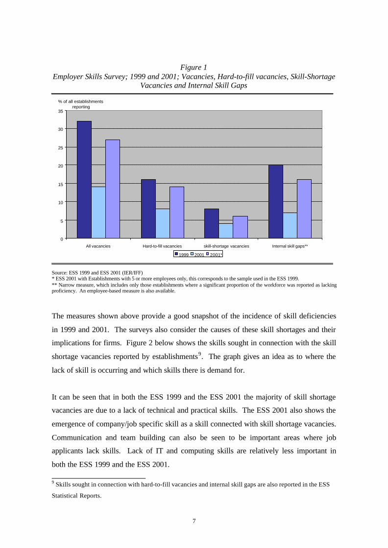
Figure 1 below shows the overall percentage of establishments reporting the three

measures of vacancies and internal skill gaps in the two surveys and also the results from

the reduced 2001 sample, which corresponds to the sample used in the ESS 1999. It can

be seen that the all the measures of skill deficiencies have fallen in 2001 compared to

1999, even if the reduced 2001 sample is used. The effect of reducing the sample can be

seen to have a large affect on the results.

7 In comparison the last Skill Needs in Britain survey consisted of 4,000 telephone interviews. See the

technical appendix of Hogarth et al [21] for further technical detail on this survey.8 See Hogarth et al [21].

7

Figure 1Employer Skills Survey; 1999 and 2001; Vacancies, Hard-to-fill vacancies, Skill-Shortage

Vacancies and Internal Skill Gaps

Source: ESS 1999 and ESS 2001 (IER/IFF)* ESS 2001 with Establishments with 5 or more employees only, this corresponds to the sample used in the ESS 1999.** Narrow measure, which includes only those establishments where a significant proportion of the workforce was reported as lackingproficiency. An employee-based measure is also available.

The measures shown above provide a good snapshot of the incidence of skill deficiencies

in 1999 and 2001. The surveys also consider the causes of these skill shortages and their

implications for firms. Figure 2 below shows the skills sought in connection with the skill

shortage vacancies reported by establishments9. The graph gives an idea as to where the

lack of skill is occurring and which skills there is demand for.

It can be seen that in both the ESS 1999 and the ESS 2001 the majority of skill shortage

vacancies are due to a lack of technical and practical skills. The ESS 2001 also shows the

emergence of company/job specific skill as a skill connected with skill shortage vacancies.

Communication and team building can also be seen to be important areas where job

applicants lack skills. Lack of IT and computing skills are relatively less important in

both the ESS 1999 and the ESS 2001.

9 Skills sought in connection with hard-to-fill vacancies and internal skill gaps are also reported in the ESS

Statistical Reports.

0

5

10

15

20

25

30

35

All vacancies Hard-to-fill vacancies skill-shortage vacancies Internal skill gaps**

% of all establishments reporting

1999 2001 2001*

8

Figure 2ESS 1999 and 2001; Skills Sought in Connection with Skill-Shortage Vacancies

Base: All Skill shortage vacanciesSource: ESS 2001 Statistical Report (IER/IFF). ESS 1999 and ESS 2001.

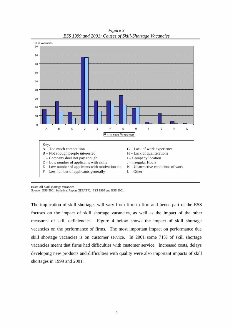
Figure 3 below shows the causes of skill shortage vacancies as identified by employers. A

low number of applicants with skills can be seen as the main cause of skill shortage

vacancies with figures for both the ESS 1999 and ESS 2001 close to 80%. The second

most important cause of skill shortage vacancies is a lack of work experience.

Interestingly a lack of qualifications is the causes of only around 20% of vacancies, lack

of skills is a much bigger cause of skill shortage vacancies. Factors such as pay and

location are not significant causes of skill shortage vacancies.

0

5

10

15

20

25

30

35

40

45

50

% of vacancies

ESS 1999 ESS 2001

9

Figure 3ESS 1999 and 2001; Causes of Skill-Shortage Vacancies


The implication of skill shortages will vary from firm to firm and hence part of the ESS

focuses on the impact of skill shortage vacancies, as well as the impact of the other

measures of skill deficiencies. Figure 4 below shows the impact of skill shortage

vacancies on the performance of firms. The most important impact on performance due

skill shortage vacancies is on customer service. In 2001 some 71% of skill shortage

vacancies meant that firms had difficulties with customer service. Increased costs, delays

developing new products and difficulties with quality were also important impacts of skill

shortages in 1999 and 2001.

0

10

20

30

40

50

60

70

80

90

A B C D E F G H I J K L

% of vacancies

ESS 1999 ESS 2001

Key:A – Too much competition G – Lack of work experienceB – Not enough people interested H – Lack of qualificationsC – Company does not pay enough I – Company locationD – Low number of applicants with skills J – Irregular HoursE – Low number of applicants with motivation etc. K – Unattractive conditions of workF – Low number of applicants generally L – Other

10

Figure 4ESS 1999 and 2001; Impact of Skill-Shortage Vacancies on Performance


The graph also show that skill shortages vacancies are having a greater impact in all areas

of performance, except loss of orders and needing to withdraw products, in 2001 than in

1999. Establishments in the survey were also asked what solutions have been adopted to

combat skill shortage vacancies and skill gaps. Common solutions to skill shortages

included increased salaries and increased training. Some 80% of establishments provided

further training as a solution to skill gaps with relocating work within the company an

increasingly common response.

The data presented above provides only a small sample of the wide range of data available

from the Employer Skill Surveys10. The surveys also highlight the importance of regional

and sectoral differences in the incidence of hard-to-fill vacancies, skill shortage vacancies

10 The reader is referred the Employer Skill Survey Statistical Reports, [6] and [21], for a full summary and

analysis of the Survey results.

0

10

20

30

40

50

60

70

80

A B C D E F G H

% of skill-shortage vacancies

ESS1999 ESS2001

Key:A – Loss of orders E – Difficulties with qualityB – Delays developing new products F – Increases costsC – Withdraw products G – Difficulties with technological changeD – Difficulties with new customers H – Difficulties with organisational change

11

and skill gaps. These differences could have implications when estimating aggregate

wage and unemployment equations.

Due to their large sample size and representative coverage the Employer Skill Surveys can

be regarded as the most comprehensive surveys of skill shortages in the UK. Their only

problem lies in the fact that they only represent two points in time and so say little about

changes in the level of skill shortages over time. Hence, they cannot be used for time

series regression analysis.

2.3. CBI Industrial Trends Survey

The CBI industrial Trends Survey (ITS) was first introduced in 1958, when it was

published three times a year, and covers only manufacturing firms in the UK. Since 1972

it has been conducted on a quarterly basis, with the most recent survey being July 2002.

The survey results are disaggregated by four employment size groups, three market

sectors, twelve broad industrial sectors and 50 individual industries. The total sample

(UK) data is weighted according to industrial sector, net output and employment size to

give a representative sample of the UK. The most recent sample covers over 1500 UK

firms and is currently conducted by post. The sample has been criticised for being more

representative of larger employing firms but this is allowed for in weighting the results.

The survey asks firms a range of questions but the one that is directly relevant to skill

shortages is question 14 of the survey, which is:

What factors are likely to limit your output over the next four months? Please tick the

most important factor or factors. If you tick more than one factor it would be helpful if

you could rank them in order of importance.

a) Orders or Sales

b) Skilled Labour

c) Other Labour

d) Plant Capacity

e) Credit or Finance

f) Materials or Components

g) Other

12

The proportion of respondents identifying skilled labour as a factor limiting output can

then be used as a measure of skill shortages. Figure 5 below shows the CBI survey data

for the period 1972 to 2001. The graph shows the proportion of respondents identifying,

orders or sales, skilled labour, and other labour as factors limiting output. It is clear than

the majority of firms in the survey identified orders or sales as the main factor limiting

output, except for a period in 1973-74 when skilled labour became a more important

factor.

Figure 5CBI ITS: Proportion of Respondents Identifying each Factor as Main Factor Limiting

Output; UK; 1972 to 2001, not seasonally adjusted

Source: CBI Quarterly Industrial Trends Survey

The skilled labour time series above can be used as a measure of skill shortages and

provides a good length time series for regression analysis. The data from the survey is

also generally regarded as representative; see Hart [17], Rosewell [30], or Blake et al

[5].11

11 Haskel and Martin [18] use the CBI skill shortages data to test the effect of skill shortages on Productivity.

0

10

20

30

40

50

60

70

80

90

100

1972 1974 1976 1978 1980 1982 1984 1986 1988 1990 1992 1994 1996 1998 2000

Per cent

Orders or sales Skilled labour Other labour

13

2.4. BCC Quarterly Economic Survey

The BCC Quarterly Economic Survey covers both manufacturing and service sector firms

and has been running since 1985. The 2001 Q4 survey covered 7182 companies

employing 900,000 people, 2556 manufacturing firms responded employing 297,779

people and 4626 service sector firms employing 618,224 people. Since 1989 total

responses have been weighted according to the actual distribution of companies by size

within the UK to try to ensure representative results, before this results were neither

representative of all UK regions nor weighted. Due to the size of the survey it is

considered the most representative of its kind in the UK 12.

The survey questions most relevant to skill shortages are the following,

BCC7a. Have you attempted to recruit staff over the past 3 months?

Yes/No

BCC7c. Did you experience any recruitment difficulties finding suitable staff?

Yes/No

BCC7d. If yes, for which of the Following categories?

a) Skilled manual and technical

b) Professional and managerial

c) Clerical

d) Unskilled and semi-skilled labour

Question BCC7c. is the main skill shortages measure, with question BCC7d. giving

information as to the type of skills that are required for the recruitment difficulties

reported. The proportion of respondents identifying recruitment difficulties can be used as

a measure of skill shortages and the resultant time series can be used to look at the path of

skill shortages over time. Figure 6 below shows the BCC survey data for the period 1988

12 The DfES warns that the survey has increased significantly over time. See Blake et al [5].

14

Q4 to 2001 Q4 for question BCC7c, showing the proportion of respondents identifying

recruitment difficulties in both the manufacturing and service sectors.

Figure 6BCC Quarterly Economic Survey; Proportion of Firms Identifying Recruitment

Difficulties; UK; 1988 Q4 to 2001 Q4, not seasonally adjusted (NSA)

Source: BCC Quarterly Economic Survey

Using the BCC series as a measure of skill shortages it can be seen that over the period

1988 to 1991 there was a sharp decline in the level of skill shortages. Since then there has

been a steady upward trend in skill shortages until around 1997, with skill shortages

remaining at about the same level since then. This is the same for both the manufacturing

and service sector, with the two series moving together for the whole period, but with

manufacturing skill shortages generally slightly higher.

The BCC data gives some indication of the changes in skill shortages over time. The

series is however only representative since 1989 and so provides only a limited period of

time series data compared to the CBI data. The use of recruitment difficulties as a

measure for skill shortages is also questionable, the ESS discussed above makes a

distinction between recruitment difficulties (hard-to-fill vacancies) and skill-shortage

vacancies, and the surveys show that recruitment difficulties are generally much higher

than skill-shortage vacancies. Hence not all recruitment difficulties are due to skill

10

20

30

40

50

60

70

80

1988 Q4 1990 Q4 1992 Q4 1994 Q4 1996 Q4 1998 Q4 2000 Q4

BCC Survey percentage

BCC service sector BCC manufacturing sector

15

shortages and so the BCC data used as a measure of skill shortages is overestimating the

level of skill shortages13.

2.5. Comparisons and Regression Analysis

A comparison of the three surveys above can be somewhat misleading and care has to be

taken in doing so. Different methodologies and phraseologies mean that results cannot be

compared directly. Table 1 below shows a comparison of the three surveys and includes

an appropriate definition of the skill shortage measure being used in each survey.

Table 1Comparison of CBI Industrial Trends Survey, BCC Quarterly Economic Survey and the

Employer Skill Surveys; 1999 and 2001.

Source: ESS 1999 and ESS 2001 (IER/IFF); CBI Industrial Trends Survey; BCC Quarterly Economic SurveyNotes: CBI and BCC figures are taken from quarterly data and are averages for the year.* ESS 2001 with Establishments with 5 or more employees only, this corresponds to the sample used in the ESS 1999.** Narrow measure, which includes only those establishments where a significant proportion of the workforce was reported as lackingproficiency.

The CBI data is a measure of total skill shortages, whilst the ESS data has two measures

of skill shortages, skill-shortage vacancies and internal skill gaps. Comparing the CBI

data to the sum of the two ESS measures gives different pictures of skill shortages. Using

either of the two 2001 samples for the ESS, skill shortages in 2001 fell compared to 1999,

whilst the CBI data indicates an increase in skill shortages. The BCC data can only really

be compared to the ESS data for hard-to-fill vacancies in terms of absolute values14.

These two measures of recruitment difficulties also show different pictures, with the ESS

13 The BCC data may still provide a good measure of the time path of skill shortages.14 I will compare the trend of the BCC data with that of the CBI data later.

Survey Definition of skill shortage measure 1999 2001 2001*

ESS All vacancies 32 14 27

ESS Hard-to-fill vacancies 16 8 14

ESS skill-shortage vacancies 8 4 6

ESS Internal skill gaps** 20 7 16

CBI Shortage of skilled labour limiting output 9.5 15.75 -

BCC Services Recruitment Difficulties 62.5 64 -BCC Manufacturing Recruitment Difficulties 70 69.5 -

16

indicating reduced recruitment problems and the BCC indicating increased recruitment

problems in the service sector and slightly reduced recruitment problems in the

manufacturing sector.

One other problem in comparing the surveys is the nature of the questions. The ESS ask

about establishment current situation, the CBI question asks about the next 4 months, so is

essentially an estimate of future skill shortages, and the BCC survey asks about the

previous 3 months. The ESS data is also a snapshot of a specific point in time, whereas

the CBI and BCC are time series data. This leads to difficulties as to which CBI and BCC

measures to compare with the ESS data. Using the yearly average of the quarterly data as

I have done above may not be appropriate given the nature of the ESS data and the

variations in skill shortages that occur over the period of a year. These differences lead to

difficulties when comparing the results.

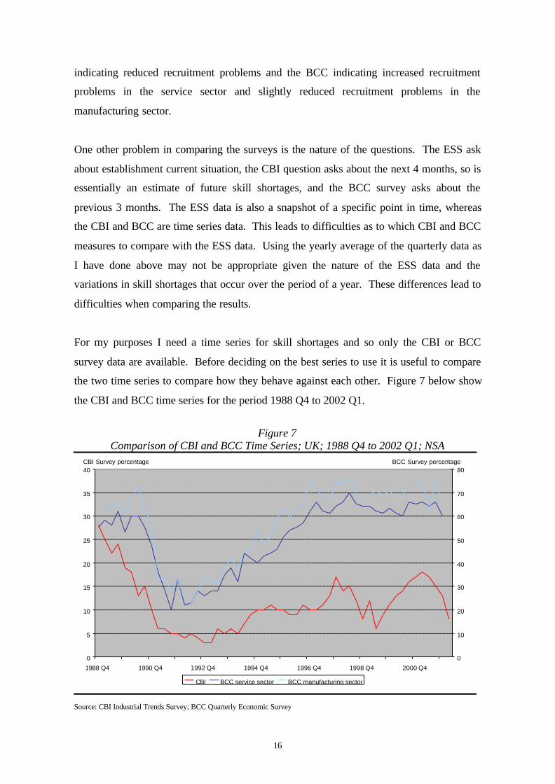
For my purposes I need a time series for skill shortages and so only the CBI or BCC

survey data are available. Before deciding on the best series to use it is useful to compare

the two time series to compare how they behave against each other. Figure 7 below show

the CBI and BCC time series for the period 1988 Q4 to 2002 Q1.

Figure 7Comparison of CBI and BCC Time Series; UK; 1988 Q4 to 2002 Q1; NSA

Source: CBI Industrial Trends Survey; BCC Quarterly Economic Survey

0

5

10

15

20

25

30

35

40

1988 Q4 1990 Q4 1992 Q4 1994 Q4 1996 Q4 1998 Q4 2000 Q4

CBI Survey percentage

0

10

20

30

40

50

60

70

80BCC Survey percentage

CBI BCC service sector BCC manufacturing sector

17

Figure 7 above shows that the CBI and BCC series exhibit similar behaviour over the

period even though their absolute level differ quite dramatically. The difference in

absolute level is due to the BCC data having a much wider definition of skill shortages

than the CBI. Both series show a decline between 1984 and 1992, followed by an increase

until about 1997. Since then the BCC data has been relatively stable with the CBI data

less stable, but still fluctuating around its 1997 value. The main difference in the series is

that the BCC data indicates that skill shortages in 2001 Q4 are above their 1988 level,

whilst the CBI data indicates that skill shortages are below their 1988 level.

For my time series analysis I will be using the CBI time series as opposed to the BCC time

series for a number of reasons. Firstly the CBI time series is a much longer series than the

BCC series. The BCC series is only representative of the UK since 1989; this would limit

my sample significantly. Given the finite sample properties of two-stage least squares a

larger sample is preferable.

The CBI series is also closer to the definition of skill shortages used by the DfES and in

the Employer Skill Surveys. The CBI series has tended to be consistent with the Skill

Needs in Britain surveys 15 and is generally regarded as representative of the UK.

Although the CBI survey data does not appear consistent with the ESS data (see table 1

above) the difficulties in making comparison should be considered. The CBI skill

shortage measure is of the same magnitude as the ESS data, unlike the BCC data, and so

although showing a slightly different picture between 1999 and 2001 is much more

consistent with the ESS.

3. The Model

3.1. The structural model

The model used to estimate the effect of skill shortages on unemployment and real wage

growth is based on the structural approach used by Manning (1993), Layard and Nickel

(1985) and discussed by Bean (1994). The model uses a priori economic information

15 See [12].

18

and is most closely based on a Phillips curve type relationship. The model specification

does however differ from the conventional approach in order to avoid the wage equation

being unidentified. In the conventional approach no variable is excluded from the wage

equation and so it is unidentified16. The model is estimated of the form:

( ) tttt uXUNPW 11210 +++=−∆ ααα

tttt uXPWUN 22210 )( ++−∆+= βββ

Where, ( )PW −∆ is the rate of change of real wages, UN is the unemployment rate, 1X is

a vector containing factors that affect real wage growth, 2X is a vector containing factors

that affect unemployment and u are stochastic disturbances.

The first equation is generally interpreted as a wage setting equation and the second

equation a labour demand curve or pricing equation. The conventional wage setting

equation includes variables such as union power and the replacement ratio. I did not want

to use data such as this due to limited availability and concentrated more on key indicators

of the macro economy.

One thing to notice about the equations above is that they do not contain a productivity

variable. In the theoretical foundations of the Phillips curve productivity does not play an

important role in structural wage equations, although it is important for the long run

growth of wages. As Manning notes, “this does not mean that productivity growth does

not cause the growth in real wages over time. But, suppose that the labour market was

competitive and that labour supply was totally inelastic. Then productivity growth leads

to real wage growth, but it would be strange to argue from this that one should include

productivity directly in the estimate of the structural labour supply curve”. Here we are

interested in the variability of real wage growth not the long-run growth.

16 The Issue of identification has become central to the wage determination literature. See Manning (1993)

and Bean (1994).

19

3.2. Final Specification

The final specification of the model was determined after testing various alternate

specifications and by removal of superfluous arguments in a stepwise fashion. The

alternate specifications that were tried did not perform as well and produced less robust

results. The final specification is as follows:

tttttt

ttttt

uGFCFGDPGrowthGDPGrowthGDPStockageSkillShort

ageSkillShortWGrowthWGrowthUNWGrowth

119187615

4431210

/ ++++++

++++=

−−−

−−

ααααα

ααααα

ttttttt urGDPGrowthUNUNWGrowthUN 2454431210 ++++++= −−− ββββββ

Where WGrowth is real wage growth, UN is the unemployment rate, SkillShortage is the

CBI’s measure of skill shortages, Stock/GDP is the stock (inventories) to Gross Domestic

Product ratio, GDPGrowth is the quarter on quarter yearly growth rate, GFCF is gross

fixed capital formation (millions), and r is the short-term interest rate. tu1 and tu2 are

stochastic disturbance terms.

3.3. Economic Rationale for Variables

The GDPGrowth variable is included to capture the general state of the economy and is

expected to have a positive effect on real wage growth and a negative effect on

unemployment. The GFCF and Stock/GDP variables are included to pick up the

importance of labour (and therefore influence wages) in firms output decisions. Prior

beliefs on the direction of these variables are less certain. An increased stock to GDP ratio

could give firms more wage bargaining power and so reduce wage growth but could also

result in increased wage growth due to the labour requirements of increasing inventories.

The appearance of the interest rate in the unemployment equation has no theoretical

foundation but has be found by many authors, including Manning [27], to be an important

determinant of unemployment in empirical studies. The interest rate variable is expected

to have a positive effect on unemployment.

20

The skill shortages variable is included for obvious reasons, as it is the effect of which we

are ultimately trying to measure. We would expect the variable to have a positive effect

on real wage growth, with increased skill shortages implying scarcer labour and hence

pushing up the price of that labour. We would also expect an increase in skill shortages to

be associated with reduced unemployment.

Variables such as average hours and union density, which are commonly found in the

wage setting equation, are not included in the final specification due to limited data

availability. Such variables have commonly been found to be important determinants of

real wage growth but inclusion would have limited my estimation sample.

Lags of variables are generally based on testing alternative specifications, except for lags

of the endogenous variables, the aim of which is to pick up the cyclical and the random

walk features of both real wage growth and unemployment.

4. Variables

4.1. Data Sources

All of the variables, except for the CBI skill shortages variable described above, were

collected from StatBase on the Office for National Statistic (ONS) Website. Quarterly

data from 1976 Q1 to 2002 Q1 was collected giving a total sample of 105 observations for

each variable17 with the exception of the Stock/GDP variable for which only data back to

1976 Q1 was available. Other variables not included in the equation above were also

collected, including average hours, the amount of Government Supported Training

programmes and union density, but these series were only available from 1992 Q2 in

quarterly format and so are too short for a reasonable regression analysis. The CBI skill

shortage variable was made available by the CBI to the ONS and was obtained via

WinCSDB.

17 Detailed descriptions of the variables as they appear in StatBase are available from the author upon

request. The CBI and the unemployment series were collected back until 1971 for comparison, this was not

possible with other variables.

21

4.2. The Data

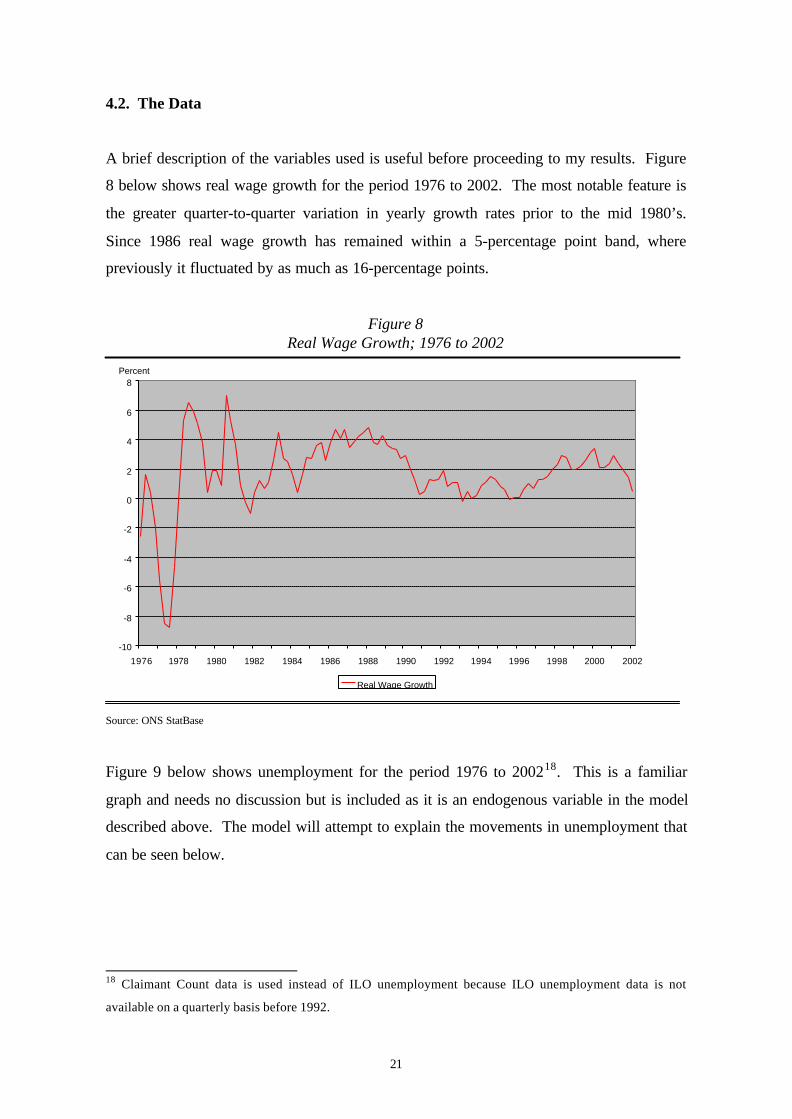
A brief description of the variables used is useful before proceeding to my results. Figure

8 below shows real wage growth for the period 1976 to 2002. The most notable feature is

the greater quarter-to-quarter variation in yearly growth rates prior to the mid 1980’s.

Since 1986 real wage growth has remained within a 5-percentage point band, where

previously it fluctuated by as much as 16-percentage points.

Figure 8Real Wage Growth; 1976 to 2002

Source: ONS StatBase

Figure 9 below shows unemployment for the period 1976 to 200218. This is a familiar

graph and needs no discussion but is included as it is an endogenous variable in the model

described above. The model will attempt to explain the movements in unemployment that

can be seen below.

18 Claimant Count data is used instead of ILO unemployment because ILO unemployment data is not

available on a quarterly basis before 1992.

-10

-8

-6

-4

-2

0

2

4

6

8

1976 1978 1980 1982 1984 1986 1988 1990 1992 1994 1996 1998 2000 2002

Percent

Real Wage Growth

22

Figure 9Unemployment; UK; 1976 to 2002

Source: ONS StatBase

Figure 10 below shows the CBI skill shortages series over the period 1976 to 2002. This

series is the same as that shown above in Figure 5 but without the other factors that limit

output and is also seasonally adjusted19. The graph shows that over the period the level of

skill shortages has fluctuated a lot, with a range of 25-percentage points20. There are also

two obvious peaks in the skill shortages series around 1979 and 1990 (and perhaps one in

2001) and the series shows some cyclical tendencies. The DfES argue that the cyclicallity

of skill deficiencies is not simply a consequence of the business cycle but also influence it.

Blake et al [5] conclude that, “Skill shortages do not simply reflect recruitment difficulties

associated with the stage of the cycle” and so, the variations in skill shortages could have

important implications for real wage growth and unemployment and are not simply a

cyclical phenomenon. The focus of this paper therefore, is to assess what affect

movements in the level of skill shortages have on unemployment and real wage growth.

19 The CBI data was seasonally adjusted to correspond with all the other series to be used in my regression

analysis, all the other series are seasonally adjusted.20 See tables 2 and 3 for descriptive statistics.

0

2

4

6

8

10

12

1976 1978 1980 1982 1984 1986 1988 1990 1992 1994 1996 1998 2000 2002

Percent

Unemployment

23

Figure 10CBI Skill Shortages; 1976 to 2002, seasonally adjusted

Source: CBI Industrial Trends Survey

Descriptive statistics for all of the variables over the sample period 1976 Q1 to 2002 Q1

are shown in table 2 below21. The table is split into endogenous and exogenous variables

to aid interpretation. From the table it can be seen that over the sample period there is

much more variation in real wage growth than in unemployment, with ranges of 15.8 and

7.5 respectively. The standard deviations are however, both around 2.5. Given that I have

estimated my model over a smaller period than my sample, I have also reported

descriptive statistics for the reduced sample of 1986 Q1 to 2002 Q1, these are shown in

table 3 below.

21 Graphs of all the variables are not included due to limited space. Plots of all the variables were however

produced and raised issues such as nonstationarity and cointegration, which will be discussed later.

0

5

10

15

20

25

30

1976 1978 1980 1982 1984 1986 1988 1990 1992 1994 1996 1998 2000 2002

Percent

Skill shortages

24

Table 2Descriptive Statistics; 1976 Q1 to 2002 Q1

Source: CBI Industrial Trends Survey; ONS StatBase

Table 3Descriptive Statistics; 1986 Q1 to 2002 Q1


In this reduced sample the range of the unemployment series is greater than that of the real

wage growth series, 7.5 and 5 respectively, and the standard deviation of unemployment is

larger at 2.33 compared to 1.39. These differences between the two samples are due to the

excess volatility of the real wage growth series prior to1986, with the estimation sample

(1986 Q1 to 2002 Q1) excluding this period.

Direct comparison of the real wage growth series and the unemployment series with the

skill shortage series give some initial idea as to the likely effect of skill shortages on real

wage growth and unemployment. Figure 11 below shows the UK unemployment rate

against the CBI skill shortages series for the period 1971 to 2002.

Variables Obs Mean Median Std. Dev. Max Min Range

Wgrowth 65 2.04 2.00 1.39 4.80 -0.20 5.00UN 65 6.79 7.00 2.33 10.60 3.10 7.50

SkillShortage 65 11.98 11.22 5.69 27.04 2.90 24.14GDPGrowth 65 0.64 0.60 0.55 2.10 -1.20 3.30

StockGDP 65 105.17 102.00 5.25 117.00 100.00 17.00GFCF 65 30.99 29.57 4.97 40.79 21.96 18.83R 65 8.11 6.73 3.21 15.14 3.87 11.27

Endogenous

Exogenous

Variables Obs Mean Median Std. Dev. Max Min Range

Wgrowth 105 1.76 1.90 2.46 7.00 -8.80 15.80UN 105 6.78 6.90 2.49 10.60 3.10 7.50

SkillShortage 105 11.79 11.22 6.36 27.04 2.04 25.00GDPGrowth 105 0.58 0.60 0.83 4.20 -2.40 6.60

StockGDP 65 105.17 102.00 5.25 117.00 100.00 17.00GFCF 105 26.82 27.12 6.66 40.79 17.63 23.16R 105 9.34 9.38 3.46 16.97 3.87 13.10

Endogenous

Exogenous

25

Figure 11CBI Skill Shortages and Unemployment; 1971 to 2002, seasonally adjusted


The graph above shows that there is a strong inverse relationship between skill shortages

and the unemployment rate, especially after 1980. This relationship is disrupted slightly

around 1998 when skill shortages decreased and so did unemployment. The DfES argue

that “skills deficiencies are simply not a cyclical phenomenon”22 but actually influence the

business cycle. The graph above suggests that we would expect skill shortages to have a

negative effect on unemployment.

A large proportion of firms in the Employer Skill Surveys highlighted increased salaries as

a solution to skill shortages23. This indicates that a possible response to skill shortages

and/or recruitment difficulties could be increased salaries and hence increased real wage

growth. We might therefore expect real wage growth to increase during periods of

22 See Bosworth et al [7].23 Increase salaries was the most common solution to skill shortages adopted with about 50% of respondents,

in both the ESS 1999 and ESS 2001, adopting increased salaries as a solution to skill shortages.

0

10

20

30

40

50

60

1971 1973 1975 1977 1979 1981 1983 1985 1987 1989 1991 1993 1995 1997 1999 2001

CBI Survey percentage

0

2

4

6

8

10

12Unemployment rate

CBI skill shortages Unemployment rate

26

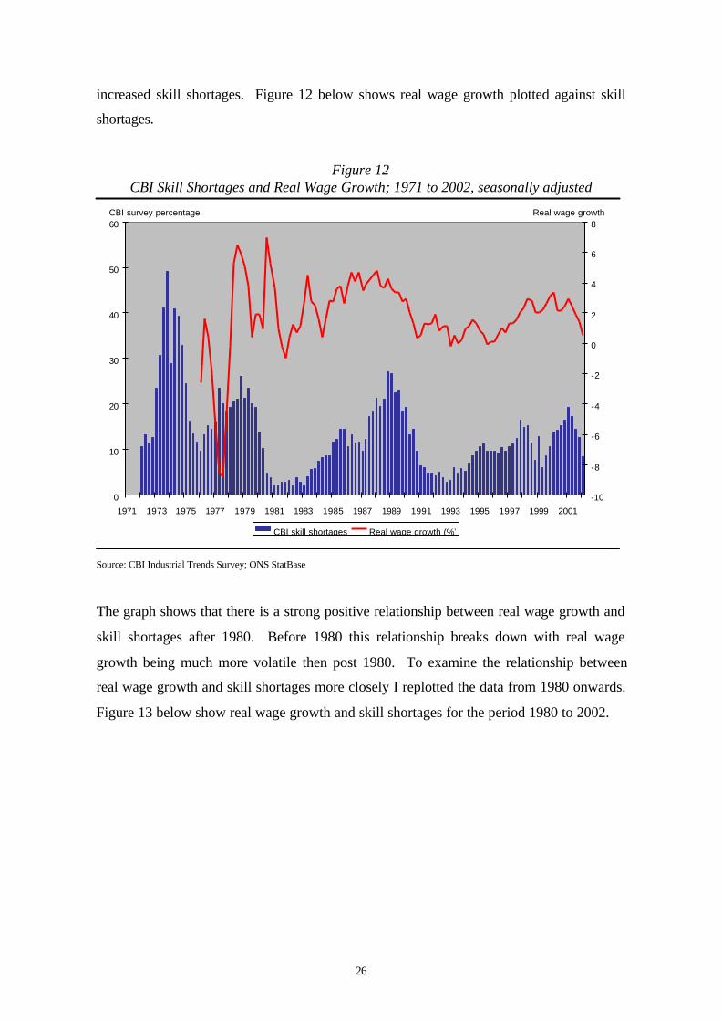
increased skill shortages. Figure 12 below shows real wage growth plotted against skill

shortages.

Figure 12CBI Skill Shortages and Real Wage Growth; 1971 to 2002, seasonally adjusted


The graph shows that there is a strong positive relationship between real wage growth and

skill shortages after 1980. Before 1980 this relationship breaks down with real wage

growth being much more volatile then post 1980. To examine the relationship between

real wage growth and skill shortages more closely I replotted the data from 1980 onwards.

Figure 13 below show real wage growth and skill shortages for the period 1980 to 2002.

0

10

20

30

40

50

60

1971 1973 1975 1977 1979 1981 1983 1985 1987 1989 1991 1993 1995 1997 1999 2001

CBI survey percentage

-10

-8

-6

-4

-2

0

2

4

6

8Real wage growth

CBI skill shortages Real wage growth (%)

27

Figure 13CBI Skill Shortages and Real Wage Growth; 1980 to 2002; seasonally adjusted


The graph shows a strong positive relationship between skill shortages and real wage

growth, especially after 1984/85. The data thus appears to support the idea that increased

skill shortages will lead to an increase in real wage growth.

5. Estimation and Sample Period

Both of the equations in the above system are overidentified24 and so were estimated by a

two-stage least squares (2SLS) procedure. Given that the equations are overidentified

2SLS gives consistent estimates of the equation coefficients. Before this was done a

version of the Hausman Specification Error Test was conducted to test for simultaneity

between unemployment and real wage growth. This test showed that simultaneity exists

between unemployment and real wage growth, and so a system of simultaneous equations

is needed to estimate a model. The presence of simultaneity also ensures that 2SLS will

24 See chapter 19 of Gurarati, D. N. Basic Econometrics. Third Edition.

0

5

10

15

20

25

30

35

40

45

50

1980 1982 1984 1986 1988 1990 1992 1994 1996 1998 2000 2002

CBI survey percentage

-4

-2

0

2

4

6

8Real wage growth

CBI skill shortages Real wage growth %

28

give estimators that are consistent and efficient. Without such simultaneity 2SLS will

yield estimators that are consistent but not efficient.

My sample period is from 1976 Q1 to 2002 Q1, although my equations are estimated over

the period 1986Q1 to 2002 Q1, due to the inclusion of the stock/GDP variable in the wage

equation, for which, data is not available for the entire sample period25. The rest of the

sample period can however, be used to produce a backward forecast for unemployment to

see how well the model predicts past variations.

6. Basic Results

6.1. 2SLS Estimates

The equations for the period 1986 Q1 to 2002 Q1 were estimated by 2SLS as follows,

111

41

214.0297.0643.0/216.0080.0

093.0295.0587.0175.077.29

−−−

−−

++++−

+−++−=

ttttt

ttttt

GFCFGDPGrowthGDPGrowthGDPStockageSkillShort


441 0255.0133.0205.0180.1034.00646.0 −−− +−−+−= tttttt rGDPGrowthUNUNWGrowthUN

6.2. Real Wage Growth Equation

Table 4 below shows a summary of the results for the 2SLS estimation of the real wage

growth equation.

25 This gives a sample of 65 observations, which is generally considered enough for a 2SLS estimation

procedure. The presence of a possible structural break in the real wage growth equation also justifies

limiting the original sample of 105 observations. This is discussed later.

29

Table 4Summary of Real Wage Growth Equation; 1986 to 2002; 2SLS

Table 4 above shows that all the variables are statistically significant at the 1% level,

except for one quarter lagged GDP growth, which is significant at 5%, and

unemployment, which is significant at the 10% level, with a p-value of 8.7%26. The

variables explain a large proportion of the variation in real wage growth, with an adjusted

R squared of 0.932. This is quite high considering the volatility of real wage growth over

the sample period. The regression is highly statistically significant, with the hypothesis

that all coefficients are jointly zero rejected at all significance levels.

The skill shortage variable was statistically significant in nearly all of the alternate

specifications that I tried and always had a positive coefficient. Lagged skill shortages

was also significant in various specifications and always had a negative coefficient. The

coefficient on lagged skill shortages was always less in absolute value than the coefficient

26 It should be noted here that the reported standard errors are not those from the second stage regression of

the 2SLS procedure but are corrected standard errors.

Variable Coefficient s.e t-value Sig

Constant -29.765 5.330 -5.585 0.0000UN 0.175 0.100 1.745 0.0866

WGrowth_1 0.587 0.080 7.306 0.0000WGrowth_2 -0.295 0.084 -3.513 0.0009

SkillShortage 0.093 0.023 4.070 0.0002SkillShortage_1 -0.080 0.023 -3.530 0.0008Stock/GDP 0.216 0.034 6.328 0.0000

GDPGrowth 0.643 0.121 5.337 0.0000GDPGrowth_1 0.297 0.141 2.112 0.0392GFCF 0.214 0.056 3.847 0.0003

Multiple R R SquareAdjusted R

Square s.e

Equation 1 0.965 0.932 0.921 0.390

DFSum ofSquares

MeanSquare F

Regression 9 114.491 12.721 83.440Residual 55 8.385 0.152

30

on skill shortages. This indicates that the initial effect of an increase in skill shortages is

reversed slightly in the next quarter. Other lags of the skill shortages variable were never

significant.

GDP growth had the expected sign in the real wage growth equation but the

unemployment coefficient was always negative, this is the opposite of what would be

expected. The reason for the unemployment variable having a negative coefficient is

mostly likely to do with the fact that we are using real wage growth. High levels of

unemployment tend to be accompanied by low price level growth and so, given that

nominal wages are fixed for some workers high unemployment can result in real wage

growth27.

Note the significance of the variable Stock/GDP in the above equation. The statistical

significance of this variable in the specifications I tried justified reducing the estimation

sample in order to include it. Without this variable the wage growth equation was less

robust and had much less explanatory power. Although there is some economic

justification for the Stock/GDP variable being important its significance in the equation is

surprising.

I also tested a linear wage equation for structural break in the early 1980’s, before which

real wage growth can be seen to be much more volatile. I could not reject that there was a

structural break between 1980 and 1982 and so felt justified in reducing my estimation

sample to start in 1986 Q1. A wage equation over my full sample had considerably less

explanatory power and was less robust.

Figure 14 below shows the predicted values obtained from the model against actual real

wage growth.

27 This problem emerges from the fact that a complete structural model should consist of a wage, a price, and

an unemployment equation.

31

Figure 14Real Wage Growth and Modelled Real Wage Growth; 1986 to 2002

The graph above shows that the model performs well considering the volatility of real

wage growth. Real wage growth tends to be difficult to model given that it consists of two

endogenous variables that are related to each other (nominal wage growth and inflation).

The graph above shows that the model performs well and predicts real wage growth very

close to actual real wage growth. This can be seen further in Figure 15 below.

-1

0

1

2

3

4

5

6

1986 1988 1990 1992 1994 1996 1998 2000 2002

Per cent

Actual real wage growth Modelled real wage growth

32

Figure 15 Residuals: Real Wage Growth Equation

Figure 15 above shows a scatter plot of the residuals for the real wage growth equation.

The scatter plot shows that by visual observation the residuals exhibit no autocorrelation

and that there are not any obvious outliers. The residuals also fall within a 1-point band

either side of zero.

6.3. Unemployment Equation

Table 5 below shows a summary of the results for the unemployment equation. The table

show that real wage growth is statistically significant at the 5% level, whilst all other

variables, except for the constant, which has a p-value of 0.36, are statistically significant

at the 1% level. The model has very high explanatory power with an adjusted R squared

of 0.996. It also has a very high F-value of some 3558.760, which means that the

regression is highly statistically significant, with the hypothesis that all coefficients are

jointly zero rejected at all significance levels. . The residual sum of squares is much lower

than that for the wage equation at 1.144. This is as expected given that unemployment is a

much less volatile series than real wage growth.

-1

-0.8

-0.6

-0.4

-0.2

0

0.2

0.4

0.6

0.8

1

0 10 20 30 40 50 60 70

Observation (ordered by time)

Value

33

Table 5Summary of Unemployment Equation; 1986 to 2002; 2SLS

The skill shortage variable was never statistically significant in any of the alternate

specifications that I tried, but did always have a negative sign as was expected. This

corresponds with DfES research that concludes that, although there is a negative

relationship between skill shortages and unemployment “in statistical terms, this

relationship is relatively weak”28. The system of equations above ensures that changes in

skill shortages do affect unemployment but this is through their effect on real wage

growth. The exclusion of skill shortages from the unemployment equation is therefore

supported by both statistical and economic arguments.

The inclusion of the interest rate variable is not generally supported by economic theory as

entering into unemployment equations, but as other authors have found, this variable was

statistically significant in all model specifications. For this reason it has remained, even

though it has no strong theoretical foundation. The sign of the coefficient is as would be

expected.

28 See [13].


Constant 0.065 0.070097 0.922 0.3604WGrowth -0.034 0.017 -2.051 0.0448

U_1 1.180 0.027 44.415 0.0000U_4 -0.205 0.027 -7.618 0.0000

GDPGrowth -0.133 0.042 -3.169 0.0024r_4 0.026 0.007 3.585 0.0007


Square s.e

Equation 2 0.998 0.997 0.996 0.139

DFSum of Squares

Mean Square F


34

The unemployment equation was estimated over the period 1986 Q1 to 2002 Q1 but

predicted values can be produced for the whole sample period 1976Q1 to 2002 Q1, as the

unemployment equation does not include the Stock/GDP variable. The two graphs below

in figures 16 and 17 show that the model has better predicted power over 1986 to 2002

than over the entire period. This could be due to the structural break discussed earlier but

is most likely due to the model being estimated over the later period.

Figure 16Unemployment Rate and Modelled Unemployment Rate; 1986 to 2002

In Figure 17 below the pre 1986 predicted values are essentially a backward forecast,

made using the recorded values of the variables in the unemployment equation to predict

the level of unemployment. This can then be compared to the actual level. This backward

forecast performs very well over this large period picking up the main trend in the

unemployment rate. The inclusion of lagged unemployment in the unemployment

equation does however mean that the ability to produce a backwards forecast should not

be overstated, as the lagged value of unemployment will be doing a lot of the work when

producing this forecast.

0

2

4

6

8

10

12

1986 1988 1990 1992 1994 1996 1998 2000 2002

Per cent

Actual unemployment rate Modelled unemployment rate

35

Figure 17Unemployment Rate and Modelled/Forecast Unemployment Rate; 1977 to 2002

Figure 18 below shows a scatter plot of the residuals for the unemployment equation and

shows that the residuals for the estimated equation show no obvious autocorrelation or

outliers. The graph also shows that the unemployment equation performs better than the

real wage growth equations with the residuals within a 0.4-point band either side of zero.

The better performance of the unemployment equation is also outlined by the residual sum

of squares for the equations. The residual sum of squares for the unemployment equation

is only 1.144 compared to a residual sum of squares for the real wage growth equation of

8.385. This is not surprising given the variation of real wage growth.

0

2

4

6

8

10

12

1977 1979 1981 1983 1985 1987 1989 1991 1993 1995 1997 1999 2001

Per cent

Actual unemployment rate Modelled unemployment rate

36

Figure 18Residuals: Unemployment Equation; 1986 to 2002

A scatter plot of the residuals over the full sample period, including the backwards

forecast shows, as does figure 17 above, that the model performs better over the

estimation period than over the forecast period.

7. Model Evaluation and Diagnostics

One of the problems that emerge when looking at time series data is the implication of

nonstationarity and cointegration. Casual observation of the unemployment series, in

figure 9 above, suggests that the series may be nonstationary. To test the unemployment

time series for nonstationarity an autocorrelation function (ACF) was produced, this is

shown below in figure 19.

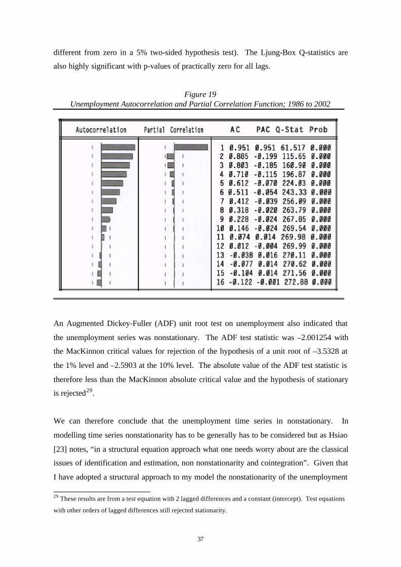
Figure 19 shows the correlogram for up to 16 lags (4 years). The main feature of the

correlogram is that it starts of at a very high value of 0.951 and tapers of gradually over

further lags. At lag 8 (2 years) the autocorrelation coefficient is still 0.318, implying that

there is some correlation between unemployment levels two years apart. The correlogram

is therefore indicative that the time series is nonstationary. Figure 8 above also shows that

all the coefficients up to lag 8 are individually statistically significance (statistically

-0.4

-0.3

-0.2

-0.1

0

0.1

0.2

0.3

0.4

0 10 20 30 40 50 60 70

Observation (ordered by time)

Value

37

different from zero in a 5% two-sided hypothesis test). The Ljung-Box Q-statistics are

also highly significant with p-values of practically zero for all lags.

Figure 19Unemployment Autocorrelation and Partial Correlation Function; 1986 to 2002

An Augmented Dickey-Fuller (ADF) unit root test on unemployment also indicated that

the unemployment series was nonstationary. The ADF test statistic was –2.001254 with

the MacKinnon critical values for rejection of the hypothesis of a unit root of –3.5328 at

the 1% level and –2.5903 at the 10% level. The absolute value of the ADF test statistic is

therefore less than the MacKinnon absolute critical value and the hypothesis of stationary

is rejected29.

We can therefore conclude that the unemployment time series in nonstationary. In

modelling time series nonstationarity has to be generally has to be considered but as Hsiao

[23] notes, “in a structural equation approach what one needs worry about are the classical

issues of identification and estimation, non nonstationarity and cointegration”. Given that

I have adopted a structural approach to my model the nonstationarity of the unemployment

29 These results are from a test equation with 2 lagged differences and a constant (intercept). Test equations

with other orders of lagged differences still rejected stationarity.

38

series is not an issue 30, all that needs to be considered are the issues of identification and

simultaneity bias31.

Table 6 below shows the diagnostic results for the estimated system above. The first 8

lines show the diagnostic test for the separate equations, whilst the following three lines

show the tests for the whole system. The single equation tests consist of an error

autocorrelation test, a normality test, a heteroscedasticity test, and an autoregressive

conditional heteroscedasticity test (ARCH). The system tests are then vector tests of the

same type, excluding the ARCH test. A Vector Portmanteau test was also reported but is

only a valid test in a VAR (Vector Autoregression).

Table 6Diagnostic Results for 2SLS Estimation

U :AR 1- 2 F( 2, 51) = 19.812 [0.0000] **Wgrowth :AR 1- 2 F( 2, 51) = 1.0557 [0.3554]U :Normality Chi^2(2)= 0.026099 [0.9870]Wgrowth :Normality Chi^2(2)= 1.4692 [0.4797]U :ARCH 1 F( 1, 51) = 2.5196 [0.1186]Wgrowth :ARCH 1 F( 1, 51) = 0.17257 [0.6796]U :Xi^2 F(22, 30) = 1.4446 [0.1725]Wgrowth :Xi^2 F(22, 30) = 0.60327 [0.8884]

Vector AR 1-2 F( 8,104) = 2.9736 [0.0049] **Vector normality Chi^2( 4) = 1.9347 [0.7478]Vector Xi^2 F(66, 96) = 1.0376 [0.4297]

As can be seen above the model performs well in all but the error autocorrelation test for

the unemployment equation and the vector autocorrelation test. The nonstationarity of the

unemployment series could be causing the model to fail this diagnostic test, even so, it is

possible to handle the complication of the error term being autocorrelated by using an

alternative estimation technique to 2SLS. Using Zellner’s seemingly unrelated regressions

(SURE) estimation technique to estimate the coefficients in my system of equations the

problem of autocorrelated errors can be resolved.

30 I also estimated an equation similar to my model with the second difference of unemployment, which is

stationary, as an endogenous variable instead of unemployment, the results were very similar.31 See section 5.

39

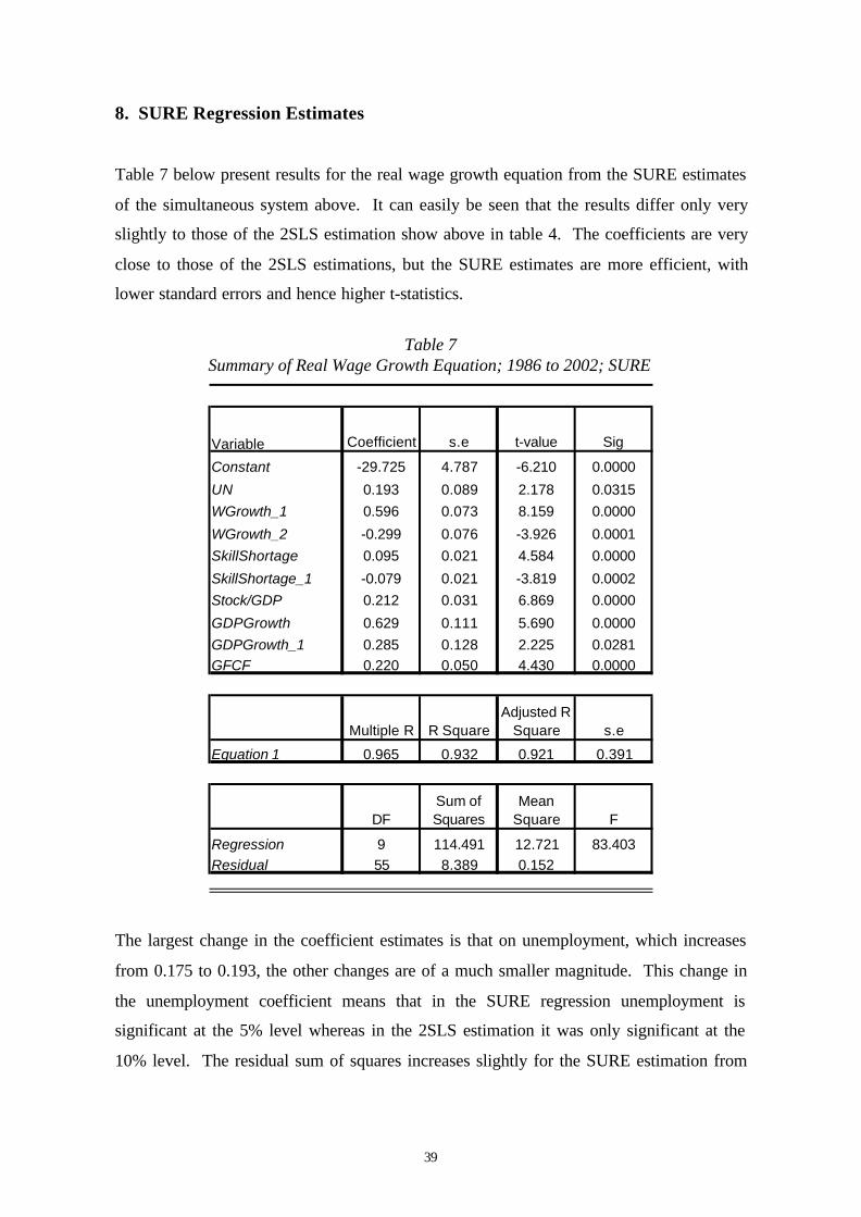
8. SURE Regression Estimates

Table 7 below present results for the real wage growth equation from the SURE estimates

of the simultaneous system above. It can easily be seen that the results differ only very

slightly to those of the 2SLS estimation show above in table 4. The coefficients are very

close to those of the 2SLS estimations, but the SURE estimates are more efficient, with

lower standard errors and hence higher t-statistics.

Table 7Summary of Real Wage Growth Equation; 1986 to 2002; SURE

The largest change in the coefficient estimates is that on unemployment, which increases

from 0.175 to 0.193, the other changes are of a much smaller magnitude. This change in

the unemployment coefficient means that in the SURE regression unemployment is

significant at the 5% level whereas in the 2SLS estimation it was only significant at the

10% level. The residual sum of squares increases slightly for the SURE estimation from


Constant -29.725 4.787 -6.210 0.0000

UN 0.193 0.089 2.178 0.0315WGrowth_1 0.596 0.073 8.159 0.0000

WGrowth_2 -0.299 0.076 -3.926 0.0001SkillShortage 0.095 0.021 4.584 0.0000

SkillShortage_1 -0.079 0.021 -3.819 0.0002Stock/GDP 0.212 0.031 6.869 0.0000

GDPGrowth 0.629 0.111 5.690 0.0000GDPGrowth_1 0.285 0.128 2.225 0.0281GFCF 0.220 0.050 4.430 0.0000


Square s.e

Equation 1 0.965 0.932 0.921 0.391

DFSum of Squares

Mean Square F


40

8.385 to 8.389 but this has no real effect on the explanatory power of the regression,

measure by its R-squared or F-statistic.

Table 8 below reports the results of the SURE estimation of the unemployment equation.

As with the real wage growth equations the SURE estimates are very close to the 2SLS

estimates and again the SURE estimation is more efficient with lower standard error. All

the t-values are higher except for the real wage growth variable, which falls slightly, as the

coefficient falls in absolute value. The p-value of the wage growth variable increases

from 0.0448 in the 2SLS estimation to 0.0510 in the SURE estimation.

Table 8Summary of Unemployment Equation; 1986 to 2002; SURE

The residual sum of squares of the SURE regression is slightly less than that of the 2SLS

regression at 1.139 compared with 1.144 but this is relatively unimportant considering the

very high R-squared and F-statistic of both estimates.

It should be noted here that although changes in the coefficient estimates are small, these

changes do have implications later when estimating the impact and long-run multiplier of

the system.


Constant 0.065 0.066481 0.980 0.3292

WGrowth -0.029 0.015 -1.973 0.0510U_1 1.183 0.025 47.516 0.0000

U_4 -0.206 0.025 -8.162 0.0000GDPGrowth -0.139 0.039 -3.530 0.0006r_4 0.024 0.007 3.597 0.0005


Square s.e

Equation 2 0.998 0.997 0.996 0.139

DFSum of Squares

Mean Square F


41

9. Implications of equations

9.1. Impact and Long Run Responses

In order to determine the effect of skill shortages on real wage growth and unemployment

we first have to calculate the reduced-form equations of the system above. These reduced-

form equations express unemployment and real wage growth (the endogenous variables)

solely as a function of the exogenous (predetermined) variables and the stochastic

disturbance terms. With these reduced-form equations we can calculate reduced-form

coefficients, which will be non-linear combinations of the structural coefficients estimated

above.

The reduced-form of the system of equations above is the following32,

tttttt

ttttttt

vGFCFGDPGrowthGDPStockageSkillShortageSkillShort

WGrowthWGrowthrGDPGrowthUNUNWGrowth

++++++

++++++=

−−−

−−−−−

1111109187

461544342110

/ πππππ

πππππππ

and

ttttttt

tttttt

wrUNUNGFCFGDPGrowthGDPGrowth

GDPStockageSkillShortageSkillShortWGrowthWGrowthUN

+++++++

+++++=

−−−−−

−−−

4114101918176

514342110 /

λλλλλλ

λλλλλλ

The reduced-form coefficients above are the impact, or short-run multipliers of the

system. The reduced-form coefficients, such as 11 ,λπ , give the immediate impact on real

wage growth or unemployment (the endogenous variables) of a change in a given

exogenous variable.

The reduced-form above also shows that the structural model estimated above is

overidentified. There are 16 structural coefficients, but there are 24 reduced-form

coefficients, and so 24 equations with which to estimate them. Due to this, a unique

estimation of the parameters in the model cannot be obtained by OLS; hence we have to

use 2SLS to estimate the structural coefficients. 2SLS will provide us with one estimate

per parameter.

32 See appendix for detail.

42

We can now calculate the impact response on real wage growth and unemployment of a

one-unit increase in the skill shortages variable using the 2SLS estimates of the

coefficients33.

For real wage growth the impact response is,

09245.0)034.0175.0(1

093.01 11

47 =

−×−=

−=

βαα

π

For unemployment the impact response is,

00314.0)034.0175.0(1

093.0034.01 11

413 −=

−×−×−

=−

=βα

αβλ

The above impact responses imply that a one-unit (one-percentage point) increase in the

skills shortage variable leads to an immediate 0.09245-unit increase in real wage growth

(%) and a 0.00314-unit fall in the unemployment rate (%). The direction of these two

responses is as expected prior to analysis. Graphs of the skills shortage data against real

wage growth and unemployment both show relationships in the same direction as these

impact responses.

We can now also calculate the long-run response of real wage growth and unemployment

to increases in skills shortages. In long-run equilibrium34,

**/

*)(**)(*)(*)1(

119

87410321065

GFCFGDPStock

ageSkillShortrGDPGrowthUNWGrowth

ππ

ππππππππππ

++

+++++++=−−

and

***)(

*/*)(*)(*)1(

11876

543210109

rGFCFGDPGrowth

GDPStockageSkillShortWGrowthUN

λλλλ

λλλλλλλλ

++++

+++++=−−

Therefore

*1

*/1

*1

*1

*1

*11

*

65

11

65

9

65

87

65

4

65

103

65

21

65

0

GFCFGDPStockageSkillShort

rGDPGrowthUNWGrowth

−−+

−−+

−−+

+

−−

+

−−

++

−−

++

−−=

πππ

πππ

ππππ

πππ

ππππ

ππππ

πππ

33 Responses for the SURE estimation will be reported and discussed later.34 See appendix.

43

and

*1

*1

*1

*/1

*1

*11

*

109

11

109

8

109

76

109

5

109

43

109

21

109

0

rGFCFGDPGrowth

GDPStocktageSkillsShorWGrowthUN

−−

+

−−

+

−−

++

−−

+

−−

++

−−

++

−−=

λλλ

λλλ

λλλλ

λλλ

λλλλ

λλλλ

λλλ

The long-run coefficients on skills shortages for real wage growth and unemployment are

thus the following respectively,

01820.02933.05835.01

07953.009245.01 65

87 =+−

−=

−−+

ππππ

01429.02038.01730.1100270.000314.0

1 109

43 −=+−+−

=−−

+λλ

λλ

These long-run coefficients imply that following a one-percentage point increase in skills

shortages the overall long-run effect on real wage growth is a 0.0182-percentage point

increase and on unemployment a 0.01429-percentage point decrease.

9.2. Comparison of 2SLS and SURE Estimates

As noted above the differences in the estimated coefficients of the 2SLS and SURE

estimates are minimal, the differences in the impact and long-run responses are greater and

are of more importance when quantifying the effect of skill shortages on real wage growth

and unemployment. Table 9 below shows a comparison of the impact and long-run

responses to a one-percentage point increase in skill shortages for the estimated 2SLS and

SURE equations.

44

Table 10Comparison of 2SLS and SURE Responses to a one-percentage point Increase in Skill

Shortages

The table above shows that the impact and long-run responses of real wage growth to a

one-percentage increase in skill shortages differ very little between the 2SLS and SURE

estimates. Both the SURE and 2SLS estimates show an impact response that is greater

than the long-run response, with the effect on increased real wage growth on

unemployment reducing the effect of an increase in skill shortages in the long-run. The

SURE estimation implies a slightly larger response than the 2SLS estimation. The SURE

estimation produces a greater impact response of 0.09447 compared to 0.09245 and a

greater long-run response of 0.02258 compared to 0.01820. This implies that the 2SLS

estimation procedure may underestimate the impact of skill shortages on real wage

growth.

The SURE estimation of the unemployment equation implies a greater increase in

unemployment between the impact and long-run. The SURE impact response is less than

that of the 2SLS estimation in absolute terms, at –0.00274 compared to –0.00314, but the

long-run response is greater in absolute terms, at –0.01624 compared to –0.01429. Both

the 2SLS and SURE estimates imply that after an initial small impact response the effect

on unemployment in the long-run increases. For the 2SLS estimation the long-run

response is about four and a half times the impact response, whereas for the SURE

estimation the long-run response is about six times the impact response.

The SURE estimation therefore produces greater long-run responses for both real wage

growth and unemployment. In terms of impact responses the real wage growth impact

response is greater but the impact response of unemployment is smaller in absolute terms.

Both estimation techniques do however produce the same type of effect on unemployment

Response Variable 2SLS SURE

Wgrowth 0.09245 0.09447UN -0.00314 -0.00274

Wgrowth 0.01820 0.02258UN -0.01429 -0.01624

Impact

Static Long-run

45

and real wage growth. A one-percentage point increase in skill shortages causes an

overshooting of real wage growth with a large impact response, this response falls by

about factor four over the long-run. In terms of unemployment we have a small initial

response but a much more significant long-run response.

9.3. Sensitivity Analysis

Table 11 below shows how the impact and long run responses vary when one standard

error is added or subtracted from the coefficient estimates. The results are presented for

both the 2SLS estimates and the SURE estimates.

Table 11Sensitivity Analysis of Response to one-percentage point increase in skill shortages; 2SLS

and SURE Estimates.

Table 11 above shows that the impact responses are quite robust always giving the same

sign in table 10. The long-run responses are however less robust, although the results are

slightly misleading. The long-run responses tend to have the opposite sign to those in

table 10, the problem here however, is that we are adding a standard error to each

coefficient whilst there is a negative coefficient on real wage growth in the unemployment

equation. Such an analysis is complicated by the complexities of computing the long run

responses, which are made up of a large number of different estimated coefficients. The

robustness of the impact responses is a better indicator of performance35, with the

calculated direction of the effect of skill shortages the same as when using the original

coefficient estimates.

Response Variable 2SLS SURE 2SLS SURE

Wgrowth 0.06994 0.07406 0.11546 0.11554UN -0.00354 -0.00328 -0.00196 -0.00162

Wgrowth -0.03700 -0.02917 0.10774 0.10230UN 0.01998 0.01414 0.04145 0.03537

Impact

Static Long-run

coefficients minus 1 standard error

coefficients plus 1 standard error

46

9.4. Implications

If we use the SURE estimates of the coefficients for the system of equations we have

long-run responses to a one-percentage point increase in skill shortages of 0.023-

percentage points for real wage growth and –0.016-percentage points for unemployment.

These responses are quite small but they are not insignificant, in order to assess the full

effects of skill shortages their variability and level of fluctuation over time is important.

Figure 10 and table 3 above showed that skill shortages over the period 1986 to 2002

fluctuated quite dramatically with a range of some 24-percentage points. Sharp

fluctuations in the level of skill shortages will have important implications for real wage

growth and unemployment. Table 12 below shows descriptive statistics for quarterly and

yearly changes of the skill shortages variable.

Table 12Skill Shortages, Quarterly and Yearly Changes; 1986 to 2002

Table 12 above shows that on average over periods of up to one-year skill shortages do

not matter, with means close to zero for 1 to 4 quarter changes. The two-year change in

skill shortages has a mean of 0.50, which will produces changes in real wage growth and

unemployment that are negligible. All that the means imply however is that the level of

skill shortages over the period have on average remained constant. This however misses

the importance of the fluctuations that occur in skill shortages and their effect on real

wage growth and unemployment.

In terms of the importance of skill shortages on real wage growth and unemployment the

maximum and minimum columns of table 12 above are most important. Looking at the

35 Remember here that the impact responses are the reduced-from coefficients.

Skill Shortages Mean Median Std. Dev. Max Min Range

one-quarter change -0.09 0.30 2.60 6.00 -6.66 12.66

two-quarter change -0.12 0.03 3.49 7.66 -7.95 15.61

three-quarter change -0.09 0.32 4.50 9.07 -9.69 18.75

one-year change 0.00 0.96 5.31 11.72 -12.78 24.50two-year change 0.50 1.93 7.66 17.05 -20.24 37.29

47

one-year change the maximum increase in skill shortages is some 11.72-percentage points,

which occurs between 1987 Q1 and 1988 Q1. Such a movement in skill shortages will

lead to, using my SURE estimates, a 0.26-percentage points increase in real wage growth

and a 0.2-percentage points fall in unemployment. For the two-year change of skill

shortages we see a maximum increase of 17.05, which leads to a 0.4-percentage point

increase in real wage growth and a 0.28-percentage point fall in unemployment.

Movements in real wage growth and unemployment of this magnitude are significant and

even the maximum one-quarter change produces long run movements in real wage growth

and unemployment of 0.14 and –0.1 percentage points respectively.

The minimum changes in the table above can be interpreted the same way and give falls in

skill shortages as opposed to increases. These also show significant falls in skill

shortages, which have significant effects on real wage growth and unemployment. It is

clear that the basic responses given in sections 9.1. and 9.2. do not give the full picture of

the importance of skill shortages. The large fluctuations in skill shortages over time have

important implications for real wage growth and unemployment, producing significant

movements in these variables.

10. Skill shortages and unemployment

The skill shortage variable is only present in the real wage growth equation, looking at

figure 11 above this might seem unreasonable, as the unemployment rate seems to have a

strong inverse relationship with the skills shortage series. The skill shortage variable was

however never significant at even the 10% level in any of the alternate specifications tried.

One important point to note here is that, although the skill shortages variable does not

enter the unemployment equation, the set up of the model means that skill shortages do

affect unemployment. The impact and long-run multipliers calculated above show that the

affect of skill shortages on unemployment works in the same direction as the graph in

figure 11 above predicts. Skill shortages do not affect unemployment directly they do

affect unemployment through their affect on real wage growth. This affect is in the

direction that was expected prior to regression analysis. The following discusses why skill

48

shortages might not have been statistically significant in the unemployment equation even

thought its effect on unemployment is captured in the model.

The CBI skill shortages data has limitations, in that firms could be more likely to

recognise skill shortages when unemployment is low and labour is scarcer. During

periods of high unemployment other factors, such as lack of orders or sales, are likely to

be more noticeable in limiting output. This idea can be seen in figure 5 above where it can

be seen that the majority of firms in the survey see orders as the main factor limiting sales.

It is only in periods of very low unemployment (early 1970’s and early 1990’s) when the

importance of a lack of skilled labour grows. The negative relationship shown in figure

11 above could therefore be simply due to the way the survey is conducted. In buoyant

periods with high growth and strong and growing demand the main factor that limits

output, lack of sales or orders, becomes less important and hence firms find that lack of

skilled labour becomes an increasingly important factor. In this case the actual level of

skill shortages may not actually have increased. As noted above in section 2.1, DfES

research suggests that a firm’s recognition of skill shortages and internal skill gaps is

related to their performance. This supports the idea that skill shortages are more likely to

be reported during periods of low unemployment.

The model above predicts that skill shortages affect unemployment thorough real wage

growth and not directly. There is evidence that the model is picking up the true

relationship between skill shortages and unemployment. If we look at skill shortages at a

regional level in the years of the two Employer Skills Surveys (ESS) (1999 and 2001) we

can see that at this level skills shortages show much more correlation with earnings than

with unemployment.

Figures 20 and 21 below shows regional skill shortages plotted against regional

unemployment and regional earnings growth for the ESS 1999 (note the inverted

unemployment axis).

49

Figure 20Regional Claimant Count and Skill Shortages; ESS 1999

Source: ESS 1999 (IER/IFF)

Figure 21Regional Earnings and Skill Shortages; ESS 1999

Source: ESS 1999 (IER/IFF)

0

5

10

15

20

25

Yorkshire&Humber

EastMidlands

South West WestMidlands

North East East London South East All NorthWest

Percentage of respondents

0.5

1.5

2.5

3.5

4.5

5.5

6.5

7.5

Claimant Count %

Skills shortage vacancies Claimant count

0

5

10

15

20

25

Yorkshire&Humber

EastMidlands

South West WestMidlands

North East East London South East All NorthWest

Percentage of respondents

300.00

350.00

400.00

450.00

500.00

550.00

600.00

Earnings

Skills Shortage vacancies Earnings

50

Regional unemployment does show some correlation with regional skill shortages but this

correlation is not as strong as that between regional earnings and skill shortages. This

suggests that the model may have picked up the true relationship between earnings,

unemployment and skill shortages. The differences in unemployment and earnings across

regions is obviously due to a number of factors but the graphs do provide some support for

the exclusion of skill shortages from the unemployment equation and support the

conclusion that skill shortages affect unemployment thorough wage growth and not

directly.

This conclusion is also supported by DfES research, which concludes that, “There is a

negative relationship between the incidence of skill shortage vacancies and the local

unemployment rate (i.e. in general, low unemployment rate areas tend to have a higher

than average incidence of skill shortage vacancies, and vice versa). However, in statistical

terms, this relationship is relatively weak”36. This conclusion emerges, as there are areas

where high levels of skill shortages co-exist with high levels of unemployment.

The insignificance of skill shortages in the unemployment equation could therefore be due

simply due to data considerations and the type of data being used as a proxy to measure

skill shortages. If we assume the data gives an accurate measure of skill shortages,

regional data seems to support the model that has been developed above, supporting the

conclusion that skill shortages affect real wage growth, which in turn affects

unemployment. Hence the inclusion of the skill shortage variable in the real wage

equation but not in the unemployment equation is justified.

11. Future research

An alternate modelling technique that was investigated was the use of a vector

autoregression (VAR) instead of a simultaneous structural equation approach. The

advantage of this approach is that it is not based on a priori assumptions about the

determinants of real wage growth, unemployment or skill shortages. A VAR approach

was tried but with little success. I believe this failure to be due to the weak statistical link

between skill shortages and unemployment and also the nonstationarity of unemployment.

36 See [13].

51

This is in accordance with work by Bosworth et al [7] who find no statistically significant

link between the unemployment rate and the incidence of skill shortage vacancies. A

vector error correction (VEC) model would be more appropriate given the nonstationarity

of unemployment and some of the other variables that I have used37.

The recent Employer Skill Surveys have highlighted the importance of regional

differences in skill shortages, with regions such as the South East and London with much

higher densities of skill shortages than areas such as the North East. The BCC provides a

good source of regional skill shortages data that could be used to model its effect on

regional wage growth and unemployment. The only problem with using this data is its

limited time series and its measure of skill shortages being a much broader and less well

defined than those of the Employer Skill Surveys.

One other possible area of future research would be to look at the effect of occupational

skill shortages on unemployment and wage growth for that occupation. Following the

panel data approach of Haskel and Martin [18], CBI data could be used to investigate the

effect of skill shortage variations across industries and their effects on unemployment and

wage growth.

12. Conclusions

The model estimated above suggests that increases in skill shortages lead to increased real

wage growth and reduced unemployment. The affect on unemployment does not come

directly from the increase in skill shortages but via the affect of skill shortages on real

wage growth. Due to the relationship between real wage growth and unemployment the

long run impact of an increase in skill shortages is less than the impact response in the real

wage growth equation. For unemployment the long run response is greater than the

impact response.

The 2SLS estimation of the simultaneous model above predicts that a one-percentage

point increase in the level of skill shortages will lead to an immediate 0.09245-percentage

point increase in real wage growth. In the long run the overall effect is a 0.0182-

37 Some of the variables are also cointegrated.

52

percentage point increase. In terms of unemployment, a one-percentage point increase in

the level of skill shortages will lead to an immediate fall in unemployment of 0.00314, in

the long run this impact increases to 0.01429.

SURE estimates of the simultaneous equation model are very close to that of the 2SLS

estimation but suggest that the 2SLS estimation may under predict the effect of skill

shortages on real wage growth and unemployment. The dynamics suggested by the SURE

estimation are also the same as those of the 2SLS estimation.

The model developed above gives a good idea of the magnitude and direction of the effect

that skill shortages have on real wage growth and unemployment. This effect is small for

both real wage growth and unemployment compared with a variable such as GDP growth

but is not however negligible when looking at the fluctuations in skill shortages that occur.

Looking at the one-year change of skill shortages we can see a maximum yearly change of

11.72-percentage points, the model predicts that this would produce as much as a 0.26-

percentage points increase in real wage growth and a 0.2-percentage points fall in

unemployment.

The concept of latent skill gaps could have important implications for my model. As

DfES research points out, firm will often only recognise skill shortages when output

demand is strong. As a consequence firms will tend to understate the true level of skill

shortages. If we assume that the level of latent skill gaps is consistent over time then this

has no implications for my model, simply the absolute level of skill shortages is wrong. If

however the amount of latent skill gaps has fluctuated my model could be either over or

under predicting the effect of skill shortages.

Even taking account of the possible problems with finding a suitable measure of skill

shortages and the problems associated with latent skills gaps the model developed above

shows that skill shortages can have important implications for real wage growth and

unemployment. The model provides some statistical evidence to support the economic

intuition that skill shortages increase real wage growth and reduce unemployment.

53

References38

[1] Basmann, R. L. (1957). “A Generalized Classical Method of Linear Estimation of

Coefficients in a Structural Equation”. Econometrica, Volume 25, Issue 1, 77-83.

[2] BCC Quarterly Economic Survey. Various Issues.

[3] Bean, C. R. (1994). “European Unemployment: A survey”. Journal of Economic

Literature, Volume 32, Issue 2, 573-619.

[4] Beenstock, M. and Warburton, P. (1982). “An Aggregate Model of the UK Labour

Market”. Oxford Economic Papers, Volume 34, Issue 2, 253-275.

[5] Blake, N., Dods, J. and Griffiths, S. (2000). “Employer Skill Survey: Existing

Evidence and its use in the Analysis of Skill Deficiencies”. DfES Publications

(September 2000, Ref. SKT 30).

[6] Bosworth, D. L., Davies, R., Hogarth, T., Wilson, R. A. and Shury, J. (2000).

“Employer Skills Survey 1999: Statistical Report”. DfES Publication (September 2000,

Ref. SKT 31)

[7] Bosworth, D. L., Davies, R. and Wilson, R. A. (2001). “Skills and Performance: An

Econometric Analysis of Employers Skill Survey 1999”. DfES Publication (October

2001, Ref. SME 1).

[8] Campbell, M., Baldwin, S., Johnson, S., Chapman, R., Upton, A. and Walton, F.

(2002). “Skills in England 2001”. Labour Market Trends, Volume 110, Number 1, 42-

44. http://www.statistics.gov.uk/downloads/theme_labour/LMT_January02.pdf#page=40

[9] CBI Quarterly Industrial Trends Survey. Number 165, July 2002 and various other

issues.

38 All DfES and DfEE publications can be accessed at www.skillsbase.dfes.gov.uk

54

[10] Dearden, L., McIntosh, S., Myck, M. and Vignoles, A. (2000). “The Returns to

Academic, Vocational and Basic Skills in Britain”. Skills Task Force Research Paper 20.

DfEE Publications (Ref. SKT 27, Research Ref. RR192).

[11] DfEE. (2000). “Skills for all: Proposals for a National Skills Agenda. Final Report

of the National Skills Taskforce”. DfEE Publications (Ref. SK 728).

[12] DfEE. (2000). “Skills for all: Research Report from the National Skills Task

Force”. DfEE Publications (June 2000, Ref. SKT 29).

[13] DfES. (2001). “Employers Skill Survey: Skills, Local Areas and Unemployment”.

DfES Publication (Ref. SKT 39).

[14] Frogner, M. L. (2002). “Skills Shortages”. Labour Market Trends, Volume 110,

Number 1, 17-27. http://statbase/themes/labour_market/articles/lmt_january02.asp#ss

[15] Green, F. (1999). “The Market Value of Generic Skills”. Skills Task Force

Research Paper 8. DfEE Publication (September 2000, Ref. SKT 13, Research Ref.

RR147).

[16] Gujarati, D. N. (1995). Basic Econometrics, Third Edition.

[17] Hart, P. (1990). “Skill Shortages in the United Kingdom”. National Institute of

Economic and Social Research Discussion Paper (Old Series), 169.

[18] Haskel, J. and Martin, C. (1993). “Do Skills Shortages Reduce Productivity? Theory

and Evidence from the United Kingdom.

[19] Hausman, J. A. (1978). “Specification Tests in Econometrics”. Econometrica,

Volume 46, Issue 6, 1251-1271.

[20] HM Treasury. (2002). “Developing Workforce Skills: Piloting a New Approach”.

HMSO (April 2002).

55

[21] Hogarth, T., Shury, J., Vivian, D. and Wilson, R. (2001). “Employer Skills Survey

2001: Statistical Report”. DfES Publication (September 2001, Ref. SKT 40).

[22] Hogarth, T. and Wilson, R. (2001). “Skills Matter: A Synthesis of Research on the

Extent, Causes and implications of skill deficiencies”. DfES Publication (October 2001).

[23] Hsiao, C. (1997). “Statistical Properties of the Two-Stage Least Squares Estimator

Under Cointegration”. Review of Economic Studies, Volume 64, Issue 3, 385-398.

[24] Keep, E. (1999). “Employers’ Attitude to Training”. Skills Task Force Research

Paper 15. DfEE Publication (December 1999, Ref. SKT 20, Research Ref. RR154).

[25] Layard, R. and Nickell, S. (1985). “The Causes of British Unemployment”.

National Institute Economics Review, 62-83.

[26] Lipsey, R. G. (1960). “The Relationship between Unemployment and the Rate of

Change of Money Wage Rates in the United Kingdom, 1862-1957: A Further Analysis”.

Economica, New Series, Volume 27, Issue 105, 1-31.

[27] Manning, A. (1993). “Wage Bargaining and the Phillips Curve: The Identification

and Specification of Aggregate Wage Equations”. Economic Journal, Volume 103, 98-

118.

[28] Milas, C. (1998). “Long-run Structural Estimation of Labour Market Equations

with an Application to Greece”. Economic Modelling, Volume 16, 149-161.

[29] Nakamura, A. and Nakamura, M. (1981). “On the Relationship Among Several

Specification Error Tests Presented by Durbin, Wu and Hausman”. Econometrica,

Volume 49, Issue 6, 1583-1588.

[30] Rosewell, B. (1987). “The CBI Industrial Trends Survey and Capacity Working”.

In Working Below Capacity. Macmillan

56

[31] Sims, C. A. (1980). “Macroeconomics and Reality”. Econometrica, Volume 48,

Issue 1, 1-48.

[32] Stock, J. H. and Watson, M. W. (1988). “Variable Trends in Economic Time

Series”. Journal of Economic Perspectives, Volume 2, Issue 3, 147-174.

[33] Zellner, A. (1962). “An Efficient Method of Estimating Seemingly Unrelated

Regressions and Tests for Aggregation Bias”. Journal of the American Statistical

Association, Volume 57, Issue 298, 348-368.

[34] Zellner, A. and Theil, H. (1962). “Three-Stage Least Squares: Simultaneous

Estimation of Simultaneous Equations”. Econometrica, Volume 30, Issue 1,54-78.

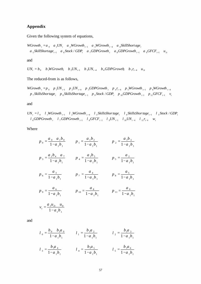
57

Appendix

Given the following system of equations,

tttttt

ttttt

uGFCFGDPGrowthGDPGrowthGDPStockageSkillShort


119187615

4431210

/ ++++++

++++=

−−−

−−

ααααα

ααααα

and

ttttttt urGDPGrowthUNUNWGrowthUN 2454431210 ++++++= −−− ββββββ

The reduced-from is as follows,

tttttt

ttttttt

vGFCFGDPGrowthGDPStocktageSkillsShortageSkillsShor

WGrowthWGrowthrGDPGrowthUNUNWGrowth

++++++

++++++=

−−−

−−−−−

1111109187

461544342110

/ πππππ

πππππππ

and

ttttttt

tttttt

wrUNUNGFCFGDPGrowthGDPGrowth

GDPStocktageSkillsShortageSkillsShorWGrowthWGrowthUN

+++++++

+++++=

−−−−−

−−−

4114101918176

514342110 /

λλλλλλ

λλλλλλ

Where

11

0100 1 βα

βααπ

−+

=11

211 1 βα

βαπ

−=

11

312 1 βα

βαπ

−=

11

7413 1 βα

αβαπ

−+

=11

514 1 βα

βαπ

−=

11

25 1 βα

απ

−=

11

36 1 βα

απ

−=

11

47 1 βα

απ

−=

11

58 1 βα

απ

−=

11

69 1 βα

απ

−=

11

810 1 βα

απ

−=

11

911 1 βα

απ

−=

11

121

1 βαα

−+

= ttt

uuv

and

11

0100 1 βα

αββλ

−+

=11

211 1 βα

αβλ

−=

11

312 1 βα

αβλ

−=

11

413 1 βα

αβλ

−=

11

514 1 βα

αβλ

−=

11

615 1 βα

αβλ

−=

58

11

4716 1 βα

βαβλ

−+

=11

817 1 βα

αβλ

−=

11

918 1 βα

αβλ

−=

11

29 1 βα

βλ

−=

11

310 1 βα

βλ

−=

11

511 1 βα

βλ

−=

11

112

1 βαβ

−+

= ttt

uuw

In long-run equilibrium the following must hold,

*41 WGrowthWGrowthWGrowthWGrowth ttt === −−

*41 UNUNUNUN ttt === −−

*1 GDPGrowthGDPGrowthGDPGrowth tt == −

*1 ageSkillShortageSkillShortageSkillShort tt == −

*// GDPStockGDPStock t =

*1 GFCFGFCFt =−

*4 rrt =−

0,0 == tt wv

Therefore

**/

*)(**)(*)(*)1(

119

87410321065

GFCFGDPStock

ageSkillShortrGDPGrowthUNWGrowth

ππ

ππππππππππ

++

+++++++=−−

and

***)(

*/*)(*)(*)1(

11876

543210109

rGFCFGDPGrowth

GDPStockageSkillShortWGrowthUN

λλλλ

λλλλλλλλ

++++

+++++=−−

Therefore in the long-run,

*1

*/1

*1

*1

*1

*11

*

65

11

65

9

65

87

65

4

65

103

65

21

65

0

GFCFGDPStockageSkillShort

rGDPGrowthUNWGrowth

−−+

−−+

−−+

+

−−

+

−−

++

−−

++

−−=

πππ

πππ

ππππ

πππ

ππππ

ππππ

πππ

59

and

*1

*1

*1

*/1

*1

*11

*

109

11

109

8

109

76

109

5

109

43

109

21

109

0

rGFCFGDPGrowth

GDPStocktageSkillsShorWGrowthUN

−−

+

−−

+

−−

++

−−

+

−−

++

−−

++

−−=

λλλ

λλλ

λλλλ

λλλ

λλλλ

λλλλ

λλλ

The Effect of Skill Shortages on Unemployment and …repec.org/res2003/Wallis.pdf1 The Effect of...

Documents

Transcript of The Effect of Skill Shortages on Unemployment and …repec.org/res2003/Wallis.pdf1 The Effect of...