The Effect of Filipino Overseas Migration on the Non ...ftp.iza.org/dp2240.pdf · The Effect of...

IZA DP No. 2240

The Effect of Filipino Overseas Migration on theNon-Migrant Spouse’s Market Participation andLabor Supply Behavior

Emily Christi A. Cabegin

DI

SC

US

SI

ON

PA

PE

R S

ER

IE

S

Forschungsinstitutzur Zukunft der ArbeitInstitute for the Studyof Labor

August 2006

The Effect of Filipino Overseas Migration

on the Non-Migrant Spouse’s Market Participation and Labor Supply Behavior

Emily Christi A. Cabegin De La Salle University-Manila,

Centre Cournot pour la Recherche en Economie and IZA Bonn

Discussion Paper No. 2240 August 2006

IZA

P.O. Box 7240 53072 Bonn

Germany

Phone: +49-228-3894-0 Fax: +49-228-3894-180

Email: [email protected]

Any opinions expressed here are those of the author(s) and not those of the institute. Research disseminated by IZA may include views on policy, but the institute itself takes no institutional policy positions. The Institute for the Study of Labor (IZA) in Bonn is a local and virtual international research center and a place of communication between science, politics and business. IZA is an independent nonprofit company supported by Deutsche Post World Net. The center is associated with the University of Bonn and offers a stimulating research environment through its research networks, research support, and visitors and doctoral programs. IZA engages in (i) original and internationally competitive research in all fields of labor economics, (ii) development of policy concepts, and (iii) dissemination of research results and concepts to the interested public. IZA Discussion Papers often represent preliminary work and are circulated to encourage discussion. Citation of such a paper should account for its provisional character. A revised version may be available directly from the author.

mailto:[email protected]

IZA Discussion Paper No. 2240 August 2006

ABSTRACT

The Effect of Filipino Overseas Migration on the Non-Migrant Spouse’s Market Participation and Labor Supply Behavior*

This paper examines the effect of one partner’s overseas migration on the other non-migrant partner’s labor force participation and supply behavior. I compare the effect when the migrant partner is male and when she is female. The study uses merged 2003 data sets from the nationally representative Labor Force Survey, the Family Income and Expenditures Survey and the Survey of Overseas Filipinos. Employing alternative empirical specifications of the labor supply function, the study examines the income remittance and the conjugal home-time effects of overseas migration. Addressing the potential endogeneity of income and migration, estimates establish stronger conjugal home time effects of migration for married women and larger remittance income effects for married men. JEL Classification: F22, J22, J61, J12, D1, O15 Keywords: Philippines, international migration, remittances, labor supply, conjugal-time

allocation Corresponding author: Emily Christi A. Cabegin #27 Dna. Justina St. Filinvest Subdivision Marcos Highway, Antipolo Rizal Philippines E-mail: [email protected]

* This paper greatly benefited from critical comments and helpful suggestions of Prof. Oded Stark, Manuelita Ureta, the IZA research staff and participants at the World Bank/IZA Conference on Employment and Development.

mailto:[email protected]

E.Cabegin. Effect of Filipino Overseas Migration on Non-Migrant Labor Supply Behavior.

2

1. Introduction The labor diaspora of Filipino workers continues unabated and if anything, has become even more pervasive than before. The number of workers the country deploys annually to other countries follows a general upward trend from 755,684 in 1998 to 867,969 in 2003 and 981,677 in 2005 [POEA, 2006]. The estimated stock of Filipinos working or living overseas is 8.1 million, comprising about 10 percent of the country’s population and 23 percent of its labor force. Remittances from overseas Filipino workers amounted to US$11.6 billion in 2004, representing an increase of about US$6.7 billion from the total remittances recorded in 1998, and accounted for about 13.5 percent of the country’s GDP [WB, 2006]. Although the importance of this phenomenon is undeniable, local literature on the country’s overseas labor migration is largely descriptive and with meager attention given on assessing its economic consequences. As such, the extent of its full impact on the Philippine economy remains poorly understood. This study takes a step in bridging this gap by focusing on the labor supply effects of overseas migration. In an intact household (i.e., household headed by a married couple), the migration of one member of the couple can affect the labor supply of the non-migrant spouse through two mechanisms: the income remittance effect and the conjugal home-time effect. The latter operates through the effect of a spouse’s child care and leisure time at home on the other spouse’s labor supply behavior.

By conventional assumption, a person decides to work positive hours if his or her market wage exceeds or equals his or her reservation or shadow wage. Remittances affects the labor force participation and supply behavior of the non-migrant spouse by increasing dramatically the latter’s non own-wage income and the reservation wage compared to pre-migration levels. The higher the amount of remittances in comparison to the previous marginal household income contribution of husband’s earnings, the higher also is the increase in the shadow price of the wife’s home time and the lesser the market participation, if leisure is a normal good. On the other hand, if Filipino households are credit constrained, then migrant’s remittances may ease up credit and risk constraints of households to engage in commercial production [Stark, 1991]. Thus, the income remittance effect on the wife’s labor supply can go in either direction and will be determined empirically. One aspect of overseas migration that is ignored in the literature is its effect on the demand for the non-migrant spouse’s time in the home. In a typical Filipino household headed by a couple with children, both members of the couple spend time on child care, with the wives putting in a substantially greater time input than the husbands [Domingo, Raymundo and Cabegin, 1994]. Given that the time spent for child care between Filipino husbands and wives are very likely to be substitutes, wives of migrant husbands are expected to spend more time for child care following the migration, in order to compensate for the absence of the migrant parent. The departure of the migrant parent and his subsequent withdrawal from child care raises the shadow price of child care time by the remaining parent who now assumes the role of both mother and father in the household. This is particularly pertinent in the Philippines where parents (especially the mothers) continue to be mainly responsible for child care.


3

A positive husband’s child-care time effect of migration on the wife’s monetary value of non-market time in households with young children implies a reduction in the non-migrant parent’s labor supply. This effect may shift employment towards traditional forms that allows greater compatibility of childcare and market work and may even result in the withdrawal from the labor force if the increase in the value of home time is large enough. On the other hand, in Filipino households where domestic chores are primarily relegated to the wife, the husband’s leisure time (excluding child care activities) at home is likely to increase the demand for the wife’s time in housework. The complementarity of husband’s leisure time at home with wife’s time for housework implies that, ceteris paribus, the wife’s labor supply will increase following the migration of the husband. As in the income remittance effect, the signs of the conjugal home time effects are indeterminate a priori and depend on the relative strength of the husband’s leisure time and child care time effects. 2. The Empirical Model The Filipino family remains largely patriarchal so that while members of a Filipino couple engage in some form of conjugal time allocation between household and market production, a Filipino wife typically specializes in home production and the husband in market production. However, in cases where the husband’s earnings are inadequate to meet household needs, the wife has an incentive to supply positive hours of work in the labor market to augment family income while still devoting a significant amount of time to home production [Domingo, Raymundo and Cabegin, 1994; Cabegin, 1996]. Thus, a Filipino wife’s labor force participation and supply behavior is quite likely influenced by the husband’s labor market outcome. The symmetric effect of the wife’s labor supply on the husband’s participation in the labor market is at best weak, given the large concentration of husbands in full-time employment regardless of the wives’ working hours. The focus of this empirical analysis is on how the market participation and labor supply behavior of the wife is affected by the husband’s migration’s status, with the latter treated as independent of the wife’s labor market outcome. The basic reduced-form labor supply function of the wife is expressed as:

( , , , , , )sH h E C X E N M= (1)

In this equation, H is hours of work and h(.) is a generalized function that accommodates different specifications of the labor participation-supply model. E represents the individual variables affecting the own earnings such as education and age. The substitution of these variables in lieu of wages is intended to deal with the censoring problem brought about by the lack of wage data for non-employed and self-employed women. Employing this measure can be taken to be trivially complete as the primary intent of the study is on the effect of migration on labor supply rather than on estimating wage elasticities of the demand for labor.


4

The vector C represents demographic variables that affect preferences for work and includes the number and age composition of children.1 The higher the number of children in the preschool and school ages, the higher also is the value of wife’s time in home production and the lower the likelihood of employment. X denotes other taste-influencing variables such as the presence of adult non-family members and geographic location dummies and a variable reflecting regional unemployment rates.

The spouse’s characteristics include Es which represents the spouse’s earnings contribution to household income represented by the spouse’s annual earnings for those who work in the domestic market and equals the amount of annual remittances for spouses working overseas. 2 N is non-wage income and is calculated as the sum of asset income and earnings of household members other than the head and the spouse of the head. A possible estimation problem would be the potential endogeneity of non-own wage income with the labor participation and supply behavior. This is dealt with in the study by instrumentation of spouse’s earnings contribution to household income (Appendix A) and the use of the household’s percentile ranking in non-wage income in lieu of actual non-wage income. M is the main focus of the study and indicates the overseas migrant status of the spouse.3 In a single equation model, variables denoting the interaction between the husband’s migration status with the number and age of children and with the husband’s earnings are included to test empirically the income-remittance and conjugal home-time effects of migration on the wife’s labor force participation and supply behavior. 2.1 Switching Regression Model of Labor Force Participation and Supply A characteristic feature of labor supply behavior of married women is its variety, with many of them preferring to do housework rather than work for a wage. For women who do work for a wage, a substantial number are engaged in traditional self-employment or in part-time work. The men’s employment patterns are less diverse. The paper estimates selection equations for market participation and conditional paid/self employment, and corresponding selectivity-adjusted labor supply functions.

1 The number of children is assumed to be exogenous in the model. This simplifying assumption is taken because the use of instrumental variables such as twins [Rosenzweig and Wolpin, 1980; Bronars and Grogger, 1994] or balanced gender-mix instruments [Angrist and Evans, 1998] limits the analysis to those with at least two children and imposes severe data constraints on the migrant household sample. Moreover, the work of Orbeta [2005] on Philippine data which tests for the endogeneity of the number of children with Filipino women labor force participation found no significant effects and lends support to treating the fertility decision as exogenous in the labor force participation equation. 2 For husbands working in the domestic labor market, the husband’s earnings equal the hourly wage rate* number of normal working hours a day*5 days* 52 weeks. 3 An overseas Filipino migrant is defined as a Filipino who is engaged in paid work in a foreign country. The overseas migrants in the survey are primarily (close to 9 out of 10) overseas contract workers or migrant workers on a temporary employment contract in a foreign country. The data indicate that about 75 percent of the migrants have left the country a year before the survey or later and about 90 percent migrated two or years prior to the survey or later.


5

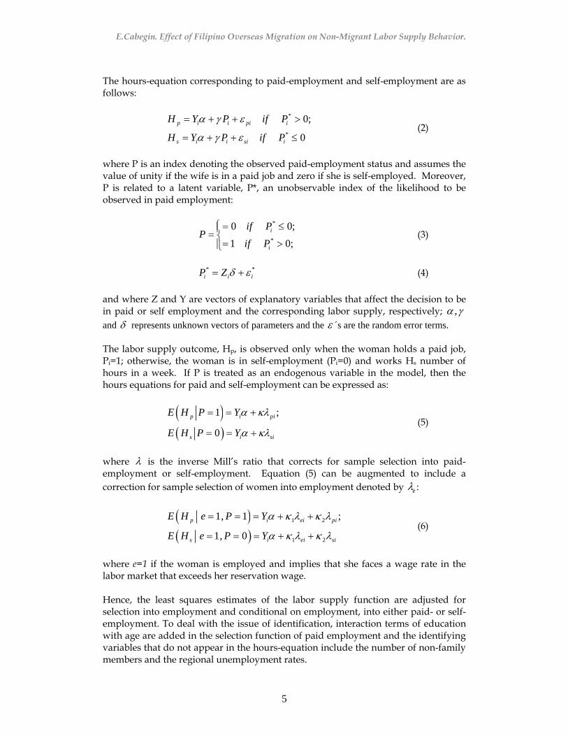
The hours-equation corresponding to paid-employment and self-employment are as follows:

*

*

0;

0p i i pi i

s i i si i

H Y P if P

H Y P if P

α γ ε

α γ ε

= + + >

= + + ≤ (2)

where P is an index denoting the observed paid-employment status and assumes the value of unity if the wife is in a paid job and zero if she is self-employed. Moreover, P is related to a latent variable, P*, an unobservable index of the likelihood to be observed in paid employment:

*

*

0 0;

1 0;i

i

if PP

if P

⎧= ≤⎪= ⎨= >⎪⎩

(3)

* *

i i iP Z δ ε= + (4)

and where Z and Y are vectors of explanatory variables that affect the decision to be in paid or self employment and the corresponding labor supply, respectively; ,α γ and δ represents unknown vectors of parameters and the ε ´s are the random error terms. The labor supply outcome, Hp, is observed only when the woman holds a paid job, Pi=1; otherwise, the woman is in self-employment (Pi=0) and works Hs number of hours in a week. If P is treated as an endogenous variable in the model, then the hours equations for paid and self-employment can be expressed as:

( )( )

1 ;

0

p i pi

s i si

E H P Y

E H P Y

α κλ

α κλ

= = +

= = + (5)

where λ is the inverse Mill’s ratio that corrects for sample selection into paid-employment or self-employment. Equation (5) can be augmented to include a correction for sample selection of women into employment denoted by eλ :

( )( )

1 2

1 2

1, 1 ;

1, 0p i ei pi

s i ei si

E H e P Y

E H e P Y

α κ λ κ λ

α κ λ κ λ

= = = + +

= = = + + (6)

where e=1 if the woman is employed and implies that she faces a wage rate in the labor market that exceeds her reservation wage. Hence, the least squares estimates of the labor supply function are adjusted for selection into employment and conditional on employment, into either paid- or self-employment. To deal with the issue of identification, interaction terms of education with age are added in the selection function of paid employment and the identifying variables that do not appear in the hours-equation include the number of non-family members and the regional unemployment rates.


6

The explanatory variables of interest are interacted with the migration dummy variable to test whether their effects on the labor supply differs for migrant and non-migrant households. For those holding a paid job, for example, an elaborate expression of Equation (6) using pooled data of migrant and non-migrant households is:

( ) 20 1 2 1 11 12

13 1 2

21 22 23

2 1 2

1, 1 06 714

1524 ( * )( 06 * ) ( 714 * ) ( 1524 * )

( * )

p i i i

i si i i i

i i i i i i

si i ei pi

E H e P A A Col C C

C E R M Col MC M C M C ME M

α α α β ϕ ϕ

ϕ δ ψ η βϕ ϕ ϕδ κ λ κ λ

= = = + + + + + +

+ + + + ++ + +

+ +

(7)

where A is age in years; Col is a dummy variable for college education; C06 represents the number of preschool-age children, C714, the number of school-age children and C1524, the number of young working-age children; Es and M are as previously defined and R is a vector of all other variables in Equation (1).

In the above equation, the marginal effect of having a college education on the number of hours worked is represented by 1β for non-migrants and 1 2β β+ for migrants. Hence, 2β indicates the extent to which the marginal effect of having a college education on labor supply differs for migrant and non-migrant households. Similarly, the coefficient 21φ is the difference in the marginal effect of a unit-change increase in the number of preschool children between migrant and non-migrant households.

2.2 Multinomial Probit Model of Labor Force Participation and Supply An alternative econometric specification that allows for richer analysis of the moves between non-participation and self- and paid employment as well as part-time and full-time employment is the multinomial probit model (MNP). For computational tractability of the MNP model, the labor supply is defined in discrete states so that H has three categories as follows: (1) non-employment; (2) part-time employment; and (3) full-time employment. Full-time employment is equivalent to working at least 8 hours a day and part-time employment to working for fewer hours. Non-employment indicates zero hours of work. A more elaborate variant of the different labor supply states further classifies part-time and full-time employment into self-employment and paid employment, leading to five independent employment states:

12 ,3 ,4 ,5 ,

if nonemployedif in part time self employment

H if in full time self employmentif in part time paid employmentif in full time paid employment

⎧⎪ − −⎪⎪= − −⎨⎪ − −⎪

− −⎪⎩


7

If J denotes the different employment alternatives and Uj the level of utility of occupying state j, the unconditional utility maximization problem across the different states is given by:

* max ( )j jU U= , where j = 1,……,J (8) where U* is the maximal utility that an individual can attain. In general, utility maximization will generate a choice of state j if the expected utility, Uj exceeds the expected utility of alternative r, Ur, where r denotes the elements of the set of alternative choices.

max( ) ( ),j j rU U U r j⇔ > ∀ ≠ (9)

Although the utility levels are unobservable, the final labor force participation-

supply state of the wife can be observed, which corresponds to*jU , or the maximum

utility over the set of alternatives. Denote the observed choice as jy

*1,

0,j

j

if Uy

if otherwise

⎧⎪= ⎨⎪⎩

(10)

Suppose Uj is a linear combination of observed individual and household characteristics and a random component as follows:

j j jU Vδ µ= + (11)

where V is a vector of individual and household variables identified in the RHS of Equation (1), δ the vector of corresponding parameters to be estimated and µ the error term. Then the solution to the maximization problem gives the probability of selecting state j (pj):

( )( )( )

Pr , , , 1,....,

Pr , , ,

Pr ,

j j j r r

rj rj rj r j jr j r

rj rj

p V V r j where r j J

V r j where

V r j

δ µ δ µ

µ δ µ µ µ δ δ δ

µ δ

= + > + ∀ ≠ =

= − > ∀ ≠ = − = −

= < ∀ ≠

(12)

If the error terms, rjµ , follow a multivariate normal distribution, then pj is given by:

1

1 1( ,......, ) .....j jJV V

j j Jj j jJp f d dδ δ

µ µ µ µ−∞ −∞

= ∫ ∫ (13)

where f(.) is the normal density function (Maddala, 1983).


8

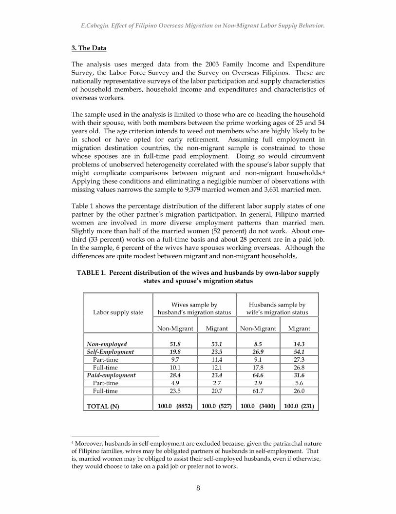
3. The Data The analysis uses merged data from the 2003 Family Income and Expenditure Survey, the Labor Force Survey and the Survey on Overseas Filipinos. These are nationally representative surveys of the labor participation and supply characteristics of household members, household income and expenditures and characteristics of overseas workers. The sample used in the analysis is limited to those who are co-heading the household with their spouse, with both members between the prime working ages of 25 and 54 years old. The age criterion intends to weed out members who are highly likely to be in school or have opted for early retirement. Assuming full employment in migration destination countries, the non-migrant sample is constrained to those whose spouses are in full-time paid employment. Doing so would circumvent problems of unobserved heterogeneity correlated with the spouse’s labor supply that might complicate comparisons between migrant and non-migrant households.4 Applying these conditions and eliminating a negligible number of observations with missing values narrows the sample to 9,379 married women and 3,631 married men. Table 1 shows the percentage distribution of the different labor supply states of one partner by the other partner’s migration participation. In general, Filipino married women are involved in more diverse employment patterns than married men. Slightly more than half of the married women (52 percent) do not work. About one-third (33 percent) works on a full-time basis and about 28 percent are in a paid job. In the sample, 6 percent of the wives have spouses working overseas. Although the differences are quite modest between migrant and non-migrant households,

TABLE 1. Percent distribution of the wives and husbands by own-labor supply states and spouse’s migration status

Wives sample by husband’s migration status

Husbands sample by

wife’s migration status

Labor supply state

Non-Migrant

Migrant

Non-Migrant

Migrant Non-employed

51.8

53.1

8.5

14.3

Self-Employment 19.8 23.5 26.9 54.1 Part-time 9.7 11.4 9.1 27.3 Full-time 10.1 12.1 17.8 26.8 Paid-employment 28.4 23.4 64.6 31.6 Part-time 4.9 2.7 2.9 5.6 Full-time 23.5 20.7 61.7 26.0 TOTAL (N)

100.0 (8852)

100.0 (527)

100.0 (3400)

100.0 (231)

4 Moreover, husbands in self-employment are excluded because, given the patriarchal nature of Filipino families, wives may be obligated partners of husbands in self-employment. That is, married women may be obliged to assist their self-employed husbands, even if otherwise, they would choose to take on a paid job or prefer not to work.


9

there is some indication that wives of migrant husbands are less likely to work, and when they do work, are more likely to be self-employed than wives in non-migrant households. The difference in employment patterns between migrant and non-migrant households is more marked for married men. Husbands of migrant wives are more likely to be non-employed or self-employed and less likely to hold a full-time paid job than those in non-migrant households. Table 2 presents summary statistics for the explanatory variables by spouse’s migration status. Women in migrant households are slightly older and much better educated than their non-migrant counterpart. Less variation in age and education is observed among married men. Migrant households have more children in the working ages and less in children in the younger age groups than non-migrant households. Non-migrant households have less other adult family members but this is true only for women sample. Women in migrant households are more likely to be urban residents than those in non-migrant households, but men in migrant households are more likely to be rural dwellers than their non-migrant counterpart. There is a substantial increase in the husband’s earnings contribution to household income associated with migration, which is over thrice as much in migrant than in non-migrant households. The higher spouse income and non-wage income in migrant relative to non-migrant households is less pronounced in the husband sample.

TABLE 2. Descriptive Statistics

Wives sample by

husband’s migration status

Husbands sample by

wife’s migration status

Variable

Non-Migrant

Migrant

Non-Migrant

Migrant Age 37.02 38.64 40.49 40.27 College education 0.30 0.62 0.39 0.32 N Preschool Age (<7) Children 1.01 0.80 0.76 0.42 N School-age (7-14) Children 1.28 1.10 1.22 1.04 N Young Working age (15-24) Children 0.70 0.98 0.76 0.90 N other adult female members 0.13 0.39 0.21 0.23 N other adult male members 0.08 0.15 .10 0.11 Urban residence 0.56 0.74 0.56 0.40 Spouse’s earnings contribution (0000) 6.76 23.55 7.10 9.57 Non-wage percentile income rank 50.1 86.1 50.62 69.03


10

4. Estimation results 4.1 Switching Regression Model of Labor Force Participation and Supply Table 3 presents the results of the hours-regression model for paid- and self-employment, along with the estimates on the selection equations of working and of holding a paid job, conditional on employment. The coefficients of the conventional variables generally confirm findings of previous work on married women’s labor supply and are in line with theoretical expectations. The coefficient for the age variable indicates that, even after controlling for other relevant factors, the participation of married women in the labor market increases up to a threshold level and then declines thereafter. However, conditional on employment, age does not significantly affect married women’s labor supply or the choice between a paid job and self-employment. For married men, age does not figure significantly in market participation but for those who do work, they are less likely to hold a paid job than be self-employed as they advanced in age after a certain age threshold. The presence of another female adult member is associated with higher market participation, and more particularly in paid employment than in traditional self-employment. Urban residents are less likely to be employed (but significantly so only for married men) and for those employed, are more likely to hold a paid job than be self-employed and also more likely to work longer hours. As expected, a higher regional unemployment rate discourages market participation. The coefficient of the sample-selection correction factors in the work hours-equation is not significant in the case of married women. The significant and negative inverse mills ratio for married men indicates the presence of unobserved characteristics increasing the likelihood of employment that are inversely related to the hours of work decision. The presence of young children impacts prominently on the labor participation and supply decision of married women, with varying effects by age of children and spouse’s migration status. The strong effect of young children on market participation is largely absent for men. However, for men who do work, there is indication of some children effects on the decision to take on a paid job or on the labor supply. Having a child in the pre-school age (< 7 years old) significantly discourages married women in non-migrant households from market participation particularly from paid employment, with the effect not significantly different from that of migrant households. Preschool age children do not appear to affect significantly the labor supply among working women nor in the market participation and labor supply for married men. The presence of school-age (7-14 years old) children increases the likelihood to work among women in non-migrant households while having the reverse effect for migrant households. School-age children do not appear to affect significantly the choice between paid work and self-employment among working women in non-migrant households. Conditional on employment, women in non-migrant households with school-age children are less likely to work longer hours particularly if they are holding a paid job. Married women in migrant households with


11

TABLE 3. Switching Regression Model on Employment States and Hours Worked (Wife Sample)

Probit Results On:

Selection-Corrected OLS on Hours Worked§

Model 3.1

Employment

Model 3.2 Paid Work Conditional

on Employment

Model 3.3

Employed Sample

Model 3.4

Paid-Employed Sample

Model 3.5

Self-Employed Sample

Variable

Coefficient z-stat Coefficient z-stat Coefficient t-stat Coefficient t-stat Coefficient t-stat Age 0.1244*** 6.24 -0.0016 -0.04 -0.0165 -0.26 -0.0416 -0.72 0.0407 0.29 Age squared -0.0014*** -5.57 0.0000 -0.02 0.0003 0.33 0.0004 0.58 -0.0002 -0.12 College graduate 0.2772*** 5.56 0.8161 0.68 0.2493 1.56 -0.0528 -0.34 0.5304 1.38 N Preschool Age (<7) Children -0.1966*** -10.31 -0.0653** -2.08 -0.0983 -1.27 0.0020 0.03 -0.1369 -0.87 N School-age (7-14) Children 0.0568*** 3.76 0.0318 1.40 -0.1038** -2.29 -0.1410*** -3.42 -0.0912 -1.04 N Young Working age (15-24) Children -0.0214 -1.16 0.1218*** 4.35 -0.0047 -0.09 -0.0065 -0.14 -0.0592 -0.53 N other adult female members 0.2935*** 8.39 0.3324*** 7.00 N other adult male members -0.0430 -1.03 0.1879*** 3.06 Urban -0.0471 -1.55 0.1723*** 3.96 0.4414*** 5.05 0.0661 0.74 0.7948*** 4.02 Predicted Husband’s earnings♣ -0.0040 -0.57 0.0060 0.59 -0.0221 -1.18 -0.0222 -1.53 -0.0299 -0.86 Non-wage income -0.0004 -0.63 -0.0213*** -23.54 0.0081*** 5.31 0.0068** 2.16 0.0232** 2.54 Migrant husband (Mig) 0.2119 0.32 4.6322*** 4.45 0.6138 0.35 -1.5829 -0.91 2.5047 0.58 College*Mig 1.8482*** 3.65 2.0865** 2.53 0.0964 0.06 -0.2802 -0.19 0.8167 0.27 N Preschool*Mig 0.2373 1.06 -0.2101 -0.56 0.3129 0.52 0.0020 0.00 0.1618 0.10 N SchoolAge*Mig -0.7395*** -4.03 -0.9238*** -3.19 0.4740 1.02 0.7122** 2.01 0.3914 0.34 N Working Age*Mig -0.1331 -0.55 -1.4193*** -3.85 -0.5756 -0.94 0.1994 0.45 -1.6627 -1.18 H Earnings*Mig -0.0639 -1.49 -0.1590** -2.31 0.0050 0.04 0.1369 1.44 -0.1543 -0.69 Regional unemployment rates -3.4655*** -7.4 Selection factor-Employment 0.2193 0.61 0.4430 1.3 -0.1977 -0.22 Selection factor-Paid employment 0.2446 0.81 Selection factor-Self employment 0.3626 0.52 Age-Education Dummy Interaction Yes No No No Constant -2.1754*** -5.81 0.7825 1.11 7.3438*** 5.27 9.0570*** 7.65 4.4175 1.24

♣Husband’s earnings contribution to household income; § Number of normal working hours in a day; *** significant at .01 level; ** significant at .05 level; * significant at .10 level; Diagnostics: Model 3.1: N= 9379; Waldchi2(18)=740.07¸Prob >chi2=0.0; Log likelihood=-6102.29; Pseudo R2=.0603; Model 3.2: N= 4509; Waldchi2(19)=728.98¸Prob >chi2=0.0; Log likelihood=-2633.798; Pseudo R2=.1396; Model 3.3: N= 4509; F(16,4492)=13.41; Prob >F=0.0; R2=.0378; Model 3.4: N= 2634; F(17,2616)=4.94; Prob >F=0.0; R2=.0244; Model 3.5: N= 1874; F(17,1857)=11.42; Prob >F=0.0; R2=.0850;


12

TABLE 4. Switching Regression Model on Employment States and Hours Worked (Husband Sample)

Probit Results On:

Selection-Corrected OLS on Hours Worked§

Model 4.1

Employment

Model 4.2 Paid Work Conditional

on Employment

Model 4.3

Employed Sample

Model 4.4

Paid-Employed Sample

Model 4.5

Self-Employed Sample

Variable

Coefficient z-stat Coefficient z-stat Coefficient t-stat Coefficient t-stat Coefficient t-stat Age 0.0113 0.24 0.0635 1.36 -0.0079 -0.16 -0.0399 -0.77 -0.02006 -0.18 Age squared -0.0003 -0.52 -0.0010* -1.67 -0.0001 -0.21 0.0004 0.58 -0.00014 -0.11 College graduate 0.1232 1.14 1.3225 0.87 0.2276* 1.82 -0.2452 -1.33 0.5250 0.94 N Preschool Age (<7) Children -0.0655 -1.30 -0.0412 -1.00 0.0153 0.34 0.0076 0.18 0.0654 0.57 N School-age (7-14) Children 0.0452 1.18 -0.0556* -1.86 0.0087 0.25 -0.0334 -0.91 0.1366 1.47 N Young Working age (15-24) Children 0.0036 0.09 0.0908*** 2.81 0.0399 0.92 0.0529 1.17 -0.0253 -0.26 N other adult female members 0.3865*** 5.29 0.2737*** 5.09 N other adult male members -0.0259 -0.31 0.0670 0.92 Urban -0.2795*** -3.76 0.4616*** 8.50 0.2840*** 3.51 0.1369 1.09 0.3263 0.84 Predicted Wife’s earnings♣ -0.0056 -0.41 -0.0101 -0.87 -0.0357** -2.27 -0.0120 -0.72 -0.0667** -2.05 Non-wage income -0.0036*** -2.80 -0.0249*** -21.4 -0.0027** -1.96 0.0022 0.51 0.0029 0.23 Migrant wife (Mig) 0.0978 0.09 -1.2565 -1.27 -2.0053* -1.66 -2.431* -1.77 -1.5044 -0.62 College*Mig 0.2327 0.23 -1.5257* -1.87 0.4193 0.39 2.4446** 2.00 -2.448 -0.95 N Preschool*Mig -0.0398 -0.10 0.5916 1.62 0.4071 0.97 -0.1546 -0.38 1.2591 1.18 N SchoolAge*Mig 0.1613 0.43 0.4357 1.49 0.5643 1.61 0.7416* 1.74 -0.0503 -0.08 N Working Age*Mig 0.8091 1.74 -0.1216 -0.35 -0.2276 -0.4 -0.2627 -0.47 0.3680 0.35 W Earnings*W migrant -0.2782* -1.90 -0.0531 -0.42 -0.1522 -0.94 0.0296 0.14 -0.2776 -0.85 Regional unemployment rates -5.4474*** -5.71 Selection factor-Employment -1.6354*** -3.26 -0.9895* -1.82 -2.5504* -1.75 Selection factor-Paid employment 0.0164 0.04 Selection factor-Self employment 0.2351 0.27 Age-Education Dummy Interaction Yes No No No Constant 2.3124** 2.47 0.4345 0.47 8.4976 8.89 9.1715*** 8.94 8.2903*** 3.38

♣Wife’s earnings contribution to household income; § Number of normal working hours in a day; *** significant at .01 level; ** significant at .05 level; * significant at .10 level; Diagnostics: Model 4.1: N= 3631; Waldchi2(18)=137.62¸Prob >chi2=0.0; Log likelihood=-1016.41; Pseudo R2=.0653; Model 4.2: N= 3309; Waldchi2(19)=616.13¸Prob >chi2=0.0; Log likelihood=-1695.044; Pseudo R2=.1768; Model 4.3: N= 3309; F(16,3292)=6.64; Prob >F=0.0; R2=.0340; Model 4.4: N= 2270; F(17,2252)=2.50; Prob >F=0.0; R2=.0199; Model 4.5: N= 1039; F(17,1021)=3.83; Prob >F=0.0; R2=.0547.

E.Cabegin. Effect of Filipino Overseas Migration on Non-Migrant Labor Supply Behavior

13

school-age children are significantly less likely to hold a paid job than their non-migrant counterpart, but conditional on paid employment are more likely to work longer. For married men, school age children do not affect significantly market participation decision but reduces the likelihood of taking a paid job among those who are working, with no significant difference observed between migrant and non-migrant households. For men in paid employment, having school-age children is associated with higher labor supply for those with migrant wives. Children in the young working ages of 15 to 24 do not affect significantly the employment decision of married men and women. However, conditional on working, those with older children are more likely to be in paid than in self-employment for married men and for married women in non-migrant households. The reverse pattern is observed for women in migrant households, where the presence of older children is associated with a higher likelihood to be self-employed than to hold a paid job. The labor force supply behavior appears to be independent of the number of family members in the young working age below 25 years old. Given that employers do not discriminate according to their spouse’s migration status (as this information is usually not known by the employer), then those with equivalent market productivity characteristics are expected to earn similar wages. Thus controlling for age and all other pertinent factors that affect the value of home time, varied effects of a given level of education on employment choices between migrant and non-migrant households reflects indirectly the effect of spouse’s leisure time at home on own-time for household care. Note that in migrant households, the spouse’s leisure time at home is zero, reducing the gains from specialization in home production particularly in households with no children. If the husband’s leisure time at home is complementary with the wife’s housework time as seems to be the case in the Philippines, then the husband’s migration is expected to raise the wife’s propensity for market participation. An alternative interpretation of the differences in labor supply behavior of those with equivalent levels of human capital between migrant and non-migrant households is that remittances in migrant households can act as an insurance mechanism whereby families in the sending country are provided a financial guarantee to achieve a certain standard of living, regardless of the work effort levels of the other household members [Lipton, 1980]. Some studies have attributed this reduction in market work to a moral hazard problem where higher remittance income is purported to induce a sense of dependency by the migrant’s family [Chami, R., C. Fullenkamp and S. Jahjah, 2003]. However, this assertion is justified if market work is substituted for idleness rather than an increase in household and child care by those whose spouses have migrated. Indicative of the higher opportunity cost of non-employment, married women who are college-educated are much more likely to participate in the labor force, with stronger effects observed for migrant than non-migrant households. Working married women in migrant households with a college education are also more likely to be in paid employment than similarly categorized women in non-migrant households. College education has no significant effect on married women’s labor supply behavior.


14

For working married men, college education is associated with higher likelihood of being self-employed than taking on a paid job but only for migrant households. For non-migrant households, the effect of a college education is positive but not significant in the choice of paid employment. Those with a college education are also more likely to work longer hours than their less educated counterpart with no significant difference between migrant and non-migrant households. The husband’s earnings contribution to household income does not affect significantly the wife’s market participation or labor supply regardless of migration status. However, conditional on working, higher husband’s earnings contribution is associated lower propensity of wives in migrant households to hold a paid job than to be self-employed. The effect of the wife’s earnings contribution to household income on their husband’s employment decision is not significant for non-migrant households but negative and significant for migrant households. 4.2 Multinomial probit model of husband migration-wife labor participation and

supply This section discusses the MNP models on the labor force participation and supply states of married men and women using pooled sample of migrant and non-migrant households. To test the statistical significance of the effect of the migration status, the model includes explanatory variables that are interacted with migration status. Tables 4 and 5 presents the difference in the marginal effect of a variable on the labor participation and supply outcomes between migrant and non-migrant households and a formal test on whether the difference in the response is statistically significant.5 Pre-school-age children are associated with lower market participation of married women for all forms of employment, with no significant difference between migrant and non-migrant households. A child in the preschool age is associated with an 8 percent increase in the probability of non-employment among married women. For married men, the overall effect on non-employment is not significant but there is indication of a negative significant effect on part-time self-employment for migrant households and on part-time paid employment for non-migrant households. Wives with school-age (7-14 years old) children are significantly less likely to work if their husbands have migrated and more likely to work if they are in non-migrant households. Wives in migrant households are less likely to take on a full-time paid job while similarly categorized women in non-migrant households are more likely to participate in paid employment. Women with school-age children switch from full-time paid employment to non-employment in migrant households and from non-employment to paid employment in non-migrant households. The test of differential

5 Appendices C and D present the estimates of the full model for both husband and wives with non-employed persons as the reference category.


15

TABLE 7. Marginal effects of Children Variables On Labor Participation and Supply

*** significant at .01 level; ** significant at .05 level; * significant at .10 level effects of this variable by migration status indicate that women in migrant households with a school-age child are 28 percent less likely than non-migrant households to be holding a full-time paid job and 26 percent more likely to be non-employed than women in non-migrant households. Among married men, the effect of school age children on non-employment is negative but not significant, but positive and significant for full-time self-employment in non-migrant households and full-time paid employment in migrant households. The presence of children in the young working age (15-24 years old) is associated with significant shifts from self-employment to paid employment in non-migrant households. Married women in migrant households with a child in the young working age are 12 percent more likely to be self-employed on a part-time basis but 19 percent less likely to take a full-time paid job than those in non-migrant households. For married men, a child in the young working age is associated with a shift from full-time self-employment to full-time paid employment with no significant difference between migrant and non-migrant households. The likelihood of holding a paid job on a part-time basis among married men with a working-age child is higher by 7 percent in non-migrant households.

Wife Sample

Husband Sample

Non-Migrant Households

Difference Between Migrant and Non-

Migrant HHs



Migrant HHs

Employment State

Parameter

z-stat

Parameter

z-stat

Parameter

z-stat

Parameter

z-stat

Preschool Children

Non-employment 0.0783*** 10.25 -0.1056 -1.16 0.0117 1.48 -0.0294 -0.43 Self-Employment, Part-Time -0.0094** -2.06 0.0700 1.20 0.0065 0.80 -0.1868** -2.24 Self-Employment, Full-Time -0.0142*** -3.14 0.0633 1.20 0.0025 0.23 0.0004 0.00 Paid-Employment, Part-Time -0.0093*** -3.43 0.0389 1.00 -0.0107** -2.02 0.0573 1.37 Paid-Employment, Full-Time -0.0453*** -6.73 -0.0665 -0.87 -0.0100 -0.72 0.1585 1.23

School-Age Children Non-employment -0.0211*** -3.50 0.2616*** 3.56 -0.0066 -1.09 -0.0385 -0.65 Self-Employment, Part-Time 0.0017 0.49 0.0219 0.48 -0.0012 -0.22 -0.0597 -1.29 Self-Employment, Full-Time -0.0018 -0.51 0.0319 0.74 0.0202*** 2.64 -0.0889 -1.21 Paid-Employment, Part-Time 0.0093*** 4.32 -0.0367 -1.19 -0.0035 -0.94 0.0123 0.42 Paid-Employment, Full-Time 0.0118*** 2.32 -0.2787*** -4.51 -0.0089 -0.87 0.1748* 1.75

Young Working Age Children Non-employment 0.0090 1.23 0.0330 0.34 -0.0012 -0.20 -0.1182 -1.59 Self-Employment, Part-Time -0.0099** -2.34 0.1234** 2.26 -0.0070 -1.18 0.0393 0.70 Self-Employment, Full-Time -0.0158*** -3.82 0.0884 1.61 -0.0237*** -2.81 0.0492 0.55 Paid-Employment, Part-Time 0.0050* 1.85 -0.0523 -1.2 -0.0044 -1.13 0.0709* 1.85 Paid-Employment, Full-Time 0.0117* 1.91 -0.1926** -2.38 0.0363*** 3.27 -0.0413 -0.32


16

Women with a college education are significantly more likely to be employed and particularly on a full-time paid job, with much stronger effects for migrant than non-migrant households. The negative effect of a college education on non-emplyoment is 71 percent larger in migrant households and its positive effect on full-time paid employment is 59 percent higher. This indicates complementarity of husband’s leisure time with the wife’s home time. Attainment of college education has no significant effect on overall non-employment among married men but induces significant shifts occurring from self-employment to full-time paid employment for non-migrant households. A reverse pattern is indicated for married men in migrant households although the coefficients did not turn out to be significantly different from that of non-migrant households. An increase in husband’s earnings contribution to household income has no significant effect on employment patterns of women in non-migrant households. However, an annual increase of 10,000 pesos in husband’s earnings contribution to household income reduces the likelihood of wives in migrant households to hold a full-time paid job by 4 percent relative to non-migrant households. Stronger income effects are observed for married men. The higher the remittance income of the migrant wife is associated with lower the likelihood of the husband’s market participation. For non-migrant households, the higher wife’s earnings contribution to household income is associated with shifts away from full-time to part-time self-employment. The pattern observed in migrant households is a switch from full-time to part-time paid employment and to a larger extent to non-employment. An increase of wife’s earnings contribution to household income by 10,000 pesos a year is associated with a 12 percent lower likelihood of husbands in migrant households than in non-migrant households to take on a full-time paid job and a 6 percent higher likelihood to be non-employed.

TABLE 7. Marginal effects of Education and Income Variables On

Labor Participation and Supply

*** significant at .01 level; ** significant at .05 level; * significant at .10 level

Wife Sample

Husband Sample



Migrant HHs



Migrant HHs

Employment State

Parameter

z-stat

Parameter

z-stat

Parameter

z-stat

Parameter

z-stat

College Education

Non-employment -0.1272*** -6.49 -0.7193*** -3.55 -0.0245 -1.51 -0.0729 -0.44 Self-Employment, Part-Time -0.0428*** -3.78 -0.0246 -0.19 -0.0913*** -6.90 0.2086 1.56 Self-Employment, Full-Time -0.0355*** -3.38 0.1109 0.94 -0.1262*** -6.35 0.1400 0.70 Paid-Employment, Part-Time 0.0042 0.51 0.0446 0.52 0.0079 0.75 -0.1039 -1.14 Paid-Employment, Full-Time 0.2014*** 11.53 0.5884*** 3.39 0.2341*** 8.48 -0.1719 -0.61

Spouse’s Earnings Contribution to HH Income Non-employment 0.0031 1.14 0.0181 1.09 0.0005 0.23 0.0615*** 2.64 Self-Employment, Part-Time -0.0014 -0.85 0.0168 1.63 0.0050** 2.55 0.0084 0.41 Self-Employment, Full-Time -0.0023 -1.43 -0.0030 -0.29 -0.0058** -1.96 0.0194 0.61 Paid-Employment, Part-Time -0.0005 -0.48 0.0037 0.59 -0.0009 -0.70 0.0296** 2.16 Paid-Employment, Full-Time 0.0011 0.48 -0.0356*** -2.57 0.0012 0.30 -0.1189*** -2.58


17

5. Conclusion The estimates indicate that for married couples, the participation in overseas migration of one partner significantly modifies the labor participation and supply behavior of the other partner but this operates through different mechanisms for married men and women. In particular, estimates establish stronger conjugal home time effects of migration for married women and larger remittance income effects for married men. The presence of school-age children is associated with higher market participation of women in non-migrant households particularly in part-time paid employment while having the reverse effect for women in migrant households particularly in respect to full-time paid employment. Women in migrant households with a school-age child are 28 percent less likely than non-migrant households to be holding a full-time paid job and 26 percent more likely to be non-employed than women in non-migrant households. The presence of children in the young working age is associated with a switch from self- to paid employment among women in non-migrant households and the reverse pattern for migrant households. Married women in migrant households with a child in the young working age are 12 percent more likely to be self-employed and 19 percent less likely to take on a full-time paid job than those in non-migrant households. The attainment of a college education induces a shift away from non-employment and towards full-time paid employment with much stronger effects for women in migrant than in non-migrant households. The effect of a college education is 71 percent more negative on non-employment for migrant than non-migrant households and 59 percent more positive in respect to full-time paid employment. This indicates complementarity of husband’s leisure time with the wife’s time in household production, so that the migration of the husband frees up time for the wife in favor for market work. While children effects on labor participation and supply behavior are weaker among married men, the income remittance effects are stronger. The higher remittance income of the migrant wife is associated with lower likelihood of husband’s market participation particularly in full-time paid employment. An annual increase of wife’s earnings contribution to household income by 10,000 pesos reduces the likelihood of taking on a full-time paid job by 12 percent more and increases the likelihood of non-employment by 6 percent higher in migrant than in non-migrant households.


18

Appendix A: Regression model on (ln) husband’s earnings contribution to HH income

Husband’s Earnings Contribution to HH

Income Wife’s Earnings Contribution to HH Income

Model A.1 Non-Migrant

Model A.2 Migrant

Model A.3 Non-Migrant

Model A.4 Migrant

Variable

Coefficient t-stat Coefficient t-stat Coefficient t-stat Coefficient t-stat Age 0.0216*** 3.29 0.0951* 1.75 -0.0139 -1.26 -0.1299 -1.18 Age squared -0.0002** -2.50 -0.0094 -1.38 0.0002* 1.67 0.0019 1.32 High school graduate 0.1799*** 15.15 0.1737 1.49 0.2017*** 6.91 0.4182** 2.36 Some college education 0.2563*** 15.83 0.3787*** 3.37 0.3925*** 9.48 0.6234*** 3.25 College graduate 0.6223*** 25.58 0.6396*** 5.46 0.7113*** 15.02 0.6734*** 3.17 Occupation_1 0.4894*** 16.75 0.7803*** 11.96 0.0610 1.41 Occupation_2 0.3712*** 10.12 0.7294*** 9.49 -0.5398 -0.85 Occupation_3 0.3641*** 6.94 0.6495*** 11.59 0.3826 0.88 Occupation_4 0.3655*** 12.04 0.7473*** 15.80 0.6417*** 2.82 Occupation_5 0.4229*** 10.97 0.7403*** 12.77 0.2183* 1.74 Occupation_6 0.0668** 2.30 0.3509*** 8.04 3.2970 1.60 Occupation_7 -0.4701*** -25.91 -0.1964*** -7.67 Occupation_8 0.0305* 1.82 0.1701*** 3.50 Occupation_9 0.1377*** 6.83 0.6326*** 10.98 Occupation_10 0.0226 0.83 0.2549*** 6.72 Occupation_11 0.0643*** 3.37 Years worked overseas 0.0394** 1.98 0.0610 1.41 Occupation overseas_1 0.2508*** 2.90 -0.5398 -0.85 Destination_1 0.2138** 2.59 0.3826 0.88 Destination_2 0.2509*** 3.08 0.6417*** 2.82 Constant 1.0128*** 7.94 -1.218 -0.11 0.2183* 1.74 1.1833*** 5.59 3.2970 1.60

*** significant at .01 level; ** significant at .05 level; * significant at .10 level. Diagnostics: Model A.1: N=8852; R-squared: .4725; F(16, 8835) =570.91; Prob>F=0.0; Model A.2: N=527; R-squared: .2153; F(9,517)=15.01; Prob>F=0.0; Model A.3: N=3400; R-squared: .6503; F(15, 3384) =785.07; Prob>F=0.0; Model A.4: N=231; R-squared: .1916; F(10,220)=6.23; Prob>F=0.0.


19

Appendix B: Regression Model on Husband’s Migration Status

Probit on Migration Status

Model B.1 Husband Model B.2 Wife

Variable Coefficient t-stat Coefficient t-stat Age 0.1537*** 4.26 0.1826*** 3.10 Age squared -0.0021*** -4.65 -0.0028*** -3.62 High school graduate 0.5011*** 6.40 0.7697*** 7.31 Some college 0.9973*** 12.98 0.9192*** 7.21 College graduate 1.2441*** 15.71 -0.0440 -0.42 Occupation_1 0.2194** 2.24 -0.6321*** -5.78 Occupation_2 0.1244* 1.71 -0.6767*** -4.82 Occupation_3 0.3769*** 4.92 Occupation_4 0.4679*** 3.78 Urban -0.0652 -0.71 -0.2336* -1.88 Manila 0.5083*** 6.02 -0.0363 -0.23 CAR 1.1453** 2.51 -0.2501 -0.39 Ilocos 0.3187 0.88 0.7970* 1.86 Central Luzon 0.6228** 2.46 0.2683 0.71 CALABARZON 0.9516*** 4.28 -1.2349*** -2.76 Western Visayas 0.7293** 2.37 0.9304* 1.73 Central Visayas 0.4034 1.22 -0.2834 -0.38 Urban*CAR -0.5969* -1.76 0.3598 1.02 Urban*Ilocos 0.1035 0.48 -0.1273 -0.52 Urban*Central Luzon -0.1015 -0.57 -0.1444 -0.60 Urban*CALABARZON -0.1944 -1.19 0.7977*** 2.89 Urban*Western Visayas -0.1981 -1.02 -0.6080** -1.98 Urban*Central Visayas -0.1246 -0.52 -0.1480 -0.28 Constant -5.3243*** -7.58 -4.4069*** -3.98

*** significant at .01 level; ** significant at .05 level; * significant at .10 level Diagnostics: Model B.1 N=9379; Wald chi2(23) = 565.42; Prob > chi2 = 0.0; Log pseudolikelihood = -1690.433; Pseudo R-squared: .1669; Model B.2 N=3631; Wald chi2(21) = 224.50; Prob > chi2 = 0.0; Log pseudolikelihood = -704.860; Pseudo R-squared: .1803


20

APPENDIX C. MNP Coefficients of Wife’s Labor Participation and Supply §

Self-employment,

Part-Time

Self-employment,

Full-Time

Paid-employment,

Part-Time

Paid-employment,

Full-Time

Variable Coefficient z-stat Coefficient z-stat Coefficient z-stat Coefficient z-stat

Age 0.1703*** 4.58 0.1596*** 4.22 0.1302*** 2.81 0.1515 4.80 Age squared -0.0021*** -4.31 -0.0019*** -3.93 -0.0014** -2.41 -0.0017*** -4.12 College graduate -0.0712 -0.71 -0.0364 -0.37 0.2695** 2.33 0.8021*** 10.94 N Preschool Age (<7) Children -0.1919*** -5.46 -0.2277*** -6.23 -0.2535*** -6.51 -0.2776*** -8.89 N School-age (7-14) Children 0.0469* 1.72 0.0246 0.86 0.1540*** 4.95 0.0736*** 3.09 N Young Working age (15-24) Children -0.0773** -2.34 -0.1200*** -3.54 0.0460 1.18 0.0226 0.78 N adult NF female members 0.1719*** 2.57 0.1299** 2.04 0.0944 0.93 0.5977*** 11.67 N adult NF male members -0.1469* -1.91 -0.1824** -2.41 0.1623* 1.77 0.0046 0.07 Urban residence -0.2425*** -4.33 -0.0243 -0.42 0.0858 1.26 -0.0187 -0.40 Predicted Husband’s earnings -0.0139 -1.11 -0.0203 -1.58 -0.0121 -0.78 -0.0017 -0.17 Non-wage income (Rank) 0.0078*** 7.14 0.0173*** 14.95 -0.0132*** -9.38 -0.0100*** -10.76 Regional unemployment rates -5.7426*** -6.62 -5.6869*** -6.69 -1.5604 -1.43 -3.6873*** -5.01 Migration Status -3.3903*** -2.60 -2.1261* -1.74 -0.9421 -0.65 2.3215** 2.23 College graduate*Mig 1.0660 1.06 1.9498** 2.06 1.7980 1.50 3.1037*** 3.87 N preschool*Mig 0.6195 1.40 0.6052 1.43 0.6826 1.24 -0.0355 -0.10 N School-age*Mig -0.3053 -0.87 -0.2311 -0.67 -0.9070** -2.07 -1.3374*** -4.63 N Young Work Age*Mig 0.7117* 1.69 0.5326 1.19 -0.7032 -1.14 -0.6763* -1.78 Husband’s earnings*Mig 0.0746 0.94 -0.0490 -0.6 0.0171 0.19 -0.1449** -2.26 Constant -3.9151*** -5.59 -4.3321*** -6.05 -3.6919*** -4.22 -3.2451*** -5.44 §Reference Category: Non-employed; *** significant at .01 level; ** significant at .05 level; * significant at .10 level; Diagnostics: N=9379; Wald chi2(72)=1801.26; Prob > chi2 = 0.0; Log pseudolikelihood = -11060.853

APPENDIX D. MNP Coefficients of Husband’s Labor Participation and Supply §

§Reference Category: Non-employed; *** significant at .01 level; ** significant at .05 level; * significant at .10 level; Diagnostics: N=3631; Wald chi2(72)=892.87; Prob > chi2 = 0.0; Log pseudolikelihood = -3782.149

Self-employment,

Part-Time

Self-employment,

Full-Time

Paid-employment,

Part-Time

Paid-employment,

Full-Time

Variable Coefficient z-stat Coefficient z-stat Coefficient z-stat Coefficient z-stat

Age -0.0129 -0.17 .0083 0.12 .0646 0.69 .0426 0.67 Age squared 0.0002 0.19 -0.0002 -0.28 -0.001 -0.88 -0.0008 -1.02 College graduate -0.5342*** -3.10 -0.3648** -2.24 0.2957 1.41 0.5593 3.69 N Preschool Age (<7) Children -0.0361 -0.43 -0.0721 -0.95 -0.2471** -2.41 -0.0976 -1.44 N School-age (7-14) Children 0.0380 0.64 0.1278** 2.29 -0.0073 -0.10 0.0331 0.64 N Young Working age (15-24) Children -0.0407 -0.66 -0.0854 -1.48 -0.0609 -0.80 0.0670 1.28 N adult NF female members 0.2403** 2.05 0.3045*** 2.83 0.4237*** 2.96 0.6524 6.66 N adult NF male members 0.0635 0.47 -0.1951 -1.51 -0.1121 -0.61 0.0201 0.18 Urban residence -0.7083*** -6.04 -0.5412*** -4.98 -0.3322** -2.39 -0.1767 -1.77 Predicted Wife’s earnings 0.0318 1.48 -0.0272 -1.31 -0.0181 -0.68 -0.0019 -0.10 Non-wage income (Rank) 0.0122*** 5.36 0.0166*** 8.02 -0.0119*** -4.12 -0.0171 -9.04 Regional unemployment rates -10.8646*** -6.65 -9.9846*** -6.77 -4.4695** -2.24 -4.5894 -3.50 Migration Status 1.6358 0.93 0.4597 0.27 -3.2789 -1.48 -0.0999 -0.06 College graduate*Mig 1.9774 1.30 1.0741 0.72 -1.0888 -0.59 0.2458 0.17 N preschool*Mig -1.1058 -1.39 0.2146 0.33 1.0844 1.32 0.4610 0.78 N School-age*Mig -0.1485 -0.28 -0.0816 -0.15 0.4512 0.72 0.5501 1.07 N Young Work Age*Mig 1.1065* 1.67 1.0264 1.56 1.9300** 2.39 0.7610 1.16 Wife’s earnings*Mig -0.3730* -1.77 -0.3599* -1.68 0.0332 0.12 -0.6267 -2.98 Constant 1.0405 0.68 1.2129 0.86 -0.0028 0.00 2.3029 1.83


21

R e f e r e n c e s

Angrist, J. D. andW. N. Evans. 1996. “Children and Their Parents’ Labour Supply:

Evidence from Exogenous Variation in Family Size”, National Bureau of Economic Research (Cambridge, MA, U.S.A.) Working Paper No. 5778.

Asian Development Bank. 2004. ““Enhancing the efficiency of Overseas Filipino

Workers’ Remittances,” ADB Manila. Cabegin, E. 1996. “The Value of Non-Market Household Production in Filipino

Households.” Mimeograph. Chami, R., C. Fullenkamp, and S. Jahjah. 2003. "Are Immigrant Remittance Flows a

Source of Capital for Development?" IMF Working Paper No. 03/189 Domingo, L, C. Raymundo and E. Cabegin. 1994. “Conjugal Division of Labor in

Employment, Housework and Child Care in the Philippines.” Mimeograph.

Heckman, J. 1979. “Sample Selection Bias as A Specification Error.” Econometrica. 47: 153-161.

Lipton, M. 1980. "Migration from rural areas of poor countries: the impact on rural

productivity and income distribution". World Development. Vol. 8:1-24. Maddala, G.S. 1983. Limited-Dependent and Qualitative Variables in

Econometrics. Econometric Society Monographs in Quantitative Economics. Cambridge, Cambridge University Press.

Orbeta, A. 2005. “Children and Labor Force Participation and Earnings of Parents in

the Philippines.” ADB Institute Discussion Paper No. 30. Philippine Overseas Employment Administration. 2006. Tables on the number of

deployed overseas Filipino workers: 1998-2005 and stock estimates of overseas Filipinos as of December 2004. http: //www.poea.gov.ph/ stats/ 2005deployment.xls

Rosenzweig, M. and K. Wolpin. 1980. “Testing the Quantity-Quality Fertility Model:

The Use of Twins as a Natural Experiment”, Econometrica 48(1): 227-240. Stark, O. 1991. Migration of Labor. Cambridge: Basil Blackwell. World Bank. 2005. “Global Economic Prospects 2006: Economic Implications of

Remittances and Migration”, WB: Washington, D.C.

The Effect of Filipino Overseas Migration on the Non ...ftp.iza.org/dp2240.pdf · The Effect of...

Documents

Transcript of The Effect of Filipino Overseas Migration on the Non ...ftp.iza.org/dp2240.pdf · The Effect of...