The E ect of Occupational Licensing Stringency on the ...

The Effect of Occupational Licensing Stringency on the Teacher

Quality Distribution*,†

Bradley J. Larsen1,3, Ziao Ju1, Adam Kapor2,3 and Chuan Yu1

1Department of Economics, Stanford University2Department of Economics, Princeton University

3NBER

December 2, 2020

Abstract

Concerned about the low academic ability of public school teachers, in the 1990s and 2000s, somestates increased licensing stringency to weed out low-quality candidates, while others decreased restric-tions to attract high-quality candidates. We offer a theoretical model justifying both reactions. Usingdata from 1991–2007 on licensing requirements and teacher quality—as measured by the selectivity ofteachers’ undergraduate institutions—we find that stricter licensing requirements, especially those em-phasizing academic coursework, increase the left tail of the quality distribution for secondary schoolteachers without significantly decreasing quality for high-minority or high-poverty districts.

Keywords: Teacher licensing, teacher certification, teacher quality, education, occupational licensing

JEL Classification: I2, J2, J4, J5, K2, K31, L5, L8

*This paper replaces an earlier working paper (Larsen 2015) circulated under the title “Occupational Licensing and Quality:Distributional and Heterogeneous Effects in the Teaching Profession.” We thank Mike Abito, Josh Angrist, David Autor, PanleJia Barwick, Brant Callaway, Sarah Cohodes, Ignacio Cuesta, Clement de Chaisemartin, Daniel Goldhaber, Jon Guryan, EricHanushek, David Harrington, Michael Hartney, Caroline Hoxby, Sally Hudson, Lisa Kahn, Morris Kleiner, Matt Kraft, KatieLarsen, Christopher Palmer, Jesse Rothstein, Nicholas Rupp, Pedro H. C. Sant’Anna, Philip Solimine, John Tyler, Chris Walters,and Frank Wolak, as well as seminar participants at Brown University, MIT, Stanford, Texas A&M University, the 2014 Interna-tional Industrial Organization Conference, the 2015 NBER Law and Economics Winter Meetings, the 2016 AEA Meetings, theU.S. Department of Labor Employment and Training Administration, and the 2020 Knee Center Occupational Licensing Confer-ence for helpful comments and suggestions. We also thank Josh Angrist, Brigham Frandsen, Jon Guryan, Andrew Hall, MindyMarks, Eduardo Morales, Jesse Rothstein, and Owen Zidar for data help. We thank Stone Kalisa Bailey, Tommy Brown, Chris Oh,Michael Pollmann, Charlie Walker, Jimmy Zhang, and especially Nicolas Cerkez and Idaliya Grigoryeva, for outstanding researchassistance. This paper has been funded, either wholly or in part, with Federal funds from the U.S. Department of Labor undercontract number DOLJ111A21738. The contents of this publication do not necessarily reflect the views or policies of the Depart-ment of Labor, nor does mention of trade names, commercial products, or organizations imply endorsement of same by the U.S.Government. This paper has also been funded by grants from the Laura and John Arnold Foundation, the Russell Sage Foundation,and the Hellman Foundation.

†Replication data and code for this project are available on the authors’ websites or by contacting the authors. Larsen:[email protected]; Ju: [email protected]; Kapor: [email protected]; Yu: [email protected].

1 Introduction

In 1983, an influential report from the Department of Education, titled “A Nation at Risk,” critiqued the U.S.

educational system and student outcomes on a number of dimensions. One of the points of the report was that

“too many teachers are being drawn from the bottom quarter of graduating high school and college students”

(Gardner 1983). A number of academic studies reported similar findings—that public school teachers do

not come from the upper tail of the academic-ability distribution.1 These findings sparked a wave of reforms

to state-level licensing laws over the next several decades intended to improve teacher quality (Hanushek

and Rivkin 2006). However, the question of how to improve teacher quality led to heated debates among

researchers during the 1990s and 2000s, with some researchers (e.g., Darling-Hammond 1997) arguing

that increased stringency would improve quality and others (e.g., Ballou and Podgursky 1998) arguing the

opposite.2 This disagreement further led to a wide array of policy responses—even opposite responses—by

different states. Some states raised teacher licensing requirements in an attempt to increase the lower tail of

teacher qualifications—hoping to weed out low-quality candidates—while at the same time others decreased

requirements (and thus decreased the cost of licensure) in an attempt to attract high-quality candidates who

might otherwise have chosen a different profession.

In this paper, we present a simple theoretical framework demonstrating that both camps’ reactions have

some rational grounding: when licensing stringency changes, the marginal teachers come from the left tail

and right tail of the quality distribution, not just one or the other. Increased stringency can increase the left

tail and simultaneously decrease the right tail of the teacher quality distribution. We then use state-by-year

variation in the difficulty of obtaining a teaching certification to empirically quantify the effects of licensing

stringency on the distribution of teacher quality within each state and year.3

Our focus—both in the theoretical and empirical analysis—is on how teacher licensing stringency affects

the selection of high-academic-ability vs. low-academic-ability teachers into the profession, as this has

been a concern for education policymakers and a motivation behind many licensing changes. As such,

1Although the accuracy of the original “bottom quarter” statement is debated (Nelson 1985; Hanushek and Pace 1995), a numberof studies point to the negative relationship between academic ability and the likelihood of entering teaching (Hanushek and Pace1995; Bacolod 2007; Hoxby and Leigh 2004; Cochran-Smith and Fries 2005; Goldhaber and Walch 2013). A 2013 op-ed in theNew York Times highlights this point: “In the nations that lead the international rankings—Singapore, Japan, South Korea, Finland,Canada—teachers are drawn from the top third of college graduates, rather than the bottom 60 percent as is in the case in the UnitedStates.” (Mehta 2013).

2This debate has continued in recent years (e.g., Mehta 2013; Ellison and Fensterwald 2015; Ben-Shahar 2017) and is especiallyrelevant today: in response to COVID-19-induced teacher shortages—from teachers retiring due to safety concerns or distancelearning workloads—many states are choosing to lower teacher licensing requirements (Smith 2020).

3In the context of requirements to become a public school teacher, the terms license and certification are used interchangeablyto refer to state-mandated requirements (see, for example, https://learn.org/articles/What is a Teaching Certificate.html), and wefollow that convention here. In contrast, in the broader occupational licensing literature (e.g., Kleiner 2006), the term license isreserved for legal restrictions and certification refers to optional professional qualifications. Such optional certification is alsoavailable for teachers from organizations such as the National Board for Professional Teaching Standards. Our focus in this paperis solely on state-mandated licensure requirements.

1

the dimension of a teacher’s quality that we focus on is a measure of the teacher’s academic ability and

earnings potential: the selectivity of a teacher’s undergraduate institution, as measured by the average SAT

scores of entering freshmen at the institution. This measure of college selectivity has been shown to be

highly correlated with earnings for non-teachers, which is precisely the dimension of quality captured in our

model.4

To quantify licensing stringency, we manually collect detailed historical data for 37 distinct dimensions

of state-level teacher certification requirements for all years available between 1991–2007.5 We conduct a

principal factor analysis to reduce these measures to a single-dimensional stringency score. The dimensions

that are weighted heavily in this stringency index are academic course requirements, such as requirements

in math, English, social studies, humanities, and science. These types of requirements have been central in

teacher licensing debates: many professional education programs have historically opposed them (Ravitch

2003). We estimate the effects of changes in this licensing stringency metric on the average, 10th percentile,

and 90th percentile of the teacher quality distribution within each state and year.

Examining each prediction from our theoretical framework, we find that a one-standard-deviation in-

crease in our licensing stringency index is associated with a statistically significant 0.14 standard deviation

increase in teacher quality at the 10th percentile of the secondary school teacher quality distribution within a

state-by-year cell, accompanied by a positive but insignificant effect at the mean and a negative but insignif-

icant effect at the 90th percentile. Our results indicate that teacher certification may be effective at weeding

out less-qualified candidates from the profession.

The remainder of the paper proceeds as follows. Section 2 presents the theoretical framework. We model

a worker’s quality as the wage offer she will receive if she chooses not to be a teacher. Workers are hetero-

geneous in this wage offer as well as in the cost of obtaining a teaching license. This cost decreases with

teacher quality and increases with licensing stringency. The model predicts that increased stringency can

increase the left tail and (simultaneously) decrease the right tail of the teacher quality distribution, possibly

with zero effect on the mean. Moreover, if increased stringency drives away highly qualified candidates, vul-

nerable school districts—such as high-minority or high-poverty districts—may be harder hit. Importantly,

our model provides possibility results. It allows for the possibility that changes in licensing stringency have

no left-tail or right-tail effect or no differential effect for different districts. This feature highlights that our

research question—how licensing affects the teacher quality distribution—is an empirical question.

4See Dale and Krueger (2002) and references cited therein. We also demonstrate this relationship between average SAT ofentering freshmen and expected earnings at the institution level in Appendix Figure A6, panel A. Dale and Krueger (2002) highlightthat this correlation is clearly not causal, as students of high unobserved academic ability select into more selective colleges. Sucha metric—one that is strongly correlated with a teacher’s unobserved academic ability and earnings potential—is specifically whatwe want to study herein.

5One contribution of our study, in addition to the findings, is the creation of this dataset, which we have made publicly availableon our websites.

2

Section 3 describes our data sources. Our data on teachers come from a survey of 26,280 teachers in

Schools and Staffing Surveys (SASS) conducted by the U.S. Department of Education. We also describe

the construction of our licensing stringency metric, which varies widely across time for some states, and

for others, it remains relatively constant. Identifying power for our empirical analysis comes from this

variation over time within states. In Section 4, we discuss the sources of this variation. We argue that this

variation is plausibly unrelated to other unobservable factors affecting the distribution of teacher quality,

driven primarily by differences across states and time in policymakers’ views of how best to tackle teacher-

quality concerns, in particular because, during this time period, researchers as well as policymakers arrived

at very different conclusions as to how to best address the same problem. This variation across states and

across years essentially leads to a number of natural experiments that we exploit in this paper.

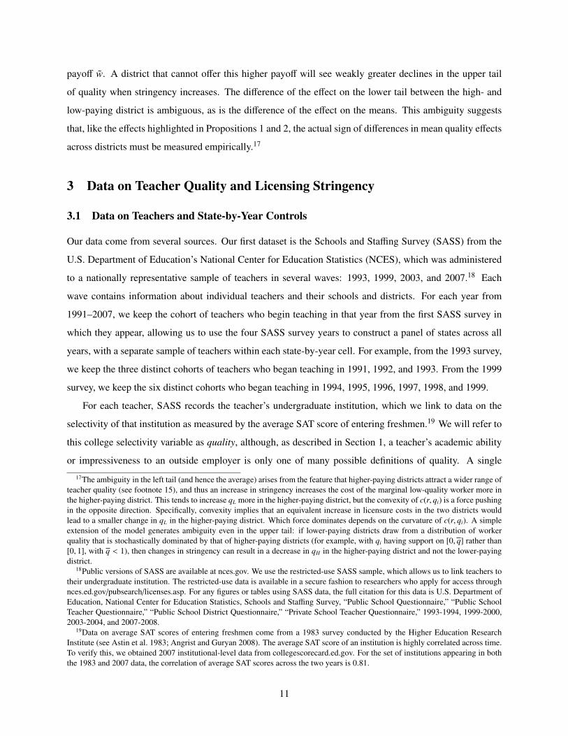
In Section 5 we present the main results. In contrast to most previous studies of occupational licensing

(for teachers or other occupations), our data includes variation in stringency within states over time, allowing

us to control for state and year effects in two-way fixed effects regressions. We find robust positive effects

on the left tail of the quality distribution. The effects are driven by secondary-school teachers, with no

detectable impact on the quality distribution of elementary school teachers.

As highlighted above, we rely on the assumption that, within a given state, changes in licensing strin-

gency are exogenous. It is not possible to rule out all potential violations of this assumption, but we provide a

number of empirical tests that reveal several robust findings. These tests include controlling for state-specific

trends or controlling for changes over time in other educational policies, local labor markets, political and

teacher union environments, and student and school characteristics. In all specifications, we consistently

find a positive and significant effect of licensing stringency on the left tail of the teacher quality distribution

for secondary school teachers. The results are not driven by any single state; the effects are similar with any

state removed from the analysis.

Our main results exploit cases where states increase stringency or decrease stringency (and, in some

cases, states who do both at different times). In Section 5.3, we analyze separately these increases vs.

decreases. Again, we find a robust effect on the left tail: increasing stringency raises the left tail and

decreasing stringency lowers it. Among states that increase stringency, we also detect a significant positive

effect on average quality, but the magnitude is smaller than the left-tail effect. We then use these samples

in an event study design with staggered adoption proposed recently by de Chaisemartin and d’Haultfoeuille

(2020). We find no significant pre-trends and a significant effect of these policy changes on the average and

the left tail in some periods after the policy.

Motivated by the possibility of disparate impacts (e.g., Boyd et al. 2007), we ask whether high-poverty

and high-minority districts show evidence of losing more high-quality teachers in response to increased

3

licensing stringency. We define these vulnerable school districts as those with a high share of minority stu-

dents or a high share of low-income students (who qualify for free lunch). Such districts may struggle to

attract teachers, both on salary and non-salary dimensions (e.g., Prince 2003). We do not find strong evi-

dence of disparate effects: while our confidence intervals do not rule out the possibility that high-minority

or high-poverty districts are negatively affected by increased stringency, the effects are statistically indistin-

guishable from zero. We also find that increased licensing stringency does not negatively affect the diversity

of teacher supply: the fractions of black, Hispanic, Asian, or non-white teachers do not decrease.

Our primary results focus on licensing stringency as measured by academic coursework requirements.

We demonstrate that other dimensions of licensing requirements, such as teacher testing, pedagogy require-

ments, other training requirements, or background checks, are not strongly correlated with our primary

measure of stringency, and factors that do capture these other licensing dimensions do not have robust and

significant effects on the teacher quality distribution. Our results suggest that, if weeding out less aca-

demically qualified candidates from the teaching profession is the desired policy outcome, stricter academic

coursework requirements are an effective instrument.

Our work is related to the empirical literature studying teacher certification. Berger and Toma (1994)

find that a state-level requirement that a teacher have a master’s degree is correlated with lower student test

scores. Goldhaber and Brewer (2000) find that certification exams and field experience requirements have

no significant correlation with average student test scores. Hanushek and Pace (1995) show that requiring

a certification exam reduces the likelihood that a college student becomes a teacher.6 These studies rely on

cross-state variation in licensing requirements. To our knowledge, the only studies to exploit panel variation

in licensing requirements are Angrist and Guryan (2004, 2008). The authors focus on two specific licensing

requirements—basic skills exams and subject matter exams—and exploit variation in these two requirements

in four years (1987, 1990, 1993, and 1999). The authors find no significant effect of these certification test

requirements on the average of the quality distribution (where, as in our study, quality is a teacher’s college

selectivity). While we focus on a larger panel (17 years) and a broader set of teacher requirements (37 rather

than two), our results are consistent with Angrist and Guryan (2004, 2008) in that we do not find strong

effects on average quality in our main specification.

A key contribution of our study is an analysis of the tails of the teacher quality distribution. The debate

6A separate issue that we do not analyze in this paper is that of alternative certification. The term originally derived from a goalto allow high-quality workers from non-education backgrounds (such as those changing careers) to become teachers without havingto complete the full set of requirements for an education degree. Critics argue that, in practice, alternative certification requirementshave evolved to be similar to traditional education school requirements, packaged under a different name (Walsh and Jacobs 2007).Several studies (e.g., Ballou and Podgursky 2000; Rockoff et al. 2008; Kane et al. 2008; Boyd et al. 2006; Sass 2015) comparestudent outcomes and teacher qualifications among teachers holding a standard certification vs. an alternative certification. In arecent handbook chapter, Goldhaber (2011) argues that, relative to these studies, “far less evidence exists on the impact of licensureon the pool of potential teachers.” Our paper relates to this latter question.

4

about how to improve teacher quality has largely revolved around these tails: stricter licensing requirements

are targeted to eliminate the worst-qualified candidates from becoming teachers—moving the left tail of

the quality distribution. And the primary argument against stricter teacher licensing requirements is that

they drive away high-quality candidates—moving the right tail.7 In this paper, we argue that, in addition to

studying effects on average quality, it is informative to study whether licensing stringency has any detectable

effects on other features of the quality distribution, the tails in particular. One study that offers a theoretical

model in which increased licensing stringency can decrease the right tail of teacher quality, is Wiswall

(2007).8 We are not aware of previous work examining the effect of teacher licensing stringency on the left

tail.

Our paper contributes more broadly to the literature studying teacher quality (e.g., Hanushek 2002;

Hanushek and Rivkin 2006). This literature has been particularly concerned about the low ex-ante quality

(prior to becoming a teacher) of those who select into a teaching career, as measured by teachers’ college

selectivity or other measures of academic ability. The literature has also documented how and why the ex-

ante quality of teachers has been declining over time. This literature includes, for example, Nelson (1985),

Hanushek and Pace (1995), Figlio (1997), Bacolod (2007), Hoxby and Leigh (2004), Cochran-Smith and

Fries (2005), Goldhaber and Walch (2013), Jones and Hartney (2017), and Kraft et al. (2020). Ex-post

measures of teacher quality, such as student test scores, have been shown in recent studies to be positively

related to measures of teachers’ academic ability (Dobbie 2011; Xu et al. 2011; Goldhaber et al. 2017;

Hanushek et al. 2019), although existing work also demonstrates that this relationship does not always hold

(Harris and Sass 2011; Kane et al. 2008).9 Our results do not speak to this relationship but instead focus

directly on the selection of new teachers from the ex-ante quality distribution. This focus allows us to study

effects for all states, whereas other measures of quality, such as teacher value-added estimates, are typically

only available in the context of a single state or district.

In work contemporaneous to ours, Kraft et al. (2020) use panel variation in policies adopted from 2011–

2016 regulating the evaluation of new teachers after they begin teaching. The authors document a related

finding to our results: high-stakes evaluation requirements for existing teachers raise the lower tail of the

distribution of quality (as measured by college selectivity) among new teachers. Bruhn et al. (2020) study

the teacher value-added distribution within Massachusetts and find that higher-performing teachers who

7Hanushek (2002) states, “Teacher certification requirements are generally promoted as ensuring that there is a floor on quality,but if they end up keeping out high-quality teachers who do not want to take the specific required courses, such requirements actmore like a ceiling on quality.” Ballou and Podgursky (1998) also argue this point strongly.

8Wiswall (2007) estimates this model using longitudinal survey data and finds that eliminating licensing costs would result in a2.2 percent increase in average teacher quality, as measured by foregone non-teaching wages.

9No single dimension of teacher quality can paint a full picture of what constitutes quality. For example, recent work argues thateven traditional test-score-based measures of teacher value-added miss important non-cognitive performance impacts of teacherson students (Petek and Pope 2016; Jackson 2018).

5

attrit from charter schools move to traditional public schools, and lower-performing charter teachers exit

teaching entirely. The authors propose a model in which this phenomenon can be rationalized by the cost of

obtaining a teaching license (required for teaching in a traditional public school but not a charter school).

We also contribute to a broader literature on occupational licensing—government-mandated require-

ments for professionals in a given occupation. These requirements affect nearly 30% of the U.S. labor force,

a larger proportion of workers than are in unions or covered by minimum wage laws, and over 1,100 occupa-

tions are licensed in at least one state (Kleiner and Krueger 2010).10 A number of previous studies examine

the relationship between licensing laws and quality in a variety of occupations (Carroll and Gaston 1981;

Maurizi 1980; Kleiner and Kudrle 2000; Kugler and Sauer 2005; Barrios 2019; Hall et al. 2019; Kleiner and

Soltas 2019; Farronato et al. 2020; Rupp and Tan 2020). These studies have generally found non-positive

effects on quality. Anderson et al. (2020) offers a recent exception, finding that licensing laws for midwives

in the early 1900s reduced maternal mortality. Two studies that, like ours, study a continuous quality mea-

sure and document positive effects on the left tail of the distribution, are Ramseyer and Rasmusen (2015)

(studying lawyers) and Bhattacharya et al. (2019) (studying financial advisers).11

Previous studies of occupational licensing have also documented the potential for disparate effects for

low-income or minority groups. Currie and Hotz (2004) and Hotz and Xiao (2011) demonstrate that tighter

educational requirements for child care professionals lead to higher quality for children who receive care, but

also lead to price increases resulting in fewer children being served. Kleiner (2006) finds similar results in

dentistry. Law and Marks (2009) and Blair and Chung (2018) offer evidence that occupational licenses can

serve as a positive signal for minority workers, while Federman et al. (2006) find that licensing requirements

for manicurists disproportionately exclude Vietnamese people and Angrist and Guryan (2008) find that

teacher certification test requirements reduce the fraction of Hispanic teachers. In our results, we find no

disparate impacts of increased teacher licensing stringency on these groups.

10Over the past decade, policymakers from both sides of the political spectrum have been especially interested in research andreform surrounding occupational licensing. See http://blogs.wsj.com/washwire/2015/02/09/in-obamas-budget-an-effort-to-rein-in-occupational-licensing/ and https://www.dol.gov/newsroom/releases/eta/eta20180625. Barrero et al. (2020) argue that occupationallicensing restrictions are one of the primary dimensions of U.S. policy that will determine the speed of the economic recovery fromthe COVID-19 pandemic.

11In this broader literature, teacher licensing has been a major focus. See discussions in Kleiner (2006, 2011). Understandingthe effects of licensing laws may be particularly important in the market for public school teachers, where tenure laws make it morechallenging than in other professions to fire low-quality workers, and hence regulating the gateway for initial employment may bedesirable. A theoretical literature studies occupational licensing in general markets for services (e.g., Leland 1979, Shapiro 1986,Kleiner and Soltas 2019). Results from this theoretical literature do not immediately extend to our setting in that the consumers ofschooling services—parents and students—do not directly hire teachers, and wages for teachers are set by public agencies, not bycompetitive market-clearing forces. Because of these features, our theoretical and empirical results do not necessarily immediatelygeneralize to other occupations.

6

2 A Simple Theoretical Framework

We present a simple theoretical model of licensing stringency and the teacher quality distribution. We

consider a static environment with a finite mass of potential teachers (whom we will refer to as workers)

indexed by i. Each worker i is endowed with a quality index qi, which has finite support; without loss of

generality, we consider the support of qi to be [0, 1] for all i. As in the teacher supply models of Angrist and

Guryan (2008) or Kraft et al. (2020), quality in our model is synonymous with the overall strength of the

worker’s resume or qualifications: qi is i’s expected wage outside of teaching.

Each worker chooses to become a teacher or not. If she does not become a teacher, she receives a payoff

of qi. If she does become a teacher, she receives a payoff of w. Unlike markets for other service providers,

such as plumbers or electricians (e.g., Farronato et al. 2020), wages in the teacher market are set by public

agencies (in many cases, through collective wage bargaining with teacher unions) rather than by competitive

market forces. This results in a rigid salary structure that differentiates pay for teachers only based on years

of teaching experience and, in some cases, the level of college degree attained (bachelor’s vs. master’s).12

Because of this feature, we model each teacher as receiving a uniform salary of w that does not depend

on her quality qi. To become a teacher, worker i must pay a cost ci, representing the cost of receiving a

license and getting a teaching position; we will refer to this simply as the cost of licensure.13 We model this

licensure cost as ci = c(r, qi), where r parameterizes the stringency of licensing requirements.

We will refer to the real line R = (−∞,∞) as the extended support of qi. We assume the following

conditions hold at any qi ∈ R:

Assumption 1. At any r and any qi ∈ R, (i) c(r, qi) is continuous and twice differentiable, (ii) ∂c(r,qi)∂r > 0,

(iii) ∂c(r,qi)∂qi

< 0, and (iv) ∂2c(r,qi)∂q2

i> 0.

Assumption 1 states that increases in stringency increase the licensure cost, the cost of licensure is lower

for high-outside-option (high-quality) teachers, and the cost of licensure is strictly convex in qi.14 Define

f (r, qi) = w − c(r, qi) − qi as the expected gains from becoming a teacher. A worker will become a teacher

if and only if f (r, qi) ≥ 0. The strict convexity of c leads to the strict concavity of f , which implies there are12Podgursky (2006) documents that wages and hiring policies in public schools followed this rigid structure in our sample period;

the Wisconsin reform in flexible wages studied in Biasi (2018) occurred in 2011, after our sample period. In contrast to rigid teacherwages, in general service markets with flexible wages and competitive labor market conditions, stricter licensing policies can leadto higher wages in the licensed profession, at least partially accommodating workers for the cost of licensure, as in the recentstructural model of Kleiner and Soltas (2019), or earlier work by Shapiro (1986).

13This model assumes for simplicity that each worker who pays the cost of licensure is also guaranteed a teaching job. In practice,teachers have to be successful in interviews and performance evaluations to be hired (Strauss et al. 2000). We have examined analternative version of this model in which each worker faces a probability of pi of getting a teaching job (in addition to facing a costof licensure), where pi is decreasing in r and increasing in qi. This probability pi can be embedded within ci, and indeed we findthat the alternative model generates the same features we show here. We choose to focus on the simplest model that delivers thesekey insights.

14The strict convexity assumption can be replaced with weak convexity and the results still hold but the proofs are more involved.

7

at most two real roots of f (r, qi) in the extended support of qi. Below we assume a positive mass of workers

choose to be teachers. This implies that f (r, qi) has two distinct real roots and the interval between the two

roots covers at least part of the support [0,1].

Proposition 1. Suppose Assumption 1 holds and a positive mass of workers choose to be teachers. Then

there exists 0 ≤ qL < qH ≤ 1, such that all workers with qi ∈ [qL, qH] choose to become teachers and the

rest do not. Moreover, qL increases with r (and strictly increases if qL > 0) and qH decreases with r (and

strictly decreases if qH < 1).

All proofs are found in Appendix A. Proposition 1 implies that increases in stringency will weakly raise

the lower tail of the distribution of quality within the set of workers who become teachers. This occurs

because increasing stringency raises the cost of licensure, weeding out some low-quality teachers, who have

relatively higher costs of licensure than do high-quality teachers and whose resulting teacher payoff is lower

than their outside option wages. Increasing stringency also weakly lowers the upper tail of the teacher

quality distribution. This occurs because workers in the upper tail have such high outside option wages that

a small increase in the cost of licensure makes teaching unappealing to the marginal high-quality teachers.

The weak monotonicity feature of Proposition 1 is important and relies on the finite support of qi. It

implies that the model can generate a result where the left tail increases without the right tail decreasing

(and vice versa), or a result where neither tail is affected. Which of these changes occurs depends on where

the marginal teachers come from. The left tail is unaffected by increased stringency if the lower root of

f (r, qi) on the extended support of qi is well below zero, capturing a situation in which there are many

low-quality workers willing to become teachers even if licensing costs were to increase. If this lower root

is close to or above zero, raising licensure costs immediately affects the marginal low-quality teacher. A

similar argument holds for the right tail.15

Figure 1 illustrates the results of Proposition 1 as licensing stringency changes from low (top row) to

high (bottom row). The left panels show the case where increased stringency leaves the lower tail of the

pool unchanged while the upper tail of the pool decreases. The right panels feature the case where increased

stringency leads the lower tail of the pool to increase and the upper tail of the pool does not change. The

middle panels illustrate the intermediate case where the lower tail of the pool increases and the upper tail of

the pool decreases.

The following result demonstrates that it is also possible for these changes in the tails to be completely

off-setting, such that the mean is unaffected:15An immediate corollary of Proposition 1 is that an increase in the teaching wage, all else equal, leads to a weak decrease in the

left tail and weak increase in the right tail—the opposite effects of a stringency increase. Our model explicitly assumes that w doesnot depend on r. Any stringency increase accompanied by a teacher salary increase would bias against an empirical finding thatincreased stringency contracts the quality distribution.

8

Figure 1: The Pool of Teachers, Cost Function: c(r, qi) = αr(1 − qi)2

0.0

0.5

1.0

1.5

0.00 0.25 0.50 0.75 1.00Quality

Non−Teachers Teachers

r = 0.3, w = 0.7, alpha = 1

0.0

0.5

1.0

1.5

0.00 0.25 0.50 0.75 1.00Quality


r = 0.3, w = 0.85, alpha = 2

0.0

0.5

1.0

1.5

0.00 0.25 0.50 0.75 1.00Quality


r = 0.3, w = 1, alpha = 3

0.0

0.5

1.0

1.5

0.00 0.25 0.50 0.75 1.00Quality


r = 0.7, w = 0.7, alpha = 1

0.0

0.5

1.0

1.5

0.00 0.25 0.50 0.75 1.00Quality


r = 0.7, w = 0.85, alpha = 2

0.0

0.5

1.0

1.5

0.00 0.25 0.50 0.75 1.00Quality


r = 0.7, w = 1, alpha = 3

Notes: Figure illustrates how the distribution of teacher quality changes with licensing stringency, as described in Proposition 1. For thisillustration, workers are drawn from a Beta(2, 2) and the cost function is c(r, qi) = αr(1 − qi)2. Each column represents different parameters α andteacher wages w. From top panels to bottom panels, licensing stringency r increases. The mass of workers who become teachers is shaded in darkgray and the mass of workers who do not is shaded in light gray.

Proposition 2. Suppose Assumption 1 holds and a positive mass of workers choose to be teachers. An

increase in stringency can result in changes to the tails of the distribution of teacher quality without neces-

sarily changing its mean.

Figure 2 illustrates Proposition 2. An increase in stringency from the left panel to the right panel results

in an increase in the left tail and an off-setting decrease of the same magnitude in the right tail, leaving the

mean unchanged. This proposition is one possible explanation for the null finding in previous studies fo-

cused on the mean rather than tails of the quality distribution (e.g., Angrist and Guryan 2008), and highlights

effects that would be missed by examining only the average quality. The proof of the proposition considers

a particular cost function and a symmetric quality distribution such that changes in stringency result in sym-

metric changes to the upper and lower bounds, leaving the mean unchanged. This mean-preserving property

does not hold in general; Proposition 2 only states that there exists a possibility of a mean-preserving change.

Whether the mean is left unchanged in practice is an empirical question.

We now consider the possibility of two populations facing the same level of licensing stringency and

9

Figure 2: The Mean-Preserving Possibility, Cost Function: c(r, q) =βr

1 + q

0.0

0.5

1.0

1.5

0.00 0.25 0.50 0.75 1.00Quality


r = 0.52, w = 2, beta = 4

0.0

0.5

1.0

1.5

0.00 0.25 0.50 0.75 1.00Quality


r = 0.55, w = 2, beta = 4

Notes: Figure illustrates Proposition 2, where the mean of teacher quality remains unchanged when licensing stringency increases. For thisillustration, workers are drawn from a Beta(2, 2) and the cost function is c(r, qi) =

βr1+qi

. Stringency r increases from the left panel to the right. Themass of workers who become teachers is shaded in dark gray and the mass of workers who do not is shaded in light gray.

the same licensure cost but having different payoffs for teachers. We will refer to these areas here as school

districts. In practice, school districts within a given state may offer different payoffs for teachers even if the

nominal wage w is the same. For example, some districts may offer more classroom support, more funding

for teacher-led initiatives, or better working conditions in general. We capture these non-wage amenities

here by simply subsuming them into a higher nominal teacher wage in one district. Thus, we assume one

district offers a teacher wage w̃ > w while the other district only offers w.16 Our final result relies on one

additional assumption:

Assumption 2. The cost function c(r, qi) satisfies ∂2c(r,qi)∂qi∂r < 0.

This cross-partial condition implies that increases in stringency raise the licensure cost more for low-

quality workers than for high-quality workers.

Proposition 3. Suppose Assumptions 1 and 2 hold and a positive mass of workers choose to be teachers.

When stringency increases, qH decreases weakly less in a district paying w̃ than in a district paying w < w̃.

The difference in the change in qL between the two districts is ambiguous.

Proposition 3 suggests that the potential negative effects of increasing licensing stringency (i.e., the

driving away of high-quality candidates) will be dampened in a school district that can offer a higher real

16Prince (2003) discusses widespread evidence that teachers view these non-wage dimensions of job appeal as analogous to awage gap. There is evidence that high-poverty districts pay less even in nominal wages (Lankford et al. 2002). We also infor-mally interviewed teachers in the San Francisco Bay Area and found similar gaps between high- and low-poverty districts in bothnon-wage amenities and actual pay. Differentials in nominal wages are ostensibly made smaller through policies geared towardequalizing funding across schools, but even these policies have been criticized as leaving loopholes through which high-poverty-area teachers are still paid less nominally (Long 2011).

10

payoff w̃. A district that cannot offer this higher payoff will see weakly greater declines in the upper tail

of quality when stringency increases. The difference of the effect on the lower tail between the high- and

low-paying district is ambiguous, as is the difference of the effect on the means. This ambiguity suggests

that, like the effects highlighted in Propositions 1 and 2, the actual sign of differences in mean quality effects

across districts must be measured empirically.17

3 Data on Teacher Quality and Licensing Stringency

3.1 Data on Teachers and State-by-Year Controls

Our data come from several sources. Our first dataset is the Schools and Staffing Survey (SASS) from the

U.S. Department of Education’s National Center for Education Statistics (NCES), which was administered

to a nationally representative sample of teachers in several waves: 1993, 1999, 2003, and 2007.18 Each

wave contains information about individual teachers and their schools and districts. For each year from

1991–2007, we keep the cohort of teachers who begin teaching in that year from the first SASS survey in

which they appear, allowing us to use the four SASS survey years to construct a panel of states across all

years, with a separate sample of teachers within each state-by-year cell. For example, from the 1993 survey,

we keep the three distinct cohorts of teachers who began teaching in 1991, 1992, and 1993. From the 1999

survey, we keep the six distinct cohorts who began teaching in 1994, 1995, 1996, 1997, 1998, and 1999.

For each teacher, SASS records the teacher’s undergraduate institution, which we link to data on the

selectivity of that institution as measured by the average SAT score of entering freshmen.19 We will refer to

this college selectivity variable as quality, although, as described in Section 1, a teacher’s academic ability

or impressiveness to an outside employer is only one of many possible definitions of quality. A single

17The ambiguity in the left tail (and hence the average) arises from the feature that higher-paying districts attract a wider range ofteacher quality (see footnote 15), and thus an increase in stringency increases the cost of the marginal low-quality worker more inthe higher-paying district. This tends to increase qL more in the higher-paying district, but the convexity of c(r, qi) is a force pushingin the opposite direction. Specifically, convexity implies that an equivalent increase in licensure costs in the two districts wouldlead to a smaller change in qL in the higher-paying district. Which force dominates depends on the curvature of c(r, qi). A simpleextension of the model generates ambiguity even in the upper tail: if lower-paying districts draw from a distribution of workerquality that is stochastically dominated by that of higher-paying districts (for example, with qi having support on [0, q] rather than[0, 1], with q < 1), then changes in stringency can result in a decrease in qH in the higher-paying district and not the lower-payingdistrict.

18Public versions of SASS are available at nces.gov. We use the restricted-use SASS sample, which allows us to link teachers totheir undergraduate institution. The restricted-use data is available in a secure fashion to researchers who apply for access throughnces.ed.gov/pubsearch/licenses.asp. For any figures or tables using SASS data, the full citation for this data is U.S. Department ofEducation, National Center for Education Statistics, Schools and Staffing Survey, “Public School Questionnaire,” “Public SchoolTeacher Questionnaire,” “Public School District Questionnaire,” “Private School Teacher Questionnaire,” 1993-1994, 1999-2000,2003-2004, and 2007-2008.

19Data on average SAT scores of entering freshmen come from a 1983 survey conducted by the Higher Education ResearchInstitute (see Astin et al. 1983; Angrist and Guryan 2008). The average SAT score of an institution is highly correlated across time.To verify this, we obtained 2007 institutional-level data from collegescorecard.ed.gov. For the set of institutions appearing in boththe 1983 and 2007 data, the correlation of average SAT scores across the two years is 0.81.

11

observation in the SASS data represents a particular teacher who began teaching in a particular year and

state, and we can link this observation to the licensing stringency for that year and state. We treat this

observation as an independent draw from the teacher quality distribution in a given year and state.

We standardize the raw quality measure so it has mean zero and variance one within the sample, meaning

all quality results are reported in units of standard deviations of college selectivity. We then compute several

moments of the quality distribution within each state-by-year cell: the average, the 10th percentile, and

the 90th percentile.20 Descriptive statistics for these quality moments across state-year cells are shown at

the top of panel A in Table 1. The first column of Table 1 demonstrates that the mean quality in a state-

year cell is 0 on average (by construction), the 10th percentile of quality is -1.04 on average, and the 90th

percentile is 1.11 on average. The gap between the 10th and 90th percentiles is 2.15 on average. Columns

2–4 demonstrate that these moments differ widely across state-year cells. The final four columns in Table

1 demonstrate that these statistics are similar for elementary and secondary school teachers, although the

quality distribution is wider for secondary school teachers.

Statistics on the number of teachers per state-year cell are reported at the bottom of panel A, and the

total number of state-year cells is shown at the bottom of Table 1. Our SASS sample consists of 26,280

teachers, and includes only state-year cells with at least six teachers, which yields 857 state-by-year cells

when we consider all teachers, 696 state-by-year cells when we consider only elementary school teachers,

and 815 state-by-year cells when we consider only secondary school teachers.21 Panel A displays a number

of other variables we construct from SASS data, including the fraction of schools in city, suburban, or rural

environments; the average (across districts in a state-year cell) percent of minority (non-white) students and

percent of students qualifying for free lunch; several measures of the median teacher earnings within a state-

year cell (the log of public school teacher earnings, the log of district-level salary for new teachers with a

bachelor’s or master’s degree, and the log of private school teacher earnings); and the fraction of teachers

belonging to the union.22

20These state-by-year moments are computed using SASS sampling weights. We aggregate to a group (state-by-year) levelbecause our policy variation (licensing stringency) exists at the state-by-year level and our empirical analysis in Section 5 relies ongrouped quantile regression. Additionally, aggregating (as well as standardizing the college selectivity measure) allows our analysisto rely on data that we can release to other researchers while satisfying NCES reporting requirements.

21We also limit our sample to teachers from school districts with at least 50 students enrolled. Given that we have 17 years and 51states (for our purposes, Washington, D.C. is also treated as a state), we would have 867 state-by-year cells constructed from 26,320teachers. We restrict our sample to state-by-year cells with at least six teachers to satisfy NCES minimum-cell-size requirements,reducing the number of individual teachers to 26,280, and reducing the number of state-year cells to 857. Note that the raw SASSsample sizes are rounded to the nearest 10 to comply with reporting requirements.

22We adjust all monetary quantities throughout the paper to be in 2007 dollars. One of the earnings variables shown in panel A isthe median log of earnings for private school teachers in a state-by-year cell. This variable comes from separate SASS surveys ofprivate school teachers, available the same years as the SASS public school surveys. This data is more sparse than the public schoolteachers sample, and fewer state-by-year cells constructed from this data meet our minimum cell size requirement of six. We setthis variable to zero for any state-by-year cells without at least six observations and we construct a dummy indicator for these cells,denoted “Pri. teacher earnings exists” in Panel A.

12

Our analysis incorporates a number of other state-by-year-level controls. Descriptive statistics for these

state-by-year controls are shown in panel B of Table 1. We obtain information on total student enrollment,

total government spending on education, and the number of charter schools from the U.S. Department of

Education Common Core of Data (CCD). We use data from the Current Population Survey (CPS) Integrated

Public Use Microdata Series (IPUMS, Flood et al. 2020) to construct the state-by-year average wage for all

workers and for public and private school teachers, as well as the fraction of teachers in the union. We also

obtain data on per-capita income from the census and unemployment rate data from the Bureau of Labor

Statistics. We construct a Bartik measure for labor demand following Goldsmith-Pinkham et al. (2020),

which measures wage growth over time accounting for the industry mix within a state. Data on the political

party in control of state executive and legislative branches, as well as an indicator for whether the governor

is a lame duck, come from Klarner (2013a,b). These party variables are coded on a scale with 1 being

Democratic and 0 being Republican.23 The percent of Democratic votes minus the percent of Republican

votes in the state’s most recent gubernatorial election is constructed using the CQ Press Voting and Elections

database. Section 4 discusses additional education policy variables from panel B and Section 5.4 discusses

the teacher race variables from panel A.

3.2 Data on Stringency of Teacher Licensing

The requirements that teachers need to satisfy prior to initial licensure vary widely across states and time

and can consist of dozens of distinct dimensions. For each year possible, we collected data on 37 major

dimensions of licensing requirements in each state (plus Washington, D.C.) from 1991 through 2007 from

a large number of physical and online data sources; see Appendix G for details. Teacher certification re-

quirements include specific coursework and pedagogical training, certification tests, background checks,

and much more. We codify each dimension using binary indicators for whether a requirement in a given

dimension was in place in a given year and state. In each case, 0 indicates less stringency. For example, the

indicator for Humanities takes a value of 1 for a given state and year if teaching candidates were required

to have taken a humanities course prior to initial licensure in that state and year, and takes on a value of 0

otherwise.

The large dimensionality of these requirements necessitates a dimension-reduction approach in order

to make the analysis of licensing stringency feasible and meaningful. We employ principal factor analysis

(PFA) to perform this step. This method reduces a matrix to latent factors that best explain the variation

in the original matrix. Appendix Figure A6, panel B, displays the eigenvalues for each component from

this factor decomposition. The eigenvalue of the first component is nearly three times that of any other,

23See Appendix G for additional details on the construction of the political party and Bartik variables.

13

Table 1: Descriptive Statistics

All Teachers Elementary SecondaryMean SD Min Max Mean SD Mean SD

A: SASS Data Quality MetricsAverage Quality 0.00 0.49 -1.48 1.28 -0.06 0.52 0.06 0.5210th Percentile Quality -1.04 0.73 -3.18 0.77 -0.98 0.72 -1.02 0.7990th Percentile Quality 1.11 0.63 -0.45 3.72 1.00 0.74 1.17 0.7010th-90th Percentile 2.15 0.79 0.37 5.16 1.97 0.82 2.19 0.91

School and Student CharacteristicsFraction City 0.28 0.15 0.00 1.00 0.28 0.19 0.27 0.17Fraction Suburb 0.50 0.19 0.00 1.00 0.51 0.23 0.49 0.20Fraction Rural 0.22 0.19 0.00 1.00 0.21 0.21 0.23 0.20Avg. Percent Free Lunch 35.14 16.62 0.00 80.67 36.45 17.38 34.15 16.83Avg. Percent Minority 41.44 19.16 0.56 99.96 44.04 20.74 39.36 19.57

Teacher Labor MarketLog Pub. Teacher Earnings 10.60 0.15 10.15 11.01 10.58 0.16 10.63 0.15Log District BA Salary 10.48 0.14 10.04 10.78 10.48 0.14 10.48 0.14Log District MA Salary 10.56 0.14 10.13 10.89 10.57 0.14 10.56 0.14Log Pri. Teacher Earnings 8.21 4.15 0.00 10.82 8.27 4.10 8.24 4.12Pri. Teacher Earnings Exists 0.80 0.40 0.00 1.00 0.80 0.40 0.80 0.40Fraction Teachers in Union 0.71 0.24 0.08 1.00 0.71 0.25 0.71 0.25

Teacher RaceFraction Asian 0.02 0.06 0.00 0.90 0.02 0.06 0.02 0.06Fraction Black 0.09 0.10 0.00 1.00 0.08 0.12 0.10 0.12Fraction Hispanic 0.07 0.09 0.00 0.47 0.08 0.12 0.07 0.09Fraction White 0.88 0.11 0.00 1.00 0.89 0.13 0.87 0.13

Num. Obs. Per State-Year 31 15 6 104 11 6 21 10

B: Other Data Sources School/Student Policies and Characteristics (Common Core Data)Total Student Enrollment (k) 1993.59 1679.00 68.45 6441.56 2051.44 1709.33 2008.30 1674.76Log State Educ. Expenditure 23.25 0.96 20.34 24.95 23.28 0.95 23.27 0.96Log No. Charter Schools 2.95 2.13 0.00 6.69 3.05 2.12 2.97 2.14

Teacher Labor Market (CPS)Log Pub. Teacher Earnings 10.41 0.16 9.78 10.93 10.41 0.16 10.41 0.16Log Pri. Teacher Earnings 10.21 0.33 7.59 11.45 10.20 0.33 10.21 0.33Fraction Teachers in Union 0.09 0.06 0.00 0.29 0.09 0.06 0.09 0.06

Non-Teacher Labor MarketBartik Labor Demand -0.75 0.46 -2.14 -0.36 -0.74 0.45 -0.75 0.46Log Per-capita Income 10.43 0.17 9.87 11.08 10.43 0.17 10.43 0.17Log Earnings, All Workers 17.05 0.16 16.60 17.63 17.05 0.15 17.05 0.16Unemployment Rate (BLS) 5.35 1.29 2.30 11.30 5.35 1.29 5.34 1.28

Other Education PoliciesPost Financial Adequacy Policy 0.34 0.47 0.00 1.00 0.35 0.48 0.34 0.47Log No. Desegregation Orders 1.78 1.39 0.00 4.63 1.82 1.40 1.77 1.38Collective Bargaining Required 0.63 0.48 0.00 1.00 0.61 0.49 0.63 0.48Collective Bargaining Allowed 0.10 0.30 0.00 1.00 0.11 0.31 0.09 0.29

Political ConditionsParty of State Legislature 0.41 0.49 0.00 1.00 0.42 0.49 0.39 0.49Party of Governor 0.55 0.42 0.00 1.00 0.55 0.42 0.54 0.42Governor is Lame Duck 0.27 0.44 0.00 1.00 0.27 0.45 0.26 0.44Democrat-Republican Gov. Vote -3.24 18.71 -58.40 83.60 -3.47 18.56 -3.26 18.57

C: Teacher Licensing Requirements DataStringency -0.03 1.01 -1.93 0.85 -0.03 1.01 -0.03 1.01

Total State-Year Observations 857 696 815

Notes: Table shows summary statistics of the quality metrics and SASS data control variables (panel A), control variables from other sources(panel B), and the licensing stringency measure (panel C).

14

suggesting that the first component explains the lion’s share of the variance in licensing requirements; each

successive factor after the first adds little explanatory power. For this reason, we focus primarily on this first

component as our measure of stringency throughout the paper. We analyze other factors in Section 5.5.24

Summary statistics for this stringency measure are reported in panel C of Table 1. Figure 3 displays the

loading of each of the 37 original licensing requirements in our stringency measure (i.e., the weight each

dimension receives). The figure demonstrates that our stringency measure is most strongly correlated with

course requirements for teachers, including social science, natural science, English, math, and humanities;

it is also positively (but less strongly) correlated with teacher training requirements such as student teaching

or knowledge-of-teaching exams; it is weakly negatively correlated with some dimensions, such as evidence

of employment, oath of allegiance, minimum age, and fee requirements. These correlations are particularly

interesting when put in historical context: Ravitch (2003) and other contemporary sources point out that

teacher certification requirements have been influenced and shaped to some extent by teacher preparation

programs and teacher unions (Winkler et al. 2012), who tend to favor certification policies that promote pro-

fessional educator training through education schools and tend to oppose policies that require standards to

be met outside of education schools, such as academic course requirements or academic subject matter test-

ing (Ravitch 2003).25 In this light, our stringency measure captures some of the most important dimensions

surrounding teacher certification debates.

4 Why Does Stringency Vary Across States and Across Years?

We now explore the variation in our stringency measure across states and across time. Teacher licensing

requirements have changed significantly over time, including some changes long before our sample period.

In the mid-1800s, most states began requiring prospective teachers to pass some sort of test to get a teaching

certificate (Ravitch 2003), and by the early 1900s, many states required teachers to have a high school

education and at least some college (Law and Marks 2009). State requirements became less important after

1915, when education schools (initially referred to as normal schools) evolved into the primary educators

of teachers, and the primary drivers of changes in teacher standards for the next several decades, with the

emphasis in teacher training being pedagogical skill rather than academic subject mastery (Ravitch 2003).

The seminal report “A Nation at Risk” in the early 1980s (Gardner 1983) highlighted a number of de-

ficiencies in U.S. education and sparked a new wave of interest in teacher certification reform. Academic

24Note that omitting these other factors from our main analysis does not lead to any bias as these factors are, by construction,orthogonal to one another. Note also that our stringency measure is, by construction, normalized to have mean 0 and standarddeviation 1 across state-year cells.

25See also the contemporary debates between academics (e.g., Darling-Hammond 1997; Darling-Hammond et al. 2001; Ballouand Podgursky 1998).

15

Figure 3: Loadings of Certification Requirements on Stringency Measure

●●●●●

●●●●●●●●●●●●●●●●●●●

●●●●

●●

●●

●●●●●

−0.22

−0.2

−0.17

−0.15

−0.14

−0.08

−0.08

−0.07

−0.05

−0.04

−0.03

−0.02

−0.01

−0.01

0

0.01

0.04

0.05

0.06

0.07

0.07

0.1

0.11

0.11

0.15

0.16

0.17

0.18

0.27

0.27

0.32

0.72

0.9

0.94

0.96

0.96

0.97

Oath of AllegianceKnowledge of US and/or State Constitution

Screening for Moral CharacterMinimum Age Requirement

Fee RequirementBasic Skill ExamNutrition TrainingU.S. Citizenship

FingerprintingTB Test or Chest X−Ray

Health Drug Alcohol TrainingEvidence of Employment

Must Not Be Professional Educ MajorGeneral Knowledge Exam

State Subject Matter RequirementGeneral Health Certificate

Knowledge of Teaching ExamComputer Education Training

Student Teaching Hour RequirementStudies of Subject Matter

Assessment of Teaching PerformanceBA From Accredited Institution

BA From Regionally Accredited InstitutionState Student Teacher EvaluationMust Be Professional Educ Major

Subject Matter ExamSpecial Education Training

Recommendation (College / Employer)General Education Coursework

Field Experience Before Student TeachingBA From State−Approved Institution

Other G.E. Coursework RequirementHumanities Coursework

Math CourseworkEnglish Coursework

Natural Science CourseworkSocial Science Coursework

−0.25 0.00 0.25 0.50 0.75 1.00

Loadings

Notes: Figure displays the factor loading of each of the 37 licensing requirements used in the Principal Factor Analysis (PFA) on the firstcomponent, or our measure of S tringency. Appendix Figures A4–A5 display these loadings for the second and third PFA components.

research that followed demonstrated that the academic ability of public school teachers was lacking (Vance

and Schlechty 1982; Hanushek and Pace 1995; Strauss et al. 2000; Hoxby and Leigh 2004; Bacolod 2007).

However, the level of interest in reform—and the opinions on how to implement such reform—differed

widely across states and across time in the ensuing decades. Heated debates frequently involved one side

arguing for stricter licensing to improve teacher quality while the opposing side argued for looser require-

ments to achieve the same goal.26

26Speaking before the White House in 2003, Diane Ravitch in the NYU Education School stated, “Our nation faces a dauntingchallenge in making sure that we have a sufficient supply of well-educated, well-prepared teachers for our children. There issurely widespread agreement that good teachers are vital to our future. However, there is not widespread agreement about howwe accomplish this goal. Some propose that we raise standards for entry into the teaching profession, while others suggest thatwe lower unnecessary barriers” (Ravitch 2003). A prime example of these opposing viewpoints is the back-and-forth critiques by

16

This heterogeneity of opinion and ideology led to widely varying policies across states in the 1990s and

2000s, a prime example of federalism, with each state functioning as what Supreme Court Justice Louis

Brandeis referred to as a “laboratory of democracy” to “try novel social and economic experiments without

risk to the rest of the country.”27 Even national changes in education policy over this time frame, such as the

No Child Left Behind Act of 2001 (NCLB), led to state-level experiments, leaving it up to individual states

to decide how—and largely when—to achieve the NCLB requirement that each state’s teachers be “highly

qualified teachers”; the precise definition of highly qualified teachers was also left to individual states to

decide (Kuenzi 2009; Kraft 2018).28 Similar examples of variation in policy direction and intensity across

states and time are found in occupational licensing more broadly (Kleiner 2013; Kleiner and Soltas 2019).29

The heterogeneity in teacher licensing requirements across states and across time is demonstrated in Fig-

ure 4. Each panel shows the evolution of a given state’s stringency measure from 1991–2007, with the year

NCLB passed (2001) marked with the vertical line in each plot as a benchmark. Most states are relatively

constant in their stringency score over time.30 Several states experience large increases in stringency, such

as Kentucky and North Dakota. Other states have large decreases in stringency, such as Arkansas, Florida,

and Georgia. Still, others experience large temporary changes, such as the large temporary dip in stringency

observed in Maryland or Michigan or the temporary increase in stringency observed in Alaska or Arizona.

Florida and North Dakota offer a particularly interesting contrast. Both experienced drastic changes in our

stringency measure surrounding NCLB, but in opposite directions. Neighboring South Dakota, on the other

hand, stayed flat over this time frame, while Florida’s neighbor, Georgia, experienced a similar drop, but

several years before Florida.

education researchers (Darling-Hammond et al. 2001 and others, favoring increased requirements and professionalism of teaching)on one side, and Ballou and Podgursky (1998) and Goldhaber and Brewer (2000) on the other, summarized in Cochran-Smith andFries (2005).

27Brandeis quotes from New State Ice Co. v. Liebmann, 285 U.S. 262 (1932), accessed on October 23, 2020 fromhttps://en.wikipedia.org/wiki/Laboratories of democracy. Tamir (2010) offers a detailed historical analysis of the battle of opinionsover teacher certification policy that took place within New Jersey in the 1980s, which resulted in more state-level power overlicensing requirements (and less power in the hands of university teacher preparation programs) and greater emphasis on academicpreparation rather than pedagogical training.

28NCLB specifies that, at a minimum, a highly qualified teacher (HQT) much have a bachelor’s degree and full state licensure andmust prove that she knows her subject matter. Any other dimension of HQT is left up to states to define (as are the specifics of whatconstitutes state licensure and subject-matter knowledge). This freedom led to states reacting differently even to a federal policychange. Furthermore, even if requirements had been uniform across states, these requirements would likely have had asymmetricimpacts on state policy because of cross-state differences in stringency prior to NCLB. Any effects of NCLB on the teacher qualitydistribution that were indeed uniform across states will be captured by year fixed effects in our empirical model.

29Law and Marks (2009) study historical occupational licensing restrictions (from before 1940) across states for a broad rangeof occupations, including teachers. The authors find that southern states were later adopters in requiring teachers to have a highschool education or some college education. Other than this geographic variation, the authors find no systemic explanation for whysome states adopt stricter licensing requirements before others. The authors argue that historical variation in licensing requirementsacross states is in general quite arbitrary. Kleiner (2013) offers similar evidence. Kleiner and Soltas (2019) similarly argue that,for licensed occupations broadly, “the political sources of variation in licensing policy are often so arcane and arbitrary as to beplausibly as good as random.”

30For example, stringency in Illinois does not change during the early-retirement incentive intervention of the early 1990s studiedin Fitzpatrick and Lovenheim (2014).

17

Figure 4: Licensing Stringency Over Time by State

-2-1

01

-2-1

01

-2-1

01

-2-1

01

-2-1

01

-2-1

01

-2-1

01

1990 1995 2000 2005 1990 1995 2000 2005 1990 1995 2000 2005 1990 1995 2000 2005 1990 1995 2000 2005

1990 1995 2000 2005 1990 1995 2000 2005 1990 1995 2000 2005

AK AL AR AZ CA CO CT DC

DE FL GA HI IA ID IL IN

KS KY LA MA MD ME MI MN

MO MS MT NC ND NE NH NJ

NM NV NY OH OK OR PA RI

SC SD TN TX UT VA VT WA

WI WV WY

Lice

nsin

g St

ringe

ncy

Scor

e

Year

Notes: Figure shows the evolution of each state’s stringency measure from 1991–2007, with the year NCLB passed (2001) marked with thevertical line in each panel.

The changes in stringency shown in Figure 4 naturally reflect changes in individual requirements that are

heavily weighted in our stringency measure. For example, the large decrease in stringency in Arkansas in

2002 consists of a removal of coursework requirements in English, social science, natural science, math, and

general education, as well as the removal of a requirement that teachers be professional education majors and

have some field experience before beginning student teaching. All of these requirements receive a positive

loading in the factor analysis shown in Figure 3.

We searched historical discussions for context on the drivers of the teacher licensing stringency changes

found in Figure 4. Several discussions point to perceived teacher shortages as one motive for states reducing

stringency, and Appendix E offers some evidence consistent with this possibility. However, these shortages

were a widespread problem, not limited to specific states (Cortez 2001), and certainly not restricted to

the states in Figure 4 that reduced stringency. Another potential driver highlighted in education policy

discussions during this period is an explicit concern over low teacher quality, and pre-trends here could

18

invalidate the research design we adopt in Section 5. However, these same policy discussions demonstrate

that states showed no clear agreement on how to improve quality, and thus some reduced stringency while

others increased it, while others kept licensing requirements constant (Ravitch 2003). We present results

from an event study in Section 5.3 that support the exogeneity of licensing stringency changes.

As would any 17-year period in the U.S., the period we study naturally encompasses a number of other

education policy changes in different states. Examples of such changes that have received attention in the

recent literature, and that we are able to explicitly control for in our analysis, are school finance reform, the

phasing out of school desegregation orders, changes in state collective bargaining laws, and the rise of char-

ter schools. Panel B of Table 1 contains the following variables at the state-by-year level that relate to these

policies: an indicator for before and after a state adopts its key school finance reform aimed at guaranteeing

sufficient funding to high-poverty districts, obtained from Lafortune et al. (2018), as well as the level of total

government education expenditure from the CCD; the log of the number of districts with a desegregation

order still in place (plus 1), obtained from Reardon et al. (2012); indicators for whether collective bargain-

ing for teachers is required or allowed but not required, obtained from Valletta and Freeman (1988) and

Frandsen (2016); and the log of the number of charter schools (plus 1) from the CCD. We also performed

a detailed reading of other state-level education policy changes over our time period (such as changes in

high school graduation requirements, minimum school day or year length, class size, compulsory school

age requirements, vouchers, or standardized curriculum); we observed no obvious connection between the

timing of these changes and the timing of the stringency changes captured by our metric.31

Overall, our reading of historical discussions and other education policy changes is that the timing and

magnitude of teacher certification requirement changes are as good as random. We offer additional empirical

evidence consistent with this idea in Appendix D, where we show that states’ levels of stringency are not

systematically related to a number of historical educational, political, union, or labor market conditions. In

our estimation in Section 5, we explicitly control for these conditions as much as possible, and in Section 5.3

we present an event study testing for possible differential trends in teacher quality prior to licensing policy

changes.

31A number of state education policy changes occurred before our sample period, such as the wave of policies in the 1970s and1980s aimed at school finance equalization (Jackson et al. 2016). A number of other policy changes occurred after our sampleperiod, such as major accountability/teacher evaluation regulations (adopted after 2011), Race to the Top grants to states (occurringin 2010–2011), and the adoption of Common Core curriculum standards (2009–2010); see Kraft et al. (2020) for a discussion ofsome of these post-2008 policy changes.

19

5 The Effects of Stringency on the Teacher Quality Distribution

5.1 Two-Way Fixed Effects Results

In this section, we describe our empirical approach for measuring the effects of licensing stringency on the

teacher quality distribution and the results of our analysis. For teacher i who began teaching in year t in

state s, let qist be the college selectivity (as measured by the average SAT score of entering freshmen) of

i’s undergraduate institution, standardized to be in units of standard deviations. Let qst (with no i subscript)

represent a statistic of the distribution of qist within a given state-year combination (s, t). The statistics of

the distribution that will be our primary focus are the mean, the 10th percentile, and the 90th percentile.

Our primary methodology is a two-way fixed effects framework. The regressions we analyze take the

following form:

qst = α + γs + λt + S tringencystδ + W′stθ + εst. (1)

Our parameter of interest in equation (1) is δ, the effect of licensing stringency on quality. For example,

when the outcome variable is the 10th percentile of quality in state s and year t, a positive value of δ

would indicate that an increase in licensing stringency from year t − 1 to year t leads to an increase in the

lower tail of quality. A negative value of δ, when the outcome variable is the 90th percentile of quality,

would imply that an increase in stringency decreases the upper tail.32 The vector Wst includes a variety

of state-by-year controls that vary depending on the specification, as we describe below. State effects γs

capture characteristics that are unchanging over time within a state (e.g., some states may have higher-

quality teachers than others over the entire sample period), while year effects λt capture factors that affect

the whole country in a given year (e.g., any nationwide effects of NCLB legislation in the early 2000s).33

32This model is a special case of the grouped quantile regression estimator (Chetverikov et al. 2016a), an alternative to quantileregression for settings with a group-level treatment and micro data on outcomes within a group. In our paper, a group is a state-by-year cell, the treatment of interest is state-by-year level licensing stringency, and micro data corresponds to individual teacherssurveyed in each cell. This estimator offers a number of benefits over traditional quantile regression, including being computation-ally simple to estimate (via ordinary least squares) even with a large number of fixed effects and being robust to measurement errorin computing quantiles (unlike standard quantile regression; see Chetverikov et al. 2016a for details). Because our minimum cellsize is six, the 10th percentile in the smallest cells is equivalent to the 20th, and the 90th percentile is equivalent to the 80th. Ourresults are unchanged if we instead use state-by-year cells with at least ten observations; see Appendix Table A12. Chetverikovet al. (2016a) derive a mild growth condition on the minimum cell size as the number of cells increases such that this measurementerror can also be ignored when computing standard errors. Chetverikov et al. (2016b) extend the method to clustered standarderrors, which we allow for here.

33By construction, there is one cohort in the data per starting year. For example, teachers who began teaching in 1997 appearin the data as third-year teachers surveyed in the SASS 1999 wave, and λ1997 absorbs the mean of qst for this cohort. In additionto any nationwide 1997 effect, average quality for these teachers may differ not because of experience itself (because our qualitymeasure is a fixed characteristic of a teacher that does not vary with experience) but rather because of teacher exit: higher-qualityteachers may be more likely to get high outside offers early and exit teaching. In our regression analysis, year fixed effects absorbaverage quality differences across cohorts due to this type of teacher attrition. Appendix B describes in detail how teacher attritionmay affect our results, and demonstrates empirically that this does not appear to be a driving force in our findings.

20

In our baseline specification, where Wst is empty, our identifying assumption is that unobserved factors

at the state-by-year level (εst) that are not common to all states or all years do not systematically change

at the same time as licensing stringency. As highlighted in Section 4, changes in stringency in response to

past low quality may violate this assumption. The assumption may also be violated if εst contains a number

of other state-by-year factors, such as local labor market conditions, student and school characteristics,

political preferences within a state, or features of education policy apart from licensing stringency. These

factors would not by themselves be a problem for identification, but if these variables covary with stringency

and are omitted from the regression, our identification assumption would be violated.34

We examine the possibility of such omitted variables by consecutively including in the vector Wst a

number of different controls at the state-by-year level. The results are shown in Table 2. To conserve space,

we only show the estimates of the stringency effect δ; estimates for other parameters are found in Appendix

Tables A7–A9. Each cell in Table 2 corresponds to a different regression, with the controls varying across

columns and the outcome and/or sample (all, elementary school, or secondary school teachers) varying

across rows.35 Before presenting the results, we discuss how the controls differ across columns.

All columns in Table 2 include state and year fixed effects. Column 1 is our baseline specification

without any additional control variables (Wst is empty). Column 2 adds controls for the school and student

characteristics listed in panels A and B of Table 1: the urbanicity of the state’s schools, the fraction of

minority students, the fraction of free-lunch students, total enrollment, state expenditures on education,

and the number of charter schools. Column 3 incorporates controls for teacher labor market conditions

(earnings and union strength controls) from panels A and B of Table 1 that might potentially change at

the same time as licensing stringency or drive changes in licensing stringency.36 Column 4 adds controls

for non-teacher labor market conditions listed in panel B of Table 1, including the Bartik measure, the log

of per-capita income, average wages among all workers, and the unemployment rate. This column also

includes quadratic terms of the unemployment rate for state s in year t and three years of lags, as well as

quadratic terms of the unemployment rate in state s in the corresponding SASS survey year.37 Column 5

34Another consideration is that migration of teachers across state lines could change in response to changes in licensing require-ments; Appendix F demonstrates that this is indeed the case, but that the effects do not appear to drive the changes in the distributionof quality that we document here.

35Throughout the paper, unless otherwise stated, regressions use weights constructed from the sum of individual SASS samplingweights within a state-year cell. All standard errors are clustered at the state level.

36Arguments in Kleiner and Petree (1988) and Kleiner (2011) suggest that these union and salary controls may be important, asincreased stringency may increase a union’s wage bargaining power. Arguments in Cowen and Strunk (2015) similarly suggest thatcollective bargaining policies themselves may be important to control for, which we do in column 5. However, as demonstrated inSection 2, any simultaneous increases in salary and stringency should bias against finding an increase in the left tail and a decreasein the right tail.

37Strauss et al. (2000) offer evidence that these unemployment terms could be important for our analysis, as low-qualifiedworkers may be more likely to opt into teaching especially in times of high unemployment: “In a time of difficult employmentprospects, teaching jobs are among the highest paying and the most coveted in many parts of [Pennsylvania].” Note that theearnings and union controls and school/student characteristics constructed from SASS data (listed in panel A of Table 1) capture

21

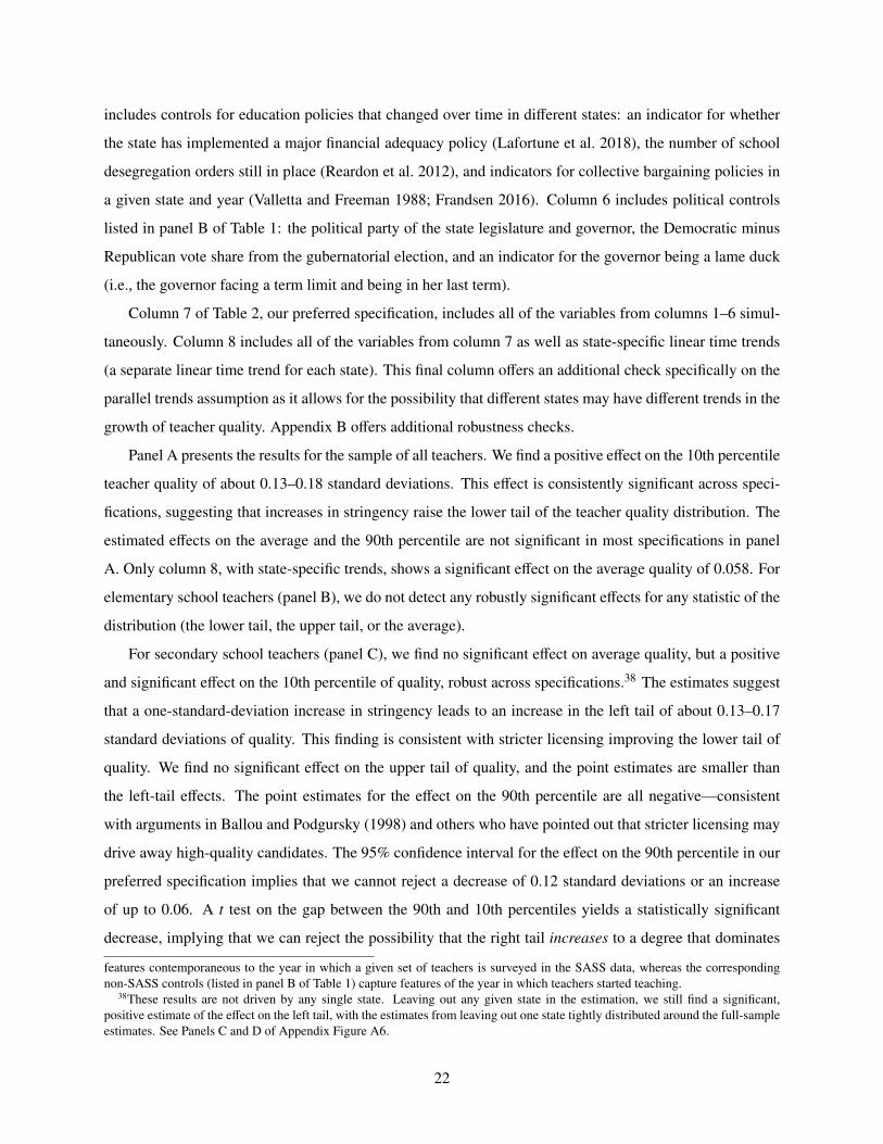
includes controls for education policies that changed over time in different states: an indicator for whether

the state has implemented a major financial adequacy policy (Lafortune et al. 2018), the number of school

desegregation orders still in place (Reardon et al. 2012), and indicators for collective bargaining policies in

a given state and year (Valletta and Freeman 1988; Frandsen 2016). Column 6 includes political controls

listed in panel B of Table 1: the political party of the state legislature and governor, the Democratic minus

Republican vote share from the gubernatorial election, and an indicator for the governor being a lame duck

(i.e., the governor facing a term limit and being in her last term).

Column 7 of Table 2, our preferred specification, includes all of the variables from columns 1–6 simul-

taneously. Column 8 includes all of the variables from column 7 as well as state-specific linear time trends

(a separate linear time trend for each state). This final column offers an additional check specifically on the

parallel trends assumption as it allows for the possibility that different states may have different trends in the

growth of teacher quality. Appendix B offers additional robustness checks.

Panel A presents the results for the sample of all teachers. We find a positive effect on the 10th percentile

teacher quality of about 0.13–0.18 standard deviations. This effect is consistently significant across speci-

fications, suggesting that increases in stringency raise the lower tail of the teacher quality distribution. The

estimated effects on the average and the 90th percentile are not significant in most specifications in panel

A. Only column 8, with state-specific trends, shows a significant effect on the average quality of 0.058. For

elementary school teachers (panel B), we do not detect any robustly significant effects for any statistic of the

distribution (the lower tail, the upper tail, or the average).

For secondary school teachers (panel C), we find no significant effect on average quality, but a positive

and significant effect on the 10th percentile of quality, robust across specifications.38 The estimates suggest

that a one-standard-deviation increase in stringency leads to an increase in the left tail of about 0.13–0.17

standard deviations of quality. This finding is consistent with stricter licensing improving the lower tail of

quality. We find no significant effect on the upper tail of quality, and the point estimates are smaller than

the left-tail effects. The point estimates for the effect on the 90th percentile are all negative—consistent

with arguments in Ballou and Podgursky (1998) and others who have pointed out that stricter licensing may

drive away high-quality candidates. The 95% confidence interval for the effect on the 90th percentile in our

preferred specification implies that we cannot reject a decrease of 0.12 standard deviations or an increase

of up to 0.06. A t test on the gap between the 90th and 10th percentiles yields a statistically significant

decrease, implying that we can reject the possibility that the right tail increases to a degree that dominates

features contemporaneous to the year in which a given set of teachers is surveyed in the SASS data, whereas the correspondingnon-SASS controls (listed in panel B of Table 1) capture features of the year in which teachers started teaching.

38These results are not driven by any single state. Leaving out any given state in the estimation, we still find a significant,positive estimate of the effect on the left tail, with the estimates from leaving out one state tightly distributed around the full-sampleestimates. See Panels C and D of Appendix Figure A6.

22

Table 2: Effects of Licensing Stringency on Teacher Quality Distribution

A. All Teachers (1) (2) (3) (4) (5) (6) (7) (8)Average q: Stringency 0.0181 0.0275 0.0156 0.0175 0.0192 0.00671 0.0163 0.0584∗∗

(0.0257) (0.0308) (0.0250) (0.0254) (0.0242) (0.0287) (0.0283) (0.0248)

10th Percentile q: Stringency 0.155∗∗∗ 0.154∗∗∗ 0.143∗∗∗ 0.131∗∗∗ 0.153∗∗∗ 0.160∗∗∗ 0.141∗∗∗ 0.181∗∗∗

(0.0438) (0.0499) (0.0391) (0.0412) (0.0425) (0.0453) (0.0427) (0.0596)

90th Percentile q: Stringency 0.0241 0.0304 0.0344 0.0509 0.0234 0.0142 0.0413 0.0530(0.0401) (0.0476) (0.0469) (0.0348) (0.0377) (0.0453) (0.0486) (0.0548)

Observations 857 857 857 857 857 857 857 857B. Elementary (1) (2) (3) (4) (5) (6) (7) (8)Average q: Stringency 0.00420 0.0268 -0.00530 -0.00453 0.00590 -0.0131 -0.000124 0.0690

(0.0276) (0.0300) (0.0313) (0.0374) (0.0270) (0.0333) (0.0391) (0.0461)

10th Percentile q: Stringency 0.0835 0.102 0.0574 0.0373 0.0900 0.0817 0.0433 -0.00104(0.0610) (0.0615) (0.0652) (0.0778) (0.0586) (0.0671) (0.0693) (0.0827)

90th Percentile q: Stringency -0.0142 0.0455 -0.0249 -0.00663 -0.0151 -0.0401 0.0295 0.0913(0.0535) (0.0534) (0.0574) (0.0500) (0.0555) (0.0602) (0.0609) (0.0960)

Observations 696 696 696 696 696 696 696 696C. Secondary (1) (2) (3) (4) (5) (6) (7) (8)Average q: Stringency 0.0296 0.0301 0.0356 0.0337∗ 0.0309 0.0228 0.0312 0.0279

(0.0254) (0.0337) (0.0273) (0.0193) (0.0236) (0.0268) (0.0274) (0.0341)

10th Percentile q: Stringency 0.149∗∗∗ 0.143∗∗∗ 0.140∗∗∗ 0.127∗∗∗ 0.147∗∗∗ 0.158∗∗∗ 0.140∗∗∗ 0.167∗∗∗

(0.0325) (0.0419) (0.0326) (0.0364) (0.0289) (0.0342) (0.0383) (0.0523)

90th Percentile q: Stringency -0.0381 -0.0623 -0.00790 -0.0284 -0.0366 -0.0388 -0.0328 -0.00349(0.0739) (0.0781) (0.0734) (0.0450) (0.0711) (0.0726) (0.0482) (0.0680)

Observations 815 815 815 815 815 815 815 815State, Year FE Yes Yes Yes Yes Yes Yes Yes YesSchool Characteristics Yes Yes YesTeacher Market Conditions Yes Yes YesNon-teacher Market Conditions Yes Yes YesEducation Policy Controls Yes Yes YesPolitical Conditions Yes Yes YesState-specific Trends Yes

Notes: Table presents the estimates of equation (1). An observation is a state-year combination. Each cell in the table corresponds to a differentregression and the reported coefficient is the effect of licensing stringency on quality, or δ. Each row represents a different statistic of thedistribution: the mean, the 10th percentile, and the 90th percentile. Each column uses different control variables. All columns include state andyear fixed effects. Column 2-6 adds additional control variables on school/student characteristics, teacher labor market, non-teacher labor market,education policies, and political conditions. Column 7 adds all variables from columns 1–6. Column 8 further includes a separate linear time trendfor each state. Panel A presents the results for all teachers. Panel B restricts to elementary school teachers and Panel C restricts to secondaryschool teachers. Standard errors are clustered at the state level and reported in parentheses. ∗ : p < 0.10, **: p < 0.05, and ***: p < 0.01.

the increase in the left tail.39 Consistent with a large increase in the left tail and a small decrease in the

right tail, we find a small positive (but insignificant) effect on the average. This insignificant effect on the

average quality is consistent with findings of Angrist and Guryan (2008) and with the possibility raised in

39The finding of a large point estimate for the left tail and a smaller for the right is consistent with the range of possibilitiespredicted by Proposition 1. See, for example, the middle column of Figure 1. Note that a very large increase in the left tail canbias us against detecting an decrease in the right tail, as increases primarily affecting lower quantiles can spill over into changesfor higher quantiles. For example, consider a case where quality is initially distributed U[0, 1] and suppose a stringency increasetruncates the support to U[0.46, 0.96], truncating the left tail by far more than the right. In this case, the 90th percentile increasesfrom 0.90 to 0.91 due to the stringency increase, even though the upper bound of the support actually decreases. The t test on thechange in the 90–10 percentile gap, described above, is robust to such changes, and shows that increased stringency indeed leads toa narrowing of the quality distribution.

23

Proposition 2.40 From the 95% confidence interval for the effect on the average, we can reject a negative

effect smaller than -0.02 or a positive effect larger than 0.08.

Several related studies offer interesting benchmarks for the size of our estimated effects. For the sake

of comparison, we focus on the 0.140 increase in the 10th percentile and the 0.0328 decrease in the 90th

percentile (even though the latter is insignificant) from column 7, Table 2, panel C. We define very low-

ranking or high-ranking colleges as those with average SAT scores outside the 10th or 90th percentiles.

These point estimates translate into a 2.1 percentage point (or 21 percent) decrease in the fraction of teachers

coming from very low-ranking colleges and a 0.45 percentage point (or 4.5 percent) decrease in the fraction

coming from very high-ranking colleges.41 Figlio (1997) finds that a 1% increase in average teacher salary

in a school district is associated with a 0.75% increase in the probability that a teacher comes from a selective

college, and a 1% increase in average overall salary in a metropolitan area is associated with a 1.58% increase

in this probability. Bacolod (2007) studies trends from 1971 to 1995 and documents an 11 percentage

point decrease over this period in the fraction of teachers coming from highly-selective colleges and a 16

percentage point increase in the fraction coming from less-selective institutions. Kraft et al. (2020) find

that teacher accountability reforms instituted after 2011 lead to an 8.1 percentage point increase in the

likelihood that a teacher comes from a selective undergraduate institution.42 Relative to these findings, the

magnitude of the effects we find from a one-standard-deviation increase in licensing stringency appears to

be economically meaningful.

We find a significant effect of stringency on the left tail among secondary school teachers and we do not

detect any significant results among elementary school teachers, although the confidence intervals do not rule

out effects of a similar size for the two different teacher types. One possible explanation for this difference

is that some certification requirements may be binding only for secondary school teachers, although the

sources from which we collected the data claim that these requirements apply to both levels of teachers.

An alternative explanation is that, even conditional on college selectivity, secondary school teachers may

have higher-paying outside options than elementary school teachers, such that an equivalent increase in the

licensure cost can affect the career decision of workers on the margin of becoming secondary school teachers

without affecting marginal elementary school teachers.

40Angrist and Guryan (2008) find that a state having a basic skills or subject matter certification test requirement (two of the 37dimensions of licensing requirements we study) does not have a significant effect on the mean of the quality distribution (measuringquality as the average SAT score of teachers’ undergraduate institutions, as in our study) or on the probability that a teacher comesfrom a Carnegie-classified research university or liberal arts college.

41These quantities are approximated by computing 0.1 − F̂(q̂10 − δ̂10) = 0.021 and F̂(q̂90 − δ̂90) − 0.9 = 0.0045, where F̂ denotesthe empirical CDF of individual secondary school teachers’ quality, q̂10 and q̂90 denote the 10th and 90th percentiles of this CDF,and δ̂10 = 0.140 and δ̂90 = −0.0328 are the estimates of the stringency effect on the 10th and 90th percentiles.

42Each of these studies relies on slightly different measures of college selectivity, but these measures tend to be highly correlated,as discussed in Bacolod (2007).

24

5.2 The Full Distribution of Quality

We now examine the effects of increased stringency on the full distribution of quality rather than only the

tails or the average. We evaluate equation (1) with the outcome being the τ percentile, for τ ∈ {10, 20, ..., 90}.

The results are shown in Figure 5. Each point represents δ̂ from a separate regression for each percentile

outcome. For all regressions, we use the preferred specification, with all state-by-year controls included

(corresponding to column 7 of Table 2). 95% confidence intervals (clustered at the state level) for each

percentile are shown with the shaded region.43

Figure 5: Effect of Licensing Stringency on Full Quality Distribution

(A) All Teachers

-.2-.1

0.1

.2

Effe

ct o

f Stri

ngen

cy In

crea

se

0 20 40 60 80 100

Percentile of Quality

(B) Elementary School Teachers

-.2-.1

0.1

.2

Effe

ct o

f Stri

ngen

cy In

crea

se

0 20 40 60 80 100


(C) Secondary School Teachers

-.10

.1.2

Effe

ct o

f Stri

ngen

cy In

crea

se

0 20 40 60 80 100


Notes: Figure presents the effect of increasing licensing stringency on the full distribution of teacher quality, estimated from equation (1). Theoutcomes are the 10th, 20th, ..., 90th percentiles of teacher quality. Panel A uses the full sample of teachers, panel B uses elementary schoolteachers, and panel C uses secondary school teachers. 95% confidence intervals for each percentile are shown with the shaded region, constructedusing seemingly unrelated regression to estimate all quantiles simultaneously and using state-level clustering.

Panel A shows that increased stringency raises the 10th percentile of quality. Point estimates at any

other percentile in panel A—or at any point in the distribution for elementary school teachers in panel B—

are not significantly different from zero. Panel C demonstrates that the increase in the left tail is driven

43These standard errors also take into account cross-quantile correlation in error terms by using seemingly unrelated regression(Zellner 1962) to estimate the effects on all nine quantiles simultaneously.

25

by secondary school teachers, whose quality distribution increases significantly at both the 10th and 20th

percentiles, without any significant effects at other percentiles of the distribution. Other than the 10th and

20th percentiles, the point estimates at nearly every other percentile of the distribution are at or below

zero. The confidence intervals at these other percentiles allow us to reject an effect size that is constant

across quantiles. The evidence points strongly to a narrowing of the quality distribution driven largely by an

increase in the left tail.

5.3 A Closer Look at the Timing of Stringency Changes

Our results in Sections 5.1–5.2 suggest that licensing stringency has its most robust effect on the quality

distribution of secondary school teachers. Here we take a more in-depth look at the precise timing of these

effects. A particular concern for identifying the effect of licensing stringency is the possibility that the

unobserved component εst in equation (1) may be correlated over time within a state, and states may adopt

stricter licensing in response to past low realizations of quality, which would be reflected in a differential

trend in quality in states that change stringency vs. those that do not, prior to the law change. Here we adopt

an event study design to look for such pre-trends.

The state-of-the-art methodology in event study analysis (see Appendix C.1) is most powerful when

treatment is binary and adoption is monotone; that is, when states only change licensing status once over

time, and only in one direction, although the adoption may be staggered across states. To exploit such a

sharp design, we use information in Figure 4 to create a binary treatment variable, classifying each state-

year pair as having either high or low stringency. Specifically, we classify Arkansas, Florida, and Georgia

as beginning with high stringency and changing to low stringency, and we classify Kentucky, Maine, North

Dakota, and Pennsylvania as moving from low to high stringency. A number of other states move in both

directions.44 The remaining states are either always high or always low. We use this classification to create

two subsamples: the high-to-low sample (H2L), consisting of state-year pairs that move only from high

to low stringency, stay always high, or stay always low; and the low-to-high sample (L2H), consisting of

state-year pairs that move only from low to high stringency, stay always low, or stay always high.

Before presenting our event study, in Table 3, we replicate our two-way fixed effects analysis from

columns 1 and 7 of Table 2 using these high-to-low and low-to-high samples. Panel A uses the same

continuous stringency measure as in Table 2, while panel B uses the binary indicator for high stringency.

For average quality, we find a small and insignificant effect in states that changed from high to low strin-

44We classify some states as changing from high-to-low only over a subset of the time period (Alaska after 1994, Arizona after1996, Minnesota before 2002, and Maryland before 1999) and low-to-high over another time frame (Alaska before 1999, Arizonabefore 1999, Minnesota after 1998, and Maryland after 1996). We treat states with minor fluctuations over time as having notchanged stringency; these include Hawaii, Louisiana, Texas, and Connecticut.

26

Table 3: Effect on Secondary School Teacher Distribution in States Increasing vs. Decreasing Stringency

A. Continuous Treatment (1) (2) (3) (4)Average q: Stringency 0.0133 0.00813 0.0770∗∗∗ 0.0951∗∗∗

(0.0312) (0.0337) (0.0266) (0.0318)

10th Percentile q: Stringency 0.151∗∗∗ 0.139∗∗ 0.113∗∗∗ 0.143∗∗∗

(0.0475) (0.0528) (0.0392) (0.0498)

90th Percentile q: Stringency -0.0627 -0.0403 0.0623 0.0243(0.0910) (0.0643) (0.0454) (0.0515)

B. Dummy Treatment (1) (2) (3) (4)Average q: Stringency 0.0304 0.00784 0.138∗∗∗ 0.185∗∗∗

(0.0583) (0.0623) (0.0430) (0.0510)

10th Percentile q: Stringency 0.312∗∗∗ 0.255∗∗ 0.183∗ 0.218∗∗

(0.0916) (0.115) (0.0987) (0.106)

90th Percentile q: Stringency -0.0654 -0.0355 0.136∗ 0.0507(0.198) (0.129) (0.0812) (0.0964)

Observations 727 727 737 737Sample H2L H2L L2H L2HState, Year FE Yes Yes Yes YesAll Controls Yes Yes

Notes: Table displays results from regressing average, 10th percentile, or 90th percentile of secondary school teacher quality in each state-year cellon licensing stringency. Each cell in the table corresponds to a different regression and the reported coefficient is the effect of licensing stringency.Columns 1 and 2 use the sample of states that change stringency from high to low or not at all (H2L) and columns 3 and 4 use the sample of statesthat change stringency from low to high or not at all (L2H). Odd columns include only state and year fixed effects, and even columns include allstate-year controls as in column 7 of Table 2. Panel A uses the same continuous stringency variable as in Table 2, and panel B uses a binaryindicator for high stringency. Standard errors are clustered at the state level. *: p < 0.10, **: p < 0.05, and ***: p < 0.01.

gency (columns 1 and 2), but a significant positive effect in states that changed from low to high stringency

(columns 3 and 4). Both groups of states experienced a significant positive effect on the left tail, and no

significant effect on the 90th percentile. Motivated by these results, we focus on the low-to-high sample for

analyzing the timing of the effect on average quality, and both samples for analyzing the timing of the effect

for the left tail.

Using these binary treatment samples, we perform a staggered-adoption event study following the

method of de Chaisemartin and d’Haultfoeuille (2020) (DCDH). This method aggregates cross-state and

cross-year comparisons in a way that is robust to potential treatment-effect heterogeneity. The DCDH event

study results can be illustrated graphically, as shown in Figure 6. The time 0 estimate corresponds to the

instantaneous change (i.e., the change in the year the treatment occurs) in outcomes for states that change

treatment status vs. those that do not. The time > 0 estimates correspond to the treatment effects of changed

stringency one or more years after the change, and the time < 0 estimates correspond to placebo effects—

those prior to the change in stringency. A significant estimate for a time < 0 effect would suggest a concern-

ing pre-trend, as it would imply that quality was already different in treated states even before the treatment

27

Figure 6: Event Study on Secondary School Teachers

(A) Average Quality, Low-to-High States

-.4-.2

0.2

.4.6

Trea

tmen

t Effe

ct

-3 -2 -1 0 1 2 3Time Since Treatment

(B) 10th Percentile, High-to-Low States

-2-1

01

2Tr

eatm

ent E

ffect


(C) 10th Percentile, Low-to-High States

-1-.5

0.5

1Tr

eatm

ent E

ffect


Notes: Figure shows the results of the staggered-adoption event study following the method proposed in de Chaisemartin and d’Haultfoeuille(2020), with the outcome variable being the average quality (in panel A) or the 10th percentile (in panels B and C) of teacher quality amongsecondary school teachers within a state-year cell. “Treatment” is defined as a change from low to high stringency in panels A and C, and fromhigh to low stringency in panel B. 95% confidence intervals are shown with dashed lines, computed from 200 bootstrap replications, withclustering at the state level.

took place.45

In Figure 6, the results are imprecisely measured, and we do not observe a persistent, discontinuous

jump at time zero characteristic of some event study designs. In contrast, our main regression approach in

Sections 5.1–5.2 offers more power by pooling across post-change years rather than isolating year-by-year

45A traditional event study design consists of replacing S tringencyst in equation (1) with a vector of leads and lags of year-by-year changes in stringency, potentially with some pre-treatment and post-treatment years aggregated into bins. DCDH, as wellas a number of other recent studies (listed in Appendix C.1), demonstrate that such a design is problematic in that it represents aweighted average of average treatment effects (ATEs) across state-year cells with potentially negative weights, which can lead toincorrect estimation and inference if ATEs are heterogeneous across (s, t) pairs. The DCDH methodology does not rely on thesenegative weights, but instead computes the time = 0 effect, for example, by directly comparing outcomes in time t and t − 1 forstates who changed treatment status from t to t− 1. A full description of the DCDH method is quite involved, and we relegate thesedetails to Appendix C.1. There we also discuss that DCDH demonstrate that a standard two-way fixed effects estimator (the mainestimator we rely on in our paper) also relies on potentially negative weights when aggregating ATEs across state-year pairs andthese weights can result in biased estimates in the presence of treatment-effect heterogeneity across state-year pairs. The authorsoffer a number of diagnostics to test whether treatment-effect heterogeneity is indeed problematic for the two-way fixed effectsestimator. We describe the results from these tests in Appendix C.2, which suggest that potential treatment-effect heterogeneitydoes not invalidate our main estimates.

28

effects. However, the event study still offers several insights. First, we detect no significant pre-trends for

either the average quality or left-tail effects, although we do not have sufficient statistical power to claim a

precise zero in each placebo (i.e., pre-treatment) year. Second, we do detect significant effects of the change

in stringency in some years after the treatment occurs: a significant effect on the average and 10th percentile

in year 2 (panels A and C), and a significant effect on the 10th percentile in years 1 and 3 (panel B). This

effect is negative in the high-to-low sample (panel B), as treatment in this sample represents a reduction in

stringency. These results suggest that there is a lag in the effect of changes in licensing stringency. This

is consistent with college students who are prospective teachers changing their majors (in the years before

graduating) in response to changes in licensing requirements. Overall, the results of the event study suggest

that the effects we measure on the quality distribution for secondary school teachers are not driven by any

clear pre-trends in quality; unobservable factors affecting teacher quality do not appear to be changing

differentially in treated vs. untreated states prior to changes in licensing stringency.46

5.4 Effects of Licensing Stringency on Potentially Marginalized Subgroups

We now explore the possibility that changes in licensing stringency may have negative effects on marginal-

ized subgroups of students or teachers, such as high-poverty or high-minority school districts or minority

teachers. Our focus on high-poverty or high-minority districts is motivated by evidence from the existing

literature (e.g., Lankford et al. 2002; Prince 2003; Boyd et al. 2007) that these districts struggle to attract

high-quality teachers.47 Proposition 3 in Section 2 demonstrates that disparate effects are indeed a theoret-

ical possibility: improvements in the quality distribution from changes in licensing stringency may accrue

more to low-poverty districts if these districts can offer higher pay (either through higher nominal pay or

higher non-wage amenities). Section 2 also highlights that it is possible that no differential effect occurs.

Here we investigate this question empirically.

We differentiate school districts on two different dimensions: the percent of students who qualify for

free lunch and the percent of minority students. We construct our data for this analysis by aggregating the

micro data slightly differently from our analysis above. Each observation in the micro-data corresponds to

an individual teacher in the SASS survey, and for each individual teacher, the data records the percent of

46Corresponding event study plots for the specifications that show insignificant effects in Table 3 are found in Appendix FigureA3. These results are also imprecise. For the high-to-low sample effect on the average, we observe placebo effects that are onlymarginally insignificant, underscoring that the effect on the average is less of a robust finding than the effect on the left tail. Wedetect no significant pre-trends for the 90th percentile in either sample, and a significant positive effect two years after the treatmentin the low-to-high treatment sample.

47A teacher quoted in the New York Times in 2000 defended the choice to avoid a job in a high-poverty district: “You have tobe a combination of a social worker and Mother Teresa to work in those schools. Those kids deserve a decent education, but we asteachers deserve a decent work atmosphere. We deserve to be safe. I worked so hard to get my license, I did all this schooling, andthe last thing I heard, America was a country of free choice.” See https://www.nytimes.com/2000/09/01/nyregion/newly-certified-teachers-looking-for-a-job-find-a-paradox.html, cited in Prince (2003).

29

students qualifying for free lunch at that teacher’s school. We classify a micro-data observation as high-

poverty if the percent of students qualifying for free lunch for that micro-data observation is above the

median level of this variable within a given state-by-year cell. We then compute the mean, 10th percentile,

and 90th percentile of quality separately for high-poverty districts and for low-poverty districts within each

state-by-year cell, aggregating the data to the state-by-year-by-poverty-status cell.48 We follow this same

procedure to create a high-minority indicator within each state-by-year cell and aggregate the data to the

state-by-year-by-minority-status cell.

Let HighPovertyst j be an indicator variable denoting whether cell j ∈ {0, 1} in state s and year t contains

high-poverty ( j = 1) or low-poverty ( j = 0) districts. We analyze regressions of the following form:

qst j = α + γs + λt + S tringencystδ + W′stθ + HighPovertyst jψ

+(S tringencyst × HighPovertyst j

)η + εst j, (2)

where qst j here is the statistic of interest of teacher quality within the state-by-year-by-poverty-status cell.

This regression constitutes a grouped quantile regression, as in equation (1), but aggregated to a finer level.

The parameter of interest is η, the parameter on the interaction term, which captures the differential effect

of increased stringency on the quality distribution for high-poverty vs. low-poverty districts. We estimate a

similar version of equation (2) with an indicator HighMinorityst j replacing HighPovertyst j.

Table 4 displays the results from estimating equation (2), where the outcome is either the average quality

(columns 1–3), the 10th percentile of quality (columns 4–6), or the 90th percentile of quality (columns 7–9).

We examine each outcome separately for all teachers, elementary school teachers, and secondary school

teachers. All columns include all state-by-year controls (as in column 7 of Table 2) except that regressions

in panel A do not include the continuous measure of the fraction of students qualifying for free lunch,

and regressions in panel B do not include the continuous measure of the percent of minority students, as

these features are controlled for separately with the binary variables HighPovertyst j and HighMinorityst j.

Appendix Table A10 shows results that are nearly identical using an alternative specification with a full set

of state-by-year fixed effects; this is feasible because in this analysis we have two observations (high-poverty

vs. low-poverty) in many state-by-year cells, unlike in equation (1).

48Relative to our main analysis in Section 5.1, this approach should yield two observations per state-year pair as opposed to one.In practice, the percent of students qualifying for free lunch is constant within some state-year cells, and this leads to only a singleobservation in these cells in our aggregated state-by-year-by-poverty-status data. Another reason we end up with less than doublethe number of observations from our main analysis is that NCES does not allow reporting data from a cell size smaller than 3. Ourminimum cell size at the state-by-year level is 6, and when split into high-poverty vs. low-poverty observations, this cell size shrinksto 3 except in cases where more than half of the observations in a state-by-year cell have the same value for the percent of studentsqualifying for free lunch. In these cases, to comply with reporting requirements, we drop any state-by-year-by-poverty-status cellwith fewer than 3 observations. In the empirical analysis in Appendix Table A10, these cases are absorbed through the inclusion ofstate-by-year fixed effects. This same reasoning applies when we consider high- vs. low-minority observations.

30

Table 4: Heterogeneous Effects of Licensing Stringency on Quality Distribution

Average Quality 10th Percentile 90th PercentileA: High Poverty (1) (2) (3) (4) (5) (6) (7) (8) (9)Stringency 0.0147 -0.00986 0.0416 0.0912∗∗∗ 0.0253 0.181∗∗∗ 0.0289 0.00874 -0.0131

(0.0246) (0.0439) (0.0296) (0.0334) (0.0606) (0.0591) (0.0467) (0.0721) (0.0371)

High Poverty -0.169∗∗∗ -0.171∗∗∗ -0.166∗∗∗ -0.274∗∗∗ -0.280∗∗∗ -0.230∗∗∗ -0.115∗∗ -0.123∗∗∗ -0.0732(0.0399) (0.0456) (0.0434) (0.0713) (0.0860) (0.0608) (0.0561) (0.0389) (0.0864)

Str.*High Poverty -0.000733 0.0228 -0.0141 -0.0869∗ -0.0607 -0.0567 -0.0467 0.0431 -0.0296(0.0262) (0.0395) (0.0339) (0.0475) (0.0539) (0.0618) (0.0356) (0.0457) (0.0520)

Observations 1572 1268 1500 1572 1268 1500 1572 1268 1500

B: High Minority (1) (2) (3) (4) (5) (6) (7) (8) (9)Stringency 0.0310 0.0132 0.0425 0.103∗∗∗ 0.0351 0.0963∗∗∗ -0.00185 0.0165 0.00331

(0.0309) (0.0365) (0.0352) (0.0363) (0.0369) (0.0342) (0.0497) (0.0542) (0.0385)

High Minority -0.0905∗∗ -0.0919 -0.0676 -0.341∗∗∗ -0.317∗∗∗ -0.311∗∗∗ 0.0658∗ 0.0628 0.179∗∗∗

(0.0366) (0.0566) (0.0437) (0.0820) (0.0996) (0.0820) (0.0368) (0.0615) (0.0648)

Str.*High Minority -0.0293 -0.0339 -0.0203 -0.0571 -0.0926 0.0101 0.00940 -0.0375 0.00419(0.0253) (0.0356) (0.0381) (0.0536) (0.0603) (0.0651) (0.0270) (0.0462) (0.0397)

Observations 1704 1373 1620 1704 1373 1620 1704 1373 1620

Sample All Elem Sec All Elem Sec All Elem SecAll Controls Yes Yes Yes Yes Yes Yes Yes Yes Yes

Notes: Table presents heterogeneous effects of licensing stringency on teacher quality, estimated from equation (2). Each observation in theunderlying regressions is a state-by-year-by-poverty-status cell (for panel A) or a state-by-year-by-minority-status cell (for panel B). The outcomeis the mean (in columns 1–3), 10th percentile (in columns 4–6), or 90th percentile (in columns 7–9) of teacher quality. High Poverty and HighMinority are indicators of whether the cell contains high-poverty districts or high-minority districts within a given state and year, and “Str.” standsfor stringency. Each column in each panel represents a separate regression. Columns 1, 4, and 7 show results for all teachers; columns 2, 5, and 8restrict to elementary school teachers; and columns 3, 6, and 9 restrict to secondary school teachers. All regressions include all controls from thepreferred specification (column 7 of Table 2). Standard errors are clustered at the state level and reported in the parentheses. *: p < 0.10, **:p < 0.05, and ***: p < 0.01.

To interpret the coefficient on the interaction term, note that, if the main effect of stringency is positive,

then a negative interaction means that high-poverty or high-minority districts benefit less from increased

stringency. On the other hand, if a main effect of stringency is negative, then a negative interaction implies

that these districts suffer more from increased stringency. The majority of estimated effects for the interaction

terms in Table 4 show negative point estimates, and we cannot reject the possibility of meaningful negative

interaction effects, offering weak evidence consistent with the possibility that vulnerable districts may not

benefit from increased licensing stringency as much as affluent or white-dominated districts (and may even

be harmed). However, none of these potential disparate effects are statistically significant. Importantly, for

the left-tail effect on secondary school teachers (column 6), the total effect of stringency (the combination

of the S tringency main effect and the interaction effect) is positive and statistically significant even for high-

poverty and high-minority districts. The total effect is 0.12 (with a t−statistic of 2.51) for high-poverty

districts and 0.106 (with a t−statistic of 2.09) for high-minority districts, suggesting that even these districts

31

benefit from increased stringency. Together with our main findings in Sections 5.1–5.3, we view the results

in Table 4 as suggesting that increases in licensing stringency lead to a statistically significant improvement

in the left tail of the secondary school teacher quality distribution without leading to any detectable harm to

high-poverty or high-minority districts.49

We conclude this section by examining whether increased licensing stringency has any negative impact

on the diversity of teacher supply as measured by the teacher race. We are motivated by previous findings in

the education literature that certain forms of teacher certification requirements may have negative impacts on

the entry of minority teachers, as well as by mixed findings in the broader occupational licensing literature

showing both negative and positive effects of stricter licensing for minorities (see Section 1). If our key

finding that stricter licensing tends to raise the lower tail of quality is accompanied by decreased teacher

diversity, this benefit may be questionable, especially given that previous studies have demonstrated positive

benefits of minority teachers on students (Gershenson et al. 2016).

Table 5: Effects of Licensing Stringency on Racial Composition of Teachers

(1) (2) (3)Black: Stringency -0.00973 -0.0139 -0.00754

(0.0139) (0.0251) (0.0102)

Asian: Stringency 0.00103 -0.0000994 0.000889(0.00355) (0.00398) (0.00303)

Hispanic: Stringency 0.0154∗∗∗ 0.0129∗ 0.0173∗∗

(0.00480) (0.00744) (0.00805)

Nonwhite: Stringency -0.0111 -0.0180 -0.00742(0.0116) (0.0223) (0.00983)

Observations 857 696 815Sample All Elem SecAll Controls Yes Yes Yes

Notes: Table presents the effects of licensing stringency on teachers’ racial composition, estimated from a two-way fixed effects model similar toequation (1). Each observation is a state-year cell. Each cell in the table corresponds to a different regression and each row represents a differentoutcome: the fraction of black, Asian, Hispanic, and non-white teachers in each state-year cell. The coefficient before S tringency is reported.Column 1 shows results for all teachers, column 2 restricts to elementary school teachers, and column 3 restricts to secondary school teachers. Allregressions include all controls from the preferred specification, as in column 7 of Table 2. Standard errors are clustered at the state level andreported in the parentheses. *: p < 0.10, **: p < 0.05, and ***: p < 0.01.

Table 5 presents the effects of licensing stringency on teachers’ racial composition, estimated from a

two-way fixed effects model similar to equation (1) but with the outcome variable replaced with the fraction

of black, Asian, Hispanic, or non-white teachers in each state-year cell. We find a significant positive impact

of increased stringency on the fraction of Hispanic elementary school teachers. The effect size, about 0.013–

0.017, is economically meaningful given that the average fraction of Hispanic teachers is 0.07 (see Table

1).50 Importantly, we find no significant negative effects of increased stringency on minority participation.49In Appendix E we extend this analysis to examine effects on the quantity of teachers.50This result differs from the negative effect on the fraction of Hispanic teachers documented in Angrist and Guryan (2008),

potentially due to the fact that we focus on different years and on a different measure of licensing stringency.

32

These results, together with those in Table 4, suggest that the increases in licensing requirements captured

by our stringency measure lead to increases in the left tail of teacher quality without significantly negatively

affecting potentially marginalized subgroups of students or teachers.

5.5 Other Dimensions of Licensing Requirements

As highlighted in Section 3, our stringency measure is the first component from the principal factor analy-

sis on all 37 certification dimensions, and places the most weight on requirements of academic coursework

(math, English, social science, natural science, and humanities). This first component explains much more of

the overall variance in licensing requirements than does each of the subsequent components (see Appendix

Figure A6, panel B). Here we examine how the second and third components from the principal factor anal-

ysis relate to the quality distribution. As a rough, partial characterization, the second factor loads heavily on

special training requirements (nutrition, special education, computer education, health/drug/alcohol train-

ing) and performance evaluation, and the third factor loads heavily on certification exams (see Appendix

Figures A4–A5).

Table 6: Effects of Second and Third Principal Factors on Teacher Quality Distribution

(1) (2) (3) (4) (5) (6)Average q: Stringency 0.0259 0.0193 0.0440 -0.00356 0.0239 -0.00508

(0.0221) (0.0360) (0.0313) (0.0216) (0.0389) (0.0286)

10th Percentile q: Stringency 0.0219 -0.0677 0.0680 0.0308 0.0580 0.0495(0.0460) (0.0688) (0.0496) (0.0371) (0.0583) (0.0621)

90th Percentile q: Stringency 0.101∗ 0.0450 0.103∗ -0.00512 -0.0297 0.0305(0.0515) (0.0564) (0.0519) (0.0418) (0.0542) (0.0477)

Observations 857 696 815 857 696 815Principal Factor Factor 2 Factor 2 Factor 2 Factor 3 Factor 3 Factor 3Sample All Elem Sec All Elem SecAll Controls Yes Yes Yes Yes Yes Yes

Notes: Table presents the preferred specification (corresponding to column 7 from Table 2) but with the stringency metric replaced with the secondfactor (in columns 1–3) or third factor (in columns 4–6) from the principal factor analysis. Each cell in the table corresponds to a differentregression and each row to a different outcome. Columns 1 and 4 use all teachers, columns 2 and 5 use elementary school teachers, and columns 3and 6 use secondary school teachers. Standard errors are clustered at the state level and reported in the parentheses. *: p < 0.10, **: p < 0.05, and***: p < 0.01.

In Table 6, we apply our main regression analysis using the second factor (in columns 1–3) or third

factor (in columns 4–6) of licensing stringency. While the confidence intervals are large enough that we

cannot reject substantial effects on the distribution, none of the estimates allow us to reject a zero effect at

the 0.05 level.51 This null result suggests that the interesting and effective variation in teacher certification

51While some effects in Table 6 show statistical significance at the 0.10 level, Appendix Table A11 shows that this marginalsignificance is dependent on whether state-by-year controls are included, unlike the results in Table 2 using the main stringencymeasure.

33

requirements—the variation that truly affects the composition of teachers—consists primarily of the course-

work factors weighted heavily in our primary stringency measure. This result also has important policy

implications: if compliance with these other certification requirements burns real resources (for teachers,

government agencies, and teacher preparation programs) without affecting the distribution of teacher quality,

the effectiveness of these requirements is particularly questionable.

6 Discussion and Conclusion

Our key empirical finding is that stricter licensing requirements lead to a significant increase in the left tail of

teacher quality for secondary school teachers. This finding arises in a two-way (state and year) fixed effects

model, and we demonstrate that this finding is robust to the inclusion of a number of different state-by-year

controls for student and school characteristics, the labor market in and out of the teacher market, political

conditions, and a variety of education-related policies. We also find evidence, in a staggered-adoption event

study, that our results are not driven by differential pre-trends in states adopting stricter licensing. Fur-

thermore, we find that this increase in the left tail is not accompanied by negative effects for marginalized

subgroups of students (high-minority or high-poverty districts) or negative effects on teacher diversity. Inso-

far as policymakers are interested in raising the left tail of the distribution of teachers’ academic ability—and

policy discussions over many decades suggest they are—our findings suggest that increases in teacher li-

censing stringency may be effective.

Our model offers a framework for explaining these empirical findings, as well as for other findings in the

literature and policymakers’ reactions to concerns over teacher quality. In particular, our model demonstrates

that stricter licensing will lead to a weak increase (i.e., an increase or no change) in the left tail of quality and

a weak decrease in the right tail of quality. The model demonstrates moreover that these effects can lead to a

result where the average quality—the focus of some previous empirical studies on teacher certification—can

be relatively unaffected, despite shifts in the tails.

While our study focuses on only one notion of quality—the impressiveness of a teacher’s academic

qualifications—the empirical framework we introduce is amenable to other measures of quality. We have

made our raw certification requirement data publicly available, and one contribution of our analysis is to

highlight the precise natural experiments that have occurred (i.e., those states that have increased or de-

creased their stringency) during this time frame. A natural next step would be to apply our methodology

using different teacher quality metrics, such as parental satisfaction or teacher value-added. However, col-

lecting data on these other dimensions of quality across states and across time would be a costly endeavor,

as these measures are typically only available within a single state.

34

We see our contribution of examining the tails of the quality distribution rather than just the average as

a key idea for the study of teacher certification laws as well as occupational licensing laws more broadly.

These laws are ostensibly intended primarily to weed out low-quality candidates from a given profession (or

prevent low-quality service outcomes). Evidence of regulatory effectiveness is therefore likely to be found

in how these laws affect the left tail of the quality distribution rather than how they affect the average.

References

Anderson, D. M., Brown, R., Charles, K. K., and Rees, D. I. (2020). Occupational licensing and maternalhealth: Evidence from early midwifery laws. Journal of Political Economy, forthcoming.

Angrist, J. and Guryan, J. (2004). Teacher testing, teacher education, and teacher characteristics. AmericanEconomic Review Papers and Proceedings, pages 241–246.

Angrist, J. and Guryan, J. (2008). Does teacher testing raise teacher quality? Evidence from state certifica-tion requirements. Economics of Education Review, 27(5):483–503.

Astin, A., Green, K. C., Korn, W. S., and Maier, M. J. (1983). The American Freshman: National Norms forFall 1983. Cooperative Institutional Research Program of the American Council on Eduaction, HigherEducation Research Institute, Graduate School of Education, UCLA.

Bacolod, M. (2007). Do alternative opportunities matter? The role of female labor markets in the decline ofteacher quality. Review of Economics and Statistics, 89(4):737–751.

Ballou, D. and Podgursky, M. (1998). The case against teacher certification. Public Interest, pages 17–29.

Ballou, D. and Podgursky, M. (2000). Gaining control of professional licensing and advancement. InLoveless, T., editor, Conflicting Missions? Teachers Unions and Educational Reform, pages 69–109. TheBrookings Institution, Washington, DC.

Barrero, J. M., Bloom, N., and Davis, S. J. (2020). COVID-19 is also a reallocation shock. NBER WorkingPaper 27137.

Barrios, J. M. (2019). Occupational licensing and accountant quality: Evidence from the 150-hour rule.Becker Friedman Institute for Research in Economics Working Paper 2018-32.

Ben-Shahar, O. (2017). Teacher certification makes public school education worse, not better. Forbes.Url: https://www.forbes.com/sites/omribenshahar/2017/07/21/teacher-certification-makes-public-school-education-worse-not-better/#33608fae730f. Posted Jul. 17, 2017. Retrieved Aug. 8, 2020.

Berger, M. and Toma, E. (1994). Variation in state education policies and effects on student performance.Journal of Policy Analysis and Management, 13(3):477–491.

Bhattacharya, V., Illanes, G., and Padi, M. (2019). Fiduciary duty and the market for financial advice. NBERWorking Paper 25861.

Biasi, B. (2018). The labor market for teachers under different pay schemes. NBER Working Paper 24813.

35

Blair, P. Q. and Chung, B. W. (2018). Job market signaling through occupational licensing. NBER WorkingPaper 24791.

Boyd, D., Goldhaber, D., Lankford, H., and Wyckoff, J. (2007). The effect of certification and preparationon teacher quality. The Future of Children, pages 45–68.

Boyd, D., Grossman, P., Lankford, H., Loeb, S., and Wyckoff, J. (2006). How changes in entry requirementsalter the teacher workforce and affect student achievement. Education Finance and Policy, 1:176–216.

Bruhn, J. M., Imberman, S. A., and Winters, M. A. (2020). Regulatory arbitrage in teacher hiring andretention: Evidence from Massachusetts charter schools. NBER Working Paper 27607.

Carroll, S. and Gaston, R. (1981). Occupational restrictions and the quality of service received: Someevidence. Southern Economic Journal, pages 959–976.

Chetverikov, D., Larsen, B., and Palmer, C. (2016a). IV quantile regression for group-level treatments, withan application to the distributional effects of trade. Econometrica, 84(2):809–833.

Chetverikov, D., Larsen, B., and Palmer, C. (2016b). Supplement to “IV quantile regression for group-leveltreatments, with an application to the distributional effects of trade”. Econometrica, 84(2):809–833.

Cochran-Smith, M. and Fries, K. (2005). Researching teacher education in changing times: Politics andparadigms. In Cochran-Smith, M. and Zeichner, K. M., editors, Studying Teacher Education: The Reportof the AERA Panel on Research and Teacher Education, pages 69–109.

Cortez, A. (2001). Teacher shortages: Implications for reform and achievement for all students. IDRANewsletter, 28(7):5–7.

Cowen, J. and Strunk, K. O. (2015). How do teachers’ unions influence education policy? What we knowand what we need to learn. Economics of Education Review, 48:208–223.

Currie, J. and Hotz, V. J. (2004). Accidents will happen? Unintended childhood injuries and the effects ofchild care regulations. Journal of Health Economics, 23(1):25–59.

Dale, S. B. and Krueger, A. B. (2002). Estimating the payoff to attending a more selective college: An ap-plication of selection on observables and unobservables. Quarterly Journal of Economics, 117(4):1491–1527.

Darling-Hammond, L. (1997). Doing What Matters Most: Investing in Quality Teaching. National Com-mission on Teaching and America’s Future, Kutztown, PA.

Darling-Hammond, L., Berry, B., and Thoreson, A. (2001). Does teacher certification matter? Evaluatingthe evidence. Educational evaluation and policy analysis, 23(1):57–77.

de Chaisemartin, C. and d’Haultfoeuille, X. (2020). Two-way fixed effects estimators with heterogeneoustreatment effects. American Economic Review, 110(9):2964–2996.

Dobbie, W. (2011). Teacher characteristics and student achievement: Evidence from teach for america.Working paper, Harvard University.

Ellison, K. and Fensterwald, J. (2015). California’s dwindling teacher supply rattling districts’nerves. EdSource. Url: https://edsource.org/2015/californias-dwindling-teacher-supply-rattling-districts-nerves/82805. Posted Jul. 14, 2015. Retrieved Aug. 8, 2020.

36

Farronato, C., Fradkin, A., Larsen, B., and Brynjolfsson, E. (2020). Consumer protection in an online world:An analysis of occupational licensing. NBER Working Paper 26601.

Federman, M., Harrington, D., and Krynski, K. (2006). The impact of state licensing regulations on low-skilled immigrants: The case of Vietnamese manicurists. American Economic Review Papers and Pro-ceedings, 96(2):237–241.

Figlio, D. (1997). Teacher salaries and teacher quality. Economics Letters, 55(2):267–271.

Fitzpatrick, M. D. and Lovenheim, M. F. (2014). Early retirement incentives and student achievement.American Economic Journal: Economic Policy, 6(3):120–54.

Flood, S., King, M., Rodgers, R., Ruggles, S., and Warren, J. R. (2020). Integrated Public Use Mi-crodata Series, Current Population Survey: Version 7.0 [dataset]. Minneapolis, MN: IPUMS, 2020.https://doi.org/10.18128/D030.V7.0.

Frandsen, B. R. (2016). The effects of collective bargaining rights on public employee compensation:Evidence from teachers, firefighters, and police. ILR Review, 69(1):84–112.

Gardner, D. (1983). A Nation At Risk. The National Commission on Excellence in Education, Washington,DC.

Gershenson, S., Holt, S. B., and Papageorge, N. W. (2016). Who believes in me? The effect of student-teacher demographic match on teacher expectations. Economics of Education Review, 52:209–224.

Goldhaber, D. (2011). Licensure: Exploring the value of this gateway to the teacher workforce. In Handbookof the Economics of Education, volume 3, pages 315–339. Elsevier.

Goldhaber, D. and Brewer, D. (2000). Does teacher certification matter? High school teacher certificationstatus and student achievement. Educational Evaluation and Policy Analysis, 22(2):129.

Goldhaber, D., Gratz, T., and Theobald, R. (2017). What’s in a teacher test? Assessing the relationshipbetween teacher licensure test scores and student stem achievement and course-taking. Economics ofEducation Review, 61:112–129.

Goldhaber, D. and Walch, J. (2013). Rhetoric versus reality: Is the academic caliber of the teacher workforcechanging? CEDR Working Paper 2013.

Goldsmith-Pinkham, P., Sorkin, I., and Swift, H. (2020). Bartik instruments: What, when, why, and how.American Economic Review, 110(8):2586–2624.

Hall, J., Hicks, J., Kleiner, M. M., and Solomon, R. (2019). Occupational licensing of uber drivers. Workingpaper, University of Minnesota.

Hanushek, E. and Pace, R. (1995). Who chooses to teach (and why)? Economics of Education Review,14(2):101–117.

Hanushek, E. A. (2002). Teacher quality. In Izumi, L. T. and Evers, W. M., editors, Teacher Quality, pages1–12. Hoover Press, Stanford, CA.

Hanushek, E. A., Piopiunik, M., and Wiederhold, S. (2019). The value of smarter teachers: Internationalevidence on teacher cognitive skills and student performance. Journal of Human Resources, 54(4):857–899.

37

Hanushek, E. A. and Rivkin, S. G. (2006). Teacher quality. Handbook of the Economics of Education,2:1051–1078.

Harris, D. N. and Sass, T. R. (2011). Teacher training, teacher quality and student achievement. Journal ofPublic Economics, 95(7-8):798–812.

Hotz, V. J. and Xiao, M. (2011). The impact of regulations on the supply and quality of care in child caremarkets. American Economic Review, 101(5):1775–1805.

Hoxby, C. M. and Leigh, A. (2004). Pulled away or pushed out? Explaining the decline of teacher aptitudein the united states. American Economic Review, pages 236–240.

Jackson, C. K. (2018). What do test scores miss? The importance of teacher effects on non–test scoreoutcomes. Journal of Political Economy, 126(5):2072–2107.

Jackson, C. K., Johnson, R. C., and Persico, C. (2016). The effects of school spending on educationaland economic outcomes: Evidence from school finance reforms. Quarterly Journal of Economics,131(1):157–218.

Jones, M. and Hartney, M. T. (2017). Show who the money? Teacher sorting patterns and performance payacross US school districts. Public Administration Review, 77(6):919–931.

Kane, T., Rockoff, J., and Staiger, D. (2008). What does certification tell us about teacher effectiveness?Evidence from New York City. Economics of Education Review, 27(6):615–31.

Klarner, C. (2013a). Governors Dataset. Harvard Dataverse, https://doi.org/10.7910/DVN/PQ0Y1N.

Klarner, C. (2013b). State Partisan Balance Data, 1937 - 2011. Harvard Dataverse,https://doi.org/10.7910/DVN/LZHMG3.

Kleiner, M. M. (2006). Licensing Occupations: Ensuring Quality or Restricting Competition? WE UpjohnInstitute, Kalamazoo, MI.

Kleiner, M. M. (2011). Enhancing quality or restricting competition: The case of licensing public schoolteachers. University of Saint Thomas Journal of Law and Public Policy, 5:1.

Kleiner, M. M. (2013). Stages of Occupational Regulation: Analysis of Case Studies. WE Upjohn Institute,Kalamazoo, MI.

Kleiner, M. M. and Krueger, A. B. (2010). The prevalence and effects of occupational licensing. BritishJournal of Industrial Relations, 48(4):676–687.

Kleiner, M. M. and Kudrle, R. T. (2000). Does regulation affect economic outcomes? The case of dentistry.Journal of Law and Economics, 43(2):pp. 547–582.

Kleiner, M. M. and Petree, D. (1988). Unionism and licensing of public school teachers: Impact on wagesand educational output. In Freeman, R. B. and Ichniowski, C., editors, When Public Sector WorkersUnionize. Chigago: University Of Chicago Press.

Kleiner, M. M. and Soltas, E. J. (2019). A welfare analysis of occupational licensing in U.S. states. NBERWorking Paper 26383.

Kraft, M. A. (2018). Federal efforts to improve teacher quality. In Hess, F. M. and McShane, M. Q., editors,Bush-Obama School Reform: Lessons Learned, pages 69–84. Harvard Education Press.

38

Kraft, M. A., Brunner, E. J., Dougherty, S. M., and Schwegman, D. J. (2020). Teacher accountabilityreforms and the supply and quality of new teachers. Journal of Public Economics, 188:104212.

Kuenzi, J. J. (2009). A highly qualified teacher in every classroom: Implementation of the No Child LeftBehind Act and reauthorization issues for the 111th Congress. Congressional Research Service, ReportRL33333.

Kugler, A. and Sauer, R. M. (2005). Doctors without borders? Relicensing requirements and negativeselection in the market for physicians. Journal of Labor Economics, 23(3):437–465.

Lafortune, J., Rothstein, J., and Schanzenbach, D. W. (2018). School finance reform and the distribution ofstudent achievement. American Economic Journal: Applied Economics, 10(2):1–26.

Lankford, H., Loeb, S., and Wyckoff, J. (2002). Teacher sorting and the plight of urban schools: A descrip-tive analysis. Educational Evaluation and Policy Analysis, 24(1):37–62.

Larsen, B. (2015). Occupational licensing and quality: Distributional and heterogeneous effects in theteaching profession. Working Paper, Stanford University.

Law, M. T. and Marks, M. S. (2009). Effects of occupational licensing laws on minorities: Evidence fromthe progressive era. Journal of Law and Economics, 52(2):pp. 351–366.

Leland, H. (1979). Quacks, lemons, and licensing: A theory of minimum quality standards. Journal ofPolitical Economy, pages 1328–1346.

Long, C. (2011). How do we increase teacher quality in low income schools. NEA Today, 24.

Maurizi, A. (1980). The impact of regulation on quality: The case of California contractors. In Rotten-berg, S., editor, Occupational Licensure and Regulation, pages 299–333. American Enterprise Institute,Washington, DC.

Mehta, J. (2013). Teachers: Will we ever learn? New York Times. Url: http://www.nytimes.com/2013/04/13/opinion/teachers-will-we-ever-learn.html. Posted Apr. 12, 2013. Retrieved Apr. 15, 2014.

Nelson, F. H. (1985). New perspectives on the teacher quality debate: Empirical evidence from the nationallongitudinal survey. Journal of Educational Research, 78(3):133–140.

Petek, N. and Pope, N. (2016). The multidimensional impact of teachers on students. Working Paper,University of Maryland.

Podgursky, M. (2006). Teams versus bureaucracies: Personnel policy, wage-setting, and teacher quality intraditional public, charter, and private schools. Education Working Paper Archive.

Prince, C. D. (2003). Higher pay in hard-to-staff schools: The case for financial incentives. ScarecrowPress.

Ramseyer, J. M. and Rasmusen, E. B. (2015). Lowering the bar to raise the bar: Licensing difficulty andattorney quality in Japan. Journal of Japanese Studies, 41(1):113–142.

Ravitch, D. (2003). A brief history of teacher professionalism. Speech presented at the White House Con-ference on Preparing Tomorrow’s Teachers, https://www2.ed.gov/admins/tchrqual/learn/preparing teach-ersconference/ravitch.html. Accessed on October 2, 2020.

39

Reardon, S. F., Grewal, E. T., Kalogrides, D., and Greenberg, E. (2012). Brown fades: The end of court-ordered school desegregation and the resegregation of American public schools. Journal of Policy Anal-ysis and Management, 31(4):876–904.

Rockoff, J., Jacob, B., Kane, T., and Staiger, D. (2008). Can you recognize an effective teacher when yourecruit one? Education Finance and Policy, 6(1):43–74.

Rupp, N. G. and Tan, K. M. (2020). Does occupational licensing improve product quality? Evidence fromthe airline industry. Working Paper, East Carolina University.

Sass, T. R. (2015). Licensure and worker quality: A comparison of alternative routes to teaching. Journalof Law and Economics, 58(1):1–35.

Shapiro, C. (1986). Investment, moral hazard, and occupational licensing. Review of Economic Studies,53(5):843.

Smith, C. (2020). Teacher departures leave schools scrambling for substitutes. AP News. Posted andaccessed Sep. 13, 2020. https://apnews.com/article/indiana-virus-outbreak-archive-911a83b084ec23debadbd92bf559916d.

Strauss, R. P., Bowes, L. R., Marks, M. S., and Plesko, M. R. (2000). Improving teacher preparation andselection: Lessons from the Pennsylvania experience. Economics of Education Review, 19(4):387–415.

Tamir, E. (2010). Capital, power and the struggle over teacher certification. Educational Policy, 24(3):465–499.

Valletta, R. and Freeman, R. B. (1988). The NBER public sector collective bargaining law data set. InFreeman, R. B. and Ichniowski, C., editors, When Public Employees Unionize, pages 399–420. NBERand University of Chicago Press, Chicago.

Vance, V. S. and Schlechty, P. C. (1982). The distribution of academic ability in the teaching force: Policyimplications. The Phi Delta Kappan, 64(1):22–27.

Walsh, K. and Jacobs, S. (2007). Alternative certification isn’t alternative. Thomas B. Fordham Institute.

Winkler, A. M., Scull, J., and Zeehandelaar, D. (2012). How strong are us teacher unions? A state-by-statecomparison. Thomas B. Fordham Institute.

Wiswall, M. (2007). Licensing and occupational sorting in the market for teachers. Working Paper, NYU.

Xu, Z., Hannaway, J., and Taylor, C. (2011). Making a difference? The effects of Teach for America in highschool. Journal of Policy Analysis and Management, 30(3):447–469.

Zellner, A. (1962). An efficient method of estimating seemingly unrelated regressions and tests for aggre-gation bias. Journal of the American statistical Association, 57(298):348–368.

40

A Proofs

Proof of Proposition 1

Proof. Denote the two distinct roots of f (r, qi) as q∗L(r) < q∗H(r), i.e., f (r, q∗L(r)) = f (r, q∗H(r)) = 0. Note that

q∗L and q∗H can differ from qL and qH; the former are roots on the real line and can lie outside of [0, 1], while

the latter are the lowest and highest worker types who choose to become teachers, where worker types have

support on [0, 1]. When a positive mass of workers choose to be teachers, we have q∗H(r) > 0 and q∗L(r) < 1

The strict concavity of f (r, qi), which follows by Assumption 1, implies that f (r, qi) ≥ 0,∀qi ∈ [q∗L(r), q∗H(r)]

and f (r, qi) < 0,∀qi < [q∗L(r), q∗H(r)]. Define qL(r) = max{q∗L(r), 0} and qH(r) = min{q∗H(r), 1}. Then

0 ≤ qL(r) < qH(r) ≤ 1. All workers with qi ∈ [qL(r), qH(r)] ⊂ [q∗L(r), q∗H(r)] choose to become a teacher and

the rest do not, proving the first part of the proposition.

For the second part of the proposition, note that∂ f (r, q∗L(r))

∂qi> 0 and

∂ f (r, q∗H(r))∂qi

< 0. Implicitly

differentiating f (r, q∗L(r)) = 0 with respect to r and using the chain rule yield

∂ f (r, q∗L(r))∂r

+∂ f (r, q∗L(r))

∂qi

∂q∗L(r)∂r

= 0⇒∂q∗L(r)∂r

= −∂ f (r, q∗L(r))

∂r/∂ f (r, q∗L(r))

∂qi> 0.

Similarly, implicitly differentiating f (r, q∗H(r)) = 0 with respect to r and rearranging, we have

∂q∗H(r)∂r

= −∂ f (r, q∗H(r))

∂r/∂ f (r, q∗H(r))

∂qi< 0.

Thus, q∗L strictly increases with r and q∗H strictly decreases with r. When qL > 0, we must have qL = q∗L and

qL strictly increases with r. When qH < 1, we must have qH = q∗H and qH strictly decreases with r.

If instead qL = 0, then q∗L, the lower root, is less than zero, and hence qL will be weakly increasing in r

rather than strictly increasing. And if qH = 1, then q∗H , the upper root, is greater than 1, and hence qH will

be weakly decreasing in r rather than strictly decreasing. �


Proof. For this proof, we only need to show that the mean-preserving property is satisfied for some parametriza-

tion of the model. We consider here c(r, qi) =βr

1 + qifor some finite β > 0, which satisfies Assumption 1.

This cost function is only one example satisfying this property. Other examples can be derived as well, as

long as c(r, qi) is such that f (r, qi) can be written as a quadratic equation q2 + b̃q+ c̃ where b̃ does not depend

on r.

Let β be small enough that some workers choose to become teachers. The two real roots of f (r, qi) are

41

symmetrically distributed aroundw − 1

2:

q∗L =w − 1

2−

√(w + 1)2 − 4βr

2, q∗H =

w − 12

+

√(w + 1)2 − 4βr

2.

Consider some parameterization (w, r, β) such that the model yields a support of quality distribution satisfy-

ing 0 < qL = q∗L < q∗H = qH < 1. Then it follows that qL + qH = w − 1. By Proposition 1, because qL > 0

and qH < 1, a small increase in r will result in a strict increase in qL and a strict decrease in qH , but these

support points will still be symmetrically distributed aroundw − 1

2. If the distribution of qi is symmetric,

the change in r will result in a mean-preserving contraction of the quality distribution. �


Proof. We write q∗H as q∗H(r,w), a function of both the licensing stringency and the wage. Proving the

proposition is equivalent to showing∂2q∗H(r,w)∂r∂w

> 0. Taking the derivative of w−c(r, q∗H(r,w))−q∗H(r,w) = 0

with respect to w yields

1 −∂c(r, q∗H(r,w))

∂qi

∂q∗H(r,w)∂w

−∂q∗H(r,w)

∂w= 0 (3)

⇒∂q∗H(r,w)

∂w= 1/(1 +

∂c(r, q∗H(r,w))∂qi

) = −1/∂ f (r, q∗H(r,w))

∂qi> 0.

Taking the derivative of equation (3) with respect to r yields

∂2c(r, q∗H(r,w))∂qi∂r

+∂2c(r, q∗H(r,w))

∂q2i

∂q∗H(r,w)∂r

∂q∗H(r,w)∂w

+∂c(r, q∗H(r,w))

∂qi

∂2q∗H(r,w)∂w∂r

+∂2q∗H(r,w)∂w∂r

= 0,

Rearranging yields the following expression, with the sign of derivatives shown below each term:

⇒∂2q∗H(r,w)∂w∂r

= −

∂2c(r, q∗H(r,w))

∂qi∂r︸︷︷︸−

+∂2c(r, q∗H(r,w))

∂q2i︸︷︷︸

+

∂q∗H(r,w)∂r︸︷︷︸−

∂q∗H(r,w)

∂w︸︷︷︸+

∂c(r, q∗H(r,w))∂qi

+ 1︸︷︷︸+

> 0.

Thus, qH will decrease weakly more in the low-paying district than in the high-paying district.

To see that the sign of the differential effect on qL is ambiguous, consider first the cost function c(r, qi) =

42

βr1 + qi

, where β > 0. We can solve for q∗L as q∗L(r,w) =w − 1

2−

√(w + 1)2 − 4βr

2. The cross-derivative with

respect to w and r is∂2q∗L(r,w)∂r∂w

= −β(w + 1)((w + 1)2 − 4βr)−3/2 < 0.

In this case, qL will increase weakly more in the low-paying district than in the high-paying district.

Now consider the cost function c(r, qi) = αr(1 − qi)2, where α > 0. When q∗L ∈ [0, 1], we can write it as

follows:52

q∗L(r,w) = 1 −1

2αr−

√1 + 4αr(w − 1)

2αr.

The cross-derivative with respect to w and r is

∂2q∗L(r,w)∂r∂w

= 2α(w − 1)(1 + 4αr(w − 1))−3/2.

Consider w > 1, so∂2q∗L(r,w)∂r∂w

> 0. In this case, qL will increase weakly less in the low-paying district than

in the high-paying district. �

B Teacher Attrition and Estimated Licensing Stringency Effects

As outlined in Section 5, our estimation approach relies on a state-by-year panel from 1991–2007 formed

using four different SASS survey years by grouping together teachers who started teaching in the same

year and same state (and who thus faced the same requirements when initially licensed). For example,

observations for the year 1993 in our state-by-year panel correspond to teachers who are in their first year

of teaching when observed in the 1993 SASS survey; observations for 1999, 2003, and 2007 similarly

contain first-year teachers. Observations for years 1992, 1998, 2002, and 2006 in our state-by-year panel

correspond to teachers observed in a SASS survey in their second year of teaching. Forming our dataset

in this fashion could potentially lead to biased estimates of the treatment effect of licensing stringency if

teachers of different quality levels differ in their likelihood of exiting the profession. If this is the case,

differences in the quality distribution may be driven in part by teacher attrition. We offer a simple theoretical

description of this potential bias here and demonstrate that it does not appear to be an issue in our empirical

analysis.

We consider a comparison of two states for simplicity, which we refer to as states A and B, where A has

a lower level of licensing stringency than B. We examine the quality difference between a cohort of teachers

52Note that this expression and the cross-derivative below only hold for q∗L ∈ [0, 1]. The extended cost function beyond this rangewould be different.

43

in A and B when the cohorts are observed in their first year of teaching vs their second year, at which

point some teachers in each cohort may have exited the profession. Assume teacher quality is uniformly

distributed on [qsL, q

sH] when the cohort of teachers first begins teaching in state s ∈ {A, B}.

Assume the attrition rate (the probability that a teacher exits the profession in a given year) is given by

a for teachers of quality q ≤ φ and by a for teachers with quality q > φ, where 0 ≤ a ≤ a < 1 and where

φ ≥ max{qAL , q

BL} and φ ≤ min{qA

H , qBH}.

53 Thus, teachers with quality below φ exit with a weakly lower

probability, making teacher attrition weakly increasing in teacher quality.54

Let qsτ,y represent the τth percentile of quality among the cohort in state s in year y of teaching. In

year 1 this is given by qsτ,1 ≡ qs

L +τ

100(qs

H − qsL). The τth percentile after a year has passed, qs

τ,2, may

differ from qsτ,1 because of attrition. We first consider this change for the case where τ is a relatively low

percentile of the distribution, such as the 10th percentile, such that max{qAτ,1, q

Bτ,1} ≤ φ. In year 2, a fraction

(1−a)(φ−qsL) + (1−a)(qs

H −φ) of teachers remain in the profession, and the τth percentile of quality among

these second-year teachers in state s is qsτ,2 ≡ qs

L + τ100

(1−a1−a (qs

H − φ) + φ − qsL

).

The difference between the τth percentile among first-year teachers in the two states is given by

∆τ,1 ≡ qBτ,1 − qA

τ,1 = (qBL − qA

L) +τ

100(qB

H − qAH − qB

L + qAL)

The difference between second-year teachers is given by

∆τ,2 ≡ qBτ,2 − qA

τ,2 = (qBL − qA

L) +τ

100

(1 − a1 − a

(qBH − qA

H) − qBL + qA

L

)

The object ∆τ,1 measures the difference in the τth percentile in states A and B solely due to the difference in

licensing stringency faced by the teaching cohort when initially entering, whereas ∆τ,2 measures differences

due both to the direct effect of licensing stringency and to attrition. The difference between ∆τ,1 and ∆τ,2

thus measures a potential bias introduced by comparing teachers observed in their second year rather than

their first, given by

∆τ,2 − ∆τ,1 =τ

100

(a − a1 − a

)(qB

H − qAH) (4)

This expression in (4) implies that the bias will be zero if the attrition rate is constant across percentiles of

quality (i.e., if a = a) or if the upper boundary of the support of the distribution is unchanged by the licensing

53We treat attrition as a function of q as the same in both states.54Lankford et al. (2002) offers some evidence of teacher attrition being higher for teachers with greater earnings potential, and

Wiswall (2007) builds this feature into his model. Other studies also offer evidence suggesting that pursuit of a higher-salary optionis one of the main reasons why teachers leave the profession (Kirby et al. 1999; Prince 2003; Hanushek et al. 2004).

44

policy (i.e., if qBH = qA

H).55 If, instead, a > a, then ∆τ,2 > ∆τ,1 if and only if qBH < qA

H , and ∆τ,2 < ∆τ,1 if and

only if qBH > qA

H . In our case, based on Proposition 1, we expect higher stringency to lead to qBH ≤ qA

H , and

thus ∆τ,2 ≥ ∆τ,1, meaning that using experienced teachers to measure the effect of higher stringency would

potentially overstate the actual effect of the policy on the τth percentile for newly entering teachers (biasing

the estimate toward more positive numbers).

Now consider the effect on a relatively high percentile τ of the distribution, such as the 90th percentile,

such that min{qAτ,2, q

Bτ,2} ≥ φ. For such a τ, the differences in the τth percentile for first-year teachers and

second-year teachers are given by the following:

∆τ,1 ≡ qBτ,1 − qA

τ,1 = (qBH − qA

H) −100 − τ

100(qB

H − qAH − qB

L + qAL)

∆τ,2 ≡ qBτ,2 − qA

τ,2 = (qBH − qA

H) −100 − τ

100

(qB

H − qAH −

1 − a1 − a

(qBL − qA

L))

And the difference between ∆τ,1 and ∆τ,2 is given by

∆τ,2 − ∆τ,1 =100 − τ

100

(a − a1 − a

)(qB

L − qAL) (5)

In (5), the bias will be zero if the attrition rate is constant across percentiles or if the left boundary of the

support is unaffected by the policy change (i.e., if qBL = qA

L). If, instead, a > a, we have ∆τ,2 > ∆τ,1 if and only

if qBL > qA

L , and ∆τ,2 < ∆τ,1 if and only if qBL < qA

L . By Proposition 1, we expect higher stringency to lead to

qBL ≥ qA

L , and thus ∆τ,2 ≥ ∆τ,1, meaning again a potential bias toward more positive numbers. Thus, for upper

percentiles, where Proposition 1 suggests that higher stringency would result in a drop in quality, estimation

using experienced cohorts may understate the quality decrease. These arguments extend immediately to

other cohorts beyond first- and second-year teachers: the more years a cohort has been teaching, the more

biased an estimated effect can be toward positive numbers.

Our empirical analysis in the body of the paper entails some experienced-cohort comparisons such as

those described above. These comparisons do not introduce bias if the attrition rate is relatively constant

across the quality distribution. We now examine this empirically by modifying equation (1) to include

an interaction of S tringency with the number of years a teacher cohort has been teaching when observed

in a SASS survey. The results are shown in Table A1. The specifications in panel A interact stringency

with a linear trend denoting the number of years teaching for a given cohort, and the results in panel B

interact stringency with dummy variables for the number of years teaching. The columns are as in Table 4,

55By extension, this bias will be small if the attrition rate does not differ much across the quality distribution (i.e., a is close to a)or if the upper boundary of the support of the distribution does not change much under the policy (i.e., qB

H is close to qAH).

45

Table A1: Effects of Stringency on Quality Distribution by Cohort Years Teaching

Average Quality 10th Percentile 90th PercentileA: Linear (1) (2) (3) (4) (5) (6) (7) (8) (9)Stringency -0.0155 -0.0617∗ 0.0300 0.170∗∗∗ -0.00855 0.183∗∗∗ -0.0246 -0.0411 -0.0316

(0.0259) (0.0314) (0.0287) (0.0439) (0.0718) (0.0594) (0.0547) (0.0696) (0.0758)

Str.*Years Teaching 0.0135∗ 0.0263∗∗∗ -0.000161 -0.00617 0.0368∗ -0.0143 0.0196 0.0107 -0.00267(0.00752) (0.00847) (0.00938) (0.0166) (0.0193) (0.0178) (0.0158) (0.0181) (0.0187)

B: Dummies (1) (2) (3) (4) (5) (6) (7) (8) (9)Stringency -0.00242 -0.0344 0.0222 0.165∗∗∗ 0.0310 0.126∗ 0.00904 -0.0281 -0.0287

(0.0285) (0.0351) (0.0252) (0.0356) (0.0851) (0.0738) (0.0560) (0.0881) (0.0722)

Str.*(Years Teach == 2) 0.0260 0.0258 0.0362 0.0444 0.0429 0.127 0.000220 0.0175 -0.0229(0.0295) (0.0430) (0.0294) (0.0498) (0.0796) (0.0991) (0.0612) (0.130) (0.0601)

Str.*(Years Teach == 3) 0.00675 0.0339 -0.00831 -0.0908 0.0351 -0.0174 -0.00338 -0.0319 0.0146(0.0301) (0.0321) (0.0356) (0.0655) (0.0490) (0.101) (0.0579) (0.0859) (0.0519)

Str.*(Years Teach == 4) 0.0544 0.106∗∗ 0.00232 -0.00175 0.149 -0.0115 0.0672 0.0839 -0.0383(0.0397) (0.0448) (0.0414) (0.0755) (0.104) (0.0890) (0.0734) (0.0926) (0.0951)

Str.*(Years Teach ≥ 5) 0.0532∗∗ 0.0871∗∗∗ 0.0122 0.00246 0.113 -0.0148 0.0735 0.0291 -0.0149(0.0249) (0.0305) (0.0367) (0.0645) (0.0743) (0.0685) (0.0733) (0.101) (0.0735)

Observations 857 696 815 857 696 815 857 696 815Sample All Elem Sec All Elem Sec All Elem SecAll Controls Yes Yes Yes Yes Yes Yes Yes Yes Yes

Notes: Table presents heterogeneous effects of licensing stringency on the teacher quality interacted with the number of years a teacher cohort hasbeen teaching when observed in SASS data. This is estimated by modifying equation (1) to include a linear interaction with the number of years acohort has been teaching in panel A, and with dummies for the number of years teaching in panel B. “Str.” stands for stringency. Each column ineach panel corresponds to a separate regression. The outcome is the mean (in columns 1–3), 10th percentile (in columns 4–6), or 90th percentile(in columns 7–9) of teacher quality within the cell. Columns 1, 4, and 7 show results for all teachers; columns 2, 5, and 8 restrict to elementaryschool teachers; and columns 3, 6, and 9 restrict to secondary school teachers. All regressions include all state-by-year controls, as in column 7 ofTable 2. Standard errors are clustered at the state level and reported in the parentheses. *: p < 0.10, **: p < 0.05, and ***: p < 0.01.

with columns 1–3 showing effects on average quality, columns 4–6 showing effects on the 10th percentile,

and columns 7–9 showing effects on the 90th percentile. For each outcome, we display the results for all

teachers, elementary school teachers, and secondary school teachers separately. All regressions include all

state-by-year controls from our preferred specification (column 7 of Table 2).56

In both panels, we do not observe any significant differences across cohorts for the effects of stringency

on the secondary school teacher quality distribution (columns 3, 6, and 9). We cannot rule out the possibility

that the effect of stringency on the left tail for secondary school teachers when measured using second-year

teachers is twice as large as that of first-year teachers (the main effect in panel B, column 6 is 0.126, and the

coefficient on the interaction of stringency with the second-year teacher cohort is 0.127). However, the point

estimates for the other interaction terms in column 6 of panel B are negative, as is the interaction term in

column 6 of panel A, and the confidence intervals do not rule out the possibility that the effects are the same

56Note that panel A does not include a main effect for the linear trend for the number of years teaching and panel B does notinclude a main effect for the indicators of the number of years teaching, as year fixed effects absorb these main effects in both cases.In panel B, the omitted years-teaching category dummy is that of first-year teachers.

46

across cohorts. We also find that the estimated coefficient on S tringency for the left tail of the secondary

school teacher distribution is similar to our primary results in Table 2. We therefore do not find evidence

that the potential teacher-attrition bias outlined above is driving our primary results. Column 2 of panels A

and B demonstrate that the effect of stringency on average quality for elementary school teachers, on the

other hand, is statistically significantly larger for more experienced cohorts (and column 1 of panel B shows

that this differential spills over into a differential for the all-teachers sample in the most experienced cohort),

consistent with potential teacher-attrition bias. We do not find these results for elementary school teachers

concerning for our main results, as we do not find robust results for elementary school teacher effects in our

analysis in the body of the paper.

Table A2: Effects of Stringency on Quality Distribution, Controlling for State-Specific Cohort Trends

(1) (2) (3)Average q: Stringency 0.00585 0.00150 0.0107

(0.0345) (0.0431) (0.0355)

10th Percentile q: Stringency 0.134∗∗ 0.0750 0.120∗∗∗

(0.0514) (0.0778) (0.0429)

90th Percentile q: Stringency 0.00401 0.0505 -0.0928(0.0552) (0.0733) (0.0556)

Observations 857 696 815Sample All Elem SecAll State-by-Year Controls Yes Yes YesState-Specific Cohort Trends Yes Yes Yes

Notes: Table presents results analogous to column 8 of Table 2 but with state-specific time trends replaced with state-specific cohort trends. Eachcell in the table corresponds to a different regression and the coefficient before S tringency is reported. Column 1 shows results for all teachers,column 2 restricts to elementary school teachers, and column 3 restricts to secondary school teachers. Standard errors are clustered at the statelevel and reported in the parentheses. *: p < 0.10, **: p < 0.05, and ***: p < 0.01.

An issue that is distinct from the discussion above is that the attrition rate as a function of quality may

potentially vary across states. If this is the case, states may have different trends in the τth percentile of qual-

ity solely due to attrition across cohorts. This is not problematic for our empirical approach unless changes

in the quality distribution due to attrition coincide systematically with changes in licensing stringency. The

event study design in Section 5.3 tests for this possibility, as it tests whether pre-trends in quality across

cohorts are different in treated vs. non-treated states. As another test, Table A2 replicates column 8 of Table

2 but controlling for linear state-specific cohort trends (the years teaching of a given cohort), rather than a

state-specific time trend across all years 1991–2007 as in Table 2. We find similar results to those in Table

2, consistent with cross-state variation in attrition rates not being the driver of our findings.

47

C Technical Details of de Chaisemartin and d’Haultfoeuille (2020)

A number of recent studies have demonstrated that a traditional event study—i.e., replacing S tringencyst in

equation (1) with a vector of leads and lags of year-by-year changes in stringency, potentially with some pre-

treatment and post-treatment years aggregated into bins—is problematic in two-way fixed effects settings.

These studies include Borusyak and Jaravel (2017), Athey and Imbens (2018), Goodman-Bacon (2018), Sun

and Abraham (2018), Callaway and Sant’Anna (2019), and de Chaisemartin and d’Haultfoeuille (2020). The

key takeaway from this literature is that a traditional event study is a weighted average of average treatment

effects across state-by-year cells, with potential negative weights, which can lead to incorrect estimates

and inference. These studies offer alternative proposals for aggregating treatment effects in ways that do

not suffer from this negative-weight critique and that are robust to heterogeneous treatment effects. Some

of these recent proposals also address possible ways to incorporate state-by-year covariates (e.g, Sun and

Abraham 2018 and de Chaisemartin and d’Haultfoeuille 2020), but these approaches are not yet developed

enough to handle a large number of controls such as we have in our preferred specification. We adopt

the primary event study design proposed by de Chaisemartin and d’Haultfoeuille (2020) (DCDH), which

effectively controls for state and year fixed effects but no other state-by-year controls. In this sense, this is a

pure event study, comparing only the differences in outcomes between states that change treatment vs. those

that do not change in particular pairs of years.

C.1 de Chaisemartin and d’Haultfoeuille (2020) Event Study

We consider here a binary treatment with a staggered adoption design (meaning that, for a given state, the

treatment status only changes monotonically and at most once over time), which is the case in which DCDH

obtain their most powerful results. Following the notation of DCDH, let g ∈ {1, ...,G} denote a group and

t ∈ {1, ...,T } denote time.57 Dg,t is the treatment and Yg,t is the outcome of interest. In our setting, g is

a state, t is year, Dg,t is licensing stringency, and Yg,t is some moment of the quality distribution within a

state-year cell. Let Ng,t denote the number of observations in group g and period t. Let Di,g,t, Yi,g,t(0), and

Yi,g,t(1) denote the treatment status and the potential outcomes without and with treatment of observation i

in group g at period t. Let Yi,g,t = Yi,g,t(Di,g,t) denote the realized outcome. Define Dg,t = 1Ng,t

∑Ng,t

i=1 Di,g,t,

Yg,t(0) = 1Ng,t

∑Ng,t

i=1 Yi,g,t(0), Yg,t(1) = 1Ng,t

∑Ng,t

i=1 Yi,g,t(1), and Yg,t = 1Ng,t

∑Ng,t

i=1 Yi,g,t. We assume the treatment is

homogeneous, so Di,g,t = Dg,t,∀i.

Let NS =∑

(g,t):t≥2Dg,t,Dg,t−1 Ng,t. For t ∈ {2, ...,T } and d, d′ ∈ {0, 1}2, let Nd,d′,t denote the number of

observations with treatment d′ at period t − 1 and treatment d at period t, or Nd,d′,t =∑

g:Dg,t=d,Dg,t−1=d′ Ng,t.

57Note that DCDH use the term group differently from Chetverikov et al. (2016a): in the Chetverikov et al. (2016a) nomenclature,a group is a state-by-year cell, whereas in DCDH a group is a state. For this section we follow the DCDH use of the term.

48

Thus, NS =T∑

t=2(N1,0,t + N0,1,t). Define δS as the average treatment effect of all switching cells, given by

δS = E

1NS

∑(i,g,t):t≥2,Dg,t,Dg,t−1

[Yi,g,t(1) − Yi,g,t(0)

]. Define

DID+,t =∑

g:Dg,t=1,Dg,t−1=0

Ng,t

N1,0,t

(Yg,t − Yg,t−1

)−

∑g:Dg,t=Dg,t−1=0

Ng,t

N0,0,t

(Yg,t − Yg,t−1

),

DID−,t =∑

g:Dg,t=Dg,t−1=1

Ng,t

N1,1,t

(Yg,t − Yg,t−1

)−

∑g:Dg,t=0,Dg,t−1=1

Ng,t

N0,1,t

(Yg,t − Yg,t−1

).

If N1,0,t = 0 or N0,0,t = 0, let DID+,t = 0. If N1,1,t = 0 or N0,1,t = 0, let DID−,t = 0. DCDH propose the

following estimator and demonstrate that it satisfies consistency and asymptotic normality:

DIDM =

T∑t=2

(N1,0,t

NSDID+,t +

N0,1,t

NSDID−,t

).

The t = 0 estimates in Figure 6 in the body of the paper correspond to estimates of DIDM. Given that a

change in a group’s treatment status may affect the outcome for more than one period, the researcher may

be interested in not only the treatment effect at the period when the group receives treatment (t = 0), but

also the lasting effects at later periods (t > 0). The DCDH estimator estimates these dynamic effects through

comparing the changes in outcomes from t − 1 to t + 1 in groups that switch and do not switch treatment

between t − 1 and t.58

Let NdyS =

∑(g,t):2≤t≤T−1Dg,t+1=Dg,t,Dg,t−1 Ng,t. For all t ∈ {2, ...,T − 1} and for all (d, d′, d′′) ∈ {0, 1}3, let

Nd,d′,d′′,t denote the number of observations with treatment d′′ at period t − 1, treatment d′ at period t, and

treatment d at period t + 1, or Nd,d′,d′′,t =∑

g:Dg,t+1=d,Dg,t=d′,Dg,t−1=d′′ Ng,t; thus, NdyS =

T∑t=3

(N1,1,0,t + N0,0,1,t).

Define

DIDdy+,t =

∑g:Dg,t+1=Dg,t=1,Dg,t−1=0

Ng,t

N1,1,0,t

(Yg,t+1 − Yg,t−1

)−

∑g:Dg,t+1=Dg,t=Dg,t−1=0

Ng,t

N0,0,0,t

(Yg,t+1 − Yg,t−1

),

DIDdy−,t =

∑g:Dg,t+1=Dg,t=Dg,t−1=1

Ng,t

N1,1,1,t

(Yg,t+1 − Yg,t−1

)−

∑g:Dg,t+1=Dg,t=0,Dg,t−1=1

Ng,t

N0,0,1,t

(Yg,t+1 − Yg,t−1

).

If N1,1,0,t = 0 or N0,0,0,t = 0, let DIDdy+,t = 0. If N1,1,1,t = 0 or N0,0,1,t = 0, let DIDdy

−,t = 0. The dynamic

58The estimator for these dynamic effects is not explicitly stated in DCDH; we derive it here following the authors’ notation. deChaisemartin and D’Haultfœuille (2020a) offer a similar presentation and further discussion.

49

estimator of the average treatment effect in one period after the switch is defined as

DIDdyM =

T−1∑t=2

N1,1,0,t

NdyS

DIDdy+,t +

N0,0,1,t

NdyS

DIDdy−,t

.The dynamic estimator for other periods can be defined similarly. The t > 0 estimates in Figure 6 in the

body of the paper correspond to these dynamic effect estimates.

Similar to the standard two-way fixed effects model, the consistency of DIDM relies on the common-

trends assumption, as it uses groups whose treatment is stable across two periods to infer the trends that

would have affected switchers if their treatment status had not changed. This assumption could fail if

switchers experience different trends than groups whose treatment is stable. To test the validity of the

common-trends assumption, the authors propose the following placebo estimator that compares the changes

in outcomes from t − 2 to t − 1 in groups that switch treatment and in groups that do not switch treatment

between t− 1 and t, analogous to the pre-period placebo tests in a standard event study analysis, but adapted

to the DIDM estimator.

Let NplS =

∑(g,t):t≥3Dg,t,Dg,t−1=Dg,t−2 Ng,t. For all t ∈ {3, ...,T } and for all (d, d′, d′′) ∈ {0, 1}3, let Nd,d′,d′′,t

denote the number of observations with treatment d′′ at period t−2, treatment d′ at period t−1, and treatment

d at period t, or Nd,d′,d′′,t =∑

g:Dg,t=d,Dg,t−1=d′,Dg,t−2=d′′ Ng,t; thus, NplS =

T∑t=3

(N1,0,0,t + N0,1,1,t). Define

DIDpl+,t =

∑g:Dg,t=1,Dg,t−1=Dg,t−2=0

Ng,t

N1,0,0,t

(Yg,t−1 − Yg,t−2

)−

∑g:Dg,t=Dg,t−1=Dg,t−2=0

Ng,t

N0,0,0,t

(Yg,t−1 − Yg,t−2

),

DIDpl−,t =

∑g:Dg,t=Dg,t−1=Dg,t−2=1

Ng,t

N1,1,1,t

(Yg,t−1 − Yg,t−2

)−

∑g:Dg,t=0,Dg,t−1=Dg,t−2=1

Ng,t

N0,1,1,t

(Yg,t−1 − Yg,t−2

).

If N1,0,0,t = 0 or N0,0,0,t = 0, let DIDpl+,t = 0. If N1,1,1,t = 0 or N0,1,1,t = 0, let DIDpl

−,t = 0. The placebo

estimator for one period before the switch is defined as

DIDplM =

T∑t=3

N1,0,0,t

NplS

DIDpl+,t +

N0,1,1,t

NplS

DIDpl−,t

.The placebo estimator for other periods can be defined similarly. The authors demonstrate that, under

the common-trends assumption (and other conditions detailed in their paper), E(DIDplM) = 0, and thus this

placebo estimator can be used to evaluate the validity of the common-trends assumption. The t < 0 estimates

in Figure 6 in the body of the paper correspond to these placebo effect estimates.

50

C.2 Diagnostic Tests from de Chaisemartin and d’Haultfoeuille (2020)

In the body of the paper, we use a two-way fixed effects estimator as our main approach because it allows

us to increase power by pooling across years following changes in stringency rather than only estimating

a treatment effect at the time of a stringency change, which is what the DIDM (t = 0) estimator captures.

The two-way fixed effects regression (written here with no state-by-year controls, for simplicity) is Yg,t =

α+γg+λt +βf eDg,t +εg,t, where β f e is the coefficient of interest. The first-difference regression is ∆Yg,t = ζt +

β f d∆Dg,t +εg,t, where ∆Yg,t = Yg,t−Yg,t−1, ∆Dg,t = Dg,t−Dg,t−1, and β f d is the coefficient of interest. DCDH

show that ordinary-least-squares estimates of β̂ f e or β̂ f d can be written as a weighted sum of the treatment

effects in each group and time, with some of these weights potentially being negative. If the treatment

effect is constant across groups and time, it can be identified under the standard common-trends assumption.

However, if the treatment effect is heterogeneous across groups or time, both β̂ f e and β̂ f d can potentially

be negative even if all group-time treatment effects are in fact positive, due to these negative weights. The

authors suggest two diagnostic exercises to evaluate whether potential heterogeneity in treatment effects is

indeed problematic in a given application.

The first test compares the two-way fixed effects estimator, β̂ f e, to the first-difference estimator, β̂ f d.

The authors demonstrate that this comparison serves to test whether the weights attached to these estimators

are uncorrelated with the treatment effect in treated cells (testing Assumptions 7 and 8 in DCDH). If β̂ f e

and β̂ f d are not significantly different, treatment-effect heterogeneity may be present without biasing β̂ f e. In

Table A3 we compare the two estimators for our main robust findings from the paper (the left-tail effect for

secondary school teachers). We find that the two estimators do not differ substantially and their confidence

intervals overlap, consistent with treatment-effect heterogeneity not being problematic for our main findings.

Table A3: Two-Way Fixed Effects and First-Difference Estimators for Secondary School Teacher Left Tail

(1) (2) (3) (4)Stringency 0.149∗∗∗ 0.140∗∗∗

(0.0325) (0.0383)

First-Difference of Stringency 0.232 0.266(0.171) (0.189)

Observations 815 750 815 750State, Year FE Yes Yes Yes YesAll State-by-Year Controls Yes Yes

Notes: Table compares the two-way fixed effects estimator and the first difference estimator. The estimates show the effect of licensing stringencyon the left tail of the quality distribution for secondary school teachers. All regressions include state and year fixed effects. Columns 1 and 2include no additional controls. Columns 3 and 4 include all state-by-year controls, as in our preferred specification. Columns 1 and 3 show thefixed effects estimator, corresponding to the specification from columns 1 and 7 of Table 2, Panel C, Row 2. Columns 2 and 4 show thefirst-difference estimator. Standard errors are clustered at the state level and reported in the parentheses. *: p < 0.10, **: p < 0.05, and ***:p < 0.01.

51

The second test quantifies the degree of treatment-effect heterogeneity that would invalidate the esti-

mated treatment effect. The authors define σ f e as the minimal value of the standard deviation of the average

treatment effects across treated cells that is compatible with the true average treatment effect being zero.

This quantity can be calculated as the ratio of the absolute value of β̂ f e divided by the standard deviation of

the weights. We compute this quantity in our preferred specification for the left-tail effect among secondary

school teachers. We find that σ f e is 0.116, suggesting that treatment-effect heterogeneity would need to be

quite large (compared with our point estimate of β̂ f e, 0.140) in order for the true average treatment effect to

be zero even though the two-way fixed effects estimator yields a significant estimate of 0.140.

The authors also define σf e

, which is the minimal value of the standard deviation of the average treat-

ment effects across treated cells that is compatible with all treatment effects being of a different sign than

β̂ f e. If this measure is close to 0, then β̂ f e and the true average treatment effect in the treated cells can

be of opposite signs even under a small and plausible amount of treatment-effect heterogeneity, indicating

that treatment-effect heterogeneity would be a serious concern for the validity of the two-way fixed effects

estimator. On the contrary, if this measure is large, β̂ f e and the true average treatment effect in the treated

cells can be of opposite signs only under an implausible amount of treatment-effect heterogeneity. We find

that σf e

= 0.570 in our preferred specification for the left-tail effect among secondary school teachers, much

larger than the point estimate of β̂ f e. We see these tests as suggestive evidence that potential treatment-effect

heterogeneity does not invalidate our main two-way fixed effects design.59

D Exploring Variation in Stringency

In this section, we estimate a number of univariate regressions. In each regression, we regress licensing

stringency on one state-level or state-by-year-level variable. In any regressions with state-by-year variation,

we also include state and year fixed effects. We view this analysis as exploratory, informative only about

possible correlates of licensing stringency. For each right-hand-side variable we analyze, we divide the

variable by its standard deviation in order to put the variables on a similar, interpretable scale in Figure A1.

In panel A of Figure A1, we explore historical (pre-1991) or contemporary (1991) correlates across

states of the level of stringency in 1991, the first year in our sample. For this analysis, we collect a number

of variables related to early progressive movements or teacher certification requirements within a state. The

indicator for whether a state is an early adopter in requiring teachers to have a high school degree comes

from data collected by Law and Marks (2009); for some states, this happened more than 100 years ago.

We first find the median year across states that have a year recorded for the adoption of this law in Law

59We find similar values of σ f e (0.102) and σf e

(0.531) when we examine the specification from column 1 of Table 2.

52

Figure A1: Correlation of Various Factors with Licensing Stringency

(A) Correlation with 1991 Stringency

1980s State Gov. Party Avg.

1980s State Leg. Party Avg.

Party winner Pres Elect 1992

Party winner Pres Elect 1988

No. Teacher, Growth 1987-1990

Student Enrollment, Growth 1987-1990

1990 % High School Graduates

Granted Women Vote Before 19th Amend.

No. Historic Normal Schools

Early Adopter of College Ed. Req.

Early Adopter of High School Grad. Req.

-.5 -.25 0 .25 .5

(B) Correlation with 2007 Stringency

Union Perceived Influence

Union State Policy Alignment

Union Bargaining Power

Union Politics Involvement

Union Resources & Membership

-.5 -.25 0 .25 .5

(C) Correlation with Stringency in Survey Years

Fraction Teachers in Union

Log Pri. Teacher Earnings

Log District MA Salary

Log District BA Salary

Log Pub. Teacher Earnings

-.5 -.25 0 .25 .5

(D) Correlation with Stringency in All Years

Pension ContributionLog No. Teachers

Democrat-Republican Gov. VoteGovernor is Lame Duck

Party of GovernorParty of State Legislature

Collective Barg. AllowedCollective Barg. Required

Log No. Desegregation OrdersPost Financial Adequacy Policy

Unemployment RateLog Earnings, All Workers

Log Per-Capita IncomeFraction Teachers in UnionLog Pri. Teacher Earnings

Log Pub. Teacher EarningsLog No. Charter Schools

Log State Educ. ExpenditureLog Student Enrollment

-.5 -.25 0 .25 .5

Notes: Panels A and B report coefficient estimates and 95% confidence intervals from separate univariate regressions of state-level stringency on asingle state-level variable. In panel A, stringency is measured in 1991 and in panel B it is measured in 2007. Panels C and D report coefficientestimates from separate regressions of state-by-year stringency on a state-by-year-level variable and on state and year fixed effects. Panel Cincludes only SASS survey year observations (1993, 1999, 2003, and 2007) and SASS-constructed variables. Panel D includes all years in thesample (1991–2007), except for the regression underlying the regression on pension contribution, which only includes observations from 2001onward and only for 32 states. The earnings and union measures in panel D are from IPUMS. The coefficients on the log of student enrollment, logstate education expenditures, and log number of teachers are divided by 10 to facilitate plotting all coefficients in the same figure. Individualvariables in this figure are described in Appendix D.

and Marks (2009) and then categorize states with adoption dates earlier than the median as early adopters.

The indicator for whether the state was an early adopter in requiring teachers to have at least some college

education is constructed analogously, also using data from Law and Marks (2009). We collect data on the

number of historic normal schools (early teacher training schools) from Wikipedia and data on whether a

53

state granted women voting rights prior to the 19th Amendment from six different internet archives.60

We also explore cross-state variation in education conditions and demographics, including the percent

of people with a high school degree in 1990 (from NCES)61 and the percent change in student enrollment

(from CCD data used in the body of the paper) and teacher supply (from CCD data used in Appendix

E) from 1987–1990. The party winners in that state for the 1988 and 1992 presidential elections come

from Wikipedia. These are coded similarly to other political variables used in the body of the paper (see

Appendix G). The last two variables in panel A are the state’s legislature party and governor party from

Klarner (2013a,b), averaged within a state across years from 1983 to 1990.

The majority of the coefficients in panel A are insignificant, demonstrating no detectable relationship

between these factors and states’ level of licensing stringency in 1991. The growth of student enrollment in

the late 1980s is significant and is negatively correlated with stringency in 1991. This is consistent with the

possibility that states may decrease stringency in response to increases in teacher demand (due to increased

quantities of school-age children). While insignificant, the point estimates on political party variables are

negative, as are the point estimates on early women’s suffrage and the number of historical normal schools,

suggesting that states with more Democratic or progressive leanings tend to have lower stringency in 1991.62

We observe no correlation between the 1980s growth in teacher supply and the 1991 level of stringency. We

examine possible pre-trends in teacher supply more thoroughly using an event study design in Appendix E.

In panel B of Figure A1 we analyze the correlation between teacher union strength and stringency, which

Kleiner and Petree (1988) suggest may be positively related. We employ five measures of union strength

constructed via a detailed procedure described in Appendix A of Northern et al. (2012). These are cross-state

measures aggregated from many different data sources collected by Northern et al. (2012) between 2000 and

2011, with many of these data sources coming near the end of our sample period (2007). In panel B, we

examine how these union strength measures correlate with state-level stringency in 2007, the last period in

our sample. We find no significant relationship between any of these metrics and our licensing stringency

measure.

Panels C and D offer an analysis using panel data, with each estimate corresponding to a regression of

stringency on a single variable of interest and on state and year fixed effects. In panel C, we analyze the

60These archives are 1) https://constitutioncenter.org/timeline/html/cw08 12159.html,2) http://www.rochester.edu/SBA/suffragetimeline.html (accessed thru Wayback Machine),3) https://archives.utah.gov/community/exhibits/Statehood/1896text.htm (Article 4),4) https://www.archives.gov/education/lessons/woman-suffrage,5) https://www.nps.gov/subjects/womenshistory/womens-suffrage-timeline.htm, and6) https://www.nps.gov/subjects/womenshistory/19th-amendment-by-state.htm.

61https://nces.ed.gov/programs/digest/d95/dtab011.asp62The analysis in Tamir (2010) of New Jersey’s history supports the idea that moves toward stricter academic coursework re-

quirements arise during a Republican administration.

54

relationship between stringency and various measures of the teacher market from SASS survey data: the

fraction of teachers in the union, median earnings of teachers with a bachelor’s degree, median earnings of

teachers with a master’s degree, median earnings of public school teachers, and median earnings of private

school teachers. In this panel, we limit our analysis to SASS survey years only (1993, 1999, 2003, and

2007); thus, these results correspond to correlations for the teachers who appear in SASS surveys in their

first year of teaching. We find no significant relationship between any of these teacher-market measures and

stringency.

In panel D, we use all states and years, with one exception: the variable pension contribution, collected

from Public Plans Data, contains state-by-year data on state pension plans for teachers only from 2001

onward and only for 32 states.63 All other variables are available for all state-year cells used in our main

analysis. The log of the number of teachers comes from CCD and is also used in the analysis in Appendix

E. All other variables in panel D are described in the body of the paper and are included as controls in the

preferred specification in Section 5. In Panel D of Figure A1, we find no significant relationship between

these variables and licensing stringency other than a significant negative relationship between stringency

and the indicator that the governor is a lame duck, suggesting that lame-duck governors (those who are in

states with term limits and who are in their final term) are less likely to increase licensing requirements than

non-lame-duck governors.

E Teacher Supply

Table A4 displays results from a regression of the log of the number of teachers in a state-year cell (from

CCD) on licensing stringency.64 We find a significant negative effect of -0.03 in column 1, which controls

only for state and year fixed effects, consistent with the idea that stricter licensing can decrease teacher

supply, as in the model in Section 2. The point estimate is smaller and no longer significant in column 2

when additional state-by-year controls are included. Note that the outcome in these regressions is the log

of the total number of teachers (as this is the only teacher quantity variable available in the CCD database),

rather than only first-year teachers—those who would directly be affected by changes in initial licensure

requirements. This feature of the data may mute the effects of licensure on teacher quantity and makes the

available data less ideal for focusing on quantity effects than on quality effects.

Figure A2 repeats this analysis using the DCDH event study design similar to Figure 6, but where the

outcome is the log of the number of teachers. The results in states moving from low to high stringency63This data is available at https://publicplansdata.org/public-plans-database/.64Given that this outcome is based on the actual number of teachers in a state-year cell in the CCD data, not a SASS survey

measure, we do not use SASS sampling weights in the regressions reported in this section, and we use only non-SASS controls.This yields 867 state-by-year cells rather than 857, as the minimum cell size applied to the SASS data no longer applies.

55

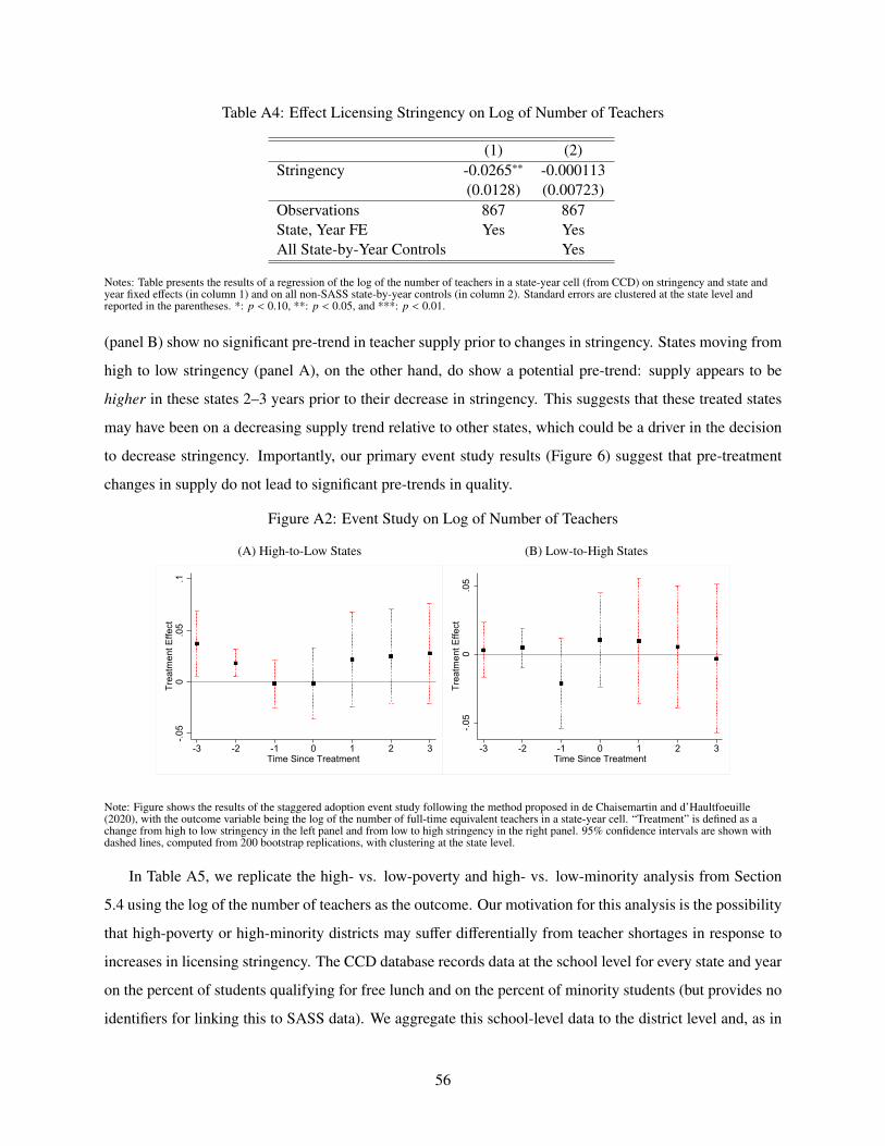
Table A4: Effect Licensing Stringency on Log of Number of Teachers

(1) (2)Stringency -0.0265∗∗ -0.000113

(0.0128) (0.00723)Observations 867 867State, Year FE Yes YesAll State-by-Year Controls Yes

Notes: Table presents the results of a regression of the log of the number of teachers in a state-year cell (from CCD) on stringency and state andyear fixed effects (in column 1) and on all non-SASS state-by-year controls (in column 2). Standard errors are clustered at the state level andreported in the parentheses. *: p < 0.10, **: p < 0.05, and ***: p < 0.01.

(panel B) show no significant pre-trend in teacher supply prior to changes in stringency. States moving from

high to low stringency (panel A), on the other hand, do show a potential pre-trend: supply appears to be

higher in these states 2–3 years prior to their decrease in stringency. This suggests that these treated states

may have been on a decreasing supply trend relative to other states, which could be a driver in the decision

to decrease stringency. Importantly, our primary event study results (Figure 6) suggest that pre-treatment

changes in supply do not lead to significant pre-trends in quality.

Figure A2: Event Study on Log of Number of Teachers

(A) High-to-Low States

-.05

0.0

5.1

Trea

tmen

t Effe

ct


(B) Low-to-High States

-.05

0.0

5Tr

eatm

ent E

ffect


Note: Figure shows the results of the staggered adoption event study following the method proposed in de Chaisemartin and d’Haultfoeuille(2020), with the outcome variable being the log of the number of full-time equivalent teachers in a state-year cell. “Treatment” is defined as achange from high to low stringency in the left panel and from low to high stringency in the right panel. 95% confidence intervals are shown withdashed lines, computed from 200 bootstrap replications, with clustering at the state level.

In Table A5, we replicate the high- vs. low-poverty and high- vs. low-minority analysis from Section

5.4 using the log of the number of teachers as the outcome. Our motivation for this analysis is the possibility

that high-poverty or high-minority districts may suffer differentially from teacher shortages in response to

increases in licensing stringency. The CCD database records data at the school level for every state and year

on the percent of students qualifying for free lunch and on the percent of minority students (but provides no

identifiers for linking this to SASS data). We aggregate this school-level data to the district level and, as in

56

Section 5.4, we construct above-median and below-median indicators for the poverty and minority status of

district observations within a state-year cell. We then aggregate data to the state-by-year-by-poverty-status

level and the state-by-year-by-minority-status level.

Column 1 of Table A5 includes only state and year fixed effects, column 2 includes all non-SASS state-

by-year controls from the preferred specification, and column 3 includes state-by-year fixed effects, which

is feasible because we generally have two observations in a given state-by-year cell in this regression. In

both panels A and B of Table A5, the point estimates for the interaction effects are negative in all specifica-

tions, consistent with the possibility that high-poverty and high-minority school districts experience a larger

decrease in supply than less-vulnerable districts. In column 2, which corresponds most closely to our main

specification in the body of the paper, the 95% confidence interval on the interaction effect for high-poverty

districts rejects decreases of more than 0.2 log points or increases of more than about 0.11. The correspond-

ing confidence interval for the high-minority interaction term is (-0.23,0.15). In all cases, the confidence

intervals on interaction terms also contain zero.

Table A5: Heterogeneous Effects of Licensing Stringency on Log of Number of Teachers

A: Effect for Low- vs. High-Poverty (1) (2) (3)Stringency -0.0307 -0.0153

(0.0484) (0.0509)

High Poverty 0.0160 0.0102 -0.0638(0.0759) (0.0755) (0.112)

Stringency * High Poverty -0.0424 -0.0414 -0.0415(0.0784) (0.0787) (0.120)

Observations 1514 1514 1514

B: Effect for Low- vs. High-Minority (1) (2) (3)Stringency -0.00918 0.0154

(0.0496) (0.0518)

High Minority 0.704∗∗∗ 0.703∗∗∗ 0.694∗∗∗

(0.0912) (0.0918) (0.129)

Stringency * High Minority -0.0403 -0.0411 -0.0434(0.0976) (0.0983) (0.138)

Observations 1608 1608 1608State, Year FE Yes YesAll State-by-Year Controls YesState*Year FE Yes

Notes: Table presents heterogeneous effects of licensing stringency on teacher supply. Each observation is a state-by-year-by-poverty-status cell inpanel A and state-by-year-by-minority-status cell in panel B. The outcome is the log of the number of teachers within the cell. High Poverty andHigh Minority are indicators of whether the cell contains high-poverty districts or high-minority districts within a given state and year. Eachcolumn in each panel corresponds to a separate regression. Controls include state and year fixed effects in column 1, additional non-SASSstate-by-year controls in column 2, and state-by-year fixed effects in column 3. Standard errors are clustered at the state level and reported in theparentheses. *: p < 0.10, **: p < 0.05, and ***: p < 0.01.

57

F Cross-State Mobility

Teachers are required to satisfy the licensing requirements in the state in which they are working, and it is

possible that changes in licensing stringency may affect the state in which teachers choose to work. For

example, college students planning to become teachers may choose a state in which to teach based on the

ease of states’ licensing requirements. This type of cross-state mobility could potentially alter the teacher

quality distribution in a treated state (one that increases stringency) as well as in a control state (one that

leaves stringency unchanged). For example, suppose two states are initially equivalent—in stringency level,

teacher pay, quality distribution, and any other aspect—and suppose one of these states (call it the treated

state) increases its stringency and the other doesn’t, and labor is mobile across states. Some potential

teachers at the upper-tail and lower-tail may be driven out of teaching in the more-stringent state and become

teachers in the less-stringent state, widening the distribution in the less-stringent state, and making the

relative comparison of the distribution of quality between the treated state and untreated state even starker.

This suggests that part of the effects we measure in the body of the paper may be driven by such cross-state

moves.

We can analyze this issue empirically in two ways. First, we can examine whether licensing stringency

affects the fraction of teachers working in a different state than the one in which they attended college. We

can construct this fraction in each state-year cell using the SASS data. We find this fraction to be 23% on

average, suggesting that most teachers teach in the same state in which they attended college. Treating this

23% level as the natural level of in-migration for teachers, we then examine whether this fraction changes

systematically when a state increases its licensing stringency. In panel A of Table A6, we show results from

regressions analogous to those in equation (1) but with this fraction being the dependent variable. We find

no significant effects of stringency on the fraction of teachers teaching in a given state who did not attend

college there, and the confidence intervals are small enough to rule out meaningful effects.

Second, we examine the frequency of the in-migration of teachers into a given state who were previously

teaching in a different state. The SASS data suggests that such moves are very rare to begin with: only 2%

of teachers report having taught in a different state in the previous year. In panel B of Table A6, we use this

fraction as our dependent variable and we use the stringency in the SASS survey year as the right-hand-side

variable of interest.65 We find negative point estimates that are statistically significant, consistent with the

possibility that in-migration is indeed reduced when a state increases licensing restrictions.

In panel C, we examine whether states with higher in-migration rates differ in their teacher quality

65We use the survey-year stringency because a state’s licensing requirements in the survey year are those that a newly arrivingteacher would need to satisfy. Similarly, for any non-SASS controls in this regression (such as controls coming from the CPS), weuse the values corresponding to those in the corresponding SASS survey year.

58

distribution. Here we use regressions similar to those in equation (1) but with the fraction of movers into the

state (from panel B) as the right-hand-side variable of interest rather than stringency. Note that the estimates

in panel C represent the effect of this fraction changing from 0 (no movers) to 1 (100% of teachers being

movers). To interpret these changes in terms of percentage points, the estimates must be divided by 100.

For example, the point estimate on the 10th percentile in column 3 suggests that an increase of 1 percentage

point in the fraction of movers (which corresponds to a 50% increase in the move rate relative to the mean)

is associated with an increase of 0.005 standard deviations in the left tail of quality for secondary school

teachers. This number is small and is also statistically insignificant. We also find no significant relationships

in other specifications in panel C. Thus, while a state’s stringency level does indeed appear to affect the

rate of in-migration of teachers, it does not appear to affect the distribution of quality. Given these results,

and given that the fraction of teachers who cross state borders after they begin teaching is small to begin

with, we do not think cross-state migration in response to stringency changes poses a major problem for the

interpretation of our main results.

Table A6: Effect of Stringency on Teachers Moving States

A. Teach in Diff State than College (1) (2) (3)Stringency -0.00742 -0.0235 0.0184

(0.00778) (0.0165) (0.0156)

B. Teach in Diff State Last Year (1) (2) (3)Stringency -0.00881∗∗∗ -0.00926∗∗ -0.00699∗∗

(0.00275) (0.00379) (0.00315)

C. Quality Regressed on Fraction Movers (1) (2) (3)Average q: Fraction Movers 0.0360 -0.303 0.0690

(0.417) (0.420) (0.411)

10th Percentile q: Fraction Movers 0.493 -0.359 0.545(0.776) (0.672) (0.728)

90th Percentile q: Fraction Movers -0.317 0.231 0.335(0.599) (0.767) (0.566)

Observations 857 696 815Sample All Elem SecAll Controls Yes Yes Yes

Notes: Panels A and B present the results of equation (1) where the left-hand-side variable is the fraction of teachers working in a state differentfrom their undergraduate institution in panel A and the fraction of teachers teaching in a different state than they taught in last year in panel B.Panel B uses stringency in the survey year as the right-hand-side variable of interest. Panel C shows regressions with the same outcomes as inTable 2 but with the right-hand-side variable of interest being the fraction of teachers in a state-year cell who taught in a different state in theprevious year. Each cell in the table corresponds to a different regression. Column 1 shows results for all teachers, column 2 for elementary schoolteachers, and column 3 for secondary school teachers. All regressions include all state-by-year controls, as in the preferred specification (column 7of Table 2). Standard errors are clustered at the state level and reported in the parentheses. *: p < 0.10, **: p < 0.05, and ***: p < 0.01.

This finding is consistent with a number of other papers that have demonstrated that teachers do not

tend to move across state lines. Strauss et al. (2000), studying Pennsylvania teachers, document that 80% of

teachers work within 70 miles of where they attended college, and 40% teach in the precise district where

59

they attended school as a child. Goldhaber et al. (2015), studying teachers in Washington and Oregon,

demonstrate that teachers are very unlikely to travel across states, and they argue that this may be attributable

to pensions structures (i.e., teachers have already invested in a given state’s pension program) or to state

licensing requirements that teachers have already invested in satisfying in their current state (Kim et al. 2017

offer similar findings). This latter argument would suggest that, if anything, stricter licensing requirements

in a given state would be expected to reduce cross-state mobility, consistent with other findings in the

occupational licensing literature more broadly (Johnson and Kleiner 2017). One study (Hirsch 2001) does

document a case of teachers moving across state borders for higher pay (moving from Oklahoma to Texas

in 1999).

G Additional Details on Data Construction

Table A13 lists the sources for each of the 37 teacher licensing requirements for each year. The table

demonstrates that data on some of the 37 certification requirements are missing in some years; additional

requirements beyond the 37 we focus on are also recorded in some manuals but are missing for more years.

For any of the 37 requirements with missing data in 1991 (which only applies to two of the 37 requirements),

we fill in these missing requirements with the next available year. We fill in any other missing requirement-

year cells with the most recent year’s information. Note that when data is available for a given requirement

in a given year, it is always available for all states. Table A13 also displays the mean and standard deviation

of each requirement, computed by taking the mean and standard deviation within each state over time and

then averaging over states.

The Bartik labor demand variable is constructed as follows. For state s and year t, this variable is given

by Bs,d(t) ≡1

100,000∑

k Lskgkd, where Lsk is industry k’s share of employment in state s in 1990 and gkd is the

national wage growth rate of industry k from decade d− 1 to decade d. The notation d(t) denotes the decade

surrounding year t. Therefore, this Bartik measure varies by decade within a given state: for all years from

1991–2000, the Bartik variable is set to the 1991–2000 decade value, and for years from 2001–2008, the

Bartik variable is set to the 2001–2008 decade value. Data for constructing this variable come from the 1990

and 2000 U.S. Census IPUMS data and the 2006–2008 American Community Survey (Flood et al. 2020).

The Klarner (2013a,b) data is coded as follows: for the executive branch, 0 = Republican, 1 = Demo-

cratic, and 0.5 = Independent or other. For the legislative branch, 0 = Republican control of both houses;

0.25 = Republican control of one house, split control of the other; 0.5 = Democratic control of one house,

Republicans control of the other; 0.75 = Democratic control of one house, split control of the other; 1 =

Democratic control of both houses. The Klarner (2013a,b) data, as well as the collective bargaining data,

60

do not contain information on Washington, D.C.; we manually collect these variables for D.C., primarily

from Wikipedia, where we consider the mayor as the executive branch and the Council of the District of

Columbia as the legislative branch.

Appendix References

AACTE (1990, 1991, 1993-1996). Teacher Education Policy in the States: A 50-State Survey of Legislativeand Administrative Actions. American Association of Colleges for Teacher Education, Washington, DC.Six certification manuals.

Athey, S. and Imbens, G. W. (2018). Design-based analysis in difference-in-differences settings with stag-gered adoption. NBER Working Paper 24963.

Borusyak, K. and Jaravel, X. (2017). Revisiting event study designs. Working Paper, available at SSRN2826228.

Boydston, J. E. (1995-2010). Teacher Certification Requirements in All 50 States: How and Where to Geta Teaching Certificate. Teacher Certification Publications, Sebring, FL. Fifteen cerfication manuals from1995 to 1999 and from 2001 to 2010.

Callaway, B. and Sant’Anna, P. H. (2019). Difference-in-differences with multiple time periods. Availableat SSRN 3148250.

de Chaisemartin, C. and D’Haultfœuille, X. (2020a) Difference-in-differences estimators of intertemporaltreatment effects. Working Paper, available at arXiv:2007.04267.

Duncan, A. and Madzelan, D. T. (2009). The secretary’s sixth annual report on teacher quality: A highlyqualified teacher in every classroom. U.S. Department of Education, Office of Postsecondary Education.

Goddard, R. E. (1983-1993). Teacher Certification Requirements in All 50 States: How and Where to Geta Teaching Certificate. Teacher Certification Publications, Grover Hill, OH. Eleven cerfication manualsfrom 1983 to 1993.

Goldhaber, D., Grout, C., Holden, K. L., and Brown, N. (2015). Crossing the border? Exploring the cross-state mobility of the teacher workforce. Educational Researcher, 44(8):421–431.

Goodman-Bacon, A. (2018). Difference-in-differences with variation in treatment timing. NBER WorkingPaper 25018.

Hanushek, E. A., Kain, J. F., and Rivkin, S. G. (2004). Why public schools lose teachers. Journal of HumanResources, 39(2):326–354.

Hirsch, E. (2001). Teacher recruitment: Staffing classrooms with quality teachers. ERIC Paper NumberED453199.

Johnson, J. E. and Kleiner, M. M. (2017). Is occupational licensing a barrier to interstate migration? NBERWorking Paper 24107.

Kim, D., Koedel, C., Ni, S., and Podgursky, M. (2017). Labor market frictions and production efficiency inpublic schools. Economics of Education Review, 60:54–67.

61

Kirby, S. N., Naftel, S., and Berends, M. (1999). Staffing at-risk school districts in texas. problems andprospects. ERIC No. ED436496.

NASDTEC (1991, 1994, 1996, 1998, 2000–2004). National Association of State Directors of Teacher Ed-ucation Certification (NASDTEC) Manual on the Preparation and Certification of Education Personnel.Kendall/Hunt Publishing Company, Dubuque, IA. Seven certification manuals.

NASDTEC Knowledgebase (2003–2010). National Association of State Directors of Teacher EducationCertification (NASDTEC) Manual on the Preparation and Certification of Education Personnel and NAS-DTEC Knowledgebase. Kendall/Hunt Publishing Company, Dubuque, IA. As published on NationalCenter for Education Statistics (NCES) website: http://nces.ed.gov/programs/digest/. Eight tables fromyears 2003-2010.

Northern, A. M., Scull, J., and Zeehandelaar, D. (2012). How strong are US teacher unions? A state-by-statecomparison. Thomas B. Fordham Institute, 18:2018.

Sun, L. and Abraham, S. (2018). Estimating dynamic treatment effects in event studies with heterogeneoustreatment effects. Working paper, arXiv:1804.05785.

62

Figure A3: Additional Event Study Results for Secondary School Teachers

(A) Average Quality, High-to-Low States

-1-.5

0.5

1Tr

eatm

ent E

ffect


(B) 90th Percentile, High-to-Low States

-1-.5

0.5

11.

5Tr

eatm

ent E

ffect


(C) 90th Percentile Low-to-High States

-1.5

-1-.5

0.5

1Tr

eatm

ent E

ffect


Notes: Figure shows the results of the staggered-adoption event study following the method proposed in de Chaisemartin and d’Haultfoeuille(2020), with the outcome variable being the average quality (in panel A) or the 90th percentile (in panels B and C) of teacher quality amongsecondary school teachers within a state-year cell. “Treatment” is defined as a change from high to low stringency in panels A and B, and from lowto high stringency in panel C. 95% confidence intervals are shown with dashed lines, computed from 200 bootstrap replications, with clustering atthe state level.

63

Table A7: Full Coefficient Estimates from Table 2, Col 7, Panel A (All Teachers)

(1) (2) (3)Average q 10th Percentile q 90th Percentile q

Stringency 0.0163 0.141∗∗∗ 0.0413(0.0283) (0.0427) (0.0486)

Fraction Urban Schools 0.390∗∗∗ 0.698∗∗ 0.165(0.109) (0.304) (0.189)

Fraction Suburban Schools 0.271∗∗∗ 0.328 0.352∗

(0.101) (0.245) (0.209)Log Total Enrollment -0.236 -0.189 -0.231

(0.278) (0.661) (0.670)Log State Educ. Expenditure 0.237 0.167 -0.0256

(0.252) (0.531) (0.496)Log No. Charter Schools -0.00650 -0.0150 -0.0243

(0.0110) (0.0302) (0.0204)Average Percent Free Lunch -0.00511∗∗ -0.00426 -0.00226

(0.00196) (0.00419) (0.00310)Average Percent Minority Enrollment -0.000930 -0.00736∗∗ 0.00358

(0.00165) (0.00361) (0.00339)Log Pub. Teacher Earnings (IPUMS) -0.0829 -0.208 -0.0355

(0.100) (0.222) (0.198)Log Pri. Teacher Earnings (IPUMS) -0.0432 0.0330 -0.0932

(0.0309) (0.0552) (0.0726)Frac. Union Member (IPUMS) -0.0824 -0.412 0.854

(0.300) (0.634) (0.526)Log Pri. Teacher Earnings (SASS) -0.000499 -0.00441 0.128

(0.0736) (0.153) (0.148)Pri. Teacher Earnings Exists (SASS) -0.00715 0.0384 -1.318

(0.750) (1.564) (1.494)Log Pub. Teacher Earnings (SASS) 0.358∗ 0.491 -0.0488

(0.200) (0.461) (0.356)Log District BA Salary (SASS) 0.0471 -0.436 -0.151

(0.510) (0.883) (1.020)Log District MA Salary (SASS) -0.308 -0.353 0.451

(0.360) (0.855) (0.839)Fraction Teachers in Union (SASS) -0.233∗ -0.495∗ -0.421

(0.120) (0.289) (0.306)Bartik Shock -0.0646 -0.296 0.661

(0.364) (0.697) (0.776)Log Per-capita Income 0.741 1.820 0.808

(0.570) (1.272) (1.071)Log Average Wage Income -0.149 -0.197 -0.285

(0.194) (0.333) (0.495)Party of Governor 0.0806∗∗∗ 0.0398 0.0585

(0.0190) (0.0466) (0.0521)Party of State Legislature 0.0161 0.153 -0.131

(0.0600) (0.119) (0.0955)Governor is Lame Duck 0.00123 0.113∗ -0.0479

(0.0237) (0.0567) (0.0418)Democrat-Republican Gov. Vote -0.00201∗∗∗ 0.000574 -0.00322∗

(0.000673) (0.00197) (0.00164)Post Financial Adequacy Policy -0.0187 0.0728 0.106

(0.0407) (0.0894) (0.0842)Log No. Desegregation Orders -0.123∗∗∗ -0.110 -0.167∗∗

(0.0408) (0.0714) (0.0646)Collective Bargaining Required -0.282 0.534 -2.145∗∗

(0.500) (1.040) (0.906)Collective Bargaining Allowed -0.356 0.153 -2.138∗∗

(0.499) (1.006) (0.888)Observations 857 857 857

Notes: Table reports most coefficient estimates from column 7 of panel A of Table 2. The full set of unemployment rate controls is omitted to savespace. Each column represents a different regression, where the outcome is a different statistic of the distribution: the mean (column 1), the 10thpercentile (column 2), or the 90th percentile (column 3). Standard errors are clustered at the state level and reported in the parentheses. *:p < 0.10, **: p < 0.05, and ***: p < 0.01.

64

Table A8: Full Coefficient Estimates from Table 2, Col 7, Panel B (Elementary School Teachers)


Stringency -0.000124 0.0433 0.0295(0.0391) (0.0693) (0.0609)

Fraction Urban Schools 0.317∗ 0.467∗∗ 0.426(0.176) (0.219) (0.339)

Fraction Suburban Schools 0.265∗ 0.619∗∗∗ 0.116(0.141) (0.229) (0.265)

Log Total Enrollment 0.379 1.318 1.336∗

(0.464) (0.920) (0.725)Log State Educ. Expenditure -0.0893 -0.287 -0.353

(0.446) (0.753) (0.579)Log No. Charter Schools -0.00548 -0.0125 0.0134

(0.0200) (0.0557) (0.0321)Average Percent Free Lunch -0.00647∗∗ -0.000584 -0.0153∗∗∗

(0.00261) (0.00335) (0.00453)Average Percent Minority Enrollment -0.000841 -0.00719∗∗ 0.00101

(0.00194) (0.00341) (0.00309)Log Pub. Teacher Earnings (IPUMS) -0.00850 -0.432 0.188

(0.157) (0.347) (0.308)Log Pri. Teacher Earnings (IPUMS) -0.0718 -0.0997 -0.187

(0.0598) (0.106) (0.114)Frac. Union Member (IPUMS) -0.664 -1.356 -0.0179

(0.430) (0.845) (0.479)Log Pri. Teacher Earnings (SASS) -0.00645 0.115 -0.0829

(0.0936) (0.178) (0.202)Pri. Teacher Earnings Exists (SASS) 0.0705 -1.238 0.801

(0.955) (1.817) (2.062)Log Pub. Teacher Earnings (SASS) 0.0144 0.468 0.0169

(0.336) (0.317) (0.657)Log District BA Salary (SASS) -0.947 -1.609 -2.479∗

(0.592) (0.988) (1.366)Log District MA Salary (SASS) 0.867 1.459 2.306

(0.823) (1.278) (1.530)Fraction Teachers in Union (SASS) -0.0875 -0.124 -0.231

(0.0861) (0.221) (0.150)Bartik Shock 0.0458 -0.431 0.717

(0.588) (0.839) (1.192)Log Per-capita Income 1.007 3.082∗ 0.940

(0.928) (1.704) (1.651)Log Average Wage Income -0.441∗ -0.834∗ -1.273∗

(0.259) (0.475) (0.650)Party of Governor 0.147∗∗∗ 0.0998 0.204∗∗

(0.0367) (0.0913) (0.0811)Party of State Legislature 0.0292 0.0684 0.147

(0.106) (0.133) (0.170)Governor is Lame Duck -0.00478 -0.00169 -0.0190

(0.0367) (0.0617) (0.0627)Democrat-Republican Gov. Vote -0.00365∗∗∗ -0.00564∗ -0.00683∗∗∗

(0.000971) (0.00286) (0.00173)Post Financial Adequacy Policy -0.0394 -0.119 0.00884

(0.0603) (0.157) (0.0921)Log No. Desegregation Orders -0.120∗∗ -0.232 -0.0864

(0.0580) (0.170) (0.106)Collective Bargaining Required -0.112 -1.810 -1.299

(0.645) (1.683) (1.333)Collective Bargaining Allowed -0.114 -1.962 -1.034

(0.658) (1.633) (1.376)Observations 696 696 696

Notes: Table reports most coefficient estimates from column 7 of panel B of Table 2. The full set of unemployment rate controls is omitted to savespace. Each column represents a different regression, where the outcome is a different statistic of the distribution: the mean (column 1), the 10thpercentile (column 2), or the 90th percentile (column 3). Standard errors are clustered at the state level and reported in the parentheses. *:p < 0.10, **: p < 0.05, and ***: p < 0.01.

65

Table A9: Full Coefficient Estimates from Table 2, Col 7, Panel C (Secondary School Teachers)


Stringency 0.0312 0.140∗∗∗ -0.0328(0.0274) (0.0383) (0.0482)

Fraction Urban Schools 0.267∗ 0.673∗∗∗ -0.282(0.145) (0.240) (0.225)

Fraction Suburban Schools 0.214∗ 0.504∗∗ -0.157(0.121) (0.200) (0.198)

Log Total Enrollment -0.806∗∗∗ -1.194∗∗ -1.232∗∗

(0.282) (0.485) (0.542)Log State Educ. Expenditure 0.407∗∗ 0.609∗ 0.364

(0.189) (0.352) (0.441)Log No. Charter Schools -0.00413 0.00656 -0.00302

(0.0145) (0.0233) (0.0216)Average Percent Free Lunch -0.00118 -0.00294 0.00592

(0.00234) (0.00590) (0.00435)Average Percent Minority Enrollment -0.00365∗∗ -0.0110∗ 0.00359

(0.00150) (0.00654) (0.00296)Log Pub. Teacher Earnings (IPUMS) -0.0349 -0.141 0.210

(0.103) (0.225) (0.221)Log Pri. Teacher Earnings (IPUMS) -0.0344 -0.00766 -0.0328

(0.0326) (0.0658) (0.0682)Frac. Union Member (IPUMS) 0.238 0.228 0.889

(0.323) (0.569) (0.600)Log Pri. Teacher Earnings (SASS) 0.0273 -0.169 0.489∗∗∗

(0.0752) (0.134) (0.127)Pri. Teacher Earnings Exists (SASS) -0.304 1.746 -4.989∗∗∗

(0.776) (1.361) (1.295)Log Pub. Teacher Earnings (SASS) -0.236 -0.102 -0.404

(0.288) (0.551) (0.628)Log District BA Salary (SASS) 0.410 -0.899 1.090

(0.519) (1.377) (0.866)Log District MA Salary (SASS) 0.0877 0.581 -0.529

(0.469) (1.171) (0.930)Fraction Teachers in Union (SASS) -0.156 -0.250∗ -0.386∗

(0.125) (0.143) (0.199)Bartik Shock -0.631 -0.966 -0.945

(0.456) (0.924) (0.767)Log Per-capita Income 0.672 0.882 1.078

(0.533) (1.112) (1.059)Log Average Wage Income 0.196 0.731∗ -0.103

(0.237) (0.409) (0.387)Party of Governor 0.0629∗∗ 0.0755∗ 0.0217

(0.0264) (0.0441) (0.0664)Party of State Legislature -0.0135 0.134 -0.0856

(0.0462) (0.0917) (0.0906)Governor is Lame Duck 0.00844 0.137∗ -0.00669

(0.0277) (0.0794) (0.0476)Democrat-Republican Gov. Vote -0.00117∗ 0.000287 -0.00156

(0.000637) (0.00170) (0.00167)Post Financial Adequacy Policy -0.0207 0.102 -0.0264

(0.0365) (0.0741) (0.0886)Log No. Desegregation Orders -0.168∗∗∗ -0.0693 -0.172∗

(0.0413) (0.0939) (0.0862)Collective Bargaining Required -0.877 -1.318 -1.090

(0.632) (1.532) (1.283)Collective Bargaining Allowed -0.864 -1.603 -0.967

(0.647) (1.568) (1.288)Observations 815 815 815

Notes: Table reports most coefficient estimates from column 7 of panel C of Table 2. The full set of unemployment rate controls is omitted to savespace. Each column represents a different regression, where the outcome is a different statistic of the distribution: the mean (column 1), the 10thpercentile (column 2), or the 90th percentile (column 3). Standard errors are clustered at the state level and reported in the parentheses. *:p < 0.10, **: p < 0.05, and ***: p < 0.01.

66

Table A10: Heterogeneous Effects of Stringency on Quality Distribution, State-by-Year Fixed Effects

Average Quality 10th Percentile 90th PercentileA: High Poverty (1) (2) (3) (4) (5) (6) (7) (8) (9)High Poverty -0.176∗∗∗ -0.187∗∗∗ -0.177∗∗∗ -0.284∗∗ -0.298∗∗ -0.240∗∗∗ -0.113 -0.138∗∗ -0.0903

(0.0564) (0.0655) (0.0622) (0.106) (0.125) (0.0842) (0.0798) (0.0544) (0.128)

Str.*High Poverty -0.00409 0.0160 -0.0185 -0.0899 -0.0530 -0.0640 -0.0586 0.0157 -0.0174(0.0393) (0.0582) (0.0472) (0.0680) (0.0801) (0.0818) (0.0535) (0.0631) (0.0847)

Observations 1572 1268 1500 1572 1268 1500 1572 1268 1500

B: High Minority (1) (2) (3) (4) (5) (6) (7) (8) (9)High Minority -0.0947∗ -0.0905 -0.0764 -0.349∗∗∗ -0.328∗∗ -0.322∗∗∗ 0.0671 0.0778 0.179∗∗

(0.0515) (0.0766) (0.0616) (0.111) (0.139) (0.116) (0.0516) (0.0827) (0.0867)

Str.*High Minority -0.0299 -0.0372 -0.0240 -0.0549 -0.0945 -0.00303 0.0191 -0.0325 0.00417(0.0339) (0.0490) (0.0531) (0.0717) (0.0852) (0.0891) (0.0365) (0.0658) (0.0527)

Observations 1704 1373 1620 1704 1373 1620 1704 1373 1620

Sample All Elem Sec All Elem Sec All Elem SecState*Year FE Yes Yes Yes Yes Yes Yes Yes Yes Yes

Notes: Table presents heterogeneous effects of licensing stringency on the teacher quality, estimated from equation (2) but with state-by-year fixedeffects included. Each observation in the underlying regressions is a state-by-year-by-poverty-status cell (for panel A) or astate-by-year-by-minority-status cell (for panel B). The outcome is the mean (in columns 1–3), 10th percentile (in columns 4–6), or 90th percentile(in columns 7–9) of teacher quality within the cell. High Poverty and High Minority are indicators of whether the cell contains high-povertydistricts or high-minority districts within a given state and year. “Str.” stands for stringency. Each column in each panel corresponds to a separateregression. Columns 1, 4, and 7 show results for all teachers; columns 2, 5, and 8 restrict to elementary school teachers; and columns 3, 6, and 9restrict to secondary school teachers. Standard errors are clustered at the state level and reported in the parentheses. *: p < 0.10, **: p < 0.05, and***: p < 0.01.

Table A11: Effects of Second and Third Factors on Quality Distribution, State & Year Fixed Effects Only

(1) (2) (3) (4) (5) (6)Average q: Stringency 0.0190 -0.0102 0.0552 0.0142 0.0211 0.00901

(0.0336) (0.0544) (0.0350) (0.0236) (0.0282) (0.0324)

10th Percentile q: Stringency 0.0512 -0.114 0.120∗ 0.0797 0.0207 0.105(0.0586) (0.102) (0.0637) (0.0484) (0.0516) (0.0766)

90th Percentile q: Stringency 0.0786 -0.0129 0.117 -0.000670 -0.0170 0.0341(0.0602) (0.0897) (0.0730) (0.0423) (0.0573) (0.0456)

Observations 857 696 815 857 696 815Principal Factor Factor 2 Factor 2 Factor 2 Factor 3 Factor 3 Factor 3Sample All Elem Sec All Elem SecState, Year FE Yes Yes Yes Yes Yes Yes

Notes: Table presents the baseline specification (corresponding to column 1 from Table 2, where only state and year fixed effects are included) butwith the main stringency metric replaced with the second factor (in columns 1–3) or third factor (in columns 4–6) from the principal factoranalysis. Each cell in the table corresponds to a different regression and the reported coefficient is the effect of licensing stringency. Columns 1 and4 use the all-teachers sample, columns 2 and 5 use elementary school teachers, and columns 3 and 6 use secondary school teachers. Standarderrors are clustered at the state level and reported in the parentheses. *: p < 0.10, **: p < 0.05, and ***: p < 0.01.

67

Figure A4: Loadings of Certification Requirements on Second Factor

●●

●●

●●

●●●●●●●●●●●●●

●●●●●

●●●

●●●

●●●

●●●●

−0.39

−0.34

−0.31

−0.22

−0.09

−0.08

−0.05

−0.01

−0.01

0

0.01

0.01

0.02

0.02

0.04

0.04

0.05

0.07

0.07

0.12

0.12

0.14

0.15

0.15

0.18

0.19

0.2

0.23

0.24

0.25

0.33

0.36

0.37

0.45

0.45

0.47

0.47

BA From Accredited InstitutionMust Be Professional Educ Major

General Education CourseworkBA From State−Approved Institution

Fee RequirementU.S. Citizenship

Oath of AllegianceEnglish Coursework

Humanities CourseworkMath Coursework

Natural Science CourseworkSocial Science Coursework

General Health CertificateGeneral Knowledge ExamStudies of Subject Matter

Knowledge of US and/or State ConstitutionStudent Teaching Hour Requirement

TB Test or Chest X−RayOther G.E. Coursework Requirement

Knowledge of Teaching ExamRecommendation (College / Employer)

Minimum Age RequirementBA From Regionally Accredited Institution

FingerprintingField Experience Before Student Teaching

Must Not Be Professional Educ MajorEvidence of Employment

Screening for Moral CharacterHealth Drug Alcohol Training

Basic Skill ExamComputer Education Training

Special Education TrainingState Student Teacher EvaluationState Subject Matter Requirement

Nutrition TrainingSubject Matter Exam

Assessment of Teaching Performance

−0.25 0.00 0.25 0.50

Loadings

Notes: Figure displays the factor loading of each of the 37 licensing requirements used in the Principal Factor Analysis (PFA) on the secondcomponent.

68

Figure A5: Loadings of Certification Requirements on Third Factor

●●

●●

●●●●

●●●●●●●●●

●●●●●●

●●●●●

●●

●●●

●●

●●

−0.46

−0.4

−0.36

−0.28

−0.24

−0.22

−0.2

−0.19

−0.09

−0.04

−0.04

−0.04

−0.03

−0.01

−0.01

0.01

0.02

0.05

0.06

0.06

0.07

0.08

0.09

0.15

0.15

0.15

0.17

0.17

0.22

0.24

0.28

0.29

0.31

0.36

0.39

0.43

0.45

Special Education TrainingHealth Drug Alcohol TrainingComputer Education Training

Field Experience Before Student TeachingFee Requirement

Recommendation (College / Employer)BA From State−Approved Institution

Screening for Moral CharacterNutrition Training

Must Not Be Professional Educ MajorEvidence of EmploymentStudies of Subject Matter

Humanities CourseworkState Subject Matter Requirement

Math CourseworkOther G.E. Coursework Requirement

BA From Accredited InstitutionFingerprinting

Natural Science CourseworkEnglish Coursework

General Education CourseworkBA From Regionally Accredited Institution

Social Science CourseworkStudent Teaching Hour Requirement

TB Test or Chest X−RayMust Be Professional Educ Major

Knowledge of US and/or State ConstitutionBasic Skill Exam

Minimum Age RequirementState Student Teacher Evaluation

General Health CertificateOath of Allegiance

Assessment of Teaching PerformanceU.S. Citizenship

General Knowledge ExamSubject Matter Exam

Knowledge of Teaching Exam

−0.50 −0.25 0.00 0.25

Loadings

Notes: Figure display the factor loading of each of the 37 licensing requirements used in the Principal Factor Analysis (PFA) on the thirdcomponent.

69

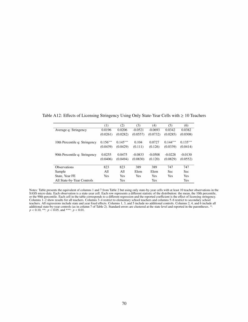
Table A12: Effects of Licensing Stringency Using Only State-Year Cells with ≥ 10 Teachers

(1) (2) (3) (4) (5) (6)Average q: Stringency 0.0196 0.0206 -0.0521 -0.0693 0.0342 0.0382

(0.0261) (0.0282) (0.0557) (0.0732) (0.0285) (0.0308)

10th Percentile q: Stringency 0.156∗∗∗ 0.145∗∗∗ 0.104 0.0727 0.144∗∗∗ 0.135∗∗∗

(0.0439) (0.0429) (0.111) (0.126) (0.0339) (0.0414)

90th Percentile q: Stringency 0.0255 0.0475 -0.0833 -0.0508 -0.0228 -0.0130(0.0406) (0.0494) (0.0830) (0.120) (0.0829) (0.0552)

Observations 823 823 389 389 747 747Sample All All Elem Elem Sec SecState, Year FE Yes Yes Yes Yes Yes YesAll State-by-Year Controls Yes Yes Yes

Notes: Table presents the equivalent of columns 1 and 7 from Table 2 but using only state-by-year cells with at least 10 teacher observations in theSASS micro data. Each observation is a state-year cell. Each row represents a different statistic of the distribution: the mean, the 10th percentile,or the 90th percentile. Each cell in the table corresponds to a different regression and the reported coefficient is the effect of licensing stringency.Columns 1–2 show results for all teachers. Columns 3–4 restrict to elementary school teachers and columns 5–6 restrict to secondary schoolteachers. All regressions include state and year fixed effects. Columns 1, 3, and 5 include no additional controls. Columns 2, 4, and 6 include alladditional state-by-year controls (as in column 7 of Table 2). Standard errors are clustered at the state level and reported in the parentheses. *:p < 0.10, **: p < 0.05, and ***: p < 0.01.

70

Figure A6: Additional Figures

(A) Avg SAT Score vs Earnings by Undergrad. Institution

2000

040

000

6000

080

000

Avg.

Ear

ning

s 6

Year

s Af

ter E

nter

ing

Col

lege

800 1000 1200 1400 1600Average SAT Score of Admitted Students

(B) Scree Plot of Eigenvalues

02

46

Eige

nval

ues

0 10 20 30 40Number of Factors

(C) Leave-One-Out, State & Year FE

050

100

150

200

250

Den

sity

.13 .14 .15 .16 .17Effect of Stringency on 0.1 Quantile with 1 State Removed

(D) Leave-One-Out, All Controls

050

100

150

Den

sity

.1 .12 .14 .16 .18Effect of Stringency on 0.1 Quantile with 1 State Removed

Notes: Panel A displays a local quadratic regression fit between average earnings (in 2007 dollars) six years after entering college (vertical axis)and average SAT score of admitted students (horizontal axis). An observation is an undergraduate institution observed in collegescorecard.ed.govdata. Panel B, referred to as a scree plot, shows the eigenvalues of each factor from the principal factor analysis of the teacher licensingrequirements. Panels C and D show histograms of the effect of licensing stringency on the 10th percentile of teacher quality for secondary schoolteachers, estimated from equation (1), leaving out one state at a time. Panel C regressions use only state and year fixed effects and panel Dregressions include all controls from the preferred specification.

71

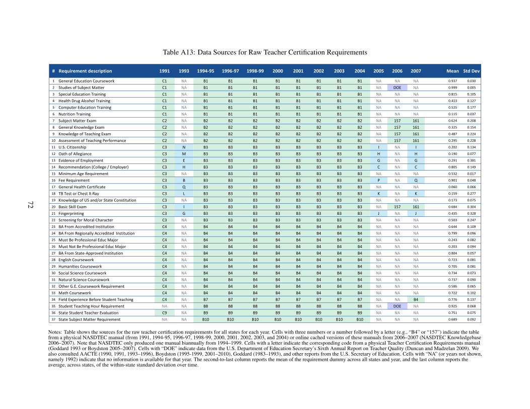
Table A13: Data Sources for Raw Teacher Certification Requirements

# Requirement description 1991 1993 1994-95 1996-97 1998-99 2000 2001 2002 2003 2004 2005 2006 2007 Mean Std Dev

1 General Education Coursework C1 NA B1 B1 B1 B1 B1 B1 B1 B1 NA NA NA 0.937 0.030

2 Studies of Subject Matter C1 NA B1 B1 B1 B1 B1 B1 B1 B1 NA DOE NA 0.999 0.005

3 Special Education Training C1 NA B1 B1 B1 B1 B1 B1 B1 B1 NA NA NA 0.815 0.105

4 Health Drug Alcohol Training C1 NA B1 B1 B1 B1 B1 B1 B1 B1 NA NA NA 0.413 0.127

5 Computer Education Training C1 NA B1 B1 B1 B1 B1 B1 B1 B1 NA NA NA 0.525 0.177

6 Nutrition Training C1 NA B1 B1 B1 B1 B1 B1 B1 B1 NA NA NA 0.115 0.037

7 Subject Matter Exam C2 NA B2 B2 B2 B2 B2 B2 B2 B2 NA 157 161 0.624 0.208

8 General Knowledge Exam C2 NA B2 B2 B2 B2 B2 B2 B2 B2 NA 157 161 0.325 0.154

9 Knowledge of Teaching Exam C2 NA B2 B2 B2 B2 B2 B2 B2 B2 NA 157 161 0.487 0.224

10 Assessment of Teaching Performance C2 NA B2 B2 B2 B2 B2 B2 B2 B2 NA 157 161 0.295 0.228

11 U.S. Citizenship C3 N B3 B3 B3 B3 B3 B3 B3 B3 I NA I 0.202 0.134

12 Oath of Allegiance C3 M B3 B3 B3 B3 B3 B3 B3 B3 H NA H 0.190 0.077

13 Evidence of Employment C3 E B3 B3 B3 B3 B3 B3 B3 B3 G NA G 0.291 0.381

14 Recommendation (College / Employer) C3 H B3 B3 B3 B3 B3 B3 B3 B3 C NA C 0.805 0.149

15 Minimum Age Requirement C3 NA B3 B3 B3 B3 B3 B3 B3 B3 NA NA NA 0.532 0.017

16 Fee Requirement C3 B B3 B3 B3 B3 B3 B3 B3 B3 P NA Q 0.901 0.048

17 General Health Certificate C3 Q B3 B3 B3 B3 B3 B3 B3 B3 NA NA NA 0.060 0.066

18 TB Test or Chest X-Ray C3 L B3 B3 B3 B3 B3 B3 B3 B3 K NA K 0.159 0.277

19 Knowledge of US and/or State Constitution C3 NA B3 B3 B3 B3 B3 B3 B3 B3 NA NA NA 0.173 0.075

20 Basic Skill Exam C3 I B3 B3 B3 B3 B3 B3 B3 B3 NA 157 161 0.684 0.304

21 Fingerprinting C3 G B3 B3 B3 B3 B3 B3 B3 B3 J NA J 0.435 0.328

22 Screening for Moral Character C3 NA B3 B3 B3 B3 B3 B3 B3 B3 NA NA NA 0.503 0.247

23 BA From Accredited Institution C4 NA B4 B4 B4 B4 B4 B4 B4 B4 NA NA NA 0.644 0.109

24 BA From Regionally Accredited Institution C4 NA B4 B4 B4 B4 B4 B4 B4 B4 NA NA NA 0.799 0.096

25 Must Be Professional Educ Major C4 NA B4 B4 B4 B4 B4 B4 B4 B4 NA NA NA 0.243 0.082

26 Must Not Be Professional Educ Major C4 NA B4 B4 B4 B4 B4 B4 B4 B4 NA NA NA 0.203 0.094

27 BA From State-Approved Institution C4 NA B4 B4 B4 B4 B4 B4 B4 B4 NA NA NA 0.804 0.057

28 English Coursework C4 NA B4 B4 B4 B4 B4 B4 B4 B4 NA NA NA 0.723 0.081

29 Humanities Coursework C4 NA B4 B4 B4 B4 B4 B4 B4 B4 NA NA NA 0.705 0.081

30 Social Science Coursework C4 NA B4 B4 B4 B4 B4 B4 B4 B4 NA NA NA 0.734 0.073

31 Natural Science Coursework C4 NA B4 B4 B4 B4 B4 B4 B4 B4 NA NA NA 0.737 0.090

32 Other G.E. Coursework Requirement C4 NA B4 B4 B4 B4 B4 B4 B4 B4 NA NA NA 0.586 0.065

33 Math Coursework C4 NA B4 B4 B4 B4 B4 B4 B4 B4 NA NA NA 0.722 0.102

34 Field Experience Before Student Teaching C4 NA B7 B7 B7 B7 B7 B7 B7 B7 NA NA B4 0.776 0.137

35 Student Teaching Hour Requirement NA NA B8 B8 B8 B8 B8 B8 B8 B8 NA DOE NA 0.925 0.068

36 State Student Teacher Evaluation C9 NA B9 B9 B9 B9 B9 B9 B9 B9 NA NA NA 0.751 0.075

37 State Subject Matter Requirement NA NA B10 B10 B10 B10 B10 B10 B10 B10 NA NA NA 0.689 0.092

Notes: Table shows the sources for the raw teacher certification requirements for all states for each year. Cells with three numbers or a number followed by a letter (e.g., “B4” or “157”) indicate the tablefrom a physical NASDTEC manual (from 1991, 1994-95, 1996-97, 1998-99, 2000, 2001, 2002, 2003, and 2004) or online cached versions of these manuals from 2006–2007 (NASDTEC Knowledgebase2006–2007). Note that NASDTEC only produced one manual biannually from 1994–1999. Cells with a letter indicate the corresponding code from a physical Teacher Certification Requirements manual(Goddard 1993 or Boydston 2005–2007). Cells with “DOE” indicate data from the U.S. Department of Education Secretary’s Sixth Annual Report on Teacher Quality (Duncan and Madzelan 2009). Wealso consulted AACTE (1990, 1991, 1993–1996), Boydston (1995-1999, 2001–2010), Goddard (1983–1993), and other reports from the U.S. Secretary of Education. Cells with “NA” (or years not shown,namely 1992) indicate that no information is available for that year. The second-to-last column reports the mean of the requirement dummy across all states and year, and the last column reports theaverage, across states, of the within-state standard deviation over time.

72

The E ect of Occupational Licensing Stringency on the ...

Documents

Transcript of The E ect of Occupational Licensing Stringency on the ...