The Dynamics of Cognition:

An ACT-R Model of Cognitive Arithmetic

Christian LebiereNovember 23, 1998CMU-CS-98-186

School of Computer ScienceComputer Science DepartmentCarnegie Mellon University

Pittsburgh, PA

Submitted in partial fulfillment of the requirementsfor the degree of Doctor of Philosophy

Thesis Committee:

John R. Anderson, ChairBonnie JohnTom Mitchell

Robert Siegler, Psychology Department, Carnegie Mellon University

1998 Christian Lebiere

This research was sponsored by the Office of Naval Research under contract numberN00014-95-10223 to John Anderson at Carnegie Mellon University. The views andconclusions contained in this document are those of the author and should not beinterpreted as representing the official policies, either expressed or implied, of the ONRor the U.S. government.

Keywords: ACT-R, cognitive arithmetic, Bayesian learning, activation spreading,

dynamical systems, parameter analysis, power law, machine learning, hybrid systems.

iii

Abstract

Cognitive arithmetic, the study of the mental representation of numbers and

arithmetic facts and the processes that create, access and manipulate them, offers a

unique window into human cognition. Unlike traditional Artificial Intelligence (AI)

tasks, cognitive arithmetic is trivial for computers but requires years of formal training

for humans to master. Understanding the basic assumptions of the human cognitive

system which make such a simple and well-understood task so challenging might in turn

help us understand how humans perform other, more complex tasks and engineer systems

to emulate them. The wealth of psychological data on every aspect of human

performance of arithmetic makes precise computational modeling of the detailed error

and latency patterns of cognitive arithmetic the best way to achieve that goal.

While specialized models have been quite successful at accounting for many

aspects of cognitive arithmetic, this thesis aims to provide an integrated model of the

field using a general-purpose cognitive modeling architecture (ACT-R). This model

makes minimal assumptions but instead relies on the architecture’s Bayesian learning

mechanisms to derive the desired results from the statistical structure of the task. The

behavior of this model is analyzed using several approaches: separate simulations of each

main result, a single simulation of a lifetime of arithmetic learning, a formal analysis of

the model’s dynamics and an empirical variation of the simulation’s parameters.

This thesis provides a unifying account of the main results of cognitive arithmetic.

Through its parameter analysis, it suggests some practical lessons for the teaching of

arithmetic. The constraints of a lifetime simulation of arithmetic learning also expose the

underlying assumptions of ACT-R’s associative learning mechanism. While a

simplifying assumption commonly used in machine learning is shown in this case to be

inadequate, a more powerful algorithm closely replicates human behavior. The formal

and empirical analyses of the model parameters establish that despite its less-than-perfect

performance, human cognition is surprisingly optimal. Finally, the behavior of the

simulation through a lifetime of arithmetic learning can best be described as a dynamical

system affected not only by its external environment but also by its internal dynamics.

iv

v

Dedicated to the memory of my father,

and the promise of my son.

vi

vii

Table of Contents

CHAPTER 1: INTRODUCTION 1

CHAPTER 2: MODEL AND DATA 6

2.1 ACT-R 6

2.2 Model 102.2.1 Basic Representation and Productions 102.2.2 Sub-symbolic Processes 15

2.3 Data 182.3.1 Problem Size Effect 182.3.2 Errors in Addition Retrieval 222.3.3 Errors in Multiplication Computation 26

CHAPTER 3: LEARNING OVER TIME 29

3.1 Problem Size Effect over Time 29

3.2 Learning the Correct Answer 323.2.1 Overview 323.2.2 Basic Dynamics of Error Odds 363.2.3 Context and Complexity 383.2.4 Matching Penalty 403.2.5 Multiple Alternatives 403.2.6 External Feedback Sources 413.2.7 Comparison 42

CHAPTER 4: THE LIFETIME SIMULATION 44

4.1 Model 45

4.2 Results 50

4.3 Associative Strengths and Interference 564.3.1 General Introduction 564.3.2 Tie Problems 594.3.3 Near-tie Problems 634.4.4 Corner Problems 644.3.5 Cross-type Interference 664.3.6 A More General Solution 67

4.4 Retrieval as Subgoaling 71

viii

CHAPTER 5: PARAMETER SENSITIVITY 74

5.1 Introduction 74

5.2 Activation Noise 76

5.3 Retrieval Threshold 79

5.4 Mismatch Penalty 82

5.5 Presentation Schedule 85

5.6 Steepness of Frequency Distribution 88

5.7 Feedback Probability 93

5.8 Discussion 97

CHAPTER 6: DISCUSSION 101

6.1 Feeling of Knowing 101

6.2 Strategy Choice 103

6.3 Multiplication Errors 107

CHAPTER 7: CONCLUSION 113

7.1 Difficulties 113

7.2 Contributions 114

TABLES 117

Table 1: Equations 117

Table 2: Symbols 118

Table 3: Parameters 120

APPENDIX 121

REFERENCES 123

ix

Acknowledgments

This thesis started with the support of my family, and their repeated encouragement that

this was something worth doing. My wife Theresa provided her love and her relentless

determination in getting things done. I will be forever thankful to her for putting up with

me. My father-in-law ceaselessly sang the virtues of education. My son Mathieu was the

source of endless distractions, and so many reminders that there are more important

things too. I want to thank them all for their love and support.

The ACT-R group at Carnegie Mellon and beyond provided much of the intellectual

background to this work. The discussions in the hallway, at the weekly Friday research

meeting, and at the yearly ACT-R workshop were the testing-bench on which these ideas

were refined. I want to thank in particular Dieter Wallach for those extraordinarily

stimulating few months we spent as officemates. Science is indeed a cooperative

endeavor.

I would like to thank my committee for guiding me and asking all the right questions.

Tom Mitchell lent a benevolent but always insightful ear. Bob Siegler provided

encyclopedic knowledge of the field. Ever since the first ACT-R summer school, Bonnie

John has always asked the tough architectural questions, and never taken no for an

answer.

Most importantly, I want to thank my advisor, John Anderson, for giving me this

opportunity. He showed me how research is done and allowed me to be productive.

Without him this thesis would never have seen the light of day.

x

1

Chapter 1: Introduction

Cognitive arithmetic studies the mental representation of numbers and arithmetic facts

(counting, addition, subtraction, multiplication, division) and the processes that create,

access and manipulate them. Arithmetic is one of the fundamental cognitive tasks (one

of the three basic “R”s) which humans have to master. Children go through years of

formal schooling to learn, first the numbers, then the facts and skills needed to

manipulate them. Many adults have not and will never completely master the domain.

And yet it is a task that is trivial to perform correctly for computer architectures.

Some tasks, such as natural language processing or chess, are hard for both humans and

machines to perform and require years of learning or engineering. Other tasks, such as

vision, which seem to come naturally to humans, require much programming for

computers to perform even poorly. One can attribute that to humans possessing a

complex vision system which resulted from millions of years of evolution but will require

painstaking work to reverse-engineer and replicate in computers. But a task such as

arithmetic seems so straightforward and easy to accomplish that it is surprising that it

takes years of learning for humans to master. This suggests that human cognition at the

most basic level embodies some assumptions about its environment that are at odds with

the structure of arithmetic as it is taught. Arithmetic, being a formal mathematical

theory, assumes a set of precise and immutable objects (the numbers), facts, and

procedures. Human cognition, on the other hand, has evolved to deal with approximate

concepts, changing facts, and adaptive procedures. Studying how such a system deals

with a formal task such as arithmetic provides an excellent window to its assumptions

and mechanisms.

ACT-R is a hybrid production-system theory of human cognition (Anderson, 1993;

Anderson & Lebiere, 1998). At the symbolic level, ACT-R is a fairly standard goal-

directed production system, with a declarative memory of long-term facts, known as

2

chunks, and a procedural memory holding general production rules. At that level,

cognitive arithmetic is a trivial task for ACT-R. All one needs to do is give ACT-R the

correct chunks representing arithmetic facts and productions encoding procedures to

manipulate them and perfect performance will result. This, however, ignores the impact

of ACT-R’s sub-symbolic level and would not be a very satisfactory model of human,

especially children's, performance. ACT-R is also an activation-based system in which

the performance at the symbolic level is controlled by associated real-valued quantities.

Those quantities are learned according to Bayesian principles to reflect the architecture’s

environment. Retrieval and matching of memory chunks by production rules is a noisy,

approximate process driven by activation rather than the exact matching of conditions.

Thus the behavior of the system becomes adaptive, stochastic and error-prone, matching

human behavior better but making cognitive arithmetic a more challenging, but also more

interesting task.

Cognitive arithmetic is a task that is both well suited and challenging to ACT-R for a

number of reasons. Unlike tasks artificially designed for the purpose of isolating a

particular cognitive mechanism, the learning and performance of arithmetic involves

almost every mechanism of the architecture. It is therefore an excellent test of whether

these parts can perform together as well as separately. Unlike laboratory tasks, large

amounts of data are available for every cross-section of the population and every aspect

of the task, making it easier to establish the trends being analyzed.

While numbers can be seen as having a concrete interpretation (e.g. children learn the

concept "three" by being shown three rabbits), the rest of arithmetic has essentially an

abstract structure. It is much less likely that people have brain structures optimized to

perform arithmetic than for example vision or language, and suggests a complete reliance

on general-purpose learning mechanisms. Since each skill builds on the previous ones,

e.g. counting can be used to perform addition, which in turn can be used to perform

multiplication, learning can thus be a mostly self-contained process, rather than entirely

dependent upon external factors such as teaching. Arithmetic also has an inherently

clear, simple and regular structure, with a systematic organization of knowledge into

3

tables of immutable facts. This strong regularity, unlike for example the many

exceptions of tasks such as natural language processing, also helps in reducing degrees of

freedom in modeling the task and provides a good test of ACT-R's statistical learning.

These factors lead to a simpler, more regular model that is more predictive than one with

many unanalyzed degrees of freedom.

There are two classes of empirical phenomena in the domain of arithmetic that any model

needs to account for. One concerns the fact that children, and to a certain degree adults,

approach answering arithmetic problems with two basic strategies. One strategy is to

simply retrieve the answer. The second strategy, referred to hereafter as the backup

strategy or backup computation, is to compute the answer. Thus, given a problem such as

3 + 4 = ? children may choose to count (perhaps 4, 5, 6, 7) to provide the answer and

given 3 * 4 = ? they may choose to add to get the answer (perhaps 4 + 4 + 4). One class

of empirical phenomena involves how people choose between the computation strategy

and the retrieval strategy.

The second class of empirical phenomena involves the problem-size effect. Children and

adults take longer to answer problems involving larger numbers and they also make more

errors on these problems. In the case of backup computation the reason for this is fairly

obvious -- one has to count more to add large numbers and one has to add more things

when multiplying by a larger number. However, while much reduced, the problem-size

effect occurs for adults. It has been suggested that this is due to residual use of the

backup strategy (LeFevre, et. al., 1996a), although recent research put those results in

doubt (Kirk & Ashcraft, 1997). However, it has been argued that smaller problems also

occur more often, offering greater practice. This is true in studies of textbooks (Ashcraft,

1987; Ashcraft & Christy, 1995; Hamman & Ashcraft, 1986; Siegler, 1988) but it is also

true in the world at large. As many (Benford, 1938; Newcomb, 1888; Raimi, 1976) have

noted, small numbers occur more often in the world generally. As just one interesting

token of the ubiquity of small numbers, consider the addition problems created by adding

the two rows in multiplication problems involving two-digit numbers. An example is

given below:

4

46x 83 138368 .3818

The problem creates a 3+8 addition problem and a 1+ 6 addition problem. If one looks at

all such multiplication problems with multiplicands from 10 to 99, one finds that addition

problems involving smaller addends occur more frequently. Figure 1.1 plots, as a

function of the size of the addend, the frequency of all additions problems created by

adding the tens digit from the top row (i.e. 138) with the ones digit from the bottom row

(i.e. 368) or the hundreds digit from the top row with the tens digit from the bottom row.

There is a clear drop off with size of the addend.1

1 0864201000

2000

3000

4000

5000

6000

7000

1-Digit Addition from 2-digit Multiplication

Addend

Fre

quen

cy

Figure 1.1: Frequency of 1-digit Addition ProblemsCreated by 2-digit Multiplication Problems.

1 The drop-off with size of addend on Figure 1.1 happens because the hundreds digit inthese addition problems tends to be small and the saw-tooth pattern is produced becausethe ones digit is more often even.

5

These effects of problem size and strategy are ubiquitous throughout the literature on

cognitive arithmetic (for reviews of the field, see e.g. Ashcraft, 1992, 1995; Campbell,

1995; Geary, 1996). While these effects are not by far the only ones to account for, they

constitute a good basis for a comprehensive model of cognitive arithmetic. In a model of

Zbrodoff's alphabet arithmetic experiment (Anderson & Lebiere, 1998), it was shown that

ACT-R had the ability to account for these effects in the miniature. However, it is

another question whether, when ACT-R's learning mechanisms are turned on and given a

lifetime of experience, the resulting behavior will look at all like human behavior. This is

the challenge that this thesis is trying to address.

Chapter 2 describes the basic model and its ability to account for basic results in the field

of cognitive arithmetic. These demonstrations will be typical “mini-models” which

assume a certain distribution of knowledge strength at a particular point in time. Chapter

3 analyzes how to go beyond those limited models in creating a model that gradually

improves its performance with practice. Chapter 4 presents such a model, called the

lifetime simulation, which like human students goes through the equivalent of years of

training while replicating the results that were previously modeled separately. From the

difficult constraints imposed by the lifetime simulation will be derived a number of

lessons for the use and evolution of the architecture. Chapter 5 analyzes the sensitivity of

the lifetime simulation to its parameters and draw conclusions regarding the nature of

human cognition and the teaching of arithmetic. Chapter 6 discusses some issues

concerning cognitive arithmetic, including the feeling of knowing, the question of

strategy selection and the nature of human guessing. Chapter 7 summarizes the

difficulties encountered in this endeavor and the contributions made by this thesis.

6

Chapter 2: Model and Data

2.1 ACT-R

ACT-R is an activation-based goal-directed production system theory (Anderson, 1993;

Anderson & Lebiere, 1998). Knowledge in ACT-R is divided into declarative knowledge

stored in chunks (e.g. arithmetic facts) and procedural knowledge stored in productions

(e.g. how to retrieve a fact given a problem). Sub-symbolic activation processes control

which productions are used and how they apply to chunks. The parameters of these

numerical processes reflect the past statistics of use of the knowledge structures to which

they are attached. They are learned by Bayesian learning mechanisms derived from the

rational analysis of cognition (Anderson, 1990). The equations governing this sub-

symbolic level will be described below and are summarized in Table 1 and 2.

In ACT-R, the activation of a declarative memory element, or chunk, can be interpreted

as reflecting the log posterior odds that the chunk is relevant in the current context. The

activation of a chunk is the sum of the base-level activation of that chunk plus the sum

for all context elements of their attentional weights (a.k.a. activation source level) times

the strength of association between the context element and the chunk. In Bayesian

terms, the base-level activation represents the log prior odds of the chunk being relevant

and the strength of association represents the log likelihood ratio that the chunk is

relevant given the context element.

Formally, the activation Ai of chunk i is defined as:

A B W Si i jj

ji= + ∑ Activation Equation

where Bi is the base level activation of i, Wj is the attentional weight given the focus

7

element j, and Sji is the strength of association (a.k.a. Interactive Association or IA

values) from element j to chunk i. An element j is in the focus, or in context, if it is a part

of the current goal, and the total amount of attention is divided evenly among goal

elements.

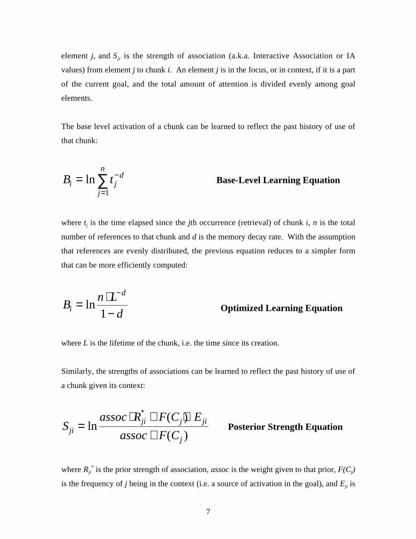
The base level activation of a chunk can be learned to reflect the past history of use of

that chunk:

B ti jd

j

n

= −

=∑ln

1

Base-Level Learning Equation

where tj is the time elapsed since the jth occurrence (retrieval) of chunk i, n is the total

number of references to that chunk and d is the memory decay rate. With the assumption

that references are evenly distributed, the previous equation reduces to a simpler form

that can be more efficiently computed:

Bn L

di

d

= ⋅−

−ln

1 Optimized Learning Equation

where L is the lifetime of the chunk, i.e. the time since its creation.

Similarly, the strengths of associations can be learned to reflect the past history of use of

a chunk given its context:

Sassoc R F C E

assoc F Cjiji j ji

j

=⋅ + ⋅

+

∗

ln( )

( ) Posterior Strength Equation

where Rji* is the prior strength of association, assoc is the weight given to that prior, F(Cj)

is the frequency of j being in the context (i.e. a source of activation in the goal), and Eji is

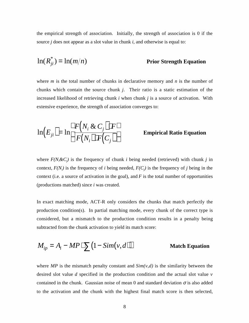
8

the empirical strength of association. Initially, the strength of association is 0 if the

source j does not appear as a slot value in chunk i, and otherwise is equal to:

ln( ) ln( )*R m nji = Prior Strength Equation

where m is the total number of chunks in declarative memory and n is the number of

chunks which contain the source chunk j. Their ratio is a static estimation of the

increased likelihood of retrieving chunk i when chunk j is a source of activation. With

extensive experience, the strength of association converges to:

ln ln&

EF N C F

F N F Cjii j

i j( ) =

( ) ⋅

( ) ⋅ ( )

Empirical Ratio Equation

where F(Ni&Cj) is the frequency of chunk i being needed (retrieved) with chunk j in

context, F(Ni) is the frequency of i being needed, F(Cj) is the frequency of j being in the

context (i.e. a source of activation in the goal), and F is the total number of opportunities

(productions matched) since i was created.

In exact matching mode, ACT-R only considers the chunks that match perfectly the

production condition(s). In partial matching mode, every chunk of the correct type is

considered, but a mismatch to the production condition results in a penalty being

subtracted from the chunk activation to yield its match score:

M A MP Sim v dip i= − ⋅ − ( )( )∑ 1 , Match Equation

where MP is the mismatch penalty constant and Sim(v,d) is the similarity between the

desired slot value d specified in the production condition and the actual slot value v

contained in the chunk. Gaussian noise of mean 0 and standard deviation σ is also added

to the activation and the chunk with the highest final match score is then selected,

9

assuming that it reaches the retrieval threshold τ. If one approximates the Gaussian noise

with a sigmoid distribution, the probability P of chunk i being retrieved by production p

is:

Pe

Mips

=+ −

−1

1τ Retrieval Probability Equation

where s=√3σ/π.. If no chunk reaches the retrieval threshold, then a retrieval failure

occurs and the next production is selected. If more than one chunk is competing for

retrieval, the probability P(i) of chunk i being the one that is retrieved follows the

Boltzmann equation, i.e.:

P ie

e

Mt

Mt

j

ip

jp( ) =

∑ Chunk Choice Equation

where t=√2s. The latency Timeip to retrieve (match) a chunk i with production p is an

exponentially decreasing function of the sum of the chunk’s match score and the

production strength Sp (which, like a chunk’s base level, is a reflection of the frequency

of use of the production):

Time Feipf M Sip p= − +( )

Retrieval Time Equation

where F is a time scaling constant and f an activation scaling constant usually left to its

default value of 1 (i.e. ignored). The productions that can apply to the current focus of

attention are matched in sequence by decreasing value of expected gain E:

10

E PG C= − Expected Gain Equation

where G is the value of the current goal, P is its ultimate probability of success given this

production firing and C is the cost of execution of this and following productions until

completion of the goal. Gaussian noise is added to the expected gain value, and thus

production selection will also be stochastic and follow the Boltzmann distribution. The

probability and cost parameters can also be learned according to the record of success and

failure of each production. The reader should consult Anderson & Lebiere (1998) for

additional details of the ACT-R theory. More information about ACT-R, including the

models that are presented in this thesis, is available on the ACT-R web site at

http://act.psy.cmu.edu.

2.2 Model

This section will set forth the basic model of cognitive arithmetic. There is nothing

particularly novel in the types of chunks and productions that were chosen. They reflect

a common approach in the ACT-R community and are already used to model many

phenomena.

2.2.1 Basic Representation and Productions

Arithmetic problems are represented as chunks with four slots: one for the operator, one

for each operand and one for the result. For example, the chunk representing the fact that

2+3=5 would be:

Fact-2+3=5isa arithmeticfirst 2operator +second 3result 5

11

where 2, +, 3 and 5 are other chunks representing the numbers and operator.2 The most

basic action that one can perform on knowledge chunks is to retrieve them. This is

accomplished by the Retrieval production, which solves an arithmetic problem by simply

retrieving the answer to the problem stored in long-term memory:

Retrieval=goal>

isa arithmeticfirst =firstoperator =operatorsecond =secondresult nil

=fact>isa arithmeticfirst =firstoperator =operatorsecond =secondresult =answer

==>=goal>

result =answer

This production simply retrieves a chunk (fact) matching the goal (problem), then copies

the answer back to the goal. One can notice that the chunk retrieved from memory is of

the same type as the goal representing the problem, and wonder how the fact was initially

created. In ACT-R 4.0, there are only two possibilities. The first is that it results from

the encoding of an environmental stimulus. In this case, this would correspond to an

external source of arithmetic knowledge such as a teacher, a table from a book, or a

calculator. The second possibility is the long-term encoding of a past goal. If one cannot

retrieve a fact one can (re)generate the arithmetic knowledge by the use of backup

computation strategies. An example of such a strategy, which is to perform an addition

by repeatedly counting up from one argument a number of times equal to the second

argument, can be implemented by the production Iteration :

2 Although addition and multiplication are commutative operations, this is not reflected inthe declarative representation of facts, i.e. 2+3=5 and 3+2=5 are represented as separatechunks. Of course, this does not prevent explicit procedures to exploit the inherentcommutativity, e.g. solve the problem 2+3=? by retrieving the fact 3+2=5.

12

Iteration=goal>

isa arithmeticfirst =firstoperator +second =secondresult nil

==>=subgoal>

isa iterateresult =firstcounter 0limit =secondincrement 1result =answer

!push! =subgoal=goal>

result =answer

This production solves an addition problem by setting a subgoal to iteratively add the

second argument to the first by increments of 1, using the basic counting skills. Table 2.1

shows the two production rules that were used to accomplish this iterative counting

procedure. This counting subgoal is pushed on the stack, and its result will be returned to

the current goal as the answer to the problem using the subgoal value return mechanism.

When an answer to the problem has been found using either retrieval or one of the

backup strategies, the answer is output and the goal is popped by the Answer production:

Answer=goal>

isa arithmeticfirst =firstoperator =operatorsecond =secondresult =answer

==>!output! =answer!pop!

When the goal is popped, it becomes a fact in long-term memory. If this fact did not

already exist, then the solving of this problem (presumably using the backup strategies)

has added a new arithmetic fact to the knowledge base. If an identical fact already

13

existed (modulo the chunk name3), then the new chunk is merged with the existing one,

reinforcing it, and the duplicate copy is removed from declarative memory. If the

problem could not be solved by retrieval, this reinforcement from the merging with the

new problem will raise the activation of the fact until ultimately the problem can be

solved by retrieval. If the problem was already solved by retrieving the fact, then it will

receive two learning reinforcements: first, from its use in the retrieval production and,

second, from being merged with the problem goal.

Iterate-count =goal> isa iterate counter =counter - limit =counter result =result increment 1 =fact1> isa count number =counter next =next-counter =fact2> isa count number =result next =next-result==> =goal> counter =next-counter result =next-result

Done =goal> isa iterate counter =counter limit =counter==> !pop!

Table 2.1: Productions for Addition by Iterative Counting.

3 This, together with the rather dubious meaning of whichever name happens to beassociated with such facts, suggests that chunk names are superfluous and that chunkscould be best understood as the content of their slots rather than referred to by name.

14

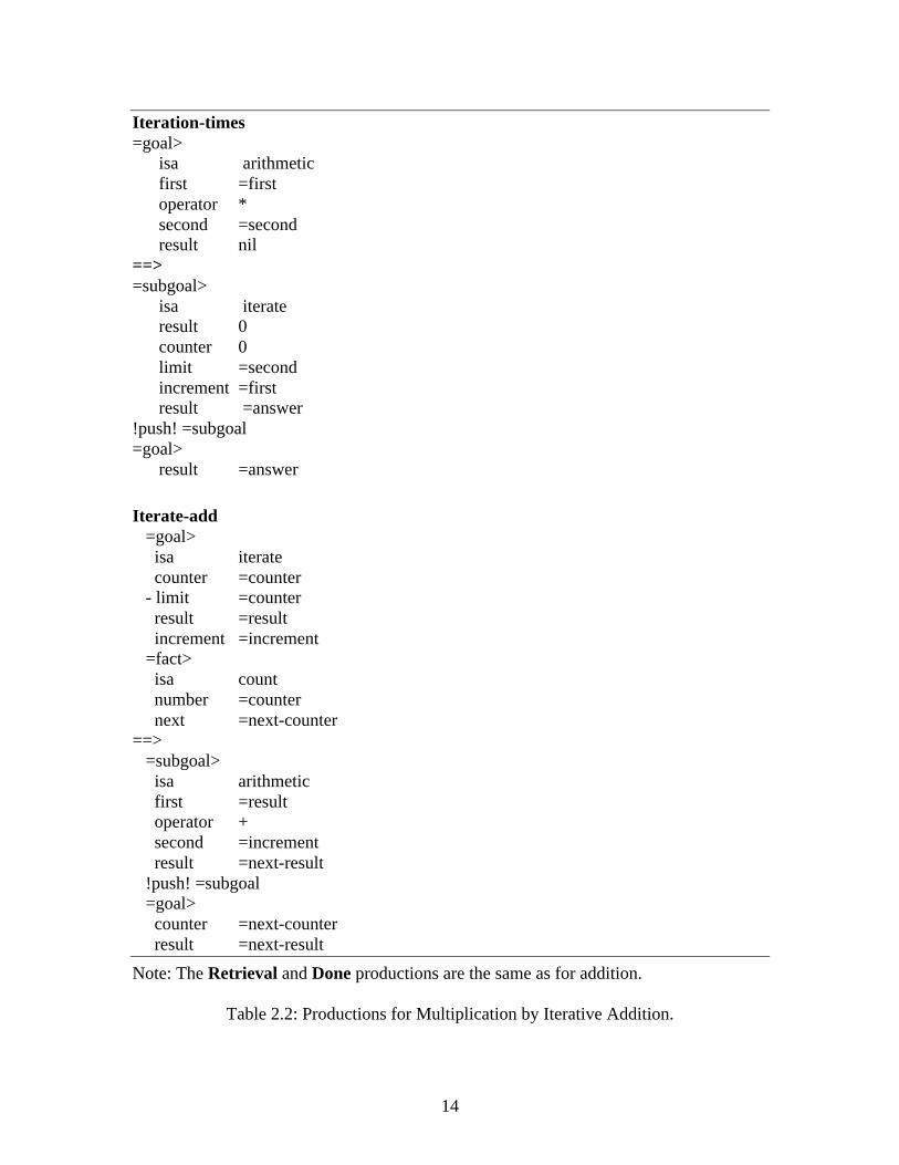
Iteration-times=goal>

isa arithmeticfirst =firstoperator *second =secondresult nil

==>=subgoal>

isa iterateresult 0counter 0limit =secondincrement =firstresult =answer

!push! =subgoal=goal>

result =answer

Iterate-add =goal> isa iterate counter =counter - limit =counter result =result increment =increment =fact> isa count number =counter next =next-counter==> =subgoal> isa arithmetic first =result operator + second =increment result =next-result !push! =subgoal =goal> counter =next-counter result =next-result

Note: The Retrieval and Done productions are the same as for addition.

Table 2.2: Productions for Multiplication by Iterative Addition.

15

Since past goals are the only source of chunks (other than for environmental encoding),

this technique of solving a problem by pushing a goal which can be solved either by

directly retrieving the answer from the corresponding fact or by using a number of

backup strategies is a general ACT-R technique to model problem-solving. By gradually

raising the activation of the necessary facts with practice, it provides a general account of

the transition from general problem-solving strategies toward more efficient ones. As

noted in (Anderson & Lebiere, 1998), ACT-R implements Logan’s (1988) proposal for

transition from algorithmic solutions to direct retrieval.

The discussion has focused on addition but a parallel model for multiplication has been

developed. The iterative addition procedure, corresponding to the counting procedure, is

given in Table 2.2. The productions there try to retrieve the multiplication answers and if

they fail call on a backup strategy of repeated addition.

2.2.2 Sub-symbolic Processes

Since the retrieval and iteration productions (and possibly other backup strategies) share

the same goal condition, conflict resolution is needed to determine which productions are

fired in which order. Typically (and this may not be true for, say, small children), the

retrieval production provides a high probability of producing a correct answer at low cost,

and thus will have the highest evaluation and will be attempted first. If no arithmetic fact

for that problem is above threshold, the retrieval production will time out and the next

production in the conflict resolution order, e.g. iteration, will be allowed to fire.

A general observation is that children will choose to retrieve more often for smaller

problems and choose to compute more often for larger problems (Siegler, 1988). The

simplest explanation for this in ACT-R is that subjects cannot retrieve the answer in the

case of large problems and fall back on computation. This would occur more often for

larger problems because they have less practice (e.g., Figure 1.1). Of course, for people

with a poor knowledge of the facts and a fairly reliable backup strategy, the expected gain

of the retrieval production might well be lower than the expected gain for the backup

16

production(s). In general, people may evolve complex sets of strategies for making the

decision between retrieve and compute. However, let us ignore these complications and

simply assume that the two strategies are retrieve and compute. Moreover, to the extent

that retrieve is preferred in conflict resolution, subjects will only choose to compute after

they have failed to retrieve the answer. This preference for retrieval as the first way of

solving the goal can be seen as an instance of the Obligatory Retrieval Assumption of

Logan (1988), i.e. people cannot help but try to retrieve the answer to an arithmetic

problem and only resort to explicit computation when that fails. Those issues will be

examined in detail in Chapter 6.

Clearly, the activation of chunks storing arithmetic facts is going to be very critical to

ACT-R's performance in cognitive arithmetic. The activation of a chunk is given as a

sum of a base-level activation and associative activation according to the Activation

Equation. The base-level activation will change with experience according to the Base-

Level Learning Equation in such a way that it grows approximately as a log function of

amount of practice. The strengths of association will change with experience according

to the Posterior Learning Equation such that it will come to vary approximately as a log

function of the odds of a chunk being retrieved when another is in the context.

These activation quantities are converted into match scores that reflect the effects of

partial matching (Match Equation). In the case of a perfect match, the match score is just

the activation but in the case of a mismatch a penalty will be subtracted from the match

score. There is noise in these match scores because of activation noise. If the match

score is above a threshold the chunk will be retrievable and the probability of it being

retrieved (rather than some other chunk) is described by the Retrieval Probability

Equation. If there are multiple possible chunks that might match the one chosen is the

one with the highest match score and the probability of any one being chosen is described

by the Chunk Choice Equation. Finally, match scores determine latency through the

Retrieval Time Equation.

Errors can be committed whether the subject is computing or retrieving. Let us consider

17

the example of the problem 2+3=?. Because of ACT-R’s partial matching process it is

possible for ACT-R to retrieve an arithmetic chunk (e.g. 2+4=6) other than the correct

one. Recall that chunks are retrieved on the basis of their match scores that are calculated

as their activation levels minus mismatch scores. It is possible that even after the

mismatch score is subtracted off, the wrong chunk will have the highest match score and

be retrieved instead and its answer stored in the current goal. In this model, the mismatch

penalty between numbers increases linearly as a function of the difference between the

two numbers. Thus, the mismatch penalty between numbers i and j is D*|i-j| where D is

a scale factor to be estimated. The mismatch measure essentially encodes the

representational similarity between numbers.4 This assumption about the representation

of numbers has also been adopted in a number of other models of numerical memory

(Anderson, Spoher & Bennett, 1992; Campbell, 1995; McCloskey & Lindemann, 1992).

Errors can also occur using the backup procedure when the iteration subgoal returns an

erroneous answer because of a misretrieval, a procedural error or any other reason. The

erroneous answer will also be stored in the goal. In both cases of retrieval and

computation errors, not only will the answer to this particular problem be wrong, but the

goal holding the incorrect answer is popped and becomes an erroneous long-term fact

(here, 2+3=6).5 This fact can then be retrieved as the answer to future problems and

perpetuate the error. This otherwise correct retrieval of an erroneous fact becomes

another source of error. This competition between memories for both correct and

erroneous answers is quite similar to Siegler’s treatment (e.g. Siegler, 1988). It might

seem possible that ACT-R could reach an unfortunate state where it has so practiced the

wrong facts that it comes to believe them. Indeed this can occur and the next chapter

describes what must be true for ACT-R to avoid getting absorbed into such error states.

4 Past models have been relatively insensitive to the exact form of the mismatch measure,but Whalen (1996) argues that the internal representation of numerical magnitude is notuniform and influences performance of numerical tasks. The lifetime simulation usessuch a measure where similarities are proportional to the ratio between numbers insteadof their difference.5 This assumes that error correction, provided by another procedure, a teacher or a

18

2.3 Data

This section will examine how this ACT-R model can account for a wide range of effects

in cognitive arithmetic, including the problem-size effect and the patterns of errors in

retrieval and computation of addition and multiplication problems. Even though these

effects typically have multiple, complex sources, simplifying assumptions were made for

the sake of analysis. The lifetime simulation will eliminate the simplifying assumptions

and account for these effects in a more complex manner. The basic import of the results

presented here is that even a fairly simple approach can successfully account for those

effects. The methodology will be as follows: given a data set describing the performance

of human subjects at a particular point in life (e.g. 4-year-olds, 4th graders, adults) on a

particular task (e.g. addition retrieval, multiplication computation) for a particular

measure (e.g. latency, error percentage), assumptions will be made about the distribution

of knowledge at that point in time (e.g. amount of practice) and about the value of the

simulation parameters, and the relevant part of the model (e.g. if the task is retrieval, then

the computation productions will not be used) will be run to provide the model’s

predictions. Again, the lifetime simulation will model all those data sets in a single

simulation with the same set of parameters and assumptions. The parameters used in

those simulations are summarized in Table 3.

2.3.1 Problem Size Effect

The most basic and robust effect in cognitive arithmetic is that larger problems are

harder. This holds for measures of retrieval time and error rates, for the four basic

operations, for production and verification tasks, and for the entire age span from

children to adults and elderly (e.g. Ashcraft, 1992). Ashcraft (1987) reports the change in

response time for addition problems in adults. Figure 2.1 illustrates the relationship

between the sum of the digits and retrieval time. While most problems exhibit an

increase in response time roughly corresponding to the square of the sum of their

operands, the slope for problems involving a zero operand (squares in the graph) is

calculator, does not take effect before the goal is popped and becomes a long-term fact.

19

approximately flat, and the increase in response time for tie problems (those having

identical operands - triangles in the graph) is much smaller than for non-zero, non-tie

problems (circles in the graph). The effect therefore reflects a more complex measure of

problem difficulty than simply problem size.

2 01 000.6

0.8

1.0

1.2

1.4

1.6

1.8

Tie(Data)Zero(Data)

Other(Data)Tie (Model)Zero (Model)

Other (Model)

Problem Size Effect

Sum

RT

(se

c)

Figure 2.1: Problem Size Effect for Addition for Adults: The data are the open points andthe predictions of ACT-R are the closed points connected by lines.

The flat response time for problems involving zero is usually assumed to be the result of

a special-purpose rule for those problems (“0+x=x=x+0 for all x”). This will be modeled

by the use of the special Zero production. Two main explanations have emerged to

account for the rest of the data. Groen and Parkman (1972) initially argued that the

problem size effect resulted from the use of backup strategies such as iterative counting.

Larger problems involve more counting and therefore higher latencies and more errors.

If the first number is always added to the second (or vice versa), then the latency will

increase linearly with the sum of the numbers. A better fitting model, called the min

model, assumes instead that the smaller number is always added to the larger one, thereby

minimizing the number of increments necessary. While this model certainly explains

20

part of the problem size effect for children and other poorly trained subjects, it has

difficulties in fully accounting for the effect in well-trained adults as well as the better

performance on tie problems.

The other category of models relies on the difference of presentation frequency between

problems. As was noted earlier, smaller problems occur more frequently than larger

ones. Smaller problems are therefore easier because they are presented and practiced

more often. Ashcraft (1987) presents the frequency of presentation of addition facts by

operand in grades K to 3 and Siegler (1988) presents the frequency of multiplication

problems in second- and third-grade workbooks. In each case the frequency decreases

roughly linearly with operand size, except for very small operands which are special

cases. It is generally assumed that the distribution in schoolbooks approximately reflects

the real-life problem distribution. This frequency information was used in an ACT-R

simulation whose results are illustrated as lines in Figure 2.1. The ratio of frequencies of

the smallest (0+0) to the largest (9+9) was set at 4-to-1 and intermediate problems had a

frequency that varied linearly with each operand. Thus, if 0+0 occurred four times, 0+9

and 9+0 would occur twice, and 9+9 would occur once.6 This distribution approximates

closely the occurrence frequency in textbooks as described by Hamman and Ashcraft

(1986). This simulation assumes that five hundred thousand problems were presented

according to these frequencies at an average of a hundred problems a day. The

underlying equation determining latency, based on the Retrieval Time Equation, is:

Time I Fe A= + −

where I is an intercept reflecting encoding/answering times, F is the latency factor from

the Retrieval Time Equation, and A is the activation of the chunk encoding the addition

fact. The activation was determined by the half-million trials of experience in ACT-R.

In the model I was estimated at 0.4 second and F was left at the default value of 1.0. An

additional latency of 0.5 second was also estimated for the Zero production. As can be

6 The relative frequency of a problem involving digits i and j was (2 - i/9) (2 - j/9).

21

seen in Figure 2.1 the model does a pretty good job of capturing the effects in the data.

The basic increase in latency with problem size comes from ACT-R's base-level learning.

It follows from the simplified form of the Base-Level Learning and Retrieval Time

Equations that retrieval time is a power function of frequency, and since frequency

decreases roughly linearly with problem size, then the response time for arithmetic

retrieval grows as a power function of problem size.

The retrieval time for the zero operand problems is constant at 0.9 second while it

increases slowly for tie problems to about 1.15 second for the largest problem. Tie

problems generate additional spreading activation in ACT-R because one of the

arguments appears twice in the context. This can be explained by looking at the addition

facts 3+3 and 3+4, and comparing the Sji values learned according to the Posterior

Strength Equation from the number 3 to a tie arithmetic fact (3+3=6) and a non-tie

arithmetic fact (e.g. 3+4=7). In this case j is the number 3 and i is the fact. Assuming for

simplicity that the two facts (3 + 3 = 6 and 3 + 4 = 7) are equally frequently needed, then

all the components of the equation for the two facts are equal except for F(Ni&Cj), which

is double for the tie fact because 3 is twice in the goal context for each retrieval, resulting

in Sji values larger by ln(2) for tie facts. This additional activation spread to tie facts will

in turn result in a decrease of their retrieval latency. Thus, the advantage of tie problems

is a parameter-free prediction of ACT-R’s mechanisms for associative learning.7

This simple model largely relies on differential presentation frequencies to produce the

problem size effect. As will be seen later, differential frequencies of rehearsal (small

problems are retrieved and thus reinforced before larger ones) and backup strategies

(recomputing larger facts is more error-prone than smaller ones) also contribute to the

problem size effect. Finally, even for adults part of the effect may result from the

residual use of non-retrieval procedures (LeFevre et al, 1996a, but see Kirk & Ashcraft,

7It is also possible that subjects encode tie problems using a special representation toreflect their unusual character (data supporting this conclusion is presented by (Eliaser,Siegler, Campbell, & Lemaire, 1997)), which would affect the activation calculus as wellas matching procedures. Finally, tie problems are often assumed to appear morefrequently than indicated by their size alone, although that is not used in the simulation.

22

1997). As mentioned previously, the lifetime simulation will take all these factors into

account and determine their relative importance.

2.3.2 Errors in Addition Retrieval

Table 2.3 presents the pattern of retrieval errors of addition facts by 4-year-olds found by

Siegler and Shrager (1984). The subjects were presented with addition problems ranging

from 1+1 to 5+5 and were asked to just state what they thought the answer was, without

resorting to any overt strategy such as putting up fingers or counting. The main effect,

similar to the problem size effect, is an increase in errors for larger facts. The facts

showing a comparatively low percentage of errors are those involving the operand 1, tie

problems, and problems where the first operand is larger than the second one. Erroneous

answers also tend to be smaller than the correct answer.

0 1 2 3 4 5 6 7 8 9 10 11 other1+1 0 5 86 0 2 0 2 0 0 0 0 2 41+2 0 0 9 70 2 0 4 0 0 7 2 2 51+3 0 2 0 11 71 5 2 2 0 0 0 0 71+4 0 0 0 0 11 61 9 7 0 0 0 2 111+5 0 0 0 0 13 16 50 11 0 2 2 0 52+1 0 7 5 79 5 0 0 0 0 0 0 0 42+2 2 0 4 5 80 4 0 5 0 0 0 0 02+3 0 0 4 7 38 34 9 2 2 2 0 0 42+4 0 2 0 7 2 43 29 7 7 0 0 0 42+5 0 2 0 5 2 16 43 13 0 0 2 0 183+1 0 2 0 9 79 4 0 4 0 0 0 0 43+2 0 0 9 11 11 55 7 0 0 0 0 0 73+3 4 0 0 5 21 9 48 0 2 2 2 0 73+4 0 0 0 5 11 23 14 29 2 0 0 0 163+5 0 0 0 7 0 13 23 14 18 0 5 0 204+1 0 0 4 2 9 68 2 2 7 0 0 0 74+2 0 0 7 9 0 20 36 13 7 0 2 0 74+3 0 0 0 5 18 9 9 38 9 0 2 0 114+4 4 0 0 2 2 29 7 7 34 0 4 0 134+5 0 0 0 0 4 9 16 9 11 18 11 4 205+1 0 0 4 0 4 7 71 4 4 0 4 0 45+2 0 0 5 20 2 18 27 25 2 0 2 0 05+3 0 0 2 11 9 18 5 16 23 0 5 0 115+4 0 0 0 0 11 21 16 5 11 16 4 0 165+5 4 0 0 0 0 7 25 11 2 4 34 4 11

Table 2.3: Retrieval Frequencies for 5x5 Addition Retrieval in 4-year-olds.

Since according to instructions the children were asked not to use any procedure other

23

than retrieval, the computation productions in the model were disabled. Although

guessing and other such procedures could be considered, the basic mechanism for

producing an arithmetic error in ACT-R is the mistaken retrieval of another partially

matching fact (see Match Equation). According to the Chunk Choice Equation, the

probability of such commission errors is proportional to the scaled activation of the

intruding facts relative to the correct fact. Since activation is related to frequency, the

frequency difference between problems8 is therefore critical to explaining the patterns of

errors. The other factor is that partial matching penalties will be smaller among similar

addition facts.

In the case of the retrieval of addition facts, small sums (especially those involving 1,

which can be reduced to the well-practiced skill of counting) are practiced at a higher

frequency and are therefore more likely to intrude upon another problem, leading to an

error for that problem, than to be intruded upon. This higher activation for smaller facts

also explains why the errors for larger facts tend to be biased toward numbers smaller

than the correct answer. Tie problems receive an additional amount of activation, as

described in the previous section, and are therefore more likely to be retrieved correctly.

Finally, let us assume a small probability that, given a problem where the first operand is

smaller than the second one (e.g. 2+4), students reverse the order of arguments to

simplify counting (the min strategy) and therefore also rehearse the reverse answer

(4+2=6), giving it an advantage. The results are shown in Table 2.4. The model

generates answer probabilities that are very close to the data.

This model assumes a thousand problem presentations (an average of 40 for each of the

25 problems in Table 9.3) with a distribution frequency ratio (between smallest and

largest problems) of 6.259, an activation noise s parameter of 0.15, a scaling mismatch

penalty factor of .15 per digit difference10 and a retrieval threshold11 τ of -2.25. The

8Again, this difference can arise from presentation, rehearsal, and computation processes.9 A ratio of 6.25 rather than 4 as in the previous simulation was used to reflect theassumption that young children have a steeper distribution of frequencies than do adults.10This corresponds to the default value of 1.5 for ACT-R's mismatch penalty scalingparameter.

24

strategy of swapping arguments to make sure that the first is larger than the second (and

therefore the extra rehearsals to facts of that type) is modeled by an additional probability

of presentation of those problems that has also been estimated at 6%.

0 1 2 3 4 5 6 7 8 9 10 11 other1+1 0 0 97 2 0 0 0 0 0 0 0 0 01+2 0 0 30 62 7 0 0 0 0 0 0 0 01+3 0 0 28 9 60 2 1 0 0 0 0 0 01+4 0 0 25 9 6 57 1 0 0 0 0 0 11+5 0 0 24 8 6 4 55 1 0 0 0 0 32+1 0 0 20 75 5 0 0 0 0 0 0 0 02+2 0 0 0 16 83 1 0 0 0 0 0 0 02+3 0 0 1 24 38 33 3 0 0 0 0 0 12+4 0 0 1 25 29 15 27 1 0 0 0 0 32+5 0 0 1 26 30 5 13 18 0 0 0 0 73+1 0 0 15 10 73 2 0 0 0 0 0 0 03+2 0 0 1 17 35 44 3 0 0 0 0 0 13+3 0 0 0 0 21 9 70 1 0 0 0 0 03+4 0 0 0 3 24 20 21 26 1 0 0 0 53+5 0 0 1 3 26 11 27 4 14 0 0 0 144+1 0 0 14 9 7 69 1 0 0 0 0 0 14+2 0 0 1 18 21 22 37 1 0 0 0 0 24+3 0 0 1 2 19 22 18 34 1 0 0 0 44+4 0 0 0 0 0 31 11 8 47 0 0 0 14+5 0 0 1 2 3 21 16 7 8 14 0 0 285+1 0 0 14 9 7 5 63 1 0 0 0 0 25+2 0 0 1 19 22 6 19 27 1 0 0 0 55+3 0 0 1 2 20 9 27 6 24 0 0 0 115+4 0 0 1 2 2 18 18 8 8 20 0 0 245+5 0 0 0 0 0 0 47 13 9 6 18 0 7

Table 2.4: Retrieval Frequencies for 5x5 Addition in Model.

Another way to examine this data is to plot the probability of correct retrieval for each

argument as is done in Figure 2.2. Both plots show a fairly close match, with the jump in

percentage correct for problems involving 1, and the greater slope of the addend curve

resulting from the probability of swapping arguments to further favor smaller addends.

11Answers in the “other” category are assumed to be retrieval failures resulting inguessing outside the 0-to-10 range.

25

654321020

30

40

50

60

70

80

DataModel

Addition Retrieval (Augend)

Augend

Per

cent

age

Cor

rect

654321020

30

40

50

60

70

80

DataModel

Addition Retrieval (Addend)

Addend

Per

cent

age

Cor

rect

Figure 2.2: Percentage of Correct Retrievals in Addition: (a) Augend; (b) Addend.

26

As was mentioned in the overview, this is a somewhat simplified model in that it assumes

that only correct facts can be retrieved, albeit sometimes incorrectly. Of course, 4-year-

olds may also hold some incorrect addition facts (at least weakly encoded), which if

correctly retrieved will lead to error (or conversely if incorrectly retrieved could

potentially yield a correct answer). In fact, the incorrect answers generated by the

model's answer to this experiment would lead to just such incorrect facts. Another source

of such errors could be results from past attempts at trying to reconstruct unavailable

addition facts through counting (on their fingers or mentally) or other strategies. It is

however not necessary to specify such past history since the basic assumptions of partial

matching and a difference in rehearsal frequency can lead to a satisfactory model.

2.3.3 Errors in Multiplication Computation

Figure 2.3 from Siegler (1988) presents the percentage of errors in multiplication by

repeated addition, a standard backup computation, for fourth-graders. Subjects were

given single-digit multiplication problems in the form of a column of numbers in which

the multiplicand was repeated the number of times specified by the multiplier, e.g. 8x6

was presented as a column in which 8 was written 6 times. Subjects were asked to add

the columns of numbers and write down the answer. Analogous to the addition problems,

the probability of error increases with the size of both the multiplicand and the multiplier.

Particularly remarkable is the very low percentage of errors for repeated addition of 5.

Since multiplication by repeated addition essentially involves the same retrieval of

arithmetic facts (counting and addition), the same mechanism can also explain that

pattern of errors. Error percentage increases with the size of the multiplier because of the

increase in the opportunities for retrieval error, and with the size of the multiplicand

because of the increased probability of error in the retrieval of larger facts. The

particularly low percentage of errors for repeated addition by 5 is obtained since only two

facts are needed (0+5=5 and 5+5=10) and repeatedly reinforced, unlike other repeated

additions where 5 or all 10 of the facts on that row of the addition table are needed.

27

1 086420

10

20

30

40

50

DataModel

Multiplication Computation (Multiplicand)

Multiplicand

Err

or

Per

cent

age

1 086420

10

20

30

40

50

Data

Model

Multiplication Computation (Multiplier)

Mul t ip l ie r

Err

or

Per

cent

age

Figure 2.3: Percentage of Errors in Multiplication by Repeated Addition.(a) Multiplicand; (b) Multiplier.

28

Figure 2.3 compares the predictions of the model with the data. Since the subjects were

fourth-graders, this model assumes about four years of presentation of addition facts at a

rate of a hundred a day, for a total of about one hundred and fifty thousand. The

frequency ratio of this distribution is 4. In addition, it is assumed that subjects have

previously solved a certain number of multiplication problems by repeated addition. The

distribution of multiplication problems is the one reported by Siegler for second- and

third-grade textbooks. About a thousand multiplication problems are used resulting in

five thousand additional addition rehearsals. The activation noise parameter s is 0.12 and

the same standard mismatch penalty factor of 0.15 per digit as used in the addition

retrieval model. The plot by multiplicand shows a general increase in error percentage

with the size of the argument, resulting from the decrease in rehearsal frequency for

larger problems, and very few errors for addition by 5, resulting from the limited set of

facts needed (and, incidentally, the fact that they both contain the number 5 twice and

therefore receive additional activation). The plot by multiplier also shows an increase in

error for larger arguments, this time because the number of steps is directly proportional

to the multiplier and each step introduces a new opportunity for error. One feature of the

data that is not replicated by this model is the lower percentage of errors for even

multiplier values. One possibility is that this may result from a hidden strategy of adding

in pairs, e.g. adding 14 three times rather than adding 7 six times.

29

Chapter 3: Learning over Time

The previous chapter described a number of cognitive arithmetic performance results at a

particular point in the learning cycle and how to model them assuming a specific state of

knowledge at that time. This chapter attempts to examine how these skills improve with

time and how ACT-R’s learning mechanisms can account for that.

3.1 Problem Size Effect over Time

Ashcraft (1987) describes the decrease in response time to addition problems across

grades, as well as the gradual flattening of the problem size effect, from about a 2.5-to-1

ratio for large vs. small problems (two-digit sum vs. single-digit sum) in first grade to

about a 1.1-to-1 by college. Figure 3.1a presents his data as a function of problem size

and academic level of his subjects.

While some of this effect may be due to the gradual adoption over time of more efficient

strategies (e.g. simply retrieving the fact instead of counting on one’s fingers), the

simplest way to account for it is by examining the increase in activation with practice and

the resulting decrease in retrieval latency. Assuming that the frequency of presentation of

each problem remains constant, the Sji values in the Activation Equation will also remain

fairly constant and most of the effect of practice on activation will be reflected in the base

levels of the facts. Thus, the critical equation is the Base-Level Learning Equation. If

the number of references n in the Optimized Learning Equation is replaced by p.L, where

p is the presentation rate in terms of number of presentations per unit of time and L is the

life of the chunk, then the Base-Level Learning Equation can be approximated by:

Bp L

di

d

= ⋅−

−ln

1

1

30

Small Large0

2

4

6

8

10

1st4th

7th10thCollege

Problem Size Effect (Data)

Problem Size

RT

(se

c)

Small Large0

2

4

6

8

10

N=18,250

N=127,750N=237,250

N=346,750N=456,250

Problem Size Effect (Model)

Problem Size

RT

(se

c)

Figure 3.1: The Effect of Problem Size across Grades: (a) Data; (b) Model.

31

Then by substituting this quantity into the Retrieval Time Equation, the retrieval latency

can be shown to be a power function of the life of the chunk:

Time cL f d= − −( )1

where c = Fp/(1-d) and so reflects the presentation rate p. Thus, the time to answer these

addition problems is expected to speed up as a power function of age (L). Figure 3.2

plots the data as a pair of small- and large-problem curves across grades with a log-log

scale. It does appear roughly to speed up as a power law function of grade.

3210-1

0

1

2

3

Log small

Log large

Power Law Speedup Over Time

Log grade

Log

RT

y = 1.3528 - 0.53631x R^2 = 0.974

y = 2.1805 - 0.77792x R^2 = 0.993

Figure 3.2: Power-law Speed-up of Response Time

The slope of the small-problem curve of about 0.5 is perfectly compatible with the

default parameter values of 0.5 for the base-level decay d. The somewhat higher slope of

about 0.75 for the larger problems can be explained by a switch from computation to

retrieval in addition to retrieval speedup, since first graders are still likely to use

32

computation for some large problems. Another factor could be a leveling of the problem

distribution over time, with large problems becoming gradually more frequent relative to

small problems.

The results from the ACT-R model are displayed in Figure 3.1b. All parameters were the

same as those used for the problem-size effect model previously presented. The amount

of presentations for each grade corresponds to that many years of training (minus a half,

assuming that subjects were tested in mid-year) at the usual average rate of a hundred

problems a day. This model fails to produce the degree of speed-up for the large

problems. The most probable explanation is its failure to include computation. Children

are probably using this backup computation extensively for the large problems and it is

producing a considerable slow down.12 However, Figure 3.1b shows how much of the

effect can be accounted for purely in terms of speed up in retrieval.

3.2 Learning the Correct Answer

3.2.1 Overview

Cognitive arithmetic performance increases over the years from marginal (less than 50%

correct retrieval of small addition facts among 4-year-olds as reported by Siegler and

Shrager (1984), and even much worse for larger ones) to almost perfect and efficient

retrieval for most adults under normal circumstances. At some point, children largely stop

using the computation to answer their arithmetic problems and just retrieve the answer.

They still make errors and according to the model there are two sources for errors, called

type-a and type-b, on a problem like 3+5=?:

(a) They will have stored incorrect answers (e.g., 3+5 =7) from past miscomputations and

these can be retrieved.

12 Chapter 4 on the lifetime simulation will show that this discrepancy goes away when acomputation component is included.

33

(b) They can partially match and retrieve a correct answer (e.g., 3+4=7) to a different

problem.

What happens when a child starts retrieving answers subject to these errors and stops

getting regular feedback on their additions? Can these errors be reduced through sheer

practice at retrieval? This question will be answered separately with respect to these two

types of errors in ACT-R.

First, will continued practice lead to a reduction in type-a errors? Every time the child

retrieves the right answer or the wrong answer they will increase its base-level activation.

Suppose p1 is the frequency with which the correct answer is retrieved and p2 is the

frequency with which the incorrect answer is retrieved. Then from the earlier equation it

follows that the difference in their base-level activations will be:

B Bp

p1 21

2

− = ln

which is a function of their relative frequencies p1 and p2. Thus, the difference in base-

level activations between a correct and incorrect fact will increase if and only if the

difference in their frequencies increases. The associative activation will not change

since, according to the Posterior Strength Equation, the Sji values only depend on the

relative frequencies, not the amount of practice. Similarly, the other activation quantities

(mismatch penalty, noise) do not change with practice. Under certain circumstances, the

presentation frequencies and the base-level activations will diverge. This is essentially a

rich-get-richer dynamics. Strong chunks (hopefully the correct ones) are more likely to

be recalled, which will strengthen them further, while weak chunks (hopefully the wrong

ones) will be increasingly less likely to be retrieved until they are gradually forgotten.

The following sections present a mathematical analysis of this situation. It turns out that

the critical parameter in this is ACT-R’s noise parameter, s. If the parameter s is set well

below 1, ACT-R can “clean itself up” so to speak. Through repeated retrieval it will

34

come more and more to retrieve the stronger answer and so strengthen its base-level

activation.

The analysis of type-b errors is different. Under the assumption that the perfectly

matching correct fact (3 + 5 = 8) and the partially matching correct fact (3 + 4 = 7) reflect

problems which occur with a constant rate of frequencies, there will be no effect of

practice on their relative base levels. Equally, mismatch penalty and noise will not

change with practice. On the other hand, the critical factor concerns the associative

strengths Sji, between the cue 5 and the two facts 3 + 5 = 8 and 3 + 4 = 7. Again, under

the assumption of not too much noise in the system, 5 becomes an increasingly good

predictor of the perfect matching fact and an increasingly bad predictor of the partial

matching fact. Since association strength reflects log odds and since 5 is associated with

multiple facts, there is a bound on how strong the association between 5 and 3 + 5 = 8

can be. However, there is no bound on how negative the association between 5 and 3 + 4

= 7 can become. As the odds goes to zero the associations can become unboundedly

negative and so completely inhibit the mismatching fact. As future sections will

establish, this requires that the value of the noise parameter s be less than 1/3.

Figure 3.3 illustrates some results from a simulation in which the system starts out

making a fair number of errors and eventually cleans itself up. The odds of commission

errors decrease approximately as a power function of practice for a range of low noise

values. The odds start at about 2.0 for the first block independently of the noise, but

decrease by the hundredth block to about 0.02 for a noise variance of 0.1 and to 0.2 for a

variance of 0.4. The decrease is roughly linear on a log-log scale, confirming the power-

law nature of the process.

35

1 0 01 01.01

.1

1

10

s=0.1

s=0.2s=0.3

s=0.4

Retrieval of 10x10 Addition Table

Block of 100 Problems

Odd

s of

Err

or

Figure 3.3: Power-law Decrease of Retrieval Errors (Model).

ACT-R’s behavior with s values as in Figure 3.3 can be seen as the middle ground

between two extreme strategies to deal with conflicting information, a.k.a. non-

monotonic knowledge (Bobrow, 1980). One would be to consider all facts to be

immutable (as is the case for arithmetic knowledge) and reject any information that

conflict with accepted knowledge. While this may be the right thing to do in the case of

cognitive arithmetic, in general it leaves one overly determined by one's initial

knowledge state and incapable of dealing with a changing, evolving world. The opposite

strategy is to immediately reject previous knowledge when faced with conflicting

information. While this may again be the right thing to do in situations where

information is absolutely reliable, it could lead to catastrophic imbalance in many cases,

including cognitive arithmetic. Consider, for instance, the consequences of trying to

instantly rearrange your knowledge base if someone would tell you that 2+2=5.

Gradually shifting the strength of each piece of knowledge to reflect its strength of

evidence (practice) is ACT-R's way of gracefully coping with conflicting knowledge.

36

3.2.2 Basic Dynamics of Error Odds

To formalize the dynamics of retrieval, let us first assume that the two chunks C1 and C2

are competing for retrieval without any context. The Chunk Choice Equation can be

rewritten to express the odds of chunk C1 being retrieved as a function of the two chunks’

activations and the activation noise level:

Odds eA A s

11 2=

−( )

Ignoring the contribution of associative activation and considering only base-level

activation, the difference between the activations of C1 and C2 can be expressed using the

equation giving the difference in base-level activation as the logarithm of the ratio of

their presentation frequencies. This yields:

Odds Ratio s1 1

1= Dynamic Odds Equation

where Ratio1=p1/p2 is the past ratio of the frequencies of retrieving C1 and C2. This

equation shows that the current odds of retrieval are sensitive to the activation noise

level. If s>1, the current odds of retrieval are closer to even odds than past history. This

will ultimately lead to each chunk becoming equally likely to be retrieved. If s=1, the

current odds of retrieval are equal to the past odds of retrieval. This does not imply that

the retrieval odds will be fixed, but rather that they will drift randomly with experience,

driven by chance and external events. If s<1, then the odds of retrieval become more

extreme, with one becoming arbitrarily large and the other becoming infinitesimal. This

is the winner-take-all dynamics mentioned previously. The noise level thus behaves

much like the temperature in a Boltzmann machine: if it is too high, then the system is

very disorganized and its entropy is maximized. If the noise is low enough however, the

system gradually cools off until entropy is minimized and the system settles down to a

fixed answer pattern. However, this analogy breaks down on the fundamental point of

dynamics. In the Boltzmann machine, it is the explicit lowering of the temperature,

37

which cools down the system and minimizes entropy. In ACT-R, the learning dynamics

are responsible for the evolution of the system.

Each new experience will be added by the declarative learning mechanisms to the

statistics of past history. This incremental change in the history of retrieval odds can be

expressed by a differential equation, which for the s<1 case admits of two approximate

solutions13:

Ratio cn11≈ ( )±

Rehearsal Ratio Equation

which means that the past frequency ratio of retrieving either chunk gradually diverge

according to a power law in the amount of practice of exponent -1 for the loser and +1 for

the winner (c is a constant which depends upon initial conditions and n is the total

amount of practice). Combining this with the Dynamic Odds Equation, the current or

observed odds of retrieving either chunk, and therefore the odds of commission errors,

are a function of the amount of practice to the power of the inverse of the noise measure:

Odds cn s1

1≈ ( )± Retrieval Odds Equation

The Retrieval Odds Equation implies that the noise will determine the speed of

convergence. But whereas a lower noise level implies a faster emergence of the winning,

though not necessarily correct, answer, a higher noise level (still smaller than 1) causes

slower convergence but a higher probability of the right answer emerging as the winner

because the slower convergence lowers the impact of initial randomness.

Another way to view the Retrieval Odds Equation is in terms of the number of training

examples needed to reach a particular accuracy. The number n of presentations of a

particular problem needed to lower the odds of confusion errors below some threshold ε

13 Details of the derivation of the Rehearsal Ratio Equation can be found in the appendix.

38

is:

nc s= 1ε

As a final comment, the power law form of the Rehearsal Ratio and Retrieval Odds

Equations (or the sigmoid form of the equivalent probabilities) can also be found in the

evolution of biological and technological systems between states of equilibrium (e.g.

West & Salk, 1987). This is probably related to the fact that these systems follow power

law distributions similar to those of the cognitive environment (Anderson & Schooler,

1991).

3.2.3 Context and Complexity

The previous section analyzed what is described previously as type-a errors, i.e. the

competition between correct and incorrect answers through base-level strength. A similar

analysis can be applied to type-b errors, the competition between two correct answers for

different problems. Each will continue to be rehearsed because they are correct answers,

but they will gradually become more sensitive to the exact features of the problem

through the Sji values, which control spreading activation. Based on the discussion of the

Posterior Strength Equation, the difference between the Sji values from the context C to

chunks N1 and N2 respectively is:

S SF N C

F N C

F N

F NCN CN1 2

1

2

1

2

− = −ln( & )( & )

ln( )( )

Assuming a total source activation level W of 1 (the ACT-R default), then when adding

base-level strength to spreading activation, the base level difference will cancel the

second term of the previous equation and the difference in total activation between the

chunks N1 and N2 is:

39

∆A A AF N C

F N C= − =1 2

1

2

ln( & )( & )

which means that the results derived in the previous section still hold, i.e. that the odds of

retrieving either chunk in a given context is the same function of the past odds to the

power of 1/s that was obtained in the context-free condition, but this time specific to the

context.

But usually the context is not composed of a single chunk, and only part of the context

can be used to differentiate between competing chunks. For example, if the problem is

3+4=?, 4 is the only part of the context which can differentiate between 3+4=7 and

3+5=8. Since W must be divided among all three features (goals slots holding 3, + and 4)

the 4 will only receive a 1/3 weighting. Thus, the difference in activation between those

chunks is:

∆AF

F= + =

+ =13

3 4 7 43 5 8 4

ln(" "& )(" "& )

It can be shown that the noise level s is divided by the 1/3 factor and the odds equation

becomes:

Odds Ratio s=1

3

This implies that the more complex the problem, i.e. the more sources of activation in the

context, the lower the noise level needs to be to guarantee convergence.

As noted previously, this analysis assumes that W, the total amount source activation, is

equal to its default value of 1. Anderson, Reder & Lebiere (1996) have suggested that

this assumption represents a fundamental limit of human cognition. Lovett, Reder &

Lebiere (1997; in preparation) have proposed that variations in W can account for

40

individual differences in processing capacity. If the value of W is different from 1, then

the factor of 1/3 used above generalizes to W/3, and the previous equation becomes:

Odds RatioW

s= 3

As Anderson, Lebiere, Lovett & Reder have noted, this implies that a larger W effectively

reduces the amount of noise and improves convergence, while a lower W amplifies noise

and limits the range of convergence. Thus the limit on W is not only a limit on

processing capacity but a limit on learning capacity as well.

3.2.4 Matching Penalty

This analysis focused on the influence of past rehearsal frequency through base level and

spreading activation. An additional component of the Activation Equation is the

mismatch penalty. The mismatch penalty P biases the system in favor of one particular

fact by adding or subtracting from the difference in activation between chunks:

∆A Ratio P= ±ln

This introduces a factor proportional to the exponential of the penalty in the odds

equation:

Odds e RatioP s= ( )± 1

While strongly biasing the initial odds toward the correct answer, the mismatch however

does not directly affect the speed of convergence.

3.2.5 Multiple Alternatives

Until now the analysis of the odds of retrieval involved only two competing chunks. It

41

can be shown from the Chunk Choice Equation that the odds of retrieving one of many

alternatives is a direct function (the harmonic average) of the pairwise odds:

Odds iOdds i j

j i

( ) =( )≠

∑1

1 over

The same dynamic therefore applies in which the strongest alternative will get

increasingly dominant over all others since it dominates each independently. This result

is a variant of Luce’s Choice Axiom (Luce, 1959).

3.2.6 External Feedback Sources

The analysis up to now assumed a closed system following its internal dynamics. Human

cognition, of course, constantly interacts with the outside world. A particularly salient

form of interaction in the case of cognitive arithmetic is teacher instruction. It can be

shown that while teacher correction has a major impact on the Dynamic Odds Equation

early on in the process, it becomes overwhelmed by the weight of experience if one

allows the system to run uncorrected for a long time. This may be why ingrained errors

are so hard to root out from human cognition.

Error correction will still be possible later on, but a much larger amount of correct

feedback will then be necessary to reverse the odds in favor of the correct solution. This

need to keep the system relatively stochastic early on in the learning to prevent the odds

from growing large (and therefore less susceptible to correction) suggests a positive

effect of activation noise upon long-term accuracy. By keeping the process sufficiently

random early on, it prevents an occasional error (random or otherwise) from being locked

in as the dominant answer too quickly and allows more time for the correct answer to

emerge. Noise therefore performs a function similar to simulated annealing in a

Boltzmann machine. In other words, noise is not (only) a shortcoming of the system but

an essential contribution to its robustness in an imperfect environment.

42

3.2.7 Comparison

A number of cognitive arithmetic models have been proposed (e.g. Ashcraft, 1987;

Campbell, 1991; Siegler & Shrager, 1984; and Siegler, 1988). While they differ in their

focus, their details, and their complexity, they share a similar approach: they are based on

the retrieval of facts from long-term memory, they employ a network-type approach

where activation is spread and decays, and they control those processes using strengths

which reflect past patterns of use.

ACT-R, an activation-based production system with Bayesian statistical learning of

underlying real-valued parameters, is highly compatible with this approach. One of the

details about which these models differ is the precise form of the decrease in error

probability over time. Ashcraft (1987) increases the network strength values for correct

associations (percentage of correct retrievals) yearly according to the formula:

∆strength g strength= ⋅ −( )100

where g is the growth rate estimated at 0.2. This equation originates from the

incremental learning theory (e.g. Estes, 1964). It implies that the probability of error

decreases exponentially with time:

P error ce gt( ) = −

Siegler and Shrager (1984) and Siegler (1988) use a reinforcement rule that increments

associations between problems and correct answers twice as much as associations

between problems and erroneous answers. Although the exact form of the learning curve

is not discussed, graphs in (Siegler and Shrager, 1984) suggest that the increase in the

probability of a correct answer is roughly linear through most of the range until ceiling

effects are encountered.

ACT-R’s prediction of power-law decrease in retrieval error differs from those linear and

43

exponential predictions. Error percentages in arithmetic retrieval from childhood to

adulthood would enable us to choose among these theories, assuming that reliable data

exist. As another data source, one could use error curves from artificial substitutes such

as alpharithmetic.

Finally, the analysis presented here is entirely consistent with reports that convergence to

perfect retrieval occurs at sharply different speeds among individuals and indeed may

sometimes not happen at all. Goldman et al. (1988) conclude from data on the learning

of addition facts by learning-disabled students that the performance of most of these

children is developmentally delayed (rather than developmentally different) relative to

that of normally achieving children. An obvious explanation to account for this result

would be through the use of a larger noise value. The parameter analysis of Chapter 5

demonstrates that this is the case, but that other parameter variations can have the same

effect as well. LeFevre et al. (1996b) also report that some undergraduate college

students have not entirely switched to retrieval of multiplication facts and occasionally

still use non-retrieval procedures. Again, this is consistent with this analysis, including a

strong sensitivity of the convergence time to initial performance.

44

Chapter 4: The Lifetime Simulation

The simulations presented in Chapter 2 all shared the same simplifying approach. To

focus on a particular effect at hand, they assumed a certain distribution of knowledge

strength at a particular point in time and proceeded to model the results given that state of

knowledge and a particular set of parameter values. For example, the simulation of the

problem-size effect assumed a distribution of strength for each arithmetic fact and

derived the retrieval latency from these strengths. The simulation of the retrieval of

addition facts by 4-year-olds assumed the distribution of strengths of those facts given the

distribution of problems and backup procedures such as counting and derived the

probability of correct retrieval and errors for each fact. The simulation of multiplication

by repeated addition by 4th graders assumed a distribution of strengths for the addition

facts used and derived the probabilities of errors for each problem. Even the evolution of

the problem-size effect over time in the previous chapter relied on assumptions about the

growth of strength of facts over time.

While this method is widely used in Cognitive Science and often produces both tractable

analyses and excellent simulation fits, it suffers from a number of disadvantages. It

requires additional assumptions about the state of knowledge at particular points in time.

It allows different parameter values to be estimated for each fit. And it provides only an

incomplete understanding of how each part fits with the others. For example, errors in

the computation and retrieval of addition problems will lead to permanent erroneous

facts, which in turn should impact the computation of multiplication by repeated addition.

The only way to account for those interactions is to develop a single simulation to trace

the evolution of knowledge and performance through the thousands of problems of the

entire development cycle, from childhood to adulthood, all with the same set of

parameters. That is the goal of the lifetime simulation described in this chapter.

Another benefit of the lifetime simulation is that it provides a stringent test of the

45

architecture and in particular its learning mechanisms. Often an assumption or

mechanism that seems to work well in short, static simulations will be revealed as

inadequate in a long simulation with extensive learning. That is the case here. It should

be noted that the learning taking place in this simulation (learning of new symbolic

chunks and their sub-symbolic parameters: the base-level activations and associations

strengths) is entirely declarative. The productions are assumed to have resulted from the

appropriate instructional teaching, and their sub-symbolic parameters (strength, conflict

resolution) are left at their default values throughout the simulation.

4.1 Model

The model of the lifetime simulation is essentially an assembly of the partial models

described previously, with a few modifications. It models the impact of a lifetime of

solving addition and multiplication problems. Table 4.1 displays the productions that are

responsible for performing arithmetic by retrieval.

Arithmetic-Retrieval IF the goal is to solve an arithmetic problem of the type X OP Y and there is a fact stating that X OP Y = Z THEN set the answer as Z

Done-Arithmetic IF the goal is to solve an arithmetic problem and the answer has been found THEN output the answer and pop the goal

First-Plus-Zero IF the goal is to solve an arithmetic problem of the type X + 0 THEN set the answer as X

Zero-Plus-Second IF the goal is to solve an arithmetic problem of the type 0 + X THEN set the answer as X

Double-Recoding IF the goal is to solve an arithmetic problem of the type X OP X THEN recode the problem as X OP Double

Table 4.1: Basic Arithmetic Productions.

46

The main production, Arithmetic-Retrieval , solves an arithmetic problem by retrieving

the corresponding fact. The production Done-Arithmetic outputs the answer and pops

the goal. Addition problems of type “x+0” and “0+x” are directly solved without

retrievals by the special-purpose productions First-Plus-Zero and Zero-Plus-Second,

respectively. The production Double-Recoding recodes tie problems of the form “x+x”

as “x+Double” where Double is a special chunk indicating a redundant argument. This

representational change will be discussed in Section 4.3. Table 4.2 displays the

productions that perform addition by backup computation i.e. repeated counting.

Addition-Counting IF the goal is to solve an arithmetic problem of the type X + Y THEN set a subgoal to count from X a number of times equal to Y

Done-Count IF the goal is to count X times and the counter is X THEN return the result and pop the goal

Iterate-Count IF the goal is to count from X and the counter Y is less than the limit Z THEN set a subgoal to increment X

and a subgoal to increment Y

Count-Up IF the goal is to increment the number X and the number following X is Y THEN return the number Y

Double-Counting IF the goal is to solve an arithmetic problem of the type X + Double THEN set a subgoal to count from X a number of times equal to X

Table 4.2: Productions for Addition by Repeated Counting.

The production Addition-Counting generates a subgoal to iteratively count up to the

answer from the first operand to the second. The production Iterate-Count counts up by

setting subgoals to increment the answer and the counter. The production Count-Up

does the actual counting by retrieving the counting facts and popping those subgoals.

This practice of setting subgoals to perform retrievals will be discussed in Section 4.4.

The production Done-Count recognizes when the counter has reached the limit of the

47

second operand and pops the answer. The production Double-Counting is the equivalent

of Addition-Counting for the tie problems in format “x+Double” resulting from Double-

Recoding. Similarly, Table 4.3 displays the productions that solve a multiplication

problem by iteratively adding the multiplicand an amount of times equal to the multiplier.

Multiplication-Adding IF the goal is to solve an arithmetic problem of the type X * Y THEN set a subgoal to add Y X times

Iterate-Add IF the goal is to add X times and the counter Y is less than X THEN set subgoals to increment the counter, increment the units digit, split the result to extract the carry and increment the tens digit by the carry

Construct-Result IF the goal is to add X times and the counter is X THEN set a subgoal to merge the tens and units digits

Done-Add IF the goal is to add X times and the counter is X and the tens and units digits have been merged THEN return the result and pop the goal

Split IF the goal is to split the number X THEN return the tens and units digits of number X

Merge - Numbers IF the goal is to merge the tens digit T and units digit U THEN pop the goal

Double-Adding IF the goal is to solve an arithmetic problem of the type X * Double THEN set a subgoal to add X X times

Table 4.3: Productions for Multiplication by Repeated Addition.

The production Multiplication-Adding sets a subgoal to solve a multiplication problem

by repeated addition. The production Iterate-Add subgoals the operations to execute

one step of repeated addition. When all the steps have been completed, the production

Done-Add pops the answer. Since only single-digit addition facts are systematically

48

stored, the Iterate-Add production performs multi-digit addition by splitting the numbers

into tens and units digits using the Split production, incrementing tens and units digits

separately, then finally reconstitutes the digits into a single number using the Merge-

Numbers production and returns the result as the answer. The production Double-

Adding is the equivalent of Multiplication-Adding for the tie problems in format

“x*Double” resulting from Double-Recoding. These productions had the usual default

parameters. Exceptions are the special-purpose First-Plus-Zero and Zero-Plus-Second

productions, whose action latency was set at 0.7 second, and the Iterate-Count

production, whose action latency was set at 0.5 second. The latter latency is to account

for the context-switching part of the counting task, either in the form of subgoal creation

and pushing, or external strategies such as finger-counting.

Finally, many of the parameters for the lifetime simulation were left to their default

values. The base-level decay rate was set to 0.5 as usual. The weight of the prior in the

Posterior Strength Equation was set to 1.0 by default, i.e. the prior values set at creation

carry a weight equal to any retrieval. As argued in Whalen (1996), a similarity measure

that was sensitive to the magnitude of numbers was introduced. Perhaps the simplest

such measure was used, in which the similarity between numbers is equal to the ratio of

the smaller number to the larger number. This similarity measure has the advantage of

scalability, i.e. the similarity between 3 and 5 is the same as the similarity between 30

and 50, an intuitively desirable property. The mismatch penalty was left at its default

value of 1.5. The activation noise s was set to 0.25, which has become a fairly standard

value in other ACT-R models (Lebiere & Wallach (in preparation), West & Lebiere (in

preparation)). The retrieval threshold was set to –3.75 and the latency factor to 0.12514.

Both values are fairly low by ACT-R standards (e.g. Anderson, Bothell, Lebiere, &

Matessa (1998)), but this is an unusually long simulation, which means that unlike

laboratory experiments an enormous amount of cognition happens between problem

presentations. This would be reflected among other places in a much larger F factor in

14 This yields retrieval latencies as high as 5 seconds. While this seems unusually highcompared to the typical sub-second retrievals reported in laboratory experiments, youngchildren often do take that long to retrieve an answer.

49

the Posterior Strength Equation that counts the total number of production firing, leading

to higher associative activation. Another parameter that could be used to estimate the

impact of the rest of one’s cognitive life upon one’s arithmetic performance would be the

base-level constant in the Base-Level Learning Equation. Adding either of both of these

factors would allow for higher, more usual values of the retrieval threshold and latency

factor, at the cost of an additional parameter. Chapter 5 will systematically analyze the

impact of the activation noise, retrieval threshold and mismatch penalty upon the

performance of the model.

Another set of parameters is specific to the lifetime simulation and determines the

distribution of problems over time. In accordance with the studies of the textbook

presentation frequencies of basic addition and multiplication facts in Hamman &

Ashcraft (1986) and Ashcraft & Christy (1995), the students were exposed to an

estimated 2000 addition problems per year and the same number of multiplication

problems, except for the first grade when all the problems were addition problems.15 This

corresponds in the lifetime simulation to an average inter-problem delay of about 7500

seconds, or about two hours. In accordance with the same studies, a ratio of about 2.6 to

1 between most frequent (0+0) and least frequent (9+9) problem is assumed. Finally, to

simulate the amount of feedback received from a classroom environment, subjects were

given the answer when they couldn’t retrieve it with a probability initially equal to 1 that

decreased over time according to their probability of retrieval. Chapter 5 also

systematically examines the impact of those domain parameters on the lifetime

simulation.

The lifetime simulation runs through 20 years of training, for a total of 40,000 addition

problems, and almost as many multiplication problems. On a 300MHz G3 PowerMac, it

takes about an hour and a half to run. The fact that this degree of compression can be

achieved is testimony to the considerable efficiency of the ACT-R simulation language,

even with all of its real-valued computations enabled.16 A human doing nothing else

15 This total doesn’t include the use of addition facts to solve multiplication problems.16 This is with the Optimized Learning (:ol) flag to use the Optimized Learning Equation.

50

would take between one and two orders of magnitude longer to solve the same number of

problems.

4.2 Results

The previous section described the structure of the lifetime simulation model, which is

essentially the same as the previously introduced partial models, except for a few minor

changes. While the models themselves fit together nicely, an important question was

whether the separate models with their different parameter values used to model each

separate result could be unified in a single lifetime simulation which could reproduce the

entire set of results with the same parameters. The answer is affirmative, and this section

will describe each result and how it was obtained. Unless otherwise indicated, these

results represent the average of 20 runs of the lifetime simulation. Figure 4.1 presents the

results of this simulation in terms of the problem size effect at various ages.

Small Large0

2

4

6

8

10

1st

4th

7th

10th

College

Problem Size Effect over Time

Problem Size

Res

pons

e T

ime

(sec

)

Figure 4.1: Problem Size Effect over Time for Small and Large Facts.

51

The results of the lifetime simulation are even better than those of the previous simulation

(Figure 3.1) which only took retrieval into account, because the additional latency of

backup computation provides a closer fit to the long response times for large problems in

the early grades. The response times are decreasing not only because the answers are

getting stronger but also because the model is increasingly switching from computation to

retrieval. The latency for small problems in the first grade is a little high, but that might

reflect the training on those problems received during pre-school and kindergarten, which

is not modeled by the lifetime simulation which starts with the first grade. Indeed, the

data set for retrieval of small addition facts by 4-year-olds indicates a significant amount

of knowledge long before the first grade.

Because the lifetime simulation models school learning from the first grade on, the data

set for 4-year-olds was modeled with a separate run of the lifetime simulation with

slightly different parameters to represent the different conditions. All the parameters

were the same, except that the training set was restricted to problems up to 6+6, to

provide the same range of answers as the experiment and on the assumption that 4-year-

olds did not have much exposure to double-digit facts. The initial probability of feedback

during training was also lowered from 1.0 to 0.5, leading to backup computation up to

half the time. As in the previous simulation, a thousand training problems were

presented, after which retrieval was tested. The probabilities of correct retrieval as a

function of argument size are plotted in Figure 4.2. They closely fit the data (Figure 2.2),

with a problem size effect for addend slightly larger than for augend. This reflects the

past use of backup computation, since the effect of addend (i.e. number of iterations) is

larger for computation than the effect of augend (i.e. larger numbers). Therefore,

although the simulation is solving the problems by retrieval instead of counting (as were

the subjects), the past computation errors are reflected in the retrieval performance.

52

654321020

30

40

50

60

70

80

Augend

Addend

Percentage Correct for Addition Retrieval in the First Cycle (1000 Problems)

Argument

Per

cent

age

Cor

rect

Figure 4.2: Percentage Correct in Retrieval of Small Addition FactsAfter Training on 1000 Problems.

The multiplication computation data is obtained from the performance of the lifetime

simulation on multiplication by repeated addition during the third cycle, which

corresponds to the fourth grade. Figure 4.3 plots the percentages of error as a function of

the multiplicand and multiplier. The lifetime simulation reproduces the problem size

effect for both multiplicand and multiplier (Figure 2.3). The much lower error rate for

the multiplicand 5 is present, resulting from the lower error rate for the two main single-

digit addition facts used in counting by 5, i.e. 0+5=5 which is solved by the zero rule, and

5+5=10, which is a tie problem. The lifetime simulation produces an apparent even-

multiplicand effect, resulting from the fact that even multiplicands only use half of the

facts in their row of the addition table, and thus are more reliable. Oddly, the data

displays an apparent even-multiplier effect (Figure 2.3(b)). The overall error rate is

slightly lower but comparable to that of the fourth graders.

53

1 086420

10

20

30

40

50

Multiplicand

Multiplier

Error Percentage for MultiplicationComputation in Cycle 3 (~4th Grade)

Argument

Err

or

Per

cent

age

Figure 4.3: Error Percentage as a Function of Argumentfor Multiplication Computation in the 4th Grade.

One can look at the detailed latency pattern for addition facts at the end of the simulation,

which corresponds to young adults (Figure 2.1). Figure 4.4 plots the response time for

zero, tie and other single-digit addition problems. Although an occasional computation is

performed, the latencies here overwhelmingly reflect the retrieval latencies for the correct

fact, or the constant time (0.7 second) of application of a rule for the problems involving

zero, plus a constant time for encoding the problem and outputting the result (0.2

second). The curve for tie facts is lower and flatter than the curve for non-zero, non-tie

facts. This is due not only to the increased spreading activation to those facts, but also to

the fact that since those problems could be retrieved earlier and more reliably than the

others, they have received a comparatively higher amount of reinforcement.

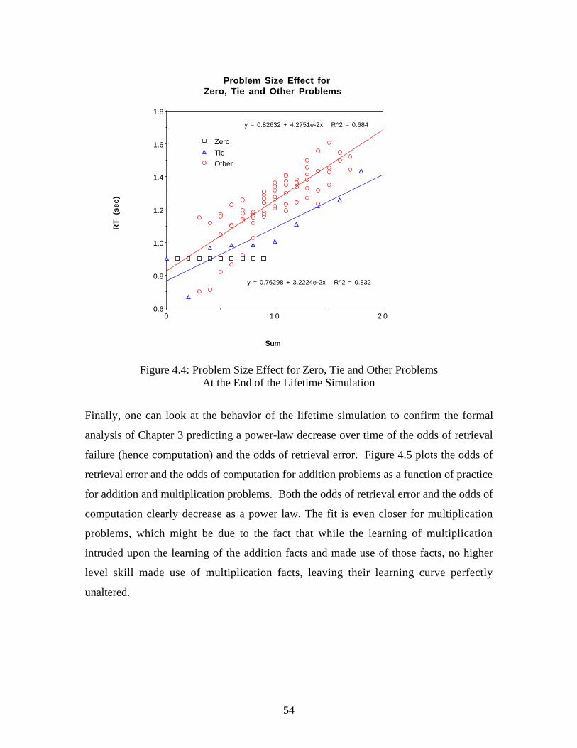
54

2 01 000.6

0.8

1.0

1.2

1.4

1.6

1.8

Zero

Tie

Other

Problem Size Effect forZero, Tie and Other Problems

Sum

RT

(s

ec)

y = 0.76298 + 3.2224e-2x R^2 = 0.832

y = 0.82632 + 4.2751e-2x R^2 = 0.684

Figure 4.4: Problem Size Effect for Zero, Tie and Other ProblemsAt the End of the Lifetime Simulation

Finally, one can look at the behavior of the lifetime simulation to confirm the formal

analysis of Chapter 3 predicting a power-law decrease over time of the odds of retrieval

failure (hence computation) and the odds of retrieval error. Figure 4.5 plots the odds of

retrieval error and the odds of computation for addition problems as a function of practice

for addition and multiplication problems. Both the odds of retrieval error and the odds of

computation clearly decrease as a power law. The fit is even closer for multiplication

problems, which might be due to the fact that while the learning of multiplication

intruded upon the learning of the addition facts and made use of those facts, no higher

level skill made use of multiplication facts, leaving their learning curve perfectly

unaltered.

55

3210-8

-6

-4

-2

0

2

4

Retrieval Errors

Computation

Odds of Retrieval Error and Computation forAddition Problems as a Function of Practice

Log Cycle

Log

Odd

s y = - 0.68179 - 1.3577x R^2 = 0.954

y = 2.1822 - 4.2343x R^2 = 0.979

3210-8

-6

-4

-2

0

2

4

Retrieval Errors

Computation

Odds of Retrieval Error and Computation forMultiplication Problems as a Function of Practice

Log Cycle

Log

Odd

s

y = - 5.2427e-2 - 1.8697x R^2 = 0.976

y = 3.7187 - 4.8421x R^2 = 0.999

Figure 4.5: Odds of Retrieval Error and of Computationas a Function of Practice: (a) Addition; (b) Multiplication

56

In addition to the data fits previously reported, these computation and retrieval error

curves generally fit the data reported by Siegler & Robinson (1982), Siegler & Shrager

(1984) and Siegler (1988) on the percentage of strategy use and retrieval errors at various

points of development. Together, these results, and a few more presented in later

chapters, provide a strong corroboration of this model and ACT-R’s theory of learning.

4.3 Associative Strengths and Interference

4.3.1 General Introduction

In the Posterior Strength Equation, the empirical value, weighted by the number of

observations F(Cj), will come to dominate the prior, weighted by the constant parameter

assoc 17, and the Rji ratio will converge to the empirical ratio Eji:

EF N C F C

F N F

F N C F

F N F Cjii j j

i

i j

i j

= =⋅

⋅( & ) ( )

( )

( & )

( ) ( )

where F(Ni&Cj) is the number of times that i was needed when j was in the context, F(Cj)

is the number of times that j was in the context, F(Ni) is the number of times that i was

needed and F is the number of production firings since i was created.

In this domain, j is usually a number or arithmetic operator and i is an arithmetic (or

counting) fact.18 If the number j is usually not in the context when i is needed, then the

empirical ratio will be very small since F(Ni&Cj) will be much smaller than F(Ni), and

the associative strength Sji, which is equal to the logarithm of the ratio Rji, will be very

negative. This seems a bit surprising since the Prior Strength Equation specifies that

17 The Associative Learning (:al) global parameter, set to 1.0.18 This pattern of associative strengths running from basic components of the domain tochunk representing small groups of these components is general enough to suggest adichotomy in declarative memory between basic referable elements and higher-order

57

unconnected chunks should have an initial strength of 0. However, that is merely a

convenient simplification. In the case of connected chunks (i.e. j appears in a slot of i),

the value of F(Ni|Cj) is assumed to be 1/n, where n is the number of chunks connected to

j. That means that the total probability of retrieving a chunk connected to j is 1, which

implies that the probability of retrieving a chunk unconnected to j is 0. Since the prior

strength of association is the logarithm of the ratio of that probability over the base

probability, if the Prior Strength Equation were consistent that would mean that the prior

strength between unconnected chunks should be minus infinity instead of 0. However,

that would immediately preclude the retrieval of any chunk when an unconnected chunk

is in the context, a somewhat extreme situation. However, given the proper training, the

Posterior Strength Equation indeed specifies that those values will become increasingly

and unboundedly negative.

If one makes the opposite assumption that the number j is always in the context when i is

needed (e.g. 4 is always in the goal when 3+4=7 is retrieved), then the empirical ratio will

tend to F/F(Cj), which will be stable over time if numbers are presented fairly uniformly.

Interestingly, if one assumes that all chunks were created at about the same time (an

assumption that is only approximately true for arithmetic chunks but that becomes

increasingly true as time passes), then F, the number of production firings since the

creation of the chunk, simplifies away and the strength of association from a chunk j

becomes inversely proportional to F(Cj), its frequency of appearance in context. In this

case, that means that larger numbers, which appear less often, will spread more activation

to their connected chunks than smaller numbers do.

This will tend to mitigate the effect of frequencies upon base-level strength, but only

partially. To see that, let us assume that the frequencies of facts in the addition table

decreases linearly with each operand, and consider the extreme chunks in the table: 0+0

and 9+9. If 0+0 is 3 times more frequent than 9+9, then according to the approximate

form of the Base-Level Learning Equation, the difference between the base-level

activation of 0+0 and 9+9 is the logarithm of their frequency ratio, i.e. ln(3). However,

non-referable chunks.

58

because 0 appears as a source for chunks that are less frequent than 0+0 and 9 appears as

a source for chunks that are more frequent than 9+9 (e.g. 0+9 features both and is twice

as frequent as 9+9), then the average frequency of 0 being a source is only 2/3 higher

than the average frequency of 9 being a source. In other words, the frequency distribution

of chunks is always more extreme than the aggregate distribution of their components. In

this case, the difference between their sources of activation is only ln(1.6), which is

significantly less than the difference in base-level activation. This effect of frequency

upon strengths of association is also reduced because all addition chunks have one source

in common, i.e. the operator +, leaving only 2/3 of the total source level to be frequency-

sensitive. Of course, a value of W higher than 1 will tend to amplify this effect of

strengths of activation, but presumably not to the point where it would overwhelm the

primary frequency effect on base-level activation.

This effect is somewhat surprising and is in fact a variant of the fan effect (e.g. Anderson

& Reder, in press), that states that the activation spread from a source to related chunks

will decrease with the number of related chunks. In this case, the activation spread

decreases with the number of appearances of the source in the context, irrespectively of

how many chunks it is connected to. In any case, it is a good thing that the effect of

frequency on the base-level strength predominates since if the strengths of association

did, then ACT-R would predict that chunks that are retrieved more often are actually less

active and take longer to retrieve than chunks that are retrieved less often, a clearly

undesirable result. Indeed, this inversion of the problem size effect sometimes appears

for pathological parameter values, as will be demonstrated in Chapter 5.

A more serious problem results from the fact that the Prior Strength and Posterior

Strength Equations, which specify the default and learned values of the associative

strengths respectively, take into account every appearance of a chunk in the context,

independently of the type of the retrieved chunk or the slot in which it appears. This

assumption can lead to some counterintuitive results involving interference among facts:

between operands of arithmetic facts, between operands and result of arithmetic facts,

between arithmetic and counting facts, and within counting facts. The latter is actually

59

used to produce counting errors to addition problems, though it could be argued that the

pattern produced is excessively geared toward one particular error (“x is followed by x”)

at the exclusion of all other, perhaps more plausible ones. These interference problems

will be examined in detail, the practical solutions adopted in the simulation will be

reviewed, and a possible change in the architecture to address the root of the problem will

be discussed.

4.3.2 Tie Problems

As described in the previous section, two different kinds of strengths of association will

result from the associative learning mechanism applied to an arithmetic problem such as

3+4=?. Positive strengths will emerge from the components of the problem (3, + and 4 in

this case) to the problem chunk itself, as well as other chunks containing some of the

same components (e.g. 3+5=8). Because those strengths converge to the empirical part

of the Posterior Strength Equation, which is essentially the logarithm of a frequency ratio,

their absolute value will be strongly limited (e.g. seldom higher than 2 or 3). The second

type of strengths will occur between the components of the problems and chunks in

which they do not appear (e.g. between 4 and 3+5=8). Those strengths will be initialized

to 0 by the Prior Strength Equation (actually, for computational reasons the link is

omitted altogether, which is equivalent), but once those chunks have been retrieved with

that source in the context (e.g. 3+5=8 being mistakenly retrieved for the problem 3+4=?),

a new link is created and associative learning now applies. Since retrieving that fact with

that source in the context is quite rare, the resulting frequency ratio is very small, and the

logarithm transformation will yield an unboundedly negative strength of association.

Unlike the first type of strength which primed (i.e. raised the activation of) the chunks

likely to be useful, this second type of strength will inhibit the retrieval chunks which

have been a source of errors in the past. Both types of strengths of association are useful,

but the latter, inhibitory type is essential in reaching a near-perfect performance in the

presence of noise and partial matching, because its magnitude can grow unboundedly

large very quickly due to its logarithm form.

60

Tie problems (e.g. 7+7=?) are unusual with respect to both types of strengths of

association. As was previously mentioned, because the operand is repeated twice in the

statement of the problem, its strength of association is higher. When comparing the

strengths of association from a number (e.g. 7) to its tie problem (i.e. 7+7=?) and a non-

tie-problem (e.g. 7+8=?) of similar frequency and creation time, one can see that of the

quantities used in computing the empirical ratio, all are about equal19 except for the co-

occurrence statistics F(Ni&Cj). These are twice as large for the tie problem because the

number appears twice in context, and thus results in two co-references instead of one.

Thus the strength of association to a tie problem from its operand is higher than the

strength of association to other similar problems by an amount of ln(2). This factor is

also reflected in the initialization of the strengths of association using the Prior Strength

Equation. In the static simulations presented previously, this explained why tie problems

were retrieved faster and more reliably than other problems of similar magnitude.

Tie problems are also remarkable when it comes to inhibitory connections. Other, non-

tie problems (e.g. 7+8=?) have different operands and thus two number sources, thereby

inhibiting other problems, including those on the same row (e.g. 7+9=? is inhibited by 8)

or column (e.g. 6+8=? is inhibited by 7) of the addition table. Tie problems, on the other

hand, have only one operand repeated twice and thus cannot inhibit problems on the same

row or column of the addition table. The reason is that other facts (e.g. 7+8=15) are

correctly retrieved quite often with their own components as sources (i.e. 7, + and 8), and

thus will develop positive rather than negative associations from those sources. The tie

problems in the same row or column of the table (e.g. 7+7=?) have as sources of

activation a subset of the sources for those non-tie problems (i.e. 7 and +), and thus

cannot inhibit those problems.

The result is a basic asymmetry between commission errors for non-tie- vs. tie-problems.

Non-tie problems (e.g. 7+8=?) develop inhibitory connections to other facts, including tie

19 F(Cj) are equal because they refer to the same source, F(Ni) are about equal becausethey are of similar frequency, and F are about equal because their creation times aresimilar

61

facts involving those operands. These connections, as they become increasingly

negative, prevent those facts (e.g. 7+7=14) from being mismatched to that problem

because the negative activation they receive becomes too much to overcome consistently

with factors such as noise. Tie problems, however, cannot develop inhibitory

connections to facts in the same table row or column, because those facts include as

sources of activation a superset of the tie problem’s sources. Therefore, even though

those tie facts benefit from a small constant factor of activation boost due to the source

redundancy, that is not enough to consistently overcome noise and other confusion

factors. The result is that while non-tie problems asymptote toward perfect performance,

tie-problems never do and even ultimately get worse as non-tie problems gradually get

stronger. This is clearly an undesirable result. It should be emphasized that this is a

direct result of the assumption that strengths of association from a source of activation to

a chunk reflect the statistics of retrieval of that chunk given that that source is in the

context, and are independent of where that source appears in the chunk if it appears at all.

A version of this assumption is known in the field of machine learning as the Naïve

Bayes Assumption (Mitchell, 1997), which states that the attribute values (sources of

activation) are conditionally independent given the target value (chunk retrieved). It

provides for a sometimes-enormous computational simplification and has been quite

successful in practical applications, and indeed in past ACT-R models. However, the

limits of this assumption have been exposed by the lifetime simulation because of the

fundamental dependency on the learning mechanisms.

There are a number of possible solutions. An easy one would be to simply increase the

Associative Learning global parameter, which controls the weight given to the prior term

in the associative learning formula. This would delay the effects of the empirical ratio,

including the increase in tie errors but also the emergence of strong inhibitory

connections, and thus the asymptote to perfect performance for other problems. It might

provide some quantitative improvement, but simply shifts the learning curve while

leaving the basic problem intact. One might also argue that tie problems occur more

often than others do (e.g. Ashcraft, 1992). While this might be true and would certainly

help, it would only raise the base level and strengths of association to tie facts by a

62

constant factor, and like the basic ln(2) effect of source duplication would not affect the

long-term effect of associative learning, simply delaying it.

The solution that was adopted, as described in the first section of this chapter, consisted

in explicitly recoding tie problems. When a tie problem is encountered, before a solution

is attempted, the repeated argument is replaced by the special chunk Double, to represent

the fact that this argument is identical to the previous one. This explicit re-encoding is

consistent with ACT-R’s theory of chunk creation (see Anderson & Lebiere, 1998, pp.

23-24) because whereas chunks that result from the direct encoding of objects in the

environment (e.g. 3 is the first digit) are automatically produced by the perceptual

interface, chunks that originate as goals (e.g. 3+4=7) are the result of explicit processing,

including the serial gathering of a number of perceptual chunks. It is therefore natural

that some regularities, in this case the repeating of arguments, be detected during the

building of the goal chunk from perceptual chunks, and the result of this detection

encoded in the goal chunk. This is consistent with the findings of Eliaser, Siegler,

Campbell & Lemaire (in preparation) that subjects spend more time encoding tie

problems than regular problems. This additional time could represent the time to fire the

production that detects the argument duplication. Eliaser et al. also found that non-tie

problems exhibit better performance than tie problems in artificial problem sets where tie

problems are the rule rather than the exception as they are in arithmetic. This suggests

that the advantage enjoyed by tie problems in arithmetic in not intrinsic but instead a

matter of explicit representation.

This recoding removes the duplication in the context of tie problems and provides them

with a source of activation distinct from non-tie problems, i.e. the chunk Double. That

chunk will develop a positive associative strength to tie problems and a strongly negative

associative strength to non-tie problems because it does not appear in their formulation.

This exactly provides the contextual discrimination lacking in the straightforward

representation. Also, the chunk Double appears as argument in arithmetic facts about

half as often as numbers do. For example, it will appear in 10 (correct) single-digit

addition facts (corresponding to all the tie problems) whereas a number (e.g. 7) will

63

appear as argument in 19 (10 as first argument and 10 as second argument, with the tie

problem counting twice). Therefore, the positive strength of association from the chunk

Double to tie problems will be about ln(2) higher in average than the strength of

association from a number to a problem involving it as argument. This provides to tie

problems the same advantage in associative strength that a double source did, but this

time it results from an explicit recoding strategy rather than from an architectural feature.

4.3.3 Near-tie Problems

A related problem concerns what can be called near-tie problems, i.e. problems such as

6+7 that are located near the diagonal in the addition table. The main problem results

from argument confusion, i.e. when presented with the problem 6+7=? the model often

retrieves 7+6=13 instead, because that chunk has similar base level activation and

associative strengths, and the mismatch penalties (for matching 7 for 6 and vice versa)

are fairly small. Since addition (and multiplication) is commutative, that results in a

correct answer. The problem is that as one gets away from the diagonal (e.g. 6+8, 6+9,

5+9, etc), this beneficial confusion effect decreases rapidly with the difference between

arguments because the mismatch penalty that applies to each argument becomes too large

to overcome. For example, for 9+4=13 to match to 4+9=? would require overcoming

twice the dissimilarity between 4 and 9 which is much larger than between 6 and 7.

Those problems could potentially mismatch to a close fact which also yields the right

answer (i.e. 5+8=13 for 4+9=?), but the likelihood of that is very small because that fact

will receive no positive spreading activation, and as learning proceeds much negative

activation.

The result is that problems near the diagonal (e.g. 6+7=?) will tend to have lower error

rates than problems of equal size and frequency further away from it (e.g. 4+9=?), a

pattern that is not supported by data. This effect is particularly noticeable for large

problems, whose numbers are more similar to each other (e.g. 6+7=? vs. 3+4=? because 6

is more similar to 7 than 3 to 4), and toward the end of the switch to retrieval, when those

problems develop distinctive associative strengths.

64

A minor additional contributor to the problem is the solution to the previous problem.

Since tie facts are represented with the double chunk, they are very unlikely to intrude

upon non-tie facts (e.g. 6+Double=12 will not mismatch often to 6+7=? because Double

is not similar to 7), and thus problems near the diagonal lose some of their closest

intruders, which also lowers their error rates. However, this contribution is small and the

main effect originates from the associative strengths, in particular the fact that the

strengths are not slot-specific. Thus the chunk 7+6=13 will receive the same associative

strength as the chunk 6+7=13, even though the sources appear in the chunk in the reverse

order in which they appear in the retrieval template 6+7=?. There is no clear solution to

this problem.

4.4.4 Corner Problems

The previous sections dealt with the interference effects of associative strengths from the

problem arguments. The slot holding the result can also produce undesirable interference

effects through associative strengths. As in the previous section, those effects are most

noticeable when the values interfering with each other, in this case the result and one of

the operands, are very similar. That means problems in the top right and bottom left

corners of the addition table, in particular problems of the form 1+x=? or x+1=? for large

values of x (e.g. 1+7=8) because their similarities are less differentiated. In those

problems, the large argument (e.g. 8 in 1+8=?) will prime not only the correct fact (i.e.

1+8=9) but also an incorrect fact (1+7=8) because that argument appears as the result.

Since the mismatch penalty between large close numbers (e.g. 7 and 8) is small, this will

result in an unusually large percentage of errors for those problems, which the data

doesn’t display.

One solution is to make sure that the associative link from a number (e.g. 8) to an

addition fact mentioning it as result (i.e. 1+7=8) is not reinforced. Even though a link is

created by the Prior Strength Equation, it will not be reinforced by the usual addition

retrieval because only the operands and operator appear as sources of activation.

65

However, when an arithmetic goal (e.g. 1+7=8) is popped and reinforces an identical

existing chunk, the associative strengths from the arguments to that chunk must be

reinforced because otherwise they will keep decaying and the chunk will never be

retrieved. The solution is to have ACT-R reinforce upon merging the strengths of

association from the sources of activation when the goal was created (i.e. the operands

and operator), but not from the result slot value, which was filled afterward.

There are essentially two justifications for this reinforcement rule. The first is in the

basic understanding of learning as improving performance in similar situations. Thus

when a chunk is retrieved, the base-level activation of that chunk is reinforced, as are the

strengths of association from the context chunks, all of which will improve the retrieval

performance in the same context. In the case of goal merging, the similar situation is

when an identical goal is created again. Ideally, that goal could be completed directly by

retrieval of a past instance of that goal, instead of having to resort to less efficient means

such as pushing subgoals to compute the answer. Thus the proper quantities to reinforce

when a goal is popped are its base-level activation, and the strengths of association from

the context chunks when that goal was created, because that is when retrieval will be

needed in a subsequent episode. Reinforcing the strength of association from the result

can only result in the kind of interference described at the start of this section.

The second justification arises from the nature of the sources of activation. In the current

ACT-R, a chunk becomes a source of activation instantly when it becomes part of the

goal, and ceases to be a slot value just as immediately when it stops being part of the

goal. Lovett, Reder, & Lebiere (in press) have argued that a more realistic model would

have the sources of activation gradually accruing strength over time when they are part of

the goal, with that strength decaying exponentially when they are not. Under this model,

the operands and operator, which are part of the goal since its creation, will be much

stronger sources of activation than the result, which only became part of the goal just

before it is popped. Thus the reinforcement of the strengths of association when the goal

is popped would reflect that differential source level and result in much higher strengths

from operands and operator than from the result. This theory of source-level

66

accumulation might also explain the need for unequal source levels noted by Anderson &

Reder (in press).

4.3.5 Cross-type Interference

One illustration of the undesirable effects of the type-independence assumption of

associative strengths is the pattern of interference between arithmetic and counting facts.

Since the vast majority (and the entirety of those modeled here) of arithmetic retrievals

involves single-digit operands, the process of arithmetic retrieval creates associative

interference primarily from single-digit numbers. In tasks such as addition by repeated

counting, however, counting facts are retrieved for double-digit as well as single-digit

numbers. This means that the pattern of errors (and latency) for counting will display a

strange discontinuity: a higher percentage of errors for single-digit counting facts due to

the associative interference from arithmetic facts, dropping suddenly when counting

above 10.

This pattern is of course not unavoidable and could in fact be masked by many other

factors. For example, it might be that the single-digit counting facts are practiced and

rehearsed, independently of their use in addition, much more often than the double-digit

counting facts. That additional practice might compensate or even overwhelm the larger

interference effect for single-digit facts. Or the interference effect from arithmetic

retrieval for double-digit numbers might be understated. For example, retrieving those

same arithmetic facts for subtraction or division purposes would entail having in the

context the result as well as one of the operands, which would lead to associative

interference for the result value which of course can be a double-digit number even for

single-digit operands. Another possibility would be that the frequency discontinuity for

arithmetic facts is artificial, either because the frequency of use of the largest single-digit

facts (e.g. 9+5) is very low or because the frequency of the double-digit facts (e.g. 11+3)

is higher, or both. Any of these factors, or possibly some combination of them, would

obscure this particular pattern. But the fundamental problem of the improbability and

undesirability of facts of very different types significantly interfering with each other

67

remains. There is no obvious solution to this specific problem.

4.3.6 A More General Solution

It appears that the pattern of interference resulting from associative priming to a slot other

than the one intended in the matching (e.g. 8 activates 1+7=8 even though one is looking

for a chunk matching 1+8=?) is generally undesirable, as is the interference resulting

from the statistical patterns of use of other chunk types (e.g. limiting addition facts to

single digits makes counting up single digits harder than counting up double digits).

What seems to be needed is a way to make associative connections slot- and type-

specific.

One could make the frequency statistics used in the empirical ratio specific in that way,

but the record-keeping then becomes very onerous and the statistics less reliable because

separate values have to be kept for each type and slot.20 It also leads to occasionally

counterintuitive predictions, for example that, assuming equal fans, the prior strength of

association (as determined by the Prior Strength Equation) to a chunk of a certain type

would be larger than the prior strength of association to a chunk of another type if there

were more elements of the former type. That seems clearly undesirable: all things being

equal, more chunks of a certain type ought to mean more interference, and thus worse

performance, not the better performance resulting from stronger strengths of associations.

More generally, maintaining slot- and type-specific connections seems generally

unworkable. For example, the same number (e.g. 7) could develop both a positive

strength of association to a chunk (e.g. 7+8=?) because it appears as a slot value (i.e. the

first operand) when the chunk is retrieved but also a negative strength of association

because the chunk is occasionally mismatched when it appears in another slot (e.g. 7+7=?

where it appears as the second operand). Thus the sources of activation would not be

chunks but chunk-slot combinations. In addition to the increased computational expense

20 These are the same reasons for why the Naïve Bayes Assumption is so popular in

68

of keeping those additional links, this is clearly at odds with the current concept of

strengths of association between chunks, and would lead to a very odd implementation.

A more elegant solution might be to consider the duality between the processes of

activation spreading and partial matching. For example, given a retrieval from the goal

pattern of 3+4=?, the activation spreading will raise the activation of chunks that match

that pattern (contain the sources), and the partial matching will lower the activation of

chunks that mismatch the pattern. Clearly the two mechanisms are performing related

functions and could potentially be unified. One interesting difference is that while

activation is spread to all the chunks to which the source is connected, the partial

matching is type-specific (because only chunks of the right type are allowed to match)

and slot-specific (the desired slot value is matched against the actual chunk slot value,

independently of the other sources appearing in the other slots). This is precisely the

solution to the problems with the strengths of association described in the previous

sections. Could the solution be simply to remove the activation spreading and rely on

partial matching to provide context-specificity?

This would certainly be compatible with ACT-RN (Lebiere & Anderson, 1993), an

earlier implementation of ACT-R using standard neural network constructs, which has

guided the development of ACT-R including the partial matching mechanism (Lebiere,

Anderson, & Reder, 1994). In ACT-RN, the concepts of strengths of association and

partial matching are not separate. The pattern of connections to a chunk from its slots

encode both the association from slot value to chunk, and the distributed pattern of

activation of the slot value which allows different but similar values to capture part of the

strength of association.

One function of the associative learning mechanism which cannot be readily performed

by the partial matching is the gradual discrimination between associative strengths that

occurs over time and leads to increasingly negative strengths of association which result

in near-perfect performance. What could change over time that would allow the partial

machine learning.

69

matching mechanism to initially produce the error-prone performance of children and

later improve to the near-flawless performance of adults? One possibility would be the

similarity values. Smaller, more frequently encountered, numbers are usually considered

less similar than larger, less common numbers (Whalen, 1996). While the better

discriminability between small numbers could be due to their magnitude itself (i.e. two

apples look more different from three than seven from eight), it could also be attributed to

their higher frequency. The ability to discriminate through similarity values between

related concepts might be acquired through practice. This might explain the improved

performance over time as similarity values are increasingly refined and differentiated and

errors of commission are gradually reduced.

Another, perhaps more promising possibility would be the activation noise. ACT-R’s

assumption of an activation noise of constant amplitude is at odds with the intuition that

strong, well-established chunks ought to be less noisy than new, poorly rehearsed

chunks.21 If the amplitude of the activation noise was specific to a chunk and decreased

with the amount of practice of that chunk, then the commission errors involving that

chunk would decrease along with the noise since one term would ultimately come to

dominate the Boltzmann equation as temperature goes down to 0. If one interprets the

decay of base-level activation as being a stochastic phenomenon, this decrease of noise

with practice would explain how decay becomes increasingly slow with practice. One

possible function expressing the noise Sn as a function of practice n and the initial noise S

is:

SS

nn =+1 ln( )

Noise Reduction Equation

Let us assume for simplicity that chunks C1 and C2 are competing for retrieval and that

21 ACT-R 4.0 introduced a Permanent Activation Noise sampled once at the creation ofthe chunk, which is distinct from the Activation Noise added to the chunk activation ateach production cycle and usually of larger amplitude to provide greater initialrandomness. This however would not be helpful in this model.

70

they have had a similar number of retrievals n, then the odds of retrieving chunk C1 are:

Odds C eA A

Sn( )1

1 2

=−

If one expressed the noise level as a function of practice, the odds of retrieval become:

Odds C e e nn A A

SA A

SA A

S( )ln( )

1

1 1 2 1 2 1 2= = ⋅

+( ) −( ) − −

This establishes that if one assumes that the noise level decreases as an inverse function

of the logarithm of practice, then the odds of retrieval (i.e. error) follow a power law of

practice, with the exponent being the ratio of the activation difference between the

competing chunks, divided the amplitude of the initial noise. The speed of convergence

will of course improve with lower noise, but also with wider activation separation

between chunks. This activation difference can result from a difference in frequency of

practice or rehearsal between chunks, as well as from activation penalties resulting from

chunk(s) mismatches. A higher mismatch penalty will therefore also lead to faster

convergence.

Decreasing the noise of chunks over time with their amount of practice is closely related

to the technique of simulated annealing in Boltzmann machines (Ackley, Hinton, &

Sejnowski, 1985; Hinton & Sejnowski, 1986), since noise in ACT-R has an effect similar

to temperature in Boltzmann machines, through the same Boltzmann equation. However,

there are differences as well. The Boltzmann distribution in ACT-R is merely

descriptive, whereas it is also used in Boltzmann machines to control every local unit

fluctuation. More fundamentally, simulated annealing in Boltzmann machines happens

on a small time scale, for every pattern presentation, whereas it would be under this

proposal a long-term process, with the activation noise decreasing over a long time scale

with each rehearsal. Finally, temperature in Boltzmann machines is a quantity global to

the entire network, whereas every chunk in ACT-R would have a different noise as a

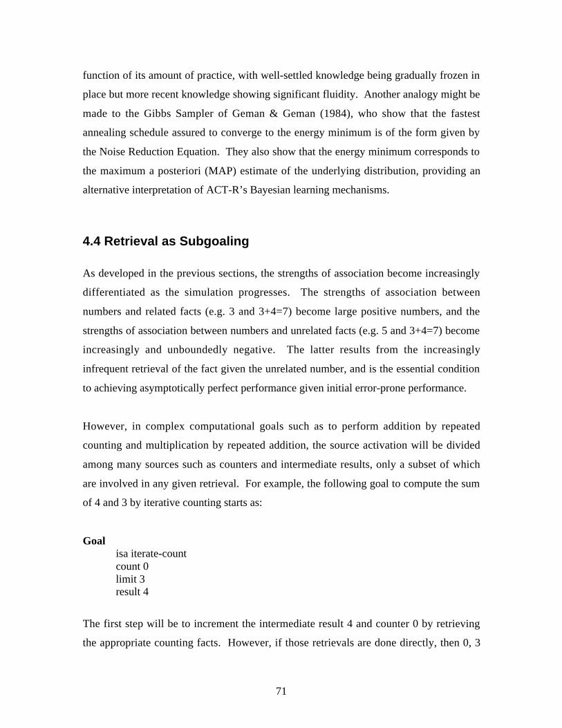
71

function of its amount of practice, with well-settled knowledge being gradually frozen in

place but more recent knowledge showing significant fluidity. Another analogy might be

made to the Gibbs Sampler of Geman & Geman (1984), who show that the fastest

annealing schedule assured to converge to the energy minimum is of the form given by

the Noise Reduction Equation. They also show that the energy minimum corresponds to

the maximum a posteriori (MAP) estimate of the underlying distribution, providing an

alternative interpretation of ACT-R’s Bayesian learning mechanisms.

4.4 Retrieval as Subgoaling

As developed in the previous sections, the strengths of association become increasingly

differentiated as the simulation progresses. The strengths of association between

numbers and related facts (e.g. 3 and 3+4=7) become large positive numbers, and the

strengths of association between numbers and unrelated facts (e.g. 5 and 3+4=7) become

increasingly and unboundedly negative. The latter results from the increasingly

infrequent retrieval of the fact given the unrelated number, and is the essential condition

to achieving asymptotically perfect performance given initial error-prone performance.

However, in complex computational goals such as to perform addition by repeated

counting and multiplication by repeated addition, the source activation will be divided

among many sources such as counters and intermediate results, only a subset of which

are involved in any given retrieval. For example, the following goal to compute the sum

of 4 and 3 by iterative counting starts as:

Goalisa iterate-countcount 0limit 3result 4

The first step will be to increment the intermediate result 4 and counter 0 by retrieving

the appropriate counting facts. However, if those retrievals are done directly, then 0, 3

72

and 4 will all be sources when the counting facts 0->1 and 4->5 are retrieved. The

strengths of associations between those numbers and facts will all be reinforced,

including incidental ones such as between 4 and 0->1, and 3 and 4->5. This would have

two undesirable consequences. The first is interference errors, such as retrieving 3->4

instead of 4->5 because the extra spreading activation from the source 3 overcomes the

mismatch penalty between 3 and 4. While the errors produced by this type of

interference do occur, in this case the interference leads to an excessively deterministic

pattern of errors. An even more fundamental problem is that because of these accidental

reinforcements between unrelated facts and numbers, the strengths of association

between them will not become increasingly negative but instead settle at some base value

that reflects these accidental co-occurrences and that will prevent further improvement in

performance.

The solution is to subgoal retrievals instead of performing them directly. This

corresponds to moving the retrievals from the left-hand side of productions to the right-

hand side and pushing subgoals to perform them on the stack. This operation focuses on

the retrieval to be performed by creating a new goal of the same type as the chunk to be

retrieved and which only includes the activation sources necessary to the retrieval.

Examples of this technique can be found in productions Iterate-Count (which subgoals a

count) and Iterate-Add (which subgoals a number of operations). Once the retrieval

patterns have been subgoaled, a production must fire to perform the actual retrieval,

complete the pattern, and pop the goal. These productions are Count-Up and

Arithmetic-Retrieval for counting and arithmetic facts, respectively. These productions,

which complete a goal by matching it to a chunk in memory, are very basic and can be

found in many other models (e.g. Lebiere & Wallach (in preparation)). Indeed, these

productions are so basic and pervasive that it could be argued that they correspond to an

architectural primitive similar to the Obligatory Retrieval Assumption of Logan (1988).

This technique, in addition to allowing the strengths of association to achieve optimal

predictiveness, has the advantage of increasing the modularity of knowledge. Instead of

having to generate separate productions for retrieval and backup computation in each

73

situation in which an arithmetic fact would be needed, a single production would be

needed to set up a subgoal of that type, which could be solved by either retrieval or

backup computation without the need to duplicate those productions. By pushing a

subgoal that will become a declarative memory chunk when it is popped, it also creates a

permanent record of the retrieval in memory which allows the system to reflect upon its

own problem-solving. It would also improve retrieval performance, because the entire

source level W would be devoted to sources useful to retrieval, and thus would speed up

learning as well by limiting errors.

Finally, it would make for a much simpler implementation of ACT-RN (Lebiere &

Anderson, 1993). In ACT-RN, productions perform retrievals by gating the right

connections between central memory, in which the current goal is held, and declarative

memory, which is implemented as a set of type memories, each of which holding chunks

of a different type. Because any goal can perform any retrieval, the mapping between

goal values and retrieval pattern is arbitrary. Thus productions must have gating

connections to enable any possible permutation from central memory to any type

memory. Because declarative memory is potentially quite vast, this generality is very

computationally expensive. This proposal offers a much more manageable solution.

Because a retrieval is accomplished by first creating a new subgoal, that transformation

can be performed by local connections within central memory. Since the new subgoal

directly specifies the retrieval pattern, the actual retrieval can then be performed by

directly broadcasting the subgoal to declarative memory, without the need for any gating

connection to specify the retrieval pattern or the right type memory. Since retrieval

latency is inversely proportional to degree of match, the type memory holding the chunk

that best matches the subgoal will complete retrieval first and preempt the other

memories in returning the resulting chunk to central memory. This broadcast

communication between the central controller executive and the declarative memory

modules is similar to the CAP2 connectionist control architecture (Schneider & Oliver,

1991; Schneider & Pimm-Smith, 1997).

74

Chapter 5: Parameter Sensitivity

5.1 Introduction

The simulations described here are controlled by a number of real-valued parameters.

The values of those parameters were selected (optimized would imply more precision and

systematicity than could be practically used considering the length of the simulation) to

maximize the fit to the experimental data. A common criticism of ACT-R is that it

contains too many parameters that can be used to tune every aspect of the system.22

While factually correct, this critique mischaracterizes the impact that those parameters

have upon the predictions of a particular model. Clearly some amount of

parameterization is needed in any architecture to account for individual and experimental

variations, estimation of unknown variables (previous knowledge, etc) and the like.

While varying parameter values within a reasonable range will result in different

quantitative predictions, the model’s qualitative predictions are left unaltered. For

example, if one assumes a differential in frequency between small and large facts, any

reasonable ACT-R model will yield a problem-size effect. This is a basic prediction of

the architecture’s learning mechanism.

Moreover, there has been recently a concerted effort (Anderson & Lebiere, 1998) to

understand the effect and constrain the values of ACT-R’s global parameters, i.e. those

parameters that are specified in the architecture and apply to every model. Some

parameters, such as the noise level, have become increasingly constrained to a narrow

range of values. Others, such as the base level decay, have essentially been fixed. Even

those parameters whose values vary more widely, such as the retrieval threshold and

latency factor, can be related to each other through known principles such as the speed-

accuracy tradeoff (Anderson, Bothell, Lebiere, & Matessa, 1998), thereby removing

22 Strangely enough, those critics are often unperturbed by connectionist models, whichby definition consist of little else but parameter estimation, automated and otherwise.

75

further degrees of freedom.

This chapter will examine the sensitivity of the model to its parameters, including global

parameters such as the activation noise, retrieval threshold, and mismatch penalty, as well

as domain-specific parameters such as training schedule, problem distribution, and

feedback strategies. Beyond establishing that the model is not excessively sensitive to

any parameter value and that the results obtained qualitatively hold for a wide range of

values, the goal is to explore the concept of optimality of those parameters, not in terms

of fitting the data but in terms of absolute performance. The concept of optimal values

for the simulation-specific parameters is fairly intuitive as well as practical: given a

particular cognitive system (children, ACT-R model, etc), what is the best way to teach it

arithmetic in terms of how fast to present the problems, how much feedback to give, etc.

Those are questions whose answers would be of some use to educators. The concept of

optimal values for the global parameters of the cognitive system is somewhat different.

One would be tempted to say that the optimal noise value is 0 (so everything is precise

and deterministic), the retrieval threshold is minus infinity (so every chunk is perfectly

recalled) and the optimal mismatch penalty is infinity (so every chunk is perfectly

matched and no error occurs). This essentially corresponds to the purely symbolic mode

of execution of ACT-R, but it represents an overly simple view of cognition. Noise is

useful because it promotes adaptation to a constantly changing environment. A retrieval

threshold is useful because it provides a criterion to establish when no suitable memory

can be retrieved and some alternative strategy must be used. Partial matching is useful

because it provides an ability to generalize by retrieving related information when the

exact match does not exist or is not available. But clearly there must be a limit. If the

noise is too high the system is random. If the retrieval threshold is too high, declarative

memory is useless. Too much mismatching and confusion sets in. There arises the

concept of an optimal value for activation noise, retrieval threshold and mismatch

penalty. But of course such a concept would have to be environment-specific.

Stochasticity, thresholding and approximation are more likely to be useful in an

approximate, rapidly changing environment. And conversely, they are less likely to be

76

useful in a domain such as cognitive arithmetic, which, with its immutable set of facts,

puts a high premium on precision. But it would nonetheless be useful to establish that

those attribute of human cognition, which have evolved in a very different environment

than the precise world of mathematics, are still of some use there. The following sections

will illustrate that this is indeed the case, to a surprising extent. Because of the need to

run the lifetime simulation in each study for a range of parameter values, each data point

represents a single simulation run.

5.2 Activation Noise

The formal analysis established that the activation noise is the main parameter controlling

the speed of convergence to correct fact retrieval. Figure 5.1 presents the results from

running the lifetime simulation for a range of activation noise s values from 0.0 to 0.5,

with all other parameters held constant.

0.60.50.40.30.20.10.0.001

.01

.1

1

10

Error Odds @ 3

Error Odds @ 7

Error Odds @ 20

Odds of Retrieval Error as a function of Activation Noise S

Activation Noise S

Odd

s of

Ret

riev

al E

rror

Figure 5.1: Odds of Retrieval Error as a function of Activation Noise S.

77

The results are presented for 2000-problem cycles 3, 7 and 20, corresponding roughly to

second grade, sixth grade and adulthood. The odds of retrieval error are plotted on a log

scale as a function of the activation noise. The results clearly confirm the theoretical

analysis. For values of s of 0.25 or smaller, the odds of error decrease to about 1% or less

by cycle 7 and to a negligible amount by cycle 20. For larger noise values, the error odds

either stabilize, e.g. to about 10% for s = 0.3, or even increase over time, e.g. to worse

than even odds for s = 0.5. The theoretical analysis predicted that the noise threshold for

convergence would be 1 divided by √2 (because commission errors result from the

combined noise of two chunks) times 3 (because the source activation level for each

argument is 1/3), or about 0.236. The actual threshold is slightly higher, around 0.25,

because other factors such as corrective feedback and mismatch penalty also contribute to

reducing the odds of error.

While this would argue for a noise level as low as possible to ensure the fastest

convergence to the correct answer, other factors enter into a measure of optimality. One

is that very low noise levels occasionally lead to some error becoming ingrained and

preventing convergence to perfect performance because the system is not stochastic

enough to escape the problem. A more fundamental factor is the desirability of retrieving

an answer instead of computing it or relying on external help, which can be time-

consuming and error-prone. Figure 5.2 plots the odds of retrieval at cycles 1, 2 and 3 as a

function of the activation noise level. The odds of retrieval increase roughly as an

exponential function of the activation noise, with the slope of the curve gradually

decreasing over time to about even at cycle 3. In the early cycles, when the activation

level of most chunks is below the retrieval threshold, the larger the noise the more likely

a chunk is to be retrieved. Thus a large noise boosts the odds of retrieval and makes it

possible for the model to switch to retrieval earlier, albeit with more errors. This earlier

switch to retrieval will lead to additional reinforcements from the retrieval process itself,

and will in turn result in not only more common but also faster retrievals, as indicated by

Figure 5.3, which plots the retrieval latency for small and large facts at cycle 7. A higher

noise leads to faster retrieval, especially for large facts.

78

0.60.50.40.30.20.10.0.01

.1

1

10

Retrieval Odds @ 1

Retrieval Odds @ 2

Retrieval Odds @ 3

Retrieval Odds as a function of Activation Noise S

Activation Noise S

Ret

riev

al O

dds

Figure 5.2: Odds of Retrieval as a function of Activation Noise S.

0.60.50.40.30.20.10.02

3

4

5

Small Facts

Large Facts

Retrieval Latency as a function of Activation Noise S

Activation Noise S

Ret

riev

al

Late

ncy

(sec

)

Figure 5.3: Retrieval Latency as a function of Activation Noise S.

79

Thus one could say that by some measure the lifetime simulation noise level of 0.25 is

about optimal, in that it provides the earliest and fastest possible arithmetic retrieval

under the constraint of ensuring convergence to the correct answers. And this optimality

criterion is fairly strict. Because odds of retrieval error increase exponentially with the

noise level, a significantly larger noise value will lead to an unacceptably large

proportion of errors that will not be corrected with practice. And because the odds of

retrieval initially decrease as an exponential of the activation noise, a much lower noise

value will lead to a much slower initial shift to retrieval. Unlike the values of the

retrieval threshold which tend to vary more widely, this value of 0.25 for the activation

noise has been used in other simulations (e.g. Lebiere & Wallach, in preparation; West &

Lebiere, in preparation) and has become something of a recommended setting for the

noise level.

5.3 Retrieval Threshold

A priori, it doesn’t appear that the retrieval threshold would have much impact on the

probability of error. Clearly, through the Retrieval Probability Equation the retrieval

threshold directly determines the probability of a chunk being retrieved, i.e. the odds of

retrieval are:

Odds eA

s=−τ

This inverse exponential relation is confirmed by plotting the log odds of retrieval as a

function of retrieval threshold for the first 3 cycles in Figure 5.4. Thus a lower threshold

provides for a much faster initial switch to retrieval. However, a very fast transition to

retrieval is problematic. If some chunks are being consistently retrieved and are building

up strength while other neighboring chunks haven’t yet started being retrieved, there is a

danger of the stronger chunks being misretrieved for the weaker ones, thus getting even

stronger, and increasingly getting locked in as permanent errors in a vicious rich-get-

richer circle. To resist that phenomenon, one needs a gradual and relatively uniform

80

building of base level and associative strengths before retrieval triggers its own dynamic

feedback loop.

-2.0-2.5-3.0-3.5-4.0-4.5-5.0.001

.01

.1

1

10

100

1000

Retrieval Odds @ 1

Retrieval Odds @ 2

Retrieval Odds @ 3

Odds of Retrieval as a function of Retrieval Threshold

Retrieval Threshold

Odd

s of

Ret

riev

al

Figure 5.4: Odds of Retrieval as a function of Retrieval Threshold.

This analysis is confirmed by the empirical results presented in Figure 5.5, which plots

the odds of retrieval error on a log scale as a function of retrieval threshold at cycles 3, 7

and 20. One can observe a sharp exponential degradation in the odds of retrieval error

below a threshold of –3.75, the retrieval threshold used in the lifetime simulation. For a

slightly lower threshold of –4.0, the percentage of errors stabilizes at about 5%, whereas

for even lower thresholds down to –5 the odds of error actually increase over time to even

odds or even much worse. This dynamic is reminiscent of the effects of large activation

noise values.

However, threshold values larger than –3.75 do not yield better performance. The odds

of error again increase exponentially, though at a much slower pace, and ultimately

decrease over time at the same rate as the optimal value, indicating a different problem

81

than for lower values. The reason for the poorer performance of larger threshold values

results from the use of backup computations: since those strategies have a high error rate,

they generate many erroneous facts that will degrade the retrieval performance later on.

The slope of this performance degradation will depend upon the degree of reliance upon

error-prone backup strategies (versus error-free but potentially burdensome strategies

such as asking a teacher or parent), and convergence to error-free performance will only

be delayed rather than prevented. However, this clearly establishes that delaying retrieval

with further practice is not productive, and clearly establishes an optimal value for the

retrieval threshold.

-2.5-3.0-3.5-4.0-4.5-5.0.001

.01

.1

1

10

100

Error Odds @ 20

Error Odds @ 7

Error Odds @ 3

Odds Of Retrieval Error as a function of Retrieval Threshold

Retrieval Threshold

Odd

s of

Ret

riev

al E

rror

s

Figure 5.5: Odds of Retrieval Error as a function of Retrieval Threshold.

In addition to leading to a sharp increase in errors, a very low threshold also leads to a

very strange latency pattern, as shown in Figure 5.6 plotting the retrieval latency for

small and large facts in cycle 7 as a function of retrieval threshold.

82

-3.0-3.5-4.0-4.5-5.00.5

1.0

1.5

2.0

Small Facts @ 7

Large Facts @ 7

Retrieval Latency as a function of Retrieval Threshold

Retrieval Threshold

Ret

riev

al

Late

ncy

(sec

)

Figure 5.6: Retrieval Latency at cycle 7 as a function of Retrieval Threshold.

Whereas for a retrieval threshold larger than –4.0, the expected problem-size effect

between small and large fact retrieval can be observed, for lower thresholds the problem-

size effect gradually becomes inverted. This is a rather complicated consequence of the

increase in associative strength magnitude with number size described in section 4.1,

combined with the rapid emergence of a few very strong facts at very low threshold.

While somewhat obscure and secondary, this effect reinforces the conclusion that while

they might seem attractive very low thresholds can be disastrous in practice. In

conclusion, similarly to the activation noise, a strongly optimal value for the retrieval

threshold exists due to the sharply exponential increase in errors for lower thresholds and

the much slower switch to retrieval and slighter increase in errors for higher thresholds.

5.4 Mismatch Penalty

Since the mismatch penalty scales the difference in activation between the correct fact

83

and potential mismatching competitors, one would expect an exponential decrease in

errors to result from an increasing mismatch penalty. This is confirmed by the empirical

results of Figure 5.7, which plots the odds of retrieval error as a function of the mismatch

penalty parameter at cycles 3, 7 and 20.

1 086420.001

.01

.1

1

10

100

Error Odds @ 3

Error Odds @ 7

Error Odds @ 20

Odds of Retrieval Error as a function of Mismatch Penalty

Mismatch Penalty

Odd

s of

Ret

riev

al E

rror

Figure 5.7: Odds of Retrieval Error as a function of Mismatch Penalty.

A similar pattern as for activation noise and retrieval threshold again emerges, with the

threshold value for mismatch penalty being the default one of 1.5. Slightly lower values

such as 1.0 result in a stable retrieval error percentage of about 10%. Significantly lower

values lead to a very sharp degradation in performance with error rates increasing over

time to catastrophic levels. A much more gradual increase in performance occurs for

mismatch penalty values greater than the threshold, with uniform convergence over time

to perfect performance.

One could conclude that larger mismatch penalties are more desirable, and the exactitude

84

and monotonicity of arithmetic knowledge makes it one of the most propitious domains

for that assumption. True to the emerging pattern, excessive insistence upon exactitude,

however, will also lead to a slower shift to retrieval, as shown by Figure 5.8, which plots

the odds of retrieval for cycles 1 to 3 as a function of the mismatch penalty:

1 01.1.01

.1

1

10

100

Retrieval Odds @ 1

Retrieval Odds @ 2

Retrieval Odds @ 3

Odds of Retrieval as a Function of Mismatch Penalty

Mismatch Penalty

Odd

s of

Ret

riev

al

Figure 5.8: Odds of Retrieval as a function of Mismatch Penalty.

There is to a slight but discernible increase in speed of retrieval with decreasing

mismatch penalties. This results because decreasing mismatch penalties will increase

retrieval errors. However, incorrect retrievals still qualify as rehearsals for the facts to

which they correspond and, at least in the early cycles, the feedback correction gives the

correct fact the same rehearsal that a correct retrieval would have provided. Thus

incorrect retrievals actually lead to more rehearsals and more retrievals. In conclusion,

an optimal value again emerges which provides for the fastest switch to retrieval under

constraint of convergence to the correct answers.

85

5.5 Presentation Schedule

In addition to the architectural parameters examined in the previous section, the behavior

of the lifetime simulation is controlled by a number of parameters specific to the domain

of cognitive arithmetic. One of these is the presentation schedule. While many

variations are possible, the most straightforward manipulation is to vary the average time

delay between problem presentations. One would expect that shorter delays, i.e. a more

intense schedule, would lead to faster and better retrieval, and the former is certainly

correct, as evidenced by Figure 5.9, which plots the odds of retrieval for cycles 1 to 3 as a

function of inter-problem delay:

100000100001 0 0 01 0 0.001

.01

.1

1

10

100

Retrieval Odds @ 1

Retrieval Odds @ 2

Retrieval Odds @ 3

Odds of Retrieval as a function of Inter-Problem Delay

Delay (sec)

Odd

s of

Ret

riev

al

Figure 5.9: Odds of Retrieval as a function of Inter-Problem Delay.

One can see that the odds of retrieval decrease as a power function of the inter-problem

delay with an exponent of about -2. This can be derived by replacing in the approximate

form of the Base-Level Learning Equation the total life of the chunk T with n.l where n is

the number of references and l is the lag or inter-problem delay to obtain:

86

Bn l

d

d d

= ⋅−

− −ln

1

1

This new expression of the base-level activation can then be used in the odds version of

the Retrieval Probability Equation to yield, using C to abstract away the constant

activation terms:

Odds C e C ld l

sd

s= ⋅ = ⋅− −ln

which confirms not only the power-law form of the relation between odds of retrieval and

inter-problem delay, but also the exponent value of about –2, since the base-level decay

exponent d is 0.5 and the activation noise level s is 0.25. Thus a smaller inter-problem

delay, hence a more intense schedule, leads to faster retrievals, but not necessarily better

retrievals, as Figure 5.10, which plots the odds of retrieval error as a function of inter-

problem delay for cycles 3, 7 and 10. Again an optimal value emerges at about 7500

seconds of inter-problem delay, the value used in the lifetime simulation. For shorter

delays, the performance quickly degrades and actually gets worse over time. A slightly

shorter delay of 5000 seconds is initially slightly better but doesn’t seem to converge as

well. Somewhat larger delays up to 25000 seconds are initially slightly worse but

converge as well as the optimal value, but of course they take up to three times as long as

the optimal value since the total time scales linearly with the delay. Even larger delays

start and stabilize at about 10% errors.

The explanation is similar to that for the retrieval threshold, since the main effect of inter-

problem delay is to uniformly raise or lower the base-level activation, which is equivalent

to respectively lowering or raising the retrieval threshold. Very low inter-problem delays

will lead to a quick buildup of base-level activation and thus an early retrieval of chunks,

which results in a catastrophic performance degradation as a few chunks overwhelm the

others in a rich-get-richer grab. Larger inter-problem delays are safer, but result in more

frequent uses of the backup computation procedure, which introduces additional errors.

87

1000000100000100001 0 0 01 0 01 0.001

.01

.1

1

10

100

Error Odds @ 3

Error Odds @ 7

Error Odds @ 20

Odds of Retrieval Error as a function of Inter-Problem Delay

Delay (sec)

Odd

s of

Ret

riev

al E

rror

Figure 5.10: Odds of Retrieval Error as a function of Inter-Problem Delay.

100000100001 0 0 01 0 0.1

1

10

Small Facts @ 7

Large Facts @ 7

Retrieval Latency as a function of Inter-Problem Delay

Delay (sec)

Ret

riev

al

Late

ncy

(sec

)

Figure 5.11: Retrieval Latency as a function of Inter-Problem Delay.

88

Very short inter-problem delays lead to faster retrievals but also, just as for very low

retrieval thresholds, to a pathological inversion of the problem-size effect, as shown in

Figure 5.11, which plots the retrieval latency for small and large facts at cycle 7 as a

function of inter-problem delay:

In conclusion, the pressure to adopt a more intense presentation schedule is strong, since

it leads to much earlier and faster retrievals, but a strong limit is imposed by the

catastrophic performance degradation at very short delays23. The optimal inter-problem

delays of 7500 to 5000 seconds correspond to 4000 to 6000 problems per year

respectively, which is consistent with the textbook frequencies reported by Ashcraft &

Christy (1995).

5.6 Steepness of Frequency Distribution

Another well-studied characteristic of the domain of cognitive arithmetic that is essential

to the present explanation of the problem-size effect is a problem distribution whose

frequency decreases with the problem size. As previously mentioned, a linearly

decreasing probability distribution was assumed and the slope of the probability density

function will be referred to as the steepness of the frequency distribution. That number

can be understood as follows: in a 10x10 table, the average fact will have a probability of

0.01. If the slope is 0.0005 (the number used in the simulation), then the probability of

neighboring facts in the table will differ by that amount. This implies that the most

common fact has a probability of 0.0145 and the least common a probability of 0.0055,

which leads to a frequency ratio between most common and least common facts of about

2.6. Averaging over rows or columns, that also implies that the ratio between most

common and least common argument is about 1.6. This corresponds fairly closely to the

textbook frequencies reported by Ashcraft & Christy (1995) and Hamman & Ashcraft

(1986).

89

One would assume from the omnipresence of the problem-size effect that the steepness of

the frequency distribution would have a significant effect on the performance of the

system. Surprisingly enough this is not quite the case, as is shown by Figure 5.12, which

plots the odds of retrieval error as a function of the steepness of the frequency

distribution for cycles 1, 2, 3, 7 and 20:

0.00100.00080.00060.00040.00020.0000.001

.01

.1

1

Error Odds @ 1

Error Odds @ 2

Error Odds @ 3

Error Odds @ 7

Error Odds @ 20

Odds of Retrieval Error as a function ofthe Steepness of the Frequency Distribution

Steepness of Frequency Distribution

Odd

s of

Ret

riev

al E

rror

Figure 5.12: Odds of Retrieval Error as a function of Steepness of FrequencyDistribution.

During the first three cycles, the odds of retrieval error are fairly insensitive to the

steepness of the distribution. However, for very steep distributions (0.00075 and over,

which correspond to a ratio between most and least common fact of over 4.0), the odds of

error stabilize above 5% and do not improve further, while they converge to fewer than

1% for more even distributions of slopes of 0.0005 or smaller. The data for the perfectly

even distribution is somewhat unrepresentative, in that a single fact developed a

23 This of course is somewhat sensitive to other parameters, such as the amount of

90

consistent error that could not be improved and which accounted for most of the final

error, but it should serve as a reminder of the stochastic nature of the results.

One reason for the absence of a strong effect results from the nature of the distribution

itself. The errors caused by a steep distribution will occur for the least frequent problems

because they are weakest, but since they are the least frequent problems they will also

affect the average error odds the least. Hence the worst of the effect is minimized. But

the main reason is that the effect of a regular problem distribution on the relative

activation of arithmetic chunks, no matter how steep, is actually quite small compared to

the other factors producing variations of activation such as noise, schedule randomness

and other non-regular frequency variations. As previously seen, the difference in the

base-level activation of two chunks of differing frequencies but equal total lives is 0.5

(i.e. 1-d which is usually 0.5) times the logarithm of the ratio between the chunk

frequencies. Even for the extreme slope of 0.001, which presents the most common

problem 19 times more often than the least common one, the average frequency ratio

between neighboring facts is 1.1, which yields a difference in base-level activation of

only about 0.025, which is almost negligible. And because the mismatch penalty sharply

increases with distance, the activation differences between neighboring facts are the ones

that really matter.

The effect of the steepness of the frequency distribution on odds of retrieval is very

limited as well, as Figure 5.13, which plots the odds of retrieval at cycles 1 to 3 as a

function of the steepness of the frequency distribution, demonstrates. The curves are by

and large flat, with a small effect that changes over time. During the first cycle, when the

odds of retrieval are about 0.1, the steeper distributions have somewhat better retrieval,

mainly because their small facts are more frequent than for flatter distributions, and thus

have a higher base-level activation and a better chance of being retrieved. During the

third cycle, when the odds of retrieval are about 10.0, the flatter distributions have better

retrieval, because their large facts are more frequent than for steeper distributions, and

thus are more active and have a better chance of being retrieved. The reasoning of cycle

feedback. In general, the optima discussed here are only local.

91

1 concerning the small facts is not applicable because those facts are not consistently

retrieved independently of the distribution. The second cycle, when the odds of retrieval

are about 1.0, combines the advantages of the first and third cycle, with the middle

distribution having the lowest retrieval. But all those effects are so small as to be

negligible.

0.00100.00080.00060.00040.00020.0000.1

1

10

100

Retrieval Odds @ 1

Retrieval Odds @ 2

Retrieval Odds @ 3

Odds of Retrieval as a function ofthe Steepness of the Frequency Distribution

Steepness of Frequency Distribution

Odd

s of

Ret

riev

al

Figure 5.13: Odds of retrieval as a function of Steepness of Frequency Distribution.

The problem-size effect is of course the measure on which the steepness of the frequency

distribution has a significant effect. Figure 5.14 plots the retrieval latency for small

(single-digit sum) and large (two-digit sum) facts at cycle 7 as a function of the steepness

of the frequency distribution. The problem-size effect is 0 for an even distribution and

increases about linearly with the steepness of the distribution. One can easily prove

through a basic summation argument that the ratio between the sum of the frequencies of

small and large facts grows with the square of the steepness of the frequency distribution

function, as Figure 5.15 shows.

92

0.00100.00080.00060.00040.00020.00001.2

1.4

1.6

1.8

2.0

2.2

2.4

Small Facts @ 7

Large Facts @ 7

Retrieval Latency as a function of theSteepness of the Frequency Distribution

Steepness of Frequency Distribution

Ret

riev

al

Late

ncy

(sec

)

Figure 5.14: Odds of retrieval as a function of Steepness of Frequency Distribution.

0.00100.00080.00060.00040.00020.00001.2

1.4

1.6

1.8

2.0

2.2

2.4

2.6

Frequency Ratio Small/Large

Average Latency

Frequency Ratio between Small and Large Factsand Average Latency as a function of Steepness

Steepness of Distribution Function

Fre

qu

en

cy

Ra

tio/L

ate

ncy

(s

ec)

y = 1.2267 + 695.49x + 5.8171e+5x^2 R^2 = 1.000

Figure 5.15: Effect of Steepness of Frequency Ratio and Average Latency

93

When one expresses the total life of the chunk in terms of the number of references times

a constant lag, as was done in the previous section, one can see that the base-level

activation grows with (the logarithm of) the frequency of that chunk to the power of 1-d,

which given the default value of 0.5 for the base-level decay exponent is 0.5. Thus this

exponent of 0.5 will cancel the square, and the base-level activation will be proportional

to the logarithm of the steepness of the distribution function. Since the retrieval is the

exponential of the activation, the problem-size effect will then grow linearly with the

steepness of the distribution function.

Of course, even though Figure 5.14 shows that small facts get faster at about the same

rate as large facts get slower as the steepness of the distribution increases, since small

facts also become more common than large facts the average retrieval latency will

therefore decrease with the steepness of the distribution function, as Figure 5.15 shows.

This is essentially an information-theoretic argument: the steeper the distribution, the less

information it holds and the more predictable it becomes, and through Bayesian

adaptation the faster one can perform the task. Since the uneven frequency of

presentation of arithmetic facts is at the source of the problem size effect, a common

question is whether this frequency differential should be rooted out off textbooks and

classroom exercises. This analysis suggests that that need not be the case. Educators

should teach arithmetic facts in the same frequency distribution as their students would

encounter them in the real world in order to maximize their performance, at least for the

range of distribution steepness values for which convergence is assured. In that respect,

the steepness value of 0.005 which approximates the empirical textbook distribution and

which was adopted in this simulation might well characterize the optimal distribution.

5.7 Feedback Probability

Given initial knowledge of the numbers and counting facts, plus operational definition of

addition and multiplication in the form of computational procedures, the lifetime

simulation could theoretically operate without any further external assistance and

gradually recreate and strengthen arithmetic facts until they can be retrieved directly. In

94

real life though, children are not left to their own devices but are instead given much

formal assistance in the form of repeated and systematic exposure to the correct facts,

correction upon error, devices such as calculators, or persons such as teachers or parents

who can provide the answer when needed. Of course, modeling this external assistance

can become extremely complex. In the lifetime simulation, it is modeled as the

probabilistic possibility of requesting the answer when one cannot retrieve it. This

probability starts at a value referred to hereafter as the initial feedback probability, and

decreases proportionally to the percentage of answers retrieved at the previous cycle to

simulate the gradual decrease of supervision over time. If the model cannot retrieve the

answer and feedback is not available, then it must use the computation procedures to

produce the answer.

The question then is how much feedback is necessary, or more precisely what is the

initial feedback probability to ensure convergence to the correct answers? Figure 5.16

plots the odds of retrieval error as a function of initial feedback probability for cycles 3, 7

and 20. One can see that initially (at cycle 3, when retrieval becomes the rule) the odds of

retrieval error decrease exponentially with the initial feedback probability from odds of

about 10.0 for no feedback to odds of about 0.1 for constant feedback. Over time,

however, an initial feedback probability of 1.0 will lead to convergence to the correct

answers. For a feedback value of 0.9, the odds of error stay around 0.3. For lower

values, the odds of error gradually increase over time, to about even odds for a feedback

of 0.75, and much worse for lesser feedback. Thus convergence to the correct answer is

very sensitive to the amount of feedback received and requires nearly complete initial

feedback. Note however that the feedback probability decreases over time as the model

switches to retrieval. Also, the amount of feedback necessary to ensure convergence

trades off with other parameters such as the retrieval threshold. For example, a higher

retrieval threshold, which would delay the switch to retrieval, would allow a lower

feedback probability to still lead to convergence. Finally, remember that the feedback

includes explicit instruction and use of devices such as calculators in addition to human

feedback.

95

1.00.80.60.40.20.0.01

.1

1

10

100

Error Odds @ 3

Error Odds @ 7

Error Odds @ 20

Odds of Retrieval Error as a function of Initial Feedback Probability

Initial Feedback Probability

Odd

s of

Ret

riev

al E

rror

Figure 5.16: Odds of Retrieval Error as a function of Initial Feedback Probability.

1.00.80.60.40.20.0.01

.1

1

10

Error Odds @ 3

Error Odds @ 7

Error Odds @ 20

Odds of Retrieval Error as a function of Initial Feedback Probability

Initial Feedback Probability

Odd

s of

Ret

riev

al E

rror

Figure 5.17: Odds of Retrieval Error as a function of Initial Feedback Probability (No *).

96

One of the factors disrupting convergence is the uneven statistics of use for addition facts

resulting from their use in computing multiplication facts. Figure 5.17 presents the same

data as Figure 5.16 for a lifetime simulation of only addition knowledge without the

learning of multiplication facts. The previous results are essentially preserved, though

the influence of the initial feedback probability is lessened. The odds of error at cycle 3

also decrease exponentially with the feedback, but at a much lower pace. While constant

feedback is also needed to a convergence to correct answers, slightly lower levels such as

0.9 stabilize at fairly low levels (e.g. 5%), but feedback levels at or below 0.6 result in a

gradual worsening over time to even odds or worse. Thus even without the disruptive

presence of multiplication training a high feedback level remains essential.

One possibility to increase the amount of feedback would be to not only provide it with

high probability, but also to amplify it through multiple rehearsals of the correct fact.

This technique, however, does not improve performance and can even degrade it. Many

additional rehearsals of a particular fact will make it significantly more active than its

neighbors, and thus more likely to be incorrectly retrieved when those facts are queried.

An error when retrieving those neighboring facts will in turn lead to multiple rehearsals,

and so on in a gradually destabilizing arms race between competing facts. Another

alternative to improve the feedback would be to immediately correct the answer (if

possible) before the goal is popped and becomes or reinforces an erroneous long-term

fact. However, as we saw, those erroneous facts are not the primary source of errors

because they will be decayed away under any noise value lower than 1.0, and thus very

quickly under a noise value such as 0.25. Over the long term, the main problem comes

from the incorrect retrieval of neighboring correct facts. Eliminating these errors

depends on developing highly negative strengths of association to those facts from the

differing context element. However, a retrieval error results in the automatic

strengthening of those associations, and thus cannot be prevented by correcting the goal

before it is popped.

97

5.8 Discussion

The general conclusion is that while the qualitative behavior of the model is preserved

across a range of parameter values, specific values for each major parameter of the

lifetime simulation can be derived which produce optimal behavior. Excessively

aggressive values (i.e. high noise, low threshold or mismatch penalty, fast or uneven

schedule, rare feedback) lead to catastrophic performance which gets increasingly worse

over time. Values slightly beyond the optimum lead to sub-optimal but ultimately stable

performance (e.g. 10% error). Excessively safe values usually lead to slightly better

initial error performance than the optimum but also to an often sharply slower switch to

retrieval. Optimal parameter values that maximize performance while ensuring correct

convergence exist for each parameter and fit subjects’ performance well.

Of course, the analysis in this chapter only establishes that those values are local optima,

i.e. that each parameter value is the best with the other parameter values held constant.

This does not preclude other optima, which might also provide some better absolute

performance than this one in terms of speed and correctness of retrieval. One of these

would correspond to a purely symbolic system, i.e. no noise, retrieval threshold or partial

matching. A computationally unrealistic search would be needed to catalog them

exhaustively. But they would be unlikely to account for the subject data as well as the

current simulation parameters. The purely symbolic system is a case in point, offering

generally a very poor model of human cognition.

Of course, human cognition evolved in a very different environment than an exact,

unchanging domain such as arithmetic. Because they were much less precise and

constantly changing, these environments put a much higher premium on the robustly

adaptive qualities of stochasticity and approximation that a purely symbolic system lacks.

Approximation is essential in a continuous environment. Lebiere & Wallach (in

preparation) show how the ability to generalize to similar problem chunks lead to a

flexible and powerful solution to a wide range of control tasks. Lovett (1998) has argued

that noise promotes adaptation to a changing environment. West & Lebiere (in

98

preparation) provide an example of the beneficial use of noise without requiring any

assumption about the nature of an external environment. The task is the popular game of

Paper Scissors Rock (PRS). The ACT-R model memorizes in declarative chunks short

sequences (typically of length 2 or 3) of the opponent’s moves. Then before each move it

guesses the opponent’s next move by retrieving the most active chunk given the

opponent’s immediate past move(s). The activation noise in this model serves two

purposes. First, it enables the model to reproduce quite well the stochastic nature of

human play. More importantly, activation noise increases a model’s power by decreasing

its predictiveness while still allowing it to exploit the opponent’s predictability. Thus

given two otherwise identical models with different activation noise levels, the model

with the highest noise will over time always win. That noise level is even a much more

important performance factor than the length of the move sequences memorized by the

model. Since a priori all moves are equally good, what must be learned is not any fixed

set of facts but instead the constantly changing patterns of one’s opponent. This provides

an opposite example to the unchanging certainty of arithmetic knowledge, and is

probably more representative of the environment in which the human cognitive

architecture has developed.

One way to describe the optimal parameter values arrived at in the previous sections is in

term of a speed-accuracy tradeoff, i.e. retrieval is as fast as possible within the constraints

of ultimate correctness. One could imagine how the practice of teaching arithmetic

evolved to optimize this tradeoff, probably in large part unconsciously. But how could

the global parameters, i.e. activation noise, retrieval threshold and mismatch penalty,

have been optimized in that way? Those parameters are assumed to be architecturally

fixed, and it is doubtful that arithmetic has been part of our culture long enough for

evolutionary pressures to have taken hold. It is possible that the base-10 system

happened to be optimal in this sense, but that is rather unlikely. All in all, this suggests

that human cognition might be even more adaptive than suggested by this model, either

through architectural features (e.g. decreasing activation noise) or explicit strategies such

as representational recoding.

99

The alternative explanation of the correct learning of arithmetic facts through decreasing

activation noise as a function of practice was briefly examined in the previous chapter.

Essentially, activation noise would decrease as a function of practice, thereby providing

variable levels of stochasticity. If one’s performance at retrieving certain facts was too

random, one could always decrease the noise associated with those facts by increasing

their level of practice through rehearsal, i.e. studying. Under this assumption, activation

noise is not a fixed quantity that sharply limits the complexity of what can be learned, but

instead specifies how much practice is necessary to reach any performance level. Of

course, beyond a certain complexity the theoretical amount of practice necessary might

not be practically feasible or desirable. A similar reasoning applies to another factor of

chunk activation, the mismatch penalty. If the similarity between chunks (e.g. numbers)

decreased with their use, then chunks in which they appear as slot values (e.g. arithmetic

facts) would become increasingly differentiable and unlikely to be misretrieved. Again,

any performance level might be reached given enough practice. This is certainly

compatible with the finding that small numbers are better differentiated than large ones

(Whalen, 1996). Generally, this suggests a view of architectural parameters such as

activation noise and mismatch penalty as specifying a starting point of performance

rather than an absolute.

Another way in which cognition could be more adaptive than assumed in this simulation

is through the use of explicit strategies. Strategies to reduce noise could include explicit

error checking and oversampling. Error-checking strategies include the even-odd rule, as

well as specialized rules for example for multiplication by 5 or 9, and general rules of

thumb such as checking the rough magnitude of the answer for compatibility.

Oversampling would require performing a retrieval multiple times and checking that the

answers are equal to limit the probability of misretrieval. The usefulness of this

technique is limited by short-term priming effects (i.e. the misretrieved fact just got

rehearsed) and also by the fact that it accounts only for transient sources of noise.

Strategies to reduce interference include the massing of problems and representational

recoding. Massing of problems (e.g. studying the multiplication by 5 on a particular day)

limits the set of highly active facts to a small subset of all arithmetic chunks, and thus

100

limits the possibilities for interference24. Representational recoding involves changing

the declarative representation of facts to facilitate their retrieval. One of the simplest

examples would be having separate chunk types for each arithmetic operation instead of

having a single arithmetic chunk type. This would essentially represent the operator

implicitly in the chunk type instead of explicitly. In addition to eliminating cross-

operator confusions, it would remove the operator as a source of activation, leaving the

two operands as the only sources, which would limit the odds of error within each type

and would lead to faster and more robust convergence. Other examples of

representational recoding techniques are discussed in chapters 4 and 6.

24 This technique would not be effective here since for efficiency purposes the lifetimesimulation uses optimized learning which distributes references evenly over the life of thechunk and thus fails to take into account context-specific effects such as massing. On theother hand, it limits errors from precisely that kind of effects such as short-term primingerrors.

101

Chapter 6: Discussion

6.1 Feeling of Knowing

One problem often raised with the model is its assumption that an attempt at retrieval

always precedes computation. Reder (Reder, 1982; Reder, 1987; Reder & Ritter, 1992;

Schunn, Reder, Nhouyvanisvong, Richards, & Stroffolino, 1997) presented evidence that

subjects can reliably decide whether to retrieve or compute the answer faster than they

can actually retrieve it, a phenomenon referred to as the feeling of knowing. On what

basis could subjects make that judgment other than retrieving the fact holding the

answer?

Within the framework of this model, one answer lies in a straightforward change of

representation. The decision to represent an arithmetic fact as a single ACT-R chunk

containing operands, operator and result is a natural choice. It is not, however, the only

one. Another is to represent a fact as a chunk that links problem to answer, for example

in the case of the addition fact 3+4=7:

Fact-3+4=7isa factproblem Problem-3+4result 7

where the problem itself is defined as the chunk linking operands and operator:

Problem-3+4isa problemoperand1 3operator +operand2 4

The problem chunk can be seen as resulting from the environmental encoding of the

102

question, while the fact chunk results from the solving of the problem. Given a stimulus

such as “3+4” on the screen, the model would first construct a representation of the

problem, then try to solve the problem, thereby creating the fact chunk. This dichotomy,

with one chunk originating from the external environment and the other chunk resulting

from internal problem-solving, illustrates nicely ACT-R’s theory of the origins of

declarative knowledge (Anderson & Lebiere, 1998). This representation is also

consistent with Reder’s SAC model (Schunn et al, 1997), where one node represents the

problem and points towards another node that contains the solution.

In this variation of the model, solving an arithmetic problem would first require retrieving

a chunk representing the problem. If that first step is successful, then the model can infer

that it is familiar with the problem and attempt to retrieve the fact holding that problem’s

answer. Otherwise, it can decide to compute the answer instead. This would provide the

model a basis to decide whether to retrieve or compute before it has actually retrieved the

answer.

This new representation would also provide a solution to a number of problems. One

such problem that was previously discussed was that an operand in a problem would

prime a spurious fact that had that number as a result, e.g. the 8 in the problem 1+8 would

prime the result 8 in the fact 1+7=8. In this alternative representation, the sources 1, +

and 8 would be used to retrieve the problem 1+8, then that problem itself would be used

as a source of activation to retrieve the fact holding the answer. 8 would not be a source

of activation for the latter step, preventing accidental priming of the result slot. This

alternative representation would also provide an alternative explanation for a pattern in

the addition retrieval data in 4-year-olds, namely the high incidence of errors of type x+1

for the addition problem x+y. In the current representation, counting facts and arithmetic

facts are represented as different chunk types, in large part because of their different

structures, and thus cannot be mismatched. Under this representation however, all facts

would be represented as of the same type, namely the association of a problem to an

answer. Since for 4 year-olds counting problems are much more familiar than addition

problems, there would be a significant chance of counting problems intruding upon

103

addition problems, thereby explaining the x+1 pattern of errors (assuming that the

problems are fairly similar, or that direct connections from the sources to the facts have

been learned). The recoding of tie problems into a distinct representation (e.g. Four Plus

Double) is also more plausible if one views the encoding of the problem as an explicit

cognitive step, as is the case here.

Finally, this representation would have implications for the ability to use addition

(multiplication) facts (e.g. 3 + 4 = 7) to perform subtraction (division) problems (e.g. 7 –

3 = ?). The problem is that the components of the subtraction problem (3 and 7) are now

divided between two chunks, the corresponding addition problem (3 + 4) and fact

(Problem-3+4 = 7), which means that associative priming could be difficult. The

subtraction answer (4) is in the addition problem, which does not include the addition

answer (7), which is given as part of the subtraction problem. One could try retrieving all

the addition facts with the given answer, and then test if the corresponding problem

includes the proper operand. But such an iterative solution would be costly in time. One

possibility would be to develop an associative link from the addition answer (7) to the

addition problem (3 + 4), for example by retrieving the problem when the answer is

obtained. Then one can directly retrieve the addition problem without first retrieving the

fact since the addition answer will tend to prime the right set of problems. Matching of

the problem will only apply to the operand (3) and operator (+), not to the answer (7), but

the associative priming from the answer will provide some activation boost25. This

representation definitely introduces some asymmetry in the access to arithmetic facts, but

associative priming in any case had already broken the ideal declarative symmetry.

6.2 Strategy Choice

The lifetime simulation assumed that retrieval is always the preferred strategy, and only

when it fails (i.e. no chunk can be retrieved) does the model resort to another strategy

(computing in this case). As mentioned previously, this is an instance of the Obligatory

25 This underscores the dual roles played by associative activation and partial matching.

104

Retrieval Assumption of Logan (1988). As discussed in the previous section, it is often

assumed that human subjects decide which strategy to use based on the characteristics of

the problem, in particular the percentage of success of each strategy. Siegler & Robinson

(1982) and Siegler & Shrager (1984) show a very strong correlation between percentage

of overt strategy26 use on each problem and percentage of errors on those problems. The

correlation is quite strong between percentage of overt strategy use and percentage of

errors on retrieval trials, and still present but much weaker between percentage of overt

strategy use and percentage of errors on overt strategy trials. They also report a strong

correlation between percentage of overt strategy use on each problem and retrieval

latency, and a weaker correlation between overt strategy use and latency of overt

strategy.

6 05 04 03 02 01 000

10

20

30

40

50

60

Correlation between Percentage ofOvert Strategy Use and Errors on All Trials

Percentage of Overt Strategy Use

Per

cent

age

of E

rror

s on

All

Tria

ls

r = 0.78

Figure 6.1: Correlation between Percentage of Overt Strategy Useand Errors on All Trials in the Lifetime Simulation.

26 Siegler uses the term “overt strategy” to refer to strategies other than retrieval. In the

105

To try to reproduce those results, the lifetime simulation was run for one cycle of 2000

problems corresponding to half a year of instruction, to give it some training but still

display a significant use of overt strategies. It was then run for 5000 problems without

feedback to collect the data displayed below. Figure 6.1 plots the percentage of errors on

all trials as a function of the percentage of overt strategy use (computation). The

correlation between percentage of overt strategy use and percentage of errors on all trials

is quite high (0.78). The correlation between percentage of overt strategy use and

percentage of errors on retrieval trials is slightly higher (0.81), whereas the correlation

between percentage of overt strategy use and percentage of errors on computation trials is

much lower (0.22). Figure 6.2 plots the latency of retrieval and computation trials as a

function of the percentage of overt strategy use.

6 05 04 03 02 01 000.0

5.0

10.0

15.0

Retrieval Latencies

Computation Latencies

Correlation between Latencies and Percentage of Overt Strategy Use

Percentage of Overt Strategy Use

La

ten

cy

(se

c)

r = 0.75

r = 0.42

Figure 6.2: Correlation between Percentage of Overt Strategy Useand Latencies of Retrievals and Computations in the Lifetime Simulation.

case of the lifetime simulation, the only overt strategy is computation.

106

The correlation between percentage of overt strategy use and retrieval latency is high

(0.75), and the correlation between percentage of overt strategy use and computation

latency is somewhat lower (0.42). These correlations are quite close to the values in

Siegler et al.’s subject data. The lifetime simulation can reproduce those correlations,

even though it does not perform any explicit choice of strategy. The reason is

straightforward. Since performance improves with practice, a very active fact will be

retrieved often, because retrieval is always the first strategy attempted and a very active

chunk is highly likely to be above threshold. A very active fact will also be retrieved

reliably, because it has seen a lot of practice, which has reduced the odds of retrieval

error from other chunks. And finally, a very active fact will be retrieved quickly, because

of the direct relationship between activation and retrieval latency. Conversely, weak

chunks are less likely to be retrieved and will often necessitate the use of some overt

strategy, but are also more likely to see interference from stronger chunks when retrieval

is attempted. They will also be slower to retrieve. Thus percentage of overt strategy use

is highly correlated with both percentage of errors and latency of retrieval trials. The

correlation between percentage of overt strategy use and percentage of errors and latency

of those trials is more indirect. Larger problems are more likely to require the use an

overt strategy, but are also more likely to result in an error because the computation

required often increases with size. Of course, that is not always the case, i.e. 9+1 is easier

to compute than the smaller 3+5, leading to the more limited correlation. Similarly,

larger problems tend to take longer to compute but not always because the number of

iterations only depends on one argument.

In conclusion, errors do not determine strategy choice but merely tap into the same

underlying variables, namely activation strength and problem complexity. Of course, this

does not preclude a more elaborate model, in which the choice of a strategy would be

made depending upon the characteristics of the problem and the strategy’s past history of

success, as Siegler & Shipley (1995) propose. However, the evaluation of production

utility in ACT-R 4.0 is sensitive to the production’s overall past history of success but,

unlike earlier versions of ACT-R, it cannot be sensitive to the particular problem

characteristics. But a declarative record could be kept of past instances of problems and

107

strategies adopted and a decision on which strategy to adopt could always be made

explicitly by matching the current situation to past records, rather than based on the

implicit utility of the productions implementing each strategy.

6.3 Multiplication Errors

The previous chapters examined the patterns of errors of addition retrieval. The patterns

of errors for multiplication are quite rich, but harder to examine systematically because

they take place over a wider range of values and display some characteristics (table

errors, close misses, etc) which are difficult to average over and plot together. For those

reasons, let us concentrate on the pattern of errors for a single problem. Siegler (1988)

reports the answers to multiplication problems for an experiment in which third- and

fourth-graders were instructed to state the answer to the problem without resorting to any

explicit strategies. Figure 6.3 plots the percentage of answers to the problem 6x9.

6 56 05 55 04 54 03 53 02 52 01 51 0500

5

10

15

20

25

Data for Problem 6x9 from Siegler (1988)

Answers

Per

cent

age

of A

nsw

ers

Figure 6.3: Percentage of Retrieval Answers to the Problem 6x9 by 3rd and 4th Graders.

108

The correct answer, 54, is also the most likely one but only constitutes fewer than 20% of

all answers. The data is fairly noisy, because it corresponds to a single data point for

fewer than 50 children, but some error patterns are clearly present. As in the case of

addition errors, most of the errors are smaller than the correct answer, with the percentage

of answers generally decreasing with the distance from the correct answer. Some of the

errors can be classified as table errors, i.e. the answers appear in the same row or column

of the multiplication table as the correct answer, e.g. 48=6x8. But most errors are not

table errors, either because they are answers to facts elsewhere in the multiplication table

(e.g. 5x8=40 is neither on the same row or column as 6x9) or because they do not appear

as answers in the single-digit multiplication table at all (e.g. 46 or 52).

To try and replicate those results, the lifetime simulation was run for 4 addition and 2

multiplication cycles. This corresponds to the end of third grade, considered a mid-point

between the approximately even mix of third- and fourth-graders in the subject

population. The percentage of answers could have been estimated using repeated

sampling, but to limit the amount of variation it was directly computed using the Chunk

Choice Equation. Figure 6.4 plots the percentage of retrieval answers to the problem

6x9. One positive result is that the percentage of correct answers corresponds closely to

the data. Most of the errors are also smaller than the correct answer and the percentage of

errors tend to decrease with the distance from the correct answer. This is to be expected

since smaller facts are more active than larger ones, and the mismatch penalty increases

with the distance from the correct fact. Unlike the data, almost all the errors are table

errors, with 56=7x8 being one of the rare exceptions. The most common error is 36, in

large part because it appears as an answer in both the same row (6x6=36) and column

(4x9=36) as the correct fact. This preponderance of table errors is not unexpected. The

activation penalty imposed for mismatching an argument is relatively small compared to

the loss in activation from the absence of the argument as a source, and often the negative

association between the mismatching value and the chunk. Therefore, a chunk which

mismatches badly on one argument (e.g. 6x5) is more likely to be retrieved than one

which mismatches slightly on both arguments (e.g. 5x8), because even though the sum of

the mismatch penalties is smaller for the latter chunk, it pays the price in associative

109

activation not once but twice, and that is the decisive factor.

6 56 05 55 04 54 03 53 02 52 01 51 0500

5

10

15

20

25

Percentage of Retrievals for 6x9

Answers

Per

cent

age

of A

nsw

ers

Figure 6.4: Percentage of Retrieval Answers to the Problem 6x9by the Lifetime Simulation at the End of the 3rd Grade.

There are also few close misses. Finally, about half the time no fact would reach the

retrieval threshold and the model would fail to answer. Of course, subjects too have

poorly established multiplication facts at that point. In a related experiment, Siegler

(1988) reports that a similar group of children used retrieval to solve single-digit

multiplication problems only 68% of the time, choosing the rest of the time to perform

repeated addition, write the problem or count sets of objects. Since 6x9 is one of the

largest multiplication problems, one would expect the probability of using retrieval on

that problem to be even lower than the average, which is compatible with the lifetime

simulation results reported above. But since subjects in the other experiment were

instructed to state what they thought was the right answer without resorting to backup

strategies, the question is how they produced the answer if they could not rely on

retrieval. One possibility is that they were estimating, i.e. guessing, what the correct

answer was. This would explain the wide range of errors and the low percentage of table

110

errors. But how could an ACT-R model guess an answer to a problem such as 6x9? It

could generate a number randomly, but one would not expect to find the pattern of close

misses and decreasing frequency with distance from the correct answer that was observed

in the data. It could repeatedly sample for the answer, or even free-associate to the

activation sources 6, x, and 9 without trying to match them to a particular pattern and thus

rely solely on activation to produce the answer. But again one would expect a

preponderance of table errors because the most likely multiplication facts to be retrieved

would involve 6 and/or 9.

But it seems that when humans engage in this sort of estimation, they do not do so

randomly but rather compensate the lack of a specific fact by relying on a wider base of

related facts. For example, they might answer 46 or 52 to 6x9 not because they have

retrieved a specific fact with that answer but because similar problems have similar

answers. And they might do so not by explicitly sampling those facts iteratively and then

averaging their answers, which they were not given the time to do, but by relying on a

more fundamental sense of numbers and arithmetic facts. How could that reliance on a

set of facts rather than a single one be implemented in ACT-R? Such a mechanism has

been proposed by Lebiere & Wallach (in preparation) to perform a similar task,

interpolation, in a number of control problems. Interpolation, like estimation, relies on a

number of facts but, rather than selecting a specific one which is by definition

unavailable, it must find the best compromise between them. The solution is to produce

the answer that minimizes the mismatches between that answer and the answers from

each specific fact, weighted by its probability of retrieval. Formally, the answer is the

value V that minimizes the following quantity:

V Min P i Sim V Vi

i= ⋅ − ( )( )∑ ( ) ,12

Estimation Equation

where P(i) is the probability of retrieving chunk i, as determined by the Chunk Choice

Equation, Vi is the value specified by chunk i , and the term in parenthesis is the

dissimilarity between the values, i.e. the amount of mismatch between them. If the

111

dissimilarity between the values is interpreted as the error, then the Estimation Equation

can be viewed as a standard least-squared error method. The well-known result that

least-squared error solutions can be shown under certain assumptions to correspond to

maximum likelihood hypothesis (e.g. Mitchell, 1997) provides the connection between

this equation and ACT-R’s Bayesian framework.

This mechanism is applied to the current task in the following way: after the lifetime

simulation is run for the equivalent of three grades, the problem 6x9 is repeatedly

submitted 50 times (roughly corresponding to the number of subjects). If a fact reaches

the activation threshold, then it is retrieved and that answer is given. If no fact reaches

the threshold, then the probability of retrieving each chunk (ignoring the activation

threshold) is computed using the Chunk Choice Equation and the Estimation Equation is

computed for all integer values. The number that minimizes that equation is given as the

answer.

6 56 05 55 04 54 03 53 02 52 01 51 0500

5

10

15

20

25

Percentage of Retrievals and Guesses for 6x9

Answers

Per

cent

age

of A

nsw

ers

Figure 6.5: Percentage of Retrieval and Guessing Answers to the Problem 6x9by the Lifetime Simulation at the End of the 3rd Grade.

112

Figure 6.5 plots the percentage of combined retrieval and guessing answers for the

problem 6x9. Of course, this is just a sample run, and as previously mentioned the

amount of variation between runs is high. Therefore, it does not reproduce each

individual answer percentage, but it displays the right characteristics. The proportion of

correct answers is about right, which results from the standard retrievals as shown in

Figure 6.4. Most of the errors are smaller than the correct answer, because smaller facts

are more active, and thus have a higher probability of being retrieved and thus weigh

more in the Estimation Equation. Most of the errors are not table errors, because

estimation is a continuous process in which the answers to actual facts have little

advantage over neighboring numbers. And there are many near-misses, with the

probability of error decreasing with the distance to the correct answer. This results from

the fact that while smaller facts are generally more active, facts closer to the current

answer will have a better match score because they will incur a smaller mismatch

penalty.

The Estimation Equation is similar to an algorithm known in machine learning as the

Bayes optimal classifier (Mitchell, 1997). Instead of applying the Maximum Likelihood

or Maximum A Posteriori hypothesis to categorize a new instance, the Bayes optimal

classifier weighs all the hypotheses according to their posterior probabilities, and

combines them to produce the most probable classification. As its name implies, this

algorithm cannot be outperformed by any other classification algorithm (using the same

hypothesis space and prior knowledge). While it is generally considered too

computationally expensive to be of direct practical use, its implementation is ACT-R is

not prohibitively slow, and its behavior seems to correspond closely to the human ability

to operate gracefully in continuous environments. And of course, as Mitchell (1997)

points out, more practical algorithms can often be found that asymptotically approximate

the characteristics of less feasible but optimal standards such as the Bayes optimal

classifier.

113

Chapter 7: Conclusion

7.1 Difficulties

ACT-R has matured sufficiently as both a cognitive theory and a software system that it

is now possible to target a non-trivial task or result, write a model for it, collect its

predictions, optimize its parameters and obtain a very good fit to the data in less than a

day. This is indeed the modus operandi of the ACT-R summer school, in which the daily

assignment is to model an actual data set, and has been replicated in actual research

numerous times. Needless to say, the development of the lifetime simulation took

considerably longer. Of course, gratification is not always immediate. Some models of

complex tasks such as scientific discovery (Schunn & Anderson, 1998) are themselves

complex, requiring dozens of chunks types and hundreds of productions that take much

longer to engineer. But this is clearly not the case here, and it is worth examining how

and why this endeavor stretched the limits of the architecture. There were a number of

factors detailed below, which were not independent but rather combined to greatly

lengthen the total development time.

An obvious limit is computational. While running the simulation didn’t actually take a

lifetime, and in fact was at least an order of magnitude faster than humans subjects, it

lasted between an hour (i.e. lunch) and 15 hours (i.e. overnight) depending on the

version. This clearly puts a damper on the development cycle.

Another factor is the statistical and dynamical nature of the learning taking place in the

simulation. If modeling had consisted in engineering chunks and productions to produce

a specific behavior, the debugging process would have been relatively straightforward.

But this wasn’t the case; stochastic and error-prone behavior is not accidental but actually

essential in modeling this domain. And since the model learns not (only) from a specific,

fixed environment but mainly from its own operation, the difficulty lies in detecting when

114

the pattern of stochasticity and errors deviates from the norm, and what the statistical

causes within the model might be.

Another difficulty is the global character of associative learning. Unlike base-level

learning, in which the base level of a chunk is affected only by the references to that

particular chunk, associative learning is a more global form of learning. The strength of

activation between a source and a chunk will be affected not only by the retrievals of that

chunk when that source is active, but also by the retrievals of the chunk in the context of

other sources, by the retrievals of other chunks within the context of that source, and

indeed by any retrieval at all. This severely limits the ability to develop the model in a

modular fashion. For example, one can develop a very precise model of addition, only to

see it substantially change when multiplication is introduced. While some effect is to be

expected, the extent of the global disruption resulting from associative learning is clearly

undesirable.

Finally, an obvious source of difficulties was the fundamental problems with associative

learning itself. Often, the learning mechanisms will perform as expected and produce the

desired results automatically. This seemed to be the case when the theoretical analysis

predicted, somewhat surprisingly, that associative learning would lead to a gradual

reduction in errors. While that analysis was generally empirically confirmed, associative

learning also had many unintended and undesirable consequences that were not forecast.

Much of the development consisted in finding ways to work around those drawbacks,

which was difficult considering the ubiquity of the associative learning mechanism.

7.2 Contributions

This ACT-R model of cognitive arithmetic offers a number of contributions to the field of

cognitive arithmetic, to the ACT-R architecture itself, and more generally to the field of

cognition and machine learning.

1. It provides a precise account of a number of central results in the field of cognitive

115

arithmetic. While the model is broadly consistent with previous activation-spreading

theories of cognitive arithmetic, its basis in a general-purpose Bayesian learning

architecture provides a systematic account of the causes and conditions of these

effects.

2. It provides a number of practical lessons for the teaching of arithmetic. Because the

model makes detailed predictions that are affected by every aspect of the simulation,

it can predict which conditions are critical to learning (feedback, spacing) and which

are not (regular frequency differences).

3. It contains a number of lessons for the architecture, including the view of retrieval as

subgoaling to limit the sources of activation to those critical context elements, and

especially exposes the deficiencies of the assumptions behind the associative learning

mechanism, and suggests ways to correct them. The nature of the task, requiring a

fairly simple model but a very long, mostly self-correcting, learning simulation, was

essential in deriving these lessons.

4. From a machine learning perspective, it suggests that despite its past success, a

popular algorithm such as the naïve Bayes classifier has limitations in modeling the

full scale of human cognition. It also suggests that despite being viewed as too

computationally expensive, a more powerful algorithm such as the Bayes optimal

classifier in fact closely characterizes some of the aspects of human performance,

which suggests that a suitable approximation has been implemented efficiently in the

brain.

5. It includes a study of the sensitivity of the model to parameter values, which confirms

that the model’s qualitative predictions hold for a range of values. However, the

analysis also establishes that the values of those parameters, both architectural and

domain-specific, that are used in the lifetime simulation are in fact optimal for some

measure of performance. Since the human cognitive system was presumably not

developed to perform precise tasks such as arithmetic, this raises further questions

about the actual extent of its adaptiveness.

6. It advances a view of cognition as a dynamic system (e.g. van Gelder, 1998). Unlike

fixed models or models that learn from an external environment, the behavior of this

model and its changes over time are primarily determined by its own operations,

116

which follow internal dynamics that depend upon the fundamental parameters of the

architecture. Because of the richness and variety of those non-linear dynamics, those

models are better able to explain the full diversity of human cognition.

117

Tables

Table 1: Equations

Activation 6

Base-Level Learning 7

Optimized Learning 7

Posterior Strength 7

Prior Strength 8

Empirical Ratio 8

Match 8

Retrieval Probability 9

Chunk Choice 9

Retrieval Time 9

Expected Gain 10

Dynamic Odds 36

Rehearsal Ratio 37

Retrieval Odds 37

Noise Reduction 69

Estimation 110

118

Table 2: Symbols

Ai activation of chunk i in Activation and Match Equation

assoc weighting of prior strength in Posterior Strength Equation

BI base-level activation of chunk i in Activation, Base-Level Learning and

Optimized Learning Equation

c scaling constant in Rehearsal Ratio and Retrieval Odds Equation

C estimated cost of achieving the goal using the production in Expected Gain

Equation

d decay rate in Base-Level Learning and Optimized Learning Equation

E expected gain of production in Expected Gain Equation

Eji empirical ratio in Posterior Strength and Empirical Ratio Equation

f latency exponent (usually at its default value of 1) in Retrieval Time Equation

F total frequency of past opportunities (productions matched) in Empirical Ration

Equation; Also latency scale factor in Retrieval Time Equation

F(Cj) frequency of source j being in the context in Posterior Strength and Empirical

Ratio Equation

F(Ni) frequency of chunk i being needed (retrieved) in Empirical Ratio Equation

F(Ni&Cj) frequency of chunk i being needed (retrieved) when source j is in the

context in Empirical Ration Equation

G value of the goal in Expected Gain Equation

L life of chunk i , i.e. time since its creation, in Optimized Learning Equation

m total number of chunks in memory in Prior Strength Equation

Mip match score of chunk i to production p in Match, Retrieval Probability, Chunk

Choice and Retrieval Time Equation

MP mismatch penalty scaling constant in Match Equation

n number of past references in Base-Level Learning, Optimized Learning and Noise

Reduction Equation; Also fan of the source of activation in Prior Strength

Equation; Also amount of practice in Rehearsal Ratio and Retrieval Odds

Equation

Odds1 odds of retrieving chunk C1 in Dynamics Odds and Retrieval Odds Equation

119

P probability that a chunk can be retrieved in Retrieval Probability Equation; Also

estimated probability of achieving the goal in Expected Gain Equation

P(i) probability of retrieving chunk i in Chunk Choice and Estimation Equation

Ratio1 ratio of the past frequencies of rehearsal of chunks C1 and C2 in Dynamics Odds

and Rehearsal Ratio Equation

Rji* exponential of prior strength of association in Posterior Strength and Prior

Strength Equation

τ standard deviation of activation noise in Retrieval Probability Equation

s measure of activation noise equal to √3σ/π in Retrieval Probability Equation

S initial activation noise level in Noise Reduction Equation

Sn activation noise level as a function of practice in Noise Reduction Equation

Sim(v,d) similarity between desired slot value d and actual slot value v in Match

and Estimation Equation

Sji strength of association from activation source j to chunk i in Activation and

Posterior Strength Equation

Sp strength of production p in Retrieval Time Equation

τ retrieval threshold in Retrieval Probability Equation

t temperature as a function of activation noise t=√2s in Chunk Choice Equation

Timeip time to retrieve chunki in production p in Retrieval Time Equation

tj time elapsed since jth reference in Base-Level Learning Equation

V value that minimizes the squared sum of dissimilarities in Estimation Equation

VI value returned by chunk i in Estimation Equation

W total amount of source activation, usually set at 1 and divided evenly among

sources

Wj weighing of the activation source j in Activation Equation

120

Table 3: Parameters

Simulations

Parameters

Ashcraft (87)

Problem Size

Effect

Siegler (84)

Addition

Retrieval

Siegler (88)

Multiplication

Computation

Lifetime

Simulation

Activation noise

(s)

N/A 0.15 0.12 0.25

Mismatch

penalty (MP)*

N/A 1.5

(linear scale)

1.5

(linear scale)

1.5

(ratio scale)

Retrieval

threshold (τ)

N/A -2.25 -3.75

Base-level decay

rate (d)*

0.5 0.5 0.5 0.5

Associative

learning prior

weight (assoc)*

1.0 1.0 1.0 1.0

Total number of

problems

500000

(adults)

1000

(4 year-old)

150000

(4th graders)

80000

(adults)

Presentation

frequency

(pbms/day)

100 100 100 12

Frequency ratio

(most/least)

4 6.25 4 2.6

Latency

intercept (I)

0.4 N/A N/A 0.2

Latency of Zero

rule

0.5 N/A N/A 0.7

Latency scale

factor (F)

1.0 N/A N/A 0.125

* Those architectural parameters were left at their default values.

121

Appendix

This appendix details the derivation of the Rehearsal Ratio Equation. Let us first derive

the differential equation detailing the effect of retrievals on rehearsal frequencies using

the probability rather than the odds form. If chunk C1 had n1 rehearsals out of a total of

n-1 past rehearsals for both chunks, then the past probability pn-1 of choosing C1 is:

pn

nn− =−11

1

If p* is the current probability of retrieval of C1 given the past rehearsal probability pn-1,

then this additional retrieval will result in a new probability of rehearsal pn:

p pn

np

n

nn = ⋅ + + −( ) ⋅∗ ∗1 111

The derivative of the probability of rehearsal p as a function of total practice n can be

expressed as the difference between the successive probabilities:

′ = − −p p pn n 1

which simplifies straightforwardly to:

′ = −∗p

p p

n

A similar, though more complicated, derivation can be performed for the odds of

rehearsal. The relationship is slightly different, but for most values of the activation

122

noise s and amount of practice n, it can be closely approximated by:

′ = −∗r

r r

n

where r is the past odds of rehearsal, r* is the current odds of retrieval, and r’ is the

derivative of r as a function of n. Using the Dynamic Odds Equation to express the odds

of retrieval as a function of the past odds of rehearsal, the differential equation becomes:

dr

r r

dn

ns1

−=∫ ∫

The left-hand term of this equation can be solved by the change of variables:

u rs

s= −−

11

to yield:

−−

− = ( ) +−s

sr n c

ss

11

1

ln ln

where c is a constant. This equation can be transformed to extract r as a function of n:

r cns

s

ss

= ±

− − −1

1 1

In the s<1 case, for small s or large n, the left side of the right-hand term becomes

negligible and this equation can be simplified to yield the Rehearsal Ratio Equation.

123

References

Ackley, D. H., Hinton, G. E., & Sejnowski, T. J. (1985). A learning algorithm for Boltzmann

machines. Cognitive Science, 9, 147-169.

Anderson, J. A., Spoehr, K. T., & Bennett, D. B. (1992). A study in numerical perversity:

Teaching arithmetic to a neural network. In D. Levine and M. Aparcio (Eds.) Neural

networks for knowledge representation, (pp. 331-335). Hillsdale, NJ: Erlbaum.

Anderson, J. R. (1990). The adaptive character of thought. Hillsdale, NJ: Erlbaum.

Anderson, J. R., & Schooler, L. J. (1991). Reflections of the environment in memory.

Psychological Science, 2, 396-408.

Anderson, J. R. (1993). Rules of the mind. Hillsdale, NJ: Erlbaum.

Anderson, J. R. (1996). Implicit memory and metacognition: Why is the glass half-full? In L.

M. Reder (Ed.), Implicit memory and metacognition (pp. 123-136). Mahwah, NJ:

Lawrence Erlbaum Associates.

Anderson, J. R., Bothell, D., Lebiere, C., & Matessa, M. (1998). An integrated theory of list

memory. Journal of Memory and Language, 38, 341-380.

Anderson, J. R., & Lebiere, C. (1998). The Atomic Components of Thought. Mahwah, NJ:

Erlbaum.

Anderson, J. R., Lebiere, C., Lovett, M. C., & Reder, L. M. (in press). ACT-R: A higher-level

account of processing capacity. To appear in Behavioral and Brain Sciences.

Anderson, J. R., & Reder, L. M. (in press). The fan effect: new results and new theories. To

appear in Journal of Experimental Psychology: General.

124

Anderson, J. R., Reder, L. M., & Lebiere, C. (1996). Working memory: Activation limitations

on retrieval. Cognitive Psychology, 30, 221-256.

Ashcraft , M. H. (1987). Children's knowledge of simple arithmetic: A developmental model

and simulation. In J. Bisanz, C. J. Brainerd, & R. Kail (Eds.), Formal methods in

developmental psychology: Progress in cognitive development research (pp 302-338).

New York: Springer-Verlag.

Ashcraft, M. H. (1992). Cognitive arithmetic: A review of data and theory. Cognition, 44, 75-

106.

Ashcraft, M H. (1995). Cognitive psychology and simple arithmetic: A review and summary for

new directions. Mathematical Cognition, 1, 3-34.

Ashcraft, M. H., & Christy, K. S. (1995). The frequency of arithmetic facts in elementary texts:

Addition and multiplication in grades 1-6. Journal for Research in Mathematics

Education, Vol. 26, No. 5, 396-421.

Benford, F. (1938). The law of anomalous numbers. Proceedings of American Philosophy

Society, 78, 551-572.

Bobrow, D. G. (1980). Special issue on non-monotonic logic. Artificial Intelligence, Vol. 13,

No. 1-2, 1-174.

Campbell, J. I. D. (1991). Conditions of error priming in number-fact retrieval. Memory and

Cognition, 19, 197-209.

Campbell, J. I. D. (1995). Mechanisms of simple addition and multiplication: A modified

network-interference theory and simulation. Mathematical Cognition, 1, 121-164.

Eliaser, N. M., Siegler, R. S., Campbell, J. I. D., & Lemaire, P. (in preparation). The tie effect in

simple arithmetic.

125

Estes, W. K. (1964). All-or-none processes in learning and retention. American Psychologist,

19, 16-25.

Geary, D. C. (1996). The problem-size effect in mental addition: Developmental and cross-

national trends. Mathematical Cognition, 2, 63-93.

Geman, S., & Geman, D. (1984). Stochastic relaxation, Gibbs distributions, and the Bayesian

restoration of images. IEEE Transactions on Pattern Analysis and Machine Intelligence,

6, 721-741.

Goldman, S. R., Pellegrino, J. W., & Mertz, D. L. (1988). Extended practice of basic addition

facts: strategy changes in learning-disabled students. In Cognition and Instruction, 5(3),

223-265.

Groen, G. J., & Parkman, J. M. (1972). A chronometric analysis of simple addition.

Psychological Review, 79, 329-343.

Hamann, M. S., & Ashcraft, M. H. (1985). Simple and complex mental addition across

development. Journal of Experimental Child Psychology, 40, 49-72.

Hamann, M. S., & Ashcraft, M. H. (1986). Textbook presentations of the basic addition facts.

Cognition & Instruction, 3, 173-192.

Haussler, D., Kearns, M., & Schapire, R. E. (1994). Bounds on the sample complexity of

Bayesian learning using information theory and the VC dimension. Machine Learning,

14, 83-113.

Hinton, G. E., & Sejnowsky, T. J. (1986). Learning and relearning in Boltzmann machines. In

D. E. Rumelhart, J. L. McClelland, and the PDP Group, Parallel distributed processing:

Explorations in the microstructure of cognition. Volume 1: Foundations (pp. 282-317),

Cambridge, MA: MIT Press.

Kirk, E. P., & Ashcraft, M. H. (1997). Verbal reports on simple arithmetic: A demanding task.

Poster presented at the 38th Annual Meeting of the Psychonomic Society.

126

Lebiere, C., & Anderson, J. R. (1993). A connectionist implementation of the ACT-R

production system. In Proceedings of the Fifteenth Annual Conference of the Cognitive

Science Society, pp. 635-640. Hillsdale, NJ: Erlbaum.

Lebiere, C., Anderson, J. R., & Reder, L. M. (1994). Error modeling in the ACT-R production

system. In Proceedings of the Sixteenth Annual Conference of the Cognitive Science

Society, pp 555-559. Hillsdale, NJ: Erlbaum.

Lebiere, C, & Wallach, D. (in preparation). Example-based models of control problems.

LeFevre, J-A., Sadesky, G. S., & Bisanz, J. (1996a). Selection of procedures in mental addition:

Reassessing the problem size effect in adults. In Journal of Experimental Psychology:

Learning, Memory and Cognition, Vol. 22, No. 1, 216-230.

LeFevre, J-A., Bisanz, J., Daley, K. E., Buffone, L., Greenham, S. L., & Sadesky, G. S. (1996b).

Multiple routes to solution of single-digit multiplication problems. In Journal of

Experiment Psychology: General, Vol. 125, No. 3, 284-306.

Logan, G. D. (1988). Toward an instance theory of automatization. Psychological Review, 95,

492-527.

Lovett, M. C. (1998). Choice. In The Atomic Components of Thought, Anderson, J. R. &

Lebiere, C. (Eds.) Mahwah, NJ: Erlbaum.

Lovett, M. C., Reder, L. M., & Lebiere, C. (1997). Modeling individual differences in a digit

working memory task. In Proceedings of the Nineteenth Conference of the Cognitive

Science Society, pp. 460-465. Mahwah, NJ: Erlbaum.

Lovett, M. C., Reder, L. M., & Lebiere, C. (in press). Modeling working memory in a unified

architecture: An ACT-R perspective. To appear in Miyake, A. & Shah, P. (Eds.) Models

of Working Memory: Mechanisms of Active Maintenance and Executive Control. New

York: Cambridge University Press.

Luce, R. D. (1959). Individual choice behavior: a theoretical analysis. Wiley, New York, NY.

127

McCloskey, M., & Lindemann, A. M. (1992). MATHNET: Preliminary results from a

distributed model of arithmetic fact retrieval. In J. I. D. Campbell (Ed.) The nature and

origins of mathematicall skills, (pp. 365-409). Amsterdam: Elsevier Science.

Miller, K., Perlmutter, M., & Keating, D. (1984). Cognitive arithmetic: Comparison of

operations. Journal of Experimental Psychology: Learning, Memory, and Cognition, 10,

46-60.

Mitchell, T. M. (1997). Machine Learning. McGraw-Hill.

Newcomb, S. (1888). Note on the frequency of use of the different digits in natural numbers.

American Journal of Mathematics, 4, 39-40.

Raimi, R. A. (1976). The first digit problem. American Mathematics Monthly, 83, 531-538.

Reder, L.M. (1982). Plausibility judgments vs. fact retrieval: Alternative strategies for sentence

verification. Psychological Review, 89, 250-280.

Reder, L.M., (1987). Strategy selection in question answering. Cognitive Psychology, 19(1), 90-

138.

Reder, L.M., & Ritter, F. (1992). What determines initial feeling of knowing? Familiarity with

question terms, not with the answer. Journal of Experimental Psychology:Learning,

Memory, and Cognition, 18, 435-451.

Schneider, W., & Oliver, W. (1991). An instructable connectionist/control architecture: Using

rule-based instructions to accomplish connectionist learning in a human time scale. In K.

Van Lehn (Ed.), Architecture for Intelligence (pp. 113-145). Hillsdale, NJ: Erlbaum.

Schneider, W., & Pimm-Smith, M. (1997). Consciousness as a message aware control

mechanism to modulate cognitive processing. In J. Cohen and J. Schooler (Eds.),

Scientific Approaches to Consciousness: 25th Carnegie Symposium on Cognition.

128

Schunn, C. D., & Anderson, J. R. (1998). Scientific discovery. In The Atomic Components of

Thought, Anderson, J. R. & Lebiere, C. (Eds.) Mahwah, NJ: Erlbaum.

Schunn, C. D., Reder, L. M., Nhouyvanisvong, A., Richards, D. R., &Stroffolino, P.J. (1997). To

calculate or not calculate: A source activation confusion (SAC) model of problem-

familiarity's role in strategy selection. Journal of Experimental Psychology: Learning,

Memory, & Cognition, 23, 1-27.

Servan-Schreiber, E. (1991). The competitive chunking theory: Models of perception, learning

and memory. Ph.D. Dissertation, Carnegie Mellon University, Pittsburgh, PA.

Siegler, R. S., & Robinson, M. (1982). The development of numerical understandings. In H.

Reese & L. P. Lipsitt (Eds.), Advances in child development and behavior (Vol. 16, pp.

241-312). New York: Academic Press.

Siegler, R. S., & Shrager, J. (1984). A model of strategy choice. In C. Sophian (Ed.), Origins of

cognitive skills (pp. 229-293). Hillsdale, NJ: Erlbaum.

Siegler, R. S. (1988). Strategy choice procedures and the development of multiplication skill.

Journal of Experimental Psychology: General, 117, 258-275.

Siegler, R. S., & Shipley, C. (1995). Variation, selection, and cognitive change. In T. J. Simon

& G. S. Halford (Eds.), Developing cognitive competence: new approaches to process

modeling. Hillsdale, NJ: Erlbaum.

Van Gelder, T. (1998). The dynamical hypothesis in cognitive science. To appear in Behavioral

and Brain Sciences.

West, B. J., & Salk, J. (1987). Complexity, organization and uncertainty. European Journal of

Operational Research 30, 117-128.

West, R., & Lebiere, C. (in preparation). An ACT-R model of emergent strategies in simple

games.

129

Whalen, J. (1996). The influence of the semantic representations of numerals on arithmetic fact

retrieval. Unpublished dissertation proposal.

Winkelman, J., & Schmidt, J. (1974). Associative confusions in mental arithmetic. Journal of

Experimental Psychology, 102, 734-736.

Zbrodoff, N. J. (1995). Why is 9+7 harder than 2+3? Strength and interference as explanations

of the problem-size effect. Memory & Cognition, 23 (6), 689-700.