544

The Block Diagonal Infinite Hidden Markov Model

Thomas Stepleton† Zoubin Ghahramani‡† Geoffrey Gordon† Tai Sing Lee†

†School of Computer ScienceCarnegie Mellon University

Pittsburgh, PA 15213

‡Department of EngineeringUniversity of Cambridge

Cambridge CB2 1PZ, UK

Abstract

The Infinite Hidden Markov Model (IHMM)extends hidden Markov models to have acountably infinite number of hidden states(Beal et al., 2002; Teh et al., 2006). Wepresent a generalization of this frameworkthat introduces nearly block-diagonal struc-ture in the transitions between the hiddenstates, where blocks correspond to “sub-behaviors” exhibited by data sequences. Inidentifying such structure, the model classi-fies, or partitions, sequence data according tothese sub-behaviors in an unsupervised way.We present an application of this model toartificial data, a video gesture classificationtask, and a musical theme labeling task, andshow that components of the model can alsobe applied to graph segmentation.

1 INTRODUCTION

Ordinary hidden Markov models (HMMs) characterizedata sequences as sequences of stochastic observations,each of which depends on the concurrent state of aMarkov chain operating over a finite set of unobservedstates. HMMs are ubiquitous in time series modeling;however, they impose relatively little structure on thedynamics of systems they model.

Many process comprise several “sub-processes”, suchas a musical composition with several recurring motifs,a dance with repeated gestures, even human speechwith common words and phrases. An HMM transitionmatrix describing the dynamics of these processes willexhibit nearly-block diagonal structure, since transi-

Appearing in Proceedings of the 12th International Confe-rence on Artificial Intelligence and Statistics (AISTATS)2009, Clearwater Beach, Florida, USA. Volume 5 of JMLR:W&CP 5. Copyright 2009 by the authors.

tions between states in the same sub-process will usu-ally be more likely than transitions between states indifferent behavioral regimes. However, ordinary HMMlearning methods cannot bias the transition matrix tobe block diagonal and may not infer these importantrelationships between states.

We present an unsupervised method that learnsHMMs with block-diagonal dynamic structure fromtime series data. Neither the number of states, northe number of blocks into which states organize, isspecified beforehand. This technique is a general-ization of the HMM learning technique presented in(Beal et al., 2002) and (Teh et al., 2006), and it hasimportant new capabilities. First, it can isolate dis-tinct behavioral regimes in the dynamics of tempo-ral processes: the “sub-behaviors” mentioned above.Second, it can partition, or classify, data sequencesinto segments corresponding to the times when thesedifferent sub-behaviors are executed. Finally, compo-nents of the model offer a useful framework for relatedinference tasks, including partitioning non-negativeinteger-weighed graphs.

The technique we generalize, the Infinite HiddenMarkov Model (IHMM), described in (Beal et al.,2002) and further formalized in (Teh et al., 2006)(where it is called the HDP-HMM), extends HMMsto Markov chains operating over a countably infiniteset of hidden states. The IHMM exhibits a charac-teristic behavior in generated hidden state sequences,in that the number of visited states always increaseswith time, but a smaller subset receives a large propor-tion of any repeat visits. This behavior arises becausethe IHMM expresses a hierarchical Dirichlet process(HDP) prior on the infinitely large transition matrixgoverning transition behavior between states. Practi-cally, this means that a finite data sequence of lengthT will usually have come from a smaller collection ofM � T states, and that the IHMM posterior condi-tioned on the sequence can exhibit meaningful transi-tion dynamics over these M states while still retainingflexibility over their exact number.

545

The Block Diagonal Infinite Hidden Markov Model

Our generalization, the Block-Diagonal Infinite Hid-den Markov Model (BD-IHMM), involves partitioningthe infinite set of hidden states into an infinite numberof blocks, then modifying the Dirichlet process priorfor each hidden state such that transitions betweenstates in the same block are usually more likely thantransitions between states in different blocks. Since fi-nite data sequences will usually visit K �M blocks, aBD-IHMM posterior can flexibly isolate sub-behaviorsin the data sequence by harnessing the model’s ten-dency to group hidden states.

A number of extensions to the IHMM have been pro-posed recently, including a “tempered HDP-HMM”that exhibits a configurable bias for self-transitionsin the hidden states (Fox et al., 2008), a hierarchi-cal model that uses an IHMM to identify system sub-regimes that are modeled by Kalman filters (Fox et al.,2007), and a model that shares a library of hiddenstates across a collection of IHMMs that model sep-arate processes (Ni & Dunson, 2007). To our knowl-edge, there has been no effort to extend the IHMM toexpress a prior that induces “block-diagonal” behav-ior in the hidden state dynamics, though the dynam-ics of our model will bear similarities to those of (Foxet al., 2008) as the number of blocks K → M . Morebroadly, a literature analyzing block-diagonal HMMsexists (Pekergin et al., 2005), though most of its effortspresume the transition matrix is known a priori.

2 THE MODEL

Like many characterizations of Dirichlet process-basedmodels, our account of the IHMM and the BD-IHMM,depicted graphically in Figure 1, invokes the “stick-breaking process” of (Sethuraman, 1994). The stick-breaking process is a partitioning of the unit intervalinto an infinite set of sub-intervals or proportions, akinto snapping partial lengths off the end of a stick. Givena positive concentration parameter γ, βn, the length ofinterval n, is drawn via the following scheme:

β′n ∼ Beta(1, γ) βn = β′n∏i−1k=1(1− β′i), (1)

where metaphorically β′n is the fraction of the remain-ing stick to snap off. When the proportions βn arepaired with outcomes θn drawn IID from a finite mea-sure H, or atoms, the resulting discrete probabilitydistribution over the countably infinite set of atoms issaid to be drawn from the Dirichlet process DP(γ,H).In the hierarchical Dirichlet process, the sampled dis-tribution is itself “plugged into” subordinate Dirichletprocesses in the place of the measure H. Samples fromthese subordinate DPs are discrete distributions overthe same set of atoms, albeit with varying probabili-ties. Equivalently, reflecting the generative processesin Figure 1, it is shown in (Teh et al., 2006) that it

is also possible to start with the original intervals βand draw subordinate collections of intervals πm viastick-breaking as

π′mn ∼ Beta (α0βn, α0(1−∑ni=1 βi))

πmn = π′mn∏n−1i=1 (1− π′mi),

(2)

where α0 is the concentration parameter for the sub-ordinate DPs. Elements in each set of proportionsπm are then paired with the same set of atoms drawnfrom H, in the same order, to generate the subordinateDirichlet process samples. Note that both the propor-tions βn and πmn tend to grow smaller as n increases,making it likely that a finite set of T draws from eitherwill result in M � T unique outcomes.

The generative process behind the IHMM can now becharacterized as follows:

β | γ ∼ SBP1(γ)πm |α0,β ∼ SBP2(α0,β) vt | vt−1,π ∼ πvt−1

θm |H ∼ H yt | vt,θ ∼ F (θvt),

(3)where SBP1 and SBP2 indicate the stick-breaking pro-cesses in Equations 1 and 2 respectively. Here, thetransition matrix π comprises rows of transition prob-abilities sampled from a prior set of proportions β; se-quences of hidden states v1, v2, . . . are drawn accordingto these probabilities as in an ordinary HMM. Emis-sion model parameters for states θ are drawn from Hand generate successive observations yt from the den-sity F (θvt

). Note that pairing transition probabilitiesin πi with corresponding emission model parameteratoms in θ yields a draw from a hierarchical Dirichletprocess, as characterized above.

The BD-IHMM uses an additional infinite set of pro-portions ρ, governed by the concentration parameterζ, to partition the countably infinite set of hiddenstates into “blocks”, as indicated by per-state blocklabels zm. For each state m, the stick-breaking processthat samples πm uses a modified prior set of propor-tions β∗m in which elements β∗mn are scaled to favorrelatively higher probabilities for transitions betweenstates in the same block and lower probabilities fortransitions between states in different blocks:

ρ | ζ ∼ SBP1(ζ)β | γ ∼ SBP1(γ) zm |ρ ∼ ρ

ξ∗m = 1 + ξ/ (∑k βk · δ(zm=zk))

β∗mn = 11+ξβnξ

∗mδ(zm=zn)

πm |α0,β∗m ∼ SBP2(α0,β

∗m)

vt | vt−1,π ∼ πvt−1

θm |H ∼ H yt | vt,θ ∼ F (θvt).

(4)

Note that∑n β∗mn = 1, and that states with the same

block label have identical corresponding β∗m. Here,

546

Stepleton, Ghahramani, Gordon, Lee

!

!

"m

#m

$0

H

v0 v1

yT

vT

y1

…

%

…

!

!

!

"m

#mH

v0 v1

yT

vT

y1

…

%

…

$0

&

zm '

(a) (b)

time time!

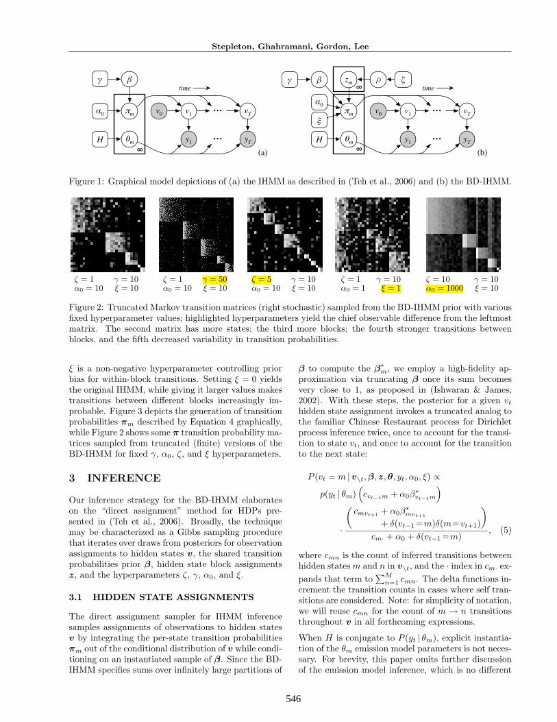
Figure 1: Graphical model depictions of (a) the IHMM as described in (Teh et al., 2006) and (b) the BD-IHMM.

ζ = 1 γ = 10α0 = 10 ξ = 10

ζ = 1 γ = 50α0 = 10 ξ = 10

ζ = 5 γ = 10α0 = 10 ξ = 10

ζ = 1 γ = 10α0 = 1 ξ = 1

ζ = 10 γ = 10α0 = 1000 ξ = 10

Figure 2: Truncated Markov transition matrices (right stochastic) sampled from the BD-IHMM prior with variousfixed hyperparameter values; highlighted hyperparameters yield the chief observable difference from the leftmostmatrix. The second matrix has more states; the third more blocks; the fourth stronger transitions betweenblocks, and the fifth decreased variability in transition probabilities.

ξ is a non-negative hyperparameter controlling priorbias for within-block transitions. Setting ξ = 0 yieldsthe original IHMM, while giving it larger values makestransitions between different blocks increasingly im-probable. Figure 3 depicts the generation of transitionprobabilities πm described by Equation 4 graphically,while Figure 2 shows some π transition probability ma-trices sampled from truncated (finite) versions of theBD-IHMM for fixed γ, α0, ζ, and ξ hyperparameters.

3 INFERENCE

Our inference strategy for the BD-IHMM elaborateson the “direct assignment” method for HDPs pre-sented in (Teh et al., 2006). Broadly, the techniquemay be characterized as a Gibbs sampling procedurethat iterates over draws from posteriors for observationassignments to hidden states v, the shared transitionprobabilities prior β, hidden state block assignmentsz, and the hyperparameters ζ, γ, α0, and ξ.

3.1 HIDDEN STATE ASSIGNMENTS

The direct assignment sampler for IHMM inferencesamples assignments of observations to hidden statesv by integrating the per-state transition probabilitiesπm out of the conditional distribution of v while condi-tioning on an instantiated sample of β. Since the BD-IHMM specifies sums over infinitely large partitions of

β to compute the β∗m, we employ a high-fidelity ap-proximation via truncating β once its sum becomesvery close to 1, as proposed in (Ishwaran & James,2002). With these steps, the posterior for a given vthidden state assignment invokes a truncated analog tothe familiar Chinese Restaurant process for Dirichletprocess inference twice, once to account for the transi-tion to state vt, and once to account for the transitionto the next state:

P (vt = m |v\t,β, z,θ, yt, α0, ξ) ∝

p(yt | θm)(cvt−1m + α0β

∗vt−1m

)

·

(cmvt+1 + α0β

∗mvt+1

+ δ(vt−1 =m)δ(m=vt+1)

)cm· + α0 + δ(vt−1 =m)

, (5)

where cmn is the count of inferred transitions betweenhidden states m and n in v\t, and the · index in cm· ex-pands that term to

∑Mn=1 cmn. The delta functions in-

crement the transition counts in cases where self tran-sitions are considered. Note: for simplicity of notation,we will reuse cmn for the count of m → n transitionsthroughout v in all forthcoming expressions.

When H is conjugate to P (yt | θm), explicit instantia-tion of the θm emission model parameters is not neces-sary. For brevity, this paper omits further discussionof the emission model inference, which is no different

547

The Block Diagonal Infinite Hidden Markov Model

4 8 12

12

4 8 12

1,1,1,1,2,2,2,2,2,3,3,3,4,4,4,4,…z =

β =

ξ12 = 1 + ξ ∕ ∑*

β12 =*

…

…

4 8 12

Possible π12 values:

…

Figure 3: A depiction of the BD-IHMM’s process forgenerating transition probabilities—here, for transi-tions out of hidden state 12. This state has beenassigned block label z12 = 3. (Note: hidden statelabels z are sorted here for clarity, and in the actualmodel there are a countably infinite number of statesassigned to each block.) The shared transition prob-abilities prior parameter β is modified by multiplyingproportions assigned to states in block 3 by the scalarvalue ξ∗12, then renormalizing, yielding a new block-specific parameter β∗12. Next, probabilities for transi-tions out of state 12 are drawn conditioned on β∗12 andthe concentration parameter α0; some possible out-comes are like-colored bars in the bottom graph. Notetransitions to states in block 3 are clearly favored.

from ordinary hierarchical mixture model inference.

3.2 SHARED TRANSITIONS PRIOR

For convenient bookkeeping, the “direct assignment”inference method does not keep some useful informa-tion. In particular, in order to sample the posteriorfor β, we first need to know how many times qmn aparticular transition m → n was selected due to thevt sampler “landing on” the original α0β

∗mn mass al-

located to that transition in (5) rather than transitioncount mass accumulated subsequently. In (Teh et al.,2006), referencing (Antoniak, 1974), this is shown tobe distributed as

P (qmn|cmn, z,β∗, α0) =

s(cmn, qmn)(α0β∗mn)qmn

Γ(α0β∗mn)

Γ(cmn + α0β∗mn), (6)

where s(cmn, qmn) is the unsigned Stirling number ofthe first kind.

We also require a partial instantiation of ρ, the dis-crete distribution yielding block assignments for hid-

den states. If wk =∑Mm=1 δ(zm = k) when summing

only over the M unique states visited during the hid-den state sequence v, then ρk, the probability of draw-ing a particular block label k out of the K unique blocklabels belonging to those states, as well as ρnew, theprobability of drawing any novel block label, is Dirich-let distributed as:

(ρ1, . . . , ρK , ρnew) ∼ Dir(w1, . . . , wk, ζ). (7)

After drawing qmn and ρ, we sample the posterior forboth (a) the β terms corresponding to the M visitedstates and (b) βnew, the sum of β terms for all hithertounvisited states. LetK be the number of unique blocksvisited in v and rk =

∑Mm=1,n=1 qmnδ(zm = k)δ(zn =

k), a sum of within-block transitions. If we now com-pute the ξ∗m as 1 + ξ/(ρzmβnew +

∑Mn=1 βnδ(zn=zm)),

thereby marginalizing over block assignments for theunvisited states, our posterior can be formulated as:

P (β1, . . . , βM , βnew | q, z, ξ, γ) ∝Dir(β1, . . . , βM , βnew; q·1, . . . , q·M , γ)

·K∏k=1

[1 + ξ

/(ρkβnew +

M∑n=1

βnδ(zn=k)

)]rk

. (8)

Sampling this posterior is simplified if theβ1, . . . , βM , βnew are transformed to a new set ofvariables G1, . . . , GK , g1, . . . , gM , βnew, where

Gk =∑Mn=1 βnδ(zn=k), gm = βm

Gzm; (9)

a block-wise sum of and within-block proportions ofβ elements respectively. It can be shown that the gmbelonging to a single block are Dirichlet distributedwith corresponding parameters q·m, and that the Gkand βnew have a density proportional to

βγ−1new

K∏k=1

G−1+

PMn=1 q·nδ(zn=k)

k

(1 +

ξ

ρkβnew +Gk

)rk

.

(10)We sample the above multidimensional density onthe K-simplex with the Multiple-Try Metropolis algo-rithm (Liu et al., 2000), although for large q·n, scalingGk to be proportional to

∑Mn=1 q·n appears to yield a

very close approximation to estimates of its mean.

Once sampled, the Gk and gm variables are trans-formed back into βm proportions, and βnew is subdi-vided into several additional βm proportions for unvis-ited states via a truncated version of the stick-breakingprocess in Equation 1.

3.3 BLOCK ASSIGNMENTS

The posterior over assigning one of the M visited hid-den states m to one of the blocks,

P (zm |ρ,v,β, α0, ξ) ∝ P (zm |ρ)P (v | z,β, α0, ξ),

548

Stepleton, Ghahramani, Gordon, Lee

has two components. The left term is the prior proba-bility of the block assignment, which may be sampledvia a truncated stick-breaking expansion of the ρ pro-portions computed in the prior section. The right termis the likelihood of the sequence of data assignments tohidden states v. For smaller problems, the evaluationof the second term can be shown to be O(M2) as

P (v | z,β, α0, ξ) =M∏m=1

∏Mn=1

Γ(cmn+α0β∗mn)

Γ(α0β∗mn)

Γ(cm·+α0)Γ(α0)

. (11)

Note that the values of the β∗mn change with differentblock assignments zm, as detailed in (4). For largerproblems, a different strategy for sampling the z pos-terior, inspired by the Swendsen-Wang algorithm forMCMC on Potts models (Edwards & Sokal, 1988),changes labels for multiple hidden states simultane-ously, resulting in vastly faster mixing. Space con-straints permit only a sketch of this bookkeeping-intensive technique: for each pair of states, we samplean auxiliary variable indicating whether the bias fortransitions between the same block was responsible forany of the transitions between both states. If this is thecase, both states and any other states so connected tothem must have the same label—in other words, theirnew labels can be resampled simultaneously.

3.4 HYPERPARAMETERS

The hyperparameters α0, ξ, ζ, and γ are positive quan-tities for which we specify Gamma priors. For α0,the sampling method described in (Teh et al., 2006)for the analogous IHMM parameter is directly appli-cable. In the case of ξ, the likelihood term is again(11), which does not permit straightforward sampling.Fortunately, its posterior is amenable to Metropolis-Hastings sampling and appears to exhibit rapid mix-ing. Meanwhile, conditioned on the number of vis-ited blocks K, the ζ posterior may be sampled viathe standard techniques of (Escobar & West, 1995) or(Rasmussen, 2000) (see also (Teh et al., 2006)).

In traditional hierarchical Dirichlet processes, infer-ence for the parameter analogous to the BD-IHMM’sγ relies on marginalizing away β. The required inte-gration is complicated in the BD-IHMM by the sum-mations used in computing β∗m in (4). We use nu-merical methods to capture the γ likelihood instead.When the summed counts q·n described earlier tendto be large, the auxiliary variable-based γ samplingscheme for ordinary HDPs described in (Teh et al.,2006) can be shown to represent a reasonable approxi-mation of the BD-IHMM’s data generating process, atleast with respect to the effects of γ. Because large q·nare not always present, though, especially for shortersequences, we achieve a finer approximation by apply-ing a multiplicative adjustment to the γ value used in

(a) (b) (c)

(d)!!" " !"

!#"

"

#"

!"

500 1000 1500

Figure 4: Results on one 2000-step 2-D syntheticdataset (a) exhibiting four sub-behaviors: dots (col-ored by sub-behavior) are observations, black dot-ted lines connect them in sequence. The matrix oftraining-set transition counts inferred by the IHMM(b) shows conflation of at least three pairs of hiddenstates (yellow shading); the BD-IHMM learns the cor-rect block structure (c). In (d), the sequence of sub-behaviors executed in the training data: inferred (redline) and ground truth (background shading).

this method’s likelihood density. This factor, derivedfrom tens of thousands of runs of the BD-IHMM’sgenerative process with varying hyperparameters, isa function of ζ and M . The use of a multiplicative ad-justment allows the same sampling techniques appliedto ζ and α0 to be used with minimal modification.

4 EXPERIMENTS

4.1 ARTIFICIAL DATA

We compare the results of IHMM and BD-IHMMinference on 100 randomly-generated 2-D datasets.Each is generated by sampling the number of “sub-behaviors” the data should exhibit, then the numbersof states in each sub-behavior. These ranged from 2-4and 3-9 respectively. Means of 2-D spherical Gaussianemission models (σ = 1) were drawn from a larger,sub-behavior specific Gaussian (σ = 6), whose meanin turn was drawn from another Gaussian (σ = 4).Transition probabilities between hidden states favoredwithin-block transitions at a rate of 98%, giving hid-den state sequences within-block “dwelling half lives”of around 34 time steps. Each dataset had 2000 stepsof training data and 2000 steps of test data. Figure4(a) shows one set of sampled observations.

On each dataset we performed IHMM and BD-IHMMinference with vague Gamma priors on all hyperpa-rameters. Emission models used by both the IHMMand BD-IHMM were the same spherical Gaussiansused to sample the data.

549

The Block Diagonal Infinite Hidden Markov Model

0

0.5

1

!!"#""

!!""""

!$#""

!$"""

!%#""

!%"""

!&#""

!&"""

!!"#""

!!""""

!$#""

!$"""

!%#""

!%"""

!&#""

!&"""

(a) (b) (c)

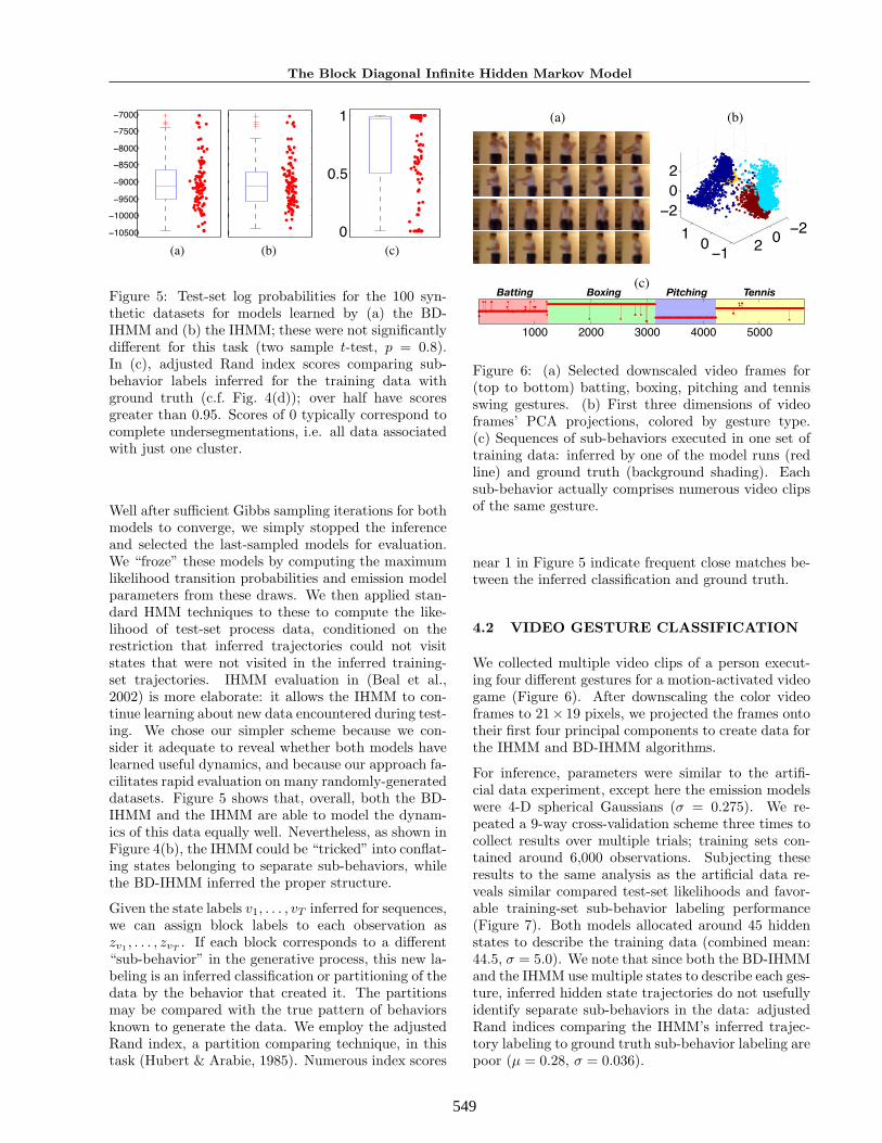
Figure 5: Test-set log probabilities for the 100 syn-thetic datasets for models learned by (a) the BD-IHMM and (b) the IHMM; these were not significantlydifferent for this task (two sample t-test, p = 0.8).In (c), adjusted Rand index scores comparing sub-behavior labels inferred for the training data withground truth (c.f. Fig. 4(d)); over half have scoresgreater than 0.95. Scores of 0 typically correspond tocomplete undersegmentations, i.e. all data associatedwith just one cluster.

Well after sufficient Gibbs sampling iterations for bothmodels to converge, we simply stopped the inferenceand selected the last-sampled models for evaluation.We “froze” these models by computing the maximumlikelihood transition probabilities and emission modelparameters from these draws. We then applied stan-dard HMM techniques to these to compute the like-lihood of test-set process data, conditioned on therestriction that inferred trajectories could not visitstates that were not visited in the inferred training-set trajectories. IHMM evaluation in (Beal et al.,2002) is more elaborate: it allows the IHMM to con-tinue learning about new data encountered during test-ing. We chose our simpler scheme because we con-sider it adequate to reveal whether both models havelearned useful dynamics, and because our approach fa-cilitates rapid evaluation on many randomly-generateddatasets. Figure 5 shows that, overall, both the BD-IHMM and the IHMM are able to model the dynam-ics of this data equally well. Nevertheless, as shown inFigure 4(b), the IHMM could be “tricked” into conflat-ing states belonging to separate sub-behaviors, whilethe BD-IHMM inferred the proper structure.

Given the state labels v1, . . . , vT inferred for sequences,we can assign block labels to each observation aszv1 , . . . , zvT

. If each block corresponds to a different“sub-behavior” in the generative process, this new la-beling is an inferred classification or partitioning of thedata by the behavior that created it. The partitionsmay be compared with the true pattern of behaviorsknown to generate the data. We employ the adjustedRand index, a partition comparing technique, in thistask (Hubert & Arabie, 1985). Numerous index scores

!!"

! !#"

#

!#

"

#

1000 2000 3000 4000 5000

Batting Boxing Pitching Tennis

(a) (b)

(c)

Figure 6: (a) Selected downscaled video frames for(top to bottom) batting, boxing, pitching and tennisswing gestures. (b) First three dimensions of videoframes’ PCA projections, colored by gesture type.(c) Sequences of sub-behaviors executed in one set oftraining data: inferred by one of the model runs (redline) and ground truth (background shading). Eachsub-behavior actually comprises numerous video clipsof the same gesture.

near 1 in Figure 5 indicate frequent close matches be-tween the inferred classification and ground truth.

4.2 VIDEO GESTURE CLASSIFICATION

We collected multiple video clips of a person execut-ing four different gestures for a motion-activated videogame (Figure 6). After downscaling the color videoframes to 21× 19 pixels, we projected the frames ontotheir first four principal components to create data forthe IHMM and BD-IHMM algorithms.

For inference, parameters were similar to the artifi-cial data experiment, except here the emission modelswere 4-D spherical Gaussians (σ = 0.275). We re-peated a 9-way cross-validation scheme three times tocollect results over multiple trials; training sets con-tained around 6,000 observations. Subjecting theseresults to the same analysis as the artificial data re-veals similar compared test-set likelihoods and favor-able training-set sub-behavior labeling performance(Figure 7). Both models allocated around 45 hiddenstates to describe the training data (combined mean:44.5, σ = 5.0). We note that since both the BD-IHMMand the IHMM use multiple states to describe each ges-ture, inferred hidden state trajectories do not usefullyidentify separate sub-behaviors in the data: adjustedRand indices comparing the IHMM’s inferred trajec-tory labeling to ground truth sub-behavior labeling arepoor (µ = 0.28, σ = 0.036).

550

Stepleton, Ghahramani, Gordon, Lee

0

0.5

1

!!"##

!!!##

!!###

!$##

!%##

!!"##

!!!##

!!###

!$##

!%##

(a) (b) (c)

Figure 7: Video gesture dataset log probabilities formodels learned by (a) the BD-IHMM and (b) theIHMM; these were not significantly different (two sam-ple t-test, p = 0.3). In (c), adjusted Rand index scorescomparing sub-behavior labels inferred for the train-ing data with ground truth (c.f. Fig. 6(c)). Most er-rors in labeling were attributable to one of the foursub-behaviors being split into two.

4.3 MUSICAL THEME LABELING

To test the limits of the BD-IHMM’s sub-behavioridentification ability, we used the model to identifymusical themes in a rock song (Collective Soul, 1993).Apart from the challenge of modeling acoustic infor-mation, this dataset is difficult because the themes arelengthy, and no theme is repeated more than four timescontiguously; some sections are only played once. It isuseful to learn whether the BD-IHMM can recognizeseparate sub-behaviors in real-world data with suchlimited repetition.

We prepared a representation of the musical data bycomputing the cepstrums of 113ms windows (yield-ing 2714 observations) of a monophonic signal createdby combining both stereo channels (Childers et al.,1977). We isolated a distinctive quefrency band be-tween 0.9ms and 3.2ms, smoothed the band acrosstime and quefrency with a 2-D Gaussian kernel, thenbinned the quefrencies in each window into 20-bin his-tograms, which, finally, we normalized to sum to 1.The resulting signal appears in Figure 8.

For the hidden-state emission model for the normal-ized histograms, we selected 20-D Dirichlet distribu-tions with a shared, narrow fixed precision and meanslimited to a fixed collection of 500 means generated byrunning K-means on the quefrency histograms. For-saking actual Dirichlet mean estimation for this some-what ad-hoc, discrete prior enables simple and rapidmarginalization of the emission models.

We performed BD-IHMM inference on the dataset29 times, achieving sub-behavior labelings like thoseshown in Figure 8. Fluctuations in the labeling canbe attributed in part to vocal variation in the mu-sic. We compared the labelings with human-generated

1:00 2:00 3:00 4:00 5:00

1:00 2:00 3:00 4:00 5:00

1:00 2:00 3:00 4:00 5:00

Figure 8: Data and results for the musical theme label-ing task. At top, the time series used as input for themodel: normalized quefrency histograms (columns).Below, three sub-behavior (i.e. musical theme) label-ings for the data; inferred labels (red lines) are plottedatop ground truth (background shading).

ground truth and achieved middling adjusted Randindex scores (µ = 0.38, σ = 0.056) due mainly toundersegmentation; whether the representation exhib-ited meaningful variation for different themes may alsobe an issue. Nevertheless, a qualitative evaluation ofthe labelings consistently reveals the discovery of con-siderable theme structure, as exemplified in Figure 8.We conclude that the BD-IHMM is capable of isolat-ing sub-behaviors in datasets with limited repetition,though a task like this one may approach the minimumthreshold for this capability.

4.4 NON-NEGATIVE INTEGERWEIGHTED GRAPH PARTITIONING

Due to the structure of the BD-IHMM, the countsof transitions cmn are a sufficient statistic for infer-ring the hidden state block labels z; the observationsand the actual ordering of the transitions in the pro-cess’s hidden state trajectory are irrelevant. Thesecounts may be represented as non-negative integeredge weights on a directed graph whose vertices cor-respond to the hidden states, and analogously blocklabel inference may be understood as a partitioningof this graph. With this analogy, we show how partsof the BD-IHMM and its inference machinery may beapplied to a different problem domain.

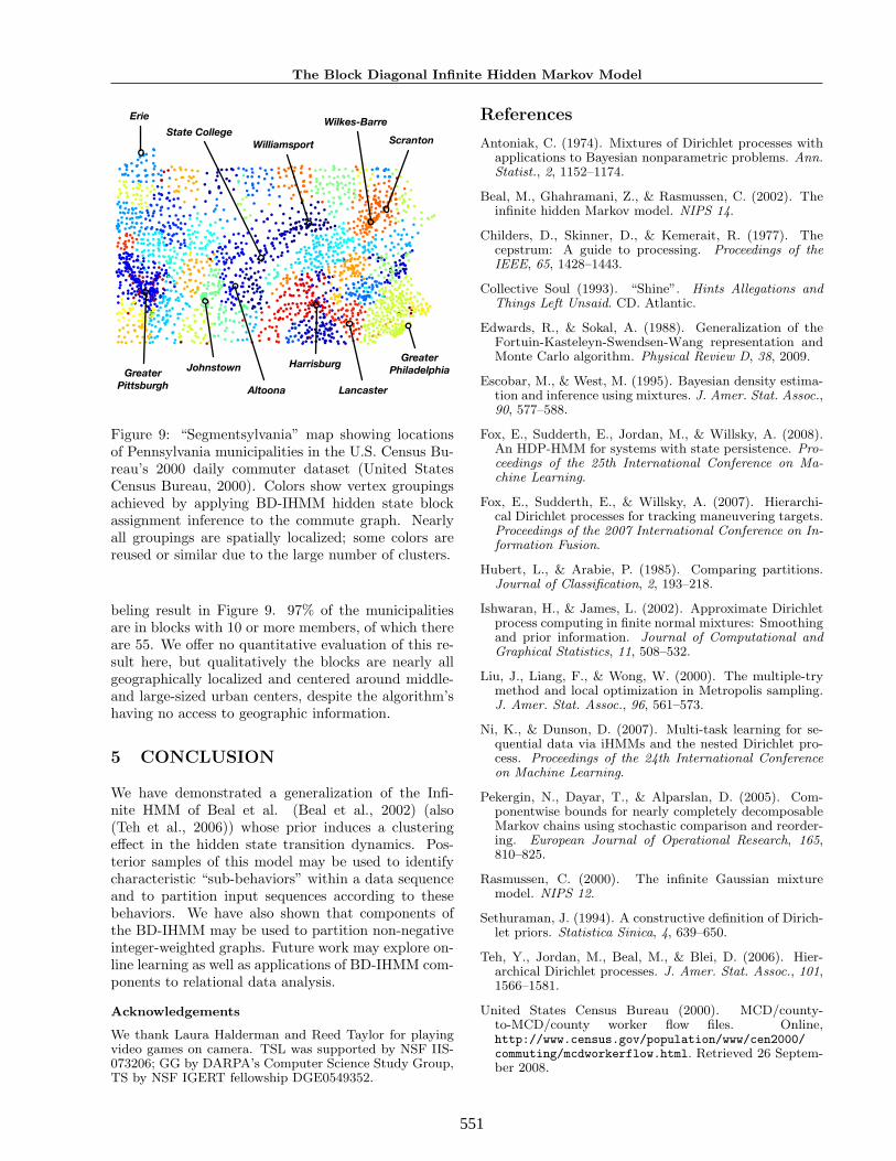
Consider the U.S. Census Bureau’s 2000 dataset onthe daily commuting habits of Pennsylvania residents(United States Census Bureau, 2000). This datasettakes the form of a matrix of counts cmn of the numberof people commuting each day between municipalitiesindexed by m and n. We may assume that this matrixhas a block-diagonal structure, since people are morelikely to commute between areas of shared economicinterest. By finding block labels for the municipalitiesbased on this data, we can identify these regions.

We apply the Swendsen-Wang derived label samplerto the 2580-vertex commute graph, achieving the la-

551

The Block Diagonal Infinite Hidden Markov Model

GreaterPhiladelphiaGreater

Pittsburgh

Harrisburg

Lancaster

Erie

Scranton

Wilkes-Barre

Altoona

Johnstown

WilliamsportState College

Figure 9: “Segmentsylvania” map showing locationsof Pennsylvania municipalities in the U.S. Census Bu-reau’s 2000 daily commuter dataset (United StatesCensus Bureau, 2000). Colors show vertex groupingsachieved by applying BD-IHMM hidden state blockassignment inference to the commute graph. Nearlyall groupings are spatially localized; some colors arereused or similar due to the large number of clusters.

beling result in Figure 9. 97% of the municipalitiesare in blocks with 10 or more members, of which thereare 55. We offer no quantitative evaluation of this re-sult here, but qualitatively the blocks are nearly allgeographically localized and centered around middle-and large-sized urban centers, despite the algorithm’shaving no access to geographic information.

5 CONCLUSION

We have demonstrated a generalization of the Infi-nite HMM of Beal et al. (Beal et al., 2002) (also(Teh et al., 2006)) whose prior induces a clusteringeffect in the hidden state transition dynamics. Pos-terior samples of this model may be used to identifycharacteristic “sub-behaviors” within a data sequenceand to partition input sequences according to thesebehaviors. We have also shown that components ofthe BD-IHMM may be used to partition non-negativeinteger-weighted graphs. Future work may explore on-line learning as well as applications of BD-IHMM com-ponents to relational data analysis.

Acknowledgements

We thank Laura Halderman and Reed Taylor for playingvideo games on camera. TSL was supported by NSF IIS-073206; GG by DARPA’s Computer Science Study Group,TS by NSF IGERT fellowship DGE0549352.

References

Antoniak, C. (1974). Mixtures of Dirichlet processes withapplications to Bayesian nonparametric problems. Ann.Statist., 2, 1152–1174.

Beal, M., Ghahramani, Z., & Rasmussen, C. (2002). Theinfinite hidden Markov model. NIPS 14.

Childers, D., Skinner, D., & Kemerait, R. (1977). Thecepstrum: A guide to processing. Proceedings of theIEEE, 65, 1428–1443.

Collective Soul (1993). “Shine”. Hints Allegations andThings Left Unsaid. CD. Atlantic.

Edwards, R., & Sokal, A. (1988). Generalization of theFortuin-Kasteleyn-Swendsen-Wang representation andMonte Carlo algorithm. Physical Review D, 38, 2009.

Escobar, M., & West, M. (1995). Bayesian density estima-tion and inference using mixtures. J. Amer. Stat. Assoc.,90, 577–588.

Fox, E., Sudderth, E., Jordan, M., & Willsky, A. (2008).An HDP-HMM for systems with state persistence. Pro-ceedings of the 25th International Conference on Ma-chine Learning.

Fox, E., Sudderth, E., & Willsky, A. (2007). Hierarchi-cal Dirichlet processes for tracking maneuvering targets.Proceedings of the 2007 International Conference on In-formation Fusion.

Hubert, L., & Arabie, P. (1985). Comparing partitions.Journal of Classification, 2, 193–218.

Ishwaran, H., & James, L. (2002). Approximate Dirichletprocess computing in finite normal mixtures: Smoothingand prior information. Journal of Computational andGraphical Statistics, 11, 508–532.

Liu, J., Liang, F., & Wong, W. (2000). The multiple-trymethod and local optimization in Metropolis sampling.J. Amer. Stat. Assoc., 96, 561–573.

Ni, K., & Dunson, D. (2007). Multi-task learning for se-quential data via iHMMs and the nested Dirichlet pro-cess. Proceedings of the 24th International Conferenceon Machine Learning.

Pekergin, N., Dayar, T., & Alparslan, D. (2005). Com-ponentwise bounds for nearly completely decomposableMarkov chains using stochastic comparison and reorder-ing. European Journal of Operational Research, 165,810–825.

Rasmussen, C. (2000). The infinite Gaussian mixturemodel. NIPS 12.

Sethuraman, J. (1994). A constructive definition of Dirich-let priors. Statistica Sinica, 4, 639–650.

Teh, Y., Jordan, M., Beal, M., & Blei, D. (2006). Hier-archical Dirichlet processes. J. Amer. Stat. Assoc., 101,1566–1581.

United States Census Bureau (2000). MCD/county-to-MCD/county worker flow files. Online,http://www.census.gov/population/www/cen2000/commuting/mcdworkerflow.html. Retrieved 26 Septem-ber 2008.