Infinite Hidden Markov Switching VARs withApplication to Macroeconomic Forecast

Chenghan Hou∗

Research School of EconomicsAustralian National University

September 9, 2016

Abstract

This paper develops vector autoregressive models with infinite hidden Markovstructures. This is motivated by the recent empirical success of hierarchicalDirichlet process mixture models in financial and macroeconomic applications.We first develop a new Markov chain Monte Carlo (MCMC) method built uponthe precision-based algorithms to improve computational efficiency. We then in-vestigate the forecasting performance of these infinite hidden Markov switchingmodels. Our forecasting results suggest that 1) models with separate infinite hid-den Markov processes for the VAR coefficients and volatilities in general forecastbetter than other specifications of infinite hidden Markov switching models; 2) us-ing a single infinite hidden Markov process to govern all model parameters tendsto forecast poorly; 3) most of the gains in forecasting GDP inflation and GDPgrowth seem to come from allowing for time-variation in volatilities rather thanconditional mean coefficients. In contrast, allowing time-variation in all modelparameters is important in forecasting short-term interest rate.

Keywords: Bayesian nonparametrics, Forecasting, Markov switching, precision,sparse

JEL-Classification: C11, C32, C53, E37

∗I am thankful to my supervisor, Joshua C.C. Chan, for helpful comments. All errors are, ofcourse, my own. Postal address: Research School of Economics, College of Business and Economics,The Australian national University, Canberra ACT 0200, Australia. Email: chenghan.hou@anu.edu.au

Preface

Thesis title: Bayesian mixture models with applications in macroeconomics

Supervisors: Dr. Joshua Chan (Chair), Dr. Tue Gorgens and Dr. John Stachurski

Many macroeconomic time series have been shown to exhibit structural instability.

Bayesian mixture models provide a very flexible framework in modeling this important

feature. The objective of this thesis is to investigate the performance of this class of

models in both in-sample and out-of-sample fit of various macro time series. This thesis

will mainly focus on a number of issues:

1. Scale mixture of Gaussian models and finite Gaussian mixture models

Investigating the forecast performance of the stochastic volatility models under

various disturbance distributional assumptions.

2. Gaussian mixture innovation models with time-varying mixture probability

Reexamining the time-varying relationship between inflation and inflation uncer-

tainty. A Gaussian mixture innovation model with time-varying mixture proba-

bility is proposed to improve the robustness of the estimation results for detecting

in-sample breaks.

3. Infinite hidden Markov mixture models

Evaluating the forecasting performance of various types of autoregressive models

with infinite hidden Markov structures.

The thesis will take the following structure:

Chapter I: Introduction

Chapter II: Stochastic Volatility Models with Alternative Heavy-tailed Distributions

for Forecasting Inflation in G7 countries

Chapter III: Time-Varying Relationship between Inflation and Inflation uncertainty

Chapter IV: Infinite Hidden Markov Switching VARs with Application to Macroeco-

nomic Forecast

Chapter V: Conclusions

This paper is based on the Chapter IV of the thesis.

1

1 Introduction

A voluminous literature has highlighted the wide spread nature of structural instability

in macroeconomic time series (Stock and Watson, 1996; Cogley and Sargent, 2002; Kim

et al., 2004; Koop and Potter, 2007). In order to accommodate such a feature, there has

been an increasing interest in models that allow for time-variation in both conditional

mean coefficients and volatilities. There are two popular families of models often used

in this line of study: time-varying parameters models with stochastic volatility (TVP-

SV) (Cogley and Sargent, 2005; Primiceri, 2005; Liu and Morley, 2014; Koop et al.,

2009; Chan and Eisenstat, 2015) and Markov-switching (MS) models (Sims and Zha,

2006; Geweke and Amisano, 2011; Hubrich and Tetlow, 2015). Many recent studies

have compared alternative specifications of TVP-SV models and found that allowing

for time-variations in conditional mean coefficients and volatilities are important in im-

proving forecast accuracy (D’Agostino et al., 2013; Clark, 2011; Clark and Ravazzolo,

2014). However, there are few papers that focus on the forecasting performance of

MS models, especially in the multivariate setting. This paper contributes to the cur-

rent literature by developing vector autoregressive models with infinite hidden Markov

structures. To improve computational efficiency, we develop a new MCMC sampling

method built upon precision-based algorithms. We then investigate the point and den-

sity forecasting performances of these infinite hidden Markov switching (IMS) models

based on U.S. quarterly GDP inflation, GDP growth and short-term interest rate.

Most recent macroeconomic studies of structural break models and Markov switch-

ing models are restricted to univariate models1. Koop and Potter (2007) extend the

structural break model of Chib (1998) by allowing the number of structural breaks to

be unknown and estimated from data. On the other hand, Giordani and Kohn (2012)

model the random number of structural breaks within the framework of Gaussian state

space model through mixture distributions in the state innovations. Bauwens et al.

(2014) conduct a large forecasting exercise to compare various types of structural break

models and highlight the importance of structural breaks in macroeconomic forecast.

As pointed out by Song (2014), structural break models may incur a loss of estimation

precision, because pre-break data are not directly used in the estimation of parame-

ters of the new born regimes. To this end, he proposes an IMS model with a second

1We refer a structure break model as the model that do not restrict the magnitude of changes inits parameters when a break occurs.

2

hierarchical structure on the model parameters. To allow richer dynamics, Bauwens

et al. (2015) extends the IMS by imposing two independent infinite hidden Markov

processes which are respectively governing the conditional mean coefficients and the

volatilities. However, they have not investigated the forecasting performance of IMS

models with different types of dynamics. In addition, all these studies are limited to

univariate models and have paid little attention to the key practical problem of multi-

variate macroeconomic forecasting under the structural instability. We make two main

contributions to the current literature. First, we extend the IMS models into the frame-

work of vector autoregressive models. Second, we evaluate the forecasting performance

of IMS models with various dynamics in both univariate and multivariate setting.

The IMS model is a nonparametric model built upon the hierarchical Dirichlet pro-

cess of Teh et al. (2006), which extends conventional MS models to allow for a possibly

infinite number of regimes. One of the main advantages of IMS models over MS mod-

els is that its number of regimes for a IMS model needs not be predetermined before

estimation. For a traditional MS model, selecting the number of regimes is essential for

both in-sample inference and out-of-sample forecast performance. This is often done by

comparing or averaging models with different numbers of regimes using a model com-

parison criterion (Hubrich and Tetlow, 2015; Jochmann and Koop, 2015). However,

conducting such a comparison in general is tedious and computationally demanding.

More importantly, it may not be feasible for high dimensional multivariate models.

Motivated by the recent empirical success of the IMS models in many empirical finance

and macroeconomic studies (Jensen and Maheu, 2014; Song, 2014; Jochmann, 2015;

Maheu and Yang, 2015), we adopt the IMS model approach and extend it into the

multivariate setting. To capture the state persistence we consider the sticky version of

IMS model in this paper. We provide a brief discussion about this model in section 2

and refer the readers to Fox et al. (2011) for more details.

First, we contribute to this emerging research by developing vector autoregressive mod-

els with infinite hidden Markov structures. A vast literature has highlighted the em-

pirical importance of allowing for the time-variations in both conditional mean coef-

ficients and volatilities, especially in macroeconomic forecasting (Stock and Watson,

2007; D’Agostino et al., 2013; Clark, 2011; Clark and Ravazzolo, 2014; Chan, 2013,

2015). However, most of these studies are based on the TVP-SV models. For MS

models, as a competitive counterpart of TVP-SV models, there are few studies in the

3

literature that focus on the comparison of MS model with various dynamics. The main

purpose of this paper is to fill this gap. To be specific, this paper compares forecasting

performance of alternative IMS models within the AR and VAR specification and try

to address the following three main issues: 1) whether the IMS model improves the

forecast accuracy upon the time invariant AR or VAR models; 2) whether the findings

in the literature of TVP-SV models are consistent to those of IMS models; 3) which

specification of IMS models performs better comparing with other specifications.

The second contribution of this paper is to propose an algorithm to improve the com-

putational efficiency of estimating IMS models. In order to simulate the regime param-

eters, conventional sampling approach requires regrouping date according to different

regimes. This approach can be slow since the number of regimes for an IMS model is

treated as random and it is possible that a large number of (active) regimes might be

realized in some specific MCMC iterations. Our proposed algorithm allows us to simu-

late the parameters in distinct regime efficiently. The main idea is from the literature of

nonparametric additive regression (Jeliazkov, 2008). To be specific, selection matrices

are constructed on the fly during the estimation process which helps quickly reordering

the data corresponding to distinct regimes. By exploiting the selection matrices, the

precision-based algorithm of Chan and Jeliazkov (2009) can be used to simulate pa-

rameters in distinct regime efficiently.

Third, our recursive out-of-sample forecast exercise shows that time-variation in model

parameters is important for both point and density forecasts. Most of the gains in fore-

casting GDP inflation and GDP growth seem to come from allowing for time-variation

in volatilities rather than conditional mean coefficients. In contrast, allowing for time-

variation in conditional mean coefficients and volatilities are both important in improv-

ing forecast accuracy in short-term interest rate. In addition, models where breaks of

all model parameters occur at the same time in general have poor forecasting perfor-

mance. Furthermore, none of the alternative specifications of IMS models consistently

outperform the model with two independent infinite hidden Markov process: one gov-

erns the changes of the conditional mean coefficients and one governs the changes of

the volatilities.

The rest of the paper is organized as follows. Section 2 briefly discusses the Dirichlet

process and its associated mixture models. Section 3 presents various specifications of

4

IMS models. Section 4 develops an efficient algorithm for estimation. Section 5 first

conducts a posterior analysis, followed by a recursive out-of-sample forecasting exercise

to evaluate the forecasting performance of various specifications of IMS models in both

univariate and multivariate settings. Section 6 concludes.

2 Hierarchical Dirichlet Process Mixture Model

In this section we briefly discuss the Dirichlet process (DP) which is the main building

block of infinite hidden Markov switching models. The Dirichlet process, denoted by

DP(α,G0), is first introduced by Ferguson (1973) and defined as a distribution on

distributions. It is parameterized by a base distribution G0 over a sample space Θ,

and a positive concentration parameter α. For illustrative purpose, we leave the base

distribution G0 unspecified at this stage. Suppose G ∼ DP(α,G0). It can be shown

that G has the following stick-breaking representation (Sethuraman, 1994):

G =∞∑i=1

piδθi , (1)

where δk is the degenerate probability measure at k and θi ∼ G0 for i = 1, 2, . . .. The

probability weights p = (p1, p2, . . .) are obtained from a stick-breaking process

Vi ∼ B(1, α), pi = Vi

i−1∏j=1

(1− Vj), (2)

where B(·, ·) represents the Beta distribution. We denote the process in (2) as p ∼SBP(α). It is worth noting that a draw p ∼ SBP(α) satisfies

∑∞i=1 pi = 1 and can be

interpreted as a distribution over natural number. Intuitively, the process in (2) can be

thought of as breaking a stick of unit length infinitely many times. At the ith time of

breaking the stick, a draw Vi ∼ B(1, α) will determine the proportion of the remaining

stick to be broken.

The discrete nature of the DP makes it well suited for a prior in nonparametric mixture

modeling. Let (y1, . . . , yT ) be the variables of interest. The generic form of a Dirichlet

5

process mixture model can be written as

yt|st, θi∞i=1 ∼ F (θst), (3)

θi ∼ G0, (4)

st ∼ p, (5)

p ∼ SBP(α), (6)

where st is the state variable taking values over natural number and F is a distribution

parameterized by θi. We leave F to be unspecified for now and will discuss more about it

in section 3. The Dirichlet process mixture model described above can be thought of as

an extension of the finite mixture model to an infinite number of mixture components.

However, the lack of state dependency makes the Dirichlet process mixture model less

suitable for time series analysis. To this end, Teh et al. (2006) introduce a hierarchical

DP prior to a set of Dirichlet process mixture models. This allows those Dirichlet

process mixture models to be related and share information to each other through the

hierarchical structure. The infinite hidden Markov switching model is one important

variant of the hierarchical DP mixture model. Its generic form can be represented as

yt|st, θi∞i=1 ∼ F (θst), (7)

θi ∼ G0, (8)

st|st−1, pi∞i=1 ∼ pst−1 , (9)

pi|α,π ∼ DP(α,π), (10)

π|γ ∼ SBP(γ), (11)

From equation (9), we can see that the state variable st follows a first order Markov

process. As each pi is an infinite dimensional vector, st can be thought of as following

a Markov process which is governed by an infinite dimensional transitional matrix. In

addition, all pi are drawn from the common distribution DP(α,π), this allows them to

learn and share information with each other.

As many macroeconomic time series are evolving with high persistence, the sticky

version of the Dirichlet process prior is more suitable in modeling such a feature (Fox

et al., 2011). To be specific, the sticky version of an infinite hidden Markov switching

6

model is defined as the same as (7) - (11) but with equation (10) replaced by

pi|α,π ∼ DP(c, (1− ρ)π + ρδi), (12)

where 0 < ρ < 1 is referred as the sticky parameter which reinforces the state self-

transition probability. As different values of parameters (ρ, c, γ) reflect different belief

of the hidden Markov process, instead of setting them to specific values, we treat them

as parameters to be estimated. A brief overview of the MCMC estimation is presented

in section 4. More details are provided in the Appendix. We refer readers to Teh et al.

(2006); Jochmann (2015) for more discussions about the DP and its associated mixture

models.

3 Infinite Hidden Markov Switching VAR

In this section, we discuss three specifications of infinite hidden Markov switching vector

autoregressive model. To set the stage, let (y1, . . . ,yT ) be the T observed variables of

interest and each yt is a n× 1 vector. We consider a VAR(q) model:

yt = cst + A1,styt−1 + · · ·+ Aq,styt−q + εt, εt ∼ N (0,Σst), (13)

where N (·, ·) denotes the Gaussian distribution, cst is an n × 1 vector of intercepts,

A1,st , . . . ,Aq,st are n × n coefficient matrices and Σst is the n × n covariance matrix.

We rewrite equation (13) as a linear regression model

yt = Xtβst + εt, εt ∼ N (0,Σst), (14)

where βst = vec ((cst ,A1,st , . . . ,Aq,st)′) is kβ × 1 with kβ = n(nq + 1) and Xt =

In ⊗ (1,y′t−1, . . . ,y′t−q). The time-variation of the VAR coefficients βst and covariance

Σst are determined by the regime indicator variable st ∈ 1, 2, . . . which is following a

infinite hidden Markov process:

st|st−1, pi∞i=1 ∼ pst−1 , (15)

pi|c, ρ,π ∼ DP(c, (1− ρ)π + ρδi), (16)

π|γ ∼ SBP(γ), (17)

(βi,Σi) ∼ G(β,Σ), (18)

7

where G(βi,Σi) denotes the base distribution which generates the regime parameters.

We refer the model (14) - (18) as IMS-VAR(q). The IMS-VAR(q) assumes that both

βst and Σst are governed by a single infinite hidden Markov process. This implies that

the breaks in the VAR coefficients and the volatilities have to occur at the same time.

To allow for richer dynamics, we also consider a version that incorporates two indepen-

dent infinite hidden Markov processes: one governs the changes of the VAR coefficients

and the other governs the changes of the volatilities. To be specific, we consider the

model:

yt = Xtβst + εt, εt ∼ N (0,Σzt), (19)

st|st−1, psi∞i=1 ∼ psst−1, (20)

psi |cs, ρs,πs ∼ DP(cs, (1− ρs)πs + ρsδi), (21)

πs|γs ∼ SBP(γs), (22)

zt|zt−1, pzi ∞i=1 ∼ pzzt−1, (23)

pzi |cz, ρz,πz ∼ DP(cz, (1− ρz)πz + ρzδi), (24)

πz|γz ∼ SBP(γz), (25)

βi ∼ Gβ, Σi ∼ GΣ. (26)

We refer to this VAR model which consists of double infinite hidden Markov processes

as DIMS-VAR(q). The main difference of DIMS-VAR(q) from IMS-VAR(q) is that the

variations of βst and Σzt depend respectively on st and zt, which are independent of

each other. This can also be seen by comparing the base distributions in equation (18)

and (26). In IMS-VAR(q), all model parameters are generated from a single base dis-

tribution G(β,Σ). In contrast two base distributions, Gβ and GΣ, are incorporated in

DIMS-VAR(q) which generates βst and Σzt independently.

Many studies have found that the conditional mean coefficients of a VAR model are less

likely to be varying over time (Primiceri, 2005; Koop et al., 2009; Chan and Eisenstat,

2015). Based on this reason, we consider a VAR model with constant conditional mean

8

coefficients:

yt = Xtβ + εt, εt ∼ N (0,Σzt), (27)

zt|zt−1, pzi ∞i=1 ∼ pzzt−1, (28)

pzi |cz, ρz,πz ∼ DP(cz, (1− ρz)πz + ρzδi), (29)

πz|γz ∼ SBP(γz), (30)

Σi ∼ GΣ, (31)

and we refer to this model as C-VAR(q)-IMS.

To complete model specification, we specify our base distribution of DIMS-VAR(q)

and IMS-VAR(q) as,

βi ∼ N (β0,V0), Σ−1i ∼ W(Σ−1

0 , ν0). (32)

For C-VAR(q)-IMS, we assume the priors for the VAR coefficients and base distribution

of the covariance matrix as

β ∼ N (βc,Vc), Σ−1i ∼ W(Σ−1

0 , ν0) (33)

As proposed by Song (2014), imposing a second hierarchical structure on the base

distribution allows for regime parameters in the new born regime to learn from the

existing regimes, which helps improving the forecast accuracy. We follow his approach

and set the second hierarchical priors as

β0 ∼ N (β00,B00), V−10 ∼ W(A00, a00), Σ0 ∼ W(Q00, b00), ν0 ∼ E(λ00)1(ν0 > n),

(34)

where W(S, ν) denotes the Wishart distribution with scale matrix S and degrees of

freedom ν. E(λ) denotes the exponential distribution with mean λ. The indicator

function 1(ν0 > n) implies that the support of the prior for ν0 is restricted to be

greater than n. Lastly, we assume the hyperparameters (cs, cz, γs, γz, ρs, ρz) to follow

9

independent priors given as

cs ∼ G(ws, θs), γs ∼ G(hs, ηs), ρs ∼ B(fs, gs), (35)

cz ∼ G(wz, θz), γz ∼ G(hz, ηz), ρz ∼ B(fz, gz), (36)

where G(κ1, κ2) denotes the Gamma distribution with mean κ1/κ2 and variance κ1/κ22.

4 Bayesian Estimation

This section provides an overview of the Markov chain Monte Carlo (MCMC) posterior

sampler for model estimation. To be concise, we focus on the estimation procedure of

the DIMS-VAR(q) model. Only minor modifications are needed for the estimation of

the other models. For notational convenience, let s = (s1, . . . , sT ), z = (z1, . . . , zT ),

Hs = (cs, γs, ρs), Hz = (cz, γz, ρz), Φ = (β0,V0,Σ0, ν0) and Ps = (ps1′,ps2

′, . . .)′,

Pz = (pz1′,pz2

′, . . .)′. We also use Θ to denote the collection of all regime parameters,

i.e. Θ =(βi∞i=1, Σj∞j=1

). Since IMS models allow for a possibly infinite number of

states, the algorithm of Chib (1996) that handles a finite number of states cannot be

applied. One approach is to work only with a large finite number of states to approx-

imate the IMS model (Fox et al., 2011; Jochmann, 2015). In contrast, we follow the

approach of beam sampler proposed by Van Gael et al. (2008) for obtaining samples

from the exact posterior distribution.

To apply the beam sampler, auxiliary variables us = (us1, . . . , usT ) and uz = (uz1, . . . , u

zT )

are introduced such that they are sampled alongside with the other model parameters,

but they do not change the marginal distributions of the other model parameters. To

be specific, for each t, ust is introduced with conditional density

p(ust |st−1, st) =p(ust , st|st−1)

p(st|st−1)=1(0 < ust < psst−1st

)

psst−1st

. (37)

We suppress the rest of the conditioning variables for notational simplicity. This im-

plies that the joint density of (ust , st) given st−1 is p(ust , st|st−1) = 1(0 < ust < psst−1st).

Apparently, marginalizing out ust returns the original model. Hence sampling us along-

side with the other model parameters does not change the marginal distributions of the

10

other model parameters. In addition, the conditional density of st given (ust , st−1) is

p(st|ust , st−1) =1(0 < ust < psst−1st

)∑i 1(0 < ust < psst−1i

). (38)

As∑

i psst−1i

= 1, it is not hard to see that the set i : 0 < ust < psst−1i is finite. This

implies that, given us, there is only a finite number of state trajectory needed to be

considered. Thus the algorithm of Chib (1996) can be applied to obtain samples of the

state variables s. The samples for the state variables z can also be obtained using a

similar approach. More details about the beam sampler can be found in Van Gael et al.

(2008) and the Appendix.

The posterior draws for the DIMS-VAR(q) model can be obtained by sequentially sam-

pling from:

1. p(Θ|s, z,πs,πz,Ps,Pz,us,uz,Hs,Hz,Φ,y1:T ) = p(Θ|Φ, s, z);

2. p(Φ|s, z,πs,πz,Ps,Pz,Hs,Hz,us,uz,Θ,y1:T ) = p(Φ|Θ, s, z);

3. p(us,uz|s, z,πs,πz,Ps,Pz,Hs,Hz, ,Θ,Φ,y1:T ) = p(us,uz|s, z,Ps,Pz)

4. p(s, z|πs,πz,Ps,Pz,Hs,Hz,us,uz,Θ,Φ,y1:T ) = p(s, z|Ps,Pz,πs,πz,us,uz,Θ,y1:T );

5. p(πs,πz|s, z,Ps,Pz,Hs,Hz,us,uz,Θ,Φ,y1:T ) = p(πs,πz|s, z,Hs,Hz);

6. p(Ps,Pz|s, z,πs,πz,us,uz,Hs,Hz,Θ,Φ,y1:T ) = p(Ps,Pz|s, z,πs,πz,Hs,Hz);

7. p(Hs,Hz|s, z,πs,πz,Ps,Pz,us,uz,Θ,Φ,y1:T ) = p(Hs,Hz|s, z,Ps,Pz).

A regime is said to be active if at least one observation belongs to it. It is worth noting

that conditional on the auxiliary variables us and uz, there is only a finite number of

active regimes. We denote Ls and Lz as the numbers of active regimes implied by s and z

respectively. To improve computational efficiency, we propose an efficient way to obtain

samples from p(Θ|Φ, s, z) in step 1. The idea is from the literature of nonparametric

additive regression (Jeliazkov, 2008). In our proposed approach, selection matrices

are constructed on the fly in each MCMC iteration to avoid explicitly regouping the

data into distinct regimes. To be specific, we first stack all T observations and rewrite

equation (14) as

Y = XB + ε, ε ∼ N (0,Ω), (39)

11

where

X =

X1 0 · · · 0

0 X2 · · · 0...

.... . .

...

0 0 · · · XT

, Ω =

Σz1 0 · · · 0

0 Σz2 · · · 0...

.... . .

...

0 0 · · · ΣzT

,

and Y = (y′1, . . . ,y′T )′ and B = (β′s1 , . . . ,β

′sT

)′.

It is important to note that only the VAR coefficients for distinct active regimes,

B = (β′1, . . . ,β′Ls)′, are needed to be sampled in each MCMC iteration. To improve

efficiency, we define a T ×Ls selection matrix Ds which has entry Ds(i, j) = 1 if si = j

and 0 otherwise. It is easy to check that B =(Ds ⊗ Ikβ

)B. Hence equation (39) can

be written as

Y = XsB + ε, ε ∼ N (0,Ω), (40)

where Xs = X(Ds ⊗ Ikβ

). Equation (40) is in the form of linear regression model, a

standard result can be applied to obtain draws of B from

B ∼ N(B,VB

), (41)

where V−1B =

(Xs′Ω−1Xs + V−1

Ls

), B = VB

(Xs′Ω−1Y + V−1

LsβLs

), VLs = ILs ⊗ V0,

βLs

= 1Ls ⊗ β0. 1Ls is a Ls × 1 column vector with all one at each entry.

To obtain draws of Σi for i = 1, . . . , Lz, we apply a similar trick to sort out the

data by using a selection matrix. To be specific, given draws of B, s and z we first

construct

Yd =

(y1 −X1βs1

) (y1 −X1βs1

)′(y2 −X2βs2

) (y2 −X2βs2

)′...(

yT −XTβsT) (

yT −XTβsT)′

, (42)

and a Lz × T selection matrix Dz that has Dz(i, j) = 1 if zj = i and 0 otherwise. It is

12

straightforward to check that

(Dz ⊗ In) Yd =

∑

t:zt=1

(yt −Xtβst

) (yt −Xtβst

)′∑t:zt=2

(yt −Xtβst

) (yt −Xtβst

)′...∑

t:zt=Lz

(yt −Xtβst

) (yt −Xtβst

)′

, (43)

then for i = 1, . . . , Lz sample Σi ∼ IW(∑

t:zt=i

(yt −Xtβst

) (yt −Xtβst

)′+ Σ0, ν0 + Ti

),

where Ti =∑

j Dz(i, j).

We make two remarks on the computation. First, it is important to observe that the

kβLs × kβLs matrix V−1B is block-banded i.e., all non-zero elements are concentrated

around the main diagonal. This structure can be exploited to efficiently compute B

without calculating the inverse of V−1B . In addition, the precision-based sampler of

Chan and Jeliazkov (2009) can be applied to quickly obtain draws from N (B,VB).

Second, in principle the number of active regimes in the framework of IMS model can

be as large as the sample size T . In the traditional approach, parameters are sampled

sequentially after regrouping the data into distinct regimes in each MCMC iteration.

The computational efficiency is low especially when a large number of active regimes is

realized at some specific MCMC iterations. Our proposed approach vectorizes all the

operations through constructing selection matrices on the fly during estimation, which

is very fast in programming environments such as MATLAB, GAUSS and R.

Table 1 reports the time taken to obtain 10000 posterior draws for various types of

IMS models with 2 lags. The computational times for two univariate IMS models,

DIMS-AR and IMS-AR, are also reported2. More specifically, the DIMS-AR (IMS-

AR) is the DIMS-VAR (IMS-VAR) with n = 1. We use U.S. quarterly GDP inflation

rate, GDP growth and short-term interest rate from 1954Q3 - 2015Q1 with a total of

T = 241 observations. We will discuss more about the data in the next section. All the

algorithms are implemented using MATLAB on a desktop with an Intel Core i7-2600

@3.40GHz processor.

2The computational times for the univariate models, DIMS-AR and DIMS-AR, are the averageestimation times for GDP inflation rate, GDP growth and short-term interest rate.

13

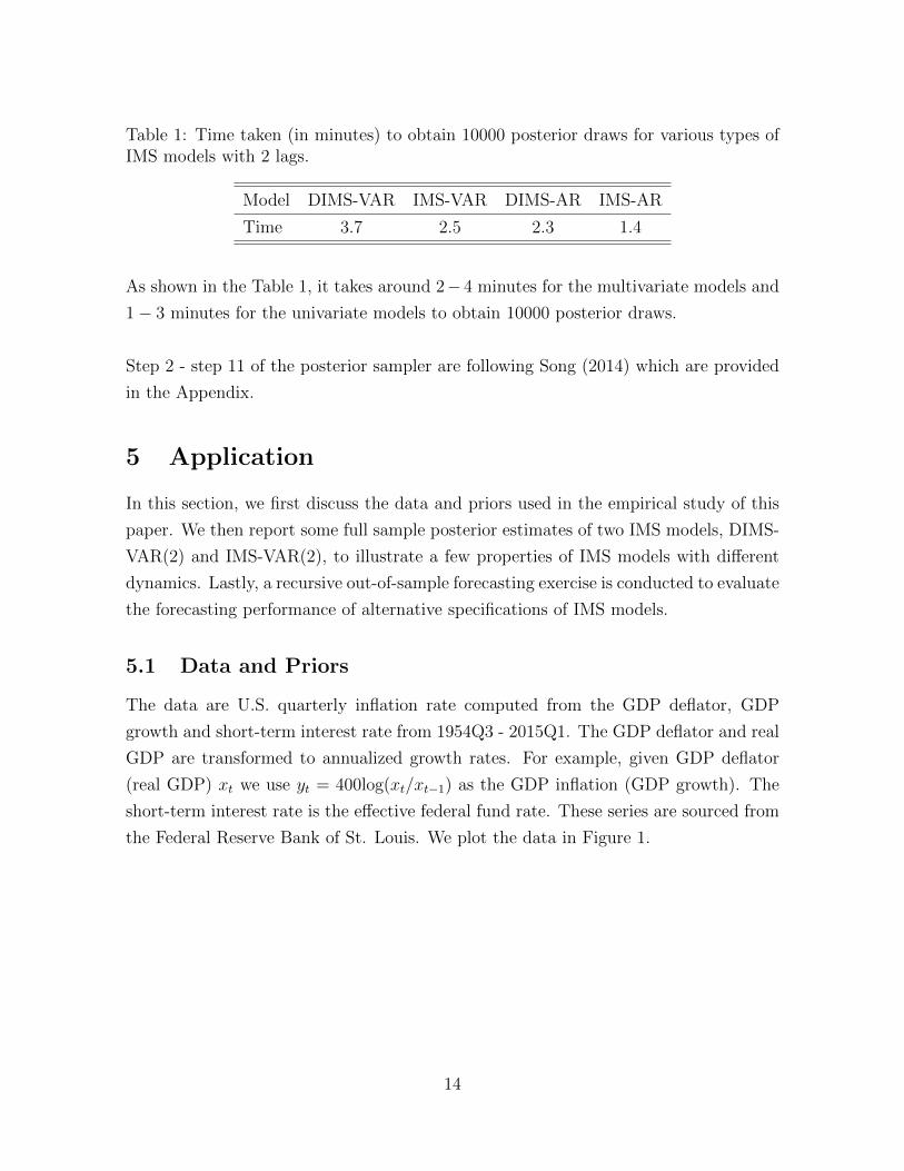
Table 1: Time taken (in minutes) to obtain 10000 posterior draws for various types ofIMS models with 2 lags.

Model DIMS-VAR IMS-VAR DIMS-AR IMS-AR

Time 3.7 2.5 2.3 1.4

As shown in the Table 1, it takes around 2− 4 minutes for the multivariate models and

1− 3 minutes for the univariate models to obtain 10000 posterior draws.

Step 2 - step 11 of the posterior sampler are following Song (2014) which are provided

in the Appendix.

5 Application

In this section, we first discuss the data and priors used in the empirical study of this

paper. We then report some full sample posterior estimates of two IMS models, DIMS-

VAR(2) and IMS-VAR(2), to illustrate a few properties of IMS models with different

dynamics. Lastly, a recursive out-of-sample forecasting exercise is conducted to evaluate

the forecasting performance of alternative specifications of IMS models.

5.1 Data and Priors

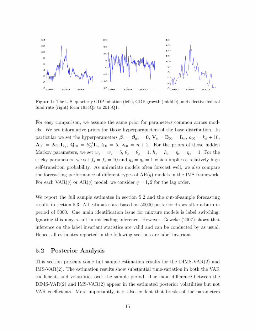
The data are U.S. quarterly inflation rate computed from the GDP deflator, GDP

growth and short-term interest rate from 1954Q3 - 2015Q1. The GDP deflator and real

GDP are transformed to annualized growth rates. For example, given GDP deflator

(real GDP) xt we use yt = 400log(xt/xt−1) as the GDP inflation (GDP growth). The

short-term interest rate is the effective federal fund rate. These series are sourced from

the Federal Reserve Bank of St. Louis. We plot the data in Figure 1.

14

1960 1980 2000−2

0

2

4

6

8

10

12

14

1960 1980 2000−15

−10

−5

0

5

10

15

20

1960 1980 20000

2

4

6

8

10

12

14

16

18

Figure 1: The U.S. quarterly GDP inflation (left), GDP growth (middle), and effective federalfund rate (right) form 1954Q3 to 2015Q1.

For easy comparison, we assume the same prior for parameters common across mod-

els. We set informative priors for those hyperparameters of the base distribution. In

particular we set the hyperparameters βc = β00 = 0, Vc = B00 = Ikβ , a00 = kβ + 10,

A00 = 2a00Ikβ , Q00 = b−100 In, b00 = 5, λ00 = n + 2. For the priors of those hidden

Markov parameters, we set ws = wz = 5, θs = θz = 1, hs = hz = ηs = ηz = 1. For the

sticky parameters, we set fs = fz = 10 and gs = gz = 1 which implies a relatively high

self-transition probability. As univariate models often forecast well, we also compare

the forecasting performance of different types of AR(q) models in the IMS framework.

For each VAR(q) or AR(q) model, we consider q = 1, 2 for the lag order.

We report the full sample estimates in section 5.2 and the out-of-sample forecasting

results in section 5.3. All estimates are based on 50000 posterior draws after a burn-in

period of 5000. One main identification issue for mixture models is label switching.

Ignoring this may result in misleading inference. However, Geweke (2007) shows that

inference on the label invariant statistics are valid and can be conducted by as usual.

Hence, all estimates reported in the following sections are label invariant.

5.2 Posterior Analysis

This section presents some full sample estimation results for the DIMS-VAR(2) and

IMS-VAR(2). The estimation results show substantial time-variation in both the VAR

coefficients and volatilities over the sample period. The main difference between the

DIMS-VAR(2) and IMS-VAR(2) appear in the estimated posterior volatilities but not

VAR coefficients. More importantly, it is also evident that breaks of the parameters

15

are not likely to occur at the same time.

Figure 2 - Figure 5 plot the estimated posterior means (solid lines) for the VAR coef-

ficients and covariance matrices with the corresponding 68% credible intervals (dashed

lines) for the DIMS-VAR(2) and IMS-VAR(2). In Figure 2 and Figure 3, each row

plots the coefficients for one equation and each column reports the coefficients for one

variables. For example, the third panel in the first row plots the coefficients of the first

lagged GDP growth in the equation of inflation.

Overall, the estimates of the VAR coefficients from both models are mostly the same

over the sample period. There are cases that the estimated 68% credible intervals of

some coefficients for DIMS-VAR(2) and IMS-VAR(2) almost exclude each other, but

the difference of their posterior means are small. For example, in the equation of in-

terest rate, the 68% credible intervals of the coefficients of the first lag interest rate for

DIMS-VAR(2) and IMS-VAR(2) barely exclude each other in most periods, however

the difference of their posterior means is only around 0.2.

Figure 4 and Figure 5 plots the estimates of the covariance matrices for the DIMS-

VAR(2) and IMS-VAR(2) models. We use 1, 2, 3 to label the equation of inflation,

GDP growth and interest rate accordingly. Thus, σij denotes the covariance of innova-

tions in equation i and equation j. For example, σ11 is the variance of the innovation

in the equation of inflation. The estimated covariance matrices for both models in-

dicate that the volatilities of the innovations are typically high in the 1970s, followed

by a decline in the early 1980s. This finding is generally consistent with the studies

of the Great Moderation (Chan and Eisenstat, 2015; Primiceri, 2005; Sims and Zha,

2006). However the estimates for the DIMS-VAR(2) detect a drastic rise in volatilities

during the Global Financial Crisis in the late 2000s. In contrast, there are no notable

changes have been found in the volatilities during the whole 2000s from the estimates

of the IMS-VAR(2). Furthermore, the estimated covariance among variables for the

IMS-VAR(2) are much larger comparing with those for the DIMS-VAR(2) in this high

volatile period.

16

1960 1980 20000

0.2

0.4

Constant I

nfla

tion

1960 1980 20000.3

0.4

0.5

0.6

inf(−1)

1960 1980 2000−0.1

0

0.1 gdp(−1)

1960 1980 2000

0.1

0.2

0.3

0.4 int(−1)

1960 1980 2000

0.2

0.3

0.4 inf(−2)

1960 1980 2000−0.05

0

0.05

0.1 gdp(−2)

1960 1980 2000

−0.2

−0.1

0

int(−2)

1960 1980 20001.5

2

2.5

Constant

GD

P g

row

th

1960 1980 2000

0

0.2

0.4

inf(−1)

1960 1980 2000

0.2

0.3

0.4 gdp(−1)

1960 1980 2000

−0.4

−0.2

0

0.2

int(−1)

1960 1980 2000

−0.4

−0.2

0

inf(−2)

1960 1980 20000

0.1

0.2

0.3 gdp(−2)

1960 1980 2000

−0.2

0

0.2

0.4

int(−2)

1960 1980 2000

−0.4

−0.2

0 Constant

In

tere

st r

ate

1960 1980 2000

0

0.1

0.2 inf(−1)

1960 1980 2000

0

0.05

0.1

gdp(−1)

1960 1980 2000

1

1.2

1.4

int(−1)

1960 1980 2000

0

0.1

0.2

inf(−2)

1960 1980 2000−0.1

0

0.1

gdp(−2)

1960 1980 2000

−0.4

−0.2

0 int(−2)

Figure 2: The estimated VAR coefficients for the DIMS-VAR(2): Each row reports estimatesfor the corresponding equation. Each column reports estimates of the lag variables.

1960 1980 20000

0.2

0.4

Constant

Infla

tion

1960 1980 20000.3

0.4

0.5

0.6

inf(−1)

1960 1980 2000−0.1

0

0.1 gdp(−1)

1960 1980 2000

0.1

0.2

0.3

0.4 int(−1)

1960 1980 2000

0.2

0.3

0.4 inf(−2)

1960 1980 2000−0.05

0

0.05

0.1 gdp(−2)

1960 1980 2000

−0.2

−0.1

0

int(−2)

1960 1980 20001.5

2

2.5

Constant

GD

P g

row

th

1960 1980 2000

0

0.2

0.4

inf(−1)

1960 1980 2000

0.2

0.3

0.4 gdp(−1)

1960 1980 2000

−0.4

−0.2

0

0.2

int(−1)

1960 1980 2000

−0.4

−0.2

0

inf(−2)

1960 1980 20000

0.1

0.2

0.3 gdp(−2)

1960 1980 2000

−0.2

0

0.2

0.4

int(−2)

1960 1980 2000

−0.4

−0.2

0 Constant

Inte

rest

rat

e

1960 1980 2000

0

0.1

0.2 inf(−1)

1960 1980 2000

0

0.05

0.1

gdp(−1)

1960 1980 2000

1

1.2

1.4

int(−1)

1960 1980 2000

0

0.1

0.2

inf(−2)

1960 1980 2000−0.1

0

0.1

gdp(−2)

1960 1980 2000

−0.4

−0.2

0 int(−2)

Figure 3: The estimated VAR coefficients for the IMS-VAR(2): Each row reports estimatesfor the corresponding equation. Each column reports estimates of the lag variables.

17

1960 1970 1980 1990 2000 20100

2.5

5

σ11

1960 1970 1980 1990 2000 2010−4

0

4

8

σ21

1960 1970 1980 1990 2000 20100

2

4

σ31

1960 1970 1980 1990 2000 2010−4

0

4

8

σ12

1960 1970 1980 1990 2000 20100

20

40

σ22

1960 1970 1980 1990 2000 2010

0

5

10

σ32

1960 1970 1980 1990 2000 20100

2

4

σ13

1960 1970 1980 1990 2000 2010

0

5

10

σ23

1960 1970 1980 1990 2000 20100

5

10

σ33

Figure 4: The estimated covariance matrix for the DIMS-VAR(2).

1960 1970 1980 1990 2000 20100

2.5

5

σ11

1960 1970 1980 1990 2000 2010−4

0

4

8

σ21

1960 1970 1980 1990 2000 20100

2

4

σ31

1960 1970 1980 1990 2000 2010−4

0

4

8

σ12

1960 1970 1980 1990 2000 20100

20

40

σ22

1960 1970 1980 1990 2000 2010

0

5

10

σ32

1960 1970 1980 1990 2000 20100

2

4

σ13

1960 1970 1980 1990 2000 2010

0

5

10

σ23

1960 1970 1980 1990 2000 20100

5

10

σ33

Figure 5: The estimated covariance matrix for the IMS-VAR(2).

Figure 6 and Figure 7 display the estimated posterior distributions of the numbers of

the active regimes for the DIMS-VAR(2) and IMS-VAR(2). These figures show that the

regime uncertainty has been taken into account by both models. Moreover it is obvious

that the shape of these posterior distributions are very different from each other. As

18

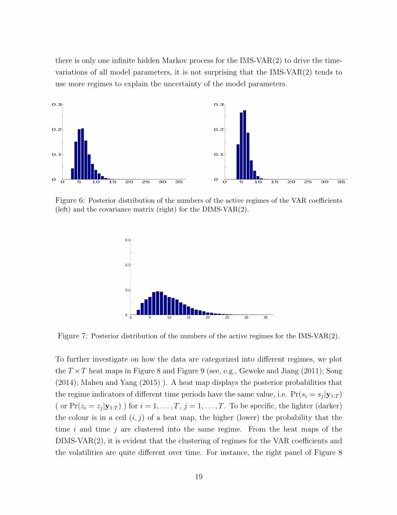
there is only one infinite hidden Markov process for the IMS-VAR(2) to drive the time-

variations of all model parameters, it is not surprising that the IMS-VAR(2) tends to

use more regimes to explain the uncertainty of the model parameters.

0 5 10 15 20 25 30 350

0.1

0.2

0.3

0 5 10 15 20 25 30 350

0.1

0.2

0.3

Figure 6: Posterior distribution of the numbers of the active regimes of the VAR coefficients(left) and the covariance matrix (right) for the DIMS-VAR(2).

0 5 10 15 20 25 30 350

0.1

0.2

0.3

Figure 7: Posterior distribution of the numbers of the active regimes for the IMS-VAR(2).

To further investigate on how the data are categorized into different regimes, we plot

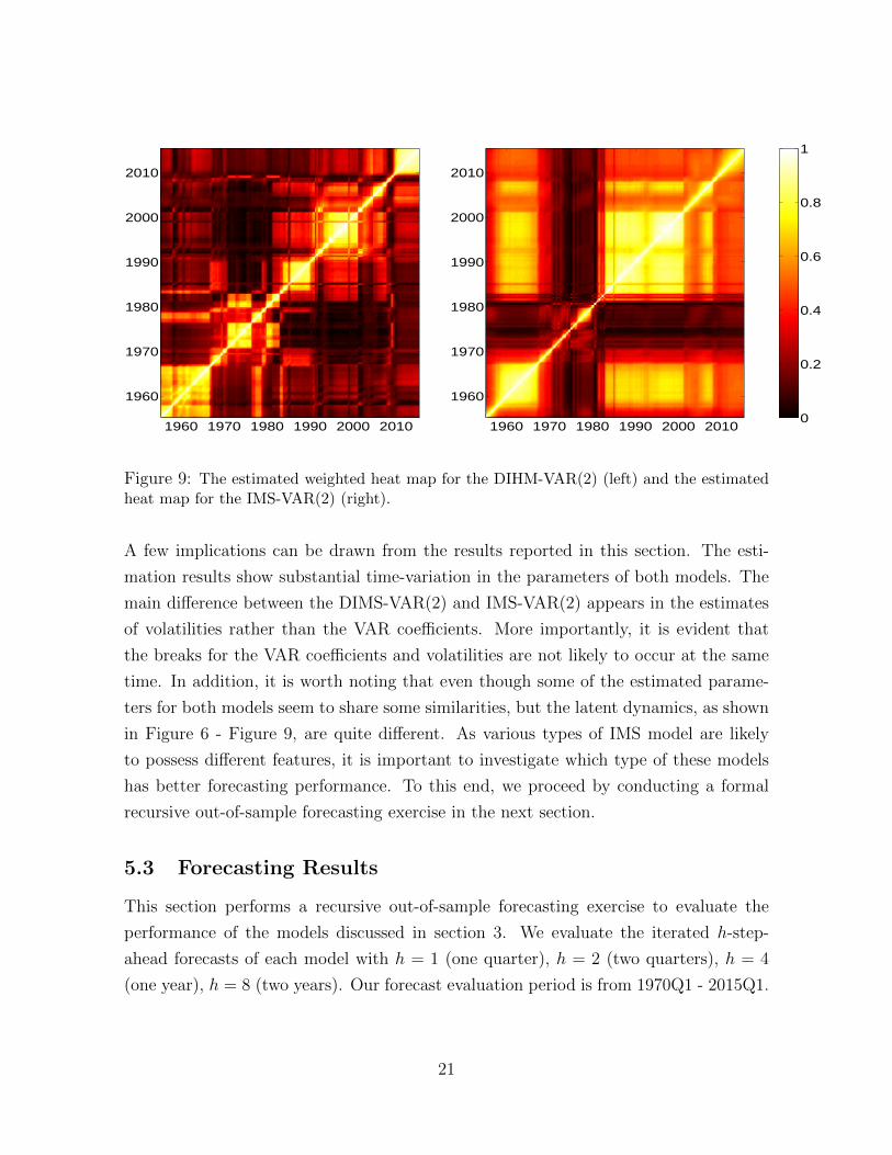
the T ×T heat maps in Figure 8 and Figure 9 (see, e.g., Geweke and Jiang (2011); Song

(2014); Maheu and Yang (2015) ). A heat map displays the posterior probabilities that

the regime indicators of different time periods have the same value, i.e. Pr(si = sj|y1:T )

( or Pr(zi = zj|y1:T ) ) for i = 1, . . . , T , j = 1, . . . , T . To be specific, the lighter (darker)

the colour is in a ceil (i, j) of a heat map, the higher (lower) the probability that the

time i and time j are clustered into the same regime. From the heat maps of the

DIMS-VAR(2), it is evident that the clustering of regimes for the VAR coefficients and

the volatilities are quite different over time. For instance, the right panel of Figure 8

19

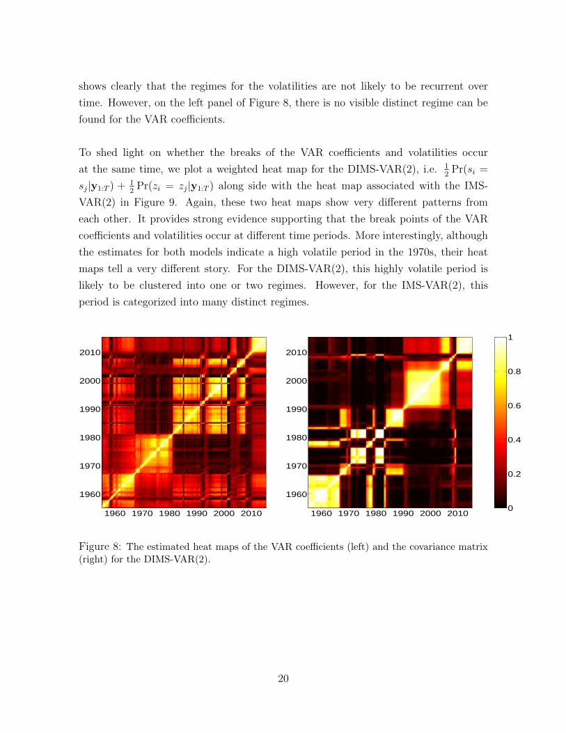
shows clearly that the regimes for the volatilities are not likely to be recurrent over

time. However, on the left panel of Figure 8, there is no visible distinct regime can be

found for the VAR coefficients.

To shed light on whether the breaks of the VAR coefficients and volatilities occur

at the same time, we plot a weighted heat map for the DIMS-VAR(2), i.e. 12

Pr(si =

sj|y1:T ) + 12

Pr(zi = zj|y1:T ) along side with the heat map associated with the IMS-

VAR(2) in Figure 9. Again, these two heat maps show very different patterns from

each other. It provides strong evidence supporting that the break points of the VAR

coefficients and volatilities occur at different time periods. More interestingly, although

the estimates for both models indicate a high volatile period in the 1970s, their heat

maps tell a very different story. For the DIMS-VAR(2), this highly volatile period is

likely to be clustered into one or two regimes. However, for the IMS-VAR(2), this

period is categorized into many distinct regimes.

1960 1970 1980 1990 2000 2010

1960

1970

1980

1990

2000

2010

1960 1970 1980 1990 2000 2010

1960

1970

1980

1990

2000

2010

0

0.2

0.4

0.6

0.8

1

Figure 8: The estimated heat maps of the VAR coefficients (left) and the covariance matrix(right) for the DIMS-VAR(2).

20

1960 1970 1980 1990 2000 2010

1960

1970

1980

1990

2000

2010

1960 1970 1980 1990 2000 2010

1960

1970

1980

1990

2000

2010

0

0.2

0.4

0.6

0.8

1

Figure 9: The estimated weighted heat map for the DIHM-VAR(2) (left) and the estimatedheat map for the IMS-VAR(2) (right).

A few implications can be drawn from the results reported in this section. The esti-

mation results show substantial time-variation in the parameters of both models. The

main difference between the DIMS-VAR(2) and IMS-VAR(2) appears in the estimates

of volatilities rather than the VAR coefficients. More importantly, it is evident that

the breaks for the VAR coefficients and volatilities are not likely to occur at the same

time. In addition, it is worth noting that even though some of the estimated parame-

ters for both models seem to share some similarities, but the latent dynamics, as shown

in Figure 6 - Figure 9, are quite different. As various types of IMS model are likely

to possess different features, it is important to investigate which type of these models

has better forecasting performance. To this end, we proceed by conducting a formal

recursive out-of-sample forecasting exercise in the next section.

5.3 Forecasting Results

This section performs a recursive out-of-sample forecasting exercise to evaluate the

performance of the models discussed in section 3. We evaluate the iterated h-step-

ahead forecasts of each model with h = 1 (one quarter), h = 2 (two quarters), h = 4

(one year), h = 8 (two years). Our forecast evaluation period is from 1970Q1 - 2015Q1.

21

5.3.1 Forecast Metrics

Let yot+h be the observed value of yt+h and y1:t denotes the data up to time t. We

compute the h-step-ahead predictive posterior median yt+h as the point forecast for a

given model. The mean absolute forecast error (MAFE) is used to measure the accuracy

of the point forecast of a model, which is defined as

MAFE =1

T − h− t0 + 1

T−h∑t=t0

∣∣yot+h − yt+h∣∣ .

For evaluating the performance of density forecasts, we use the average log-predictive

likelihoods (ALPL) which is defined as

ALPL =1

T − h− t0 + 1

T−h∑t=t0

log pt+h(yt+h = yot+h|y1:t),

where pt+h denotes h-step-ahead predictive density function given y1:t. The log-predictive

likelihood is often used to compare forecast performance of models in Bayesian frame-

work since there is a close connection between the predictive likelihood and the marginal

likelihood. More discussions about the log-predictive likelihoods can be found in Geweke

and Amisano (2011).

To facilitate comparison, the relative scores to the benchmark models, AR(1) for the

univariate models and VAR(1) for the multivariate models, are reported. More specifi-

cally, we report the ratios of MAFEs of a given model to those of the benchmark. Hence

values less than unity indicate better point forecast performance than the benchmark.

For density forecasts, we report the difference of ALPLs of a given models to those of

the benchmark. Thus positive values indicate better density forecast performance than

the benchmark.

5.3.2 Point forecasts

Table 2 - Table 5 report the relative MAFEs and ALPLs. For each table, the forecast-

ing results for GDP inflation, GDP growth and short-term interest rate are presented

in panel a), panel b) and panel c) respectively. Our point forecast results, shown in

table 2, suggest that allowing for time-variation in model parameters is important in

improving the accuracy of point forecasts. None of models we consider produce sizable

22

and consistent improvements over DIMS-VAR(2) for forecasting GDP inflation, GDP

growth and short-term interest rate. Although the IMS-VAR(1) and IMS-VAR(2) tend

to outperform the DIMS-VAR(2) on forecasting the short term GDP inflation, these

improvements are not likely to be shared for forecasting the other variables. For ex-

ample, the IMS-VAR(2) performs relatively worse at forecasting the short-run interest

rate. It is worth noting that most of the gains in forecast accuracy appear to have

come from allowing for time-variation in the VAR coefficients. This can be shown by

comparing the performance of the DIMS-VAR(2) with C-VAR(2)-IMS. For example,

both DIMS-VAR(2) and C-VAR(2)-IMS produce almost the same forecast estimates

for all variables at various forecast horizons.

For AR models, the patterns of the point forecast results shown in Table 3 are broadly

similar to those of VARs. The DIMS-AR(2) is always among the top forecasting mod-

els. Likewise, most of the forecasting gains appear to have come from allowing for

time-variation in volatilities. Even through allowing the AR coefficients to be time-

varying tends to improve the point forecast performance, such improvements are likely

to be small. This results are in general consistent with those findings in the literature

of TVP-SV models (Clark and Ravazzolo, 2014; Chan, 2015).

Table 2: Relative MAFE; GDP Inflation (panel a)), GDP growth (panel b)), short-terminterest rate (panel c)).

a) GDP inflation b) GDP growth c) short-term interest rate

h=1 h=2 h=4 h=8 h=1 h=2 h=4 h=8 h=1 h=2 h=4 h=8

VAR(1) 1.00 1.00 1.00 1.00 1.00 1.00 1.00 1.00 1.00 1.00 1.00 1.00

VAR(2) 0.99 0.93 0.86 0.88 0.99 0.98 1.02 1.01 0.96 1.03 1.01 1.00

DIMS-VAR(1) 0.98 0.93 0.87 0.84 0.99 0.97 0.97 0.98 0.95 0.95 0.96 0.97

DIMS-VAR(2) 0.99 0.89 0.81 0.76 1.00 0.96 0.98 1.00 0.86 0.93 0.91 0.91

IMS-VAR(1) 0.96 0.93 0.87 0.86 0.99 0.97 0.98 1.01 1.01 1.04 0.99 1.01

IMS-VAR(2) 0.95 0.88 0.80 0.79 1.00 0.97 1.02 1.01 0.97 1.07 1.01 1.00

C-VAR(1)-IMS 0.99 0.97 0.95 0.93 0.99 0.98 0.98 0.99 0.98 0.96 0.97 0.94

C-VAR(2)-IMS 0.98 0.89 0.81 0.77 0.99 0.97 0.98 1.00 0.86 0.92 0.91 0.90

23

Table 3: Relative MAFE; GDP Inflation (panel a)), GDP growth (panel b)), short-terminterest rate (panel c)).

a) GDP inflation b) GDP growth c) short-term interest rate

h=1 h=2 h=4 h=8 h=1 h=2 h=4 h=8 h=1 h=2 h=4 h=8

AR(1) 1.00 1.00 1.00 1.00 1.00 1.00 1.00 1.00 1.00 1.00 1.00 1.00

AR(2) 0.98 0.95 0.95 0.96 1.00 1.00 0.99 1.00 0.90 1.03 1.00 0.99

DIMS-AR(1) 0.99 0.96 0.92 0.89 1.01 1.00 1.00 1.01 0.87 0.93 0.96 0.99

DIMS-AR(2) 0.97 0.92 0.90 0.88 1.00 1.00 0.99 1.01 0.82 0.95 0.95 0.96

IMS-AR(1) 0.98 0.95 0.92 0.86 1.01 1.00 1.00 1.01 0.88 0.95 0.93 0.95

IMS-AR(2) 0.97 0.92 0.90 0.87 1.00 0.97 1.02 1.01 0.83 0.96 0.93 0.91

C-AR(1)-IMS 0.99 0.97 0.94 0.92 1.01 1.00 1.00 1.01 0.96 0.97 0.99 0.99

C-AR(2)-IMS 0.97 0.92 0.92 0.90 1.00 1.00 0.99 1.01 0.82 0.94 0.95 0.97

5.3.3 Density forecasts

We report the results of density forecasts in Table 4 and Table 5. For both VAR and

AR models, it is apparent that models allowing for time-variation in parameters, either

in the VAR coefficients or volatilities, substantially outperform the benchmarks at all

forecast horizons. Among the VAR models with infinite hidden Markov component(s),

the DIMS-VAR(2) performs the best at all horizons in forecasting GDP inflation, GDP

growth and short-term interest rate. With AR models, the patterns are mostly the same

as those of VAR models. Except in the case of forecasting short-term interest rate, the

DIMS-AR(2) and IMS-AR(2) perform quite similarly at short horizons, however the

IMS-AR(2) tends to be forecasting better than the DIMS-VAR(2) at longer horizons.

Table 4: Relative ALPL; GDP Inflation (panel a)), GDP growth (panel b)), short-terminterest rate (panel c)).

a) GDP inflation b) GDP growth c) short-term interest rate

h=1 h=2 h=4 h=8 h=1 h=2 h=4 h=8 h=1 h=2 h=4 h=8

VAR(1) 0.00 0.00 0.00 0.00 0.00 0.00 0.00 0.00 0.00 0.00 0.00 0.00

VAR(2) 0.02 0.05 0.12 0.17 -0.01 0.01 -0.02 -0.01 0.01 0.00 0.05 0.06

DIMS-VAR(1) 0.11 0.23 0.30 0.40 0.08 0.11 0.10 0.07 0.58 0.46 0.24 0.09

DIMS-VAR(2) 0.13 0.26 0.33 0.40 0.09 0.13 0.11 0.07 0.69 0.49 0.26 0.15

IMS-VAR(1) 0.12 0.20 0.26 0.35 0.04 0.05 0.04 0.03 0.39 0.32 0.16 0.11

IMS-VAR(2) 0.12 0.22 0.29 0.37 0.04 0.06 0.02 0.03 0.44 0.32 0.17 0.10

C-VAR(1)-IMS 0.10 0.18 0.19 0.24 0.08 0.11 0.10 0.06 0.47 0.35 0.16 0.09

C-VAR(2)-IMS 0.13 0.26 0.31 0.37 0.08 0.12 0.11 0.07 0.67 0.47 0.24 0.14

24

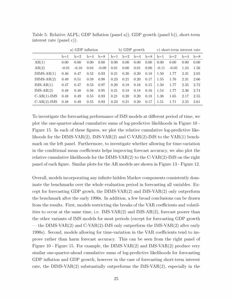
Table 5: Relative ALPL; GDP Inflation (panel a)), GDP growth (panel b)), short-terminterest rate (panel c)).

a) GDP inflation b) GDP growth c) short-term interest rate

h=1 h=2 h=4 h=8 h=1 h=2 h=4 h=8 h=1 h=2 h=4 h=8

AR(1) 0.00 0.00 0.00 0.00 0.00 0.00 0.00 0.00 0.00 0.00 0.00 0.00

AR(2) -0.01 -0.10 0.04 -0.09 0.01 0.00 0.01 0.00 -0.11 -0.05 1.24 1.56

DIMS-AR(1) 0.46 0.47 0.52 0.93 0.21 0.20 0.20 0.18 1.50 1.77 2.31 2.65

DIMS-AR(2) 0.49 0.51 0.59 0.98 0.23 0.21 0.20 0.17 1.55 1.76 2.31 2.66

IMS-AR(1) 0.47 0.47 0.53 0.97 0.20 0.18 0.16 0.15 1.50 1.77 2.35 2.72

IMS-AR(2) 0.48 0.48 0.56 0.95 0.21 0.18 0.18 0.16 1.54 1.77 2.36 2.74

C-AR(1)-IMS 0.48 0.49 0.55 0.93 0.21 0.20 0.20 0.18 1.38 1.65 2.17 2.55

C-AR(2)-IMS 0.48 0.49 0.55 0.93 0.23 0.21 0.20 0.17 1.51 1.71 2.25 2.61

To investigate the forecasting performance of IMS models at different period of time, we

plot the one-quarter-ahead cumulative sums of log-predictive likelihoods in Figure 10 -

Figure 15. In each of these figures, we plot the relative cumulative log-predictive like-

lihoods for the DIMS-VAR(2), IMS-VAR(2) and C-VAR(2)-IMS to the VAR(1) bench-

mark on the left panel. Furthermore, to investigate whether allowing for time-variation

in the conditional mean coefficients helps improving forecast accuracy, we also plot the

relative cumulative likelihoods for the DIMS-VAR(2) to the C-VAR(2)-IMS on the right

panel of each figure. Similar plots for the AR models are shown in Figure 13 - Figure 12.

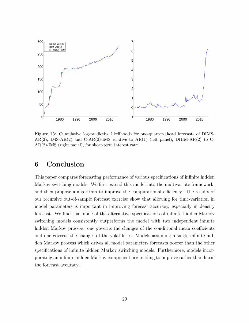
Overall, models incorporating any infinite hidden Markov components consistently dom-

inate the benchmarks over the whole evaluation period in forecasting all variables. Ex-

cept for forecasting GDP growh, the DIMS-VAR(2) and IMS-VAR(2) only outperform

the benchmark after the early 1990s. In addition, a few broad conclusions can be drawn

from the results. First, models restricting the breaks of the VAR coefficients and volatil-

ities to occur at the same time, i.e. IMS-VAR(2) and IMS-AR(2), forecast poorer than

the other variants of IMS models for most periods (except for forecasting GDP growth

— the DIMS-VAR(2) and C-VAR(2)-IMS only outperform the IMS-VAR(2) after early

1990s). Second, models allowing for time-variation in the VAR coefficients tend to im-

prove rather than harm forecast accuracy. This can be seen from the right panel of

Figure 10 - Figure 15. For example, the DIMS-VAR(2) and IMS-VAR(2) produce very

similar one-quarter-ahead cumulative sums of log-predictive likelihoods for forecasting

GDP inflation and GDP growth, however in the case of forecasting short-term interest

rate, the DIMS-VAR(2) substantially outperforms the IMS-VAR(2), especially in the

25

late 2000s.

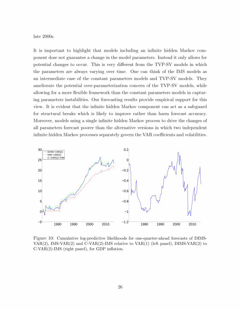
It is important to highlight that models including an infinite hidden Markov com-

ponent dose not guarantee a change in the model parameters. Instead it only allows for

potential changes to occur. This is very different from the TVP-SV models in which

the parameters are always varying over time. One can think of the IMS models as

an intermediate case of the constant parameters models and TVP-SV models. They

ameliorate the potential over-parameterization concern of the TVP-SV models, while

allowing for a more flexible framework than the constant parameters models in captur-

ing parameters instabilities. Our forecasting results provide empirical support for this

view. It is evident that the infinite hidden Markov component can act as a safeguard

for structural breaks which is likely to improve rather than harm forecast accuracy.

Moreover, models using a single infinite hidden Markov process to drive the changes of

all parameters forecast poorer than the alternative versions in which two independent

infinite hidden Markov processes separately govern the VAR coefficients and volatilities.

1980 1990 2000 2010−5

0

5

10

15

20

25

30

DIHM−VAR(2)IHM−VAR(2)C−VAR(2)−IHM

1980 1990 2000 2010−1.2

−1

−0.8

−0.6

−0.4

−0.2

0

0.2

Figure 10: Cumulative log-predictive likelihoods for one-quarter-ahead forecasts of DIMS-VAR(2), IMS-VAR(2) and C-VAR(2)-IMS relative to VAR(1) (left panel), DIMS-VAR(2) toC-VAR(2)-IMS (right panel), for GDP inflation.

26

1980 1990 2000 2010−5

0

5

10

15

20

DIHM−VAR(2)IHM−VAR(2)C−VAR(2)−IHM

1980 1990 2000 20100

0.1

0.2

0.3

0.4

0.5

0.6

0.7

Figure 11: Cumulative log-predictive likelihoods for one-quarter-ahead forecasts of DIMS-VAR(2), IMS-VAR(2) and C-VAR(2)-IMS relative to VAR(1) (left panel), DIMS-VAR(2) toC-VAR(2)-IMS ( right panel ), for GDP growth.

1980 1990 2000 20100

20

40

60

80

100

120

140

DIHM−VAR(2)IHM−VAR(2)C−VAR(2)−IHM

1980 1990 2000 2010−2

−1

0

1

2

3

4

5

Figure 12: Cumulative log-predictive likelihoods for one-quarter-ahead forecasts of DIMS-VAR(2), IMS-VAR(2) and C-VAR(2)-IMS relative to VAR(1) (left panel), DIMS-VAR(2) toC-VAR(2)-IMS (right panel), for short-term interest rate.

27

1980 1990 2000 20100

10

20

30

40

50

60

70

80

90

DIHM−AR(2)IHM−AR(2)C−AR(2)−IHM

1980 1990 2000 2010−0.5

0

0.5

1

1.5

2

2.5

Figure 13: Cumulative log-predictive likelihoods for one-quarter-ahead forecasts of DIMS-AR(2), IMS-AR(2) and C-AR(2)-IMS relative to AR(1) (left panel), DIMS-AR(2) to C-AR(2)-IMS (right panel), for GDP inflation.

1980 1990 2000 2010−5

0

5

10

15

20

25

30

35

40

45

DIHM−AR(2)IHM−AR(2)C−AR(2)−IHM

1980 1990 2000 2010−0.15

−0.1

−0.05

0

0.05

0.1

Figure 14: Cumulative log-predictive likelihoods for one-quarter-ahead forecasts of DIMS-AR(2), IMS-AR(2) and C-AR(2)-IMS relative to AR(1) (left panel), DIMS-AR(2) to C-AR(2)-IMS (right panel), for GDP growth.

28

1980 1990 2000 20100

50

100

150

200

250

300

DIHM−AR(2)IHM−AR(2)C−AR(2)−IHM

1980 1990 2000 2010−1

0

1

2

3

4

5

6

7

Figure 15: Cumulative log-predictive likelihoods for one-quarter-ahead forecasts of DIMS-AR(2), IMS-AR(2) and C-AR(2)-IMS relative to AR(1) (left panel), DIHM-AR(2) to C-AR(2)-IMS (right panel), for short-term interest rate.

6 Conclusion

This paper compares forecasting performance of various specifications of infinite hidden

Markov switching models. We first extend this model into the multivariate framework,

and then propose a algorithm to improve the computational efficiency. The results of

our recursive out-of-sample forecast exercise show that allowing for time-variation in

model parameters is important in improving forecast accuracy, especially in density

forecast. We find that none of the alternative specifications of infinite hidden Markov

switching models consistently outperforms the model with two independent infinite

hidden Markov process: one governs the changes of the conditional mean coefficients

and one governs the changes of the volatilities. Models assuming a single infinite hid-

den Markov process which drives all model parameters forecasts poorer than the other

specifications of infinite hidden Markov switching models. Furthermore, models incor-

porating an infinite hidden Markov component are tending to improve rather than harm

the forecast accuracy.

29

Appendix

In this Appendix we provide the details of the posterior sampler stated in section 4

for model DIMS-VAR(q). Posterior draws can be obtained by sequentially sampling

from Step 1. - Step 7. The sampling method is mainly based on Song (2014). We first

introduce some notation, let psi′ = (psi1, . . . , p

siL, psR

iL) and πs = (πs1, . . . , π

sL, πsR

L), where

psRiL

=∑∞

j=L+1 psij and πsR

L=∑∞

j=L+1 πsj , with similar notation applying to pzi

′ and πz.

An efficient way to obtain draws in Step 1. has been provided in the main content.

Step 2. Sample Φ

• β0 ∼ N (β0,Vβ0), where

Vβ0=(LsV

−10 + V−1

00

)−1, β0 = Vβ0

(V−10

Ls∑i=1

βi + V−100 β00)

• V−10 ∼ W(A00, a00), where

A00 =

(A−1

00 +Ls∑i=1

(βi − β0)(βi − β0)′

)−1

, a00 = a00 + Ls

• Σ0 ∼ W(Q00, b00), where

Q00 =

(Lz∑i=1

Σ−1i + Q−1

00

)−1

, b00 = b00 + Lzν0

• the conditional distribution p(ν0|Σ0,Σ1:Lz , λ00) is non-standard, a Metropolis-

Hastings step is implemented. Given the previous νo0 the current draw νc0 from

the proposal distribution q(νc0|νo0) ∼ G(χ, χ/νo0) is accepted with probability

min

1,p(νc0|Σ0,Σ1:Lz , λ00)q(νo0 |νc0)

p(νo0 |Σ0,Σ1:Lz , λ00)q(νc0|νo0)1(ν0 > n)

,

where the χ is a tuning parameter for adjusting the acceptant rate to be around

50%.

Step 3. Sample us,uz

30

• us1 ∼ U(0, πss1) and ust ∼ U(0, psst−1,st) for t = 2, . . . , T ;

• uz1 ∼ U(0, πzz1) and uzt ∼ U(0, pzzt−1,zt) for t = 2, . . . , T .

Check and expand πs and Ps as follow: If

maxpsR1L, . . . , psRLL > minus1, . . . , usT (44)

then update L as follow

3.1 draw ξ ∼ B(1, γs), and update

πs = (πs1, . . . , πsL, ξπ

sRL , (1− ξ)πsRL ) ≡ (πs1, . . . , π

sL, π

sL+1, π

sRL+1),

3.2 For i = 1, . . . , L− 1, draw ξi ∼ B(cs(1− ρs)πsL+1

, cs(1− ρs)πsRL+1

) then update

psi′ = (psi1, . . . , ξip

siL, (1− ξi)p

sRiL ) ≡ psi

′ = (psi1, . . . , psiL+1, p

sRiL+1).

3.3 Draw

psL+1′ ≡ (psi1, . . . , p

siL+1, p

sRiL+1) ∼ D(cs(1− ρs)πs1, . . . , cs(1− ρs)πsL+1 + csρs, cs(1− ρs)πsRL+1).

3.4 Set L = L+ 1.

Repeat 3.1 - 3.4 until (44) is not hold. Updating of πz and Pz are similar as those of

πs and Ps.

For Step 4. - Step 7, we only provide sampling procedure for s,πs,Ps,Hs and only

minor modification is required for sampling z,πz,Pz,Hz.

Step 4. Sample s

Given us, there are only finitely many trajectories s with non-zeros probability, i.e.

st ∈ 1, . . . , L. Hence Chib (1996) algorithm can be applied to obtain as follow

1) we first compute the conditional density of s1 given us1 which is given by

p(s1|us1,Θ,Ps) = p(s1|us1) ∝ 1(us1 < πss1) for st = 1, . . . , L;

31

2) given p(st−1|y1:t−1, us1:t−1,Θ, P s), we compute p(st|y1:t, u

s1:t,P

s,Θ) by

p(st|y1:t, us1:t,P

s,Θ)

∝p(st, ust ,y1:t|y1:t−1, us1:t−1,Θ,Ps)

=∑st−1

p(yt, |st,Θ)p(ust |st, st−1,Ps)p(st|st−1,P

s)p(st−1|y1:t−1, us1:t−1,Θ,Ps)

=p(yt|st,Θ)∑st−1

1(ust < psst−1st)p(st−1|y1:t−1, u

s1:t−1,Θ,Ps)

until we get p(sT |y1:T , us1:T ,Θ,Ps).

3) The backward sampling step can be implemented by first sample sT from p(sT |y1:T , us1:T ,Θ,P s),

then given st+1, sample st can be obtained from

p(st|st+1,us,Θ,Ps,y1:T ) ∝ p(st|y1:t,u

s,Θ,Ps)p(st+1|st, ut+1)

= p(st|y1:t,us,Θ,P s)1(ust+1 < psstst+1

).

After sampling s we find the number of active regime Ls and relabel s, Ps and Θ ac-

cordingly. Reconstruct Ps,πs by collapsing the non-active regimes and set L = Ls.

Step 5. - Step 6. Sample (πs,Ps)

To obtain sample πs and Ps we use the algorithm proposed by Song (2014). Three aux-

iliary variables (It, I′t, I′′t ) are introduced to facilitate sampling. The output (It, I

′t, I′′t )

are also used to sample Hs.

1. initialize m = (m1, . . . ,mLs) where mj = 1 if st = j and 0 otherwise. let n be

Ls × Ls zeros matrix .

2. If st 6= sl for all l = 1, . . . , t− 1, set (It, I′t, I′′t ) = (1, 1, 1);

3. else

• If st = st−1, sample (It, I′t, I′′t ) =

(0, 0, 0) ∝ nst−1st ,

(1, 0, 0) ∝ csρs,

(1, 1, 0) ∝ cs(1− ρs) mstγs+

∑j mj

,

32

• If st 6= st−1, sample (It, I′t, I′′t ) =

(0, 0, 0) ∝ nst−1st ,

(1, 0, 0) ∝ cs(1− ρs) mstγs+

∑j mj

,

4. update mst = mst + 1 if I ′t = 1. Update nst−1st = nst−1sst+ 1.

5. repeat 2. – 3. for t = 2, . . . , T .

Draw πs ∼ D(m1, . . . ,mLs , γs).

For i = 1, . . . , Ls, draw

psi′ ∼ D(cs(1− ρs)πs1 + ni1, . . . , c

s(1− ρs)πsi + csρs + nii, . . . , cs(1− ρs)πsLs + niLs , c

s(1− ρs)πsLs).

Step 7. Sample Hs

Given (I1:T , I′1:T , I

′′1:T ) obtained Step 4, we applied the method of Song (2014). Samples

from Hs can be obtained by

• Sample cs

1. we first compute ai =∑T−1

t=1 (st = i)It+1 + 1(s1 = i) and bi =∑T

t=1 1(st = i)

for i = 1, . . . , Ls;

2. sample xi ∼ B(cs, bi) for i = 1, . . . , Ls;

3. cs ∼ G(ωs +∑Ls

i=1 ai, θs −∑Ls

i=1 log(xi)).

• Sample ρs

1. compute a′ =∑T

t=2 It(1− I ′t) and b′ =∑T

t=2 ItI′t;

2. sample ρs ∼ B(fs + a′, gs + b′).

• Sample γs

1. compute a′′ =∑T

t=1 ItI′t;

2. sample x ∼ G(γs, a′′);

3. sample γs ∼ G(hs + Ls, ηs − log(x)) .

33

References

L. Bauwens, G. Koop, D. Korobilis, and J. V. Rombouts. The contribution of structuralbreak models to forecasting macroeconomic series. Journal of Applied Econometrics,2014.

L. Bauwens, J.-F. Carpantier, A. Dufays, et al. Autoregressive moving average infinitehidden markov-switching models. Journal of Business and Economic Statistics,(forecoming), 2015.

J. C. Chan. Moving average stochastic volatility models with application to inflationforecast. Journal of Econometrics, 176(2):162–172, 2013.

J. C. Chan. Large Bayesian VARs: A flexible kronecker error covariance structure.Available at SSRN 2688342, 2015.

J. C. Chan and E. Eisenstat. Bayesian model comparison for time-varying parameterVARs with stochastic volatility. Technical report, Centre for Applied MacroeconomicAnalysis, Crawford School of Public Policy, The Australian National University, 2015.

J. C. Chan and I. Jeliazkov. Efficient simulation and integrated likelihood estimation instate space models. International Journal of Mathematical Modelling and NumericalOptimisation, 1(1-2):101–120, 2009.

S. Chib. Calculating posterior distributions and modal estimates in Markov mixturemodels. Journal of Econometrics, 75(1):79–97, 1996.

S. Chib. Estimation and comparison of multiple change-point models. Journal ofEconometrics, 86(2):221–241, 1998.

T. E. Clark. Real-time density forecasts from Bayesian vector autoregressions withstochastic volatility. Journal of Business and Economic Statistics, 29(3), 2011.

T. E. Clark and F. Ravazzolo. Macroeconomic forecasting performance under alterna-tive specifications of time-varying volatility. Journal of Applied Econometrics, 2014.

T. Cogley and T. J. Sargent. Evolving post-World War II US inflation dynamics. InNBER Macroeconomics Annual 2001, Volume 16, pages 331–388. MIT Press, 2002.

T. Cogley and T. J. Sargent. Drifts and volatilities: monetary policies and outcomesin the post WWII US. Review of Economic Dynamics, 8(2):262–302, 2005.

A. D’Agostino, L. Gambetti, and D. Giannone. Macroeconomic forecasting and struc-tural change. Journal of Applied Econometrics, 28(1):82–101, 2013.

T. S. Ferguson. A Bayesian analysis of some nonparametric problems. The Annals ofStatistics, pages 209–230, 1973.

34

E. B. Fox, E. B. Sudderth, M. I. Jordan, and A. S. Willsky. A sticky HDP-HMM withapplication to speaker diarization. The Annals of Applied Statistics, pages 1020–1056,2011.

J. Geweke. Interpretation and inference in mixture models: Simple MCMC works.Computational Statistics and Data Analysis, 51(7):3529–3550, 2007.

J. Geweke and G. Amisano. Hierarchical Markov normal mixture models with ap-plications to financial asset returns. Journal of Applied Econometrics, 26(1):1–29,2011.

J. Geweke and Y. Jiang. Inference and prediction in a multiple-structural-break model.Journal of Econometrics, 163(2):172–185, 2011.

P. Giordani and R. Kohn. Efficient Bayesian inference for multiple change-point andmixture innovation models. Journal of Business and Economic Statistics, 2012.

K. Hubrich and R. J. Tetlow. Financial stress and economic dynamics: The transmissionof crises. Journal of Monetary Economics, 70:100–115, 2015.

I. Jeliazkov. Specification and inference in nonparametric additive regression. 2008.

M. J. Jensen and J. M. Maheu. Estimating a semiparametric asymmetric stochasticvolatility model with a dirichlet process mixture. Journal of Econometrics, 178:523–538, 2014.

M. Jochmann. Modeling US inflation dynamics: A Bayesian nonparametric approach.Econometric Reviews, 34(5):537–558, 2015.

M. Jochmann and G. Koop. Regime-switching cointegration. Studies in NonlinearDynamics and Econometrics, 19(1):35–48, 2015.

C.-J. Kim, C. R. Nelson, and J. Piger. The less-volatile US economy: A Bayesianinvestigation of timing, breadth, and potential explanations. Journal of Businessand Economic Statistics, 22(1):80–93, 2004.

G. Koop and S. M. Potter. Estimation and forecasting in models with multiple breaks.The Review of Economic Studies, 74(3):763–789, 2007.

G. Koop, R. Leon-Gonzalez, and R. W. Strachan. On the evolution of the monetarypolicy transmission mechanism. Journal of Economic Dynamics and Control, 33(4):997–1017, 2009.

Y. Liu and J. Morley. Structural evolution of the postwar US economy. Journal ofEconomic Dynamics and Control, 42:50–68, 2014.

J. M. Maheu and Q. Yang. An infinite hidden Markov model for short-term InterestRates. 2015.

35

G. E. Primiceri. Time varying structural vector autoregressions and monetary policy.The Review of Economic Studies, 72(3):821–852, 2005.

J. Sethuraman. A constructive definition of dirichlet priors. Statistica Sinica, 4:639–650,1994.

C. A. Sims and T. Zha. Were there regime switches in US monetary policy? TheAmerican Economic Review, pages 54–81, 2006.

Y. Song. Modelling regime switching and structural breaks with an infinite hiddenMarkov model. Journal of Applied Econometrics, 29(5):825–842, 2014.

J. H. Stock and M. W. Watson. Evidence on structural instability in macroeconomictime series relations. Journal of Business and Economic Statistics, 14(1):11–30, 1996.

J. H. Stock and M. W. Watson. Why has US inflation become harder to forecast?Journal of Money, Credit and banking, 39(s1):3–33, 2007.

Y. W. Teh, M. I. Jordan, M. J. Beal, and D. M. Blei. Hierarchical dirichlet processes.Journal of the American Statistical Association, 101(476), 2006.

J. Van Gael, Y. Saatci, Y. W. Teh, and Z. Ghahramani. Beam sampling for theinfinite hidden Markov model. In Proceedings of the 25th International Conferenceon Machine Learning, pages 1088–1095. ACM, 2008.

36