The Beveridge Curve - Welcome to LSE Research Online - LSE...
61
Abstract This paper is an empirical analysis of unemployment patterns in the OECD countries from the 1960s to the 1990s, looking at the Beveridge Curves, real wages as well as unemployment directly. Our results indicate the following. First, the Beveridge Curves of all the countries except Norway and Sweden shifted to the right from the 1960s to the early/mid 1980s. At this point, the countries divide into two distinct groups. Those whose Beveridge Curves continued to shift out and those where the y started to shift back. Second, we find evidence that these movements in the Beveridge Curves may be partly explained by changes in labour market institutions, particularly those which are important for search and matching efficiency. Third, labour market institutions impact on real labour costs in a fashion which is broadly consistent with their impact on unemployment. Finally, broad movements in unemployment across the OECD can be explained by shifts in labour market institutions although this explanation relies on high levels of endogenous persistence as reflected in a lagged dependent variable coefficient of around 0.85. JEL Numbers: E240, J300. Keywords: Beveridge Curve, labour market rigidities, unemployment rates, wage determination This paper was produced as part of the Centre’s Labour Markets Programme
-
Upload
duongthuan -
Category
Documents
-
view
229 -
download
0
Transcript of The Beveridge Curve - Welcome to LSE Research Online - LSE...

Abstract
This paper is an empirical analysis of unemployment patterns in the OECD countries from
the 1960s to the 1990s, looking at the Beveridge Curves, real wages as well as unemployment
directly.
Our results indicate the following. First, the Beveridge Curves of all the countries
except Norway and Sweden shifted to the right from the 1960s to the early/mid 1980s. At
this point, the countries divide into two distinct groups. Those whose Beveridge Curves
continued to shift out and those where they started to shift back. Second, we find evidence
that these movements in the Beveridge Curves may be partly explained by changes in labour
market institutions, particularly those which are important for search and matching
efficiency. Third, labour market institutions impact on real labour costs in a fashion which is
broadly consistent with their impact on unemployment. Finally, broad movements in
unemployment across the OECD can be explained by shifts in labour market institutions
although this explanation relies on high levels of endogenous persistence as reflected in a
lagged dependent variable coefficient of around 0.85.
JEL Numbers: E240, J300.
Keywords: Beveridge Curve, labour market rigidities, unemployment rates, wage determination
This paper was produced as part of the Centre’s
Labour Markets Programme

The Beveridge Curve, Unemployment and Wages in
the OECD from the 1960s to the 1990s
Stephen Nickell, Luca Nunziata,
Wolfgang Ochel and Glenda Quintini
July 2002

Published by Centre for Economic Performance London School of Economics and Political Science Houghton Street London WC2A 2AE Stephen Nickell, Luca Nunziata, Wolfgang Ochel and Glenda Quintini, submitted May 2001. Updated October 2001. ISBN 0 7530 1490 4 Individual copy price: £5

The Beveridge Curve, Unemployment and Wages in the OECD from the 1960s to the 1990s
Stephen Nickell, Luca Nunziata,
Wolfgang Ochel and Glenda Quintini
1. Introduction 1
2. Theoretical Background 2
3. Factors Influencing Unemployment in the OECD, 1960s-1990s 6
4. The Basic Empirical Strategy 10
5. Shifts in the Beveridge Curve, Real Wages and Unemployment 12
6. Summary and Conclusions 18
Endnotes 20
Tables 25
Figures 40
Data Appendix 46
References 50
The Centre for Economic Performance is financed by the Economic and Social Research Council

Acknowledgements
We would like to thank the ESRC Centre for Economic Performance, CES ifo, Munich and
the Bank of England External MPC Unit for help in the production of this paper.
We are also grateful to the Leverhulme Trust Programme on the Labour Market
Consequences of Structural and Technological Change and CESifo, Munich for financial
assistance. Finally our thanks are due to Michèle Belot, Olivier Blanchard, Guiseppe
Nicoletti, Andrew Oswald, Jan Van Ours and Justin Wolfers for help with our data, as well as
useful comments on an earlier draft.
Stephen Nickell is a member of the Monetary Policy Committee, Bank of England
([email protected] ) and the Centre for Economic Performance, London
School of Economics ([email protected] ). Luca Nunziata is at Nuffield College, Oxford
([email protected]). Wolfgang Ochel is a member of the Ifo Institute for
Economic Research in Munich ([email protected]). Glenda Quintini is contactable at Credit
Suisse First Boston, One Cabot Square, London E14 4QJ.

1. Introduction
“The main message transmitted by the Beveridge curves for France and Germany goes squarely against the cliché that high and persistent unemployment is entirely or mainly a matter of worsening functioning of the labour market. It is precisely in France and Germany that there is no sign of a major unfavourable shift of the Beveridge curve during the period of rising unemployment.” (R. Solow, 2000, p.5)
“Explanations (of high unemployment) based solely on institutions also run however into a major empirical problem: many of these institutions were already present when unemployment was low ………. Thus, while labour market institutions can potentially explain cross country differences to-day, they do not appear able to explain the general evolution of unemployment over time.” (O.Blanchard and J.Wolfers, 2000, p.C2)
“Despite conventional wisdom, high unemployment does not appear to be primarily the result of things like overly generous benefits, trade union power, taxes, or wage ‘inflexibility’.” (A.Oswald, 1997, p.1)
It is widely accepted, not least because of the pioneering work of Phelps, that labour market
rigidities are an important part of the explanation for the high levels of unemployment which
are still to be found in many OECD countries. However, this view is not universally accepted
and there remain serious problems as the above quotations indicate. One such problem,
emphasised by Blanchard and Wolfers (2000), may be summarised as follows: labour market
rigidities cannot explain why European unemployment is so much higher than US
unemployment because the institutions generating these rigidities were much the same in the
1960s as they are today and in the 1960s, unemployment was much higher in the United
States than in Europe.
Before going any further, it is worth looking at the actual numbers reported in Table
1. This confirms that the United States indeed had the highest unemployment in the OECD
in the early 1960s but the picture today is not quite as clear-cut as is commonly thought. In
fact, many of the smaller European countries have unemployment rates which are in the same
ball park as that in the United States although none have reached the extraordinarily low
levels ruling in the early 1960s.

2
Our purpose is what follows is to shed some further light on the patterns of
unemployment seen in the OECD from the 1960s to the 1990s. In particular, we want to
focus on the problem noted above and, more generally, on the challenges set out in our
introductory quotes. Our aim is to see how far it is possible to defend the proposition that the
dramatic long term shifts in unemployment seen in the OECD countries over the period from
the 1960s to the 1990s can be explained simply by changes in labour market institutions in
the same period. The institutions concerned will be the usual suspects set out in the Oswald
(1997) quote, namely generous benefits, trade union power, taxes and wage “inflexibility”.
Our strategy is very straightforward. We analyse shifts in the Beveridge Curve, real wages
and unemployment over time and explain these shifts by institutional changes and
macroeconomic shocks. We focus on the times series variation in the data and eschew the
extensive use of interactions which differentiates our analysis from that of Blanchard and
Wolfers (2000), Belot and Van Ours (2000) and Fitoussi et al. (2000). Are we successful in
our main aim? We feel that we probably deserve a B grade. The story that emerges is
reasonably consistent but not totally decisive. Experts on individual countries would
probably feel that we had not produced wholly persuasive explanations of the unemployment
shifts in each country and we make no attempt to provide a country by country story.
Furthermore, we have not faced up to the problem of the endogeneity of the institutional
shifts. In certain cases this may be important but, overall, we do not feel this problem
seriously distorts our results. In any event, the absence of suitable instruments ensures that
we are unable to deal with the issue.
The remainder of the paper is set out as follows. In the next section we briefly discuss
our theoretical framework and then, in Section 3, we look at the various institutions and
discuss our data. In Section 4 we lay out our empirical strategy and in Section 5 we present
our results. We finish with a summary and conclusions.
2. Theoretical Background There are innumerable detailed theories of unemployment in the long run. These may be
divided into two broad groups, those based on flow models and those based on stock models.
Pissarides (1990) and Mortensen and Pissarides (1999) provide good surveys of the former
model type. Blanchard and Katz (1997) presents a general template for the latter models.
Fundamentally, all the models have the same broad implications. First, unemployment in the

3
short-run and in the long-run is determined by real demand. Second, over the long term, real
demand and unemployment generally tend towards the level consistent with stable inflation.
This we term the equilibrium level. Various possible mechanisms may be at work here. For
example, many OECD countries now set monetary policy on the basis of an inflation target
which naturally moves real demand and unemployment towards the equilibrium defined
above1. Third, the equilibrium level of unemployment is affected first, by any variable which
influences the ease with which unemployed individuals can be matched to available job
vacancies, and second, by any variable which tends to raise wages in a direct fashion despite
excess supply in the labour market. There may be variables common to both sets. Finally,
both groups of variables will tend to impact on real wages in the same direction as they
influence equilibrium unemployment, essentially because equilibrium labour demand, which
is negatively related to wages, has to move in the opposite direction to equilibrium
unemployment.
Before going on to consider these variables in more detail, it is worth noting that the
first group of variables mentioned above will tend to impact on the position of the Beveridge
Curve (UV locus), whereas the second will not do so in any direct fashion. However, this
division is not quite as clear cut as it might appear at first sight (see below). What we can
say, nevertheless is that any variable which shifts the Beveridge Curve to the right will
increase equilibrium unemployment. So a shift of the Beveridge Curve is a sufficient but not
necessary sign that equilibrium unemployment has changed.
We turn now to consider a series of variables which we might expect to influence
equilibrium unemployment either because of their impact on the effectiveness with which the
unemployed are matched to available jobs or because of their direct effect on wages. The
unemployment benefit system directly affects the readiness of the unemployed to fill
vacancies. Aspects of the system which are clearly important are the level of benefits, their
coverage, the length of time for which they are available and the strictness with which the
system is operated. Related to unemployment benefits is the availability of other resources to
those without jobs. These include the returns on non-human wealth which may be increasing
in the real interest rate. (See Phelps, 1994, for an extensive discussion.) Employment
protection laws may tend to make firms more cautious about filling vacancies which slows
the speed at which the unemployed move into work. This obviously reduces the efficiency of
job matching. However, the mechanism here is not clear-cut. For example, the introduction
of employment laws often leads to an increased professionalisation of the personnel function
within firms, as was the case in Britain in the 1970s (see Daniel and Stilgoe, 1978). This can

4
increase the efficiency of job matching. So, in terms of outflows from unemployment, the
impact of employment protection laws can go either way. By contrast, it seems clear that
such laws will tend to reduce involuntary separations and hence lower inflows into
unemployment2. So the overall impact on the Beveridge Curve is an empirical question.
Furthermore, employment law may also have a direct impact on pay since it raises the job
security of existing employees encouraging them to demand higher pay increases.
Anything which makes it easier to match the unemployed to the available vacancies
will shift the Beveridge Curve to the left and reduce equilibrium unemployment. Factors
which operate in this way include the reduction of barriers to mobility which may be
geographical or occupational. Furthermore numerous government policies are concerned to
increase the ability and willingness of the unemployed to take jobs. These are grouped under
the heading of active labour market policies.
Turning now to those factors which have a direct impact on wages, the obvious place
to start is the institutional structure of wage determination. Within every country there is a
variety of structures. In some sectors wages are determined more of less competitively but in
others wages are bargained between employers and trade unions at the level of the
establishment, firm or even industry. The overall outcome depends on union power in wage
bargains, union coverage and the degree of co-ordination of wage bargains. Generally,
greater union power and coverage can be expected to exert upward pressure on wages, hence
raising equilibrium unemployment, but this can be offset if union wage setting across the
economy is co-ordinated. Superficially it may be argued that wage setting institutions impact
directly on wages without influencing the efficiency of job matching or the separation rate
into unemployment. That is, without influencing the position of the Beveridge Curve.
However, if we use a model of the Beveridge Curve which endogenises the rate of separation
into unemployment or the rate of job destruction (see Mortensen and Pissarides, 1994, for
example), this no longer applies. For example, if union power raises the share of the
matching surplus going to wages, this will tend to raise the rate of job destruction and shift
the Beveridge Curve to the right. The same thing will also happen if factors such as the co-
ordination of wage bargaining reduce the extent to which wages at the firm level can
fluctuate to offset idiosyncratic shocks and stabilise employment at the firm level. So while
co-ordination can reduce overall wage pressure, which tends to lower equilibrium
unemployment, it may raise the rate of idiosyncratic job shifts which will tend to shift the
Beveridge Curve to the right and have an offsetting effect.
5
The final group of variables which directly impacts on wages falls under the heading
of real wage resistance. The idea here is that workers attempt to sustain recent rates of real
wage growth when the rate consistent with stable employment shifts unexpectedly. For
example, if there is an adverse shift in the terms of trade, real consumption wages must fall if
employment is not to decline. If workers persist in attempting to bargain for rates of real
wage growth which take no account of the movement in the terms of trade, this will tend to
raise unemployment. Exactly the same argument applies if there is an unexpected fall in
trend productivity growth or an increase in labour taxes. For example, if labour taxes
(payroll tax rates plus income tax rates plus consumption tax rates) go up, the real post-tax
consumption wage must fall if real labour costs per employee facing firms are not to rise.
Any resistance to this fall will lead to a rise in unemployment. This argument suggests that
increases in real import prices, falls in trend productivity growth or rises in the labour tax rate
may lead to a temporary increase in unemployment.
However, some argue that these effects can be permanent. For example, Mortensen
and Pissarides (1999) use their standard flow model of equilibrium unemployment to analyse
various economic policies including changes in payroll taxes. And they find enormous
effects. For example, in one simulation, with a benefit replacement ratio of 0.4, a rise in the
payroll tax rate from 15 to 25 percent is enough to raise equilibrium unemployment
permanently by over 6 percentage points. The reason why labour taxes have a big impact in
this case is because Mortensen and Pissarides introduce into their model a value of leisure
which is independent of the consumption wage. This fixing of an important element of the
individual reservation wage implies that labour supply and willingness to work will increase
permanently if the real consumption wage goes up. This will induce permanent reductions in
equilibrium unemployment if labour taxes fall or productivity rises. Ultimately this is an
empirical question but it may be argued that in a satisfactory model, the value of leisure, and
the individual reservation wage more generally, should, in the long run, move proportionally
to the consumption wage and the general level of productivity. If this adjustment is made in
the Mortensen and Pissarides model, the impact of payroll taxes on equilibrium
unemployment disappears.
To summarise, the variables which we might expect to influence equilibrium
unemployment include the unemployment benefit system, the real interest rate, employment
protection laws, barriers to labour mobility, active labour market policies, union structures
and the extent of co-ordination in wage bargaining, labour taxes, terms of trade changes and
shifts in trend productivity growth. Given the inverse relationship between the equilibrium

6
unemployment and equilibrium employment, the impact of any of the above variables on
unemployment should be reflected by a ceteris paribus impact in the same direction on real
wages which are, of course, inversely related to employment.
3. Factors Influencing Unemployment in the OECD, 1960s-1990s
Our purpose is to investigate the effect of changes in labour market “institutions” on the
Beveridge Curve, real wages and equilibrium unemployment in the OECD from the 1960s to
the 1990s. In order to undertake this task, we require long time series for the appropriate
countries. In this section, we describe the information we possess and also indicate the gaps
in our knowledge. The variables we consider relate, in turn, to the benefit system, the system
of wage determination, employment protection, labour taxes and barriers to labour mobility.
The Unemployment Benefit System
There are four aspects of the unemployment benefit system for which there are good
theoretical and empirical reasons to believe that they will influence equilibrium
unemployment. These are, in turn, the level of benefits3, the duration of entitlement4, the
coverage of the system5 and the strictness with which the system is operated6. Of these, only
the first two are available as time series for the OECD countries. The OECD has collected
systematic data on the unemployment benefit replacement ratio for three different family
types (single, with dependent spouse, with spouse at work) in three different duration
categories (1st year, 2nd and 3rd years, 4th and 5th years) from 1961 to 1995 (every other year).
(See OECD, 1994, Table 8.1 for the 1991 data). From this we derive a measure of the benefit
replacement ratio, equal to the average over family types in the 1st year duration category and
a measure of benefit duration equal to [0.6 (2nd and 3rd year replacement ratio) + 0.4 (4th and
5th year replacement ratio)] ÷ (1st year replacement ratio). So our measure of benefit duration
is the level of benefit in the later years of the spell normalised on the benefit in the first year
of the spell. A summary of these data is presented in Tables 2 and 3.
It is unfortunate that we have no comprehensive time series data on the coverage of
the system or on the strictness with which it is administered. This is particularly true in the
case of the latter because the evidence we possess appears to indicate that this is of crucial
importance in determining the extent to which a generous level of benefit will actually

7
influence unemployment. For example, Denmark, which has very generous unemployment
benefits (see Tables 2 and 3), totally reformed the operation of its benefit system through the
1990s with a view to tightening the criteria for benefit receipt and the enforcement of these
criteria via a comprehensive system of sanctions. The Danish Ministry of Labour is
convinced that this process has played a major role in allowing Danish unemployment to fall
dramatically since the early 1990s without generating inflationary pressure (see Danish
Ministry of Finance, 1999, Chapter 2).
A further aspect of the structure of the benefit system for which we do not have
detailed data back to the 1960s are those policies grouped under the heading of active labour
market policies (ALMP). The purpose of these is to provide active assistance to the
unemployed which will improve their chances of obtaining work. Multi-country studies
basically using cross section information indicate that ALMPs do have a negative impact on
unemployment (e.g. Scarpetta, 1996; Nickell, 1997; Elmeskov et al., 1998). This broad brush
evidence is backed up by numbers of microeconometric studies (see Katz, 1998 or Martin,
2000 for useful surveys) which show that under some circumstances, active labour market
policies are effective. In particular, job search assistance tends to have consistently positive
outcomes but other types of measure such as employment subsidies and labour market
training must be well designed if they are to have a significant impact (see again Martin,
2000, for a detailed analysis).
Systems of Wage Determination
In most countries in the OECD, the majority of workers have their wages set by collective
bargaining between employers and trade unions at the plant, firm, industry or aggregate level.
This is important for our purposes because there is some evidence that trade union power in
wage setting has a significant impact on unemployment7. Unfortunately, we do not have
complete data on collective bargaining coverage (the proportion of employees covered by
collective agreements) but the data presented in Table 4 give a reasonable picture. Across
most of Continental Europe, including
Scandinavia but excluding Switzerland coverage is both high and stable. As we shall
see, this is either because most people belong to trade unions or because union agreements
are extended by law to cover non-members in the same sector. In Switzerland and in the
OECD countries outside Continental Europe and Scandinavia, coverage is generally much

8
lower with the exception of Australia. In the UK, the US and New Zealand, coverage has
declined with the fall in union density, there being no extension laws.
In Table 5, we present the percentage of employees who are union members. Across
most of Scandinavia, membership tends to be high. By contrast, in much of Continental
Europe and in Australia, union density tends to be less than 50 percent and is gradually
declining. In these countries there is, consequently, a wide and widening gap between
density and coverage which it is the job of the extension laws to fill. This situation is at its
most stark in France, which has the lowest union density in the OECD at around 10 percent,
but one of the highest levels of coverage (around 95 percent). Outside these regions, both
density and coverage tend to be relatively low and both are declining at greater or lesser rates.
The absence of complete coverage data means that we have to rely on the density variable to
capture the impact of unionisation on unemployment. As should be clear, this is only half the
story, so we must treat any results we find in this area with some caution.
The other aspect of wage bargaining which appears to have a significant impact on
wages and unemployment is the extent to which bargaining is co-ordinated8,9. Roughly
speaking, the evidence suggests that if bargaining is highly co-ordinated, this will completely
offset the adverse effects of unionism on employment (see Nickell and Layard, 1999, for
example). Co-ordination refers to mechanisms whereby the aggregate employment
implications of wage determination are taken into account when wage bargains are struck.
This may be achieved if wage bargaining is highly centralised, as in Austria, or if there are
institutions, such as employers’ federations, which can assist bargainers to act in concert even
when bargaining itself ostensibly occurs at the level of the firm or industry, as in Germany or
Japan (see Soskice, 1991). It is worth noting that co-ordination is not, therefore, the same as
centralisation which refers simply to the level at which bargaining takes place (plant, firm,
industry or economy-wide). In Table 6, we present co-ordination indices for the OECD from
the 1960s. The first index (co-ord 1) basically ignores transient changes whereas the second
(co-ord 2) tries to capture the various detailed nuances of the variations in the institutional
structure. Notable changes are the increases in co-ordination in Ireland and the Netherlands
towards the end of the period and the declines in co-ordination in Australia, New Zealand and
Sweden. Co-ordination also declines in the UK over the same period but this simply reflects
the sharp decline of unionism overall.

9
Employment Protection
Employment protection laws are thought by many to be a key factor in generating labour
market inflexibility. Despite this, evidence that they have a decisive impact on overall rates
of unemployment is mixed, at best10. In Table 7, we present details of an employment
protection index for the OECD countries. Features to note are the wide variation in the index
across countries and the fact that, in some countries, the basic legislation was not introduced
until the 1970s.
Labour Taxes
The important taxes here are those that form part of the wedge between the real product wage
(labour costs per employee normalised on the output price) and the real consumption wage
(after tax pay normalised on the consumer price index). These are payroll taxes, income
taxes and consumption taxes. Their combined impact on unemployment remains a subject of
some debate despite the large number of empirical investigations. Indeed some studies
indicate that employment taxes have no long run impact on unemployment whatever whereas
others present results which imply that they can explain more or less all the rise in
unemployment in most countries during the 1960-1985 period11. In Table 8 we present the
total tax rate on labour for the OECD countries. All countries exhibit a substantial increase
over the period from the 1960s to the 1990s although there are wide variations across
countries. These mainly reflect the extent to which health, higher education and pensions are
publicly provided along with the all- round generosity of the social security system.
Barriers to Labour Mobility
Oswald (1997) proposes that barriers to geographical mobility, as reflected in the rate of
owner occupation of the housing stock, play a key role in determining unemployment. He
finds that changes in unemployment are positively correlated with changes in owner
occupation rates across countries, US states and UK regions. He also presents UK evidence
that owner occupation represents a significant mobility barrier relative to private renting.
However, Gregg et al. (2000) find that while unemployment is significantly negatively
related to unemployment both across UK regions and across time in a regional fixed effects
model, this relationship becomes significantly positive once other relevant regional

10
characteristics are included. We propose to include owner occupation as a variable in our
investigation and the data are shown in Table 9. It must, however, be born in mind that these
data are heavily interpolated, so the results should be treated with caution.
4. The Basic Empirical Strategy
Our aim is to explain the different patterns of unemployment exhibited across the OECD in
the period from the 1960s to the 1990s. Our approach is to see how far we can get with a
very simple empirical model. We have already discussed those factors which can be
expected to influence equilibrium unemployment in the long run. Then, since we are, in
practice, going to explain actual unemployment, we must also include in our model those
factors which might explain the short-run deviations of unemployment from its equilibrium
level. Following the discussion in Hoon and Phelps (1992) or Phelps (1994) these factors
include aggregate demand shocks, productivity shocks and wage shocks. More specifically,
we include the following (see Data Appendix for details):
i) money supply shocks, specifically changes in the rate of growth of the nominal
money stock (i.e. the second difference of the log money supply);
ii) productivity shocks, measured by changes in TFP growth or deviations of TFP growth
from trend;
iii) labour demand shocks, measured by the residuals from a simple labour demand
model;
iv) real import price shocks, measured by proportional changes in real import prices
weighted by the trade share;
v) the (ex-post) real interest rate.
With the exception of the real interest rate, these variables are genuine “shocks” in the sense
that they are typically stationary and tend to revert back to their mean quite rapidly.
Nevertheless, their impact may persist for some time, since we shall also include the lagged
dependent variable in our model to capture endogenous persistence.
Some further specific points are worth noting. The first of these is the role of
productivity shocks and real import shocks in capturing real wage resistance. As we noted in

11
Section 2, increases in real import prices or falls in trend productivity growth will lead to
temporary increases in unemployment (and in real product wages relative to trend
productivity) if real consumption wages do not adjust appropriately. Second, we include the
real interest rate because some have accorded it a significant role in the determination of
unemployment even in the long run (e.g. Phelps, 1994 or Blanchard and Wolfers, 2000).
Third, we are not simply going to look at unemployment but we shall also try and explain real
product wages (real labour costs) and shifts in the Beveridge Curve in order to see if we can
obtain a consistent picture.
Our focus is going to be on the time series variation in the cross-country data, so all
our models will include country dummies as well as time dummies. We are by no means the
first to undertake this task but what we are attempting is perhaps a little different from what
has gone before. There have been a number of previous studies but a representative picture
may be gathered from Layard et al. (1991), Chapter 9 (p.430-437), Blanchard and Wolfers
(2000), Belot and Van Ours (2000) and Fitoussi et al. (2000) all of which use panel models
with country dummies12. The first two and the last of these focus specifically on the way in
which institutions interact with variables which are either shocks or factors which may
influence unemployment in the longer term. Layard et al.(1991) present a dynamic model of
unemployment based on annual data where unemployment depends on wage pressure (simply
a dummy which takes the value one from 1970), the benefit replacement ratio, real import
price changes and monetary shocks. Their impact on unemployment depends on time
invariant institutions, with different sets of institutions affecting the degree of unemployment
persistence (captured by the lagged dependent variable), the impact of wage pressure
variables including the replacement rate and import prices, and the effect of monetary shocks.
The model generally explains the data better than individual country autoregressions with
trends.
Blanchard and Wolfers (2000) also focus on the interaction between institutional
variables and shocks, using five year averages of the data to concentrate on long-run effects.
The shock variables consist of the level of TFP growth, the real interest rate and labour
demand shifts (essentially the log of labour’s share purged of the impact of factor prices).
These shocks differ from those used here because, over the length of the sample (35 years),
they are not mean reverting. For example, annual TFP growth is as much as 3 percentage
points higher in the 1960s than in the 1990s in many countries. Interacting these shocks with
institutions fits the data well.

12
Fitoussi et al. (2000) proceed in a slightly different way. First, they interact their
baseline variables with country dummies and then investigate the cross-section relationship
between these and labour market institutions. The baseline variables include non-wage
support relative to labour productivity (income from private wealth plus social spending), the
real price of oil and two in common with Blanchard and Wolfers (2000), the real rate of
interest and productivity growth13. The explanation of unemployment shifts in all three
papers (Layard et al, 1991; Blanchard and Wolfers, 2000; Fitoussi et al., 2000) has the same
fundamental structure. They depend on long-run changes in a set of baseline variables, with
the impact of these long-run shifts being much bigger and longer lasting in some countries
than others because of institutional differences. The extent to which these explanations are
persuasive depends on whether the stories associated with the baseline variables are
convincing. For example, the notion that a fall in trend productivity growth or a rise in the
real price of oil leads to a permanent rise in the equilibrium unemployment rate is one which
many find unappealing.
Belot and van Ours (2000) is closer in spirit to our analysis. They rely on
“institutional” shifts to explain the changes in unemployment. They typically include large
numbers of interactions between institutions, many of which are highly significant (see, for
example, their Table 6, equation 8). This has a sound theoretical foundation (see Coe and
Snower, 1997, for example) and undoubtedly helps greatly with the explanatory power of the
model. The model is, however, static so that the within country persistence of unemployment
is excluded.
In the light of what has gone before, we propose to see how much the institutional
information described in Section 3 can explain if it is taken more or less straight. That is with
only a minimum of interactions and with the addition of some mean reverting shocks. The
results of our investigation are presented next.
5. Shifts in the Beveridge Curve, Real Wages and Unemployment
In this section we set out our results concerning first, shifts in the Beveridge Curve, second,
real labour costs and third, unemployment. We shall also briefly look at employment rates
for the benefit of those who prefer to use this measure14.

13
Shifts in the Beveridge Curve
In Figure 1 we present plots of the unemployment rate against the vacancy rate for all our
countries except Ireland and Italy, where vacancy data are unavailable. For completeness, in
France we also show a plot using a labour shortage index in place of the vacancy rate.
Recall that if the economy fluctuates with a stationary Beveridge Curve, we expect to
see the uv dots cycling anti-clockwise around a fixed downward sloping line. If the steady-
state Beveridge Curve is also moving then these cycles will shift either rightwards or
leftwards. Furthermore if the steady state curve is moving very fast, the cycles will not be
clearly visible. By eye-balling the pictures, two points stand out. First, for every country
except Norway and Sweden, the Beveridge Curve shifted to the right from the 1960s to the
mid- 1980s. Of course, the distance moved varies a lot from country to country but the
movement is clear in all cases. Second, after the mid- 1980s, the countries fall into two
groups. Those for which the Beveridge Curve carries on moving to the right with no serious
hint of a turnaround and those for which it starts moving back to the left. The former group
definitely includes Belgium, Finland, France, Germany, Japan, Norway, Spain, Sweden,
Switzerland. The latter group definitely includes Canada, Denmark, Netherlands, the UK and
the US. Australia, Austria, New Zealand and Portugal are harder to place although all are
probably showing some recent improvement (leftward move).
These reasonably clear-cut movements in the Beveridge Curve provide evidence that
some factors of the type discussed in previous sections have raised equilibrium
unemployment in most countries over the period from the 1960s to the mid 1980s and, from
then on, they have caused a fall back in some of these countries and a continuing rise in
others. In order to pin these things down a bit further, we estimate a pooled, cross-country
Beveridge Curve although note the panel is not balanced. From foot. 2, we see that the
steady state Beveridge Curve can be written as
? = e m (?u, υ ) (1)
where ? is the exit rate from employment into unemployment, u is the unemployment rate, υ
is the vacancy rate, e is the level of matching efficiency and ? is the level of search intensity.
Noting that e, ? depend on some institutional variables, z, we estimate a dynamic (non-
steady-state) version of (1) which has the form

14
itjtjj
ititittiit zsuu εγβνββαα ++++++= ∑− lnlnlnln 3211
A representitive equation is presented in Table 10. Note that this curve is estimated given the
inflow rate, s. In order to analysis the overall Beveridge Curve shifts, we also need to
account for any exogenous movements in s, and this we do below. The picture generated by
the results is that given the inflow rate, increasing benefit duration shifts the Curve to the
right as does the owner occupation rate. These results might have been expected. However,
the strictness of employment protection law shifts the Beveridge Curve to the left. This is,
perhaps, surprising although, as we have already noted, it could come about if the
introduction of employment legislation raises the efficiency of the personnel function in
firms. Variables which directly impact on wages do not seem to have any impact on the
Beveridge Curve with the possible exception of union density which tends to shift it to the
right.
Turning now to explaining the inflow rate into unemployment, our results are reported
in Table 11. Notable results are that the impact of the owner occupation rate (i.e. mobility
barriers) is only weakly positive whereas that of employment protection is negative as
expected. Of the variables which directly impact on wage determination, union density turns
out to be strongly positive. This is consistent with the role of union power in the Mortensen
and Pissarides (1994) model of job destruction where unions raise the destruction rate by
increasing the share of the matching surplus going to wages.
Combining the Beveridge Curve and inflow rate equation, we find that once we
include the impact of these variables on the inflow rate the duration of benefits, union density
and owner occupation all tend to shift the Beveridge Curve to the right whereas stricter
employment protection shifts it to the left. These should translate directly into effects on
equilibrium unemployment. However, we should bear in mind that variables such as union
density, co-ordination and employment protection may also have a direct effect on wages and
hence further effects on equilibrium unemployment. Indeed, we might expect employment
protection to impact on unemployment via its direct wage effect in the opposite direction to
the Beveridge Curve effects. So our next step is to go directly to the impact of our variables
on unemployment and wages.

15
Explaining Real Wages
The idea here is to add to the overall picture by seeing if the impact of the institutions on real
wages is consistent with their impact on unemployment. Broadly speaking, the institution
variables can influence wages directly by raising the bargaining power of workers, or they
can operate by modifying the effect of unemployment on wages. For example, trade unions
may reduce the impact of unemployment on wages by insulating the existing work force from
the rigours of the externa l labour market. Either raising wages directly or reducing the
(absolute) value of the unemployment coefficient will lead to an increase in equilibrium
unemployment15. Furthermore, it is worth noting that in most standard models, institutions
which shift the Beveridge Curve will also tend to impact on wages as well as on equilibrium
unemployment.
In Table 12, we present some real wage equations (or wage curves) where the
dependent variable is the log of real labour costs per employee (i.e. real wages including
payroll taxes normalised on the GDP deflator at factor cost). The unemployment term uses
the level rather than the log of unemployment because in some countries, such as Germany,
New Zealand and Switzerland, unemployment in the 1960s was very close to zero which
would tend to distort the equation in log form16. As well as the standard institution variables,
we also include trend productivity growth and both tfp and import price shocks to capture
temporary real wage resistance effects.
Each equation has country dummies, time dummies and country specific trends to
control for the various types of unobservables and a lagged dependent variable to capture the
sluggish responsiveness of wages. Most of the variables in the model have a unit root so we
report a standard cointegration test which confirms that our equation explains real wages in
the long run.
All the equations have a sensible basic structure with a strong negative unemployment
effect. Co-ordination increases the absolute impact of unemployment and both union density
and the benefit replacement ratio reduce it. The overall impact of both employment
protection and employment taxes is to raise real wages but the latter effect is modified in
economies where wage bargaining is co-ordinated which is consistent with the findings of
Daveri and Tabellini (2000).
The benefit replacement ratio has a direct impact on wages but benefit duration has no
effect and is omitted. We also investigated the interaction between the two on the basis that
higher benefits will have a bigger effect if duration is longer. This interaction effect was

16
positive but insignificant. Looking at real wage resistance effects, we find that a tfp shock
has a negative effect on real wages (given trend productivity) and an import price shock has a
positive effect. Both these are consistent with the real wage resistance story. Finally, we find
in column 2 that the impact of owner occupation on wages is positive and close to
significance. Our next step is to see how these results tie in with those generated by an
unemployment model.
Explaining Unemployment
The basic idea here is to explain unemployment by first, those factors that impact on
equilibrium unemployment and second, those shocks which cause unemployment to deviate
from equilibrium unemployment. These would include demand shocks, productivity and
other labour demand shocks and wage shocks (see Layard et al., 1991, pp 370-374 or Nickell,
1990, for a simple derivation). In Table 13, we present the basic equations corresponding to
the two wage equations in Table 12. As with these latter, each equation has country
dummies, time dummies and country specific trends as well as a lagged dependent variable.
Again, a standard cointegration test confirms that our equation explains unemployment in the
long run despite the rather high value of the coefficient on the lagged dependent variable.
This reflects a high level of persistence and/or the inability of the included variables fully to
capture what is going on. Recall that we are eschewing the use of shock variables that last
for any length of time, so we are relying heavily on our institution variables.
Looking further at how well we are doing, we see in Table 14 that with the exception
of Portugal, the time dummies and the country specific time trends are not close to
significance, so they are not making a great contribution to the overall fit. So how well does
our model fit the data? Given the high level of the lagged dependent variable coefficient, we
feel that presenting a dynamic simulation for each country is a more revealing measure of fit
than the country specific R2 (which would probably be 1 for every country), and these are
presented in Figure 2. Overall, the equation appears to do quite well, particularly for those
countries with big changes in unemployment. However, for countries with minimal changes
such as Austria, Japan and Switzerland, the model is not great.
How do the institution effects compare with those in the wage equation? First, just as
in the wage equation, both employment protection and employment taxes have a positive
effect with the latter being modified in economies with co-ordinated wage bargaining. Our
tax effects are not nearly as large as those of Daveri and Tabellini (2000) with a 10

17
percentage point increase in the total employment tax rate leading to around a 1 percentage
point rise in unemployment in the long run at average levels of co-ordination (see column 1).
As may have been expected from the wage equation, benefit levels have an important
impact on unemployment as does benefit duration and their interaction, something that did
not show up in the wage equation. Furthermore, despite the fact that union density reduces
the unemployment effect in the wage equation, we can find no significant effect on
unemployment although we do find a positive rate of change effect. There is a positive role
for owner occupation but, as in the wage equation, it is not very significant. Finally, the
impact of the import price and tfp shocks seem sensible and consistent with those in the wage
equation. However, while money supply shocks do not have any effect, the real interest rate
does have some positive impact.
So it appears that, overall, changing labour market institutions provide a reasonably
satisfactory explanation of the broad pattern of unemployment shifts in the OECD countries
and their impact on unemployment is broadly consistent with their impact on real wages.
With better data, e.g. on union coverage or the administration of the benefit system, we could
probably generate a more complete explanation, in particular one which did not rely on such
a high level of endogenous persistence to fit the data. To see how well the model is
performing from another angle, we present in Figure 3 a dynamic simulation of the model
fixing all the institutions from the start.
In the following countries, changing institutions explain a significant part of the
overall change in unemployment since the 1960s: Australia, Belgium, Denmark, Finland,
France, Italy, Netherlands, Norway, Spain, Switzerland, UK. They explain too much in
Austria, Portugal, Sweden. They explain very little in Germany, New Zealand and the US,
although in the US there is very little to explain.
So given the dramatic rise in European unemployment from the 1960s to the 1980s
and early 1990s, how much of an overall explanation do our institutional variables provide?
Consider the period from the 1960s to 1990-95. Over this period, the unemployment rate in
Europe, as captured by the European OECD countries considered here17, rose by around 6.8
percentage points. How much of this increase do our institutional variables explain? Based
on the dynamic simulations keeping institutions fixed at their 1960s values shown in Figure
3, the answer is around 55 per cent18. Given that the period 1990-95 was one of deep
recession in much of Europe, this level of explanation is highly significant. Indeed, if we
exclude Germany, where institutional changes explain nothing, changes in labour market
institutions explain 63 per cent of the rise in unemployment in the remainder of Europe. So

18
what proportions of this latter figure are contributed by the different types of institution?
Changes in the benefit system are the most important, contributing 39 per cent. Increases in
labour taxes generate 26 per cent, shifts in the union variables are responsible for 19 per cent
and movements in employment protection law contribute 16 per cent. So the combination of
benefits and taxes are responsible for two-thirds of that part of the long-term rise in European
unemployment that our institutions explain.
Finally, to round things off, we present in Table 15 a set of equations explaining the
employment/population ratio which match the unemployment equations in Table 13. The
broad picture is very similar although the institutional effects are generally smaller which is
consistent with the fact that the non-employed are a far more heterogeneous group than the
unemployed, and their behaviour is influenced by a much wider variety of factors such as the
benefits available to the sick, disabled and early retired, the availability of subsidised child
care and so on. One factor which is different, however, is the strong negative impact of
owner occupation which contrasts with its small effect on unemployment.
6. Summary and Conclusions
We have undertaken an empirical analysis of unemployment patterns in the OECD countries
from the 1960s to the 1990s. This has involved a detailed study of shifts in the Beveridge
Curves and real wages as well as unemployment in twenty countries. The aim has been to
see if these shifts can be explained by changes in those labour market institutions which
might be expected to impact on equilibrium unemployment. In this context, it is important to
recall that unemployment is always determined by aggregate demand. As a consequence we
are effectively trying to understand the long-term shifts in both unemployment and aggregate
demand (relative to potential output). We emphasise this because it is sometimes thought
that the fact that unemployment is determined by aggregate demand factors is somehow
inconsistent with the notion that unemployment is influenced by labour market institutions.
This is wholly incorrect.
Our results indicate the following. First, the Beveridge Curves of all the countries
except Norway and Sweden shifted to the right from the 1960s to the early/mid 1980s19. At
this point, the countries divide into two distinct groups. Those whose Beveridge Curves
continued to shift out and those where they started to shift back. Second, we find evidence

19
that these movements in the Beveridge Curves may be partly explained by changes in labour
market institutions, particularly those which are important for search and matching
efficiency. Third, labour market institutions impact on real labour costs in a fashion which is
broadly consistent with their impact on unemployment. Finally, broad movements in
unemployment across the OECD can be explained by shifts in labour market institutions. To
be more precise, changes in labour market institutions explain around 55 per cent of the rise
in European unemployment from the 1960s to the first half of the 1990s, much of the
remainder being due to the deep recession ruling in the latter period.
20
Endnotes
1. It is, of course, possible to make macroeconomic policy mistakes which have the
effect of keeping real demand and unemployment away from their equilibrium level
for long periods. Japan in the 1990s is arguably an example. There is no reason to
believe equilibrium unemployment in Japan has been rising in the 1990s and so
unemployment has persisted above its equilibrium level. This is, of course, consistent
with the emergence of negative inflation over the same period.
2. Note that the steady-state Beveridge Curve is based on the matching function M = ε
m (cU, V) where M is the number of matches or hires from unemployment, U is
unemployment, V is vacancies, ε is matching efficiency and c is the search
effectiveness of the unemployed. The function is increasing in both arguments and is
often assumed to have constant returns. If sN is the flow into unemployment, where s
is the exogenous exit rate from employment into unemployment and N is
employment, then in steady state we have sN = M and hence s = ε m (N
cU,
NV
)
which is the Beveridge Curve. If employment protection laws become more stringent,
s tends to fall and ε may fall if firms are more cautious about hiring or may rise if the
personnel function becomes more efficient. Since a fall in s shifts the Beveridge
Curve to the left and a fall in ε shifts it to the right, the overall effect is
indeterminate.
3. A good general reference is Holmlund (1998). A useful survey of micro studies can
be found in OECD (1994), Chapter 8. Micro evidence from policy changes is
contained in Carling et al. (1999), Hunt (1995) and Harkman (1997), and from
experiments in Meyer (1993). Cross-country macro evidence is available in Nickell
and Layard (1999), Scarpetta (1996) and Elmeskov et al. (1998). The average of their
results indicates a 1.11 percentage point rise in equilibrium unemployment for every
10 percentage point rise in the benefit replacement ratio.
4. There is fairly clear micro evidence that shorter benefit entitlement leads to shorter
unemployment duration (see Ham and Rea, 1987; Katz and Meyer, 1990 and Carling

21
et al., 1996). Variations in the coverage of unemployment benefits are large (see
OECD, 1994, Table 8.4) and there is a strong positive correlation between coverage
and the level of benefit (OECD, 1994, p.190). Bover et al. (1998) present strong
evidence for Spain and Portugal that the covered exit unemployment more slowly
than the uncovered.
5. Variations in the coverage of unemployment benefits are large (see OECD, 1994,
Table 8.4) and there is a strong positive correlation between coverage and the level of
benefit (OECD, 1994, p.190). Bover et al. (1998) present strong evidence for Spain
and Portugal that the covered exit unemployment more slowly than the uncovered.
6. There is strong evidence that the strictness with which the benefit system is operated,
at given levels of benefit, is a very important determinant of unemployment duration.
Micro evidence for the Netherlands may be found in Abbring et al. (1999) and Van
Den Berg et al. (1999). Cross country evidence is available in the Danish Ministry of
Finance (1999), Chapter 2 and in OECD (2000), Chapter 4.
7. See the discussion in Nickell and Layard (1999), Section 8 and Booth et al. (2000)
(particularly around Table 6.2) for positive evidence.
8. See the discussion in Nickell and Layard (1999), Section 8, Booth et al. (2000)
(particularly around Table 6.1) and OECD (1997), Chapter 3.
9. One aspect of wage determination which we do not analyse in this paper is minimum
wages. This is for two reasons. First, the balance of the evidence suggests that
minimum wages are generally low enough not to have much of an impact on
employment except for young people. Second, only around half the OECD countries
had statutory minimum wages over the period 1960-95. Of course, trade unions may
enforce “minimum wages” but this is only a minor part of their activities. And these
are already accounted for in our analysis of density, coverage and co-ordination.
10. The results presented by Lazear (1990), Addison and Grosso (1996), Bentolila and
Bertola (1990), Elmeskov et al. (1998), Nickell and Layard (1999) do not add up to

22
anything very decisive although there is a clear positive relationship between
employment protection and long-term unemployment.
11. A good example of a study in this latter group is Daveri and Tabellini (2000) whereas
one in the former group is OECD (1990, Annex 6). Extensive discussions may be
found in Nickell and Layard (1999), Section 6, Disney (2000) and Pissarides (1998).
12. This distinguishes these studies from those which focus on the cross-country variation
in the data by using cross-sections or random effects panel data models (e.g.
Scarpetta, 1996; Nickell, 1997; Elmeskov et al., 1998).
13. In fact they differ a little because in the Fitoussi et al. (2000) paper, the real rate of
interest is a world average and productivity growth refers to labour productivity.
14. Some investigators prefer to use the employment or non-employment rate as opposed
to the unemployment rate when considering labour market performance. The non-
employed consist of five main groups, the unemployed, those in full time education,
the sick and disabled, the early retired and those at home looking after dependents.
While the unemployed are, by definition, seeking work, in practice individuals from
all these categories can and do enter employment although the rate of entry into
employment is typically much greater for the unemployed than for those in any other
category. Nevertheless, the distinction between the unemployed and the remainder is
not clear cut and this partly explains why some analysts prefer to focus on non-
employment rather than unemployment. However, the disparate nature of the non-
employed makes results based on the non-employment rate less easy to interpret in
our opinion.
15. For example, ignoring nominal inertia and short-run dynamics, suppose the wage
equation has the form, )()( 21 zuzpw o ααα +−=− where οαοα >< 21 , ′′ and z are
institutional factors which tend to raise wages and unemployment. Then if the price
equation/labour demand function has the form, ,10 uw ββρ −=− equilibrium
unemployment satisfies ))(/())((* 112 zzu oo αβαβα +++= . So z can increase
equilibrium unemployment via either or both of 21,αα .

23
16. If we use the log form, then the impact of the increase in unemployment from the
1960s to the 1990s for those countries with negligible unemployment in the 1960s is
massively greater than that for the average country. For example, in log form, the rise
in unemployment in Switzerland from 1960-64 to 1996-99 (0.2% to 3.7%) has a
negative impact on wages which is nearly 300 percent larger than that in Italy where
unemployment rose from 3.5% to 10%. This differential seems somewhat
implausible.
17. So we are excluding Greece and Eastern Europe.
18. When accounting for the rise in unemployment using a dynamic equation such as the
first column in Table 13, it is vital that adequate account is taken of the lagged
dependent variable. The dynamic simulation method used here is probably the best,
but one can also work directly from the equation by noting that that changes in
unemployment in country i between two periods and can be estimated by using the
fact that
∑ ∑ ∆+∆+∆=∆ −j k
ikkijjii xzuu γβα 1
where the z variables are the institutions and the x variables are all the rest. So one
might imagine at first sight that ∑ ∆j
ijj zβ is the contribution of the institutions.
However, this would be a grave mistake. To approximate the correct answer most
easily, assume that the impact of institutions on iu∆ is the same as their impact on
1−∆ iu (for example, their impact on the change from 1965 to 1992 is the same as their
impact on the change from 1964 to 1991, something which will only be
approximately correct). Then under this assumption, we see that the contribution of
institutions is ( )α
β
−
∆∑1
ijj z . In our case, where 86.0=α , this means that
∑ ∆ ijj zβ understates the contribution of institutions by a multiple of 7! Of course,
using the dynamic simulation method gives the correct answer immediately.

24
19. Italy and Ireland are missing here because no vacancy data are available.

25
Table 1
Unemployment (Standardised Rate) %
1960-64 1965-72 1973-79 1980-87 1988-95 1996-99 2000 2001 May/June
Australia 2.5 1.9 4.6 7.7 8.7 8.7 6.6 6.9 Austria 1.6 1.4 1.4 3.1 3.6 4.3 3.4 3.7 Belgium 2.3 2.3 5.8 11.2 8.4 9.4 7.0 6.9 Canada 5.5 4.7 6.9 9.7 9.5 8.7 6.8 7.0 Denmark 2.2 1.7 4.1 7.0 8.1 5.5 4.7 4.6 Finland 1.4 2.4 4.1 5.1 9.9 12.2 9.8 8.9 France 1.5 2.3 4.3 8.9 10.5 11.9 9.5 8.6 Germany (W) 0.8 0.8 2.9 6.1 5.6 7.1 6.4 6.0 Ireland 5.1 5.3 7.3 13.8 14.7 8.9 4.2 3.8 Italy 3.5 4.2 4.5 6.7 8.1 10.0 9.0 8.4 Japan 1.4 1.3 1.8 2.5 2.5 3.9 4.7 5.0 Netherlands 0.9 1.7 4.7 10.0 7.2 4.7 2.8 2.3 Norway 2.2 1.7 1.8 2.4 5.2 3.9 3.5 - New Zealand 0.0 0.3 0.7 4.7 8.1 6.8 6.0 - Portugal 2.3 2.5 5.5 7.8 5.4 5.9 4.2 3.9 Spain 2.4 2.7 4.9 17.6 19.6 19.4 14.1 12.9 Switzerland 0.2 0.0 0.8 1.8 2.8 3.7 2.6 - UK 2.6 3.1 4.8 10.5 8.8 6.9 5.4 5.0 USA 5.5 4.3 6.4 7.6 6.1 4.8 4.0 4.4 Note As far as possible, these numbers correspond to the OECD standardised rates and conform to the ILO definition. The exception here is Italy where we use the US Bureau of Labor Statistics “unemployment rates on US concepts”. With the exception of Italy, these rates are similar to the OECD standardised rates. For earlier years we use the data reported in Layard et al. (1991), Table A3. For later years we use OECD Employment Outlook (2000) and UK Employment Trends, published by the UK Department of Education and Employment.

26
Table 2
Unemployment Benefit Replacement Ratios, 1960-95
1960-64 1965-72 1973-79 1980-87 1988-95 Australia 0.18 0.15 0.23 0.23 0.26 Austria 0.15 0.17 0.30 0.34 0.34 Belgium 0.37 0.40 0.55 0.50 0.48 Canada 0.39 0.43 0.59 0.57 0.58 Denmark 0.25 0.35 0.55 0.67 0.64 Finland 0.13 0.18 0.29 0.38 0.53 France 0.48 0.51 0.56 0.61 0.58 Germany (W) 0.43 0.41 0.39 0.38 0.37 Ireland 0.21 0.24 0.44 0.50 0.40 Italy 0.09 0.06 0.04 0.02 0.26 Japan 0.36 0.38 0.31 0.29 0.30 Netherlands 0.39 0.64 0.65 0.67 0.70 Norway 0.12 0.13 0.28 0.56 0.62 New Zealand 0.37 0.30 0.27 0.30 0.29 Portugal - - 0.17 0.44 0.65 Spain 0.35 0.48 0.62 0.75 0.68 Sweden 0.11 0.16 0.57 0.70 0.72 Switzerland 0.04 0.02 0.21 0.48 0.61 UK 0.27 0.36 0.34 0.26 0.22 US 0.22 0.23 0.28 0.30 0.26 Source: OECD. Based on the replacement ratio in the first year of an unemployment spell averaged over three family types. See OECD (1994), Table 8.1 for an example.
27
Table 3
Unemployment Benefit Duration Index, 1960-95
1960-64 1965-72 1973-79 1980-87 1988-95
Australia 1.02 1.02 1.02 1.02 1.02 Austria 0 0 0.69 0.75 0.74 Belgium 1.0 0.96 0.78 0.79 0.77 Canada 0.33 0.31 0.20 0.25 0.22 Denmark 0.63 0.66 0.66 0.62 0.84 Finland 0 0.14 0.72 0.61 0.53 France 0.28 0.23 0.19 0.37 0.49 Germany 0.57 0.57 0.61 0.61 0.61 Ireland 0.68 0.78 0.39 0.40 0.39 Italy 0 0 0 0 0.13 Japan 0 0 0 0 0 Netherlands 0.12 0.35 0.53 0.66 0.57 Norway 0 0.07 0.45 0.49 0.50 New Zealand 1.02 1.02 1.02 1.04 1.04 Portugal - - 0 0.11 0.35 Spain 0 0 0.01 0.21 0.27 Sweden 0 0 0.04 0.05 0.04 Switzerland 0 0 0 0 0.18 UK 0.87 0.59 0.54 0.71 0.70 US 0.12 0.17 0.19 0.17 0.18 Source: OECD. Based on [0.06 (replacement ratio in 2nd and 3rd years of a spell) + 0.04 (replacement ratio in 4th and 5th year of a spell)] ÷ (replacement ratio in 1st year of a spell).

28
Table 4
Collective Bargaining Coverage (%) Country 1960 1965 1970 1975 1980 1985 1990 1994 Austriaa
n.a.
n.a.
n.a.
n.a.
n.a.
n.a.
99
99
Belgiumb 80 80 80 85 90 90 90 90 Denmarkc 67 68 68 70 72 74 69 69 Finlandd 95 95 95 95 95 95 95 95 Francee n.a. n.a. n.a. n.a. 85 n.a. 92 95 Germany f 90 90 90 90 91 90 90 92 Irelandg n.a. n.a. n.a. n.a. n.a. n.a. n.a. n.a. Italyh 91 90 88 85 85 85 83 82 Netherlandsi 100 n.a. n.a. n.a. 76 80 n.a. 85 Norwayj 65 65 65 65 70 70 70 70 Portugalk n.a. n.a. n.a. n.a. 70 n.a. 79 71 Spain l n.a. n.a. n.a. n.a. 68 70 76 78 Swedenm n.a. n.a. n.a. n.a. n.a. n.a. 86 89 Switzerlandn n.a. n.a. n.a. n.a. n.a. n.a. 53 53 United Kingdomo 67 67 68 72 70 64 54 40 Canadap 35 33 36 39 40 39 38 36 United Statesq 29 27 27 24 21 21 18 17 Japanr n.a. n.a. n.a. n.a. 28 n.a. 23 21 Australias 85 85 85 85 85 85 80 80 New Zealandt n.a. n.a. n.a. n.a. n.a. n.a. 67 31
a Traxler, F., S. Blaschke and B. Kittel (2001): National Labour Relations in International Markets, Oxford b Estimates by J. Rombouts; OECD 1997 for 1990 and 1994. c Estimates by St. Scheuer; 1985 figures are survey based; OECD 1997 for 1990 and 1994. d Estimates by J. Kiander; OECD 1997 for 1990 and 1994. e OECD 1997 for 1980, 1990 and 1995; estimate by J.-L Dayan for 1997. f Estimates by L. Clasen; OECD 1997 for 1980, 1990 and 1994. g --- h Estimates by T.Boeri, P. Garibaldi, M. Macis; OECD 1997 for 1980, 1990 and 1994. i Estimate by J. Visser for 1960; survey be van den Toren for 1985; OECD 1997 for 1980 and 1994. j Estimates by K. Nergaard. k OECD 1997 for 1980, 1990 and 1994. l Estimates by J. F Jimeno for 1980 and 1985; OECD 1997 for 1990 and 1994. m OECD 1997 for 1990 and 1994. n OECD 1997 for 1990 and 1994. o Estimates by W. Brown based on Milner (1995), Millward et al (1992) and Cully and Woodland (1998). p Estimates by M. Thompson; OECD 1997 for 1990 and 1994. q Estimates by W. Ochel for 1960 to 1980; Current Population Survey for 1985, 1990, 1994 and 1999. r OECD 1997 for 1980, 1990 and 1994. s Estimates by R. D. Lansbury; OECD 1997 for 1990 and 1994. t OECD 1997 for 1990 and 1994. These data were collected by one of the authors (W. Ochel) from the country experts noted above. We are most grateful for all their assistance. Further details may be found in Ochel (2000).

29
Table 5
Union Density (%) 1960-64 1965-72 1973-79 1980-87 1988-95 Extension laws
in place (a) Australia 48 45 49 49 43 ü Austria 59 57 52 51 45 ü Belgium 40 42 52 52 52 ü Canada 27 29 35 37 36 X Denmark 60 61 71 79 76 X Finland 35 47 66 69 76 ü France 20 21 21 16 10 ü Germany (W) 34 32 35 34 31 ü Ireland 47 51 56 56 51 X Italy 25 32 48 45 40 ü Japan 33 33 30 27 24 X Netherlands 41 38 37 30 24 ü Norway 52 51 52 55 56 X New Zealand 36 35 38 37 35 X Portugal 61 61 61 57 34 ü Spain 9 9 9 11 16 ü Sweden 64 66 76 83 84 X Switzerland 35 32 32 29 25 ü (b) UK 44 47 55 53 42 X USA 27 26 25 20 16 X
Note
(i) Union density = union members as a percentage of employees. In both Spain and Portugal, union membership in the 1960s and 1970s does not have the same implications as elsewhere because there was pervasive government intervention in wage determination during most of this period.
(ii) (a) Effectively, bargained wages extended to non-union firms typically at the behest of
one party to the bargain.
(b) Extension only at the behest of both parties to a bargain. See OECD. For details, see OECD (1994), Table 5.11.
(iii) Source: see Data Appendix.

30
Table 6
Co-ordination Indices (Range 1-3)
1960-64 1965-72 1973-79 1980-87 1988-95 1 2 1 2 1 2 1 2 1 2
Australia 2.25 2 2.25 2 2.25 2.36 2.25 2.31 1.92 1.63
Austria 3 2.5 3 2.5 3 2.5 3 2.5 3 2.42
Belgium 2 2 2 2 2 2.1 2 2.55 2 2
Canada 1 1 1 1 1 1.63 1 1.08 1 1
Denmark 2.5 3 2.5 3 2.5 2.96 2.4 2.54 2.26 2.42
Finland 2.25 1.5 2.25 1.69 2.25 2 2.25 2 2.25 2.38
France 1.75 2 1.75 2 1.75 2 1.84 2 1.98 1.92
Germany (W) 3 2.5 3 2.5 3 2.5 3 2.5 3 2.5
Ireland 2 2 2 2.38 2 2.91 2 2.08 3 2.75
Italy 1.5 1.94 1.5 1.73 1.5 2 1.5 1.81 1.4 1.95
Japan 3 2.5 3 2.5 3 2.5 3 2.5 3 2.5
Netherlands 2 3 2 2.56 2 2 2 2.38 2 3
Norway 2.5 3 2.5 3 2.5 2.96 2.5 2.72 2.5 2.84
New Zealand 1.5 2.5 1.5 2.5 1.5 2.5 1.32 2.32 1 1.25
Portugal 1.75 3 1.75 3 1.75 2.56 1.84 1.58 2 1.88
Spain 2 3 2 3 2 2.64 2 2.3 2 2
Sweden 2.5 3 2.5 3 2.5 3 2.41 2.53 2.15 1.94
Switzerland 2.25 2 2.25 2 2.25 2 2.25 2 2.25 1.63
UK 1.5 1.56 1.5 1.77 1.5 1.77 1.41 1.08 1.15 1
US 1 1 1 1 1 1 1 1 1 1
Note The first series (1) only moves in response to major changes, the second series (2) attempts to capture all the nuances. Co-ordination 1 was provided by Michèle Belot to whom much thanks (see Belot and van Ours, 2000, for details). Co-ordination 2 is the work of one of the authors, W. Ochel. Co-ordination 1 appears in all the subsequent regressions.

31
Table 7
Employment Protection (Index, 0-2) 1960-64 1965-72 1973-79 1980-87 1988-95 Australia 0.50 0.50 0.50 0.50 0.50 Austria 0.65 0.65 0.84 1.27 1.30 Belgium 0.72 1.24 1.55 1.55 1.35 Canada 0.30 0.30 0.30 0.30 0.30 Denmark 0.90 0.98 1.10 1.10 0.90 Finland 1.20 1.20 1.20 1.20 1.13 France 0.37 0.68 1.21 1.30 1.41 Germany (W) 0.45 1.05 1.65 1.65 1.52 Ireland 0.02 0.19 0.45 0.50 0.52 Italy 1.92 1.99 2.00 2.00 1.89 Japan 1.40 1.40 1.40 1.40 1.40 Netherlands 1.35 1.35 1.35 1.35 1.28 Norway 1.55 1.55 1.55 1.55 1.46 New Zealand 0.80 0.80 0.80 0.80 0.80 Portugal 0.00 0.43 1.59 1.94 1.93 Spain 2.00 2.00 1.99 1.91 1.74 Sweden 0.00 0.23 1.46 1.80 1.53 Switzerland 0.55 0.55 0.55 0.55 0.55 UK 0.16 0.21 0.33 0.35 0.35 USA 0.10 0.10 0.10 0.10 0.10 Note These data are based on an interpolation of the variable used by Blanchard and Wolfers (2000), to whom we are most grateful. This variable is based on the series used by Lazear (1990) and that provided by the OECD for the late 1980s and 1990s. Since the Lazear index and the OECD index are not strictly comparable, the overall series is not completely reliable.

32
Table 8
Total Taxes on Labour
Payroll Tax Rate plus Income Tax Rate plus Consumption Tax Rate
Total Tax Rate (%) 1960-64 1965-72 1973-79 1980-87 1988-95 Australia 28 31 36 39 - Austria 47 52 55 58 59 Belgium 38 43 44 46 50 Canada 31 39 41 42 50 Denmark 32 46 53 59 60 Finland 38 46 55 58 64 France 55 57 60 64 67 Germany (W) 42 44 48 50 52 Ireland 23 30 30 37 41 Italy 57 56 54 56 67 Japan 25 25 26 32 33 Netherlands 45 54 57 55 47 Norway - 52 61 65 61 New Zealand - - 29 30 - Portugal 20 25 26 33 40 Spain 19 23 29 40 46 Sweden 41 54 68 77 78 Switzerland 30 31 35 36 35 UK 34 43 45 51 47 USA 34 37 42 44 45
Note These data are based on the London School of Economics, Centre for Economic Performance OECD dataset.
33
Table 9
Mobility: Owner Occupation (%) 1960-64 1965-72 1973-79 1980-87 1988-95 Australia 64 66 69 71 70 Austria 39 41 45 50 55 Belgium 51 54 57 60 62 Canada 65 61 61 62 61 Denmark 44 48 51 52 51 Finland 57 59 60 63 67 France 42 44 49 52 54 Germany (W) 30 35 38 39 38 Ireland 62 69 74 77 78 Italy 46 49 55 62 67 Japan 69 61 61 62 61 Netherlands 30 34 39 43 44 Norway 53 53 57 59 59 New Zealand 69 68 69 70 71 Portugal - - - - - Spain 54 62 69 75 78 Sweden 36 35 39 41 42 Switzerland 33 29 29 30 30 UK 43 48 53 60 68 USA 64 65 67 67 64
Note These numbers are based on data supplied by Andrew Oswald to whom we are most grateful. For most countries, the original data are generated by the Population Census which takes place relatively infrequently. They are then linearly interpolated.

34
Table 10
Beveridge Curve, 1961-95
Dependent Variable: ln uit Independent Variables 1
Ln uit-1 0.61(21.1) Ln ?it -0.23(10.7) Ln (inflow rate)it 0.23(7.6) Benefit replacement rate it 0.03(0.2) Benefit duration it 0.22(2.1) Employment protectionit -0.19(3.0) Owner occupation rate it 1.03 (2.5) Employment tax rate it -0.11(0.4) Coordinationit -0.02(0.2) Union densityit 0.48(1.9) Country dummies a Time dummies a N 15 NT 324
2R 0.97
Note (i) For most countries, the inflow rate is proxied by the number of unemployed with duration less than one
month divided by employment, so it approximates the monthly inflow rate. (ii) The benefit replacement rate, union density, employment tax rate and the owner occupation rate are
proportions (range 0-1), benefit duration is effectively a proportion (range 0-1.1, see Table 3) employment protection, co-ordination are indices (ranges 0-2, 1-3).
(iii) This equation is estimated by OLS. If we instrument itvln using 21 ln,ln −− itit vv , labour demand
shockit as external instruments, the coefficients and t ratios barely change.

35
Table 11
The Inf low Rate into Unemployment, 1962-95
Dependent Variable: ln (inflow rate)i t (%) Independent Variables 1 Employment protectionit -0.45(3.5) owner occupation rateit 0.93(1.1) Employment tax rateit 0.70(1.1) Coordinationit 0.46(1.8) union densityit 2.41(5.3) Country dummies a time dummies a N 15 NT 324
2R 0.88
Note (i) Inflow rate approximates the monthly inflow normalised on employment. (ii) The owner occupation rate, the employment tax rate and union density are proportions (range 0-1),
employment protection and co-ordination are indices (ranges 0-2, 1-3, respectively).

36
Table 12
Explaining OECD Real Labour Cost Per Worker, 1961-95
Dependent Variable: Ln (Real Labour Cost Per Worker)i t Independent Variables 1 2 ln (real lab.cost per worker)it-1 0.70(30.3) 0.70(30.1) uit -0.50(7.1) -0.47(6.8) coord it x uit -0.19(2.7) -0.20(2.7) union densityit x uit 0.41(2.1) 0.47(2.5) benefit replacement ratio it x uit 0.44(2.1) 0.35(1.7) employment protectionit 0.023(4.8) 0.018(3.4) benefit replacement ratio it 0.037(3.1) 0.037(3.0) coordinationit -0.026(2.6) -0.024(2.3) ? union densityit 0.20(2.7) 0.18(2.3) total employment tax rateit 0.12(3.9) 0.11(3.6) coord it x tot.emp.tax rateit -0.14(4.3) -0.13(3.9) proportion owner occupiedit 0.14(1.8) trend productivityit 0.47(12.6) 0.50(12.1) tfp shockit -0.38(4.0) -0.43(4.5) real import price shockit 0.36(6.9) 0.37(7.1) time dummies ü ü country dummies ü ü country specific trends ü ü N 20 19 NT 572 553 Note Estimation: Generalised least squares allowing for heteroscedastic errors and country specific first order serial correlation. Each equation contains country dummies, time dummies and country specific trends. Variables: The unemployment rate, benefit replacement ratio, union density, employment tax rate and the owner occupation rate are proportions (range 0-1), benefit duration has a range (0-1.1), employment protection, co-ordination are indices (ranges 0-2, 1-3). All variables in the interaction terms are expressed as deviations from the sample means. Tests (a) Poolability: the large sample version of the Roy (1957), Zellner (1962), Baltagi (1995) test for
common slopes is )171(2χ = 99.8, so the null of common slopes is not rejected.
(b) Heteroskedasticity: with our two way error component model, the error has the form a i + at+E it. The null we consider is that E it is homoskedastic. Using a groupwise likelihood ratio test, the null is
rejected ( )19(2χ = 4592.7) so we allow for heteroskedasticity.
(c) Serial Correlation: assuming a structure of the form E it = ? Eit-1 + ? it, the null ? = o is rejected using
an LM test ( )1(2χ = 31.5). So we allow for first order autoregressive errors with country specific
values of ? . (d) Cointegration: for most of the variables, the null of a unit root cannot be rejected (except for the shock
variables). To test for cointegration, we use the Maddala – Wu (1996) test. Under this test, using
Dickey-Fuller tests for individual countries, the null of no cointegration is rejected ( )40(2χ = 96.3). This test relies on no cross-country correlation. Our use of time dummies should capture much of the residual cross-correlation in the data.
Other (i) When interactions are included, the variables are set as deviations from the mean, so
the interactions take the value zero at the sample mean. (ii) The variables u, union density, benefit replacement ratio, employment tax rate, owner occupation are
proportions (range 0-1). Benefit duration, employment protection and co-ordination are indices (ranges 0-1.1, 0-2, 1-3 respectively).
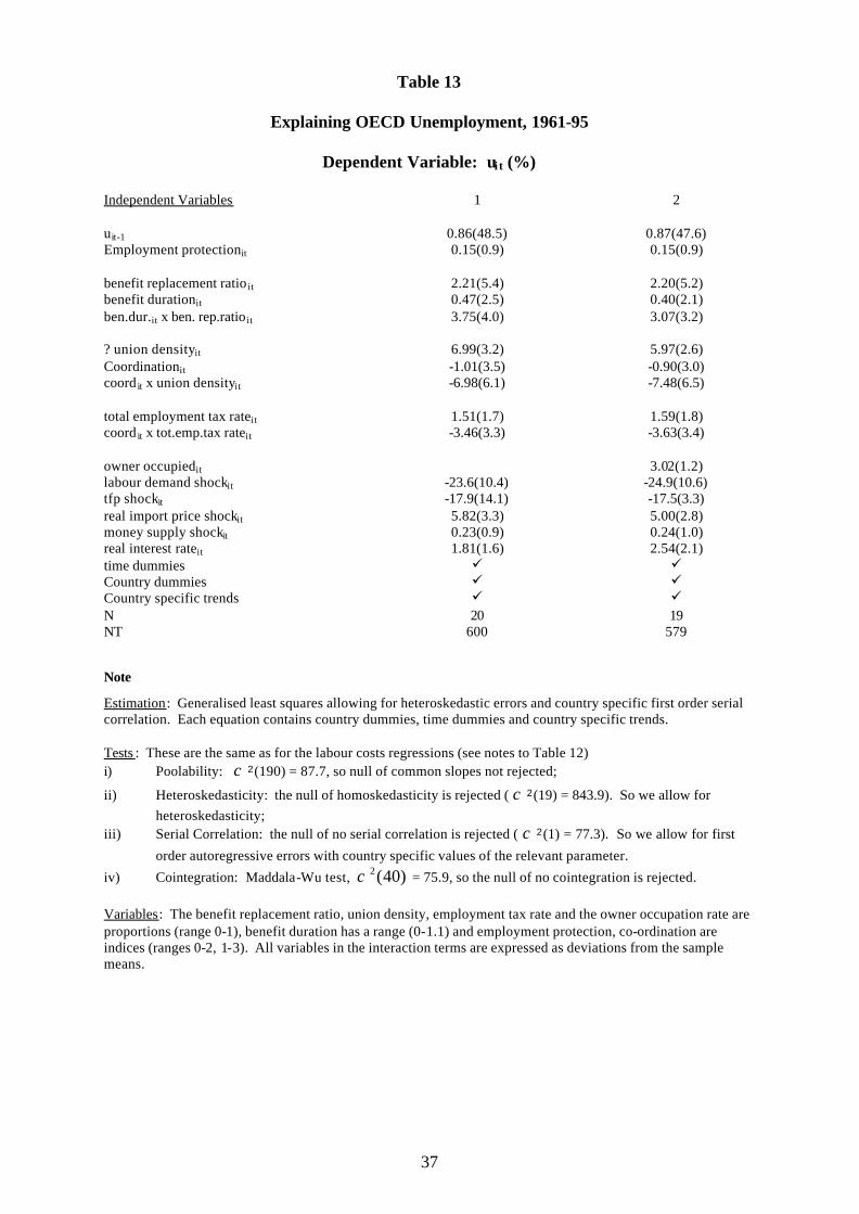
37
Table 13
Explaining OECD Unemployment, 1961-95
Dependent Variable: ui t (%) Independent Variables 1 2 uit-1 0.86(48.5) 0.87(47.6) Employment protectionit 0.15(0.9) 0.15(0.9) benefit replacement ratio it 2.21(5.4) 2.20(5.2) benefit durationit 0.47(2.5) 0.40(2.1) ben.dur.it x ben. rep.ratio it 3.75(4.0) 3.07(3.2) ? union densityit 6.99(3.2) 5.97(2.6) Coordinationit -1.01(3.5) -0.90(3.0) coord it x union densityit -6.98(6.1) -7.48(6.5) total employment tax rateit 1.51(1.7) 1.59(1.8) coord it x tot.emp.tax rateit -3.46(3.3) -3.63(3.4) owner occupiedit 3.02(1.2) labour demand shockit -23.6(10.4) -24.9(10.6) tfp shockit -17.9(14.1) -17.5(3.3) real import price shockit 5.82(3.3) 5.00(2.8) money supply shockit 0.23(0.9) 0.24(1.0) real interest rateit 1.81(1.6) 2.54(2.1) time dummies ü ü Country dummies ü ü Country specific trends ü ü N 20 19 NT 600 579
Note
Estimation: Generalised least squares allowing for heteroskedastic errors and country specific first order serial correlation. Each equation contains country dummies, time dummies and country specific trends. Tests : These are the same as for the labour costs regressions (see notes to Table 12) i) Poolability: χ 2(190) = 87.7, so null of common slopes not rejected;
ii) Heteroskedasticity: the null of homoskedasticity is rejected ( χ 2(19) = 843.9). So we allow for heteroskedasticity;
iii) Serial Correlation: the null of no serial correlation is rejected ( χ 2(1) = 77.3). So we allow for first
order autoregressive errors with country specific values of the relevant parameter.
iv) Cointegration: Maddala-Wu test, )40(2χ = 75.9, so the null of no cointegration is rejected. Variables: The benefit replacement ratio, union density, employment tax rate and the owner occupation rate are proportions (range 0-1), benefit duration has a range (0-1.1) and employment protection, co-ordination are indices (ranges 0-2, 1-3). All variables in the interaction terms are expressed as deviations from the sample means.

38
Table 14
Time Dummies, Time Trends (Units: Percentage Points)
Time Dummies
66 0.07(0.3) 76 0.69(0.6) 86 0.62(0.3)
67 0.02(0.1) 77 0.61(0.5) 87 0.79(0.4)
68 0.11(0.3) 78 0.72(0.5) 88 0.56(0.3)
69 -0.06(0.1) 79 0.59(0.4) 89 0.53(0.2)
70 0.11(0.2) 80 0.55(0.4) 90 0.98(0.4)
71 0.37(0.6) 81 1.14(0.7) 91 1.33(0.5)
72 0.50(0.7) 82 1.41(0.8) 92 1.62(0.6)
73 0.28(0.3) 83 1.21(0.7) 93 1.55(0.6)
74 0.08(0.1) 84 0.69(0.4) 94 1.14(0.4)
75 0.92(0.9) 85 0.52(0.3) 95 0.58(0.2)
Time Trends
Australia -0.054(0.5) Japan -0.059(0.6)
Austria -0.059(0.6) Netherlands -0.045(0.5)
Belgium -0.022(0.2) Norway -0.067(0.7)
Canada -0.072(0.8) NZ 0.003(0.0)
Denmark -0.078(0.8) Portugal -0.107(1.1)
Finland 0.017(0.2) Spain 0.042(0.4)
France -0.019(0.2) Sweden -0.078(0.8)
Germany (W) -0.006(0.1) Switzerland -0.041(0.4)
Ireland 0.022(0.2) UK -0.007(0.1)
Italy -0.015(0.2) US -0.026(0.3)
Note
Taken from regression reported in column 1 of Table 13. t ratios in brackets.

39
Table 15
Explaining OECD Employment/Population Ratios, 1961-95
Dependent Variable = epopi t (%)
Independent Variables 1 2 epopit-1 0.91(65.6) 0.92(66.3) Employment protectionit 0.07(0.3) 0.14(0.7) benefit replacement ratio it -2.07(4.5) -1.94(4.2) benefit durationit 0.14(0.5) 0.13(0.4) ben.dur.it x ben. rep.ratio it -4.16(4.0) -2.79(2.7) ? union densityit -11.59(4.3) -8.85(3.1) Coordinationit 1.64(7.0) 1.18(4.7) coord it x union densityit 2.72(2.2) 4.50(3.6) total employment tax rateit -2.45(2.4) -2.10(2.1) coord it x tot.emp.tax rateit 3.85(3.1) 3.86(3.1) owner occupiedit -13.34(4.7) labour demand shockit 65.18(21.3) 67.02(21.9) tfp shockit 16.80(10.5) 16.94(10.3) real import price shockit -2.22(1.2) -2.23(1.3) money supply shockit -0.14(0.3) -0.14(0.4) real interest rateit -3.65(2.7) -3.61(2.6) time dummies ü ü country dummies ü ü country specific trends ü ü N 20 20 NT 600 579
Note Estimation: Generalised least squares allowing for heteroskedastic errors and country specific first order serial correlation. Each equation contains country dummies, time dummies and country specific trends. Variables: The benefit replacement ratio, union density, employment tax rate and the owner occupation rate are proportions (range 0-1), benefit duration has a range (0-1.1), employment protection, co-ordination are indices. All variables in the interaction terms are expressed as deviations from the sample means.
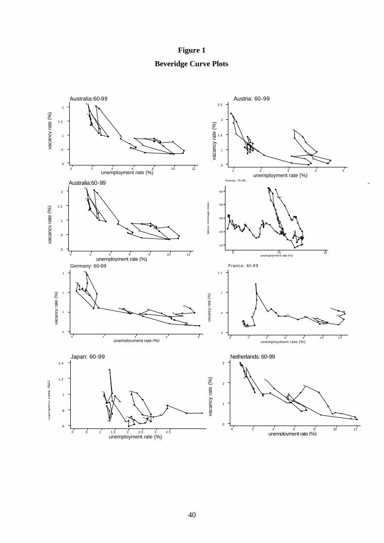
40
Figure 1
Beveridge Curve Plots
Australia:60-99
vaca
ncy
rate
(%
)
unemployment rate (%) 0 2 4 6 8 10 12
0
.5
1
1.5
2 6 0
65
70
75
80 8 5
90 95 9 9
Austria: 60-99
vaca
ncy
rate
(%)
unemployment rate (%) 1 2 3 4 5
.5
1
1.5
2
2.5
60
65 70
75 80
85
90
95 99
Australia:60-99
vaca
ncy
rate
(%)
unemployment rate (%) 0 2 4 6 8 10 12
0
.5
1
1.5
2 60
65
70
7 5
80 85
90 95 99
France: 75-99
lab
ou
r sh
ort
ag
e in
de
x
unemployment rate (%)5 10 15
10
20
30
40
50
76
77
78
79
80
81
82
83
84 858687
88
89
90
91
92
93
94
95
9697
9899
2000
-
Germany: 60-99
vaca
ncy
rate
(%
)
unemployment rate (%) 0 2 4 6 8
0
1
2
3
60
65
70
75 80
85
90 95
99
France: 60-99
vaca
ncy
rate
(%)
unemployment rate (%) 0 2 4 6 8 10 12
0
.5
1
1.5
60 6 5
70 7 5
8 0
85 9 0
95
9 9
Japan: 60-99
vaca
ncy
rate
(%
)
unemployment rate (%) 0 .5 1 1.5 2 2.5 3 3.5
.6
.8
1
1.2
1.4
6 0
65
7 0
75 8 0 85
90
95 99
Netherlands: 60-99
vaca
ncy
rate
(%
)
unemployment rate (%) 0 2 4 6 8 10 12
0
1
2
3
60
65 70
75 80
85
90
95
99

41
New Zealand: 60-96
vaca
ncy
rate
(%
)
unemployment rate (%) 0 2 4 6 8 10
0
.5
1
60 65
70
75 80
85 90 95
Norway: 60-99
vaca
ncy
rate
(%
)
unemployment rate (%) 1 2 3 4 5 6 7
.2
.4
.6
.8
60
65
70
75 80
85 90
95
99
Portugal: 74-99
vaca
ncy
rate
(%)
unemployment rate (%) 2 4 6 8 10
.1
.2
.3
.4
75
80
85
90 95
99
Spain: 77-99
vaca
ncy
rate
(%)
unemployment rate (%) 5 7.5 10 12.5 15 17.5 20 22.5 25
0
.5
1
80
85 90 95
99
Sweden: 60-99
vaca
ncy
rate
(%
)
unemployment rate (%) 0 2 4 6 8 10
0
.5
1
1.5 60 65 70
75 80
85 90
9 5 99
Switzerland: 60-99
vaca
ncy
rate
unemployment rate (%) 0 .5 1 1.5 2 2.5 3
.1
.2
.3
.4
.5
60 65 70
75
80
85
90
95
9 9
United Kingdom: 60-99
vaca
ncy
rate
(%
)
unemployment rate (%)2 4 6 8 10 12 14
.4
.6
.8
1
1.2
60 65
70 75
80 85 90 9 5
99
United States: 60-99
vacancyindex
unemployment rate (%)2 4 6 8 10
.06
.08
.1
.12
60
65 7 0
75
8085
9 09 5
9 9

42
Figure 2
A Dynamic Simulation of the Baseline Unemployment Model
Une
mpl
oym
ent
Year
Actual unemployment rate Standard dynamic simulation
Australia
1970 1975 1980 1985
2
4
6
8
10
Austria
1960 1970 1980 1990 2000
1
2
3
4
Belgium
1960 1970 1980 1990 20000
5
10
15
Canada
1960 1970 1980 1990 20000
5
10
15
Une
mpl
oym
ent
Year
Actual unemployment rate Standard dynamic simulation
Denmark
1960 1970 1980 1990 20000
5
10
Finland
1960 1970 1980 1990 20000
5
10
15
20
France
1960 1970 1980 1990 20000
5
10
15
Germany
1960 1970 1980 1990 20000
2
4
6
8
Une
mpl
oym
ent
Year
Actual unemployment rate Standard dynamic simulation
Ireland
1960 1970 1980 1990 20000
5
10
15
20
Italy
1960 1970 1980 1990 20000
5
10
Japan
1960 1970 1980 1990 2000-2
0
2
4
6
Netherlands
1960 1970 1980 1990 20000
5
10
15
Une
mpl
oym
ent
Year
Actual unemployment rate Standard dynamic simulation
Norway
1960 1970 1980 1990 20000
2
4
6
New Zealand
1975 1980 19850
2
4
6
Portugal
1975 1980 1985 1990 1995
4
6
8
10
Spain
1960 1970 1980 1990 20000
10
20
30

43
Une
mpl
oym
ent
Year
Actual unemployment rate Standard dynamic simulation
Sweden
1960 1970 1980 1990 20000
5
10
Switzerland
1960 1970 1980 1990 2000-2
0
2
4
United Kingdom
1960 1970 1980 1990 20000
5
10
15
United States
1960 1970 1980 1990 20002
4
6
8
10

44
Figure 3
A Dynamic Simulation of the Baseline Unemployment Model with the Institutions Fixed
Une
mpl
oym
ent
Year
Standard dynamic simulation All institutions fixed
Australia
1970 1975 1980 19852
4
6
8
10
Austria
1960 1970 1980 1990 2000-5
0
5
Belgium
1960 1970 1980 1990 20000
5
10
Canada
1960 1970 1980 1990 2000-5
0
5
10
Une
mpl
oym
ent
Year
Standard dynamic simulation All institutions fixed
Denmark
1960 1970 1980 1990 2000-5
0
5
10
Finland
1960 1970 1980 1990 20000
5
10
15
France
1960 1970 1980 1990 20000
5
10
15
Germany
1960 1970 1980 1990 20000
2
4
6
8
Une
mpl
oym
ent
Year
Standard dynamic simulation All institutions fixed
Ireland
1960 1970 1980 1990 20000
5
10
15
20
Italy
1960 1970 1980 1990 20000
5
10
Japan
1960 1970 1980 1990 2000-2
0
2
4
6
Netherlands
1960 1970 1980 1990 20000
5
10

45
Une
mpl
oym
ent
Year
Standard dynamic simulation All institutions fixed
Norway
1960 1970 1980 1990 2000-2
0
2
4
6
New Zealand
1975 1980 19850
2
4
Portugal
1975 1980 1985 1990 19950
5
10
Spain
1960 1970 1980 1990 20000
10
20
30
Une
mpl
oym
ent
Year
Standard dynamic simulation All institutions fixed
Sweden
1960 1970 1980 1990 2000-5
0
5
10
Switzerland
1960 1970 1980 1990 2000-2
0
2
4
United Kingdom
1960 1970 1980 1990 20000
5
10
15
United States
1960 1970 1980 1990 20004
6
8
10

46
Data Appendix
The countries in the sample are:
Australia Finland Japan Spain
Austria France Netherlands Sweden
Belgium Germany Norway Switzerland
Canada Ireland New Zealand United Kingdom
Denmark Italy Portugal United States
Where possible, the data refer to West Germany throughout.
The latest version of these data (mostly 1960-1992) may be found attached to D.P.502 at
http://cep.lse.ac.uk/papers/
Benefit Replacement Rate. Benefit entitlement before tax as a percentage of previous
earnings before tax. Data are averages over replacement rates at two earnings levels (average
and two-thirds of average earnings) and three family types (single, with dependent spouse,
with spouse at work). They refer to the first year of unemployment. Source: OECD
(Database on Unemployment Benefit Entitlements and Replacement Rates). The original
data are for every second year and have been linearly interpolated.
Benefit Duration Index. [0.6 x replacement rate in 2nd/3rd year of an unemployment spell +
0.4 x replacement rate in 4th/5th year of an unemployment spell] ÷ [replacement rate in 1st
year of an unemployment spell]. Replacement rate defined as above. Source: OECD, as
above.
Trade Union Density. This variable is constructed as the ratio of total reported union
members (less retired and unemployed members), from Ebbinghaus and Visser (2000).
Co-ordination Index (1-3). This captures the degree of consensus between the actors in
collective bargaining. 1 low, 3 high. There are two series. 1. Based on interpolations of
OECD data (OECD Employment Outlook 1994, 1997) and data made available by Michèle
Belot, described in Belot and van Ours (2000). 2. Based on data reported in OECD

47
Employment Outlook (1994), (1997), Traxler (1996), Traxler and Kittel (1999), Wallerstein
(1999), Ferner and Hyman (1998), Windmüller et al. (1987), Bamber and Lansbury (1998).
For full details, see Ochel (2000). The first series is used in all the regressions reported in the
paper.
Employment Protection Index (0-2). This captures the strictness of employment protection
laws. 0 low, 2 high. Made available by Olivier Blanchard. Based on the series used by
Lazear (1990) and that reported in OECD Employment Outlook (1999). The series is an
interpolation of 5 year averages.
Labour Taxes. This consists of the payroll tax rate plus the income tax rate plus the
consumption tax rate. These are taken from the CEP-OECD Dataset (Centre for Economic
Performance, London School of Economics) and are mainly based on OECD National
Accounts.
i) Payroll tax rate = EC/(IE-EC), EC = EPP + ESS. EPP = employers’ private pensions
and welfare plans contributions, ESS = employers’ social security contributions, IE =
compensations of employees;
ii) Income tax rate = (WC + IT)/HCR. WC = employees’ social security contributions,
IT = income taxes, HCR – households’ current receipts;
iii) Consumption tax rate = (TX – SB)/CC. TX = indirect taxes, SB = subsidies, CC =
private final consumption expenditure.
Owner Occupation Rate. Refers to the percentage of the housing stock classified as owner
occupied. The data were supplied by Andrew Oswald and have been heavily interpolated.
Not available for Portugal.
Unemployment Rate. Where possible, these correspond to OECD standardised
unemployment rates and conform to the ILO definition. For Italy; the data correspond to
“unemployment rates on US concepts” from the US Bureau of Labor Statistics. For earlier
years, we use data reported in Layard et al. (1991), Table A3. For later years we use OECD
Employment Outlook (2000), Table A and UK Employment Trends Table C 51.

48
Vacancy Rate. This is defined as the number of registered vacancies divided by employment.
The latter is total civilian employment (OECD Labour Force Statistics). The former refers to
the number of registered vacancies, to be found in OECD Main Economic Indicators. In
Canada and the United States, the vacancy data come in the form of a “help wanted”
advertising index.
Inflow Rate. This variable is the monthly inflow into unemployment divided by employment
(total civilian employment). In the UK, the data refer to the actual inflow into claimant status
(UK Employment Trends and we use the male rate because of the large variations over-time
in the benefit eligibility of unemployed women. In the remaining countries where data are
available we use the number of unemployed with duration less than one month (or 4 weeks).
Real Labour Cost per Worker. The real wage adjusted to include payroll taxes. This is
defined by the compensation of employees divided by employment and normalised on the
GDP deflator. Source: OECD, National Accounts and Main Economic Indicators.
Real Import Prices. Defined as the import price deflator normalised on the GDP deflator.
Source: OECD, National Accounts and Main Economic Indicators. The real import price
shock is the change in the log of real import prices times the share of imports in GDP (OECD
Main Economic Indicators).
Trend Productivity. Based on the Hodrick-Prescott trend of (log real GDP – log
employment).
Real Interest Rate. Long term nominal interest rate less the current rate of inflation from the
OECD Economic Outlook Database.
Total Factor Productivity (TFP). Based on the Solow residual for each country, smoothed
using a Hodrick-Prescott filter (see Nickell and Nunziata, 2000, for more detail). There are
two versions of the TFP shock. 1. Three year moving average of ? 2 (so low residual). This
is used in the labour cost equations in Table 12. 2. The cyclical component of TFP, i.e. the
deviation of the Solow residual from its HP filter trend. This is used in the unemployment
and employment equations (Tables 13, 15).

49
Labour Demand Shock. Residuals from country specific employment equations, each being a
regression of employment on lags of employment and real wages.
Money Supply Shock. ? 2 ln (money supply) from OECD Economic Outlook database.
Employment Population Ratio. Total civilian employment normalised on the working age
population (15-64), from CEP OECD dataset, updated.

50
References
Abbring, J. H., Van Den Berg, G. J and Van Our, J. C. (1999), ‘The Effect of Unemployment Insurance Sanctions on the Transition Rate from Unemployment to Employment’, Tinbergen Institute, University of Amsterdam.
Addison, J. T. and Grosso, J-L. (1996), ‘Job Security Provisions and Unemployment:
Revised Estimates’, Industrial Relations 35, pp.585-603. Baltagi, B. (1995), Econometric Analysis of Panel Data, John Wiley and Sons. Bamber, G. J. and R. D. Lansbury (eds.), (1998), International and Comparative Employment
Relations. A Study of Industrialised Market Economies (London. Thousand Oaks, New Delhi)
Belot, M. and van Ours, J. C. (2000), ‘Does the Recent Success of Some OECD Countries in
Lowering their Unemployment Rates Lie in the Clever Design of their Labour Market Reforms?’, IZA Discussion Paper No. 147, April, Bonn, Germany.
Bentolila, S. and Bertola, G. (1990), ‘Firing Costs and Labour Demand: How Bad is Euro
Sclerosis?’, Review of Economic Studies, 57, pp.381-402. Blanchard, O. and Katz, L. (1999), ‘What We Know and Do Not Know about the Natural
Rate of Unemployment’, Journal of Economic Perspectives. Blanchard, O. and Wolfers, J. (2000), ‘The Role of Shocks and Institutions in the Rise of
European Unemployment: The Aggregate Evidence’, The Economic Journal, (Conference Papers), 110, pp.C1-C33.
Booth, A., Burda, M., Calmfors, L., Checchi, D., Naylor, R., Visser, J. (2000), ‘What do
Unions do in Europe?’, A Report for the Fondazione Rodolfo DeBenedetti, Milan. Bover, O., Garcia-Perea, P., Portugal, P, (1998), ‘A Comparative Study of the Portuguese and
Spanish Labour Markets’, Banco de Espana, mimeo. Carling, K., Edin, P-A., Herkman, A. and Holmlund, B. (1996), ‘Unemployment Duration,
Unemployment Benefits and Labor Market Programs in Sweden’, Journal of Public Economics, 59, pp.313-334.
Carling, K., Holmlund, B. and Vejsiu, A. (1999), ‘Do Benefit Cuts Boost Job Findings?
Swedish Evidence from the 1990s’, Swedish Office of Labour Market Policy Evaluation, Working Paper 1999: 8, Uppsala: Sweden.
Coe, D. T. and Snower, D. J. (1997), ‘Policy Complementarities: The Case for Fundamental
Labour Market Reform’, CEPR Discussion Paper No. 1585, CEPR: London. Cully, M. and S. Woodland, ‘Trade Union Membership and Resulting Labour Market
Trends’, Labour Market Trends, Office of National Statistics, July.

51
Daniel, W. W. and Stilgoe, E. (1978), The Impact of Employment Protection Laws, Policy Studies Institute: London.
Danish Ministry of Finance (1999), The Danish Economy: Medium Term Economic Survey,
Ministry of Finance: Copenhagen. Daveri, F. and Tabellini, G. (2000), ‘Unemployment, Growth and Taxation in Industrial
Countries’, Economic Policy (April), pp.49-90. Disney, R. (2000), ‘Fiscal Policy and Employment 1: A Survey of Macroeconomic Models,
Methods and Findings’, IMF, mimeo. Ebbinghaus, B. and Visser, J. (2000), Trade Unions in Western Europe, MacMillan: London. Elmeskov, J., Martin, J. P. and Scarpetta, S. (1998), ‘Key Lessons for Labour Market
Reforms: Evidence from OECD Countries’ Experiences’, Swedish Economic Policy Review, 5(2), pp.205-252.
Ferner, A. and Hyman, R. (eds), (1998), Changing Industrial Relations in Europe, 2nd edition
Malden: Oxford. Fitoussi, J-P., Jestaz, D., Phelps, E. S., Zoega, G. (2000), ‘Roots of the Recent Recoveries:
Labor Reforms or Private Sector Forces?’, Brookings Papers on Economic Activity, 1, pp.237-291.
Gregg, P., Machin, S. and Manning, A. (2000), ‘Mobility and Joblessness’, London School of
Economics, Centre for Economic Performance, mimeo. Ham, J. and Rea, S. (1987), ‘Unemployment Insurance and Male Unemployment Duration in
Canada’, Journal of Labor Economics, 5, pp.325-353. Harkman, A. (1997), ‘Unemployment Compensation and Unemployment Duration – What
was the Effect of the Cut in the Replacement Rate from 90 to 80 Percent?’ in A. F. Harkman; K. Jansson; K. Kallberg and L. Öhrn (eds.), Unemployment Insurance and the Functioning of the Labour Market, The Swedish National Labour Market Board: Stockholm.
Holmlund, B. (1998), ‘Unemployment Insurance in Theory and Practice’, The Scandinavian
Journal of Economics, 100(1), pp.113-141. Hoon, H. T. and Phelps, E. S. (1992), ‘Macroeconomic Shocks in a Dynamized Model of the
Natural Rate of Unemployment’, American Economic Review, 82. Hunt, J. (1995), ‘The Effect of Unemployment Compensation on Unemployment Duration in
Germany’, Journal of Labor Economics, 13, pp.88-120. Katz, L. F. (1998), ‘Wage Subsidies for the Disadvantaged’ in R. Freeman and P. Gottschalk
(eds.), Generating Jobs, Russell Sage Foundation: New York.

52
Katz, L. and Meyer, B. (1990), ‘The Impact of Potential Duration of Unemployment Benefits on the Duration of Unemployment’, Journal of Public Economics, 41, pp.45-72.
Layard, R., Nickell, S. J. and Jackman, R. (1991), Unemployment: Macroeconomic
Performance and the Labour Market, Oxford University Press: Oxford. Lazear, E. P. (1990), ‘Job Security Provisions and Employment’, Quarterly Journal of
Economics, 105, pp.699-726. Maddala, G. S. and Wu, S. (1996), ‘A Comparative Study of Unit Root Tests with Panel Data
and a New Simple Test: Evidence from Simulations and the Bootstrap’, Ohio State University, mimeo.
Martin, J. (2000), ‘What Works among Active Labour Market Policies? Evidence from
OECD Countries’, OECD Economic Studies, No.30, pp.79-112, OECD: Paris. Meyer, B. (1995), ‘Lessons from the US Unemployment Insurance Experiments’, Journal of
Economic Literature, 33, pp.91-131. Millward, N., Smart, D. and Hawes, W. (1992), Workplace Industrial Relations in Transition,
Aldershot. Milner, S. (1995), ‘The Coverage of Collective Pay-setting Institutions in Britain, 1895-
1990’, British Journal of Industrial Relations, 33(1), pp.71-91. Mortensen, D.T. and Pissarides, C.A. (1994), ‘Job Creation and Job Destruction in the
Theory of Unemployment’, Review of Economic Studies, 61, pp.397-415. Mortensen, D. T. and Pissarides, C. A. (1999), ‘New Developments in Models of Search in
the Labor Market’ in Ashenfelter, O. and Card, D. (eds.), Handbook of Labor Market, North Holland: Amsterdam.
Nickell, S. J. (1990), ‘Unemployment: A Survey’, Economic Journal. Nickell, S. J. and Layard, R. (1999), ‘Labour Market Institutions and Economic Performance’
in O.Ashenfelter and D. Card (eds.), Handbook of Labor Economics, Vol. 3, North Holland: Amsterdam.
Nickell, S. J. (1997), ‘Unemployment and Labour Market Rigidities: Europe versus North
America’, Journal of Economic Perspectives, 11(3), pp.55-74. Nickell, S. J. and Nunziata, L. (2000), ‘Employment Patterns in OECD Countries’ Centre for
Economic Performance Discussion Paper No. 448, London School of Economics. Ochel, W. (2000), ‘Collective Bargaining Coverage’, Ifo Institute for Economic Research,
Munich. Ochel, W. (2000), ‘Collective Bargaining (Centralization and Co-ordination)’, Ifo Institute
for Economic Research: Munich.

53
OECD (1990), Employment Outlook, OECD: Paris. OECD (2000), Employment Outlook, OECD: Paris. OECD (1997), Employment Outlook, OECD: Paris. OECD (1994), The OECD Jobs Study, Evidence and Explanations, Vols. I and II, OECD:
Paris. Oswald, A. (1997), ‘The Missing Piece of the Unemployment Puzzle’, Inaugural Lecture,
University of Warwick, November. Phelps, E. S. (1994), Structural Slumps, The Modern Equilibrium Theory of Unemployment,
Interest and Assets, Harvard University Press: Cambridge MA. Pissarides, C. (1998), ‘The Impact of Employment Tax Cuts on Unemployment and Wages;
the Role of Unemployment Benefits and Tax Structure’, European Economic Review, 47, pp.155-183.
Pissarides, C. A., (1990), Equilibrium Unemployment Theory, Basil Blackwell: Oxford. Roy, S. (1957), Some Aspects of Multivariate Analysis, John Wiley and Sons. Scarpetta, S. (1996), ‘Assessing the Role of Labour Market Policies and Institutional Settings
on Unemployment: A Cross Country Study’, OECD Economic Studies, 26: pp.43-98. Solow, R. (2000), ‘Unemployment in the United States and in Europe: A Contrast and the
Reasons’, CES ifo Forum, Spring. Soskice, D. (1991), ‘Wage Determination: The Changing Role of Institutions in Advanced
Industrialised Countries’, Oxford Review of Economic Policy, 6, pp.36-61. Traxler, F. (1996), ‘Collective Bargaining and Industrial Change: A Case of
Disorganization? A Comparative Analysis of Eighteen OECD Countries’, European Sociological Review, Vol.12, No.3, pp.271-287.
Traxler, F. and Kittel, B. (1999), ‘The Bargaining System and Performance: A Comparison
of 18 OECD Countries’, Comparative Political Studies, (forthcoming). Van Den Berg, G., Van Der Klaauw, B. and Van Ours, J. C. (1999), ‘Punitive Sanctions and
the Transition Rate from Welfare to Work’, Tinbergen Institute, University of Amsterdam.
Visser, J. (1996), ‘Unionisation Trends. The OECD Countries Union Membership File’,
Centre for Research of European Societies and Labour Relations, University of Amsterdam.
Wallerstein, M. (1999), ‘Wage-Setting Institutions and Pay Inequality in Advanced Industrial
Societies’, American Journal of Political Science, 43(3), July.

54
Windmiller, J.P. (1987), Collective Bargaining in Market Economics: A Reappraisal, (Geneva: ILO).
Zellner, A. (1962), ‘A Efficient Method of Estimating Seemingly Unrelated Regression and
Tests for Aggregation Bias’, Journal of the American Statistical Association, 57.

CENTRE FOR ECONOMIC PERFORMANCE Recent Discussion Papers
501 S. Redding M. Vera-Martin
Factor Endowments and Production in European Regions
500 Edited by D. Marsden and H. Stephenson
Labour Law and Social Insurance in the New Economy: A Debate on the Supiot Report
499 A. Manning A Generalised Model of Monopsony
498 A. Charlwood Why Do Non-Union Employees Want to Unionise? Evidence from Britain
497 M. Keil D. Robertson J. Symons
Minimum Wages and Employment
496 A. Di Liberto J. Symons
Education and Italian Regional Development
495 S. Redding A. J. Venables
Economic Geography and International Inequality
494 A. Bryson Union Effects on Managerial and Employee Perceptions of Employee Relations in Britain
493 D. Metcalf British Unions: Dissolution or Resurgence Revisited
492 R. Gomez S. M. Lipset N. Meltz
Frustrated Demand for Unionisation: the Case of the United States and Canada Revisited
491 S. Burgess J. Lane D. Stevens
Jobs, Workers and Changes in Earnings Dispersion
490 S. Burgess S. Profit
Externalities in the Matching of Workers and Firms in Britain
489 S. Nickell G. Quintini
Nominal Wage Rigidity and the Rate of Inflation
488 S. Nickell J. Van Reenen
Technological Innovation and Performance in the United Kingdom

487 M. M. Tudela Explaining Currency Crises: A Duration Model Approach
486 D. Sturm Product Standards, Trade Disputes and Protectionism
485 G. Duranton V. Monastiriotis
Mind the Gaps: The Evolution of Regional Inequalities in the UK 1982-1997
484 H. G. Overman Y. Ioannides
Zipfs Law for Cities: An Empirical Examination
483 H. G. Overman Y. Ioannides
Cross Sectional Evolution of the US City Size Distribution
482 Y. Ioannides H. G. Overman
Spatial Evolution of the US Urban System
481 H. G. Overman Neighbourhood Effects in Small Neighbourhoods
480 S. Gomulka Pension Problems and Reforms in the Czech Republic, Hungary, Poland and Romania
479 S. Nickell T. Jones G. Quintini
A Picture of the Job Insecurity Facing British Men
478 C. Dougherty Numeracy, Literacy and Earnings: Evidence from the National Longitudinal Survey of Youth
477 P. Willman The Viability of Trade Union Organisation: A Bargaining Unit Analysis
476 D. Marsden S. French K. Kubo
Why Does Performance Pay De-Motivate? Financial Incentives versus Performance Appraisal
475 S. Gomulka Macroeconomic Policies and Achievements in Transition Economies, 1989-1999
474 S. Burgess H. Turon
Unemployment Dynamics, Duration and Equilibrium: Evidence from Britain
473 D. Robertson J. Symons
Factor Residuals in SUR Regressions: Estimating Panels Allowing for Cross Sectional Correlation
To order a discussion paper, please contact the Publications Unit Tel 020 7955 7673 Fax 020 7955 7595 Email [email protected]
Web site http://cep.lse.ac.uk