The Asymptotic Size and Power of the Augmented

Dickey-Fuller Test for a Unit Root

Efstathios Paparoditis∗ Dimitris N. Politis†

Abstract

It is shown that the limiting distribution of the augmented Dickey-Fuller

(ADF) test under the null hypothesis of a unit root is valid under a very general

set of assumptions that goes far beyond the linear AR(∞) process assumption

typically imposed. In essence, all that is required is that the error process driving

the random walk possesses a continuous spectral density that is strictly positive.

Furthermore, under the same weak assumptions, the limiting distribution of the

ADF test is derived under the alternative of stationarity, and a theoretical ex-

planation is given for the well-known empirical fact that the test’s power is a

decreasing function of the chosen autoregressive order p. The intuitive reason for

the reduced power of the ADF test is that, as p tends to infinity, the p regressors

become asymptotically collinear.

Key words: Autoregressive Representation, Hypothesis Testing, Random Walk.

Acknowledgment. The authors are grateful to Essie Maasoumi, Peter Phillips,

David Stoffer and Adrian Trapletti for helpful suggestions, and to Nan Zou for

computational support. Many thanks are also due to Li Pan and to the students

of the MATH181E class at UCSD in Fall 2012 for their valuable input on the

real data example of Section 3. The research of the second author was partially

supported by NSF grants DMS 12-23137 and DMS 13-08319.

∗Dept. of Mathematics and Statistics, University of Cyprus, P.O.Box 20537, CY 1678 Nicosia,

CYPRUS; stathisp@ucy.ac.cy†Department of Mathematics, University of California—San Diego, La Jolla, CA 92093-0112, USA;

dpolitis@ucsd.edu

1

1 Introduction

Testing for the presence of a unit root is a widely investigated problem in econometrics;

cf. Hamilton (1994) or Patterson (2011) for extensive treatments of this topic. Given a

stretch of time series observations X1, X2, . . . , Xn, one of the commonly used tests for

the null hypothesis of a unit root, is the so-called augmented Dickey-Fuller (ADF) test.

This test decides about the presence of a unit root in the data generating mechanism

by using the ordinary least squares (OLS) estimator ρn of ρ, obtained by fitting the

regression equation

Xt = ρXt−1 +p∑

j=1

aj,p∆Xt−j + et,p, (1.1)

to the observed stretch of data. In the above notation, ∆Xt = Xt − Xt−1, while the

order p is allowed to depend on n, i.e., p is short-hand for pn, in a way that is related

to the assumptions imposed on the underlying process. In particular, under the null

hypothesis H0 : ρ = 1, it is commonly assumed that Xt is obtained by integrating a

linear, infinite order autoregressive process, (AR(∞)), i.e., that

Xt = Xt−1 + Ut, t = 1, 2, . . . , (1.2)

where X0 = 0 and

Ut =∞∑

j=1

ajUt−j + et. (1.3)

Here {et} is a sequence of independent, identically distributed (i.i.d.) random variables

having mean zero and variance 0 < σ2e < ∞. Stationarity and causality of {Ut} is

ensured by assuming that∑∞

j=1 |j|s|aj| < ∞ for some s ≥ 1 and∑∞

j=1 ajzj 6= 0 for all

|z| ≤ 1.

To test H0, Dickey and Fuller (1979) proposed the studentized statistic

tn =ρn − 1

Std(ρn), (1.4)

where Std(ρn) denotes an estimator of the standard deviation of the OLS estimator ρn.

The asymptotic distribution of tn under H0 is non-standard and is well known in the

2

literature. Dickey and Fuller (1979) and Dickey and Fuller (1981) derived this distri-

bution under the assumption that the order of the underlying autoregressive process is

finite and known. Said and Dickey (1984) extended this result for the case where the

innovation process {Ut} driving the random walk (1.2) is an invertible autoregressive

moving-average (ARMA) process, i.e., an AR(∞) process with exponentially decaying

coefficients. Ng and Perron (1995) relaxed the assumptions needed on the rate at which

the order p in (1.1) increases to infinity with n. Chang and Park (2002) established

the same limiting distribution of tn by further relaxing the assumptions regarding the

rate at which p increases to infinity, by allowing for a polynomial decrease of the coef-

ficients aj in the AR(∞) representation (1.3) and by assuming a martingale difference

structure instead of i.i.d. innovations et, that is, by assuming that E(et|Et−1) = 0 and

n−1 ∑nt=1 E(e2

t |Et−1) → σ2, as n → ∞, where El = σ({et : t ≤ l}) is the σ-algebra

generated by the random variables {el, el−1, . . .}.To derive the power behavior of the test under the alternative hypothesis H1 : ρ < 1,

the limiting distribution of tn is required under the assumption that {Xt} is a stationary

process. Investigating the power of the ADF-test for fixed (stationary) alternatives,

has attracted less interest in the literature. Nabeya and Tanaka (1990) and Perron

(1991) analyzed the limiting power of unit root tests for sequences of local alternatives.

For a first order autoregression, Abadir (1993) gives closed forms for the distribution of

certain statistics leading to the derivation of the limiting distribution of unit root tests

under the null and the alternative. For the ADF unit root test, Lopez (1997) considered

the asymptotic distribution of ρn under the alternative that {Xt} is a causal and

invertible ARMA process; nevertheless, apart from the restrictive ARMA set-up, there

is a flaw in his derivations. To elaborate, Lopez (1997) replaces the regression equation

(1.1) by a regression that contains only levels of the Xt’s; but this replacement is not

justified when p is of larger order of magnitude than n1/8 as our Remark 2.4 explains.

Testing for the presence of a unit root remains an active area of econometric re-

search. As regards the ADF test, Elliot et al. (1996) proposed nearly efficient tests

3

while Harvey et al. (1999) discussed issues caused by the uncertainty about the deter-

ministic trend and the initial values. The effects of the initial value in unit root testing

were definitively investigated in the influential paper by Muller and Elliot (2003). In ad-

dition, Muller (2005, 2007) considered strongly autocorrelated time series and studied

size and power properties of unit root tests in a local-to-unity asymptotic framework.

Notably, under unit root (or local-to-unity) assumptions, the initial value will have

an effect on the asymptotic distribution of the test statistic only if it is of order of

magnitude of at least√

n. However, in the standard asymptotic framework (that we

also adopt), the effect of a fixed initial value vanishes as n → ∞.

A different and interesting direction of research in unit root testing is described by

so-called ‘tuning parameters free’ tests. Such tests have been considered by Breitung

(2002), Muller and Watson (2008) and Nielsen (2009). By means of an appropriate

rescaling, these tests bypass the problem of estimating the long-run variance which

appears as a nuisance parameter in unit root testing. In the context of the well-known

Phillips and Perron test—see Phillips (1987) and Phillips and Perron (1988)—, this

nuisance parameter is estimated via non-parametric spectral methods whereas, in the

context of the ADF test, the same problem is addressed via augmenting the regression

equation by p lagged differences, and allowing for p to increase with sample size. Finally,

recall that the popular KPSS stationarity test of Kwiatkowski et al. (1992) can also

be employed for unit root testing; see e.g. Shin and Schmidt (1992).

Despite these developments, our paper contributes towards a deeper understanding

of the ADF test. Firstly, we show that the asymptotic distribution of the ADF test

statistic under the null hypothesis of a unit root is valid under a most general set

of assumptions regarding the innovation process {Ut} driving the random walk (1.2).

These assumptions go far beyond the AR(∞) linear process class (1.3). In particular,

we prove validity of the limiting distribution of tn under the general condition that

the stationary process {Ut} possesses a Wold-type, AR-representation with respect to

white noise errors εt; see eq. (2.6) in what follows. This much wider class of stationary

4

processes should not be confused with the linear AR(∞) class (1.3) driven by i.i.d. or

by martingale difference innovations. In fact, the class of processes admitting a Wold-

type, AR-representation with respect to white noise errors consists of all zero mean,

second order stationary (linear or nonlinear) processes having a continuous and strictly

positive spectral density; cf. Pourahmadi (2001) for details.

Secondly, under the same set of general assumptions on the underlying stationary

process {Ut}, we establish the limiting distribution of the ADF-test tn under the alter-

native hypothesis in which {Xt} is stationary. It turns out that under the alternative,

the estimator ρn is only√

n/p—consistent, and therefore, its convergence rate is con-

siderably smaller compared to the n–consistency of the same estimator under the null,

and to the√

n convergence rate of other test statistics under the alternative as, e.g.,

the test of Philips and Perron (1988). We make the case that the underlying reason

for the slow rate of convergence of ρn under the alternative is that the regressors in

equation (1.1) become asymptotically collinear as p diverges; this is a surprising and

novel result in the literature of unit root tests. We analyze this phenomenon, and show

that this collinearity problem is responsible for the reduced power of the ADF-test,

and gives a theoretic basis for the empirically observed fact that the power of the ADF

test is a decreasing function of the order p—see e.g. Figure 9.5 of Patterson (2011).

The remainder of the paper is organized as follows. Section 2 states the main

assumptions imposed on the underlying process {Ut} and derives the asymptotic dis-

tribution of the ADF test tn under the null hypothesis of a unit root. The asymptotic

behavior of tn under the alternative of stationarity is also derived in Section 2, and its

consequences for the power properties of the ADF test are discussed. Section 3 show

cases a real data example where the reduced power of the ADF test is manifested in an

extreme fashion, and underscores the importance of properly choosing the order p in

practice. Section 4 presents the results of a simulation experiment that gives empirical

confirmation of some of the theoretical results derived in Section 2. All technical proofs

are deferred to Section 5.

5

2 Asymptotic Properties of the ADF test

2.1 Assumptions

We first state the conditions we impose on the dependence structure of the underlying

second order stationary process {Ut} that drives the random walk under the null. As-

suming that {Ut} is purely non-deterministic, i.e., that it possesses as spectral density

whose logarithm is integrable, then the Wold representation yields

Ut =∞∑

j=1

αjεt−j + εt (2.5)

where∑∞

j=1 α2j < ∞ and εt is a zero mean, uncorrelated process with 0 < V ar(εt) =

σ2ε < ∞. We slightly restrict the above class of stationary processes to the one satisfying

the following assumption.

Assumption 1

(i) The autocovariance function γU (h) = Cov(Ut, Ut+h), h ∈ ZZ, of U = {Ut, t ∈ ZZ}satisfies

∑h∈ZZ |γU(h)| < ∞, and the spectral density fU of U is strictly positive,

i.e., fU (λ) > 0 for all λ.

(ii) E(ε4t ) < ∞ and the process {εt} satisfies the following weak dependence condi-

tion:∑∞

n=1 n‖P1(εn)‖ < ∞, where Pt(Y ) = E(Y |Ft)−E(Y |Ft−1) and Fs = (. . . , εs−1, εs).

Here, and in the rest of the paper, the norm ‖ · ‖ is taken to be the Lp norm with

p = 4.

The Wold representation (2.5) is an MA(∞) equation for Ut with respect to its in-

novations εt. Assumption 1(i) allows for an alternative representation of Ut with re-

spect to the same white noise given in (2.5). In fact, because of the summability

of the autocovariance function, the process {Ut} has a continuous spectral density

fU (λ) = (2π)−1 ∑h∈ZZ γU(h) cos(λh). This together with the strict positivity of fU(λ)

6

implies that {Ut} possesses a so-called Wold-type AR-representation, that is, Ut can be

expressed as

Ut =∞∑

j=1

bjUt−j + εt, (2.6)

where εt is the same white noise innovation process as the one appearing in the Wold

representation (2.5). Furthermore, the coefficients bj are absolutely summable, i.e.,∑∞

j=1 |bj| < ∞ and b(z) = 1 − ∑∞k=1 bjz

j 6= 0 for |z| ≤ 1; see Pourahmadi (2001),

Lemma 6.4.

The Wold-type AR-representation (2.6) of Ut with respect to the white noise process

εt should not be confused with the rather strong assumption of a linear AR(∞) process

with respect to i.i.d. innovations. For example, one important difference between the

class of process obeying a Wold-type AR-representation and the class of linear AR(∞)

processes (1.3) is the linearity of the optimal predictor. In fact, for processes in the class

(1.3) with i.i.d. or with martingale difference errors, the optimal k-step ahead predictor,

is always the linear predictor. That is, for positive k, the general L2-optimal predictor

of Ut+k based on its past Ut, i.e., the conditional expectation E(Ut+k|Us, s ≤ t), is for

processes (1.3) with i.i.d. or with martingale difference innovations, identical to the

best linear predictor PMt(Ut+k). Here PC(Y ) denotes orthogonal projection of Y onto

the set C and Mt = span{Uj : j ≤ s}, i.e., the closed linear span generated by the

random variables {Uj : j ≤ s}. This linearity property of the L2-optical predictor is

not shared by processes that only admit a Wold-type AR-representation with respect

to white noise innovations.

It is apparent that the class of processes having a Wold-type AR-representation is

very large, and includes basically all time series, linear or nonlinear, as long as they

possess a strictly positive and continuous spectral density. The difference between the

Wold-type AR-representation and the linear AR(∞) property (1.3) is further illustrated

7

by means of the following two examples.

Example 1: (Non causal linear processes) Consider the process Ut = φUt−1 + et,

with |φ| > 1, and et a zero mean i.i.d. process with variance σ2e . Notice that {Ut} is

stationary but it does not belong to the linear AR(∞) class (1.3) since it is not causal

(the root of 1 − φz = 0 lies outside the unit disc). However, for εt = φ−2(et − (φ2 −1)

∑j≥1 φ−jet+j), Ut has the AR-representation Ut = bUt−1 + εt with b = 1/φ and the

(causal) Wold representation Ut =∑∞

j=1 bjεt−j with respect to the white noise process

{εt}, where E(εt) = 0 and V ar(εt) = φ−2σ2e .

Example 2: (Non invertible linear processes) Consider the process Ut = θet−1+et,

with |θ| > 1, and et a zero mean i.i.d. process with variance σ2e . Notice that {Ut}

is stationary but it does not belong to the linear AR(∞) class (1.3) since it is not

invertible (the root of 1 − θz = 0 lies outside the unit disc). Now, for εt = et + (θ−1 −θ)

∑∞j=1 θ−j+1et−j we get Ut = εt − θ−1εt−1 and therefore, Ut has the AR-representation

Ut =∑∞

j=1 bUt−j + εt, bj = −(1/θ)j , with respect to the white noise process {εt}. Here

E(εt) = 0 and V ar(εt) = σ2e(1 + θ2 − θ4).

Assumption 1(ii) is imposed in order to control the dependence structure of the

innovation process {εt} and consequently of Ut; cf. Wu and Min (2005). It is based

on the concept of weak dependence introduced by Wu (2005) and allows together with

(2.5) for a very broad class of possible processes. Wu and Min (2005) give many

examples of processes belonging to this class, including many well-known nonlinear

processes, e.g., ARCH/GARCH processes, threshold autoregressive processes, bilinear

processes and random coefficient autoregressions.

Note that instead of the weak dependence assumption above, other measures could

be also used to control the dependence structure of the innovations process {εt} as

well. For instance, the results presented in this paper can be derived also under the

alternative assumption that the innovation process {εt} in (2.5) is strong mixing with

strong mixing coefficient αm satisfying∑∞

m=1 α1/2m < ∞. In any case, Assumption 1(ii)

8

extends considerably the class of stationary process allowed and goes far beyond the

limited class of linear autoregressive processes with i.i.d. innovations or innovations

that form martingale differences.

Based on Assumption 1 regarding the class of stationary process {Ut}, Assumption

2 below specifies the generation mechanism of the underlying and observable process

X = {Xt, t ≥ 0}.

Assumption 2 The process X satisfies one (and only one) of the following two

conditions:

(i) (Unit root case:) X0 = 0 and Xt = Xt−1 + Ut for t = 1, 2, . . ..

(ii) (Stationary case:) Xt = Ut, for t = 0, 1, 2, . . .,

where {Ut} is the second order stationary process specified in Assumption 1.

The assumption X0 = 0 simplifies notation and does not affect the asymptotic

results of this paper for the unit root case. It can be replaced by other assumptions

concerning the starting value X0 provided this random variable remains bounded in

probability. Assumption 2 simply states that Xt is either a stationary process satisfying

Assumption 1 or it is obtained by integrating such a stationary process.

Notice that if Assumption 2 is true, then Xt obeys also the useful representation

Xt = ρXt−1 +∞∑

j=1

aj∆Xt−j + εt, (2.7)

with εt the white noise process discussed in Assumption 1. To see this, notice that

(2.7) is obviously true if Assumption 2(i) is satisfied with the choices ρ = 1 and

∆Xt−1 = Xt − Xt−1 = Ut. Furthermore, if Assumption 2(ii) is true then it is easily

verified that Xt = (∑∞

j=1 bj)Xt−1 −∑∞

j=1(∑∞

s=j+1 bs)∆Xt−j + εt, which implies that also

in this case (2.7) is true with

ρ =∞∑

j=1

bj, and aj = −∞∑

s=j+1

bs, j = 1, 2, . . . .

9

Now, let

ρmin = inf{ρ =

∞∑

j=1

bj : bj, j = 1, 2, . . . and b(z) = 1 −∞∑

j=1

bjzj 6= 0 for |z| ≤ 1

}.

The null and alternative hypothesis of interest can then be stated as

H0 : ρ = 1, H1 : ρ ∈ (ρmin, 1). (2.8)

Notice that H0 is equivalent to Assumption 2(i) while H1 to Assumption 2(ii). The

range of values of ρ under the alternative H1 is an interval since B = {bj, j = 1, 2, . . . :

b(z) 6= 0 for |z| ≤ 1} is a convex set and the mapping g : B → IR with g(b1, b2, . . .) =∑∞

j=1 bj ≡ ρ is continuous. Notice that ρmin < −1 is also possible, for instance if

Ut = εt − θεt−1 with θ ∈ (0.5, 1).

Remark 2.1 It is common in the econometric literature to state Assumption 2 in the

following different form:

Xt = aXt−1 + Ut, (2.9)

where {Ut} is some zero mean, second order stationary process satisfying certain condi-

tions. In this formulation, the case a = 1 is associated with the null hypothesis of unit

root, while the case |a| < 1 with the alternative; see among others Ng and Perron (1995)

and Chang and Park (2002). It is easily seen that the above formulation is a restate-

ment of Assumption 2 in the sense that in both cases the same conditions are imposed

on the underlying process {Xt}. If a = 1 this is obviously true while for |a| < 1, using

the backshift operator LsXt = Xt−s we have that Xt = (1 − aL)−1Ut =∑∞

j=0 ajUt−j

and {Xt} is stationary. However, if (2.9) is considered as a model for Xt, then iden-

tifiability and interpretability problems occur for the parameter a unless, of course,

a = 1. To see why, let Xt be a stationary series, and define the new stationary series

Vt = Xt − bXt−1 where b is arbitrary; i.e., in the stationary case, eq. (2.9) holds true

for any value of the parameter a as long as it is not one. To make the parameter a

identifiable in the stationary case, an additional condition must be imposed, e.g., that

the series Ut is the innovation series of Xt. Our Assumption 2 avoids these difficulties.

10

2.2 Limiting Distribution under the Null

The following theorem establishes the limiting distribution of the test statistic tn under

H0 in (2.8). It shows that this limiting distribution is identical to that obtained under

the AR(∞) linearity or weak linearity assumption for {Ut}; cf. Dickey and Fuller

(1981) and Chang and Park (2002).

Theorem 2.1 Let Assumption 1 and Assumption 2(i) be satisfied and suppose that

pn → ∞ as n → ∞ such that pn/√

n → 0. Then

tn ⇒∫ 1

0W (t)dW (t)

/( ∫ 1

0W 2(t)dt

)1/2,

where {W (t), t ∈ [0, 1]} is the standard Wiener process on [0, 1].

By the above theorem, an asymptotic α-level test of the null hypothesis of a unit

root is given by rejecting H0 whenever tn is smaller than Cα, where Cα is the lower α-

percentage point of the distribution of∫ 10 W (t)dW (t)

/√∫ 10 W 2(t)dt. Notice that since

the class of stationary processes satisfying Assumption 1 is very rich and contains as

special case many linear and nonlinear processes including the commonly used linear

AR(∞) process driven by i.i.d. innovations or by martingale differences, Theorem 2.1

generalizes considerably previous results regarding the limiting distribution of the ADF-

test under the null hypothesis of a unit root.

Remark 2.2 Theorem 2.1 can be also extended to cover the case of a deterministic

trend. In particular, if the process under H0 is generated by the equation Yt = Xt+a+bt

, where (Xt) satisfies Assumption 2(i) and the regression equation

Yt = ρYt−1 + a + bt +p∑

j=1

aj,p∆Xt−j + et,p,

is fitted to the observed time series Y1, Y2, . . . , Yn, then the distribution of the least

squares estimator ρn of ρ is the same as the one given in Thorem 2.1 with the standard

11

Brownian motion W (t) replaced by

W (t) = W (t) + (6t − 4)∫ 1

0W (s)ds − (12t − 6)

∫ 1

0sW (s)ds.

2.3 Behavior Under the Alternative

Before studying the large-sample distribution of the least squares estimator ρn un-

der the alternative of stationarity, we discuss an asymptotic collinearity problem that

occurs when regression equation (1.1) is fitted to a time series stemming from a sta-

tionary process. This collinearity problem is essential for understanding the effects of

choosing the truncation parameter p on the power behavior of the test. The following

proposition summarizes this behavior, and is of interest in its own right.

Proposition 2.1 Let {Wt, t ∈ ZZ} be a zero mean, second order stationary process

with autocovariance function γW (h) = E(WtWt+h) and spectral density fW satisfying

fW (0) > 0. Denote by Mt,t−p = sp{∆Wt, ∆Wt−1, · · ·∆Wt−p} the closed linear span

generated by the differences ∆Wt−j, j = 0, 1, . . . , p and by PA(Y ) the orthogonal pro-

jection of Y onto the closed set A.

(i) If γW (h) → 0 as h → ∞ then E(Wt −PMt,t−p(Wt))

2 → 0 as p → ∞.

(ii) If∑∞

h=−∞ |γW (h)| < ∞ then p ·E(Wt −PMt,t−p(Wt))

2 → 2πfW (0) as p → ∞where fW (·) denotes the spectral density of {Wt}.

What the above proposition essentially says is that if Wt is a second order station-

ary process, then Wt−1 can be expressed as a linear combination of it own differences

∆Wt−j, j = 1, 2, . . .. As alluded to in the Introduction, this proposition has seri-

ous consequences for the power behavior of the ADF-test under the alternative H1.

In particular, it implies a severe asymptotic collinearity problem that emerges when

regression (1.1) is fitted to a stationary time series X1, X2, . . . , Xn.

12

To elaborate, under the alternative of stationarity, the random variables Xt−1 and

∆Xt−j , j = 1, 2, . . . appearing on the right hand side of (2.7) are perfectly collinear.

Consequently, in fitting (the truncated) equation (1.1), the random variables Xt−1 and

∆Xt−j , j = 1, 2, . . . , p which appear as regressors, become asymptotically collinear as

the truncation parameter p increases to infinity. Moreover, as part (ii) of Proposition

2.1 shows, the corresponding mean square prediction error E(Xt−1 −PMt−1,t−p(Xt−1))

2

is of order O(1/p); this approximate collinearity and the resulting ill-conditioning may

pose problems even for small values of p—as in our real data example of Section 3—

especially when the covariance structure of the process is significant only at small lags.

As a final observation, note that the asymptotic collinearity problem occurs even

if the underlying process {Ut} is a finite, p-th order stationary autoregressive (AR)

process and equation (1.1) is fitted to the observed time series using a truncation order

pn that is allowed to increase (to infinity) as the sample size n increases. Of course, if

it is known that the process {Ut} is a linear AR(p) with known and finite p, then the

truncation order pn would be held constant; this rather unrealistic situation seems to

be the only case where the aforementioned collinearity problem disappears.

The following theorem establishes the limiting distribution of the least squares

estimator ρn under the alternative H1 in eq. (2.8).

Theorem 2.2 Let Assumption 1 and Assumption 2(ii) be satisfied and suppose that

p = pn → ∞ as n → ∞ such that p4n/√

n → 0 and√

n∑∞

j=p+1 |aj| → 0. Then, as

n → ∞,

(i) npV ar(ρn) → (1 − ρ)2, in probability, and

(ii)√

np (ρn − ρ) ⇒ N(0, (1 − ρ)2),

where ρ =∑∞

j=1 bj.

13

Remark 2.3 [Rate of convergence of ρn under H1] Notice that because in

regression (1.1) we are interested in estimating the parameter ρ only, we would expect,

under the alternative of stationarity, that the estimator ρn would be√

n-consistent.

Surprisingly, this is not true. Delving into the matter deeper, it is apparent that the

lower√

n/p convergence rate of ρn is due to the fact that estimating ρ is tantamount

to estimating the spectral density of {Xt} at frequency zero. In fact, using 2πfX(λ) =

σ2ε/|1−

∑∞j=0 bj exp{iλj}|2, we get that ρ = 1 − σε/

√2πfX(0). This makes it clear that

although ρ appears to be a single parameter in the regression equation (1.1), estimating

ρ is essentially a nonparametric estimation problem. This behavior of the estimator ρn

is regression (1.1) is different compared to the least squares estimator an in regression

(2.9) considered by Phillips and Perron (1988) that is√

n-consistent under H1. The

reason for the different convergence rates of the two estimators under H1 lies in the

fact that ρn in regression (1.1) estimates a function of the spectral density of {Xt} at

frequency zero, while an in regression (2.9) estimates the first order autocorrelation, see

also Remark 2.1. Note, however, that the Phillips and Perron (1988) test suffers from

a difficulty of its own in that its estimated critical value is typically not√

n–consistent

being itself a function of the underlying spectral density.

Condition p4n/√

n → 0 in Theorem 2.2 seems unusual but it is not just an artifact of

the proof; the order pn has to be small enough to avoid collinearity problems in the

ADF regression, and condition p4n/√

n → 0 ensures just that. It is of interest to see

what happens when this condition is violated. From the proof of Theorem 2.2 it follows

that under the alternative H1 we have

√n

p(ρ − ρ) =

n−1/2 ∑nt=p+1 Vt−1,pεt + OP (p7/2/

√n)

σ2ε(1 − ρ)−2 + OP (p4/

√n)

,

where Vt−1,p =√

p(Xt−1−∑p

j=1 δj,p∆Xt−j), δj,p, j = 1, 2, . . . , p, are the coefficients of the

best linear predictor of Xt−1 based on ∆Xt−j , j = 1, 2, . . . , p and n−1/2 ∑nt=p+1 Vt−1,pεt =

14

OP (1).

The following corollary is now immediate.

Corollary 2.1 Let Assumption 1 and Assumption 2(ii) be satisfied and suppose that

p = pn → ∞ as n → ∞ such that pn/√

n → 0 but p4n/√

n → ∞ and√

n∑∞

j=p+1 |aj| →0. Then, as n → ∞, √

n

p(ρ − ρ) → 0, in probability.

Remark 2.4 [Comparison with previous results] Under the alternative of sta-

tionary ARMA processes, Lopez (1997) claimed that he has derived the asymptotic

normal distribution of√

n/p (ρn − ρ) using the weaker condition p3/n → 0 as n → ∞.

Apart from the more restrictive ARMA process set-up, this statement is not justified.

To elaborate, in order to derive the asymptotic distribution of√

n/p (ρn − ρ) for this

class of alternatives, Lopez (1997) proceeds by first replacing the ADF regression equa-

tion (1.1) by an autoregression containing only the levels of the Xt’s, i.e., instead of

equation (1.1) he considers the autoregression equation Xt = φ1,pXt−1 + φ2,pXt−2 +

. . . + φp,pXt−p + vt,p; see equation (9) in Lopez (1997). Then, instead of the estimator

ρn, he investigates the estimator φn =∑p

i=1 φi,p, where φi,p is the least squares estima-

tor of φi,p in the aforementioned autoregression containing only levels. Using results

obtained by Berk (1974), the limiting distribution of φn is then easily established al-

lowing for the truncation lag p to increase to infinity such that p3/n → 0. However,

the important step missing in this proof is the theoretical justification for the validity

of this replacement in the regression considered. In fact, what one needs to show is

that under the stated assumptions

√n

p(φn − ρn) → 0, in probability.

But Corollary 2.1 shows that the above is simply not true when p4n/√

n → ∞ and

p3/n → 0, e.g., if we let pn ∼ na for some a ∈ (1/8, 1/3). The non-equivalence of the

15

two statistics φn and ρn for large values of pn is further made apparent noting that the

regression equation using only levels of the Xt’s does not suffer from the collinearity

problems that are present in the regression equation (1.1) which also contains differ-

ences; see Proposition 2.1. It is exactly this potential collinearity under the alternative

that requires the truncation lag p in regression (1.1) to increase to infinity quite slow,

i.e., satisfying p4n/√

n → 0, in order to avoid ill-conditioning and obtain asymptotic

normality of the estimator ρn as in our Theorem 2.2.

Remark 2.5 [Power and consistency of the ADF test] Theorem 2.2 allows for

the following approximative expression for the power function of the ADF-test for fixed

alternatives,

PH1(tn < Cα) ≈ Φ

(√n Std(ρn)√p(1 − ρ)

Cα +

√n

p

)≈ Φ

(Cα +

√n

p

), (2.10)

where Cα denotes the upper α-percentage point of the limiting distribution given in

Theorem 2.1 and the second approximation follows since under H1, Std(ρn) =√

p(1−ρ)/

√n+oP (

√p/n). Therefore, as long as p/n → 0, the ADF test will be consistent but

with a rate of convergence smaller than the parametric rate n1/2. Furthermore, as it is

seen from (2.10), asymptotically the power of the test is not affected by the distance

between ρ and its value under the null hypothesis (ρ = 1) which is surprising in its

own right. Finally, note that the dominand term in the power is O(√

n/p) which is a

decreasing function of p. This explains the empirically observed fact that increasing

the truncation parameter p in (1.1) leads to a drop of power of the ADF-test; see e.g.

Figures 9.2 and 9.5 of Patterson (2011). Sections 3 and 4 in what follows give numerical

evidence to this decrease of power as p increases which can be quite pronounced even

for small sample sizes.

16

3 A real data example

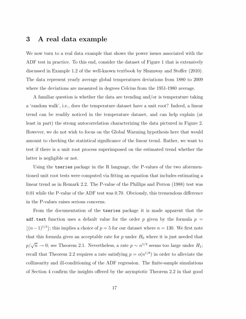
We now turn to a real data example that shows the power issues associated with the

ADF test in practice. To this end, consider the dataset of Figure 1 that is extensively

discussed in Example 1.2 of the well-known textbook by Shumway and Stoffer (2010).

The data represent yearly average global temperatures deviations from 1880 to 2009

where the deviations are measured in degrees Celcius from the 1951-1980 average.

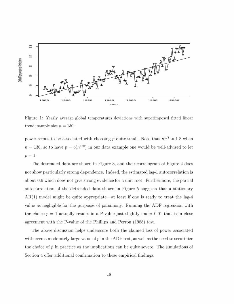
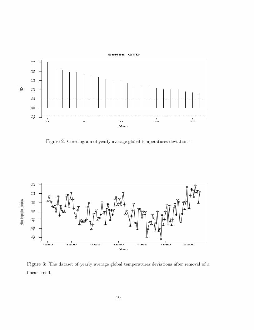
A familiar question is whether the data are trending and/or is temperature taking

a ‘random walk’, i.e., does the temperature dataset have a unit root? Indeed, a linear

trend can be readily noticed in the temperature dataset, and can help explain (at

least in part) the strong autocorrelation characterizing the data pictured in Figure 2.

However, we do not wish to focus on the Global Warming hypothesis here that would

amount to checking the statistical significance of the linear trend. Rather, we want to

test if there is a unit root process superimposed on the estimated trend whether the

latter is negligible or not.

Using the tseries package in the R language, the P-values of the two aforemen-

tioned unit root tests were computed via fitting an equation that includes estimating a

linear trend as in Remark 2.2. The P-value of the Phillips and Perron (1988) test was

0.01 while the P-value of the ADF test was 0.70. Obviously, this tremendous difference

in the P-values raises serious concerns.

From the documentation of the tseries package it is made apparent that the

adf.test function uses a default value for the order p given by the formula p =

b(n−1)1/3c; this implies a choice of p = 5 for our dataset where n = 130. We first note

that this formula gives an acceptable rate for p under H0 where it is just needed that

p/√

n → 0; see Theorem 2.1. Nevertheless, a rate p ∼ n1/3 seems too large under H1;

recall that Theorem 2.2 requires a rate satisfying p = o(n1/8) in order to alleviate the

collinearity and ill-conditioning of the ADF regression. The finite-sample simulations

of Section 4 confirm the insights offered by the asymptotic Theorem 2.2 in that good

17

1880 1900 1920 1940 1960 1980 2000

−0.4

−0.2

0.00.2

0.40.6

Year

Global

Temp

erature

Devia

tions

Figure 1: Yearly average global temperatures deviations with superimposed fitted linear

trend; sample size n = 130.

power seems to be associated with choosing p quite small. Note that n1/8 ≈ 1.8 when

n = 130, so to have p = o(n1/8) in our data example one would be well-advised to let

p = 1.

The detrended data are shown in Figure 3, and their correlogram of Figure 4 does

not show particularly strong dependence. Indeed, the estimated lag-1 autocorrelation is

about 0.6 which does not give strong evidence for a unit root. Furthermore, the partial

autocorrelation of the detrended data shown in Figure 5 suggests that a stationary

AR(1) model might be quite appropriate—at least if one is ready to treat the lag-4

value as negligible for the purposes of parsimony. Running the ADF regression with

the choice p = 1 actually results in a P-value just slightly under 0.01 that is in close

agreement with the P-value of the Phillips and Perron (1988) test.

The above discussion helps underscore both the claimed loss of power associated

with even a moderately large value of p in the ADF test, as well as the need to scrutinize

the choice of p in practice as the implications can be quite severe. The simulations of

Section 4 offer additional confirmation to these empirical findings.

18

0 5 10 15 20

−0.2

0.00.2

0.40.6

0.81.0

Year

ACF

Series GTD

Figure 2: Correlogram of yearly average global temperatures deviations.

1880 1900 1920 1940 1960 1980 2000

−0.3

−0.2

−0.1

0.00.1

0.20.3

Year

Global

Temp

erature

Devia

tions

Figure 3: The dataset of yearly average global temperatures deviations after removal of a

linear trend.

19

0 5 10 15 20

−0.2

0.00.2

0.40.6

0.81.0

Year

ACF

Series GTD.detrended

Figure 4: Correlogram of the detrended dataset of yearly average global temperatures devi-

ations.

5 10 15 20

−0.2

0.00.2

0.40.6

Year

Partial

ACF

Series GTD.detrended

Figure 5: Partial autocorrelation of the detrended dataset of yearly average global temper-

atures deviations.

20

4 A simulation experiment: good power vs. accu-

rate size

In order to complement our asymptotic results, as well as shed some light on the

unusual behavior of the ADF test on the real data example of Section 3, a numerical

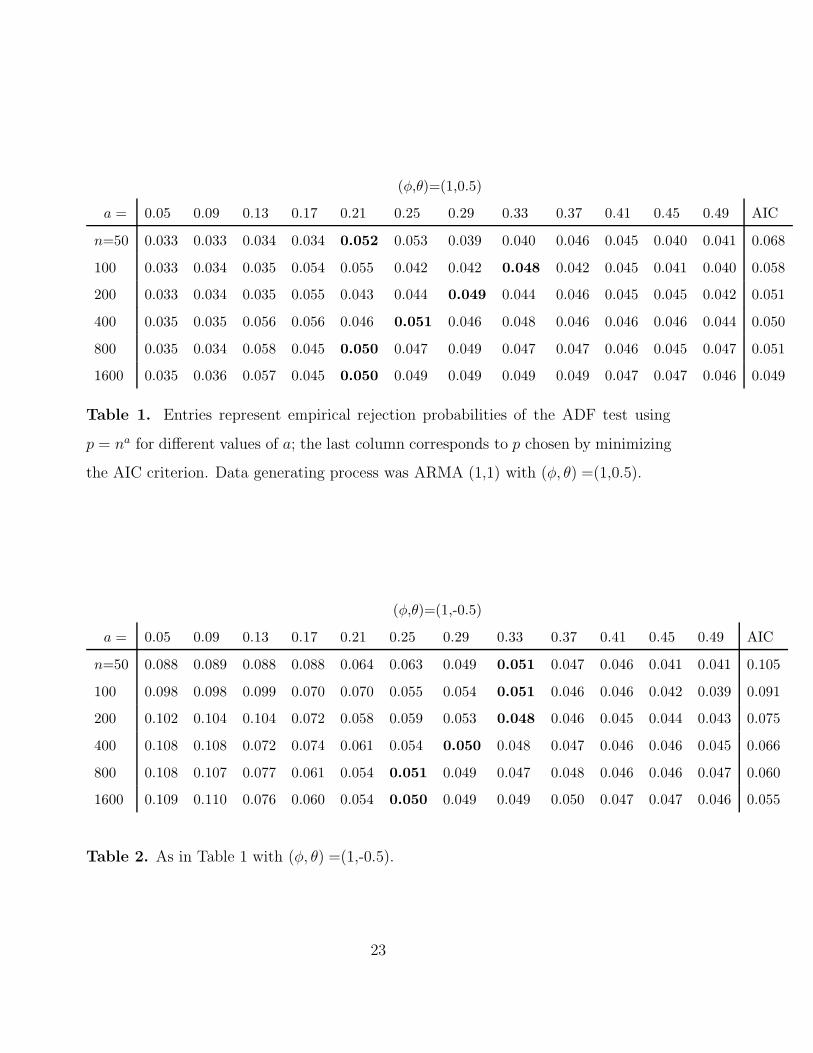
experiment was carried out. The data generating process was the ARMA (1,1) model:

Xt−φXt−1 = Zt+θZt−1 with Zt ∼ i.i.d. N(0, 1). For each of six different combinations

of the ARMA parameters φ and θ, and each sample size n, 100,000 time series of length

n were generated.

The simulation allowed us to compute empirical rejection probabilities of the ADF

test at nominal level 0.05; these are shown in Tables 1–6. In terms or the chosen order,

the formula p = na was used with a range of different values for a. The last column

from each Table corresponds to p chosen by minimizing the AIC criterion as detailed

in McLeod et al. (2012, p. 687); the AIC minimization was carried out over orders p

ranging from 1 to√

n.

Tables 1–2 concern the case where {Xt} has a unit root; hence, ideally all these

entries should be close to the nominal level 0.05. The entry closest to 0.05 in each row

is shown in boldface; for readability, the entries are rounded to three decimal points

but in case of ties more decimal points were used to pinpoint the optimal p. The

standard error of each of those entries is quite small, about 0.0007, hence the entries

give valuable and accurate information on the optimal p.

Putting the results of Tables 1–2 together, it seems that the formula p = na with

a ' 0.3 works very well for accurate size of the ADF test. Interestingly, although AIC

minimization gives generally good performance in the case of a positive MA parameter

θ, in the case of a negative θ it performs rather poorly except in the case of the huge

sample with n = 1600.

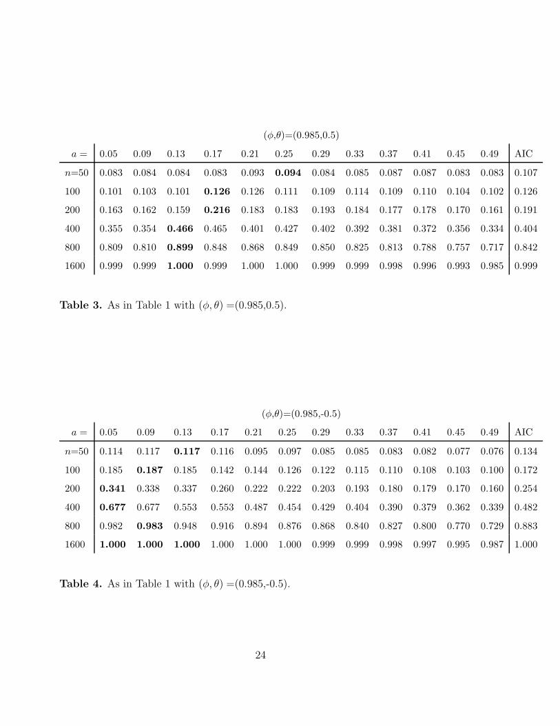
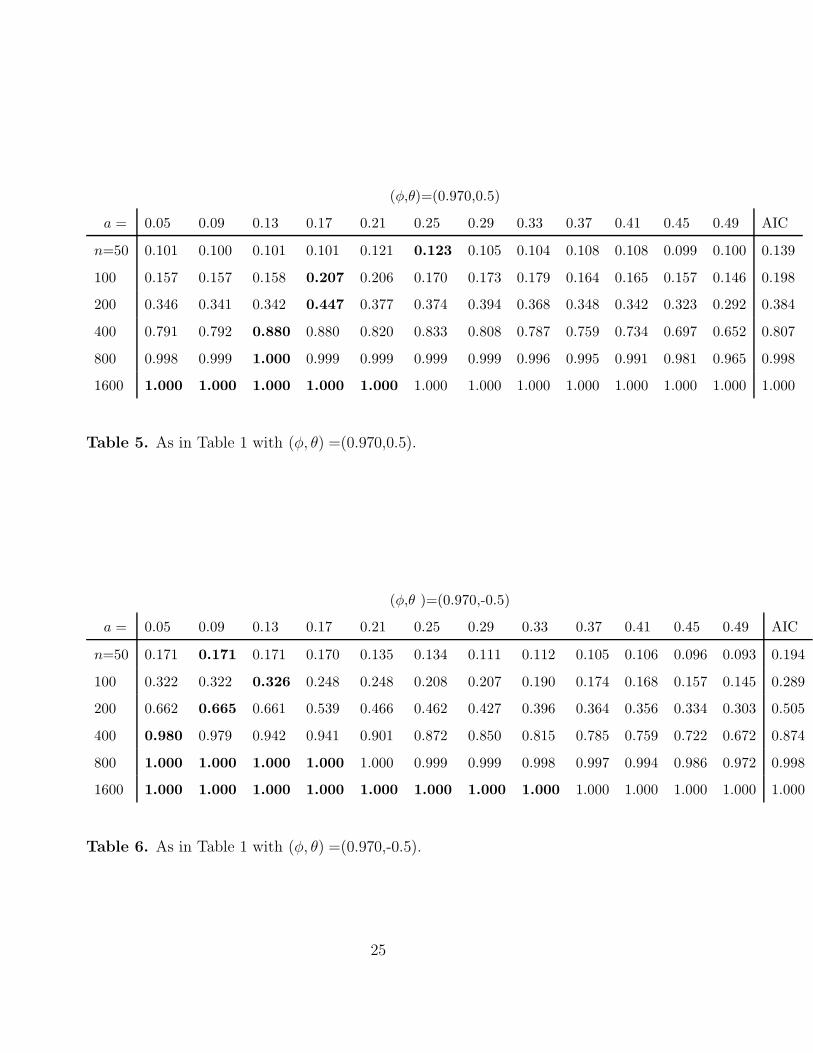
Tables 3–6 concern the case where {Xt} does not have a unit root, i.e., under the

21

alternative; hence, the entries represent power, and should be as big as possible. As

before, the biggest entries in each row are shown in boldface. The following conclusions

can be drawn.

• Finite-sample powers are in general quite low; nevertheless, power tends to one

as n increases. Therefore, the consistency of the test as claimed in Remark 2.5

is empirically verified.

• The p chosen to optimize size, i.e., p = n0.3, most definitely does not optimize

power.

• Even the formula p = na for some (other) constant a does not seem to work for

optimal power; if anything, Tables 3–6 seem to suggest power advantages when

using a formula of the type p = nan with an being a decreasing function of n.

• AIC minimization works reasonably well in terms of optimal power, in particular

in the case of positive MA parameter θ.

Remark 4.1 All in all, Tables 3–6 give empirical confirmation of the theoretical

treatment of Section 2 pointing out the need to use small orders p in order to increase

power and avoid collinearity. In addition, it is encouraging that AIC minimization

works well to optimize power. Unfortunately, the no-free-lunch principle seems to

apply here: implementing the ADF test using AIC minimization to chose the order

may lead to a test that has wrong size, namely over-rejecting under the null; see e.g.

Table 2.

22

(φ,θ)=(1,0.5)

a = 0.05 0.09 0.13 0.17 0.21 0.25 0.29 0.33 0.37 0.41 0.45 0.49 AIC

n=50 0.033 0.033 0.034 0.034 0.052 0.053 0.039 0.040 0.046 0.045 0.040 0.041 0.068

100 0.033 0.034 0.035 0.054 0.055 0.042 0.042 0.048 0.042 0.045 0.041 0.040 0.058

200 0.033 0.034 0.035 0.055 0.043 0.044 0.049 0.044 0.046 0.045 0.045 0.042 0.051

400 0.035 0.035 0.056 0.056 0.046 0.051 0.046 0.048 0.046 0.046 0.046 0.044 0.050

800 0.035 0.034 0.058 0.045 0.050 0.047 0.049 0.047 0.047 0.046 0.045 0.047 0.051

1600 0.035 0.036 0.057 0.045 0.050 0.049 0.049 0.049 0.049 0.047 0.047 0.046 0.049

Table 1. Entries represent empirical rejection probabilities of the ADF test using

p = na for different values of a; the last column corresponds to p chosen by minimizing

the AIC criterion. Data generating process was ARMA (1,1) with (φ, θ) =(1,0.5).

(φ,θ)=(1,-0.5)

a = 0.05 0.09 0.13 0.17 0.21 0.25 0.29 0.33 0.37 0.41 0.45 0.49 AIC

n=50 0.088 0.089 0.088 0.088 0.064 0.063 0.049 0.051 0.047 0.046 0.041 0.041 0.105

100 0.098 0.098 0.099 0.070 0.070 0.055 0.054 0.051 0.046 0.046 0.042 0.039 0.091

200 0.102 0.104 0.104 0.072 0.058 0.059 0.053 0.048 0.046 0.045 0.044 0.043 0.075

400 0.108 0.108 0.072 0.074 0.061 0.054 0.050 0.048 0.047 0.046 0.046 0.045 0.066

800 0.108 0.107 0.077 0.061 0.054 0.051 0.049 0.047 0.048 0.046 0.046 0.047 0.060

1600 0.109 0.110 0.076 0.060 0.054 0.050 0.049 0.049 0.050 0.047 0.047 0.046 0.055

Table 2. As in Table 1 with (φ, θ) =(1,-0.5).

23

(φ,θ)=(0.985,0.5)

a = 0.05 0.09 0.13 0.17 0.21 0.25 0.29 0.33 0.37 0.41 0.45 0.49 AIC

n=50 0.083 0.084 0.084 0.083 0.093 0.094 0.084 0.085 0.087 0.087 0.083 0.083 0.107

100 0.101 0.103 0.101 0.126 0.126 0.111 0.109 0.114 0.109 0.110 0.104 0.102 0.126

200 0.163 0.162 0.159 0.216 0.183 0.183 0.193 0.184 0.177 0.178 0.170 0.161 0.191

400 0.355 0.354 0.466 0.465 0.401 0.427 0.402 0.392 0.381 0.372 0.356 0.334 0.404

800 0.809 0.810 0.899 0.848 0.868 0.849 0.850 0.825 0.813 0.788 0.757 0.717 0.842

1600 0.999 0.999 1.000 0.999 1.000 1.000 0.999 0.999 0.998 0.996 0.993 0.985 0.999

Table 3. As in Table 1 with (φ, θ) =(0.985,0.5).

(φ,θ)=(0.985,-0.5)

a = 0.05 0.09 0.13 0.17 0.21 0.25 0.29 0.33 0.37 0.41 0.45 0.49 AIC

n=50 0.114 0.117 0.117 0.116 0.095 0.097 0.085 0.085 0.083 0.082 0.077 0.076 0.134

100 0.185 0.187 0.185 0.142 0.144 0.126 0.122 0.115 0.110 0.108 0.103 0.100 0.172

200 0.341 0.338 0.337 0.260 0.222 0.222 0.203 0.193 0.180 0.179 0.170 0.160 0.254

400 0.677 0.677 0.553 0.553 0.487 0.454 0.429 0.404 0.390 0.379 0.362 0.339 0.482

800 0.982 0.983 0.948 0.916 0.894 0.876 0.868 0.840 0.827 0.800 0.770 0.729 0.883

1600 1.000 1.000 1.000 1.000 1.000 1.000 0.999 0.999 0.998 0.997 0.995 0.987 1.000

Table 4. As in Table 1 with (φ, θ) =(0.985,-0.5).

24

(φ,θ)=(0.970,0.5)

a = 0.05 0.09 0.13 0.17 0.21 0.25 0.29 0.33 0.37 0.41 0.45 0.49 AIC

n=50 0.101 0.100 0.101 0.101 0.121 0.123 0.105 0.104 0.108 0.108 0.099 0.100 0.139

100 0.157 0.157 0.158 0.207 0.206 0.170 0.173 0.179 0.164 0.165 0.157 0.146 0.198

200 0.346 0.341 0.342 0.447 0.377 0.374 0.394 0.368 0.348 0.342 0.323 0.292 0.384

400 0.791 0.792 0.880 0.880 0.820 0.833 0.808 0.787 0.759 0.734 0.697 0.652 0.807

800 0.998 0.999 1.000 0.999 0.999 0.999 0.999 0.996 0.995 0.991 0.981 0.965 0.998

1600 1.000 1.000 1.000 1.000 1.000 1.000 1.000 1.000 1.000 1.000 1.000 1.000 1.000

Table 5. As in Table 1 with (φ, θ) =(0.970,0.5).

(φ,θ )=(0.970,-0.5)

a = 0.05 0.09 0.13 0.17 0.21 0.25 0.29 0.33 0.37 0.41 0.45 0.49 AIC

n=50 0.171 0.171 0.171 0.170 0.135 0.134 0.111 0.112 0.105 0.106 0.096 0.093 0.194

100 0.322 0.322 0.326 0.248 0.248 0.208 0.207 0.190 0.174 0.168 0.157 0.145 0.289

200 0.662 0.665 0.661 0.539 0.466 0.462 0.427 0.396 0.364 0.356 0.334 0.303 0.505

400 0.980 0.979 0.942 0.941 0.901 0.872 0.850 0.815 0.785 0.759 0.722 0.672 0.874

800 1.000 1.000 1.000 1.000 1.000 0.999 0.999 0.998 0.997 0.994 0.986 0.972 0.998

1600 1.000 1.000 1.000 1.000 1.000 1.000 1.000 1.000 1.000 1.000 1.000 1.000 1.000

Table 6. As in Table 1 with (φ, θ) =(0.970,-0.5).

25

5 Technical Proofs

Proof of Theorem 2.1: Using the notation ∆Xt,p = (∆Xt, ∆Xt−1, . . . , ∆Xt−p+1)′

,

εt,p = Xt −ρXt−1−∑p

j=1 aj,p∆Xt−j and εt,p = Xt − ρnXt−1 −∑p

j=1 aj,p∆Xt−j with least

squares estimators ρn and aj,p, j = 1, 2, . . . , p, it is easily verified that

tn = (ρn − 1)/Std(ρn) = LnR−1n /(σ2

nR−1n )1/2,

where

Ln =n∑

t=p+1

Xt−1εt,p − (n∑

t=p+1

Xt−1∆X′

t−1,p)(n∑

t=p+1

∆Xt−1,p∆X′

t−1,p)−1(

n∑

t=p+1

∆Xt,pεt,p),

(5.11)

Rn =n∑

t=p+1

X2t−1 − (

n∑

t=p+1

Xt−1∆X′

t−1,p)(n∑

t=p+1

∆Xt−1,p∆X′

t−1,p)−1

(n∑

t=p+1

∆Xt,pXt−1)

(5.12)

and σ2n = (n−p)−1 ∑n

t=p+1 ε2t,p is the error variance estimator. Now, for i, j ∈ {1, 2, . . . , p}

we have that, as n → ∞, n−1 ∑nt=p+1 ∆Xt−i∆Xt−j → γU(i−j) in probability, and that,

by the same arguments as in Berk (1974), p.493,

‖n−1n∑

t=p+1

∆Xt−1,p∆X′

t−1,p‖ = OP (1), (5.13)

where for a matrix C , the norm ‖C‖ = sup‖x‖≤1 ‖Cx‖ is used and ‖x‖ denotes the

Euclidean norm of the vector x. Furthermore,

1

np1/2‖

n∑

t=p+1

∆Xt−1,pXt−1‖ =(p−1

p∑

j=1

(n−1n∑

t=p+1

∆Xt−jXt−1)2)1/2

= OP (1) (5.14)

since n−1 ∑nt=p+1 ∆Xt−jXt−1 = n−1 ∑n

t=p+1

∑t−1l=1 Ut−jUl = OP (1). Finally, since

n−1/2 ∑nt=p+1 ∆Xt−jεt,p = n−1/2 ∑n

t=p+1 Ut−jεt,p = OP (1) we get that

√p n−1‖

n∑

t=p+1

∆Xt−1,pεt,p‖ =p√n

(p−1

p∑

j=1

(1√n

n∑

t=p+1

∆Xt−jεt,p)2)1/2

=p√n

OP (1) → 0 (5.15)

26

as n → ∞. Now, equations (5.13) to (5.15) implies that n−1Ln = n−1 ∑nt=p+1 Xt−1εt,p+

oP (1). Furthermore, because

n−1n∑

t=p+1

Xt−1(εt,p − εt) =p∑

j=1

(aj,p − aj)n−1

n∑

t=p+1

Xt−1Ut−j +∞∑

j=p+1

ajn−1

n∑

t=p+1

Xt−1Ut−j ,

if follows using n−1 ∑nt=p+1 Xt−1Ut−j = OP (1) and Baxter’s inequality, cf. Lemma 2.2

of Kreiss et al. (2011), that

|n−1n∑

t=p+1

Xt−1(εt,p − εt)| ≤ OP (∞∑

j=p+1

|aj|) → 0,

as p → ∞. Thus,

n−1Ln = n−1n∑

t=p+1

Xt−1εt + oP (1). (5.16)

Similarly, using (5.13) and (5.14) we obtain that

n−2Rn = n−2n∑

t=p+1

X2t−1 + oP (1). (5.17)

Now, as in the proof of Theorem 3.1 in Phillips (1987) and using the invariance

principle for the partial sum process S[nr] = n−1/2 ∑[nr]j=1 εj of zero mean weakly depen-

dent random variables satisfying Assumption 1(ii), established in Theorem 1 of Wu

and Min (2005), we get that

n−1Ln ⇒ σ2ε

∫ 1

0W (t)dW (t), and n−2Rn ⇒ σ2

ε

∫ 1

0W 2(t)dt.

2

Proof of Proposition 2.1: Let δj,p, j = 0, 1, . . . , p be the coefficients of ∆Xt−j in the

best linear prediction of Xt based on ∆Xt−j and define lj,p = (1− j/p), j = 0, 1, . . . , p.

We have

E(Xt − PMt,t−pXt)

2 = E(Xt −p∑

j=0

lj,p∆Xt−j)2 + E(

p∑

j=0

(lj,p − δj,p)∆Xt−j)2

−2E(p∑

j=0

(lj,p − δj,p)∆Xt−j)(Xt −p∑

j=0

lj,p∆Xt−j).

27

Note first that E(Xt −∑p

j=0 lj,p∆Xt−j)2 = p−1[γ(0) + 2

∑p−1s=1(1 − s/p)γ(s)], which

converges to zero if γ(h) → 0. Furthermore, if∑∞

h=−∞ |γ(h)| < ∞ then p · E(Xt −∑p

j=0 lj,p∆Xt−j)2 → ∑∞

h=−∞ γ(h) = 2πfXt(0) by the dominate convergence theorem.

Now, let Xt(p) = (Xt, Xt−1, . . . , Xt−p)′

, Γp+1 = E(Xt(p)Xt(p)′

) and define the (p + 1)-

dimensional vectors δ(p) = ((1 − δ0,p), (δ0,p − δ1,p), . . . , (δp−1,p − δp,p), δp,p) and l(p) =

(0, 1/p, 1/p, . . . , 1/p, 0)′

. Then the following upper bound is valid,

E(p∑

j=0

(lj,p − δj,p)∆Xt−j)2 = (l(p) − δ(p))

′

Γp+1(l(p) − δ(p))

≤ maxλ∈[0,π]

fXt(λ)‖l(p) − δ(p)‖2

≤ maxλ∈[0,π]

fXt(λ)

(2‖l(p)‖2 + 2‖δ(p)‖2

).

It is easily seen that ‖l(p)‖2 = O(p−1) → 0. Furthermore, using the following lower

bound for the mean square prediction error

E(Xt − PMt,t−pXt)

2 =∫ π

−π|

p∑

j=0

δj,pe−ijλ|2fXt

(λ)dλ ≥ infλ∈[0,π]

fXt(λ)‖δ(p)‖2,

we get that ‖δ(p)‖2 → 0 as p → ∞ from which it follows that E(∑p

j=0(lj,p−δj,p)∆Xt−j)2 →

0 as p → 0. Finally, by the above results and Cauchy-Schwarz’s inequality, it follows

that |E(∑p

j=0(lj,p − δj,p)∆Xt−j)(Xt −∑p

j=0 lj,p∆Xt−j)| → 0 which concludes the proof.

2

Proof of Theorem 2.2: Note that√

n/p (ρn − ρ) =√

n/p LnR−1n where Ln and Rn

are defined in (5.11) and (5.12). Let γ0 = (n − p)−1 ∑nt=p+1 X2

t−1,

dp =( 1

n − p

n∑

t=p+1

∆Xt−iXt−1, i = 1, 2, . . . , p)′

, and Cp =( 1

n − p

n∑

t=p+1

∆Xt−i∆Xt−j

)i,j=1,2,...,p

.

We have that

n−1Rn = γ0 − d′

pC−1p dp

= γ0 − d′

pC−1p dp + OP (p3/n1/2), (5.18)

28

where d′

p = (E(Xt−1∆Xt−j), j = 1, 2, . . . , p) and Cp = E(∆Xt−1,p∆X′

t−1,p). Notice

that the OP (p3/n1/2) term in (5.18) appears because using the notation τ 2p = γ0 −

d′

pC−1p dp and τ 2

p = γ0 − d′

pC−1p dp, we have that

|τ 2p − τ 2

p | ≤ |γ0 − γ0| + ‖δp − δp‖‖dp‖ + ‖dp − dp‖‖δp‖

where δp = C−1p dp and δp = C−1

p dp. Now, ‖dp − dp‖ = OP (p1/2/n1/2) and

p−1/2‖dp‖ = {p−1p∑

j=1

((n − p)−1n∑

t=p+1

∆Xt−jXt−1)2}1/2 = OP (1).

Furthermore,

‖δp − δp‖ = OP (p5/2/n1/2), (5.19)

and

p−1‖δp‖ = oP (1), (5.20)

which implies that |τ 2p − τ 2

p | = OP (p3/n1/2). We show that (5.19) and (5.20) are true.

To see (5.19) notice first that

δp − δp = C−1p ((n − p)−1

n∑

t=p+1

∆Xt−1,put−1,p),

where ut−1,p = Xt−1 −∑p

j=1 δj,p∆Xt−j and δp = (δ1,p, δ2,p, . . . , δp,p) are the coefficients

of the best linear predictor of Xt−1 based on ∆Xt−j , j = 1, 2, . . . , p. Now,

‖δp − δp‖ ≤ ‖C−1p ‖‖(n − p)−1

n∑

t=p+1

∆Xt−1,put−1,p‖ = OP (p5/2/n1/2),

since ‖(n − p)−1 ∑nt=p+1 ∆Xt−1,put−1,p‖ = OP (p1/2/n1/2), and

‖C−1p ‖ = OP (p2). (5.21)

To see why (5.21) is true notice that for every p ∈ IN the matrix Cp is positive definite,

‖C−1p ‖ is the reciprocal of the minimal eigenvalue of Cp. Notice that the spectral density

29

f∆Xt(λ) of the differenced process {∆Xt, t ∈ ZZ} satisfies f∆Xt

(λ) = |1 − eiλ|2fXt(λ)

and that for the minimal eigenvalue of Cp we have

inf‖x‖=1

p∑

j=1

p∑

k=1

xjCov(∆Xt−j , ∆Xt−k)xk = inf‖x‖=1

1

2π

∫ π

−π

∣∣∣p∑

j=1

xjeijλ

∣∣∣2fXt

(λ)|1 − eiλ|2dλ

≥ infλ∈[0,π]

fXt(λ) inf

‖x‖=1

1

2π

∫ π

−π

∣∣∣p∑

j=1

xjeijλ

∣∣∣2|1 − eiλ|2dλ

= infλ∈[0,π]

fXt(λ)λmin,

where λmin denotes the minimal eigenvalue of the p×p covariance matrix of the process

with spectral density (2π)−1|1 − eiλ|2 = (2π)−12(1 − cos(λ)), i.e. of the noninvertible

MA(1) process Yt = εt − εt−1. For this process the eigenvalues of the p-dimensional

correlation matrix are given by λk = 2(1 − cos((kπ)/(p + 1))), k = 1, 2, . . . , p. Thus,

‖C−1p ‖ ≤ 1/K(1 − cos(π/(p + 1))) = O(p2), where the last equality follows because

[1 − cos(π/(p + 1))] ∼ p−2. Note that ‖C−1p ‖ → ∞ as p → ∞ since the minimal

eigenvalue of Cp approaches zero as p → ∞. Furthermore, it is easily seen that ‖Cp −Cp‖ = OP (p/

√n) from which we get using ‖C−1

p ‖ = O(p2) that

‖C−1p − C−1

p ‖ ≤ ‖C−1p ‖2‖Cp − Cp‖

1 − ‖Cp − Cp‖‖C−1p ‖

= OP (p5/2/n1/2).

Thus,

‖C−1p ‖ ≤ ‖C−1

p ‖ + ‖C−1p − C−1

p ‖ = OP (p2 + p5/2/n1/2).

To see (5.20) notice that

‖δp‖ ≤ ‖δp‖ + ‖δp − δp‖.

Now, ‖δp − δp‖ = OP (p5/2/n1/2). Furthermore, for lp = (l1,p, l2,p, . . . , lp,p)′

, lj,p =

(1 − j/p), j = 1, 2, . . . , p we have ‖δp‖ ≤ ‖lp‖ + ‖δp − lp‖. Now, ‖lp‖ = O(√

p) while

‖lp − δp‖ = o(p) which follows because

(lp − dp)′

Cp(lp − dp) ≥ λmin‖lp − δp‖2

≥ infλ∈[0,π]

fXt(λ)2(1 − cos(π/(p + 1))‖lp − dp‖2

∼ Kp−2‖lp − δp‖2 ≥ 0,

30

and as the proof of Proposition 2.1 shows (lp − dp)′

Cp(lp − dp) = E(∑p

j=0(lj,p −δj,p)∆Xt−j)

2 → 0, as p → ∞.

This concludes the proof of assertion (5.18).

Now,

pτ 2p → 2πfXt

(0) = σ2ε(1 − ρ)

−2, (5.22)

by Proposition 2.1. Thus

p

nRn = σ2

ε(1 − ρ)−2 + OP (p4/n1/2). (5.23)

Let Vt−1,p =√

p(Xt−1 − d′

pC−1p ∆Xt−1,p) and Vt−1,p =

√p(Xt−1 − d

′

pC−1p ∆Xt−1,p).

Then,

√p

nLn =

1√n

n∑

t=p+1

Vt−1,pεt,p

=1√n

n∑

t=p+1

Vt−1,pεt +1√n

n∑

t=p+1

(Vt−1,p − Vt−1,p)εt

+1√n

n∑

t=p+1

Vt−1,p(εt,p − εt)

=1√n

n∑

t=p+1

Vt−1,pεt + L1,n + L2,n,

with an obvious notation for the remainder terms L1,n and L2,n. For these terms we

have

|L1,n| ≤ √p‖δp − δp‖‖n−1/2

n∑

t=p+1

∆Xt−1,pεt‖

= OP (p7/2/n1/2) → 0 as n → ∞.

and

|L2,n| ≤ (n−1n∑

t=p+1

V 2t−1,p)

1/2(n∑

t=p+1

(εt,p − εt)2)1/2

= OP (√

nn∑

j=p+1

|aj|).

31

Notice that the last equality above follows since under the assumptions made,

n−1n∑

t=p+1

V 2t−1,p = n−1

n∑

t=p+1

p(Xt−1 − δ′

p∆Xt−1,p)2 + oP (1) = OP (1),

and by Baxter’s inequality, see Kreiss et al. (2011), Lemma 2.2,

E(n∑

t=p+1

(εt,p − εt)2) = O(

√n

∞∑

j=p+1

|aj|).

The proof of the theorem is then concluded since under the assumptions made and by

a central limit theorem for martingale differences, see Theorem 1 of Brown(1971),

1√n

n∑

t=p+1

Vt−1,pεt ⇒ N(0, σ4ε(1 − ρ)−2). (5.24)

2

References

[1] Abadir, K. M. (1993), On the Asymptotic Power of Unit Root Tests. EconometricTheory, 9, 189-221.

[2] Berk, K. (1974), Consistent Autoregressive Spectral Estimates. Annals of Statis-tics, 2, 489-502.

[3] Breitung, J. (2002). Nonparametric tests for unit roots and cointegration. Journalof Econometrics, 108, 343-363

[4] Brown, B. M. (1971), Martingale Central Limit Theorems. Annals of Mathemat-ical Statistics, 42, 59-66.

[5] Chang, Y. and J. Y. Park (2002), On the Asymptotics of ADF Tests for UnitRoots. Econometric Reviews, 21, 431-447.

[6] Dickey, D. A. and Fuller, W. A. (1979), Distribution of Estimators for Autore-gressive Time Series with a Unit Root. Journal of the American Statistical As-sociation, 74, 427-431.

[7] Dickey, D. A. and Fuller. W. A. (1981), Likelihood Ratio Statistics for Autore-gressive Time Series with a Unit Root. Econometrica, 49, 1057-1072.

[8] Elliott, G., Rothenberg T. J. and Stock, J. H. (1996). Efficient tests on an au-toregressive unit root. Econometrica, 64, 813-836

[9] Hamilton, J.D. (1994). Time Series Analysis, Princeton University Press.

32

[10] Harvey, D. I., Leybourne, S. J. and Taylor, A. M. R. (2009). Unit root test-ing in practice: dealing with uncertainity over the trend and initial condition.Econometric Theory, 25, 587-636.

[11] Kreiss, J. P., E. Paparoditis and D. N. Politis (2011), On the Range of Validityof the Autoregressive Sieve Bootstrap. Annals of Statistics, 39, 2103-2130.

[12] Kwiatkowski, D., Phillips, P.C.B., Schmidt, P. and Shin, Y. (1992). Testing thenull hypothesis of stationarity against the alternative of a unit root: How sureare we that economic time series have a unit root? Journal of Econometrics, 54,159-178.

[13] Lopez, J. H. (1997), The Power of the ADF Test. Economics Letters, 57, 5-10.

[14] McLeod, I.A., Yu, H., and Mahdi, M. (2012). Time series analysis with R, inTime Series Analysis: Methods and Applications, vol. 30, (T. Subba Rao et al.,Eds.), pp. 661–712, Amsterdam: Elsevier.

[15] Muller, U.K. (2005), Size and Power of Tests of Stationarity in Highly Autocor-related Time Series, Journal of Econometrics, 128, 195 213.

[16] Muller, U.K. (2007), A theory for robust long-run variance estimation, Journalof Econometrics, 141, 1331-1352.

[17] Muller, U.K. and Elliott, G. (2003), Tests for unit roots and the initial condition,Econometrica, 71, 1269-1286.

[18] Muller, U.K. and Watson M. W. (2008), Testing models of low-frequency vari-ability. Econometrica, 76, 979-1016.

[19] Nabeya, S. and Tanaka, K. (1990), A General Approach to the Limiting Distri-bution for Estimators in Time Series Regression with Nonstable AutoregressiveErrors. Econometrica, 58, 145-163.

[20] Ng, S. and P. Perron (1995), Unit Root Tests in ARMA Models with Data-Dependent Methods for the Selection of the Truncation Lag. Journal of theAmerican Statistical Association, 90, 268-281.

[21] Nielsen, M. Ø. (2009). A powerful test of the autoregressive unit root hypothesisbased on a tuning parameter free statistic. Econometric Theory, 25, 1515-1544.

[22] Patterson, K. (2011), Unit Root Tests in Time Series, Vol. I, Palgrave Texts inEconometrics, Palgrave Macmillan, Hampshire, U.K.

[23] Pourahmadi, M. (2001), Foundations of Time Series Analysis and PredictionTheory, John Wiley, New York.

[24] Perron, P. (1991), A Continous Time Approximation to the Unstable First-OrderAutoregressive Process: The Case Without an Intercept. Econometrica, 59, 211-236.

33

[25] Phillips, P. C. B. (1987), Time Series Regression with a Unit Root. Econometrica,2, 277-301.

[26] Phillips, P. C. B. and P. Perron (1988), Testing for a Unit Root in Time SeriesRegression. Biometrika, 75, 335-346.

[27] Said, S. E. and S. A. Dickey (1984), Testing for Unit Roots in Autoregressive-Moving Average Models of Unknown Order. Biometrika, 71, 599-607.

[28] Shin, Y. and Schmidt, P. (1992). The KPSS stationarity test as a unit root test.Economics Letters, 38, 387-392

[29] Shumway, R.H. and Stoffer, D.S. (2010). Time Series Analysis and Its Applica-tions: With R Examples, 3rd Ed., Springer, New York.

[30] Wu, B. W. (2005), Nonlinear System Theory: Another look at Dependence. Proc.Nat. Journal Acad. Sci. USA, 102, 14150-14154.

[31] Wu, B. W. and Min, W. (2005), On Linear Processes with Dependent Innova-tions. Stochastic Processes and their Applications, 115, 939-958.

34