The Armchair Celestial Navigator

Concepts, Math, the Works, but Different

Rodger E. Farley

1

Contents Preface Variable and Acronym List Chapter 1 Early Related History Chapter 2 Review of Fundamentals Chapter 3 Celestial Navigation Concepts Chapter 4 Calculations for Lines of Position Chapter 5 Measuring Altitude with the Sextant Chapter 6 Corrections to Measurements Chapter 7 Reading the Nautical Almanac Chapter 8 Sight Reduction Chapter 9 Putting it Together and Navigating Chapter 10 Star Identification Chapter 11 Special Topics Chapter 12 Lunars Chapter 13 Coastal Navigation using the sextant Appendix 1 Compendium of Equations Appendix 2 Making your very own Octant Copyright 2002 Rodger E. Farley Unpublished work. All rights reserved. My web site: http://mysite.verizon.net/milkyway99/index.html

2

Preface

Growing up, I had always been fascinated by the thought of navigating by the stars. However, it instinctively seemed to me an art beyond my total understanding. Why, I don’t know other than celestial navigation has always had a shroud of mystery surrounding it, no doubt to keep the hands from mutiny. Some time in my 40s, I began to discard my preconceived notions regarding things that required ‘natural’ talent, and thus I began a journey of discovery. This book represents my efforts at teaching myself ‘celestial’, although it is not comprehensive of all my studies in this field. Like most educational endeavors, one may sometimes plunge too deeply in seeking arcane knowledge, and risk loosing the interest and attention of the reader. With that in mind, this book is dedicated simply to removing the cloak of mystery; to teach the concepts, some interesting history, the techniques, and computational methods using the simple pocket scientific calculator. And yes, also how to build your own navigational tools. My intention is for this to be used as a self-teaching tool for those who have a desire to learn celestial from the intuitive, academic, and practical points of view. This book should also interest experienced navigators who are tired of simply ‘turning the crank’ with tables and would like a better behind-the-scenes knowledge. With the prevalence of hand electronic calculators, the traditional methods of using sight-reduction tables with pre-computed solutions will hardly be mentioned here. I am referring to the typical Hydrographic Office methods H.O. 249 and H.O. 229. Rather, the essential background and equations to the solutions will be presented such that the reader can calculate the answers precisely with a hand calculator and understand the why. You will need a scientific calculator, those having trigonometric functions and their inverse functions. Programmable graphing calculators such as the TI-86 and TI-89 are excellent for the methods described in the book. To those readers familiar with ‘celestial’, they will notice that I have departed the usual norms found in celestial navigation texts. I use a consistent sign convention which allows me to discard same-name and opposite-name rules.

Rodger Farley 2002

3

Variable and Acronym List Hs Altitude angle as reported on the sextant scale Ha Apparent altitude angle Ho Observed, or true altitude angle Hc Calculated altitude angle IC Index correction SD Angular semi-diameter of sun or moon UL Upper limb of sun or moon LL Lower limb of sun or moon GHA Greenwich hour angle GHAhour Greenwich hour angle as tabulated at a specific integer hour DEC Declination angle DEChour Declination angle as tabulated at a specific integer hour SHA Sidereal hour angle LHA Local hour angle Zo Uncorrected azimuth angle Zn Azimuth angle from true north v Hourly variance from the nominal GHA rate, arcmin per hour d Hourly declination rate, arcmin per hour heye Eye height above the water, meters CorrDIP Correction for dip of the horizon due to eye height Corrv Correction to the tabular GHA for the variance v Corrd Correction to the tabular declination using rate d CorrGHA Correction to the tabular GHA for the minutes and seconds CorrALT Correction to the sextant altitude for refraction, parallax, and

semidiameter R Correction for atmospheric refraction Doffset Offset distance using the intercept method, nautical miles LAT Latitude LON Longitude LATA Assumed latitude LONA Assumed longitude LATDR Estimated latitude, or dead-reckoning latitude LONDR Estimated longitude, or dead-reckoning longitude LOP Line of position LAN Local apparent noon LMT Local mean time

4

Chapter One

Early Related History Why 360 degrees in a circle? If you were an early astronomer, you would have noticed that the stars rotate counterclockwise (ccw) about Polaris at the rate of seemingly once per day. And that as the year moved on, the constellation’s position would slowly crank around as well, once per year ccw. The planets were mysterious, and thought to be gods as they roamed around the night sky, only going thru certain constellations, named the zodiac (in the ecliptic plane). You would have noticed that after ¼ of a year had passed, or ~ 90 days, that the constellation had turned ccw about ¼ of a circle. It would have seemed that the angle of rotation per day was 1/90 of a quarter circle. A degree could be thought of as a heavenly angular unit, which is quite a coincidence with the Babylonian base 60 number system which established the angle of an equilateral triangle as 60º.

The Egyptians had divided the day into 24 hours, and the Mesopotamians further divided the hour into 60 minutes, 60 seconds per minute. It is easy to see the analogy between angle and clock time, since the angle was further divided into 60 arcminutes per degree, and 60 arcseconds per arcminute. An arcminute of arc length on the surface of our planet defined the unit of distance; a nautical mile, which = 1.15 statute miles. By the way, mile comes from the Latin milia for 1000 double paces of a Roman soldier. Size of the Earth In the Near East during the 3rd century BC lived an astronomer-philosopher by the name of Eratosthenes, who was the director of the Egyptian Great Library of Alexandria. In one of the scroll books he read that on the summer solstice June 21 in Syene (south of Alexandria), that at noon vertical sticks would cast no shadow (it was on the tropic of Cancer). He wondered that on the same day in Alexandria, a stick would cast a measurable shadow. The ancient Greeks had hypothesized that the earth was round, and this observation by Eratosthenes confirmed the curvature of the Earth. But how big was it? On June 21 he measured the angle cast by the stick and saw that it was approximately 1/50th of a full circle (7 degrees). He hired a man to pace out the distance between Alexandria and Syene, who reported it was 500 miles. If 500 miles was the arc length for 1/50 of a huge circle, then the Earth’s circumference would be 50 times longer, or 50 x 500 = 25000 miles. That was quite an accurate prediction with simple tools for 2200 years ago.

5

Calendar Very early calendars were based on the lunar month, 29 ½ days. This produced a 12-month year with only 354 days. Unfortunately, this would ‘drift’ the seasons backwards 11 ¼ days every year according to the old lunar calendars. Julius Caesar abolished the lunar year, used instead the position of the sun and fixed the true year at 365 ¼ days, and decreed a leap day every 4 years to make up for the ¼ day loss per Julian year of 365 days. Their astronomy was not accurate enough to know that a tropical year is 365.2424 days long; 11 minutes and 14 seconds shorter than 365 ¼ days. This difference adds a day every 128.2 years, so in 1582, the Gregorian calendar was instituted in which 10 days that particular October were dropped to resynchronize the calendar with the seasons, and 3 leap year days would not be counted every 400 years to maintain synchronicity. Early Navigation The easiest form of navigating was to never leave sight of the coast. Species of fish and birds, and the color and temperature of the water gave clues, as well as the composition of the bottom. When one neared the entrance to the Nile on the Mediterranean, the bottom became rich black, indicating that you should turn south. Why venture out into the deep blue water? Because of coastal pirates, and storms that pitch your boat onto a rocky coast. Presumably also to take a shorter route. One could follow flights of birds to cross the Atlantic, from Europe to Iceland to Greenland to Newfoundland. In the Pacific, one could follow birds and know that a stationary cloud on the horizon meant an island under it. Polynesian navigators could also read the swells and waves, determine in which direction land would lie due to the interference in the wave patterns produced by a land mass. And then there are the stars. One in particular, the north pole star, Polaris. For any given port city, Polaris would always be more or less at a constant altitude angle above the horizon. Latitude hooks, the kamal, and the astrolabe are ancient tools that allowed one to measure the altitude of Polaris. So long as your last stage of sailing was due east or west, you could get back home if Polaris was at the same altitude angle as when you left. If you knew the altitude angle of Polaris for your destination, you could sail north or south to pick up the correct Polaris altitude, then ‘run down the latitude’ until you arrive at the destination. Determining longitude would remain a mystery for many ages. Techniques used in surveying were adopted for use in navigation, two of which are illustrated on the next page.

6

‘Running down the latitude’ from home to destination, Trade wind sailing following changing latitude where safe to pick up trade winds separate latitudes

Surveying techniques with absolute angles and relative angles

7

Chapter Two

Review of Fundamentals Orbits The Earth’s orbit about the Sun is a slightly elliptical one, with a mean distance from the Sun equal to 1 AU (AU = Astronomical Unit = 149,597,870. km). This means that the Earth is sometimes a little closer and sometimes a little farther away from the Sun than 1 AU. When it’s closer, it is like going down hill where the Earth travels a little faster thru it’s orbital path. When it’s farther away, it is like going up hill where the Earth travels a little slower. If the Earth’s orbit were perfectly circular, and was not perturbed by any other body (such as the Moon, Venus, Mars, or Jupiter), in which case the orbital velocity would be unvarying and it could act like a perfect clock. This brings us to the next topic… Mean Sun The mean Sun is a fictional Sun, the position of the Sun in the sky if the Earth’s axis was not tilted and its orbit were truly circular. We base our clocks on the mean Sun, and so the mean Sun is another way of saying the year-averaged 24 hour clock time. This leads to the situation where the true Sun is up to 16 minutes too fast or 14 minutes too slow from clock reckoning. This time difference between the mean Sun and true Sun is known as the Equation of Time. The Equation of Time at local noon is noted in the Nautical Almanac for each day. For several months at a time, local noon of the true Sun will be faster or slower than clock noon due to the combined effects of Earth’s tilt angle and orbital velocity. When we graph the Equation of Time in combination with the Sun’s declination angle, we produce a shape known as the analemma. The definition and

8

significance of solar declination will be explained in a later section. Time With a sundial to tell us local noon, and the equation of time to tell us the difference between solar and mean noon, a simple clock could always be reset daily. We think we know what we mean when we speak of time, but how to measure it? If we use the Earth as a clock, we could set up a fixed telescope pointing at the sky due south with a vertical hair line in the eyepiece and pick a guide star that will pass across the hairline. After 23.93 hours (a sidereal day, more later) from when the guide star first crossed the hairline, the star will pass again which indicates that the earth has made a complete revolution in inertial space. Mechanical clocks could be reset daily according to observations of these guide stars. A small problem with this reasonable approach is that the Earth’s spin rate is not completely steady, nor is the direction of the Earth’s spin axis. It was hard to measure, as the Earth was our best clock, until atomic clocks showed that the Earth’s rate of rotation is gradually slowing down due mainly to tidal friction, which is a means of momentum transference between the Moon and Earth. Thus we keep fiddling with the definition of time to fit our observations of the heavens. But orbital calculations for planets and lunar positions (ephemeris) must be based on an unvarying absolute time scale. This time scale that astronomers use is called Dynamical Time. Einstein of course disagrees with an absolute time scale, but it is relative to Earth’s orbital speed. Time Standards for Celestial Navigation Universal Time (UT, solar time, GMT) This standard keeps and resets time according to the mean motion of the Sun across the sky over Greenwich England, the prime meridian, (also known as Greenwich Mean Time GMT). UT is noted on a 24-hour scale, like military time. The data in the nautical almanac is based on UT. Universal Time Coordinated (UTC) This is the basis of short wave radio broadcasts from WWV in Fort Collins Colorado and WWVH in Hawaii (2.5, 5,10,15,20 MHz). It is also on a 24-hour scale. It is synchronized with International Atomic Time, but can be an integral number of seconds off in order to be coordinated with UT such that it is no more than 0.9 seconds different from UT. Initial calibration errors when the atomic second was being defined in the late 1950’s, along with the gradual slowing of the Earth’s rotation, we find ourselves with one more second of atomic time per year than a current solar year. A leap second is added usually in the last minute of December or June to be within the 0.9 seconds of UT. UTC is the time that you will use for celestial navigation using

9

the nautical almanac, even though strictly speaking UT is the proper input to the tables. The radio time ticks are more accessible, and 0.9 seconds is well within reasonable error. Sidereal Year, Solar Year, Sidereal Day, Solar Day There are 365.256 solar days in a sidereal year, the Earth’s orbital period with respect to an inertially fixed reference axis (fixed in the ‘ether’ of space, or in actuality with respect to very distant stars). But due to the backward precession-drift clockwise of the equinox (the Earth orbits counterclockwise as viewed above the north pole), our solar year (also referred to as tropical year) catches up faster at 365.242 solar days. We base the calendar on this number as it is tied into the seasons. With 360 degrees in a complete circle, coincidentally (or not), that’s approximately 1 degree of orbital motion per day (360 degrees/365.242 days). That means inertially the Earth really turns about 361 degrees every 24 hours in order to catch up with the Sun due to orbital motion. That is our common solar (synodic) day of 24 hours. However, the true inertial period of rotation is the time it takes the Earth to spin in 360 degrees using say, the fixed stars as a guide clock. That is a sidereal day, 23.93447 hours (~ 24 x 360/361). The position of the stars can be measured as elapsed time from when the celestial prime meridian passed, and that number reduced to degrees of celestial longitude (SHA) due to the known rotational period of the Earth, a sidereal day. As a side note, this system of sidereal hour angle SHA is the negative of what an astronomer uses, which is right ascension (RA).

The difference between a Sidereal day and a Solar day

10

Latitude and Longitude I will not say much on this, other than bringing your attention to the illustration, which show longitude lines individually, latitude lines individually,

and the combination of the two. This gives us a grid pattern by which unique locations can be associated to the spherical map using a longitude coordinate and a latitude coordinate. The prime N-S longitude meridian (the zero longitude) has been designated as passing thru the old royal observatory in Greenwich England. East of Greenwich is positive longitude, and west of Greenwich is negative longitude. North latitude coordinates are positive numbers, south latitude coordinates are negative. Maps and Charts The most common

chart type is the modern Mercator projection, which is a mathematically modified version of the original cylindrical projection. On this type of chart, for small areas only in the map’s origin, true shapes are preserved, a property known as conformality. Straight line courses plotted on a Mercator map have the property of maintaining the same bearing from true north all along the line, and is known as a rumb line. This is a great aid to navigators, as the course can be a fixed bearing between waypoints. If you look at a globe and stretch a string from point A to point B, the path on the globe is a great circle and it constitutes the shortest distance between two points on a sphere. The unfortunate characteristic of a great circle path is that the bearing relative to north changes along the length of the path, most annoying. On a Mercator map, a great circle course will have the appearance of an arc, and not look like the shortest distance. In fact, a rumb line course mapped onto a sphere will eventually spiral around like a clock spring until it terminates at either the N or S pole.

11

Chapter Three

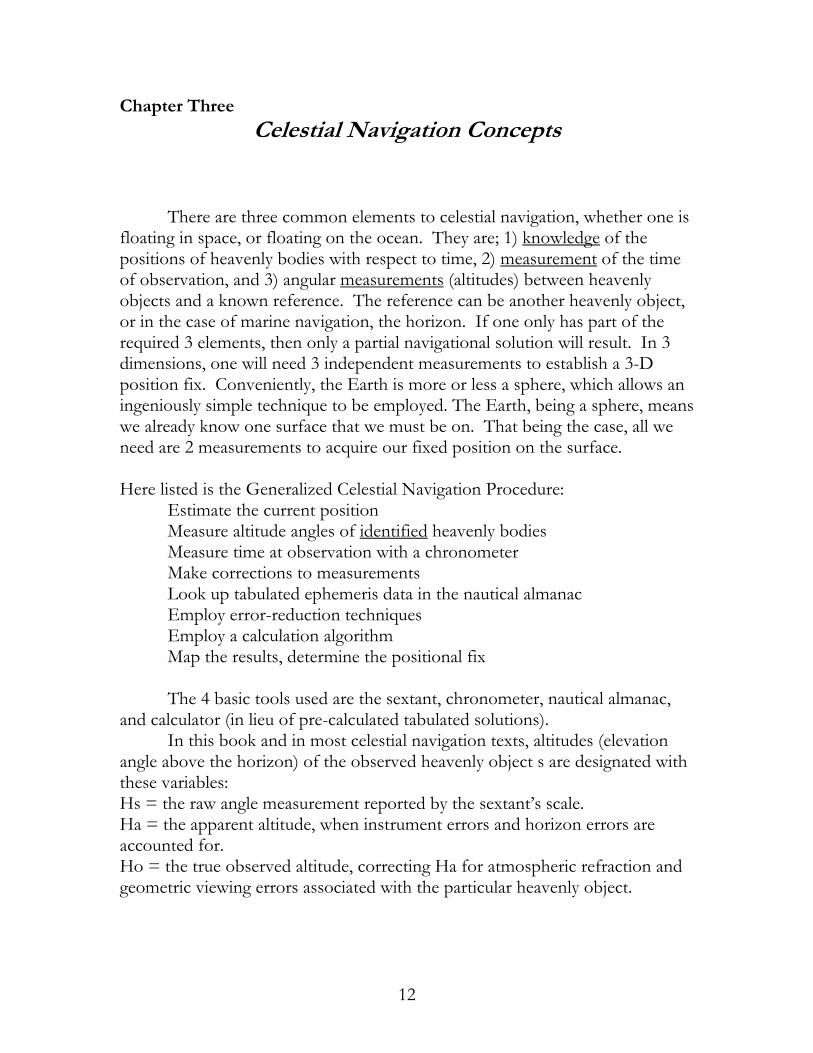
Celestial Navigation Concepts There are three common elements to celestial navigation, whether one is floating in space, or floating on the ocean. They are; 1) knowledge of the positions of heavenly bodies with respect to time, 2) measurement of the time of observation, and 3) angular measurements (altitudes) between heavenly objects and a known reference. The reference can be another heavenly object, or in the case of marine navigation, the horizon. If one only has part of the required 3 elements, then only a partial navigational solution will result. In 3 dimensions, one will need 3 independent measurements to establish a 3-D position fix. Conveniently, the Earth is more or less a sphere, which allows an ingeniously simple technique to be employed. The Earth, being a sphere, means we already know one surface that we must be on. That being the case, all we need are 2 measurements to acquire our fixed position on the surface. Here listed is the Generalized Celestial Navigation Procedure: Estimate the current position Measure altitude angles of identified heavenly bodies Measure time at observation with a chronometer Make corrections to measurements Look up tabulated ephemeris data in the nautical almanac Employ error-reduction techniques Employ a calculation algorithm Map the results, determine the positional fix The 4 basic tools used are the sextant, chronometer, nautical almanac, and calculator (in lieu of pre-calculated tabulated solutions). In this book and in most celestial navigation texts, altitudes (elevation angle above the horizon) of the observed heavenly object s are designated with these variables: Hs = the raw angle measurement reported by the sextant’s scale. Ha = the apparent altitude, when instrument errors and horizon errors are accounted for. Ho = the true observed altitude, correcting Ha for atmospheric refraction and geometric viewing errors associated with the particular heavenly object.

12

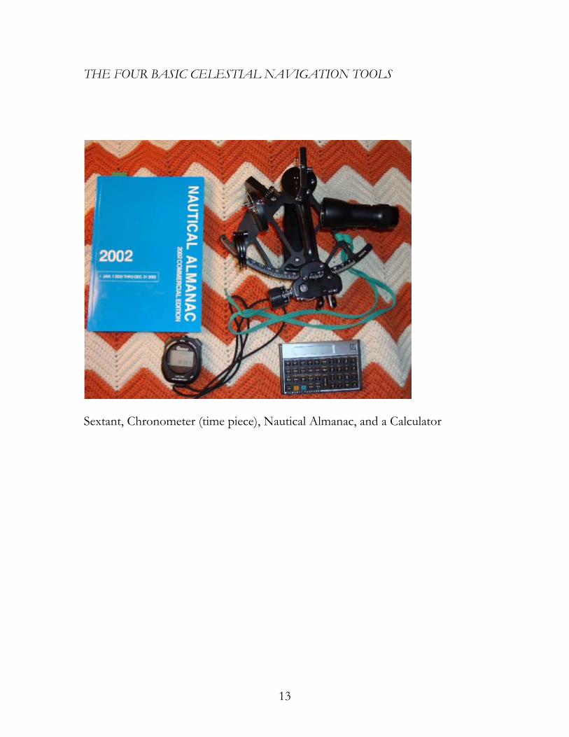
THE FOUR BASIC CELESTIAL NAVIGATION TOOLS

Sextant, Chronometer (time piece), Nautical Almanac, and a Calculator

13

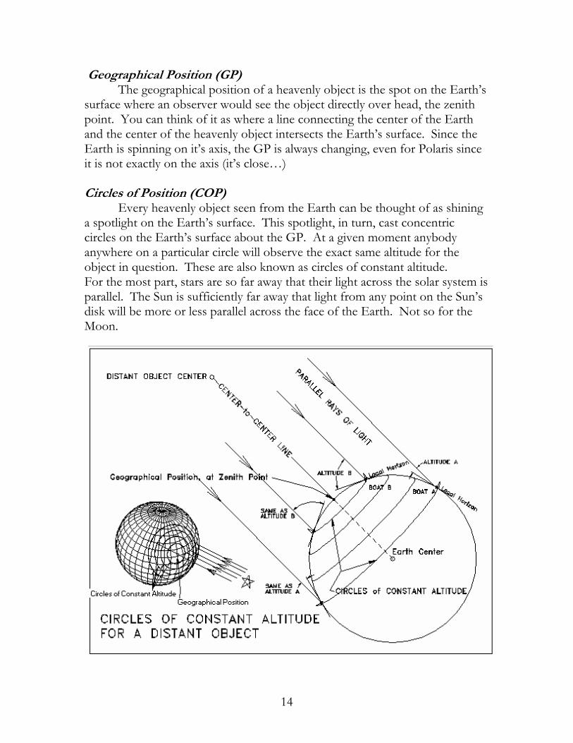
Geographical Position (GP) The geographical position of a heavenly object is the spot on the Earth’s surface where an observer would see the object directly over head, the zenith point. You can think of it as where a line connecting the center of the Earth and the center of the heavenly object intersects the Earth’s surface. Since the Earth is spinning on it’s axis, the GP is always changing, even for Polaris since it is not exactly on the axis (it’s close…) Circles of Position (COP) Every heavenly object seen from the Earth can be thought of as shining a spotlight on the Earth’s surface. This spotlight, in turn, cast concentric circles on the Earth’s surface about the GP. At a given moment anybody anywhere on a particular circle will observe the exact same altitude for the object in question. These are also known as circles of constant altitude. For the most part, stars are so far away that their light across the solar system is parallel. The Sun is sufficiently far away that light from any point on the Sun’s disk will be more or less parallel across the face of the Earth. Not so for the Moon.

14

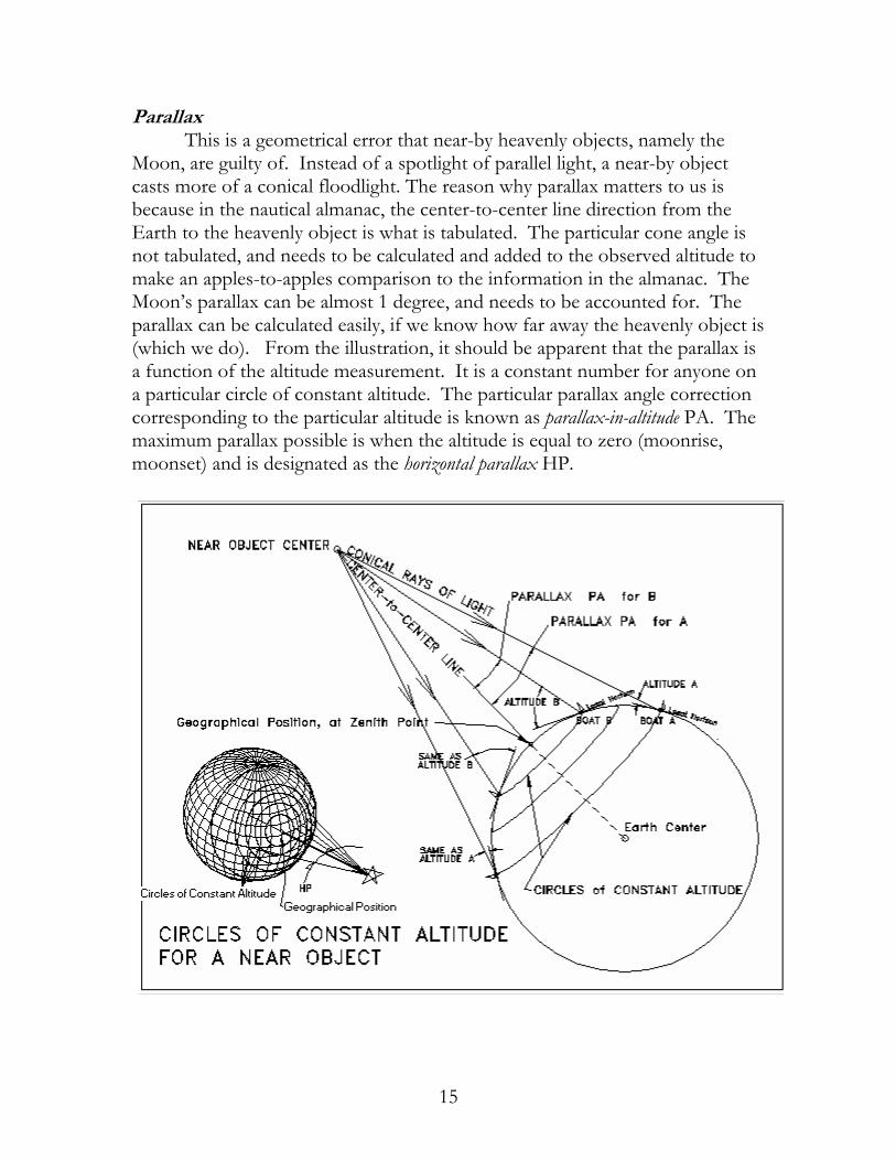
Parallax This is a geometrical error that near-by heavenly objects, namely the Moon, are guilty of. Instead of a spotlight of parallel light, a near-by object casts more of a conical floodlight. The reason why parallax matters to us is because in the nautical almanac, the center-to-center line direction from the Earth to the heavenly object is what is tabulated. The particular cone angle is not tabulated, and needs to be calculated and added to the observed altitude to make an apples-to-apples comparison to the information in the almanac. The Moon’s parallax can be almost 1 degree, and needs to be accounted for. The parallax can be calculated easily, if we know how far away the heavenly object is (which we do). From the illustration, it should be apparent that the parallax is a function of the altitude measurement. It is a constant number for anyone on a particular circle of constant altitude. The particular parallax angle correction corresponding to the particular altitude is known as parallax-in-altitude PA. The maximum parallax possible is when the altitude is equal to zero (moonrise, moonset) and is designated as the horizontal parallax HP.

15

Line of Position (LOP) Circles of Position can have radii thousands of miles across, and in the small vicinity of our estimated location on the map, the arc looks like a line, and so we draw it as a line tangent to the circle of constant altitude. This line is necessarily perpendicular to the azimuth direction of the heavenly object. One could be anywhere (within reason) on that line and measure the same altitude to the heavenly object.

16

Navigational Fix To obtain a ‘fix’, a unique latitude and longitude location, we will need two heavenly objects to observe. Reducing the measurements to 2 LOPs, the spot where it crosses the 1st line of position is our pin-point location on the map, the navigational fix. This is assuming you are stationary for both observations. If you are underway and moving between observations, then the first observation will require a ‘running fix’ correction. See the illustration of the navigational fix to see the two possibilities with overlapping circles of constant altitude. The circles intersect in two places, and the only way to be on both circles at the same time is to be on one of the two intersections. Since we know the azimuth directions of the observations, the one true location becomes obvious. Measurement errors of angle and time put a box of uncertainty around that pinpoint location, and is called the error box. We could of course measure the same heavenly object twice, but at different times of the day to achieve the same end. This will produce two different circles of constant altitude, and where they intersect is the fix, providing you stay put. If you’re not, then running fix corrections can be applied here as well. In fact, this is how navigating with the Sun is done while underway with observations in the morning, noon, and afternoon. More often than not, to obtain a reliable fix, the navigator will be using 6 or more heavenly objects in order to minimize errors. Stars or planets can be mistakenly identified, and if the navigator only has 2 heavenly objects and one is a mistake, he/she may find themselves in the middle of New Jersey instead of the middle of the Atlantic. It is improbable that the navigator will misidentify the Sun or Moon (one would hope…), but measurement errors still need to be minimized. The two measurements of time and altitude contain random errors and systematic errors. One can also have calculation errors and misidentification errors, correction errors, not to mention that you can simply read the wrong numbers from the almanac. The random errors in measurement are minimized by taking multiple ‘shots’ of the same object (~3) at approximately one minute intervals, and averaging the results in the hope that the random errors will have averaged out to zero. Systematic errors (constant value errors that are there all the time) such as a misaligned sextant, clocks that have drifted off the true time, or atmospheric optical effects different from ‘normal’ viewing conditions all need to be minimized with proper technique and attention to details, which will be discussed later. Another source of systematic error is your own ‘personal error’, your consistent mistaken technique. Perhaps you are always reading a smaller angle, or you are always 1 second slow in the clock reading. This will require a ‘personal correction’.

17

18

Surfaces of Position (SOP) If you were floating in space, you could measure the angle between the Sun and a known star. There will exist a conical surface with the apex in the Sun’s center with the axis of the cone pointing in the star’s direction whereby any observer on that conical surface will measure the exact same angle. This is a Surface of Position, where this one measurement tells you only that you are somewhere on the surface of this imaginary cone. Make another measurement to a second star, and you get a second cone, which intersects the first one along two lines. Now, the only way to be on both cones at the same time is to be on either of those 2 intersection lines. Make a third measurement between the Sun and a planet, and you will create a football shaped Surface of Position, with the ends of the football centered on the Sun and the planet. This third SOP intersects one of the two lines at one point. That is your position in 3-D.

Notice that if the football shape enlarges to infinity, the end points locally resemble cones. This is what star cones 1&2 actually are.

19

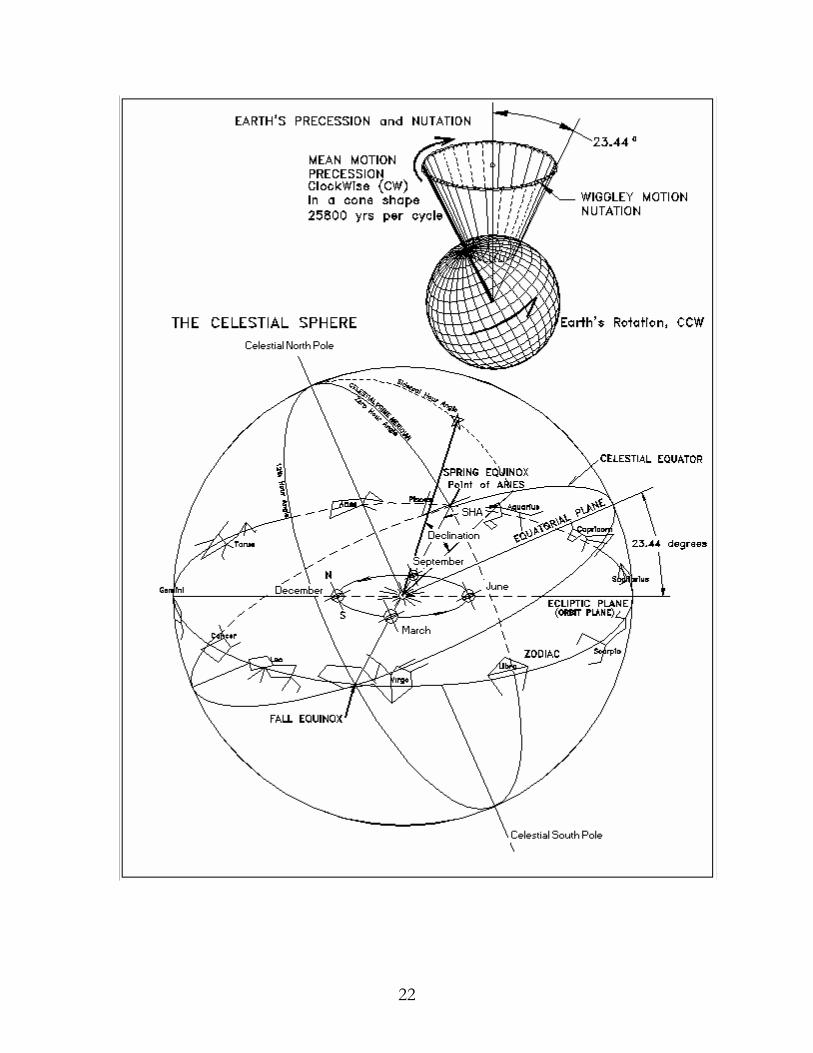
Celestial Sphere The celestial sphere is our star map. It is not a physical sphere like the Earth’s surface. It is a construction of convenience. The stars do have a 3-dimensional location in space, but for the purposes of navigation we mostly need to know only their direction in the sky. For stars, their distance is so great that their dim light across the solar system is more or less parallel. With that thought, we can construct a transparent sphere which is like a giant bubble centered over the Earth’s center where the fixed stars are mapped, painting the stars, Sun and our solar system planets on the inside of this sphere like a planetarium. We are on the inside of the bubble looking out. The celestial sphere has an equatorial plane and poles just like the Earth. In fact, we define the celestial poles to be an extension of Earth’s poles, and the two equatorial planes are virtually the same. It just does not spin. It is fixed in space while the Earth rotates inside it. In our lifetimes, the stars are more or less fixed in inertial space. However, the apparent location of a star changes slightly on the star map due to precession and nutation of the Earth’s axis, as well as annual aberration. That is, the Earth’s spin axis does not constantly point in the same direction. We usually think of the North Pole axis always pointing at Polaris, the north star. It actually wiggles (nutates) around it now, but in 10000 years it will point and wiggle about Deneb. However, 5000 years ago it pointed at Thuban and was used by the ancient Egyptians as the pole star! The Earth wobbles (precesses) in a cone-like shape just like a spinning top, cycling once every 25800 years. We know the cone angle to be the same as the 23.44 degree tilt angle of the Earth’s axis, but even that tilt angle wiggles (nutates) up and down about 9 arcseconds. There are two periods of nutation, the quickest equal to ½ year due to the Sun’s influence, and the slowest (but largest) lasting 18.61 years due to the Moon’s precessing (wobbling) orbital plane tugging on the earth. Aberration is the optical tilting of a star’s apparent position due to the relative velocity of the earth vs. the speed of light. Think of light as a stream of particles like rain (photons) speeding along at 299,792 kilometers/s. The Earth is traveling at a mean orbital velocity of 29.77 kilometers/s. When you run in the rain, the direction of the rain seems to tilt forward. The same with light. This effect can be as great as 20.5 arcseconds (3600 x arcTan(29.77/299792)). The ecliptic plane (Earth’s orbital plane at a given reference date, or epoch) mapped onto the celestial sphere is where you will also see the constellations of the zodiac mapped. These are the constellations that we see planets traverse across in the night sky, and therefore got special attention from the ancients.

20

Instead of describing the location of a star on the celestial sphere map with longitude and latitude, it is referred to as Sidereal Hour Angle (SHA) and declination (DEC) respectively. Sidereal Hour Angle is a celestial version of west longitude, and declination is a celestial version of latitude. But this map needs a reference, a zero point where its celestial prime meridian and celestial equator intersect. That point just happens to be where the Sun is located on the celestial sphere during the spring (vernal) equinox, and is known as the Point of Aries. It is the point of intersection between the mean equatorial plane and the ecliptic plane. Since the Earth’s axis wiggles and wobbles, a reference mean location for the equatorial plane is used. Due to precession of the Earth’s axis, that point is now in the zodiacal constellation of Pisces, but we say Aries for nostalgia. That point will travel westward to the right towards Aquarius thru the zodiac an average of 50.3 arcseconds per year due to the 25800 year precession cycle. Fortunately, all of these slight variations are accounted for in the tables of the nautical and astronomical almanacs. Local Celestial Sphere This is the celestial sphere as referenced by a local observer at the center with the true horizon as the equator. Zenith is straight up, nadir is straight down. The local meridian circle runs from north to zenith to south. The prime vertical circle runs from east to zenith to west.

Local celestial sphere for a ground observer

21

22

Greenwich Hour Angle GHA The Greenwich Hour Angle (GHA) of a heavenly object, is the west longitude of that object at a given instant in time relative to the Earth’s prime meridian. The Sun’s GHA is nominally zero at noon over Greenwich, but due to the slight eccentricity of Earth’s orbit (mean vs. true sun), it can vary up to 4 degrees. GHA can refer to any heavenly object that you are using for navigation, including the position of the celestial prime meridian, the point of Aries. Bird’s-eye view above the North Pole

Greenwich Hour Angle of Aries GHA (or GHAγ ) Aries

The point of Aries is essentially the zero longitude and latitude of the celestial sphere where the stars are mapped. The sun, moon, and planets move across this map continuously during the year. SHA and declination relate the position of a star in the star map, and GHAAries relates the star map to the Earth map. GHAAries is the position of the zero longitude of the star map, relative to Greenwich zero longitude, which varies continuously with time because of Earth’s rotation. The relationship for a star is thus: GHA = GHAAries + SHA = the Greenwich hour angle of a star. The declination (celestial latitude) of the star needs no ‘translation’ as it remains the same in the Earth map as in the star map. Bird’s-eye view above the north pole

23

Local Hour Angle LHA The Local Hour Angle (LHA) is the west longitude position of a heavenly object relative to a local observer’s longitude, not relative to Greenwich. This leads to the relationship: LHA = GHA + East Longitude Observer, or LHA = GHA - West Longitude Observer If the calculated value of LHA > 360, then LHA = LHACALCULATED - 360 Bird’s-eye view above the North Pole

When we are speaking of the Sun, a pre-meridian passage (negative LHA or 180<LHA < 360) means that it is still morning. A post-meridian passage (positive LHA, or 0<LHA<180) means that it is literally after noon. At exact local noon, LHA = 0

Declination DEC As stated earlier, the declination of an object is the celestial version of latitude measured on the celestial sphere star-map. Due to the tilt of the Earth’s axis of 23.44 degrees, the sun and planets change their declinations on the celestial sphere continuously during the year. The stars do not. The Sun’s declination follows nearly a perfect sine wave where over the course of 365.25 days it varies northwards 23.44 degrees and southwards –23.44 degrees. This is a crucial piece of information for the determination of latitude using the Sun.

24

As one can see, maximum declination occurs with the summer solstice which has the longest hours of daily sun, the minimum declination with the winter solstice having the shortest hours of sun, and the spring and fall equinox (“equal night”) having equal day and night times corresponding to zero solar declination. During the equinoxes, the sun will rise directly from the east and set directly in the west. At 40 degrees latitude, there are 6 more hours of daylight in the summer as compared to the winter.

Solar declination as seen by an observer on the ground varying seasonally Sign Convention We should digress momentarily to establish the proper signs for numbers, which make the mathematics consistent and unambiguous. For Declination: North is positive (+) South is negative (-) For Latitude: North is positive (+) South is negative (-) For Longitude: East is positive (+) West is negative (-) For GHA, it is a positive number between 0 and 360 degrees westward For LHA, it is positive westwards (post meridian passage) 0 <LHA < 180, and negative eastwards (pre meridian passage) -180 <LHA < 0, or 180 <LHA < 360 For observed altitude, Ho, above the horizon is positive (+)

25

Concepts in Latitude The simplest example to illustrate how latitude is determined is to consider Polaris, the North Star. Now Polaris is not exactly on the north celestial pole, but close enough for our intuition to work here. If we were sitting on Earth’s north pole (avoiding polar bears), we would observe that Polaris would be directly overhead, at the zenith point. Relative to the horizon, it would have an altitude of approximately 90 degrees of angle. Our latitude at the North Pole coincidentally is also 90 degrees. If now instead we were sweating somewhere on the equator on a hill in Ecuador at night, we would see Polaris just on the northern horizon. The altitude relative to the horizon would be approximately zero. Coincidentally, the latitude on the equator is zero. To see why this is not really a coincidence, see the illustration to understand the geometry involved. We could say generally that the observed altitude of Polaris is equal to the latitude of the observer (actually small corrections need to be made since Polaris is slightly off center from the pole). Also note that the declination of Polaris in the celestial sphere is about 90 degrees. We can generalize the matter by taking into account the declination of any particular star, as shown in the illustration. Such a star can be the Sun, and if we know the declination for every hour of the year, we can wait until the Sun is at its meridian passage (local apparent noon LAN) to make an altitude measurement Ho. The Latitude is then 90 + DEC - Ho. For a star that passes right overhead at the zenith, the star’s declination is equal to your latitude. That makes for good emergency navigation.

26

Concepts in Longitude If we think of a car traveling at 60 mph, in 2 hours it will have traveled 120 miles (60 x 2). To determine distance, all we needed was knowledge of the speed, and a clock. For a rotating object, it is the same. If we know the rotational speed, say ¼ revolutions per minute (RPM), and we have a stopwatch, in 2 minutes it should have rotated ½ revolution(0.25 x 2), or 180 degrees(0.25 x 2 x 360 degrees per rev). Now let’s think of the Earth. It rotates once in 24 hours with respect to the position of the mean Sun in the sky. That’s 360 degrees in 24 hours, or 15 degrees per hour (360/24). If a person on the Earth observes the Sun passing across the local N-S meridian line (in other words, local noon), and observes the time to be 15:00 UT, that’s 3 hours past noon in Greenwich. You will recall, UT is based on the time in Greenwich, zero longitude. The difference in angle between the observer and Greenwich, is 15 deg/hour x 3 hours = 45 degrees of longitude in the westward direction. This is why the chronometer needs to be synchronized with Greenwich time, so the observer can determine the difference in angle (longitude) with respect to the prime meridian (zero longitude). This idea was noted as early as 1530 by the Flemish professor Gemma Frisius. Pendulum clocks were not suitable for the motion of ships, and it was John Harrison in 1735 that made the first semi portable clock, with its ‘grasshopper’ escapement and twin balance-arm oscillator. A real cluge of a clock, but it was the start of marine chronometers that could take the rocking and rolling of a ship and not lose a beat. It is no coincidence that along a great arc on the Earth (such as the equator), one minute of arc (1/60 degree) corresponds to one nautical mile (n mi) of distance. One nautical mile is equal to 1.15 statute miles. The Earth’s circumference is then equal to 21600 n mi (1nm per arcmin x 60 arcmin per deg x 360 deg per full circle). The maximum surface speed of rotation for Sun observations will occur along the equator at 15 n mi per minute of time (21600 n mi per day/(24hr per day x 60 min per hr)). This is also equivalent to ¼ n mi per second of time. It is easy to see now how a time error (either the clock is off or the time is read wrong) can put the longitude determination way off. In mid latitudes, a time error of 60 seconds will put the longitude off by 10 n mi. You get the general picture, but actually the true position of the Sun does not correspond with clock time as we have already described earlier. It is a little off due to Earth’s elliptical orbit. The upshot of all this explanation is that to know longitude, one needs to have a clock set to the time in Greenwich England.

27

Noon Sighting The noon sighting is an old way of determining latitude and (with misgivings) longitude, as the azimuth is unambiguously known as either due south or due north. The method is more educational than accurate. Here, the trigonometry disappears and reduces down to mere arithmetic. The technique is to predict approximate local apparent noon (LAN) for your estimated longitude from dead reckoning navigation. Take sightings with your sextant several minutes before LAN, and with a sighting every minute, capture the highest point in the sky that the Sun traveled plus some sightings after meridian passage. You make corrections to obtain the true altitudes, and plot this information as true altitude versus time. From the plot you can smooth the curve and determine the highest point (Honoon) and estimate the time of LAN to within several minutes or better of Universal Time (~20 n miles of longitude error). Using the nautical almanac, obtain the GHA and declination of the Sun (DEC) at the time of LAN. Remember the sign convention and apply it. We will now make a distinction regarding the direction of meridian passage, whether the sun peaked in the south or in the north, by introducing a new variable Signnoon. In keeping with the consistent sign convention, when the meridian passage is northwards such as commonly occurs in S. latitudes, the value of Signnoon is +1. When the meridian passage is southwards such as commonly occurs in N. latitudes, the value of Signnoon is -1. Thus: Latitude = Signnoon x Honoon + DEC + 90 If this calculated latitude is greater than 90 degrees, then subtract 180 from it. If Signnoon x Honoon + DEC is equal to zero, then you are exactly on either the north or south pole. If you don’t know which pole you’re on then you should have stayed home. This equation works whether you are in the northern or southern hemispheres, in or out of the tropics. Just follow the sign convention, and it will all come out fine. For longitude, the local hour angle LHA is zero, and so: Longitude = - GHA if GHA is less than 180 Longitude = 360 – GHA if GHA is greater than 180 Remember, if your chronometer is inaccurate then the longitude will be off considerably since you are in essence comparing the local time with time in Greenwich. It will be off considerably anyway due to the plotting estimates.

28

Plane Trigonometry The simplest notion of ‘trig’ is the relationship of the sides and angles in a triangle. All you have to know are these three basic relationships:

sine (α) = Lo / H shorthand is sin(α) cosine (α) = La / H shorthand is cos(α) tangent (α) = Lo / La shorthand is tan(α) The values of these trigonometric functions can be expressed as an infinite series, which your calculator will approximate by truncating the series after evaluating only a few terms.

Useful identities: sin(α) = cos(α -90˚) cos(α) = - sin(α -90˚) Spherical Trigonometry

Three Great Circles on a sphere will intersect to form three solid corner angles a, b, c, and three surface angles A, B, C. Every intersecting pair of Great Circles is the same as having two intersecting planes. The angles between the intersecting planes are the same as the surface angles on the surface of the sphere. Relationships between the corner angles and surface angles have been worked out over the centuries, with the law of sines and the law of cosines being the most relevant to navigation.

Law of Sines: sin(a)/sin(A) = sin(b)/sin(B) = sin(c)/sin(C) Law of Cosines: cos(a) = cos(b) • cos(c) + sin(b) • sin(c) • cos(A)

29

The Navigational Triangle The navigational triangle applies spherical trigonometry, in that the corner angles a, b, c are related to altitude, latitude, and declination angles, and the surface angles are related to azimuth and LHA angles.

The corner angles corresponding to the arc sides are modifications of the altitude, latitude and declinations. As can be seen in the drawing, they are 90˚ –the angle, known as co-angles: Co-altitude = 90˚ – H Co-declination = 90˚ – DEC Co-latitude = 90˚ - LAT Most authorities will examine 4 cases concerning North or South declination and latitude. But if a consistent sign convention is used, we need only concern ourselves with the one picture.

30

Chapter Four

Calculations for Line of Position The calculated altitude is a way of predicting the altitude of a heavenly object by first assuming a latitude and longitude for a hypothetical observer and working out the problem backwards. The math becomes direct and unambiguous when done in this manner. The obvious choice of assumed latitude and longitude is the estimated position by dead reckoning. Dead reckoning is the method of advancing from a last known position by knowing the direction you headed in, how fast you were going, and how long you went. You will eventually compare this calculated altitude to a measured altitude, and so the calculated altitude must correspond to the same time as the measured altitude. This is important to extract the proper values of GHA and declination from the nautical almanac. You must be talking about the same instant in time for a correct comparison. Remembering to use the sign convention, the law of cosines gives us this relationship for the calculated altitude Hc: Hc = arcSin[ Sin(DEC) • Sin(LatA) + Cos(LatA) • Cos(DEC) • Cos(LHA) ] Where LatA is the assumed latitude, LonA is the assumed longitude and the calculated local hour angle LHA = GHA + LonA If LHA is greater than 360, then subtract 360 from the calculated LHA. DEC is of course the declination of the heavenly object. The uncorrected azimuth angle Zo of a heavenly object can also be calculated as thus: Zo = arcCos[{Sin(DEC) – Sin(LatA) • Sin(Hc)}/{Cos(LatA) • Cos(Hc)}] Corrected azimuth angle Z (not used in any of the equations here) If N. latitudes, then Z = Zo If S. latitudes, then Z = 180 – Zo True Azimuth Angle from True North Zn If LHA is pre-meridian passage (-, or 180<LHA < 360), Zn = Zo If LHA is post-meridian passage (0<LHA < 180), Zn = 360 – Zo Post meridian check can also be established if: Sin(LHA) > 0

31

By using the sign convention, we only have two cases to examine to obtain the true azimuth angle. All texts on celestial that I know of will list 4 cases due to the inconsistently applied signs on declination and latitude. Classical same name (N-N, S-S) or opposite name (N-S, S-N) rules do not apply here. Line of Position by the Marcq Saint-Hilaire Intercept Method This clever technique determines the true line of position from an assumed line of position. Let’s say you measured the altitude of the Sun at a given moment in time. You look up the GHA and declination of the Sun in the nautical almanac corresponding to the time of your altitude measurement. From an assumed position of latitude and longitude, you calculate the altitude and azimuth of the Sun according to the preceding section and arrive at Hc and Zn. On your map, you draw a line thru the pin-point assumed latitude and longitude, angled perpendicular to the azimuth angle. This is your assumed line of position. The true line of position will be offset from this line either towards the sun or away from it after comparing it to the actual observed altitude Ho (the raw sextant measurement is Hs, and needs all the appropriate corrections applied to make it an ‘observed altitude’). The offset distance DOFFSET to determine the true line of position is equal to: DOFFSET = 60 • (Ho - Hc), altitudes Ho and Hc in decimal degrees, or DOFFSET = (Ho - Hc), altitudes in minutes of arc. DOFFSET in nautical miles for both cases. If DOFFSET is positive, then parallel offset your assumed line of position in the azimuth direction towards the heavenly object. If negative, then draw it away from the heavenly object. If the offset is greater than 25 nautical miles, you may want to assume a different longitude and latitude to minimize errors. By calculating an altitude, you have created one circle of constant altitude about the geographical position, knowing that the actual circle of constant altitude is concentric to the calculated one. The difference in observed altitude and calculated altitude informs you how much smaller or larger the actual circle is. Offsetting along the radial azimuth line, the true circle will cross the azimuth line at the intercept point.

32

33

Line of Position by the Sumner Line Method If we measure the altitude of a heavenly object and make all the proper corrections, this reduces to the observed altitude Ho. As we should know by now, there is a circle surrounding the geographical position of the heavenly object where all observed altitudes have the same value Ho. We could practically draw the entire circle on the map, but why bother? What if instead, we draw a small arc in the vicinity of our dead reckoning position. In fact, why an arc at all, since at the map scale that interest us, a straight line will do just fine. All we need do is to rearrange the equation of calculated altitude, to make it the observed altitude instead and to solve the equation for LHA, which will give us longitude. The procedure is to input an assumed latitude, the GHA and declination for the time of observation, and out pops a longitude. Mark longitude and latitude on the map. Now input a slightly different latitude, and out pops a slightly different longitude. Mark the map, connect the dots and you have a Sumner Line. These are two points on the circle in the vicinity of your dead reckoning position. Or were they? Was the answer for longitude unreasonably off? Notice that for every latitude line that crosses the circle, there are 2 solutions for longitude, an east and west solution. In the arcCos function, the answer can be the angle A or the angle -A. Check both just to make sure. East side of the circle when the object is westwards (post meridian): LonC = arcCos[{ Sin(Ho) - Sin(DEC) • Sin(LatA)}/{Cos(LatA) • Cos(DEC)}] – GHA West side of the circle when the object is eastwards (pre meridian): LonC = -arcCos[{ Sin(Ho) - Sin(DEC) • Sin(LatA)}/{Cos(LatA) • Cos(DEC)}] – GHA Where LatA is the assumed latitude, LonC is the calculated longitude DEC is of course the declination of the heavenly object. The two values for assumed latitude could be the dead reckoning latitude LatDR

+ 0.1 and – 0.1 degree. The advantage to this method is that the LOP comes out directly without offsets. There is no azimuth calculation, just two calculations with the same equation having slightly differing latitude arguments. Also, the fact that only the assumed latitude is required means no estimated position of the longitude is needed at all. This method turns into an E-W LOP when near the meridian passage. It’s as if you were doing a ‘noon shot’ when under these circumstances, so just use the DR latitude and draw an E-W line.

34

35

History of the Sumner Line The Sumner line of position takes its name from Capt. Thomas H. Sumner, an American ship-master, who discovered the technique serendipitously and published it. This is the incident as described in his book, which lead to its discovery: Having sailed from Charleston, S. C., November 25th, 1837, bound for Greenock, a series of heavy gales from the westward promised a quick passage; after passing the Azors the wind prevailed from the southward, with thick weather; after passing longitude 21 W. no observation was had until near the land, but soundings were had not far, as was supposed from the bank. The weather was now more boisterous and very thick, and the wind still southerly; arriving about midnight, December 17th within 40 miles, by dead reckoning, of Tuskar light, the wind hauled SE. true, making the Irish coast a lee shore; the ship was then kept close to the wind and several tacks made to preserve her position as nearly as possible until daylight, when, nothing being in sight, she was kept on ENE. under short sail with heavy gales. At about 10 a. m. an altitude of the sun was observed and the chronometer time noted; but, having run so far without observation, it was plain the latitude by dead reckoning was liable to error and could not be entirely relied upon. The longitude by chronometer was determined, using this uncertain latitude, and it was found to be 15' E. of the position by dead reckoning; a second latitude was then assumed 10' north of that by dead reckoning, and toward the danger, giving a position 27 miles ENE. of the former position; a third latitude was assumed 10' farther north, and still toward the danger, giving a third position ENE. of the second 27 miles. Upon plotting these three positions on the chart, they were seen to be in a straight line, and this line passed through Smalls light. It then at once appeared that the observed altitude must have happened at all of the three points and at Smalls light and at the ship at the same instant.

Then followed the conclusion that, although the absolute position of the ship was uncertain, she must be somewhere on that line. The ship was kept on the course ENE. and in less than an hour Smalls light was made, bearing ENE. 1/2E. and close aboard.

36

Chapter 5 Measuring Altitude with the Sextant The sextant is a wonderfully clever precision optical instrument. It reflects the image of the Sun (or anything, really) twice with two flat mirrors in order to combine it with a straight-thru view, allowing you to see the horizon and heavenly object simultaneously in the same pupil image. This allows for a ‘shake-free’ view, as the horizon and Sun move together in the combined image. The straight-thru view is accomplished with the second mirror (horizon mirror), which is really a half mirror, silvered on the right and clear on the left. You see the horizon unchanged on the left, and the twice-reflected sun on the right if you use a ‘traditional’ mirror as opposed to a ‘whole horizon’ mirror. With a whole horizon mirror, both horizon and Sun will be in the entire view. It does this by partial silvering of the entire horizon mirror like some sunglasses are, reflecting some light and transmitting the rest. This makes the easy shots easier, but the more difficult shots with poor illumination or star shots more difficult. Even with the traditional mirror, curiously, you will see a whole image of the sun in the pupil that you can move to the right or left by rocking the sextant side to side. The glass surface itself is reflective. When it is at its lowest point, you are correctly holding the sextant and can take a reading. The horizon however, will only be on the left side of the image. In order to determine the altitude of the Sun, you change the angle of the first mirror (index mirror) with the index arm until the Sun is close to the horizon in the pupil image. Now turn the precision index drum (knob) until the lower limb of the Sun just kisses the horizon. Rock it back and forth to make sure you have the lowest reading. In order not to burn your eye out (that would be stupid…), there are filters (shades) that can be rotated over the image path of the index mirror. Likewise, there are other filters that cover the horizon mirror to remove the glare and increase the contrast between horizon and sky.

37

38

Mirror Alignments Even an expensive precision instrument will give you large errors (although consistent systematic error) unless it is adjusted and calibrated. Before any round of measurements are taken, you should get into the habit of calibrating and if necessary adjusting the mirrors to minimize the errors. The first check is to see if the index mirror is perpendicular to the sextant’s arc. Known as Perpendicularity Alignment, it is checked in a round-about manner by finding the image of the arc in the index mirror when viewed externally at a low angle. Set the arc to about 45 degrees. The reflected arc in the index mirror should be in line with the actual arc. This can be tricky, as it only works if the mirrored surface is exactly along the pivot axis of the index arm. Since most mirrors are secondary surface mirrors (the silvering is on the back of the glass), you need to compare the position of the rear of the glass to the pivot axis first to see if this technique will work. First surface mirrors (the silvering is on the front of the glass) seem to be an upgrade, but the sextant’s manufacturer may not have necessarily redesigned the mirror-holding mount. This positions the index mirror reflecting surface 2 to 3 mm or so in front of the pivot axis. In that case, the reflected image of the arc should be slightly below the viewed actual arc. There are precision-machined cylinders about an inch high that you can place on the arc and view their reflections. The reflections should be parallel to the actual cylinders. If not, then turn the set screw behind the index mirror to bring it into perpendicular alignment. The next alignment is Side Error Alignment of the horizon mirror. This can be done two ways after setting the arc to the zero angle point such that you see the same object on the left and right in the pupil image. First, at sea in the daytime, point the sextant at the horizon. You will see the horizon on the left and the reflected horizon on the right. Adjust the index drum until they are in perfect alignment while holding the sextant upright. Now roll (tilt) the sextant side to side. Is the horizon and reflected image still line-to-line? If not, then side error exists. This is corrected with adjustments to the set screw that is perpendicularly away from the plane of the arc on the horizon mirror. Second method is to wait until nighttime, where a point source that is nearly infinitely far away presents itself (yes, I mean a star). Same procedure as before except that you need not roll the sextant. What you will see is two points of light. The horizontal separation is the side error, and the vertical separation is the index error. Adjust the drum knob to negate the index error effect until the star and its reflection are vertically line-to-line but still separated horizontally. Make adjustments to the side-error set screw until the points of light converge to a single image point.

39

You could stop here at this point, reading the drum to determine the index error IE (Note: index correction IC = - IE). Or you could continue to zero out the index error as well with a last series of adjustments. In which case, for the Index Error Alignment, set the arc to zero (index arm and drum to the zero angle position). You will notice that the star image now has two points separated vertically. Adjusting the remaining set screw on the horizon mirror (which is near the top of the mirror), you can eliminate the vertical separation. Unfortunately this last set screw does not only change the vertical separation, but it slightly affects the horizontal separation as well. Now you need to play around with both set screws until you zero-in the two images simultaneously. With a little practice these procedures will be easy and routine. A word of caution: the little wrench used to adjust the set screws maybe very difficult to replace if you should drop it overboard. Making a little hand lanyard for the wrench will preserve it. Maybe… Note: I have also used high altitude jet aircraft, their contrails, and even cloud edges to adjust the mirrors. If you have dark enough horizon shades, you can even use the sun’s disk to adjust the mirrors.

40

Sighting Techniques Bringing the object down Finding the horizon is much easier than finding the correct heavenly object in the finder scope. So, the best technique is to first set the index arm to zero degrees and sight the object by pointing straight at it. Then keeping it in view, ‘lower’ it down to the horizon by increasing the angle on the index arm until the horizon is in sight. Careful with the sun, as you don’t want to see it unfiltered thru the horizon glass; keep the sun on the right hand side of the mirror using the darkest shade over the index mirror. Rocking for the lowest position Rocking the sextant from side to side will help you determine when the sextant is being pointed in the right direction and held proper, as the object will find its lowest point. This will give the true sextant altitude Hs. Letting her rise, letting her set Often it is easier to set the sextant ‘ahead’ of where the heavenly object is going, and to simply let her rise or set as the case may be to the horizon. At that point you mark the time. That way you can be rocking the sextant to get the true angle without also fiddling with the index drum. This leaves a hand free, sort of, to hold the chronometer such that at the time of mark, you just have to glance to the side a little to see the time. Upper limb, lower limb With an object such as the Sun or Moon, you can choose which limb to use, the lower limb or upper limb. Unless the Sun is partially obscured by clouds, the lower limb is generally used. Depending on the phase of the moon, either lower limb or upper limb is used.

41

Brief History of Marine Navigational Instruments The earliest instrument was the astrolabe, constructed in the Middle East during the 9th century AD. It was a mechanical rotating slide rule with a pointer to determine the altitude of stars against a protractor. Contemporary was a very simple instrument, the quadrant. It was a quarter of a circle protractor with a plumb-bob and a pair of peep sights to line up with Polaris. The first real ancestor to the modern sextant was the cross staff, described in 1342. A perpendicular sliding cross piece over a straight frame allowed one to line up two objects and determine the angle. Of course one had to look at both objects simultaneously by dithering the eyeball back and forth – a bit of a problem. Also one had to look into the blinding sun. Since a cross staff looked like a crossbow, one was said to be ‘shooting the sun’, an expression still used today. The Davis backstaff in 1594 was an ingenious device where sun shots were taken with your back to the sun, using the sun’s shadow over a vane to cast a sharp edge. The navigator would line up the horizon opposite the sun azimuth with a pair of peep holes, and rotated a shadow vane on an arc until the shadow edge lined up on the forward peep hole. This limited one to only sun shots to determine latitude. In the 1600’s a French soldier-mathematician by the name of Vernier invented the vernier scale, whereby one could easily interpolate between degree scales to a 1/10 or 1/20 between the engraved lines on the protractor scale. The search for determining longitude created bizarre proposals, but it was recognized that determining the time was the answer, and so one needed an accurate clock. A clock could be mechanical, or astronomical. The Moon is about ½ degree of arc across its face, and moves across the celestial sphere at the rate of about one lunar diameter every hour. Therefore its arc distance to another star could be used as a sort of astronomical clock. Tables to do this were first published in 1764. The calculations and corrections are indeed frightening, and this method of determining time to within several minutes of Greenwich Mean Time is called doing Lunars, and those who practice it are Lunarians. Undoubtedly if you used this method too often you would have been branded a Lunatic. Fortunately in 1735 John Harrison invented the first marine chronometer, having some wood elements and weighing 125 lbs. He worked on it for 40 years! The Hadley Octant in 1731 was the first to use the double reflecting principle as described by Isaac Newton a century before. It could measure across 90 degrees of arc, even though it was only physically 45 degrees arc, an 1/8 of a circle. The sextant with it’s ability to record angles of 120 degrees came about for use in doing lunars, and so was a contemporary of the octant. By 1780, refinements such as tangential screws, vernier scales, and shades glasses, fixed the design of sextants and octants for the next 150 years.

42

VARIOUS ANTIQUE INSTRUMENTS

43

Chapter 6 Corrections to Measurements There are numerous corrections to be made with the as-measured altitude Hs that you read off of the sextant’s arc degree scale and arc minute drum and vernier. Your zero point on the scale could be off, the same as the bathroom scale when you notice that it says you weigh 3 lbs even before you get on it. This is known as index error, and the correction is IC. For our example of the bathroom scale, IC = -3. The other major corrections are parallax, semi-diameter, refraction, and dip, listed from the largest effect to the smallest. Lunar parallax can be at most a degree, semi-diameter ¼ degree, refraction and dip are on the order of 1/20th degree.

The Hs in the figure does not account for the index error, IC.

44

The sextant basically has an index correction IC and an instrument correction I. The instrument error is due to manufacturing inaccuracies and distortions, and should be listed on a calibration sheet from the manufacturer. Generally it’s negligible. Index error is due to the angular misalignment of the index mirror, with respect to the zero point on the scale. Dip Correction Dip is the angle of the visual horizon, dipping below the true horizon due to your eye height above it. This is also tabulated in the nautical almanac. An approximate equation for dip correction that incorporates a standard horizon refraction is thus: Corr DIP = - 0.0293 • SquareRoot(h) Decimal Degrees Where h is the eye height above the water, meters. Corr DIP is always negative. Altitude Corrections Let us first define the apparent altitude, Ha = Hs + IC + Corr DIP Ha is the altitude without corrections for refraction, semi-diameter, or parallax. The atmosphere bends (refracts) light in a predictable way. These corrections are tabulated on the 1st page of the nautical almanac based on the apparent altitude Ha. The corrections vary for different seasons, and whether you are using the lower or upper limb of the Sun for your observations. Since measurements are made to the edge (limb) and not the center of the Sun, the angle of the Sun’s visual radius (semi-diameter) must be accounted for. The table also lists slight deviations from the nominal for listed planets. There are special lunar correction tables at the end of the almanac, which include the effects of lunar semi-diameter, parallax and refraction. The variable name for all of these combined altitude error corrections, lunar, solar or otherwise, is Corr ALT, sometimes called the ‘Main Correction’. The true observed altitude is a matter of adding up all the corrections: Ho = Ha + Corr ALT

45

Tables of Altitude Correction, averaged values, summer/winter

Altitude correction for sun and stars CorrALT

Ha Sun LL

Sun UL Stars

10 deg +11' -21' -5' 13

deg +12' -20' -4' 15

deg +12.5' -19.5' -3.5' 17

deg +13' -19' -3' 20

deg +13.5' -18.5' -2.5' 24

deg +14' -18' -2' 31

deg +14.5' -17.5' -1.5'

41deg +15' -17' -1' 59

deg +15.5' -16.5' -0.5' 85

deg +16' -16' 0

Dip Correction Height CorrDIP 0.7m -1.5' 1.3m -2' 2.0m -2.5' 2.9m -3' 3.9m -3.5' 5.1m -4' 6.4m -4.5'

46

Refinements Corrections for observations can be calculated instead of using tables, and refinements can be employed for non-standard conditions. Start with the apparent altitude Ha: Ha = Hs +IC + Corr DIP (assume instrument correction I ~0) The horizontal parallax for the Moon is given in the nautical almanac tables as the variable HP in minutes of arc, and you must convert it to decimal degrees. HP for the Sun = 0.0024 degrees, but this is rarely included as being so small a value. For Venus, the HP is hidden in the altitude correction tables, listed as ‘Additional Corrn ’. Use the largest number at zero altitude to = HPVenus. To determine the parallax-in-altitude PA, use this equation: PA = HP • Cos(Ha) • (1 –(Sin2(Lat))/297) includes earth oblateness The semi-diameter of the Sun SD is given at the bottom of the page of the tables in the nautical almanac in minutes of arc, and you must convert it to decimal degrees. So is the semi-diameter daily average of the Moon, but you can calculate one based on the hourly value of HP: The semi-diameter of the Moon: SD = 0.2724 • HP • (1 + Sin(Ha)/230) The terms in the parenthesis are “augmentation”, meaning the observer is a very little closer to the moon with greater altitude angle. This is a small term. Atmospheric refraction is standardized to surface conditions of 10 deg C and 1010mb pressure. This standard refraction correction Ro is thus: Ro = - 0.0167 / Tan[Ha + 7.31/(Ha+4.4)] degrees The correction for non-standard atmospheric conditions is referred to as f: f = 0.28 • Pressuremb / (TemperatureDEG C + 273) The final refraction correction R is thus: R = Ro • f This number is always negative. If the lower limb were observed, then signlimb = +1 If the upper limb were observed, then signlimb = -1 Observed altitude with refinements: Ho = Ha + R + PA + SD • signlimb Here we see that the altitude correction Corr ALT = R + PA + SD • signlimb Note: Convert arcminutes to decimal degrees for consistent calculations

47

Artificial horizon A fun way of practicing sighting the Sun while on land is to use an artificial horizon. This is simply a pan of water or old motor oil that you place down on the ground in view of the Sun. Since the liquid will be perfectly parallel with the true horizon (no dip corrections here), it can be used as a reflecting plane. In essence you point the sextant to the pan of liquid where you see the reflection of the Sun. Move the index arm until you bring the real Sun into the pupil image with the index mirror. With the micrometer drum bring both images together (no semi-diameter corrections either) and take your reading. This gives a reading nearly twice the real altitude. Undoubtedly you will need to position extra filters over the horizon mirror to darken the Sun’s image, as normally you would be looking at a horizon. Correct the reading by taking the apparent altitude Ha and divide by two, then add the refraction correction: Ha = (Hs + IC)/2 no dip correction Ho = Ha + R no semi-diameter correction The wind is very bothersome, as it will ripple the water’s surface and therefore the reflected image. Protective wind guards around the pan work somewhat, but generally you may have to wait minutes for a perfect calm. What works best is mineral oil in a protected pan set up on a tripod so that you can get right up to it. The ripples dampen out almost immediately. To be very accurate, you can let the sun touch limb-to-limb. If pre meridian (morning) then let the bottom image rise onto the reflected image, measure the time, and SUBTRACT a semidiameter (UL): Ho = Ha + R - SD If post meridian (afternoon), let the top image set onto the reflected image, measure the time, and ADD a semidiameter (LL): Ho = Ha + R + SD

48

Chapter 7 Reading the Nautical Almanac The nautical almanac has detailed explanations in the back regarding how to read the tabular data and how to use the interpolation tables (increments and corrections). The data is tabulated for each hour on the dot for every day of the year, and you must interpolate for the minutes and seconds between hours. Every left hand page in the almanac is similar to all other left hand pages, and the same for all right hand pages. Three days of data are presented for every left and right hand page pairs. The left page contains tabular data of GHA and declination for Aries (declination = 0), Venus, Mars, Jupiter, Saturn and 57 selected stars. The right page has similar data for the Sun and Moon. It also provides the Local Mean Time (LMT) for the events of sunrise, sunset, moonrise, and moonset at the prime meridian. For your particular locality, you can express the event time in UT with the following equation: EventTimeLOCAL = LMT – Longitude/15. Hours UT at your longitude. Remember the sign convention, West -, East +. Interpolation tables, v and d corrections Probably the most confusing part of the tables is interpolation for times between hourly-tabulated data, and how to properly apply the mysterious v and d corrections. The interpolation tables (‘increments and corrections’) are based on nominal rates of change of GHA for the motions of the Sun and planets, Moon, and Aries. This way, only one set of interpolation tables is required, with variances to the rates compensated with the v and d values. These are hourly variances, and their applicable fraction (the correction Corr V and Corr d) is given in the interpolation tables for the minute of the hour. The v number refers to variances in the nominal GHA rate. There is no nominal rate for changes in declination, so d is the direct hourly rate of change of declination. For GHA, the interpolation tables will tabulate increments (Corr GHA) down to the second of each minute. The v and d correction is interpolated only for every minute. Take the hourly data in the tables, GHA, add the interpolated increment for the minutes and seconds, and finally add the interpolated v correction. Similarly for declination, take the tabulated hourly value Dec and add the interpolated d correction. Our sign convention imposes that a south declination is negative, and a north declination is positive. A word of caution, the value of d (with our sign convention) may be positive or negative. If the tabulated hourly data for declination is advancing northwards (less southwards), then the sign is positive. We could have a negative declination (south), but have a positive d if declination is becoming less southwards. Along the same line, we

49

could have a positive declination (north) but a negative d if the declination is heading south (less northwards). The final values at the particular hour, minute, and second are thus: GHA = GHAhour + Corr GHA + Corr V DEC = DEC hour + Corr d Where GHAhour and DEC hour are the table values in the almanac for the hour. After all the interpolations and corrections are performed, convert the angles to decimal degrees and make sure the sign convention was applied consistently to the declination value. Note: In the nautical almanac, liberal use is made of the correction factor Corrn. It seems to appear everywhere and applied to everything. The n is actually a variable name for any of the parameters that require ‘correction’. Notably, Corr DIP, Corr ALT, Corr GHA, Corr V, and Corr d. Since we like to use our calculators, instead of using the ‘increments and corrections’ table (it’s actually very easy) we can interpolate for ourselves in the following manner. Lets say we shot an observation at Universal Time H hours, M minutes, and S seconds (H:M:S). The nautical almanac tables for the particular day gave us a GHA in degrees and arcminutes at the UT hour. We convert it to decimal degrees and call it GHAhour. We do the same for the declination and call it DEC hour. Note the hourly variance v and declination rate d in arcminutes per hour. We can also define the hour fraction, Δt, which are the minutes and seconds in decimal form: Δt = (M/60) + (S/3600). Now, the correct interpolated value for our specific time of observation is thus: GHA = GHAhour + {Rate + (v/60)} x Δt decimal degrees Where Rate = 15.00000 (degrees/hour) for Sun or planets Rate = 14.31667 (degrees/hour) for Moon Rate = 15.04107 (degrees/hour) for Aries In a similar line, declination is interpolated thus: DEC = DEC hour + (d/60) x Δt (DEC hour and d with the proper sign) Carry out all calculations to 4 decimal places, and make sure the sign convention was applied correctly (carpenter’s rule: measure twice, cut once). Visit an on-line Nautical Almanac at: http://www.tecepe.com.br/scripts/AlmanacPagesISAPI.isa

50

51

52

Chapter 8 Sight Reduction The process of taking the raw observational data and turning the information into a Line Of Position (LOP) is called sight reduction. Even though the equations and methods have been described all through out the book, what is needed here most is organization to minimize the calculation random errors. History Trigonometric tables were first published by Regiomontanus in the mid 1400's, followed by the early logarithm tables of Edmund Gunter in the late 1600’s, which allowed multiplication to be treated as addition problems. This is the basis of the slide rule (does anybody remember those??). French almanacs were published in the late 1600’s where the original zero longitude ‘rose line’ ran thru Paris. The English almanacs were published later in the 1700’s. The altitude-difference method of determining a line of position introduced the age of improved navigation, described in 1875 by Commander Adolphe-Laurent- Anatole Marcq de Blonde de Saint-Hilaire, of the French Navy. This ‘Marcq Saint-Hilaire’ method remains the basis of almost all celestial navigation used today. But the Sumner line method may be considered equally easy, 2 computations for the Saint-Hilaire method, and 2 for the Sumner line method. Computed altitude and azimuth angle have been calculated by means of the log sine, cosine, and haversine ( ½ [1-cos] ), and natural haversine tables. Sight reduction was greatly simplified early in the 1900’s by the coming of the various short-method tables - such as the Weems Line of Position Book, Dreisonstok's Hydrographic Office method H.O. 208 (1928), and Ageton's H.O. 211 (1931). Almost all calculations were eliminated when the inspection tables, H.O. 214 (1936), H.O. 229, and H.O. 249 were published, which tabulated zillions of pre-computed solutions to the navigational triangle for all combinations where LHA and latitude are whole numbers. The last two methods, H.O. 229 and H.O. 249 developed in the mid 1940’s and early 1950’s remain the principle tabular method used today. The simplest tabular method of all is to use a shorthand version of Ageton’s tables known as the S-tables, which are only 9 pages long. No whole number assumptions are required, and the answers are the same as a navigational calculator. You must do some minor addition, though. The following page is an example of a sight-reduction form using the “calculator method” instead of the typical HO 229, 249 tabular methods.

53

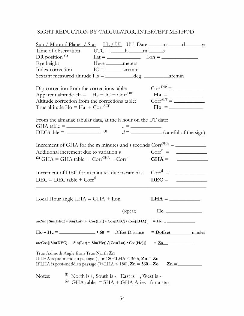
SIGHT REDUCTION BY CALCULATOR, INTERCEPT METHOD Sun / Moon / Planet / Star LL / UL UT Date _____m _____d______yr Time of observation UTC = _____h _____m _____s DR position (1) Lat = ____________ Lon = _____________ Eye height Heye ______meters Index correction IC = ______ arcmin Sextant measured altitude Hs = __________deg _________arcmin Dip correction from the corrections table: CorrDIP = ___________ Apparent altitude Ha = Hs + IC + CorrDIP Ha = ____________ Altitude correction from the corrections table: CorrALT = ___________ True altitude Ho = Ha + CorrALT Ho = ____________ From the almanac tabular data, at the h hour on the UT date: GHA table = ____________ v = ___________ DEC table = ____________ (1) d = ___________ (careful of the sign) Increment of GHA for the m minutes and s seconds CorrGHA = ___________ Additional increment due to variation v Corrv = ___________ (2) GHA = GHA table + CorrGHA + Corrv GHA = ___________ Increment of DEC for m minutes due to rate d is Corrd = ___________ DEC = DEC table + Corrd DEC = ___________ _____________________________________________________________ Local Hour angle LHA = GHA + Lon LHA = ___________ (repeat) Ho _______________ arcSin[ Sin(DEC) • Sin(Lat) + Cos(Lat) • Cos(DEC) • Cos(LHA) ] = Hc _ ______________ Ho – Hc = _______________ • 60 = Offset Distance = Doffset n.miles arcCos[{Sin(DEC) – Sin(Lat) • Sin(Hc)}/{Cos(Lat) • Cos(Hc)}] = Zo ______________ True Azimuth Angle from True North Zn If LHA is pre-meridian passage (-, or 180<LHA < 360), Zn = Zo If LHA is post-meridian passage (0<LHA < 180), Zn = 360 – Zo Zn = __________ Notes: (1) North is+, South is -. East is +, West is -

(2) GHA table = SHA + GHA Aries for a star

54

Sun Shot Example Lets say this is the data: DR position Lat = 44.025˚ N, Lon = -67.850˚ W Eye height = 2 meters Greenwich date 7/15/2001 Index correction IC = +3.4’ Time of observation UTC = 14h 15m 37s Sextant measured altitude of the sun Hs = 52˚ 52.3’ Lower Limb Altitude corrections from the abridged corrections table: CorrDIP = -2.5’ CorrALT = +15.3’ (interpolate in your head) Observed true altitude Ho = 52˚ 52.3’ + 3.4’ -2.5’ +15.3’ = 53˚ 8.5’ = 53.1416˚ From the almanac tabular data, at the 14th hour July 15 2001: GHA table = 28˚ 30.6’ DEC table = +21˚ 27.3’ N d = -0.4’ moving less northerly Increment of GHA for the 15 minutes and 37 seconds CorrGHA = 3˚ 54.3’ GHA = 28˚ 30.6’ + 3˚ 54.3’ = 32˚ 24.9’ = 32.4150˚ Increment of DEC for 15 minutes due to rate d is Corrd = - 0.1’ DEC = +21˚ 27.3’ - 0.1’ = 21˚ 27.2’ = 21.4533˚ Calculations: Local Hour angle LHA = GHA + Lon = 32.415˚ + - 67.850˚ = - 35.435˚ Calculated Altitude Hc = arcSin[ Sin(21.453˚) x Sin(44.025˚) + Cos(44.025˚) x Cos(21.453˚) x Cos(- 35.435˚) ] Hc = 53.0767˚ = 53˚ 4.6’ Intercept Offset distance Doffset = 60 x (53.1416˚ – 53.0767˚) = +3.9 n mile Offset the assumed LOP towards the Sun azimuth. Calculated Azimuth direction of sun Zo = arcCos[{Sin(21.453˚) – Sin(44.025˚) x Sin(53.0767˚)}/{Cos(44.025˚) x Cos(53.0767˚)}] Zo = 116˚, and since LHA is negative (pre-meridian), Zn = Zo = 116˚

55

Moon Shot Example Lets say this is the data: DR position Lat = 44.025˚ N, Lon = -67.850˚ W Eye height = 2 meters Greenwich date 7/15/2001 Index correction IC = +3.4’ Time of observation UTC = 14h 20m 21s Sextant measured altitude of the moon Hs = 44˚ 22.1’ Upper Limb (UL) Altitude corrections from moon correction tables, in two parts: CorrDIP = -2.5’ CorrALT = +50.9’ + 3.2’ –30.0’ (the –30’ is for using the UL) = 24.1’ True altitude Ho = 44˚ 22.1’ + 3.4’ -2.5’ +24.1’ = 44˚ 47.1’ = 44.7850˚ From the almanac tabular data, at the 14th hour July 15 2001: GHA table = 100˚ 23.7’ v = +12.2’ DEC table = +12˚ 9.4’ N d = +11.2’ HP = 56.8’ Increment of GHA for the 20 minutes and 21 seconds CorrGHA = 4˚ 51.3’ Additional increment due to variation v Corrv = 4.2’ GHA = 100˚ 23.7’ + 4˚ 51.3’ + 4.2’ = 105˚ 19.2’ = 105.3200˚ Increment of DEC for 20 minutes due to rate d is Corrd = +3.8’ DEC = +12˚ 9.4’ + 3.8’ = 12˚ 13.2’ = 12.2200˚ Calculations: Local Hour angle LHA = GHA + Lon = 105.32˚ + - 67.850˚ = 37.470˚ Calculated Altitude Hc = arcSin[ Sin(12.22˚) x Sin(44.025˚) + Cos(44.025˚) x Cos(12.22˚) x Cos( 37.470˚) ] Hc = 44.817˚ = 44˚ 49.0’ Intercept Offset distance Doffset = 60 x (44.368˚ –44.817˚) = -2.0 n mile Offset the assumed LOP away from the moon’s azimuth. Calculated Azimuth direction of moon Zo = arcCos[{Sin(12.22 ˚) – Sin(44.025˚) x Sin(44.817˚)}/{Cos(44.025˚) x Cos(44.817˚)}] Zo = 123˚, and since 0 < LHA <180 (post-meridian), Zn = 360 - Zo = 237˚

56

Star Shot Example You took a shot of Deneb in the constellation of Cygnus, morning twilight: DR position Lat = 44.025˚ N, Lon = -67.850˚ W Eye height = 2 meters Greenwich date 7/15/2001 Index correction IC = +3.4’ Time of observation UTC = 8h 31m 24s Sextant measured altitude of Deneb, Hs = 59˚ 47.8’ Altitude corrections from the abridged corrections table: CorrDIP = -2.5’ CorrALT = -0.5’ True altitude Ho = 59˚ 47.8’ +3.4’ –2.5’ – 0.5’ = 59˚ 48.2’ = 59.8033˚ From the almanac tabular data, at the 8th hour July 15 2001: GHAAries table = 53˚ 14.4’ SHADENEB = 49˚ 37.4’

DECDENEB = +45˚ 17.1’ N No v or d corrections for stars Increment of GHA for the 31 minutes and 24 seconds CorrGHA = 7˚ 52.3’ GHA = 53˚ 14.4’ + 7˚ 52.3’ + 49˚ 37.4’ = 110˚ 44.1’ = 110.735˚ DEC = DECDENEB = +45˚ 17.1’ N = +45.2850˚ Calculations: Local Hour angle LHA = GHA + Lon = 110.735˚ + – 67.850˚ = 42.885˚ Calculated Altitude Hc = arcSin[ Sin(45.285˚) x Sin(44.025˚) + Cos(44.025˚) x Cos(45.285˚) x Cos( 42.885˚) ] Hc = 59.830˚ = 59˚ 49.8’ Intercept Offset distance Doffset = 60 x (59.8033˚ –59.830˚) = –1.6 n mile Offset the assumed LOP away from the star’s azimuth. Calculated Azimuth direction of star Zo = arcCos[{Sin(45.2850˚) – Sin(44.025˚) x Sin(59.83˚)}/{Cos(44.025˚) x Cos(59.83˚)}] Zo = 72˚, and since 0 < LHA <180 (post-meridian), Zn = 360 - Zo = 288˚

57

Planet Shot Example Mars in the evening, same local day, but the next day in GMT: DR position Lat = 44.025˚ N, Lon = -67.850˚ W Eye height = 2 meters Greenwich date 7/16/2001 Index correction IC = +3.4’ Time of observation UTC = 01h 11m 24s Sextant measured altitude of Mars, Hs = 18˚ 40.0’ Altitude corrections from the abridged corrections table: CorrDIP = -2.5’ CorrALT = -3.0’ True altitude Ho = 18˚ 40.0’ +3.4’ –2.5’ – 3.0’ = 18˚ 37.9’ = 18.632˚ From the almanac tabular data, at the 1st hour July 16 2001: GHAMARS table = 55˚ 30.6’ DECMARS table = –26˚ 50.5’ S v = +2.6’ and d =0 Increment of GHA for the 11 minutes and 24 seconds CorrGHA = 2˚ 51.0’ Additional increment due to variation v Corrv = 0.5’ GHA = 55˚ 30.6’ + 2˚ 51.0’ + 0.5’ = 58˚ 22.1’ = 58.368˚ DEC = DECMARS = –26˚ 50.5’ = –26.842˚ Calculations: Local Hour angle LHA = GHA + Lon = 58.368˚ + – 67.850˚ = – 9.482˚ Calculated Altitude Hc = arcSin[ Sin(-26.842˚) x Sin(44.025˚) + Cos(44.025˚) x Cos(-26.842˚) x Cos( -9.482˚) ] Hc = 18.602˚ = 18˚ 36.1’ Intercept Offset distance Doffset = 60 x (18.632˚ –18.602˚) = +1.8 n mile Offset the assumed LOP towards Mars’s azimuth. Calculated Azimuth direction of Mars Zo = arcCos[{Sin(-26.842˚) – Sin(44.025˚) x Sin(18.602˚)}/{Cos(44.025˚) x Cos(18.602˚)}] Zo = 171˚, and since LHA is negative (pre-meridian), Zn = Zo = 171˚

58

Plots of the Lines Of Position (LOP) from the previous 4 examples The observer was stationary during all of the observations. The arrows indicate the azimuth direction (bearing from true north) of the heavenly objects. These observations are over the course of a day, from early morning twilight to mid morning to evening twilight. The ellipse represents the 95% probability area of the position fix using all 4 LOPs.

59

Chapter 9 Putting it Together and Navigating I encourage you the navigator to program your simple calculators to provide the calculated altitude Hc and calculated uncorrected azimuth Zo from inputs of latitude, longitude, GHA, and DEC. It’s too easy to make mistakes punching in numbers and doing the trig. A simple programmable calculator mechanizing the simple steps in the calculations will go a long way in reducing the silly arithmetic errors. Plane Sailing and Dead Reckoning (DR) With the celestial methods described so far, an important element was the estimated position, also known as the dead reckoning (DR) position. Undoubtedly, if you didn’t reckon correctly, you would sooner or later regret it. Strictly speaking, an estimated position is not needed, just as it is not needed with the Global Positioning System. In the case of GPS, orbiting spacecraft have geographical positions and circles of constant altitude, but electronically it is circles of constant timing. Three spacecraft, three circles and you are pinpointed. But since intersecting straight LOPs is a lot easier than solving simultaneous equations for intersecting circles, an estimated position is essential for our simple methods. In our day-to-day wanderings, flat-Earth approximations are close enough to advance the estimated position from a previously known fix. These approximation methods are known as plane sailing. Dead reckoning is simple to understand on a flat earth, say using your car. If you head northwest at 60 mph, and you drove for 2 hours, you should be 120 miles to the northwest of your last position. But on a spherical surface, the longitude lines start to crowd in on each other as they reach the poles. The ‘crowding in’ at the current latitude can be thought of as being more or less fixed for short distances. Just think, on the north or south pole, you could wander across all 360 longitude lines in just a few short steps!

Plane Sailing Shorthand True course from true north TC Speed of vessel, knots Time interval from last fix, hours D = Speed x Time distance traveled nmile DEW = D sin(TC) east-west distance DNS = D cos(TC) north-south distance ΔLat = DNS arcmin latitude change ΔLon = DEW /cos(Lat) arcmin longitude change

60

Plane Sailing Work Sheet Last Known Latitude, decimal degrees N+, S-

LatO = Last Known Longitude, decimal degrees E+, W-

LonO =

Speed of vessel, corrected for current, knots (kts)

V =

Time interval between the present desired fix and the last fix, decimal hours

ΔTime = True course made good (heading, compensated for leeway and current), decimal degrees from true north

TC =

Estimate of distance, nautical miles (nm) D = V • ΔTime Change in latitude, arcminutes ΔLat = D • Cos(TC) New estimated latitude, decimal degrees LatDR = LatO + ΔLat/60 Change in longitude, arcminutes ΔLon = D • Sin(TC)/Cos(LatO + ΔLat/120) New estimated longitude, decimal degrees LonDR = LonO + ΔLon/60

61

Running Fix Running Fix The running fix is a method by which two or more line of positions (LOPs) taken at different times on a moving vessel can be coalesced together to represent a navigational fix at any single arbitrary time between the observations. Most frequently, it is used to advance an old LOP to get a fix with a new LOP while the ship is under way. Quite simply, the old LOP is parallel-advanced in the direction of the true course-made-good (TC) to the DR distance between the last LOP and the new one. With a quick study of the figure, the reader should discern the mechanics involved. Essentially, if you produced a ‘good’ LOP earlier, you can ‘drag it’ along with your moving vessel as if it were attached to it using the simple distance = rate x time for the distance to drag, and it gets dragged in the same course direction as the vessel.

The running fix is a method by which two or more line of positions (LOPs) taken at different times on a moving vessel can be coalesced together to represent a navigational fix at any single arbitrary time between the observations. Most frequently, it is used to advance an old LOP to get a fix with a new LOP while the ship is under way. Quite simply, the old LOP is parallel-advanced in the direction of the true course-made-good (TC) to the DR distance between the last LOP and the new one. With a quick study of the figure, the reader should discern the mechanics involved. Essentially, if you produced a ‘good’ LOP earlier, you can ‘drag it’ along with your moving vessel as if it were attached to it using the simple distance = rate x time for the distance to drag, and it gets dragged in the same course direction as the vessel.

62 62

Daily Observation Schedule During your typical navigating in-the-blue sort of day, you would follow a procedure similar to this: 1) Pre-dawn sighting of planets and stars, providing a definite fix. 2) Mid-morning Sun observation, advancing a dawn LOP for a running fix. 3) Noonish sighting, advancing the mid-morning LOP for a running fix. 4) Mid-afternoon Sun observation, advancing the noon LOP for a running fix. 5) Twilight observation of planets and stars, providing a definite fix. Note: Morning and evening twilight observations need to be carefully planned. It is a time when both night objects and the horizon are visible simultaneously. That’s not a whole lot of time for off-the-cuff navigation. Plan the objects, their estimated altitudes and azimuth angles. Double check with the compass, so that you are sure of what you are looking at. A Sun-Moon fix is nice when available. When the moon is a young moon, it will be in the sky east of the sun in the late afternoon. When it is an old moon, it will share the sky west of the sun during the morning hours.

63

Plotting Multiple Lines of Position (LOP) with Running Fixes Plotting the LOPs is best done on a universal plotting sheet, which is a sheet of paper with a graduated compass rose in the center. This is very convenient, as you can do everything necessary to plot a LOP, requiring in addition a drafting triangle and a scaled ruler. Let us say that we have the true course TC, the speed V (kts), the times of the observation t1 , t2 , t3 (decimal hrs), etc., the observed altitudes Ho1, Ho2, Ho3, and an assumed position LATa, LONa. From sight reduction, we also have the calculated altitudes Ha1, Ha2, Ha3, the intercept distances Doffset1, Doffset2, Doffset3 and the calculated azimuths Zn1, Zn2, Zn3. Since the vessel is continuously underway, we define an arbitrary time that we want the newest fix to apply to. We were at such-and-such location at such-and-such time, even though that time does not correspond exactly to any of the observation times. This selected time for the fix is called the time of fix, tfix. We calculate the running fix distance corrections that each observation will require, and designate it Roffset1, Roffset2, Roffset3. The corrections are calculated thus: Roffset1 = V x (tfix – t1 ), Roffset2 = V x (tfix – t2 ), etc.. (n.miles) Notice that for observation times after the time of fix, the offset is negative. The procedure seems complicated, but after trying it once, the mechanics will seem obvious. Basically you draw the Roffset vector from the center of the compass rose along the direction of the true course, then draw the Doffset vector from the head of the Roffset vector, then draw the LOP from that point. Here are the detailed steps: 1) The very center of the compass rose on the plotting sheet is designated as

the assumed position LATa, LONa. All else is relative to this location. 2) Draw a line thru the center in the direction of the true course TC going

both ways, but with an arrow showing the forward direction. 3) Generally there are two scales you can use. The plotting sheet has a built-in

scale of 60 n.miles which could just as easily be 6 n.miles for those close encounters. Staying in either the 60 or 6 n.m. scale makes corresponding latitude and longitude measurements possible without calculations.

4) For the first observation, measure along the true course line in the forward direction (if Roffset is +, backwards if Roffset is -) the distance Roffset and mark it with a dot.

64

5) Then from that mark, draw a line in the azimuth direction Zn, the length being the distance Doffset. If Doffset is negative, draw the line in the opposite direction (180 degrees). Mark the spot.

6) Draw a line perpendicular to the Zn, passing thru the last mark. This is the LOP compensated for intercept and running to an arbitrary time.

7) Repeat for all the other LOPs.

65

66

Once all the LOPs are plotted, you can mark what appears to be the best solution of the fix. Measure the distance with the linear scale you are using for the plot from the center. The north-south distance we will designate as DLAT, and the east-west distance as DLON in nautical miles. Following the sign conventions, if northwards or eastwards, the number is +. If southwards or westwards, the number is -. The corrective change Δ in latitude and longitude from the assumed position LATa, LONa is thus: LATΔ = (DLAT / 60) decimal degrees LONΔ = (DLON/ 60)/ Cos(LATa + LATΔ/2) decimal degrees The position of the new fix is thus: LATFIX = LATa + LATΔ LONFIX = LONa + LONΔ The corrective change can also be deduced graphically, from the universal plotting sheet, as it is really set up for this. The compass rose lets you set up your own custom longitude scale for your latitude. Where the latitude angle intersects the circle, you draw the custom longitude line for that position. Remember, 1 nautical mile N-S is equivalent to 1 arcminute of latitude.

67

CALCULATING A FIX FROM MULTIPLE LOPs FROM A FIXED ASSUMED POSITION WHILE RUNNING

N = total number of LOPsparticipating in the fix

Form the quantities A,B,C,D,E,G from these summations:

A =

1

N

n

Cos AZMn2

=

B =

1

N

n

Cos AZMn Sin AZMn.

=

C =

1

N

n

Sin AZMn2

=

D =

1

N

n

Cos AZMn p1n p2n.

=

G = A C. B2E =

1

N

n

Sin AZMn p1n p2n.

=

Where p1n =Doffsetn

60and p2n =

Roffsetn60

Cos AZMn TC.

Doffsetn is the nth intercept offset distance, n.miles

Roffsetn is the nth running-fix offset distance, n.miles

AZMn is the nth azimuth direction of the nth heavenly body

TC is the true course angle from true north

LON I = LON AA E. B D.( )

G Cos LAT A.Improved Longitude estimate from the assumed position

LAT I = LAT AC D. B E.( )

GImproved Longitude estimate from the assumed position

dist = 60 LON I LON A2 cos LAT A

2. LAT I LAT A2.

Distance from assumed fix to calculated fix, nm. Should be < 20 nm.If not, use the improved fix as the new assumed position and start all over again

68

Good Practice and Error Reduction Techniques There are many sources of error, not the least misidentification of the heavenly object. Slim chance of that happening with the Sun or Moon. With objects that you are sure of, a set of 3 or 4 shots of each known object can reduce random measurement errors. With stars at twilight, perhaps it is better to take single shots but have many targets to reduce the effects of misidentification. This type of error has the distinction of putting you hundreds of miles off, and so are easy to catch, allowing you to disregard the specific data.

Handling measurement random errors graphically Random Errors The effect of multiple shots of the same object are such that the random errors, some +, some -, will average to zero. Random measurement errors of plus or minus several miles are handled several basic ways for a set of shots of the same object:

1) Calculate all the LOPs in a set and average them graphically on the map. 2) Arithmetically average the times and altitudes for a set of shots, and

calculate one LOP using the averaged value of time and altitude. 3) Graph the set of shots with time on the horizontal and altitude on the

vertical. Draw a line representing the average and from that pick one time and altitude from the line to calculate one LOP.

4) Graph the shots as in 3), but calculate a slope and fit it to the data. The slope is determined by calculating Hc for two different times in the range of the data set with your estimated position. With these two new points, draw a line between them. Parallel offset this new line until it fits

69

best in the data points already drawn. Then, as in 3), pick one time and altitude from the line to calculate one LOP.

Using technique 4) should result in the most accurate LOP, however there are more calculations making it the same trouble as 1). On the other hand, practical navigation is not usually concerned with establishing a position to within ¼ mile, so unless you are particular, graphing your values as in technique 3) may be the easiest to implement with a good payoff for reducing random errors. Arithmetically averaging instead of graphically averaging is a good way to introduce unwanted calculation mistakes, so I would steer away from technique 2) for manual calculations. Systematic Errors This species of error, where a constant error is in all of the measurements, can come from such things as an instrument error, a misread index error, your personal technique and bias, strange atmospheric effects, and clock error. All but clock error can be handled with the following technique. If you have many objects to choose from, choose 4 stars that are ~90 degrees apart from each other in azimuth, or with 3 stars make sure they are ~120 degrees apart. This creates a set of LOPs where the effect of optical systematic errors cancel.

70

The steps for good practice 1) For a good fix, pick 3 or more clearly identified heavenly objects. ) Pick objects that are spaced in azimuth 90 to 120 degrees apart for

bject.

) Apply averaging techniques for random error reduction.

) Advance the LOPs with a running fix technique to time coincide with the

2systematic error reduction.

3) If you can, make a tight spaced grouping of 3 shots per o 4 5time of your last shots.

71

Chapter 10 Star Identification There are various star finding charts, the 2102-D and Celestaire star chart come to mind. However, you could use the equations for calculated altitude and azimuth, rearranged, to help you identify stars. Now this only applies to the bright 58 ‘navigational stars’, as data for their position on the celestial sphere (star globe) is given. Rearranging the azimuth equation, we get the declination DEC: DEC = arcSin[cos(AZM) • cos(Lat) • cos(H) + sin(Lat) • sin(H)] If the declination is +, it is North, if – then it is South. AZM is the approximate azimuth angle (magnetic compass + magnetic variation), Lat is the assumed latitude, and H is the altitude angle (don’t bother with dip and refraction corrections). Rearrange the calculated altitude equation to get local hour angle LHA: LHA = (+/-) arcCos[{sin(H) - sin(DEC) • sin(Lat)} / {cos(Lat) • cos(DEC)}] If the azimuth is greater than 180˚, then LHA is +. If the azimuth is less than 180˚, then LHA is –. The sidereal hour angle (‘longitude’ on the star globe) is then: SHA = LHA – GHAAries – Lon Where GHA aries is the Greenwich hour angle of aries (zero ‘longitude’ on the star globe) at the time of this observation from the almanac, and Lon is the assumed longitude position. Once you have the essential information, SHA and DEC, then you can look it up in the star chart data to match it with the closest numbers. If the numbers still don’t match any stars, then look in the almanac to match up SHA and DEC with any planets listed. Star magnitudes refer to their brightness. Numerically, the larger the number, the dimmer the star. The brightest stars actually have negative magnitudes, such as Sirius (the brightest star) has a magnitude of -1.6.

72

The 58 Navigational Stars Listing SHA DEC Star magnitude color constellation 358 +29 Alpheratz 2.2 Great Square 354 -42 Ankaa 2.4 350 +57 Schedar 2.5 Cassiopeia 349 -18 Diphda 2.2 336 -57 Achernar 0.6 328 +23 Hamal 2.2 324 +89 Polaris 2.1 Little Dipper 315 -40 Acamar 3.1 315 +4 Menkar 2.8 309 +50 Mirfak 1.9 291 +16 Aldebaran 1.1 Orange Taurus 281 -8 Rigel 0.3 Blue Orion 281 +46 Capella 0.2 Yellow Auriga 279 +6 Bellatrix 1.7 279 +29 Elnath 1.8 276 -1 Alnilam 1.8 271 +7 Betelgeuse 1.0 Red Orion 264 -53 Canopus -0.9 259 -17 Sirius -1.6 White Canis Major 255 -29 Adhara 1.6 245 +5 Procyon 0.5 Yellow Canis Minor 244 +28 Pollux 1.2 Gemini 234 -59 Avior 1.7 223 -43 Suhail 2.2 222 -70 Miaplacidus 1.8 218 -9 Alphard 2.2 208 +12 Regulus 1.3 Leo 194 +62 Dubhe 2.0 Big Dipper 183 +15 Denebola 2.2 Leo 176 -18 Gienah 2.8 173 -63 Acrux 1.1 172 -57 Gacrux 1.6 167 +56 Alioth 1.7 Big Dipper 159 -11 Spica 1.2 Blue Virgo 153 +49 Alkaid 1.9 Big Dipper 149 -60 Hadar 0.9

73

SHA DEC Star magnitude color constellation 148 -36 Menkent 2.3 146 +19 Arcturus 0.2 Orange Bootes 140 -61 Rigil Kent 0.1 137 -16 Zuben’ubi 2.9 137 +74 Kochab 2.2 Orange Little Dipper 126 +27 Alphecca 2.3 113 -26 Antares 1.2 Red Scorpio 108 -69 Atria 1.9 103 -16 Sabik 2.6 097 -37 Shaula 1.7 096 +13 Raselhague 2.1 091 +51 Eltanin 2.4 084 -34 Kaus Australis 2.0 Sagittarius 081 +39 Vega 0.1 White Lyra 076 -26 Nunki 2.1 Sagittarius 062 +9 Altair 0.9 Aquila 054 -57 Peacock 2.1 050 +45 Deneb 1.3 Cygnus 034 +10 Enif 2.5 028 -47 Al Na’ir 2.2 016 -30 Fomalhaut 1.3 014 +15 Markab 2.6 Great Square

74

THE CELESTAIRE STAR CHART

75

Chapter 11 Special Topics Determining Longitude and Latitude Individually Some simplified methods can be used at specific times of the day to calculate latitude and longitude individually, then combining them with running fix techniques. A scenario like this presents itself: take the height of Polaris at dawn twilight for a latitude fix, then with the timing of sunrise or just after with the prime vertical sight determine longitude. Use the running fix technique to ‘drag’ along the latitude LOP to time coincide with the longitude LOP. These techniques are probably not used so much anymore, since with tabular methods and calculators the complexity of the navigational triangle is not so daunting. In other words, the only limitations now are ones of visibility of the heavenly object, not mathematical. Latitude Determination, a purely East-West LOP By meridian transit This has already been covered in the discussion of the noon sighting for the sun. One could do it for any heavenly body, but the sun is the favorite. By the height of Polaris Since Polaris is not exactly on the celestial north pole, corrections for this slight offset and annual aberration must be accounted for. The nautical almanac has tables where: Latitude = Ho -1˚ + ao + a1 + a2, where Ho = Hs +IC+CorrDIP+CorrALTstar ao is a function of local hour angle LHA a1 is a function of estimated latitude a2 is a function of what month it is By the length of time of day If you measure the time of day from sunup to sunset in hours, minutes, and seconds, you can calculate your latitude. Start the timing and end the timing when the sun’s lower limb is about ½ diameter above the horizon. Convert the time into decimal hours, and name it ElapsedTime. Lat = arcTan[ -cos(7.5 x ElapsedTime) / tan(DEC)] You maybe off by 10 arcminutes latitude depending on your timing technique.

76

Longitude Determination, a purely North-South LOP By the timing of sunrise or sunset The equations simplify when the true altitude Ho is zero. But due to dip, refraction, semi-diameter and index error, the sextant altitude needs to be preset at a low but specific angle to catch the sun at true horizon sunrise or sunset. If: Ho = Hs + IC + CorrDIP + CorrALT then Hs = Ho – IC – CorrDIP – CorrALT So, for Ho = 0: Hs = – IC – CorrDIP – CorrALT It should be apparent that: Ha = – CorrALT = –R – SDLL or = –R + SDUL Since the average sun semi-diameter is 16’, we can figure the refraction correction for when Ho = 0. Refraction correction is a function of Ha, so we need to do a little iteration. Fortunately I’ve done it for you, so here are the results: Using the sun’s lower limb (LL), the CorrALT = – 15.5’ LL Using the sun upper limb (UL), the CorrALT = – 43’ UL In short, set the sextant to: Hs = – IC – CorrDIP + 15.5’ (LL) or Hs = – IC – CorrDIP + 43.0’ (UL) The dip correction is always negative, but in this equation the double negative will make this number a positive. Same with the altitude corrections in this case. With the sextant preset to this angle, when the sun’s limb kisses the horizon, observe the time UTC. In the almanac, look up the GHA and declination, adding the increments for the minutes and seconds. Longitude is then: Lon = {(+ / -) arcos[-Tan(Lat) x Tan(DEC)]} - GHA, (+ / -) negative if sunrise, (+ / -) positive if sunset Example: IC = -2.1’, h = 2 meters, so CorrDIP = - 0.5’. Latitude = 41.75˚ With the sun’s LL CorrALT = - 15.5’ So, preset the sextant angle to Hs = -(-2.1’) – (-0.5’) – (- 15.5’) = + 0˚ 18.1’ When the sun is at this altitude, the time was 11h 30m 10s. From the almanac lets say that GHA =345.390˚, and DEC = 10.235˚ N So: Lon = – arcos[-Tan(41.75˚) x Tan(10.235˚)] - 345.39˚ = - 444.664˚ Add 360 to it, Lon = 360˚ – 444.664˚ = - 84.664˚ West Longitude

77

By the prime vertical sight If you will recall the illustration on page 21, the prime vertical circle goes from due east to the zenith to due west. In the summer months, the sun will rise a bit to the north of east (northern hemisphere) and it may be some time after sunrise that the sun crosses this imaginary line. When it does, the azimuth is exactly 90˚. This simplifies the equations such that: Ho = arcsin[Sin(DEC) / Sin(Lat)] Work out the sextant angle by: Hs = Ho – IC – CorrDIP – CorrALT Determine the UTC time when this condition occurs, then look up in the almanac GHA for the sun. Then: Lon = (+ / -) arcsin[Cos(Ho) / Cos(DEC)] - GHA (+ / -) negative if near sunrise, (+ / -) positive if near sunset Example: IC = -2.1’, h = 2 meters, so CorrDIP = - 0.5’. Latitude = 41.75˚ If Ha ~ 15˚ then CorrALT = +12.5’ For the approximated time, from the almanac DEC = 10.260˚ N Ho = arcsin[Sin(10.260˚) / Sin(41.75˚)] = 15.515˚ When the sun is at this altitude, the time was 12h 54m 3s. From the almanac lets say that GHA =6.365˚, and DEC = 10.260˚ N Lon = - arcsin[Cos(15.515˚) / Cos(10.260˚)] – 6.365˚ = - 84.664˚ West By the time sight This uses the Sumner line equation, used only once by imputing your best estimate for latitude. Be careful of the (+/-) sign, determine if the object is pre or post meridian. Easily done with the sextant, if the object continues to rise, it is pre meridian. The closer to meridian transit the less accurate the answer since at meridian transit the LOP is East-West, not North-South. In these circumstances, a little error in latitude will translate into a large longitude error from the calculation. East side of the circle when the object is westwards (post meridian): Lon = arcCos[{ Sin(Ho) - Sin(DEC) • Sin(Lat)}/{Cos(Lat) • Cos(DEC)}] – GHA West side of the circle when the object is eastwards (pre meridian): Lon = -arcCos[{ Sin(Ho) - Sin(DEC) • Sin(Lat)}/{Cos(Lat) • Cos(DEC)}] – GHA

78

Chapter 12 Lunars These days, with quartz watches and radio time-ticks, lunars are for the hard-core celestial zealot. This is a method where by you can reset your untrustworthy chronometer if you are in the middle of the ocean (or anywhere) without friends or a short-wave radio. Or perhaps you just want to feel challenged. Essentially the arc-distance between the moon’s limb and a heavenly object close to the ecliptic plane (such as a planet) is measured. Since the arc distance is changing with time relatively fast, one can infer a particular time in UT to a particular arc distance. The nautical almanac contains predictions for both objects, and so the arc distance between the two objects can be worked out as a function of time. The almanac many years ago contained these functions, but stopped in 1907. It must be done by calculation or by special lunar tables. Since the moon appears to orbit about the Earth once every 29 ½ days (27 1/3 days in inertial space), the angular closing speed between the moon and a planet or star near the ecliptic plane, from our earthly point of view, is about ½ arcminute per minute of time. Practically speaking, between messy observations and even messier calculations, this means you won’t get any closer to the real time by a minute or so. Still, that’s not bad, it just means you’ll have to make allowances in your longitude estimate, to the tune of 15 x Cos(Lat) n.miles per minute of time error. But you won’t know the error, so you’ll just have to assume something like 2 minutes of time. The tabular data in the almanac does not consider refraction or parallax, and so the observer will have to correct for it. In order to do that, the observer must nearly-simultaneously obtain the altitudes of both the moon and star (or planet) as well as the actual measured arc distance between the two. Whew! It helps to have two friends in the same boat with sextants. It is possible that the errors will be small if you take three consecutive measurements within a few minutes, since the altitude measurements are for refraction and parallax corrections, which won’t change fast. By small, I mean the time estimate may be off by several minutes per degree of altitude change. A degree of altitude change at it’s worst will take 4 minutes (at the equator). But if the measurements are taken with the objects near the meridian line, you may have quite a bit of time to make measurements sequentially. In fact, one can measure sequentially and correct the altitude measurements to time coincide with the arc distance measurement, a sort of ‘running fix’ correction on altitude.

79

If the time difference between the arc measurement and altitude measurement is δT minutes of time, then add this increment to the altitude measurement: δH = 15• [-Cos(LAT) •Cos(DEC) •Sin(LHA)/Cos(Ho)] • δT arcminutes where δT = Tarc – Taltitude in minutes of time. Tarc refers to the time you took the arc distance measurement, and Taltitude is the time you took the altitude measurement. The absolute time is not important, rather the time difference is what should be accurate. Since there are 2 altitude measurements, there will be a δHstar, and δHmoon increment based on time increments δTstar, δTmoon. LAT is your latitude, DEC is the declination of the observed object, LHA is your best guess at the local hour angle for the object, and Ho is the observed altitude for the object (Hs + SD is close enough). This way, the parallax and refraction corrections will be identical had you done simultaneous measurements. When the measured arc distance Ds is corrected for index error, refraction, and semi-diameter, it is referred to the apparent arc distance Da. When final corrections are made for parallax, the resulting number is the arc distance as seen from an observer at the Earth’s center. That final arc distance is designated as Dcleared and the entire procedure is known as clearing the lunar distance. The equation for Dcleared presented here was first published in 1856 by J.R. Young. The case presented. is for when you don’t know the exact time and you have made the three necessary measurements as though you were doing it for real. Besides, it’s fun. Well, sort of. This entire task is simplified if you have a computer and use MathCad software to write and evaluate the equations. By the way, good luck. Oh, as far as sequencing the observations to minimize errors if you don’t feel like make the ‘running fix’ corrections, do this:

1) measure the arc distance first 2) measure the altitude of the most east/west next, quickly 3) measure the altitude of the southern/northern most object last

The objects farthest away from meridian passage change altitude the quickest and should be measured soonest after the arc distance measurement.

80

81

--------------------------------- Clearing the distance from a lunar observation ---------------------------------------

IC Index Error Correction, degrees Change all angle data intodecimal degrees

h eye Eye Height above seal level, meters

Hs star Measured Altitude of star or planet with Sextant Scale, deg

Hs moon Measured Altitude of the Moon with Sextant Scale, deg

Measured arc distance from Lunar limb to star or planet center with Sextant Scale, degDs

UT s Your imperfect clock time noted at the observation of Ds, convert to decimal hours

sgn limbH When measuring altitude, lower limb is +1. upper limb is -1

sgn limbD When measuring arc distance, near limb is +1. far limb is -1

HP Horizontal Parallax HP, from the nautical almanac, degrees

SD moon = 0.2724 HP. Lunar semi-diameter, degrees

From this table, determine therefraction correction for the star and the moon

Record values for:

R star

R moonConvert the dip and refraction corrections to decimal degrees !!

82

Ha star = Hs star IC DipC Apparent Altitude of star or planet corrected

for dip and sextant errors

Ho star = Ha star R star True observed altitude of star corrected for refraction

Apparent Altitude of moon corrected for dip, semidiameter and sextant errors

Ha moon = Hs moon IC DipC sgn limbH SD moon. 1sin Ha moon

55.

PA = HP cos Ha moon. 1sin Lat( )2

300. Parallax in altitude, degrees

Ho moon = Ha moon R moon PA True observed altitude of moon correctedfor refraction and parallax

-------------------------------------------------------------------------------------------------------------------------------------------

Apparent distance from observer point of view before refraction corrections tothe arc measurement, degrees

Da = Ds IC sgn limbH SD moon. 1sin Ha moon

55.

C ratio =Cos Ho star Cos Ho moon.

Cos Ha star Cos Ha moon.Ratio of cosine values

Arc distance from the Earth's center point of view, no more corrections, degrees

D cleared = arcCos cos Da( ) cos Ha moon Ha star C ratio. cos Ho moon Ho star

83

Next we get tabular values for GHA and declination for the moon and the star in theUT hour we think we are in. We will designate that hour as "UT1".

GHA1 moon DEC1 moon GHA1 star DEC1 star

Calculate the arc distance at UT1, no parallax, or refraction (geocentric)

D 1 = arcCos Cos GHA1 moon GHA1 star Cos DEC1 moon. Cos DEC1 star. Sin DEC1 moon Sin DEC1 star.

----------------------------------------------------------------------------------------------------------------------------

Next we get tabular values for GHA and declination for the moon and the star at thenext UT hour from UT1. We will designate that hour as "UT2". (UT2 = UT1 + 1.0)

GHA2 moon DEC2 moon GHA2 star DEC2 star

Calculate the arc distance at UT2, no parallax, or refraction (geocentric)

D 2 = arcCos Cos GHA2 moon GHA2 star Cos DEC2 moon. Cos DEC2 star. Sin DEC2 moon Sin DEC2 star.

----------------------------------------------------------------------------------------------------------------------------

The fraction of time in decimal hours before (-) or ahead (+) of UT1 hour is :

ΔTIME =D cleared D 1

D 2 D 1Decimal hours, this value can be positive or negative

Best estimate of the time of observation when the arcdistanceDs was measured, decimal hoursUT observation = UT1 ΔTIME

Clock error, decimal hours.Positive means clock is fast, negative clock is slowTIME error = UT s UT observation

Convert the decimal hour to minutes by multiplying by 60For example, TIMEerror = - 0.14765 is:60 x - 0.14765 = 8.859 minutes slow = 8 minutes 52 seconds slow

NO ITERATION REQUIRED

84

Chapter 13 Coastal Navigation Using the Sextant Early in this book a surveyor’s technique was mentioned, and it is useful in costal navigation where the relative angle between the observer and 3 identified costal objects are measured. This is the 3 body fix technique, and will be described in detail. A wonderful property of a simple circular arc with 2 end points is that a line drawn from one end point to anywhere on the arc back to the other end point, is the same angle as any other line similarly drawn to another point on the arc.

If you are an observer measuring the relative angle between two known objects on the map, there will exist one unique circle of position where anyone on that arc will measure the same angle between the two known coastal objects. Include another observation for a third coastal object and make a second angle measurement. Take for example points A and B on the map (maybe they are water towers, or prominent points). An observer measures the relative angle ‘a’

between them using the sextant held sideways. Then the observer measures an angle ‘b’ between points B and C (or A and C). The navigator then constructs the two arcs on the map, and where they cross is the position fix. For any arc, is the distance be

if D twe circle’s radius R:

en A and B, then the R = 0.25D*[tan(a/2) + 1 / tan(a/2)]

85

Constructing the arcs by graphical means

The first step is to draw the baseline between points A and B. Recalling how to draw perpendicular bisectors from middle school geometry using a bow compass, do so for the baseline.

After the bisector is constructed, use a protractor and measure an angle away from the baseline of (90-a/2) from point ‘A’, if the measured angle with the swas ‘a’ degrees. Where it intersectbisector, call this point ‘X’.

extant the s

his

Then draw another perpendicular to split the line A-X, carrying this line until it intersects the first bisector. Call this point ‘Y’. It represents the center point of the circle of position.

Finally, using point Y as the center, use the bow compass to draw an arc by setting the radius to include either points A, B, or X. Tis the circle of position. Repeat steps for drawing the circle of position for points B and C with included angle ‘b’. Voila!

86

Appendix 1 Compendium of Sight Reduction Equations

87

88

Appendix 2 Making Your Very Own Octant Frames for octants can be made from just about any clear wood. In the case of the author’s octant, it was made from ¾ inch thick clear maple, and epoxied to form the fine-boned frame shown here. The mirrors are indexed to their position using 3 brads, 2 along the bottom forming a horizontal line, and the third brad along the side to index side-to-side motion. Brass shim stock cut into rectangles and formed over a round pencil produced the U-shaped mirror retaining springs. One-inch long #4-40 screws and nuts are used to make a 3-point adjustable platform for mirror alignment

The arc degree scale and Vernier scale were drawn in a 2-D computer aided design program and printed out at 1:1 scale. The laser and bubble jet printers of today are amazingly accurately. The Vernier scale should not go edge to edge with the degree scale, but rather overlap it on a tapered ramp. This means that you do not need to sand the wood edge perfectly arc-shaped, so only the degree scale needs to be placed with accuracy. The Vernier scale is moved radially in and out until it lines up perfectly with the degree scale, only then is it glued to the index arm.

89

Mirrors Surprisingly good mirrors can be found in craft stores, 2”x2” for about 25¢ each. Terrible mirrors can be had at the dollar store out of compacts. The quality can be surmised by tilting the mirror until you are seeing a small glancing reflection of something. Ripples (slope errors) will be quite evident at these high reflection angles. The ripples may be just in one direction, and so the mirror can be oriented on the sextant to minimize altitude distortions. The next best is to order a second surface mirror (50mm square) from an optics house such as Edmunds Scientifics for about $4. In their specialty house, you can order first surface mirrors for maybe $20. The second surface mirrors are good enough for a homemade (and professional) sextant. Removing the aluminized surface for the horizon mirror requires patience, and is best accomplished with a fixture to hold the mirror and a guide for the tool. The back has a protective coating that must be removed to get to the reflective material. For a tool, I use a very well sharpened/honed 1” wide wood chisel. The edges should be slightly rounded so as not to dig in. Under no circumstances should you use a scotch-brite pad to remove the silvering, as it will scratch glass. The silvering can best be removed with a metal polisher such as Brasso, using a soft cloth. Shades Shades for the sky and horizon filters can be made from welder’s mask replacement filter plates, available at welding supply houses for about $1.65. They cut out 99.9% of harmful UV and infrared heat as well as act as neutral density filters to reduce the over-all amount of visible light. The welding shades are numbered 1 thru 16, 1 being the lightest and 16 the darkest. Shades can be additive, that is a #5 shade plus a #6 shade is equivalent to a #11 shade. A #4 shade allows about 13% visible transmission, while a #5 allows around 5%. Shades equivalent to a commercial sextant (by unscientific methods) is approximately 14, 10, 4 for the sky filters and 8, 4 for the horizon filters. Most of these welder’s shades will turn the Sun green. Replacement shade filter plates typically can be found for 4 thru 14. Use a 5, a 10, and a 14, which would seem to cover all viewing situations without having to double-up on filters (the glass is not perfect, and more than one filter will distort the Sun’s image slightly). A 4 and 6 for the horizon will give 4, 6, and 10. The problem of contrast arises, a green sun disk on a green horizon. But safety of your eyes is paramount, no sense of increasing chances of cataracts due to ultraviolet overexposure. Buy the plates in a 2 by 4.25 inch size, and cut them in half to make 2 squares. Now glass cutting these thick plates is no laughing matter. I have found that if you score lines with a handheld glass cutter on the front and

90

back (and edges too) so that the lines are right over each other, you stand a much better chance of a successful cut. This will require practice… Springs Torsion springs to hold the mirrors in place can be easily made by wrapping thin (0.015”) music wire around larger diameter music wire or brad nails. Leaf type springs can be cut out from 0.010” brass sheet stock or tin can lids, and wrapped around a pencil to get a ‘U’ shape. Sighting telescope A simple Galilean telescope can be made with a convex lens for the objective lens, and a concave lens for the eyepiece. The image will be upright, and the magnification need not be greater than 3. The convex lens has a positive focal length (FL1), while the concave lens has a negative focal length (FL2). The spacing ‘S’ between the lenses should be FL1+FL2, and the magnification ‘M’ is -FL1/FL2. For example, if the objective lens has a focal length of 300mm and the eyepiece lens has a focal length of -150mm, then: Spacing S = FL1 + FL2 = 300 + (-150) = 150mm Magnification M = - (FL1/FL2) = -(300 / (-150)) = 2 Edmunds Scientifics sells 38mm diameter lenses for about $3 to $4 each. The tubes can be made with a square cross section using basswood or thin hobby plywood.

Paint the insides of the tube flat black. The baffles are used to keep stray light from glaring up the insides of the tube, which then reflect into the eyepiece. These baffles effectively trap the unwanted light. Generally speaking, the more baffles, the better the image contrast.

91

Photos of the Octant Making of the telescope Horizon mirror and mount

The completed Octant

92

93

Appendix 3 On-Line Resources for Celestial Navigation Star Path navigational school http://www.starpath.com/resources/cellinks.htm Celestaire http://celestaire.com/catalog/ On-line nautical almanac http://www.tecepe.com.br/scripts/AlmanacPagesISAPI.isa US Naval Observatory http://aa.usno.navy.mil/data/docs/celnavtable.html Celestial navigation net- good all around source http://www.celestialnavigation.net/index.html A short guide to celestial navigation and freeware http://home.t-online.de/home/h.umland/index.htm Official UTC time http://nist.time.gov/timezone.cgi?UTC/s/0/java International Earth Rotation Service, gives delta T for Dynamical Time http://maia.usno.navy.mil/ Edmunds Scientifics, supplier of mirrors and lenses http://www.scientificsonline.com/ Edmund Optics, higher grade of optics http://www.edmundoptics.com/catalog/ American Science and Surplus, with all sorts of spare optical stuff http://www.sciplus.com/