The Application of Pairs Trading to Energy Futures Markets · The Application of Pairs Trading to...
39
The Application of Pairs Trading to Energy Futures Markets Takashi Kanamura J-POWER Svetlozar T. Rachev * Chair of Econometrics, Statistics and Mathematical Finance, School of Economics and Business Engineering University of Karlsruhe and KIT, Department of Statistics and Applied Probability University of California, Santa Barbara and Chief-Scientist, FinAnalytica INC Frank J. Fabozzi Yale School of Management July 5, 2008 ABSTRACT This paper investigates the usefulness of a hedge fund trading strategy known as “pairs trading” applied to energy futures markets. The profit of a simplified pairs trading strategy is modeled by using a mean-reverting process of the futures price spread. According to the com- parative statics of the model, the strong mean-reversion and high volatility of the spread give rise to the high expected return from trading. Analyzing energy futures (more specifically, WTI crude oil, heating oil, and natural gas futures) traded on the New York Mercantile Exchange, we present empirical evidence that pairs trading can produce a relatively stable profit. We also identify the sources of the profit from a pair trading strategy, focusing on the characteristics of energy. The results suggest that natural gas futures trading may be more profitable than WTI crude oil and heating oil due to its strong mean-reversion and high volatility, while seasonality may also be relevant to the strategy’s profitability. Moreover, natural gas futures trading may be more vulnerable to event risk (as measured by price spikes) than the others. Finally, we investigate the profitability of cross commodities pairs trading. Key words: Pairs trading, energy futures markets, futures price spread, dynamic conditional correlation model, WTI crude oil, heating oil, natural gas JEL Classification: C51, G29, Q40 * Corresponding Author: Prof. Svetlozar (Zari) T. Rachev, Chair of Econometrics, Statistics and Mathematical Fi- nance, School of Economics and Business Engineering University of Karlsruhe and KIT, Postfach 6980, 76128 Karl- sruhe, Germany, Department of Statistics and Applied Probability University of California, Santa Barbara, CA 93106- 3110, USA and Chief-Scientist, FinAnalytica INC. E-mail: [email protected]. Svetlozar Rachev gratefully acknowledges research support by grants from Division of Mathematical, Life and Physical Sciences, Col- lege of Letters and Science, University of California, Santa Barbara, the Deutschen Forschungsgemeinschaft, and the Deutscher Akademischer Austausch Dienst. Views expressed in this paper are those of the authors and do not nec- essarily reflect those of J-POWER. All remaining errors are ours. The authors thank Toshiki Honda, Matteo Manera, Ryozo Miura, Izumi Nagayama, Nobuhiro Nakamura, Kazuhiko ¯ Ohashi, Toshiki Yotsuzuka, and seminar participants at University of Karlsruhe for their helpful comments.
Transcript of The Application of Pairs Trading to Energy Futures Markets · The Application of Pairs Trading to...

The Application of Pairs Trading to Energy Futures Markets
Takashi Kanamura
J-POWER
Svetlozar T. Rachev∗
Chair of Econometrics, Statistics and Mathematical Finance, School of Economics and Business
Engineering University of Karlsruhe and KIT, Department of Statistics and Applied Probability
University of California, Santa Barbara and Chief-Scientist, FinAnalytica INC
Frank J. Fabozzi
Yale School of Management
July 5, 2008
ABSTRACT
This paper investigates the usefulness of a hedge fund trading strategy known as “pairstrading” applied to energy futures markets. The profit of a simplified pairs trading strategy ismodeled by using a mean-reverting process of the futures price spread. According to the com-parative statics of the model, the strong mean-reversion and high volatility of the spread giverise to the high expected return from trading. Analyzing energy futures (more specifically, WTIcrude oil, heating oil, and natural gas futures) traded on the New York Mercantile Exchange,we present empirical evidence that pairs trading can produce a relatively stable profit. We alsoidentify the sources of the profit from a pair trading strategy, focusing on the characteristics ofenergy. The results suggest that natural gas futures trading may be more profitable than WTIcrude oil and heating oil due to its strong mean-reversion and high volatility, while seasonalitymay also be relevant to the strategy’s profitability. Moreover, natural gas futures trading maybe more vulnerable to event risk (as measured by price spikes) than the others. Finally, weinvestigate the profitability of cross commodities pairs trading.Key words: Pairs trading, energy futures markets, futures price spread, dynamic conditionalcorrelation model, WTI crude oil, heating oil, natural gasJEL Classification: C51, G29, Q40
∗Corresponding Author: Prof. Svetlozar (Zari) T. Rachev, Chair of Econometrics, Statistics and Mathematical Fi-nance, School of Economics and Business Engineering University of Karlsruhe and KIT, Postfach 6980, 76128 Karl-sruhe, Germany, Department of Statistics and Applied Probability University of California, Santa Barbara, CA 93106-3110, USA and Chief-Scientist, FinAnalytica INC. E-mail: [email protected]. Svetlozar Rachevgratefully acknowledges research support by grants from Division of Mathematical, Life and Physical Sciences, Col-lege of Letters and Science, University of California, Santa Barbara, the Deutschen Forschungsgemeinschaft, and theDeutscher Akademischer Austausch Dienst. Views expressed in this paper are those of the authors and do not nec-essarily reflect those of J-POWER. All remaining errors are ours. The authors thank Toshiki Honda, Matteo Manera,Ryozo Miura, Izumi Nagayama, Nobuhiro Nakamura, KazuhikoOhashi, Toshiki Yotsuzuka, and seminar participantsat University of Karlsruhe for their helpful comments.

1. Introduction
One well-known trading strategy employed by hedge funds is “pairs trading” and it is typically
applied to common stock. This trading strategy is categorized as a statistical arbitrage and con-
vergence trading strategy. In pairs trading, the trader identifies two brands of stock prices that
are highly correlated based on their price histories and then starts the trades by opening the long
and short positions of the two brands selected. Gatev, Goetzmann, and Rouwenhorst (2006) con-
duct empirical tests of pairs trading from common stock. They show that a pairs trading strategy
is profitable, even after taking into account transaction costs. Jurek and Yang (2007) compare the
performance of their optimal mean-reversion strategy with that of Gatev, Goetzmann, and Rouwen-
horst (2006) using simulated data. They show that their strategy provides even better performance
than that of Gatev, Goetzmann, and Rouwenhorst. While a pairs trading strategy has been applied
primarily as a stock market trading strategy, there is no need to limit the strategy to that asset class.
A pairs trading strategy simply requires two highly correlated prices. To the best of our knowledge,
a pairs trading has not been investigated for energy markets. A priori, there is reason to expect that
pairs trading might be successful in energy markets: As reported by Alexander (1999), energy
futures with different maturities are characterized by highly correlated prices.
In attempting to apply pair trading as used in the stock market to the energy market, care must
be exerted. Energy prices exhibit unique characteristics compared to stocks. These characteristics
include strong seasonality, strong mean-reversion, high volatility, and sudden price spikes (see
Eydeland and Wolyniec (2003)). Because these characteristics may have a positive or negative
impact on a pairs trading strategy, in this paper we investigate the impact of these characteristics
on the profitability of a pairs trading strategy.
In order to examine the profitability of pairs trading applied to energy markets, we propose a
simplified profit model for pairs trading, focusing on how the convergence and divergence of pairs
generate profits and losses. We begin by modeling the price spread of energy futures using a mean-
reverting process as in Dempster, Medova, and Tang (2008). Then, we obtain the profit model by
calculating the total gain and loss stemming both from the profits of spread convergence during
the trading period and from the losses of spread divergence at the end of the period. In addition,
we examine the comparative statics of total profit by changing the mean-reversion strength and
the volatility of the spread. We show that the total profit is positively correlated with the mean-
reversion spread and the volatility of the spread.
We conduct empirical analyses of pairs trading by using energy futures prices for WTI crude
oil, heating oil, and natural gas traded on the New York Mercantile Exchange (NYMEX). We find
that pairs trading can produce relatively stable profits for all three energy markets. We then in-
1

vestigate the principal factors impacting the total profits, focusing on the characteristics of energy:
strong seasonality, strong mean-reversion, high volatility, and large price spikes. Since we observe
that seasonality for heating oil and natural gas affects the strategies profitability, the total profits
may be determined by taking into account seasonality. Then, we find that mean-reversion and
volatility appear to be a key to the profitability of the trading strategy. In addition, we examine
event risk in pairs trading, as gauged by price spikes, by analyzing the correlation between the
pairs obtained from the dynamic conditional correlation model (see Engle (2002)). Our results
suggest that natural gas futures trading may be more vulnerable to event risk as measured by price
spikes than WTI crude oil and heating oil trading. Finally, we investigate the profitability of cross
commodity trading that employs all three energy futures prices.
This paper is organized as follows. Section 2 proposes a profit model for a simplified pairs
trading strategy. Section 3 explains how the model is modified for energy futures. Section 4
analyzes the usefulness of pairs trading in energy futures markets; our conclusions are summarized
in Section 5.
2. The Profit Model
As explained earlier, in general, pairs trading involves the simultaneous purchase of one financial
instrument and sale of another financial instrument with the objective of profiting from not the
movement of the absolute value of two prices, but the movement of the spread of the prices. The
basic and most common case of pairs trading involves simultaneously selling short one financial
instrument with a relatively high price and buying one financial instrument with a relatively low
price at the inception of the trading period, expecting that in the future the higher one will decline
while the lower one will rise. If the two prices converge during the trading period, the position
is closed at the time of the convergence. Otherwise, the position is forced to close at the end of
the trading period. For example, suppose we denote byP1,t andP2,t the relatively high and low
financial instrument prices respectively at timet during the trading period. When the convergence
of price spread occurs at timeτ during the trading period, the profit is the price spread at time 0
denoted byx = P1,0−P2,0. In contrast, when the price spread does not converge until the end of
the trading period at timeT, the profit stems from the difference between the spreads at times 0
andT asx−y = (P1,0−P2,0)− (P1,T −P2,T), wherey represents the price spread at timeT. Thus,
pairs trading produces a profit or loss from the relative price movement, not the absolute price
movement.1
1The position will be scaled such that the strategy will be self-financing. Even in this case, the price spread isrelevant to the profit.
2

In this section, we present a profit model for this basic and most common pairs trading strategy.
To do so, we need to take into account in the model (1) the price spread movement and (2) the
frequency of the convergence. We utilize these modeling components to derive our profit model in
order to formulate a general model that can be applied to pairs trading regardless of the financial
instrument.
Let’s look first at the modeling of the price spread movement. As a first-order approximation,
we assume that the price spread of a pairs trade, denoted bySt , follows a mean-reverting process
given by
dSt = κ(θ−St)dt+σdWt . (1)
For simplicity, we assume thatκ, θ, andσ are constant. Equation (1) was used by Jurek and Yang
(2007) as a general formulation for an investor facing a mean-reverting arbitrage opportunity and
by Dempster, Medova, and Tang (2008) for valuing and hedging spread options on two commodity
prices that are assumed to be cointegrated in the long run.
Next, we need to capture how frequently the price spread converges. Assume that a sample
path of a stochastic process with an initial valueX at time 0 reachesY at time τ for the first
time. τ is refereed to as the “first hitting time.” Linetsky (2004) provides an explicit analytical
characterization for the first hitting time (probability) density for a mean-reverting process that can
be applied to modeling interest rates, credit spreads, stochastic volatility, and convenience yields.
Here we apply it to modeling pair trading because it occurs to us that the behavior such thatX
reachesY for the first time can help to express the convergence of price (i.e., price spreadX at time
0 converges onY = 0 at timeτ.). Moreover, we believe that the correponding probability density
is useful to calculate the expected profit from the pairs trading strategy.
Finally, we calculate the profit from pairs trading using a mean-reverting price spread model
and first hitting time density for a mean-reverting process. This calculation takes into account the
convergence and failure to converge of the price spread during the trading period. First, consider
the case of convergence (i.e., when price spread convergence occurs which is responsible for pro-
ducing the strategy’s profit). In this case, the expected profit, denoted byrp,c, is calculated as the
product of price spreadx at time 0 and the probability for price spread convergence until the end of
the trading period, becausex is given and fixed as an initial value. Since the spread becomes 0 from
the initial valuex> 0, the first hitting time density for a mean-reverting process in Linetsky (2004)
is employed. Now let’s look at the case when the price spread reachesy at the end of the trade,
failing to converge during the trading period. The expected profit, denoted byrp,nc, is calculated
as the integral (with respect toy) of the product ofx− y and the probability density for failure to
converge during trading period, resulting in the arrival aty at the end of the trading period, where
3

the probability is again obtained from the first hitting time density for a mean-reverting process in
Linetsky (2004).
Given the above, we can now derive our profit model, denoted byrp , from a simple pairs
trading strategy. Suppose thatx is the price spread of two assets used for pairs trading at time 0
when trading begins by constructing the long and short positions. Suppose further that the price
spread is given by a mean-reverting model as in equation (1).
First, let’s consider the spread convergence case in which price spreads at times 0 andτ are fixed
asx and 0, respectively. Assuming that the first hitting time density for the price spread process
is fτx→0(t), the expected returnrp,c for this spread convergence is represented as the expectation
value:
rp,c = xZ T
0fτx→0(t)dt. (2)
We assumed the process follows a mean-reverting process. By Proposition 2 in Linetsky
(2004), the first hitting time density of a mean-reverting process moving fromx to 0 is approx-
imately:
fτx→0(t)'∞
∑n=1
cnλne−λnt , (3)
whereλn andcn have the following large-n asymptotics:
λn = κ{
2kn− 12
},
cn' (−1)n+12√
kn
(2kn− 12)(π
√kn−2−
12 y)
e14(x2−y2) cos
(x√
2kn−πkn +π4
),
kn' n− 14
+y2
π2 +y√
2π
√n− 1
4+
y2
2π2 .
x andy are expressed by
x =√
2κσ
(x−θ) andy =√
2κσ
(−θ).
Thus, the profit model for the convergence case is modeled by
rp,c' x∞
∑n=1
cn(1−e−λnT)
. (4)
Next consider the case where there is a failure to converge during the trading period. This case
holds if the price spread does not converge on 0 during the trading period and then reaches any price
4

spready at the end of the trading period. Note thaty is greater than or equal to 0, otherwise, the
process converges on 0 before the end of the trading period. The event for this case is represented
by the difference between two events: (1) when the process with initial value ofx at time 0 reaches
y at timeT and (2) when it arrives aty at timeT after the process with initial value ofx at time 0
converges on 0 at any timet during the trading period. We denote the corresponding distribution
functions byg(y;x,T) andk(y;x,T), respectively. In addition, the payoff of the trading strategy is
given byx− y. A profit model for pairs trading due to the failure to converge is expressed by the
expectation value:
rp,nc =Z ∞
0(x−y)
{g(y;x,T)−k(y;x,T)
}dy. (5)
The probability density for the latter event,k(y;x,T), is represented by the product of the first
hitting time densityfτx→0(t) and the densityg(y;0,T− t), meaning that the process reachesy after
the first touch because both events occur independently. Sincet can be taken as any value during
the trading period, the density functionk(y;x,T) is calculated as the integral of the product with
respect tot, as given by
k(y;x,T) =Z T
0fτx→0(t)g(y;0,T− t)dt. (6)
A profit from pairs trading for the failure to converge case is
rp,nc =Z ∞
0(x−y)
{g(y;x,T)−
Z T
0fτx→0(t)g(y;0,T− t)dt
}dy. (7)
Because the price spreadSt follows a mean-reverting process, the corresponding probability den-
sity is given by
g(y;x,T) =1√
2πσS(T)e− 1
2(y−µS(x,T))2
σS(T)2 , (8)
where
µS(x,T) = xe−κT +θ(1−e−κT) andσS(T) =√
σ2
2κ(1−e−2κT).
In addition, recall that the first hitting time density for a mean-reverting process is given by
equation (3). The expected profit from the failure to converge case is approximately modeled as
follows:
rp,nc'Z ∞
0(x−y)
{g(y;x,T)−
Z T
0
∞
∑n=1
cnλne−λntg(y;0,T− t)dt
}dy. (9)
5

Thus, the total profit model for pairs trading is expressed by
rp = rp,c + rp,nc, (10)
whererp,c andrp,nc are calculated from equations (4) and (9), respectively.
Since bothx andy embedded in the coefficients of equations (4) and (9) are expressed by func-
tions of the mean-reversion strength and volatility of the spread denoted byκ andσ, respectively
in equation (1), the expected profit from a simple pairs trading strategy is influenced by the degree
of mean-reversion and volatility. More precisely, we have formulated the expected return from
spread convergence and failure to converge cases using a simple mean-reverting spread model
characterized byκ andσ. The model is general in that it does not specify the financial instrument.
The requirement is that price spread follows a mean-reverting process. In addition, the model ex-
presses a basic and most common case for pairs trading in that if price spread converges during the
trading period, the profit is recognized, otherwise, the loss or profit is recognized at the end of the
trading period.
While the profit model presented in this section applies to any financial instrument, there are
nuisances when seeking to apply the model to specific sectors of the financial market that require
the model be modified. In Section 3, we apply pairs trading to energy futures and explain how the
profit model must be modified.
3. Application of the Profit Model to Energy Futures Markets
3.1. The profit model for energy futures
Recall that the requirement to use the profit model proposed in the previous section was just that
the price spread process follows a mean-reverting process in equation (1). If price spreads of
energy futures mean revert, the profit model can be directly applicable to energy futures. We will
empirically examine the mean-reversion issue for energy futures here. Figure 1 shows the term
structure of the NYMEX natural gas futures, which comprise six delivery months (shown on the
maturity axis) and whose daily observations cover from April 3, 2000 to March 31, 2008 (shown
on the time axis). As can be seen, the shape of the futures curve with six delivery months fluctuates
as time goes on during the period.
6

A closer look at Figure 1 illustrates that the futures curve sometimes exhibits backwardation
(e.g., April 2002) and at other times contango (e.g., April 2004).2 The existence of backwarda-
tion and contango at different moments gives rise to the existence of the flat term structure that
switches from backwardation to contango, or vice versa. Thus, energy futures prices that have
different maturities converge on the flat term structure, even though price deviates from the others
owing to the backwardation or contango. These attributes that we observe for the term structure
of energy futures prices may be useful in obtaining the potential profit in energy futures markets
using the convergence of the price spread between the two correlated assets as in pairs trading.
More importantly, the transition of price spreads from backwardation or contango to the flat term
structure can be considered as a mean-reversion of the spread.
[INSERT FIGURE 1 ABOUT HERE]
In order to support this conjecture, we estimate the following autoregressive 1 lag (AR(1))
model for price spreads (Pi−P j ) for i and j month natural gas futures (i 6= j).
Pit −P j
t = Ci j +ρi j (Pit−1−P j
t−1)+ εt , (11)
whereεt ∼ N(0,σ2i, j). The results are reported in Table 1.
[INSERT TABLE 1 ABOUT HERE]
As can be seen from the table, AR(1) coefficients for all combinations of the price spreads are
statistically significant and greater than 0 and less than 1. Given the characteristics of the price
spreads for energy futures that we observe, we conclude that a mean-reverting model can be ap-
plicable to energy futures price spreads. In fact, as noted by Dempster, Medova, and Tang (2008),
price spreads for energy futures are modeled by a mean-reverting process. Thus, the profit model
for energy futures is directly employed as the model in equation (10) without any modification.3
3.2. Comparative statics of expected return
Since the profit model is based on a mean-reverting spread model, the expected returns are char-
acterized by the strength of mean-reversion and volatility. Considering that strong mean-reversion
2When the future curve increases in maturity, it is called “contango”. When it decreases in maturity, it is called“backwardation”.
3The model may be extended so as to capture the non-Gaussian distribution of the spread and the volatility clus-tering, but we employ a mean-reverting model for simplicity in order to observe the impact of mean reversion andvolatility on the profit from pairs trades in energy futures markets in Section 3.2 .
7

and high volatility in prices are often observed in energy futures markets, it may be significant to
evaluate the influence of both characteristics on the profitability of the trade using the profit model
for energy futures. We conducted comparative statics of the expected return using the simple profit
model we propose in equation (10). As a base case, we used the following values for the parame-
ters of equation (1):κ = 0.027, θ = 0, and σ = 0.013. Moreover, we assumed that the maturity
is 120 days andx = 2σ. Based on the estimated parameters and the assumptions made, we calcu-
lated the expected return for the simple profit model (rp) to be 0.0140.4 Thus, the model predicts
that the initial spread ofx = 2σ = 0.0260will produce a profit of 0.0140 from pairs trading during
a 120-day trading period.
We calculated the expected returns by changing the mean-reversion strengthκ and the volatility
σ, respectively, in a way that one is changed and the other is fixed. First, we only increase the mean-
reversionκ from 0.024 to 0.027. As can be seen in Figure 2, the corresponding expected return
increases from 0.0119 to 0.0140. This suggests that higher mean-reversion produces a higher
expected return for the model. This is consistent with intuition: If mean-reversion of the spread is
stronger, the spread converges more immediately and the convergence generates more profit.
[INSERT FIGURE 2 ABOUT HERE]
Second, we increase the volatilityσ from 0.0112 to 0.0130, holding mean-reversion constant
at 0.027. Figure 3 shows that the return increases from 0.0114 to 0.0140. This result suggests
that higher spread volatility produces higher expected return. This is also consistent with intuition:
If spread volatility is higher, the chance of spread convergence increases, resulting in a greater
return. Thus, this simple comparative analysis of the influence of spread behavior on the profits
suggests that stronger mean-reversion and higher spread volatility may produce higher profit from
a pairs trading strategy. Recognizing that strong mean-reversion and high spread volatility are
often observed in energy markets, this suggests that a pairs trading strategy applied to this market
may be profitable.
[INSERT FIGURE 3 ABOUT HERE]
In the next section, we present our empirical findings on the pairs trading strategy applied to
the NYMEX energy futures market.
4We numerically calculatedrp using equation (10) via equations (4) and (9).
8

4. Empirical Studies for Energy Futures Prices
4.1. Data
In this study, we use the daily closing prices of WTI crude oil (WTI), heating oil (HO), and natural
gas (NG) futures traded on the NYMEX. Each futures product includes six delivery months – from
one month to six months. The time period covered is from April 3, 2000 to March 31, 2008. The
data are obtained from Bloomberg. Summary statistics for WTI, HO, and NG futures prices are
provided in Tables 2, 3, and 4, respectively.5,6 These tables indicate that WTI, HO, and NG have
common skewness characteristics. The skewness of WTI, HO, and NG futures prices is positive,
meaning that the distributions are skewed to the right.
[INSERT TABLE 2 ABOUT HERE]
[INSERT TABLE 3 ABOUT HERE]
[INSERT TABLE 4 ABOUT HERE]
4.2. Pairs trading in energy futures markets
Here we will discuss the empirical tests of the pairs trading strategy in the energy markets using
the historical prices of energy futures described in Section 4.1. We explain the practical concept of
pairs trading using Figure 4 in accordance with Gatev, Goetzmann, and Rouwenhorst (2006). The
prices are first normalized with the first day’s price as in the figure, which represent the cumulative
returns. A pairs trading strategy involves selecting the most correlated pair of prices during the
period. This period is referred to as theformation period.7 Specifically, two assets are chosen such
that the standard deviation of the price spreads in the formation period is the smallest in all combi-
nations of pairs.8 Then, the trade is implemented by using the selected pairs during the consecutive
period, referred to as thetrading period.When the price spread of the selected pairs reaches a user
specified multiple of the standard deviation calculated in the formation period, a zero-cost portfolio
5The kurtosis of the normal distribution is 3.6We denote the maturity month by a subindex. For example, WTIi representsi month maturity WTI futures.7Since two futures contracts on the same commodity form a “natural pair,” one might not think that a formation
period is required for pairs trading in energy futures markets. However, there are many combinations of pairs in thisyield curve play. It is safe for investors to select the most correlated pairs even for two futures contracts on the samecommodity. Thus, we introduce a formation period for energy futures pairs trading.
8It corresponds to the selection of the highly correlated pairs in practice.
9
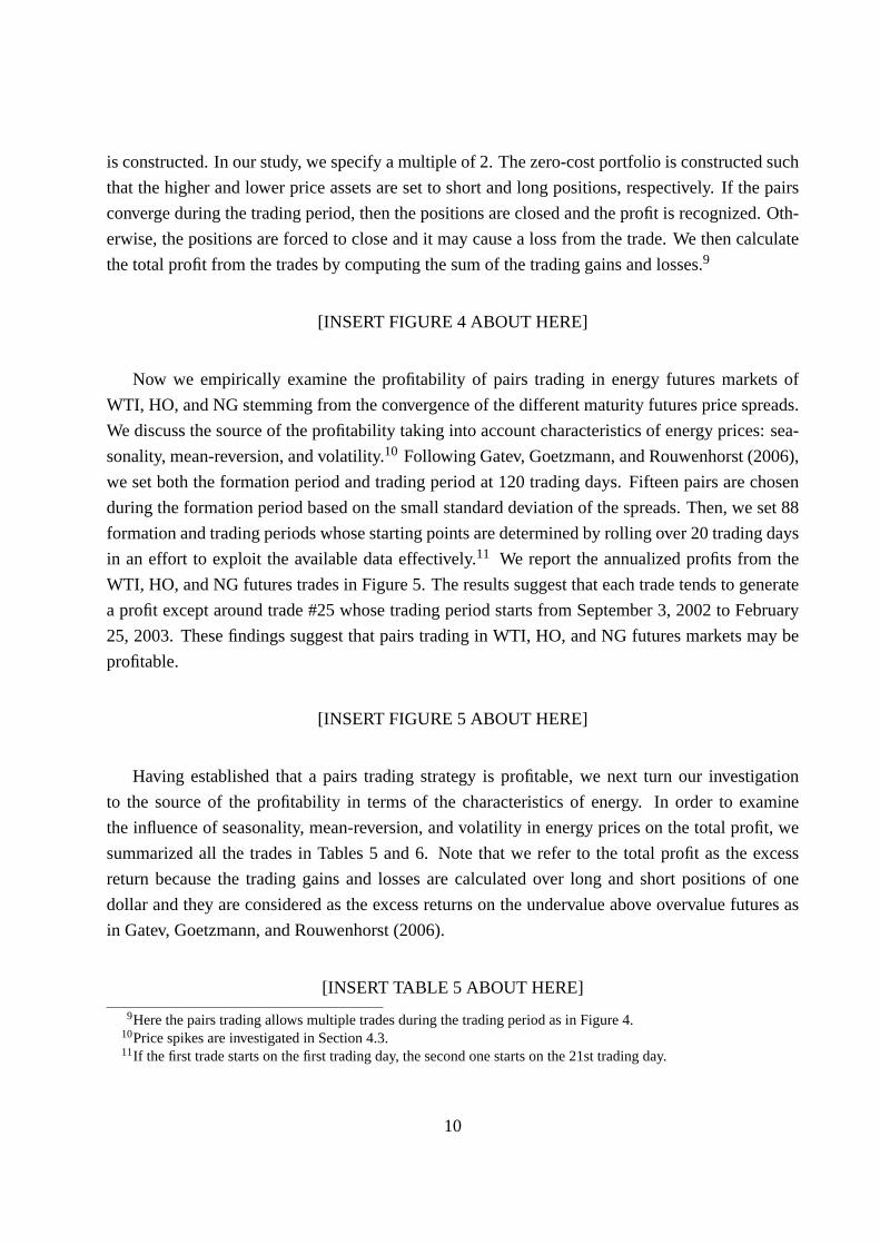
is constructed. In our study, we specify a multiple of 2. The zero-cost portfolio is constructed such
that the higher and lower price assets are set to short and long positions, respectively. If the pairs
converge during the trading period, then the positions are closed and the profit is recognized. Oth-
erwise, the positions are forced to close and it may cause a loss from the trade. We then calculate
the total profit from the trades by computing the sum of the trading gains and losses.9
[INSERT FIGURE 4 ABOUT HERE]
Now we empirically examine the profitability of pairs trading in energy futures markets of
WTI, HO, and NG stemming from the convergence of the different maturity futures price spreads.
We discuss the source of the profitability taking into account characteristics of energy prices: sea-
sonality, mean-reversion, and volatility.10 Following Gatev, Goetzmann, and Rouwenhorst (2006),
we set both the formation period and trading period at 120 trading days. Fifteen pairs are chosen
during the formation period based on the small standard deviation of the spreads. Then, we set 88
formation and trading periods whose starting points are determined by rolling over 20 trading days
in an effort to exploit the available data effectively.11 We report the annualized profits from the
WTI, HO, and NG futures trades in Figure 5. The results suggest that each trade tends to generate
a profit except around trade#25 whose trading period starts from September 3, 2002 to February
25, 2003. These findings suggest that pairs trading in WTI, HO, and NG futures markets may be
profitable.
[INSERT FIGURE 5 ABOUT HERE]
Having established that a pairs trading strategy is profitable, we next turn our investigation
to the source of the profitability in terms of the characteristics of energy. In order to examine
the influence of seasonality, mean-reversion, and volatility in energy prices on the total profit, we
summarized all the trades in Tables 5 and 6. Note that we refer to the total profit as the excess
return because the trading gains and losses are calculated over long and short positions of one
dollar and they are considered as the excess returns on the undervalue above overvalue futures as
in Gatev, Goetzmann, and Rouwenhorst (2006).
[INSERT TABLE 5 ABOUT HERE]
9Here the pairs trading allows multiple trades during the trading period as in Figure 4.10Price spikes are investigated in Section 4.3.11If the first trade starts on the first trading day, the second one starts on the 21st trading day.
10

[INSERT TABLE 6 ABOUT HERE]
First, we address the influence of seasonality of energy futures prices on the profit generated
from pairs trading by focusing on winter. To do this using a simple examination, we define “winter
trade” presented in Tables 5 and 6 by the trade including the days from December to February. In
Tables 5 and 6, the winter trades comprise eight periods: the trades from#1 to #4, from #12 to
#16, from #25to #29, from #37to #41, #50to #54, #62to #66, #75to #79, and#87to #88.
Table 5 shows that all winter trades of WTI, HO, and NG from#1 to #4 produce profits. From
#12 to #16, the trades of HO and NG produce profits, while the trades of WTI have annualized
losses of -0.36 and -0.09 for#12 and#13, respectively. The winter trades of WTI, HO, and NG
from #26 to #29produce profits.12 Accordingly, these findings for the winter trades suggest that
while the WTI trades produce both gains and losses in the winter, the HO and NG trades always
make profits in the winter. In addition, the trades of HO and NG in the summer from#5 to #8 and
from #17to #19produce low profits or losses while the WTI trades generate profits to some extent.
The same characteristics explained above are observed in the other winter trades in Tables 5 and
6. While the profits from the WTI trades are not relevant to the season, seasonality in profitability
from HO and NG trades exists in the sense that the trades of HO and NG in the winter tend to
cause high profits while those in the summer show low profits or losses. The results correspond
to the existence of seasonality explained in Pilipovic (1998) such that HO and NG futures prices
exhibit seasonality contrary to WTI futures prices.
Since we are interested in the influence of seasonality on the total profit from energy futures
pairs trading, we compared the annualized average profits between WTI, HO, and NG. According
to the results reported in Table 6, the profits from six WTI, HO, and NG futures trades are 0.61,
0.74, and 3.15, respectively. We found that the NG trading generates the largest total profits (i.e.,
the highest excess return) of the three contracts investigated during the trading periods as in Table
6, while the HO and the WTI showed the second and the third highest excess return, respectively.
Since the profits from the WTI trades without seasonality are less than those from the HO and NG
trades with seasonality, this factor may determine the total profit.
Second, we can shed light on the mean-reversion and volatility of the spread as the source of
the total profits from pairs trading. For all combinations of the spreads for each energy futures, we
estimate the parameters of AR(1) coefficientρ and standard deviationσ, which represent mean-
reversion strength and volatility, respectively, using equation (11). Then, we take the averageρandσ of the estimatedρ’s andσ’s, respectively, in order to capture the average trend of the mean-
reversion and volatility of each energy futures market. The results are shown in Table 7. As can
12Later in this paper we discuss trade#25as a special case.
11

be seen, the price spread of NG futures has the strongest mean-reversion and the highest volatility
of the three, because the AR(1) coefficient is the smallest (0.981) and the standard deviation is
the largest (0.257) of the three. Considering that the NG trades generate the highest average return
(3.15) of the three, the highest total profit of pairs trading applied to NG futures may come from the
strongest mean reversion and highest volatility of the spread. The comparative statics in Section
3.2 suggested that the strong mean-reversion and high volatility of price spreads may produce high
profit from pairs trading. Thus, the results obtained in this section may also be supported by the
results from the comparative statics.
[INSERT TABLE 7 ABOUT HERE]
As is discussed, the results from the empirical analyses document that strong mean-reversion
and high volatility of price spreads, as well as seasonality, may influence the total profit from pairs
trading of energy futures.
4.3. Pairs Trading and Event Risk
When we studied the influence of seasonality on the profit from pairs trading in the previous sec-
tion, trade#25 was not relevant to the seasonality-based profit in the sense that the HO and NG
trades exhibited huge losses in spite of winter trades. In this section, we attempt to explain the
reason for the exception by exploring the influence of event risk as measured by price spikes on
the profit from pairs trading.
We begin by examining the relationship between the risk and return for the trading strategy,
since price spikes may affect the relationship. We illustrate the return distributions of pairs trading
for three energy futures in Figure 6. The WTI trading achieves sustainable profits with small losses
as shown in the top part of Figure 6, because the distribution almost lies in the positive region and
the width of the distribution is the smallest of the three futures. It corresponds to the positive mean
(0.61) and the smallest variance (1.03) in Table 6. In contrast, the NG futures trading produces not
only large profits but also a large loss (-4.35) as shown in the bottom part of Figure 6, leading to
the largest variance (8.52) in Table 6. HO trading is in the middle in terms of the risk and return
relationship as shown in the middle part of Figure 6.
[INSERT FIGURE 6 ABOUT HERE]
In addition, we examined fat-tailed and skewed distributions for the returns by estimating the
well-known α-stable distribution parameters ofα, β, µ, andσ. The parameterα describes the
12

kurtosis of the distribution with0< α≤ 2. The smaller theα, the heavier the tail of the distribution.
The parameterβ describes the skewness of the distribution,−1≤ β≤ 1. If β is positive (negative),
then the distribution is skewed to the right (left).µ and σ are the shift and scale parameters,
respectively. Ifα andβ equal 2 and 0, respectively, then theα-stable distribution reduces to the
normal one. The estimation results are reported in Table 8. Sinceαs for WTI and NG are 2, both
return distributions do not have fat tails. On the other hand, sinceα for HO is 1.464, the return
distribution has a fat tail. Then, sinceβs for WTI, HO, and NG are 1, the distributions are all
skewed to the right. Thus, the returns to pairs trades in energy futures markets may more or less be
influenced by infrequent extreme loss, resulting in what economists refer to as the “peso problem,”
observed by Milton Friedman about the Mexican peso market of the early 1970s.
[INSERT TABLE 8 ABOUT HERE]
We next investigate the source of this huge loss by analyzing the price behavior of the pairs
in detail. The huge loss in NG futures trading occurs in trade#25 in Table 5, while the loss is
included in winter trades that are expected to produce profits due to seasonality. We illustrate the
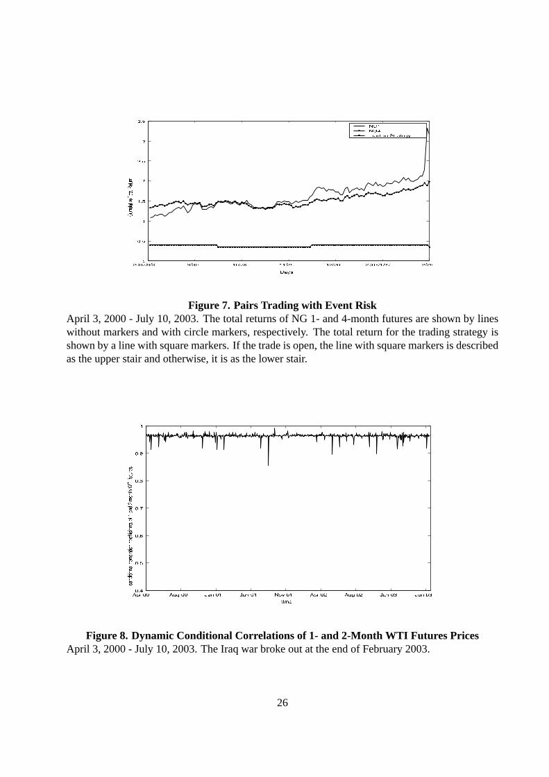
price movement of a typical pair for NG#25 trading in Figure 7 which shows the total returns of
NG 1- and 4-month futures by lines without markers and with circle markers, respectively. The
total return for the trading strategy is shown by a line with square markers. If the trade is open, the
line with square markers is described as the upper stair and otherwise, it is described as the lower
stair. According to Figure 7, after the position opens on December 11, 2002 due to the expansion
of price spread by more than two standard deviation in the formation period, the spread expands
dramatically just before the breakout of the Iraq war around the end of February 2003. The trading
position is forced to close without convergence at the end of the trading period. It gives rise to the
large loss from pairs trading. Therefore, the event risk expressed as price spikes may dramatically
adversely impact the relatively stable profit from NG futures pairs trading.
[INSERT FIGURE 7 ABOUT HERE]
13

In order to support the above observation of the impact of event risk, we will capture the
correlation structure of energy futures prices by using the dynamic conditional correlation (DCC)
model for pricespt (see Engle (2002)):13
pt = φ0 +φ1pt−1 + εt , (12)
εt = Dtηt , (13)
Dt = diag[h121t h
122t ], (14)
wherept = [p1,t p2,t ]′, φ0 = [φ1,0 φ2,0]′, andφ1 = [φ1,1 φ2,1]′.14 For i = 1, 2, we have
hit = ωi +αiε2i,t−1 +βihi,t−1, (15)
E[εtε′t | Ft−1] = DtRtDt , (16)
Rt = Q∗−1t QtQ
∗−1t , (17)
Qt = (1−θ1−θ2)Q+θ1ηt−1η′t−1 +θ2Qt−1, (18)
whereQ∗t is the diagonal component of the square root of the diagonal elements ofQt .15 Here,hit s
(i = 1,2) represent the GARCH(1,1) model for pair prices, respectively. The covariance matrixQt
is represented by the past noiseηt−1 and the past covariance matrixQt−1. If either of the estimates
of θ1 or θ2 in equation (18) is statistically significant, the correlationRt of the pairs becomes
time-varying.
We estimated the parameters of the DCC model and then calculated the conditional corre-
lations, employing 1- and 2-month maturity futures prices of the WTI, HO, and NG using the
sample data from April 3, 2000 to July 10, 2003 which covers trade#25.16 After the estimation
of the AR(1) model, we estimated the DCC model. The estimates of the parameters of the AR(1)
model for WTI, HO, and NG futures prices are reported in Table 9. Since all AR(1) parameters
in the table are statistically significant, there exist AR(1) effects both in the prices of 1- and 2-
month maturity futures prices for the three futures contracts. Next, we estimated the parameters of
13For pairs trading, since the correlations between price levels generate the profit, we examine the correlationsbetween prices assuming that the prices are mean reverting. However, the appendix to this paper also examines thecorrelations by using price returns and shows that the same results as reported in this section are obtained from theprice returns.
14It may be possible that the sample distribution of the innovationsηt is not normally distributed; however forsimplicity we assume that it is normally distributed and independent.
15DefineQt ≡(
q11 q12
q21 q22
). Then,Q∗
t =( √
q11 00
√q22
).
16We select 1- and 2-month maturity pairs in the sense that the spread may explicitly reflect the impact of eventrisk since the pairs may strongly move together due to the Samuelson effect such that the standard deviation of futuresprice returns decreases as the maturity increases (see Samuelson (1965)). The effect is especially pronounced in energymarkets.
14

the DCC model. The parameter estimation results and the conditional correlations for WTI, HO,
and NG are given in Table 10 and Figure 8, Table 11 and Figure 9, and Table 12 and Figure 10,
respectively.
[INSERT TABLE 9 ABOUT HERE]
[INSERT TABLE 10 ABOUT HERE]
[INSERT FIGURE 8 ABOUT HERE]
[INSERT TABLE 11 ABOUT HERE]
[INSERT FIGURE 9 ABOUT HERE]
[INSERT TABLE 12 ABOUT HERE]
[INSERT FIGURE 10 ABOUT HERE]
According to the standard errors ofθ1s andθ2s for WTI, HO, and NG as in Tables 10, 11, and
12, respectively, the conditional correlations of HO and NG are time-varying because theθ1, θ2, or
both are statistically significant. Judging from Figures 8, 9, and 10, the correlation of WTI futures
is high and stable, that of HO futures is volatile, and that of NG futures is high and stable except for
the first quarter 2003. By using these results, we discuss the relationship between the correlations
and event risk, where the Iraq war breaks out around the first three months of 2003. Figure 8
for WTI suggests that event risk does not seem to influence the correlations of the WTI futures
prices. Figure 9 for HO shows that event risk may more or less influence the correlations, while
we cannot distinguish the influence of event risk from the volatile correlations observed during
the entire trading period. However, Figure 10 for NG suggests that event risk strongly affects the
correlations, resulting in a small correlation (0.45) in February 2003. Judging from the analyses
using the DCC model, the trades of NG futures are the most vulnerable to event risk as measured
by price spikes, corresponding to the results in Table 6.17
Event risk captured as price spikes as in Figures 7 and 10 have a strong impact on the profit
from NG pairs trading. Thus the price spikes, one of the most well-known characteristics of energy
17We also estimated the DCC model for the three energy markets and obtained the conditional correlation using notthe price model in equation (12) but log price return model in equation (A1) of the appendix to this paper. The resultsare almost identical as the characteristics of the correlations obtained in this section.
15

prices, may also lead to the strong deterioration of the total profit from pairs trading which is
highlighted in the natural gas futures trades, depending on the magnitude and frequency of the
spikes.
4.4. Cross Commodities Pairs Trading
Finally, we investigate the profitability of cross commodities pairs trading that can also make use
of different commodity pairs such as 1-month NG and 6-month WTI futures in comparison to
the pairs trading of single commodity futures examined in Section 4.2. Here, we refer to the
improvement of profitability by cross commodities as the “portfolio effect,” while we refer to the
advantage in the profitability by single commodity as the “term structure convergence effect.” If
the total profit from cross commodities trading exceeds that from the sum of the three commodity
pairs trading in Table 6, the portfolio effect can improve the profits in pairs trading more than
the term structure convergence effect. We employ all combinations of WTI, HO, and NG futures
prices in Section 4.2 and choose the highly correlated 45 pairs in order to attain equal footing of
the profits from all the commodity trades in Section 4.2.18
The plots in Figure 11 show that cross commodity trading generated losses in the consecutive
periods from trades#22to #29and from trades#54to #61, while it almost produces profits from
trades#1 to #88except for several trades that are almost equal zero such as trade#2. This is dif-
ferent from single commodity pairs trading of NG in Figure 5 because the NG trades also generate
profits from the trades from#22to #29and from#54to #61.
[INSERT FIGURE 11 ABOUT HERE]
We then computed the total average profit of cross commodity pairs trading to be 3.04, while
the sum of single commodity trading profit from WTI, HO, and NG to be 4.50 as in Table 6. Our
findings suggest that the portfolio effect due to the cross commodity using three energy futures may
not improve the total profit of the pairs trading strategy, but the term structure convergence effect of
single commodity pairs trading can produce the profit from pairs trading in energy markets. This
result supports that the source of profits from energy futures pairs trading lies in the term structure
convergence of a single commodity.
In order to obtain a deeper understanding of the yield curve play, we examined the volatility
of three energy futures price returns illustrated in Figure 12. The figure shows that volatility
18Each commodity pairs trading introduces the selection of 15 pairs. Since cross commodity trading uses all threeenergy futures, it selects 45 pairs (three times as many as the selection for single commodity trades).
16
decreases in the maturity month, resulting in the Samuelson effect. According to Hong (2000), his
model predicts that the Samuelson effect holds in markets where information asymmetry among
investors is small. Thus, there may exist small information asymmetry among investors in the
three energy futures markets. In the presence of small information asymmetry, investors recognize
that the temporal supply shock observed in short maturity futures is just transient and dies out
quickly. Thus, long maturity futures are not affected by this temporal shock, meaning that the
price spread is only determined by the short-term futures price because the long-term futures price
almost remains constant. When the shock settles, the price spread may converge. This result also
supports our finding that the source of profits from energy futures pairs trading lies in the term
structure convergence of the energy futures market we study.
[INSERT FIGURE 12 ABOUT HERE]
In addition, Litzenberger and Rabinowitz (1995) showed that strong backwardation is posi-
tively correlated with the riskiness of futures prices. If this riskiness is captured by volatility,
backwardation may also be considered a source of profits from pairs trading in energy futures
markets.
5. Conclusions
In this paper we examine the usefulness of a hedge fund trading strategy known as “pairs trading”
as applied to energy futures markets, focusing on the characteristics of energy futures. The profit
of a simplified pairs trading strategy was modeled by using a mean-reverting process of energy
futures price spreads. The comparative statics of the expected return using the model indicated
that both strong mean reversion and high volatility of price spreads give rise to high expected
returns from pairs trading. Our empirical analyses using WTI crude oil, heating oil, and natural
gas futures traded on the NYMEX show that pairs trading in energy futures markets can produce a
relatively stable profit.
The sources of the total profit were investigated from the characteristics of energy futures
prices: strong seasonality, strong mean reversion, high volatility, and large price spikes. The total
profits from heating oil and natural gas trading were found to be positively affected by seasonality,
contrary to the WTI crude oil, resulting in the greater total profits of heating oil and natural gas
with seasonality than that of WTI crude oil without seasonality. Seasonality may seem to charac-
terize the total profit. Then, we examined the influence of mean reversion and volatility of price
spreads on the total profit. The results suggest that the strong mean reversion and high volatility
17
may cause high total profits from pairs trading, especially in natural gas trades. Moreover, event
risk, as measured by price spikes for pairs trading, were examined using Engle’s dynamic condi-
tional correlation model. The low correlations of natural gas futures prices with different maturities
were prominently observed during the first quarter of 2003 when the Iraq war broke out, contrary
to the other two energy futures. The results suggest that natural gas futures trades are the most
vulnerable of the three energy futures to event risk as measured by price spikes. Thus, price spikes
may also lead to the strong deterioration of the total profit from pairs trading.
Finally, we investigated the profitability of cross commodities pairs trading. We found that the
portfolio effect using cross commodities may not improve the profitability of pairs trading but the
term structure convergence effect of single commodity pairs trading produces the total profit from
pairs trading in energy markets.
18

Appendix. DCC Model for Price Returns
We model the log return of the pricesyt by using Engle’s dynamic conditional correlation (DCC) model as
follows:19
yt = εt , (A1)
εt = Dtηt , (A2)
Dt = diag[h121,th
122,t ], (A3)
whereyt = (y1,t ,y2,t)′, εt = (ε1,t ,ε2,t)′, andηt = (η1,t ,η2,t)′.
For i = 1, 2, we have
hi,t = ωi +αiε2i,t−1 +βihi,t−1, (A4)
E[εtε′t | Ft−1] = DtRtDt , (A5)
Rt = Q∗−1t QtQ
∗−1t , (A6)
Qt = (1−θ1−θ2)Q+θ1ηt−1η′t−1 +θ2Qt−1, (A7)
whereQ∗t is the diagonal component of the square root of the diagonal elements ofQt . Equation (A4)
represents a GARCH(1,1) effect for each price return. The conditional correlation is calculated as equation
(A6) where equation (A7) represents the time-varying conditional covariance. If either of the estimates of
θ1 or θ2 as in equation (A7) is statistically significant, the correlation structure of the pairs becomes time
varying.
We estimated the parameters of the DCC model for the price returns and then calculated the conditional
correlation by employing 1- and 2-month maturity futures prices of WTI, HO, and NG, respectively. The
estimates of the parameters and the conditional correlation for WTI, HO, and NG are given in Table 13 and
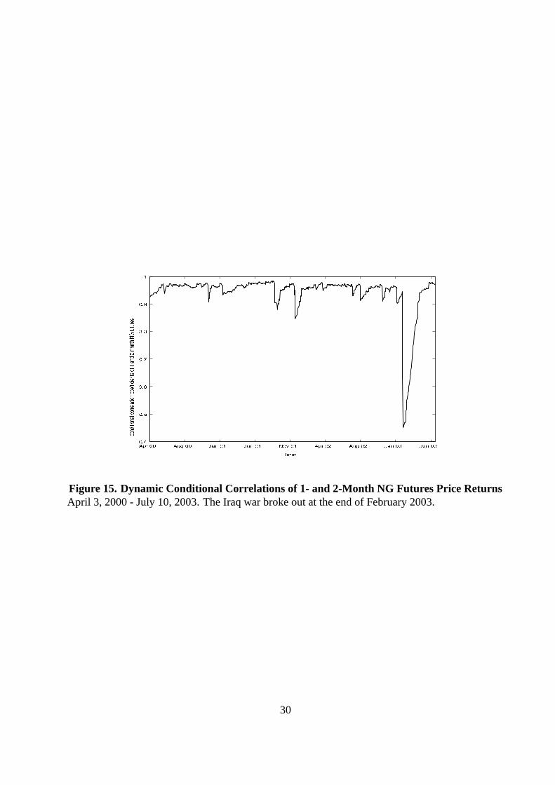
Figure 13, Table 14 and Figure 14, and Table 15 and Figure 15, respectively. Judging from Figures 13, 14,
and 15, the correlation of WTI futures is high and stable, that of HO futures is volatile, and that of NG
futures is high and stable except for the first quarter of 2003.
[INSERT TABLE 13 ABOUT HERE]
[INSERT FIGURE 13 ABOUT HERE]
[INSERT TABLE 14 ABOUT HERE]
19We estimated the AR(1) model foryt , but both the AR(1) coefficient and the constant terms were not statisticallysignificant. Thus, we model returns by equation (A1).
19
[INSERT FIGURE 14 ABOUT HERE]
[INSERT TABLE 15 ABOUT HERE]
[INSERT FIGURE 15 ABOUT HERE]
We next shed light on event risk where the Iraq war broke out during the first three months of 2003.
Figure 13 for WTI suggests that event risk does not seem to influence the correlation of WTI futures prices.
Although Figure 14 for HO suggests that event risk may more or less influence the correlation, we cannot
distinguish this influence from the volatile correlation during the entire observation period. However, Figure
15 for NG suggests that event risk strongly affects that of the NG trades. Thus, the analyses employing the
DCC model suggest that NG futures trades are the most vulnerable of the three energy futures to event risk,
agreeing with the results reported in Section 4.3.
20

References
Alexander, C., 1999, Correlation and cointegration in energy markets, in Vincent Kaminski, eds.:Managing
Energy Price Risk(Risk Publications, London ).
Dempster, M., E. Medova, and K. Tang, 2008, Long term spread option valuation and hedging, Working
paper, forthcoming inJournal of Money, Credit and Banking.
Engle, R.F., 2002, Dynamic conditional correlation: a new simple class of multivariate GARCH models,
Journal of Business and Economic Statistics20, 339–350.
Eydeland, A., and K. Wolyniec, 2003,Energy and Power Risk Management: New Developments in Model-
ing, Pricing, and Hedging (John Wiley & Sons, Inc. Hoboken).
Gatev, E.G., W. N. Goetzmann, and K. G. Rouwenhorst, 2006, Pairs Trading: Performance of a Relative-
Value Arbitrage Rule,Review of Financial Studies19, 797–827.
Hong, H., 2000, A model of returns and trading in futures markets,Journal of Finance55, 959–988.
Jurek, J., and H. Yang, 2007, Dynamic portfolio selection in arbitrage, Working paper, Harvard University.
Linetsky, V., 2004, Computing hitting time densities for CIR and OU diffusions: Applications to mean-
reverting models,Journal of Computational Finance7, 1–22.
Litzenberger, R. H., and N. Rabinowitz, 1995, Backwardation in oil futures markets: Theory and empirical
evidents,Journal of Finance50, 1517–1545.
Pilipovic, D., 1998,Energy Risk: Valuing and Managing Energy Derivatives (McGraw-Hill New York).
Samuelson, P.A., 1965, Proof that properly anticipated prices fluctuate randomly,Industrial Management
Review6, 41–49.
21

Figures& Tables
������������������
�����������������
��������
��
��
�
�
�
� �
� �
� �
�
��� ���������� � � �����������������
�� !"#$%&&' ()*
Figure 1. NYMEX Natural Gas Futures Curves
April 3, 2000 - March 31, 2008. NG futures product includes six delivery months – from one tosix months.
22

��� ����� ��� ������� ��� ����� ��� ������� ��� ����� ��� ������� ��� ������� �����
��� ����
��� ������
��� ����
��� ������
��� ����
��� ������
κ
����� ��� �� ���
Figure 2. Comparative Statics ofκ
By increasing the mean-reversionκ from 0.024 to 0.027 holding volatility constant at 0.0130, wecalculated the corresponding expected returns for the simple profit model.
��� ������� ��� ������� ��� ������� ��� ������ ��� ����� ��� ������ ��� ������� ��� ������� ��� ������ ��� �������� �����
��� �������
��� �����
��� �������
��� �����
��� �������
��� �����
σ
����� ��� �� ���
Figure 3. Comparative Statics ofσ
By increasing the volatilityσ from 0.0112 to 0.0130 holding mean-reversion constant at 0.027,the corresponding expected returns for the simple profit model are shown.
23
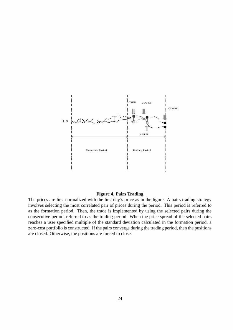
Figure 4. Pairs TradingThe prices are first normalized with the first day’s price as in the figure. A pairs trading strategyinvolves selecting the most correlated pair of prices during the period. This period is referred toas the formation period. Then, the trade is implemented by using the selected pairs during theconsecutive period, referred to as the trading period. When the price spread of the selected pairsreaches a user specified multiple of the standard deviation calculated in the formation period, azero-cost portfolio is constructed. If the pairs converge during the trading period, then the positionsare closed. Otherwise, the positions are forced to close.
24

� ��� ��� ��� ��� ��� ��� �� �� ���� �
� �
� �
�
�
�
�
���
���
���
����������������
� ������ �� !"#$"" %&' (�)*
+ �-,��/.�0/.������1 ����0/2 3�4���2 56�/.�0/.������7 ��0/.�����564����8�/.�0/.������
Figure 5. Pairs Trading of WTI Crude Oil, Heating Oil, and Natural Gas FuturesWe set 88 formation and trading periods whose starting points are determined by rolling over 20trading days. The first starting point is September 25, 2000 and the last (88th) point is September14, 2007.
� � ��� ��� � � � � � � � � ��
� �
���
� ��� �������������
� � ��� ��� � � � � � � � � ��
�
� �
������ �
������� ������� �������������
� � ��� ��� � � � � � � � � ��
�
� �
������
"!$# ���$�&%'����������(�)*��������� � +$��,�-
. �����������$�����������������
Figure 6. Returns Distributions of Pairs Trading for Three Energy Futures(1) For returns distributions from WTI futures trades, the mean is 0.61, the maximum is 3.47, theminimum is -1.09, the standard deviation is 1.01, the skewness is 0.63, and the kurtosis is 2.68.(2) For returns distributions from HO futures trades, the mean is 0.74, the maximum is 3.98, theminimum is -3.24, the standard deviation is 1.24, the skewness is 0.52, and the kurtosis is 3.94.(3) For returns distributions from NG futures trades, the mean is 3.15, the maximum is 10.61, theminimum is -4.35, the standard deviation is 2.92, the skewness is 0.36, and the kurtosis is 2.90.
25
��������������� ������� �������� �������� ��������� ��������������� ��������
��� �
�
��� �
�
��� �
�
��� �
�������
� ���� ��� ��� � ��! �� �"#
$&% �$&%(')+*,��-�. /�021435*,��356�0��
Figure 7. Pairs Trading with Event RiskApril 3, 2000 - July 10, 2003. The total returns of NG 1- and 4-month futures are shown by lineswithout markers and with circle markers, respectively. The total return for the trading strategy isshown by a line with square markers. If the trade is open, the line with square markers is describedas the upper stair and otherwise, it is as the lower stair.
��������� �������� ��� ��� ��� ��� ��������� ��������� �������� ��� ��� ��� ������ �
��� �
��� �
��� �
��� �
��� �
�
� � !"
#$%&' (' $%)*#$++,* )(' $%#$,--'#' ,%(.$-/)%&01$%(2345- 6( 6+,.
Figure 8. Dynamic Conditional Correlations of 1- and 2-Month WTI Futures PricesApril 3, 2000 - July 10, 2003. The Iraq war broke out at the end of February 2003.
26

��������� �������� ��� ��� ��� ��� ��������� ��������� �������� ��� ��� ��� ������ �
��� �
��� �
��� �
��� �
��� �
�
� � !"
#$%&' (' $%)*#$++,* )('$%#$,--'#' ,%( .$-/)%&01$%(234- 5( 5+,.
Figure 9. Dynamic Conditional Correlations of 1- and 2-Month HO Futures PricesApril 3, 2000 - July 10, 2003. The Iraq war broke out at the end of February 2003.
��������� �������� ��� ��� ��� ��� ��������� ��������� �������� ��� ��� ��� ������� �
��� �
��� �
��� �
��� �
��� �
�
� � !"
#$%&' (' $%)*#$++,* )('$%#$,--'#' ,%( .$-/)%&01$%(234- 5( 5+,.
Figure 10. Dynamic Conditional Correlations of 1- and 2-Month NG Futures PricesApril 3, 2000 - July 10, 2003. The Iraq war broke out at the end of February 2003.
27

� ��� ��� ��� ��� ��� ��� �� �� ���� ���
� ���
� ���
�
���
���
���
������������������ ����������� ��
! "# $%& '(')*'
Figure 11. Returns of Pairs Trading for Cross CommoditiesThere are 88 formation and trading periods whose starting points are determined by rolling over20 trading days. The first starting point is September 25, 2000 and the last (88th) is September 14,2007.
� � � � � ���� ����
��� ��
��� ���
��� ��
��� ���
��� ��
� ������� ����� �����
� �� ����� � �� !"� "#$%& #� '$( $� "#)
*,+.-/10243
Figure 12. Samuelson Effect in Energy Futures MarketsApril 3, 2000 - March 31, 2008. The volatility of price returns for WTI, HO, and NG futures –from one to six months, respectively, are shown.
28

��������� �������� ��� ��� ��� ��� ��������� ��������� �������� ��� ��� ��� ������ �
��� �
��� �
��� �
��� �
��� �
�
� � !"
#$%&' (' $%)*#$++,* )(' $%#$,--'#' ,%(.$-/)%&01$%(2345- 6( 6+,.
Figure 13. Dynamic Conditional Correlations of 1- and 2-Month WTI Futures Price ReturnsApril 3, 2000 - July 10, 2003. The Iraq war broke out at the end of February 2003.
��������� �������� ��� ��� ��� ��� ��������� ��������� �������� ��� ��� ��� ������� �
��� �
��� �
��� �
��� �
��� �
�
�! "#
$%&'( )( %&*+$%,,-+ *)(%&$%-..($( -&) /%.0*&'12%&)345. 6) 6,-/
Figure 14. Dynamic Conditional Correlations of 1- and 2-Month HO Futures Price ReturnsApril 3, 2000 - July 10, 2003. The Iraq war broke out at the end of February 2003.
29
��������� �������� ��� ��� ��� ��� ��������� ��������� �������� ��� ��� ��� ������ �
��� �
��� �
��� �
��� �
��� �
�
� � !"
#$%&' (' $%)*#$++,* )('$%#$,--'#' ,%( .$-/)%&01$%(234- 5( 5+,.
Figure 15. Dynamic Conditional Correlations of 1- and 2-Month NG Futures Price ReturnsApril 3, 2000 - July 10, 2003. The Iraq war broke out at the end of February 2003.
30

Variable C12 ρ12 C13 ρ13 C14 ρ14 C15 ρ15 C16 ρ16
Coefficient -0.152 0.957 -0.259 0.977 -0.303 0.985 -0.344 0.987 -0.363 0.989Std. Error 0.047 0.015 0.132 0.011 0.259 0.008 0.320 0.007 0.385 0.006Variable C23 ρ23 C24 ρ24 C25 ρ25 C26 ρ26 C34 ρ34
Coefficient -0.107 0.976 -0.151 0.985 -0.190 0.987 -0.210 0.989 -0.043 0.980Std. Error 0.077 0.012 0.213 0.009 0.278 0.007 0.362 0.006 0.126 0.018Variable C35 ρ35 C36 ρ36 C45 ρ45 C46 ρ46 C56 ρ56
Coefficient -0.082 0.984 -0.101 0.987 -0.039 0.976 -0.057 0.986 -0.017 0.973Std. Error 0.197 0.011 0.296 0.007 0.077 0.012 0.195 0.007 0.089 0.018
Table 1. AR(1) Models for Natural Gas Futures Price SpreadCi j andρi j denote the constant term and the first lag coefficient of AR(1) model for price spreads (Pi −P j )for i and j month natural gas futures (i 6= j).
WTI1 WTI2 WTI3 WTI4 WTI5 WTI6
Mean 45.96 46.03 45.99 45.87 45.71 45.55Median 37.21 36.47 35.91 35.44 34.99 34.53Maximum 110.33 109.17 107.94 106.90 106.06 105.44Minimum 17.45 17.84 18.06 18.27 18.44 18.60Std. Dev. 20.66 20.92 21.14 21.32 21.49 21.65Skewness 0.81 0.76 0.72 0.69 0.67 0.66Kurtosis 2.79 2.59 2.44 2.33 2.24 2.17
Table 2. Basic Statistics of WTI Crude Oil Futures PricesApril 3, 2000 - March 31, 2008. The maturity month is denoted by a subindex from one to sixmonths.
31

HO1 HO2 HO3 HO4 HO5 HO6
Mean 127.86 128.27 128.35 128.15 127.82 127.44Median 101.90 99.83 98.53 96.25 94.02 91.97Maximum 314.83 306.45 301.55 301.05 301.10 301.50Minimum 49.99 51.31 51.71 51.96 51.52 50.87Std. Dev. 59.54 60.28 60.98 61.52 61.93 62.30Skewness 0.73 0.68 0.65 0.64 0.63 0.62Kurtosis 2.58 2.37 2.21 2.11 2.04 2.00
Table 3. Basic Statistics of Heating Oil Futures PricesApril 3, 2000 - March 31, 2008. The maturity month is denoted by a subindex from one to sixmonths.
NG1 NG2 NG3 NG4 NG5 NG6
Mean 6.01 6.16 6.27 6.31 6.35 6.36Median 5.94 6.11 6.19 6.09 6.11 6.18Maximum 15.38 15.43 15.29 14.91 14.67 14.22Minimum 1.83 1.98 2.08 2.18 2.26 2.33Std. Dev. 2.27 2.32 2.36 2.34 2.33 2.30Skewness 0.90 0.90 0.90 0.73 0.60 0.39Kurtosis 4.75 4.72 4.57 3.83 3.28 2.43
Table 4. Basic Statistics of Natural Gas Futures PricesApril 3, 2000 - March 31, 2008. The maturity month is denoted by a subindex from one to sixmonths.
32

# Beginning End WTI HO NG Winter Trade1 09/25/00 03/19/01 1.98 1.64 2.61 Yes2 10/23/00 04/17/01 2.19 2.70 3.07 Yes3 11/20/00 05/15/01 2.88 3.67 5.58 Yes4 12/20/00 06/13/01 1.45 3.98 8.06 Yes5 01/22/01 07/12/01 1.85 0.49 0.34 No6 02/20/01 08/09/01 0.53 0.19 0.18 No7 03/20/01 09/07/01 0.55 0.19 0.16 No8 04/18/01 10/11/01 0.54 0.14 0.08 No9 05/16/01 11/08/01 0.15 0.29 0.11 No
10 06/14/01 12/10/01 0.08 0.24 0.49 No11 07/13/01 01/10/02 0.16 0.82 2.64 No12 08/10/01 02/08/02 -0.36 1.03 3.32 Yes13 09/10/01 03/11/02 -0.09 1.26 4.23 Yes14 10/12/01 04/09/02 1.00 1.01 1.10 Yes15 11/09/01 05/07/02 1.39 0.41 1.16 Yes16 12/11/01 06/05/02 3.47 0.03 0.06 Yes17 01/11/02 07/03/02 2.90 0.03 -0.25 No18 02/11/02 08/02/02 2.30 -0.12 -0.17 No19 03/12/02 08/30/02 2.61 -0.19 1.02 No20 04/10/02 09/30/02 1.96 0.25 2.67 No21 05/08/02 10/28/02 1.73 0.56 3.14 No22 06/06/02 11/25/02 1.79 0.54 4.30 No23 07/08/02 12/26/02 -0.01 -1.56 6.15 No24 08/05/02 01/27/03 0.62 -1.02 6.35 No25 09/03/02 02/25/03 -0.59 -3.24 -4.35 Yes26 10/01/02 03/25/03 1.10 1.74 3.14 Yes27 10/29/02 04/23/03 1.44 3.00 3.51 Yes28 11/26/02 05/21/03 1.47 3.04 3.34 Yes29 12/27/02 06/19/03 2.27 3.71 3.07 Yes30 01/28/03 07/18/03 1.67 2.83 4.03 No31 02/26/03 08/15/03 2.00 3.45 5.88 No32 03/26/03 09/15/03 0.25 0.01 0.67 No33 04/24/03 10/13/03 0.00 -0.11 -0.22 No34 05/22/03 11/10/03 0.00 -0.06 0.50 No35 06/20/03 12/10/03 0.00 -0.08 -1.78 No36 07/21/03 01/13/04 0.00 -0.14 2.16 No37 08/18/03 02/11/04 0.00 0.71 3.67 Yes38 09/16/03 03/11/04 0.04 2.08 4.52 Yes39 10/14/03 04/08/04 0.70 2.16 4.62 Yes40 11/11/03 05/07/04 0.70 2.37 3.33 Yes41 12/11/03 06/07/04 1.04 2.57 5.40 Yes42 01/14/04 07/07/04 1.01 2.69 0.41 No43 02/13/04 08/04/04 1.32 0.02 0.02 No44 03/12/04 09/01/04 1.10 -0.10 0.26 No45 04/12/04 09/30/04 1.04 0.06 3.26 No
Table 5. Excess Returns from Pairs Trading and Seasonality“Winter trade” is defined to be trades including the days from December to February. The winter trades inthis table comprise four periods: the trades from#1 to #4, from #12to #16, from #25to #29, and from#37to #41.
33

# Beginning End WTI HO NG Winter Trade46 05/10/04 10/28/04 1.06 -0.04 4.54 No47 06/08/04 11/29/04 0.90 -0.53 7.72 No48 07/08/04 12/28/04 -0.07 -0.21 6.24 No49 08/05/04 01/27/05 -0.09 0.24 7.73 No50 09/02/04 02/25/05 -0.27 1.16 10.26 Yes51 10/01/04 03/28/05 -0.87 2.51 5.39 Yes52 10/29/04 04/25/05 -1.09 2.36 3.48 Yes53 11/30/04 05/23/05 -1.08 2.75 0.19 Yes54 12/29/04 06/21/05 -0.74 0.34 0.00 Yes55 01/28/05 07/20/05 -1.02 -0.36 0.00 No56 02/28/05 08/17/05 -0.65 -0.39 0.13 No57 03/29/05 09/15/05 -0.33 -0.28 2.68 No58 04/26/05 10/13/05 0.45 0.08 5.65 No59 05/24/05 11/10/05 0.14 0.02 5.96 No60 06/22/05 12/12/05 -0.23 0.24 2.57 No61 07/21/05 01/11/06 0.08 1.08 10.41 No62 08/18/05 02/09/06 -0.26 0.70 6.33 Yes63 09/16/05 03/10/06 -0.49 0.92 5.44 Yes64 10/14/05 04/07/06 -0.58 0.73 5.34 Yes65 11/11/05 05/08/06 -0.39 0.33 4.38 Yes66 12/13/05 06/06/06 -0.05 -0.15 4.80 Yes67 01/12/06 07/05/06 -0.06 -0.53 -0.26 No68 02/10/06 08/02/06 0.31 -0.26 2.86 No69 03/13/06 08/30/06 0.22 -0.59 2.99 No70 04/10/06 09/28/06 -0.22 -0.60 5.34 No71 05/09/06 10/26/06 -0.26 -0.17 7.40 No72 06/07/06 11/24/06 -0.46 0.36 8.59 No73 07/06/06 12/22/06 -0.29 0.83 10.61 No74 08/03/06 01/25/07 -0.19 1.11 6.20 No75 08/31/06 02/23/07 -0.14 1.57 6.58 Yes76 09/29/06 03/23/07 0.09 1.58 1.75 Yes77 10/27/06 04/23/07 0.43 1.01 0.00 Yes78 11/27/06 05/21/07 0.30 0.47 0.00 Yes79 12/26/06 06/19/07 0.42 0.45 0.00 Yes80 01/26/07 07/18/07 1.33 0.00 0.05 No81 02/26/07 08/15/07 1.48 0.16 0.66 No82 03/26/07 09/13/07 2.11 0.55 0.72 No83 04/24/07 10/11/07 1.84 0.42 1.99 No84 05/22/07 11/09/07 2.10 0.51 3.36 No85 06/20/07 12/07/07 1.26 0.41 4.31 No86 07/19/07 01/09/07 0.41 0.72 5.56 No87 08/16/07 02/06/07 -0.05 1.05 4.29 Yes88 09/14/07 03/06/07 0.09 1.08 2.82 YesAverage Excess Return 0.61 0.74 3.15Variance of the Return 1.03 1.53 8.52
Table 6. Excess Returns from Pairs Trading and Seasonality (Cont’d)“Winter trade” is defined to be trades including the days from December to February. The winter trades inthis table comprise four periods: from#50to #54, from #62to #66, from #75to #79, and from#87to #88.
34
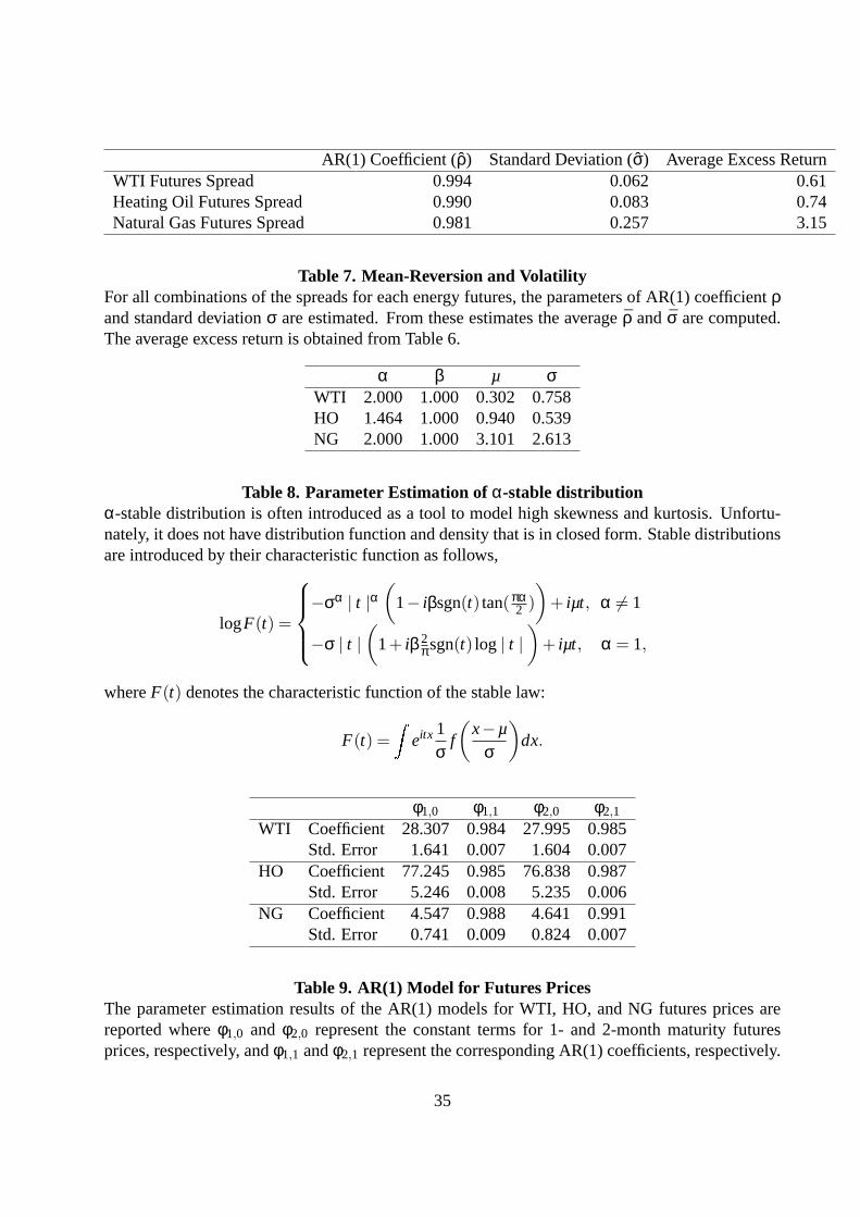
AR(1) Coefficient (ρ) Standard Deviation (σ) Average Excess ReturnWTI Futures Spread 0.994 0.062 0.61Heating Oil Futures Spread 0.990 0.083 0.74Natural Gas Futures Spread 0.981 0.257 3.15
Table 7. Mean-Reversion and VolatilityFor all combinations of the spreads for each energy futures, the parameters of AR(1) coefficientρand standard deviationσ are estimated. From these estimates the averageρ andσ are computed.The average excess return is obtained from Table 6.
α β µ σWTI 2.000 1.000 0.302 0.758HO 1.464 1.000 0.940 0.539NG 2.000 1.000 3.101 2.613
Table 8. Parameter Estimation ofα-stable distributionα-stable distribution is often introduced as a tool to model high skewness and kurtosis. Unfortu-nately, it does not have distribution function and density that is in closed form. Stable distributionsare introduced by their characteristic function as follows,
logF(t) =
−σα | t |α(
1− iβsgn(t) tan(πα2 )
)+ iµt, α 6= 1
−σ | t |(
1+ iβ 2πsgn(t) log | t |
)+ iµt, α = 1,
whereF(t) denotes the characteristic function of the stable law:
F(t) =Z
eitx 1σ
f
(x−µ
σ
)dx.
φ1,0 φ1,1 φ2,0 φ2,1
WTI Coefficient 28.307 0.984 27.995 0.985Std. Error 1.641 0.007 1.604 0.007
HO Coefficient 77.245 0.985 76.838 0.987Std. Error 5.246 0.008 5.235 0.006
NG Coefficient 4.547 0.988 4.641 0.991Std. Error 0.741 0.009 0.824 0.007
Table 9. AR(1) Model for Futures PricesThe parameter estimation results of the AR(1) models for WTI, HO, and NG futures prices arereported whereφ1,0 and φ2,0 represent the constant terms for 1- and 2-month maturity futuresprices, respectively, andφ1,1 andφ2,1 represent the corresponding AR(1) coefficients, respectively.
35
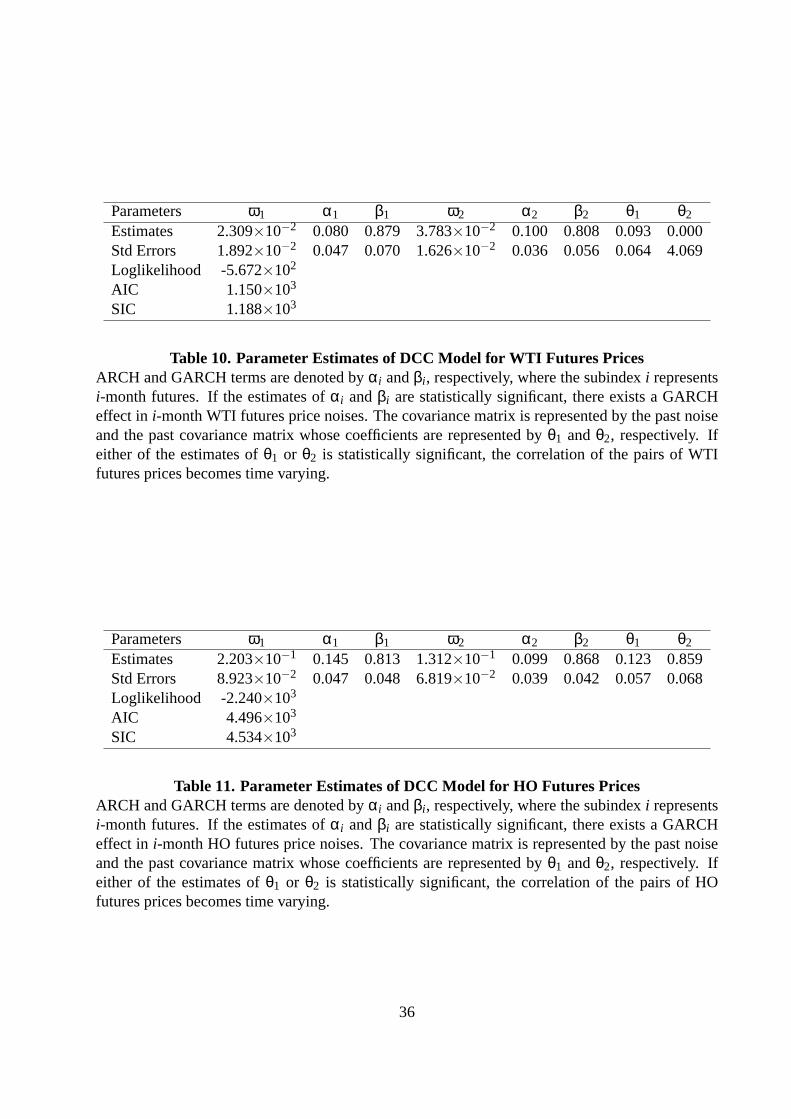
Parameters ω1 α1 β1 ω2 α2 β2 θ1 θ2
Estimates 2.309×10⁻² 0.080 0.879 3.783×10⁻² 0.100 0.808 0.093 0.000Std Errors 1.892×10⁻² 0.047 0.070 1.626×10⁻² 0.036 0.056 0.064 4.069Loglikelihood -5.672×10²
AIC 1.150×10³
SIC 1.188×10³
Table 10. Parameter Estimates of DCC Model for WTI Futures PricesARCH and GARCH terms are denoted byαi andβi , respectively, where the subindexi representsi-month futures. If the estimates ofαi andβi are statistically significant, there exists a GARCHeffect in i-month WTI futures price noises. The covariance matrix is represented by the past noiseand the past covariance matrix whose coefficients are represented byθ1 andθ2, respectively. Ifeither of the estimates ofθ1 or θ2 is statistically significant, the correlation of the pairs of WTIfutures prices becomes time varying.
Parameters ω1 α1 β1 ω2 α2 β2 θ1 θ2
Estimates 2.203×10⁻¹ 0.145 0.813 1.312×10⁻¹ 0.099 0.868 0.123 0.859Std Errors 8.923×10⁻² 0.047 0.048 6.819×10⁻² 0.039 0.042 0.057 0.068Loglikelihood -2.240×10³
AIC 4.496×10³
SIC 4.534×10³
Table 11. Parameter Estimates of DCC Model for HO Futures PricesARCH and GARCH terms are denoted byαi andβi , respectively, where the subindexi representsi-month futures. If the estimates ofαi andβi are statistically significant, there exists a GARCHeffect in i-month HO futures price noises. The covariance matrix is represented by the past noiseand the past covariance matrix whose coefficients are represented byθ1 andθ2, respectively. Ifeither of the estimates ofθ1 or θ2 is statistically significant, the correlation of the pairs of HOfutures prices becomes time varying.
36

Parameters ω1 α1 β1 ω2 α2 β2 θ1 θ2
Estimates 2.956×10⁻³ 0.365 0.635 1.231×10⁻³ 0.150 0.812 0.036 0.944Std Errors 1.400×10⁻³ 0.213 0.132 4.356×10⁻⁴ 0.036 0.035 0.070 0.016Loglikelihood 1.448×10³
AIC -2.881×10³
SIC -2.843×10³
Table 12. Parameter Estimates of DCC Model for NG Futures PricesARCH and GARCH terms are denoted byαi andβi , respectively, where the subindexi representsi-month futures. If the estimates ofαi andβi are statistically significant, there exists a GARCHeffect in i-month NG futures price noises. The covariance matrix is represented by the past noiseand the past covariance matrix whose coefficients are represented byθ1 andθ2, respectively. Ifeither of the estimates ofθ1 or θ2 is statistically significant, the correlation of the pairs of NGfutures prices becomes time varying.
Parameters ω1 α1 β1 ω2 α2 β2 θ1 θ2
Estimates 5.187×10⁻⁵ 0.087 0.841 0.000 0.104 0.807 0.011 0.974Std Errors 2.672×10⁻⁵ 0.042 0.060 0.000 0.040 0.054 0.064 0.205Loglikelihood 4.818×10³
AIC -9.621×10³
SIC -9.583×10³
Table 13. Parameter Estimates of DCC Model for WTI Futures Price ReturnsARCH and GARCH terms are denoted byαi andβi , respectively, where the subindexi representsi-month futures. If the estimates ofαi andβi are statistically significant, there exists a GARCHeffect ini-month WTI futures price return noises. The covariance matrix is represented by the pastnoise and the past covariance matrix whose coefficients are represented byθ1 andθ2, respectively.If either of the estimates ofθ1 or θ2 is statistically significant, the correlation of the pairs of WTIfutures price returns becomes time varying.
37
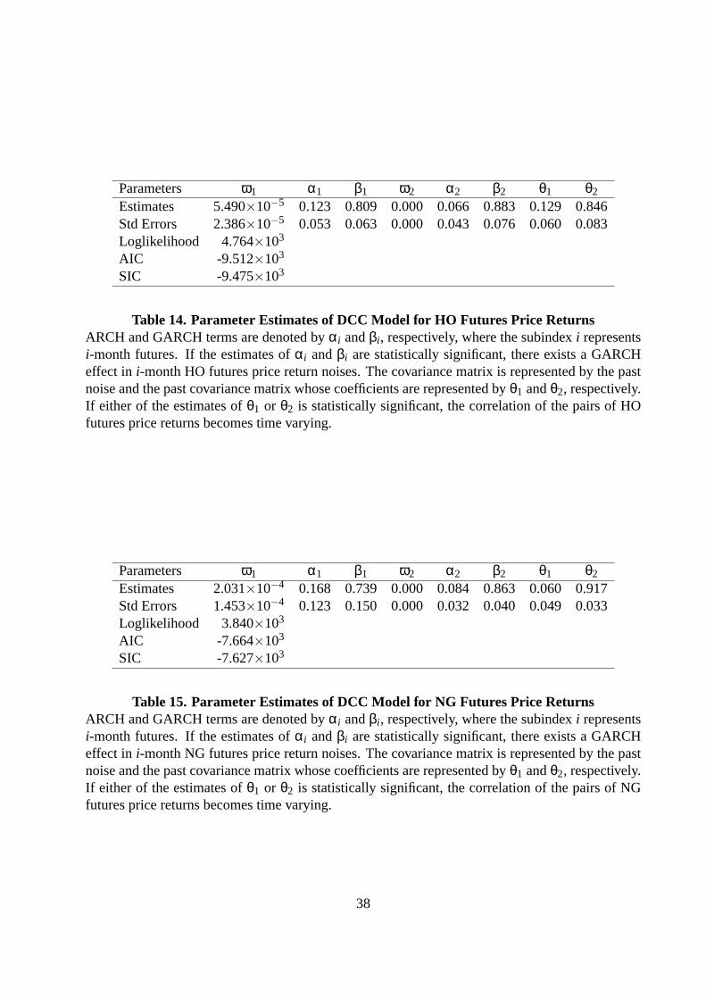
Parameters ω1 α1 β1 ω2 α2 β2 θ1 θ2
Estimates 5.490×10⁻⁵ 0.123 0.809 0.000 0.066 0.883 0.129 0.846Std Errors 2.386×10⁻⁵ 0.053 0.063 0.000 0.043 0.076 0.060 0.083Loglikelihood 4.764×10³
AIC -9.512×10³
SIC -9.475×10³
Table 14. Parameter Estimates of DCC Model for HO Futures Price ReturnsARCH and GARCH terms are denoted byαi andβi , respectively, where the subindexi representsi-month futures. If the estimates ofαi andβi are statistically significant, there exists a GARCHeffect in i-month HO futures price return noises. The covariance matrix is represented by the pastnoise and the past covariance matrix whose coefficients are represented byθ1 andθ2, respectively.If either of the estimates ofθ1 or θ2 is statistically significant, the correlation of the pairs of HOfutures price returns becomes time varying.
Parameters ω1 α1 β1 ω2 α2 β2 θ1 θ2
Estimates 2.031×10⁻⁴ 0.168 0.739 0.000 0.084 0.863 0.060 0.917Std Errors 1.453×10⁻⁴ 0.123 0.150 0.000 0.032 0.040 0.049 0.033Loglikelihood 3.840×10³
AIC -7.664×10³
SIC -7.627×10³
Table 15. Parameter Estimates of DCC Model for NG Futures Price ReturnsARCH and GARCH terms are denoted byαi andβi , respectively, where the subindexi representsi-month futures. If the estimates ofαi andβi are statistically significant, there exists a GARCHeffect in i-month NG futures price return noises. The covariance matrix is represented by the pastnoise and the past covariance matrix whose coefficients are represented byθ1 andθ2, respectively.If either of the estimates ofθ1 or θ2 is statistically significant, the correlation of the pairs of NGfutures price returns becomes time varying.
38