Pairs Trading Profits

in Commodity Futures Markets

Robert J. Bianchi a∗, Michael E. Drew b and Roger Zhu a

a. School of Economics and Finance

Queensland University of Technology GPO Box 2434

Brisbane, Queensland, 4001 Australia

b. Department of Accounting, Finance and Economics Griffith Business School

Griffith University Nathan, Queensland, 4111

Australia

January 2009

Abstract This study employs a pairs trading investment strategy on daily commodity futures returns. The study reveals that pairs trading in similarly related commodity futures earns statistically significant excess returns with commensurate volatility. The excess returns from pairs trading in commodity futures are unrelated to conventional market risk factors and they are not associated with classic contrarian investing. The evidence of pairs trading profits in commodity futures supports the view that these profits reflect compensation to arbitrageurs for enforcing the law of one price in similarly related markets to ensure market efficiency.

∗ Corresponding author: Email: r.bianchi@qut.edu.au; Tel: +61‐7‐3138 2951; Fax: +61‐7‐3138‐1500. We thank Adam Clements and Stan Hurn for helpful discussions and comments. Any remaining errors are our own.

Introduction

Pairs trading (and sometimes known as ‘statistical arbitrage’ or ‘stat arb’) has been a recognised investment strategy for many years within the professional investment community, however, it has received little research attention. The concept of pairs trading is the simultaneous buying and selling of two closely related markets to form a zero‐cost portfolio when these two markets are temporarily mispriced. Profits are realised when the prices of the two markets converge. The study by Gatev, Goetzmann and Rouwenhorst (2006) represents the pre‐eminent contribution in the academic literature which demonstrates empirical evidence of excess returns from pairs trading when applied to US stocks. Gatev et al (2006) find that excess returns from pairs trading are unrelated to market risk factors nor can they be explained by return‐reversal (see Lehmann (1990) and Jegadeesh (1990)) or contrarian investment strategies. (see DeBondt and Thaler (1985)).

Gatev et al (2006) argue that the important economic principle of the Law of One Price explains these arbitrage profits. The Law of One Price (LOP) states that close economic substitutes (such as two banking stocks) will exhibit similar payoffs, therefore, securities or markets which are similar will exhibit similar pricing. Gatev et al (2006) argue that the excess returns from pairs trading reflects profits earned by arbitrageurs in enforcing the LOP whilst ensuring that market efficiency. If arbitrage profits can be captured through pairs trading in stocks, then, the economic principle of LOP may be observed in other actively traded markets where close economic substitutes are also transacted?

A fertile empirical setting to test the presence of arbitrage profits from LOP is commodity futures markets. There are two motivations to empirically test pairs trading in global commodity futures. The work of von Hagen (1989) shows that unrelated commodities over eight decades tend to exhibit statistically significant cointegration which is a hypothesis test for joint stationarity.1 Gatev et al (2006) suggest that cointegrated markets are an important feature to ensure convergence between prices which are necessary to earn pairs trading profits. To support this strand of literature, Pindyck and Rotemberg (1990) have shown that seemingly unrelated monthly commodity prices in wheat, cotton, copper, gold, crude, lumber and cocoa tend to exhibit co‐movement. These empirical studies in commodities suggest that perfect economic substitutes (eg. London versus New York gold) are not necessary for co‐movement and cointegration to occur. These studies suggest that cointegration and co‐movement is present across the broad range of markets, regardless of observing perfect or imperfect economic substitutes in commodity markets which is consistent with the finding from Gatev et al (2006). This finding provides a conducive setting to empirically test whether excess returns are earned by arbitrageurs by enforcing the LOP through pairs trading in commodity futures markets.

1 Other works by Karbuz and Jumah (2006) report cointegration between cocoa and coffee while Booth and Ciner (2001) report similar evidence of cointegration in corn and soybeans.

This study makes three contributions to pairs trading research. First, we empirically test the LOP in commodity futures returns. If arbitrageurs enforce the LOP in stocks with pairs trading, then the same economic principle should be observed in other markets of where markets trade perfect and imperfect economic substitutes. To support the notion that pairs trading reflects excess returns garnered by arbitrageurs in enforcing the LOP, we examine this naïve investment strategy in a commodity futures market setting.

Second, we examine the source of excess returns from pairs trading in commodity futures. We investigate whether the source of pairs trading returns is attributable to conventional commodity market risk factors. This analysis allows us to consider whether the excess returns from pairs trading is truly an excess return earned by arbitrage profits for enforcing the LOP or perhaps it reflects a profit that is earned by being exposed to an observable commodity market risk factor.

Third, we examine whether excess returns from pairs trading is simply compensation for a conventional contrarian investment strategy. Studies by DeBondt and Thaler (1985), Lehmann (1990) and Jegadeesh (1990) argue that overreaction and return‐reversal effects are observed in stock returns. Whilst no such theoretical framework exists for return‐reversal or overreaction effects in commodities, this study empirically tests whether a dependence exists between the excess returns from pairs trading and a conventional contrarian investment strategy in commodity futures. This empirical examination allows us to determine whether the excess returns from pairs trading reflects the compensation to arbitrageurs for enforcing the LOP or whether pairs trading profits simply captures a contrarian investment strategy in commodity futures markets.

Over a sample period from 1990‐2007 on daily commodity futures returns, this study finds the evidence of statistically significant excess returns in pairs trading. The findings from this study reveal that these excess returns earned by arbitrageurs are subject to commensurate levels of volatility, therefore, these profits are not risk‐free due to the Shleifer and Vishny (1997) limits of arbitrage. Overall, this study supports the view that excess returns from pairs trading exist in both stocks and commodity futures markets which reflects the compensation of arbitrageurs for enforcing the LOP. An examination of the source of these excess returns reveals that these profits are not dependent upon conventional commodity market risk factors. Furthermore, the excess returns from pairs trading in commodity futures are found to be unrelated to conventional contrarian investment strategies. Overall, this study demonstrates that the rent earned by arbitrageurs in enforcing the LOP is not only observable in stock returns, it can also be captured in commodity futures returns also.

In the following section of the paper, we describe the data employed in the study, followed by the presentation of methodology and results. The final section of the paper provides a summary and our conclusions.

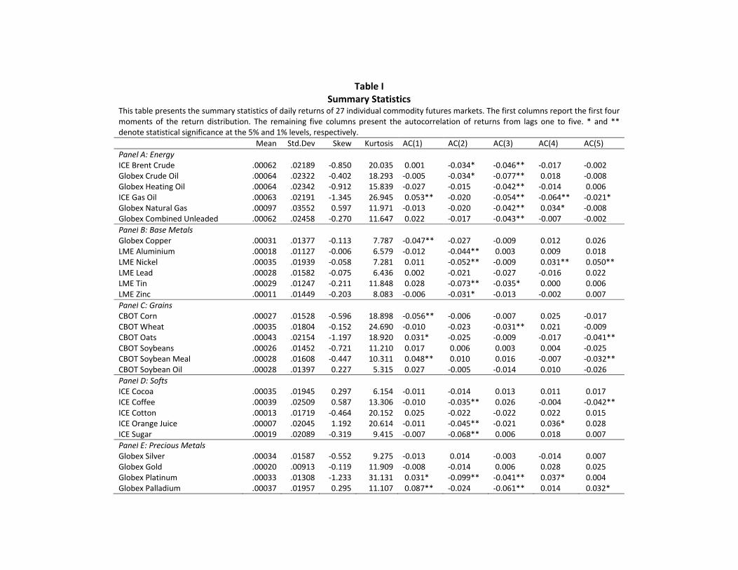
Table I Summary Statistics

This table presents the summary statistics of daily returns of 27 individual commodity futures markets. The first columns report the first four moments of the return distribution. The remaining five columns present the autocorrelation of returns from lags one to five. * and ** denote statistical significance at the 5% and 1% levels, respectively. Mean Std.Dev Skew Kurtosis AC(1) AC(2) AC(3) AC(4) AC(5)Panel A: Energy ICE Brent Crude .00062 .02189 ‐0.850 20.035 0.001 ‐0.034* ‐0.046** ‐0.017 ‐0.002Globex Crude Oil .00064 .02322 ‐0.402 18.293 ‐0.005 ‐0.034* ‐0.077** 0.018 ‐0.008Globex Heating Oil .00064 .02342 ‐0.912 15.839 ‐0.027 ‐0.015 ‐0.042** ‐0.014 0.006ICE Gas Oil .00063 .02191 ‐1.345 26.945 0.053** ‐0.020 ‐0.054** ‐0.064** ‐0.021*Globex Natural Gas .00097 .03552 0.597 11.971 ‐0.013 ‐0.020 ‐0.042** 0.034* ‐0.008Globex Combined Unleaded .00062 .02458 ‐0.270 11.647 0.022 ‐0.017 ‐0.043** ‐0.007 ‐0.002Panel B: Base Metals Globex Copper .00031 .01377 ‐0.113 7.787 ‐0.047** ‐0.027 ‐0.009 0.012 0.026LME Aluminium .00018 .01127 ‐0.006 6.579 ‐0.012 ‐0.044** 0.003 0.009 0.018LME Nickel .00035 .01939 ‐0.058 7.281 0.011 ‐0.052** ‐0.009 0.031** 0.050**LME Lead .00028 .01582 ‐0.075 6.436 0.002 ‐0.021 ‐0.027 ‐0.016 0.022LME Tin .00029 .01247 ‐0.211 11.848 0.028 ‐0.073** ‐0.035* 0.000 0.006LME Zinc .00011 .01449 ‐0.203 8.083 ‐0.006 ‐0.031* ‐0.013 ‐0.002 0.007Panel C: Grains CBOT Corn .00027 .01528 ‐0.596 18.898 ‐0.056** ‐0.006 ‐0.007 0.025 ‐0.017CBOT Wheat .00035 .01804 ‐0.152 24.690 ‐0.010 ‐0.023 ‐0.031** 0.021 ‐0.009CBOT Oats .00043 .02154 ‐1.197 18.920 0.031* ‐0.025 ‐0.009 ‐0.017 ‐0.041**CBOT Soybeans .00026 .01452 ‐0.721 11.210 0.017 0.006 0.003 0.004 ‐0.025CBOT Soybean Meal .00028 .01608 ‐0.447 10.311 0.048** 0.010 0.016 ‐0.007 ‐0.032**CBOT Soybean Oil .00028 .01397 0.227 5.315 0.027 ‐0.005 ‐0.014 0.010 ‐0.026Panel D: Softs ICE Cocoa .00035 .01945 0.297 6.154 ‐0.011 ‐0.014 0.013 0.011 0.017ICE Coffee .00039 .02509 0.587 13.306 ‐0.010 ‐0.035** 0.026 ‐0.004 ‐0.042**ICE Cotton .00013 .01719 ‐0.464 20.152 0.025 ‐0.022 ‐0.022 0.022 0.015ICE Orange Juice .00007 .02045 1.192 20.614 ‐0.011 ‐0.045** ‐0.021 0.036* 0.028ICE Sugar .00019 .02089 ‐0.319 9.415 ‐0.007 ‐0.068** 0.006 0.018 0.007Panel E: Precious Metals Globex Silver .00034 .01587 ‐0.552 9.275 ‐0.013 0.014 ‐0.003 ‐0.014 0.007Globex Gold .00020 .00913 ‐0.119 11.909 ‐0.008 ‐0.014 0.006 0.028 0.025Globex Platinum .00033 .01308 ‐1.233 31.131 0.031* ‐0.099** ‐0.041** 0.037* 0.004Globex Palladium .00037 .01957 0.295 11.107 0.087** ‐0.024 ‐0.061** 0.014 0.032*

Data Description

The study employs daily returns that are estimated from closing prices from 27 commodity futures markets from January 1990 to August 2008. For each futures market, the nearby futures contract was employed and rollovers into the next contract occurred on the last day of the month before contract expiration. The daily return on rollover days were based on the same futures contract in order to avoid percentage return distortions when rolling between futures contracts. For the London Metals Exchange (LME), the daily rolling three month forward market prices were employed on zinc, tin, lead, nickel and aluminium as it provided the most accurate independent process to estimate a daily rate of return from these contracts. From these returns, a daily index was constructed for this study. Table I presents the summary statistics of daily returns of the futures markets employed in this study. The futures markets are presented and classified by their respective commodity sector classification. The first column of Table 1 reports the daily mean returns, and in all cases, the first moment of the distribution is positive with Natural Gas reporting the highest daily mean return of 0.00097% whilst Orange Juice exhibiting the lowest daily mean return of 0.00007%. Overall, energy based markets exhibit the highest average returns while softs based markets report the lowest mean returns. The second column of Table I reports the daily standard deviation of returns. Natural Gas reports the highest daily standard deviation of 3.552% while Gold exhibits the lowest daily standard deviation at 0.913%. An important feature is the differences in the daily standard deviations between the various markets. Whilst the energy markets report some of the highest standard deviation, there are few obvious patterns or linkages from observing the volatility of returns. The third column of Table I reports the skewness statistic which shows that 21 of the 27 futures markets report negative symmetry in the distribution of daily returns. An interesting feature is that three of the six markets with positive skewness are cocoa, coffee and orange juice which are commodities in the softs sector. Column 4 of Table I reports the kurtosis measure which suggests that daily returns are fatter than expected under the assumption of normality. Although not reported, the Jarque‐Bera tests reject the normality assumption at the 1% level for all markets. To investigate whether returns are independent and identically distributed (iid), Columns 5 to 9 in Table I report the autocorrelation coefficients with lags ranging from one to five periods. A distinct feature in Table I is the statistically significant negative autocorrelation in lags two and three in many markets. This type of autocorrelation structure is consistent with the convergence behaviour of arbitrageurs purchasing undervalued and selling overvalued commodities with the expectation of the two markets converging.

Methodology

The research methodology adopted in this study predominantly follows Gatev et al. (2006) although modifications are employed to address the unique aspects relating to commodity futures. Pairs trading strategies seek to transact a pair of commodities based on the long‐term relationship between two closely related markets. The pairs investment strategy will sell short the winning market which is considered to be temporarily overvalued and buy the losing market which is considered to be temporarily undervalued. The pairs are formed during the formation period and the commodities futures markets are traded over the trading period after the formation of pairs.

Formation Period: To classify commodity markets into their respective pairs, we depart from the Gatev et al (2006) selection criteria and we propose an alternative method for constructing pairs. To avoid the possibility of data snooping bias, we segregate the markets into five distinct sector groups which are classified as energy, base metals, agricultural, precious metals and softs commodity sectors. These categories are typical classifications that reflect the close intrinsic economic relationships of these similarly related markets. This simple classification criteria mitigates the possibility of data snooping when pairs are constructed from erroneous relationships that are due to chance alone. The classification of each commodity futures market into the sector groups results in six markets in the Energy sector which form 15 pairs; six markets in the Base Metals classification which form 15 pairs; six markets in the Agricultural group which form 15 pairs; four markets in the Precious Metals sector which form 6 pairs, and finally, five markets in the Softs grouping which form 10 pairs. The formation period is used to describe the historical relationship between the commodities and the statistics in this time period provide the entry and exit points for the commencement of the trading period. The formation period is set to twelve months as adopted in Gatev et al. (2006). The purpose of the formation period is to design and construct the closeness measure which is employed to facilitate the comparison between the short‐term deviation and the long‐term behaviour of each commodity pair. Prior to the calculation of the closeness measure, the continuously compounded commodity futures contract return is calculated and the cumulative total returns index for each commodity is constructed. The cumulative total returns index is also described as the normalised commodity price (NCP).2

2 Let’s assume that the normalised commodity price commences at 1. If the log return of the subsequent day is 0.1, then the normalised commodity price will be 1.10. If the log return of the subsequent day is ‐0.1 then the normalised commodity price will be 0.90.

Trading Period: After the twelve month formation period, the entry and exit signals of each pair are transacted in the trading period. The Gatev et al (2006) methodology specifies a limited length for the trading period in order to re‐calculate a formation period which selects a new universe of highly related pairs of stocks. In this study, the universe of pairs is established based on their pre‐determined classification within each commodity sector, therefore, there is no need to limit the trading period as in Gatev et al (2006). Contrary to Gatev et al (2006), this study does not limit the length of the trading period as there is no need to re‐calculate a new set of pairs. The entry and exit points for opening and closing a transaction in each pair is determined with the daily normalised price spread (NPS) over the initial twelve months formation period which is calculated as:3

BtNCPA

tNCPABtNPS −= (1)

The standard deviation of the daily NPS is then calculated over the formation period. As in Gatev et al (2006), the entry point of the pairs trade is set as two standard deviations of the NPS. If the absolute value of the NPS in the trading period is greater than the trigger point, then a pairs position will be opened. Based on the above rules, it is possible to have three scenarios when transacting two commodities named A and B. The three possible scenarios are (i) short commodity A and long commodity B if the NPS is greater than 2 standard deviations at the end of the formation period (ii) long commodity A and short commodity B if the NPS is less than ‐2 standard deviations of the NPS at the end of the formation period; and (iii) no position open if the NPS is estimated within the ‐2 to +2 standard deviation range. The exit point or the closure of the pairs trade is determined as the crossover of the NCPs between the two commodities in an open position. Hence, (i) if a position is short commodity A and long commodity B, it will be closed when the NPS is equal or less than zero. (ii) Conversely, if a position is long commodity A and short commodity B, it will be closed when the NPS is equal or greater than zero. Figure 1 in the Technical Appendix illustrates the normalised price movement of the Brent Crude and Gas Oil pair during the trading period from August 1990 to December 1990. [RB, fix the graph] The top two lines represent the normalised price paths for the two commodities and the bottom line represents the opening and closing of the strategy on a daily basis. The trigger point was reached when the NPS between the two commodities was greater than the 2 standard deviations of the historical NPS over the formation period. Therefore a position was opened at day 15. The position remained open and closed on day 32 as the normalised prices crossed over. The second open position was established on day 73. Since there is no crossover of the normalised prices during the period specified in this example, the position remained open during the remaining period.

3 If the NCP for commodity A is 1.2 and NCP for commodity B is 1.1, then the normalised price spread of commodity A and B is the difference between the two NCPs.

Excess Return Calculation: A pairs trading transaction simultaneously purchases a commodity futures contract and sells short the futures contract in the second market.4 A typical pairs trading strategy is considered as a self‐financing strategy therefore the returns from pairs trading are excess returns over and above the risk‐free rate of return. Pairs trades can open and close position multiple times during the trading period and each cash flow generated is reinvested into the next trade. Therefore, the excess return is calculated based on the reinvested payoffs of each trade. Gatev et al. (2006) suggest that this is a conservative approach to calculate pairs trading returns because it implicitly assumes that the cash flows generated by each trade do not accumulate time value or earn interest. As the strategy consists of a simultaneous long and short position, the return of a pairs trading position is calculated as the sum of the equally weighted returns of the two positions:

A1tNCPA

tNCPreturnpositionlongDaily −−= (2)

)B1tNCPB

t(NCPreturnpositionshortDaily −−−=

(3)

returnpositionshortreturnposition longreturn PairsDaily += (4) This study employs continuously compounded daily returns and the positions of each trade are effectively marked‐to‐market daily. The daily returns of all positions are then aggregated to compute monthly continuous returns for subsequent regressions that are explained later in this study. The monthly continuous returns are then converted to discrete returns as the return analysis for portfolios in this study are based on monthly discrete returns. Portfolio Returns: We follow Gatev et al (2006) by calculating the returns of each pair trade and then aggregating them into various portfolios, namely, All Pairs, Top 5, Top 15 and for each commodity sector. The construction and calculation of the portfolio returns in this study follows Gatev et al. (2006) and adopts the two methods of (i) the commited capital portfolio and (ii) the fully invested capital portfolio approaches. The committed capital portfolio method allocates capital according to the total number of pairs available for trading including both opened and unopened pairs. The fully invested capital portfolio method allocates capital only by the number of pairs

4 This assumes that the pairs trader/arbitrageur develops an equal notional position in both commodity futures markets.

that are open during the trading period. The fully invested capital portfolio method is considered to be more aggressive while the committed capital portfolio method is considered to be more conservative. The primary difference between the two portfolio allocations is that the committed capital portfolio method allocates funds to the pairs that may not necessarily exhibit open positions during the trading period, therefore, pairs positions that are open are allocated less capital than the fully invested capital method. Pairs Selection:

The Gatev et al (2006) methodology employs a ’closeness’ measure to evaluate a pair’s relatedness to each other. The closeness measure is the sum of squared deviations of the normalized commodity price (NCP) for the two commodities in the pair over the entire 12‐month formation period and is expressed as:

2)BtNCP

DaysTrading ofNumber the

1tAt(NCPABCloseness −∑

== (5)

Gatev et al (2006) conduct the study on hundreds of stocks and only the stocks which report the minimised value of sum of squared deviations between each other are employed to form pairs. In this commodity futures study, we avoid the potential of data snooping bias by forcing each commodity to be a pair with each market within its commodity sector group. In this study, we employ the closeness measure to determine the Top 5 and Top 15 pairs that are most closely related to each other over the sample period. Trading Costs and Bid/Ask Bounce: To examine the robustness of pairs trading profits, Gatev et al (2006) adopt a one day waiting rule to enter and exit the markets in order to account for trading costs and the bid/ask bounce. It is well recognised that futures transaction costs are lower and equity markets are subject to much larger short selling and commission costs than commodity markets. As mentioned in the literature review, short selling restrictions are not imposed in commodity futures markets and commission costs are minimal. This study considers transaction costs from an institution investor’s viewpoint which are likely to be very low. It is important to recognise that institutional investors require to post initial margins, the rolling of futures contracts before maturity and funding of margin calls. Furthermore, commodity futures contract prices are still subject to the bid/ask bounce problem due to the inability to buy at the bid price and sell at the ask price. Miffre and Rallis (2007) argue that the roll‐over of futures contracts and margin risks should not be overstated and should be partially offset by not including the cash returns earned from the notional value of the futures contracts. This study does not address the risks associated with roll‐over of contracts and margin risks. However, the bid/ask bounce problem is significant and this study accounts for the problem by employing the one day waiting rule.

The ‘one day waiting’ rule documented in Gatev et al. (2006) provides a conservative assessment of returns. The one day waiting rule assumes an extreme case where the prices of the winner at the first divergence are ask prices and the loser are bid prices. If the next day prices are equally likely to be at the bid or ask, then delaying trades by one day will reduce the excess returns on average by half the sum of the spreads of the winner and the loser. If at the second convergence of the pairs, the winner is trading at the bid‐price and the loser at the ask‐price, the one day waiting rule will reduce the excess returns on average again by one‐half of the sum of the bid‐ask spreads of both stocks. This study employs the one day waiting rule whereby the trade is executed on the next business day’s closing price for every entry and exit signal. If pairs trading strategies remain profitable under these conservative assumptions, then it can be inferred that pairs trading strategies in commodity futures should be profitable after transaction costs. The implementation of the one day waiting rule in this study serves a third purpose which relates to nonsynchronous effects in global futures markets. This study employs some markets that are traded in Europe whilst a majority of commodity futures are predominantly traded in the USA time zone. The reality of this time zone difference is that an entry or exit signal may not be transacted in the market until the close of the following day which represents the prices employed by the one day waiting rule. These delays in trading are captured by the one day waiting rule which allows the results from these tests to reflect realistic transactional effects. Identification of the Source of Pairs Trading Excess Returns: It is of interest to the literature to identify the source of the variation of returns if pairs trading profits are statistically significant. Gatev et al. (2006) suggest that pairs trading in stocks are market neutral strategies as they do not exhibit a dependence with stock related risk factors. In this study, it is important to examine whether excess returns from commodity pairs trading are subject to any commodity related market risk factors or whether a factor to explain these returns cannot be identified. In this study, we examine the source of commodity pairs trading profits by regressing the pairs trading returns against a variety of market related commodity returns. To identify the potential source of excess returns from pairs trading, we aggregate the daily return of all pairs within each commodity sector to compute a commodity sector portfolio return which represents the systematic return from that commodities group.

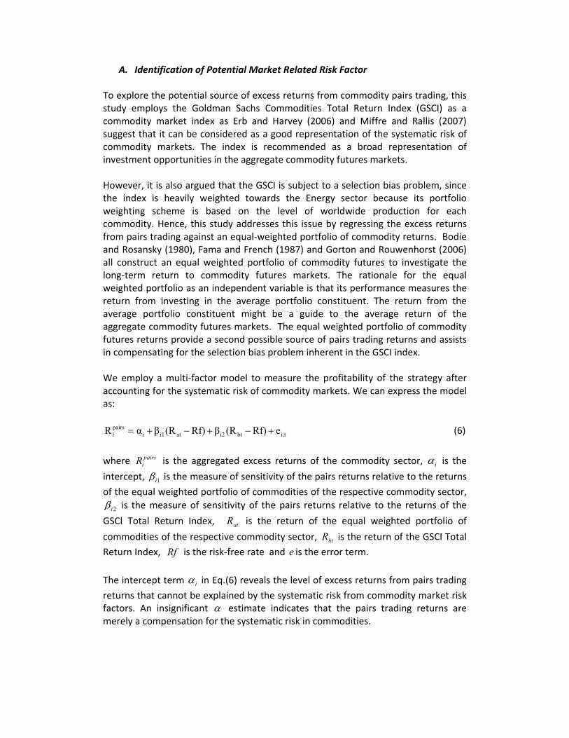
A. Identification of Potential Market Related Risk Factor To explore the potential source of excess returns from commodity pairs trading, this study employs the Goldman Sachs Commodities Total Return Index (GSCI) as a commodity market index as Erb and Harvey (2006) and Miffre and Rallis (2007) suggest that it can be considered as a good representation of the systematic risk of commodity markets. The index is recommended as a broad representation of investment opportunities in the aggregate commodity futures markets. However, it is also argued that the GSCI is subject to a selection bias problem, since the index is heavily weighted towards the Energy sector because its portfolio weighting scheme is based on the level of worldwide production for each commodity. Hence, this study addresses this issue by regressing the excess returns from pairs trading against an equal‐weighted portfolio of commodity returns. Bodie and Rosansky (1980), Fama and French (1987) and Gorton and Rouwenhorst (2006) all construct an equal weighted portfolio of commodity futures to investigate the long‐term return to commodity futures markets. The rationale for the equal weighted portfolio as an independent variable is that its performance measures the return from investing in the average portfolio constituent. The return from the average portfolio constituent might be a guide to the average return of the aggregate commodity futures markets. The equal weighted portfolio of commodity futures returns provide a second possible source of pairs trading returns and assists in compensating for the selection bias problem inherent in the GSCI index. We employ a multi‐factor model to measure the profitability of the strategy after accounting for the systematic risk of commodity markets. We can express the model as:

ti,bti2ati1ipairs eRf)(RβRf)(RβαR +−+−+=i (6)

where pairs

iR is the aggregated excess returns of the commodity sector, iα is the

intercept, 1iβ is the measure of sensitivity of the pairs returns relative to the returns

of the equal weighted portfolio of commodities of the respective commodity sector,

2iβ is the measure of sensitivity of the pairs returns relative to the returns of the

GSCI Total Return Index, atR is the return of the equal weighted portfolio of

commodities of the respective commodity sector, btR is the return of the GSCI Total

Return Index, Rf is the risk‐free rate and e is the error term. The intercept term iα in Eq.(6) reveals the level of excess returns from pairs trading

returns that cannot be explained by the systematic risk from commodity market risk factors. An insignificant α estimate indicates that the pairs trading returns are merely a compensation for the systematic risk in commodities.

B. Contrarian Returns as an Explanatory Variable of Excess Returns

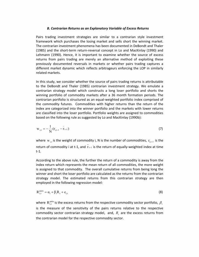
Pairs trading investment strategies are similar to a contrarian style investment framework which purchases the losing market and sells short the winning market. The contrarian investment phenomena has been documented in DeBondt and Thaler (1985) and the short‐term return‐reversal concept in Lo and MacKinlay (1990) and Lehmann (1990). Hence, it is important to examine whether the source of excess returns from pairs trading are merely an alternative method of exploiting these previously documented reversals in markets or whether pairs trading captures a different market dynamic which reflects arbitrageurs enforcing the LOP in similarly related markets. In this study, we consider whether the source of pairs trading returns is attributable to the DeBondt and Thaler (1985) contrarian investment strategy. We emulate a contrarian strategy model which constructs a long loser portfolio and shorts the winning portfolio of commodity markets after a 36 month formation periods. The contrarian portfolio is structured as an equal‐weighted portfolio index comprised of the commodity futures. Commodities with higher returns than the return of the index are categorized into the winner portfolio and the markets with lower returns are classified into the loser portfolio. Portfolio weights are assigned to commodities based on the following rule as suggested by Lo and MacKinlay (1990b):

)r(rN1w 1t1ti,ti, −− −−= (7)

where ti,w is the weight of commodity i, N is the number of commodities, 1ti,r − is the

return of commodity i at t‐1, and 1tr − is the return of equally‐weighted index at time t‐1. According to the above rule, the further the return of a commodity is away from the index return which represents the mean return of all commodities, the more weight is assigned to that commodity. The overall cumulative returns from being long the winner and short the loser portfolio are calculated as the returns from the contrarian strategy model. The estimated returns from this contrarian strategy are then employed in the following regression model:

ti,tiipairs

ti, eRβαR ++= (8)

where pairs

ti,R is the excess returns from the respective commodity sector portfolio, iβ is the measure of the sensitivity of the pairs returns relative to the respective commodity sector contrarian strategy model, and, tR are the excess returns from

the contrarian model for the respective commodity sector.

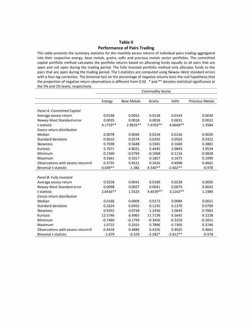
Table II Performance of Pairs Trading

This table presents the summary statistics for the monthly excess returns of individual pairs trading aggregated into their respective energy, base metals, grains, softs and precious metals sector portfolios. The committed capital portfolio method calculates the portfolio returns based on allocating funds equally to all pairs that are open and not open during the trading period. The fully invested portfolio method only allocates funds to the pairs that are open during the trading period. The t‐statistics are computed using Newey–West standard errors with a four‐lag correction. The binomial test on the percentage of negative returns tests the null hypothesis that the proportion of negative return observations is different from 0.50. * and ** denotes statistical significance at the 5% and 1% levels, respectively. Commodity Sector Energy Base Metals Grains Softs Precious Metals Panel A: Committed Capital Average excess return 0.0148 0.0052 0.0138 0.0143 0.0030Newey‐West Standard error 0.0035 0.0018 0.0018 0.0031 0.0022t‐statistic 4.1759** 2.9625** 7.6703** 4.6668** 1.3584Excess return distribution Median 0.0078 0.0044 0.0134 0.0126 0.0020Standard deviation 0.0610 0.0274 0.0392 0.0503 0.0322Skewness 0.7698 0.5648 0.5581 0.1669 0.3881Kurtosis 5.7071 4.8031 5.4445 2.9843 3.9534Minimum ‐0.1560 ‐0.0793 ‐0.1068 ‐0.1116 ‐0.0828Maximum 0.2661 0.1017 0.1857 0.1675 0.1099Observations with excess return<0 0.3735 0.4521 0.3426 0.4098 0.4661Binomial t‐statistic ‐3.649** ‐1.382 ‐4.540** ‐2.602** ‐0.978 Panel B: Fully Invested Average excess return 0.0258 0.0041 0.0189 0.0228 0.0050Newey‐West Standard error 0.0098 0.0027 0.0041 0.0073 0.0042t‐statistic 2.6416** 1.5525 4.6539** 3.1163** 1.1984Excess return distribution Median 0.0166 0.0009 0.0172 0.0084 0.0021Standard deviation 0.1624 0.0452 0.1142 0.1379 0.0709Skewness 0.9352 0.0728 1.2436 1.0645 0.7063Kurtosis 12.5746 6.4965 11.7139 6.5642 9.2228Minimum ‐0.7460 ‐0.1793 ‐0.3456 ‐0.3210 ‐0.2651Maximum 1.0722 0.2015 0.7896 0.7305 0.3746Observations with excess return<0 0.4418 0.4886 0.4105 0.4025 0.4661Binomial t‐statistic ‐1.679 ‐0.329 ‐2.582* ‐2.812** ‐0.978

Results

A. Excess Returns of Pairs Trading Strategies Table II presents the excess returns of the pairs trading strategies aggregated in their respective commodity sectors portfolios. The summary statistics in Table II report both committed capital and fully invested portfolio methods with the one day waiting rule which allows a comparison of the two types of capital allocations to be examined. This study proceeds with an emphasis on the results from the committed capital portfolio method as it is regarded as a more conservative approach to estimating the performance of pairs trading. The excess returns reported in Table II are statistically significant with the exception of the Precious Metals sector. The t‐statistics are sufficiently large even with the inclusion of Newey and West (1987) standard errors. The most profitable commodity group is the Energy sector which yields a statistically significant excess return of 1.48% per month. The least profitable commodity group is Precious Metals which exhibit 0.50% per month and is not statistically significant. Table II also presents the standard deviation of returns which tend to be very high in comparison to the mean excess returns. This is an important observation as it demonstrates that excess returns from pairs trading are not risk‐free and represent a premium to the arbitrageur for enforcing the LOP. Similar to the results of Gatev et al (2006), Table II reports positive skewness and relatively high kurtosis metrics across all commodity sector portfolio returns. Finally, the pairs trading profits in each sector exhibit daily losses which are less than 50%. The binomial test reports statistically significant t‐statistics for energy, grains and softs commodity sector portfolios which suggests that positive daily returns being observed in a majority of these commodity portfolios is not due to chance. Overall, the results in Table II demonstrate the presence of excess return in commodities pairs trading for nearly all commodity sectors. We now proceed to employ the ‘closeness measure’ to select the ‘Top 5’ and ‘Top 15’ portfolios of the best pairs and we also aggregate every pair into a fully diversified ‘All Pairs’ portfolio so that we can evaluate the performance and risk characteristics of these pair combinations.

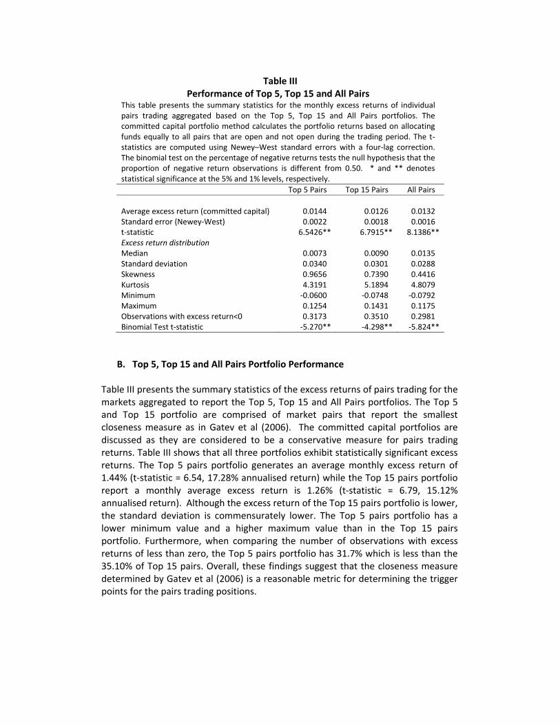
Table III

Performance of Top 5, Top 15 and All PairsThis table presents the summary statistics for the monthly excess returns of individual pairs trading aggregated based on the Top 5, Top 15 and All Pairs portfolios. The committed capital portfolio method calculates the portfolio returns based on allocating funds equally to all pairs that are open and not open during the trading period. The t‐statistics are computed using Newey–West standard errors with a four‐lag correction. The binomial test on the percentage of negative returns tests the null hypothesis that the proportion of negative return observations is different from 0.50. * and ** denotes statistical significance at the 5% and 1% levels, respectively. Top 5 Pairs Top 15 Pairs All Pairs Average excess return (committed capital) 0.0144 0.0126 0.0132 Standard error (Newey‐West) 0.0022 0.0018 0.0016 t‐statistic 6.5426** 6.7915** 8.1386** Excess return distribution Median 0.0073 0.0090 0.0135 Standard deviation 0.0340 0.0301 0.0288 Skewness 0.9656 0.7390 0.4416 Kurtosis 4.3191 5.1894 4.8079 Minimum ‐0.0600 ‐0.0748 ‐0.0792 Maximum 0.1254 0.1431 0.1175 Observations with excess return<0 0.3173 0.3510 0.2981 Binomial Test t‐statistic ‐5.270** ‐4.298** ‐5.824**

B. Top 5, Top 15 and All Pairs Portfolio Performance

Table III presents the summary statistics of the excess returns of pairs trading for the markets aggregated to report the Top 5, Top 15 and All Pairs portfolios. The Top 5 and Top 15 portfolio are comprised of market pairs that report the smallest closeness measure as in Gatev et al (2006). The committed capital portfolios are discussed as they are considered to be a conservative measure for pairs trading returns. Table III shows that all three portfolios exhibit statistically significant excess returns. The Top 5 pairs portfolio generates an average monthly excess return of 1.44% (t‐statistic = 6.54, 17.28% annualised return) while the Top 15 pairs portfolio report a monthly average excess return is 1.26% (t‐statistic = 6.79, 15.12% annualised return). Although the excess return of the Top 15 pairs portfolio is lower, the standard deviation is commensurately lower. The Top 5 pairs portfolio has a lower minimum value and a higher maximum value than in the Top 15 pairs portfolio. Furthermore, when comparing the number of observations with excess returns of less than zero, the Top 5 pairs portfolio has 31.7% which is less than the 35.10% of Top 15 pairs. Overall, these findings suggest that the closeness measure determined by Gatev et al (2006) is a reasonable metric for determining the trigger points for the pairs trading positions.

The characteristics of the return distributions of the Top 5, Top 15 and All Pairs portfolios are consistent with the aggregated excess returns reported earlier in the commodity sector portfolios. Table III shows that these portfolios exhibit positive skewness and high kurtosis relative to the normal distribution. During the full sample period, pairs trading strategies generate negative daily returns approximately one third of the time. When comparing the trading statistics of the Top 15 pairs portfolio against the All Pairs portfolio, it is interesting to note that the excess returns of the Top 15 pairs are very similar to the excess returns of the All Pairs portfolio, however the standard deviation of the All Pairs portfolio is much lower. It can be observed that the standard deviation falls as the number of pairs in a portfolio increases. This finding supports Gatev et al. (2006) who argue that there are diversification benefits from combining multiple pairs in a portfolio.

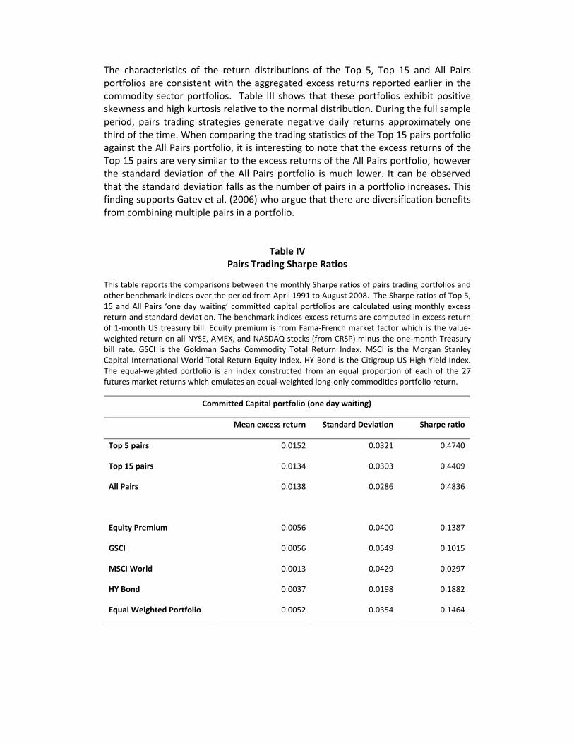
Table IV Pairs Trading Sharpe Ratios

This table reports the comparisons between the monthly Sharpe ratios of pairs trading portfolios and other benchmark indices over the period from April 1991 to August 2008. The Sharpe ratios of Top 5, 15 and All Pairs ‘one day waiting’ committed capital portfolios are calculated using monthly excess return and standard deviation. The benchmark indices excess returns are computed in excess return of 1‐month US treasury bill. Equity premium is from Fama‐French market factor which is the value‐weighted return on all NYSE, AMEX, and NASDAQ stocks (from CRSP) minus the one‐month Treasury bill rate. GSCI is the Goldman Sachs Commodity Total Return Index. MSCI is the Morgan Stanley Capital International World Total Return Equity Index. HY Bond is the Citigroup US High Yield Index. The equal‐weighted portfolio is an index constructed from an equal proportion of each of the 27 futures market returns which emulates an equal‐weighted long‐only commodities portfolio return.

Committed Capital portfolio (one day waiting)

Mean excess return Standard Deviation Sharpe ratio

Top 5 pairs 0.0152 0.0321 0.4740

Top 15 pairs 0.0134 0.0303 0.4409

All Pairs 0.0138 0.0286 0.4836

Equity Premium 0.0056 0.0400 0.1387

GSCI 0.0056 0.0549 0.1015

MSCI World 0.0013 0.0429 0.0297

HY Bond 0.0037 0.0198 0.1882

Equal Weighted Portfolio 0.0052 0.0354 0.1464

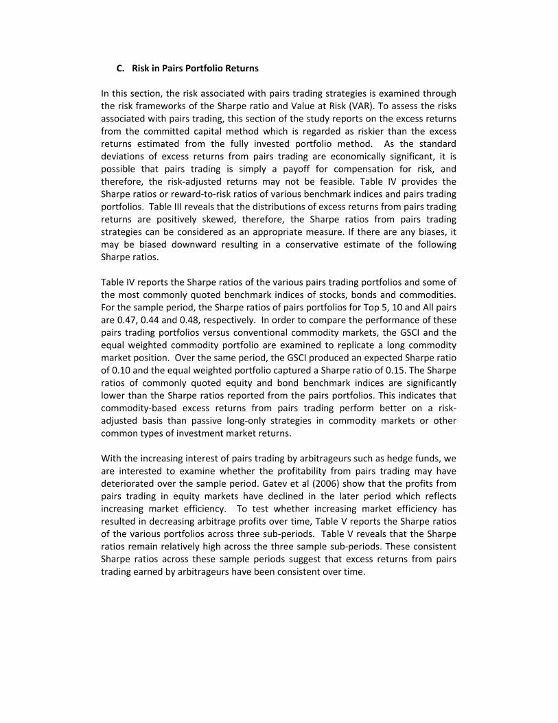
C. Risk in Pairs Portfolio Returns In this section, the risk associated with pairs trading strategies is examined through the risk frameworks of the Sharpe ratio and Value at Risk (VAR). To assess the risks associated with pairs trading, this section of the study reports on the excess returns from the committed capital method which is regarded as riskier than the excess returns estimated from the fully invested portfolio method. As the standard deviations of excess returns from pairs trading are economically significant, it is possible that pairs trading is simply a payoff for compensation for risk, and therefore, the risk‐adjusted returns may not be feasible. Table IV provides the Sharpe ratios or reward‐to‐risk ratios of various benchmark indices and pairs trading portfolios. Table III reveals that the distributions of excess returns from pairs trading returns are positively skewed, therefore, the Sharpe ratios from pairs trading strategies can be considered as an appropriate measure. If there are any biases, it may be biased downward resulting in a conservative estimate of the following Sharpe ratios. Table IV reports the Sharpe ratios of the various pairs trading portfolios and some of the most commonly quoted benchmark indices of stocks, bonds and commodities. For the sample period, the Sharpe ratios of pairs portfolios for Top 5, 10 and All pairs are 0.47, 0.44 and 0.48, respectively. In order to compare the performance of these pairs trading portfolios versus conventional commodity markets, the GSCI and the equal weighted commodity portfolio are examined to replicate a long commodity market position. Over the same period, the GSCI produced an expected Sharpe ratio of 0.10 and the equal weighted portfolio captured a Sharpe ratio of 0.15. The Sharpe ratios of commonly quoted equity and bond benchmark indices are significantly lower than the Sharpe ratios reported from the pairs portfolios. This indicates that commodity‐based excess returns from pairs trading perform better on a risk‐adjusted basis than passive long‐only strategies in commodity markets or other common types of investment market returns. With the increasing interest of pairs trading by arbitrageurs such as hedge funds, we are interested to examine whether the profitability from pairs trading may have deteriorated over the sample period. Gatev et al (2006) show that the profits from pairs trading in equity markets have declined in the later period which reflects increasing market efficiency. To test whether increasing market efficiency has resulted in decreasing arbitrage profits over time, Table V reports the Sharpe ratios of the various portfolios across three sub‐periods. Table V reveals that the Sharpe ratios remain relatively high across the three sample sub‐periods. These consistent Sharpe ratios across these sample periods suggest that excess returns from pairs trading earned by arbitrageurs have been consistent over time.

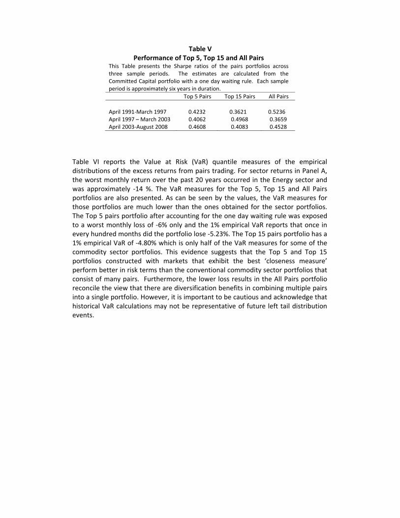
Table V Performance of Top 5, Top 15 and All Pairs

This Table presents the Sharpe ratios of the pairs portfolios across three sample periods. The estimates are calculated from the Committed Capital portfolio with a one day waiting rule. Each sample period is approximately six years in duration. Top 5 Pairs Top 15 Pairs All Pairs April 1991‐March 1997 0.4232 0.3621 0.5236 April 1997 – March 2003 0.4062 0.4968 0.3659 April 2003‐August 2008 0.4608 0.4083 0.4528

Table VI reports the Value at Risk (VaR) quantile measures of the empirical distributions of the excess returns from pairs trading. For sector returns in Panel A, the worst monthly return over the past 20 years occurred in the Energy sector and was approximately ‐14 %. The VaR measures for the Top 5, Top 15 and All Pairs portfolios are also presented. As can be seen by the values, the VaR measures for those portfolios are much lower than the ones obtained for the sector portfolios. The Top 5 pairs portfolio after accounting for the one day waiting rule was exposed to a worst monthly loss of ‐6% only and the 1% empirical VaR reports that once in every hundred months did the portfolio lose ‐5.23%. The Top 15 pairs portfolio has a 1% empirical VaR of ‐4.80% which is only half of the VaR measures for some of the commodity sector portfolios. This evidence suggests that the Top 5 and Top 15 portfolios constructed with markets that exhibit the best ‘closeness measure’ perform better in risk terms than the conventional commodity sector portfolios that consist of many pairs. Furthermore, the lower loss results in the All Pairs portfolio reconcile the view that there are diversification benefits in combining multiple pairs into a single portfolio. However, it is important to be cautious and acknowledge that historical VaR calculations may not be representative of future left tail distribution events.

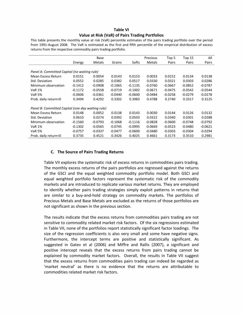
Table VI Value at Risk (VaR) of Pairs Trading Portfolios

This table presents the monthly value at risk (VaR) percentile estimates of the pairs trading portfolio over the period from 1991‐August 2008. The VaR is estimated as the first and fifth percentile of the empirical distribution of excess returns from the respective commodity pairs trading portfolio.

Energy

Base Metals Grains Softs

PreciousMetals

Top 5 Pairs

Top 15 Pairs

All Pairs

Panel A: Committed Capital (no waiting rule)Mean Excess Return 0.0151 0.0054 0.0143 0.0153 0.0033 0.0152 0.0134 0.0138Std. Deviation 0.0552 0.0285 0.0382 0.0517 0.0330 0.0321 0.0303 0.0286Minimum observation ‐0.1412 ‐0.0908 ‐0.1065 ‐0.1135 ‐0.0760 ‐0.0667 ‐0.0852 ‐0.0787VaR 1% ‐0.1172 ‐0.0558 ‐0.0719 ‐0.1002 ‐0.0671 ‐0.0475 ‐0.0542 ‐0.0544VaR 5% ‐0.0606 ‐0.0361 ‐0.0440 ‐0.0600 ‐0.0484 ‐0.0258 ‐0.0279 ‐0.0278Prob. daily return<0 0.3494 0.4292 0.3302 0.3983 0.4788 0.2740 0.3317 0.3125 Panel B: Committed Capital (one day waiting rule)Mean Excess Return 0.0148 0.0052 0.0138 0.0143 0.0030 0.0144 0.0126 0.0132Std. Deviation 0.0610 0.0274 0.0392 0.0503 0.0322 0.0340 0.0301 0.0288Minimum observation ‐0.1560 ‐0.0793 ‐0.1068 ‐0.1116 ‐0.0828 ‐0.0600 ‐0.0748 ‐0.0792VaR 1% ‐0.1302 ‐0.0565 ‐0.0745 ‐0.0995 ‐0.0669 ‐0.0523 ‐0.0480 ‐0.0621VaR 5% ‐0.0757 ‐0.0337 ‐0.0477 ‐0.0600 ‐0.0480 ‐0.0303 ‐0.0304 ‐0.0294Prob. daily return<0 0.3735 0.4521 0.3426 0.4025 0.4661 0.3173 0.3510 0.2981

C. The Source of Pairs Trading Returns

Table VII explores the systematic risk of excess returns in commodities pairs trading. The monthly excess returns of the pairs portfolios are regressed against the returns of the GSCI and the equal weighted commodity portfolio model. Both GSCI and equal weighted portfolio factors represent the systematic risk of the commodity markets and are introduced to replicate various market returns. They are employed to identify whether pairs trading strategies simply exploit patterns in returns that are similar to a buy‐and‐hold strategy on commodity markets. The portfolios of Precious Metals and Base Metals are excluded as the returns of those portfolios are not significant as shown in the previous section. The results indicate that the excess returns from commodities pairs trading are not sensitive to commodity related market risk factors. Of the six regressions estimated in Table VII, none of the portfolios report statistically significant factor loadings. The size of the regression coefficients is also very small and some have negative signs. Furthermore, the intercept terms are positive and statistically significant. As suggested in Gatev et al (2006) and Miffre and Rallis (2007), a significant and positive intercept reveals that the excess returns from pairs trading cannot be explained by commodity market factors. Overall, the results in Table VII suggest that the excess returns from commodities pairs trading can indeed be regarded as ‘market neutral’ as there is no evidence that the returns are attributable to commodities related market risk factors.

Table VII Systematic Risk of Pairs Trading Excess Returns

This table presents the regression estimates calculated from monthly excess returns constructed by the committed capital portfolio method with the one day waiting rule. The two independent variables are the GSCI Total Return Index (GSCI) and the equal weighted portfolio comprised of markets in that respective commodity sector. Excess returns are employed in these regressions estimates. The t‐statistics are calculated using the Newey and West (1987) standard errors with a four period lag correction. * and ** denote statistical significance at the 5% and 1% levels, respectively. Energy Grains Softs Top 5 Top 15 All Pairs Intercept 0.0168 0.0139 0.0147 0.0123 0.0130 0.0137t‐statistic 4.1491** 7.1775** 4.4778** 5.0297** 6.2070** 7.1866**

GSCI)(β ‐0.1329 0.0611 ‐0.1449 0.1159 0.1112 ‐0.0200

t‐statistic ‐1.6410 0.8921 ‐1.8667 1.8514 1.4788 ‐0.2710

EWP)(β 0.0689 ‐0.1194 ‐0.0260 ‐0.0845 ‐0.1293 ‐0.0676

t‐statistic 0.0573 ‐1.9210 ‐0.3183 ‐1.0525 ‐1.2451 ‐0.0858

Table VIIIRegressions Estimates with the Contrarian Model

This table presents the regression estimates calculated from monthly excess returns constructed by the committed capital portfolio method with the one day waiting rule. The independent variable in these regressions is the contrarian factor which is constructed using a three year contrarian strategy . The returns of the contrarian model are constructed by ranking the best and worst markets in each portfolio over a 36 month formation period. The portfolio then goes long the loser portfolio and goes short the winner portfolio based on the portfolio weighting scheme in Lo and MacKinlay (1990). The rollover method is employed whereby the contrarian portfolio is held and traded for one month only and then a new contrarian portfolio is formed for the subsequent month. Excess returns are employed in these regression estimates. The t‐statistics are calculated using the Newey and West (1987) standard errors with a four period lag correction. * and ** denote statistical significance at the 5% and 1% levels, respectively. Energy Grains Softs Top 5 Top 15 All Pairs Intercept 0.0131 0.0098 0.0112 0.0128 0.0109 0.0114 t‐statistic 3.2821** 4.5692** 3.1263** 5.1424* 4.8074** 6.7265**

)Contrarian(β 0.1621 0.2930 0.1934 0.1252 0.1190 0.1494

t‐statistic 2.5292* 5.9202** 5.4006** 4.7694** 3.3956** 3.8620**

D. Does Overreaction Explain Pairs Trading? We now examine whether the excess returns from pairs trading are attributable to conventional contrarian investment based strategies. This analysis is important because it allows us to ascertain whether pairs trading simply reflects compensation for contrarian investment strategies or whether the excess returns are earned by arbitrageurs who enforce the LOP. Table VIII reports the regression results of pairs trading returns and a conventional contrarian risk factor. As pairs trading strategies buy the short‐term loser and sell the short‐term winner, it is expected that the sign of the contrarian factor coefficient will be positive. Again, the portfolios of Precious Metals and Base Metals are excluded as the returns of those portfolios are not strong as shown in the previous sections. Table VIII shows that the factor loadings for the contrarian model returns exhibit the expected positive sign. All of the t‐statistics appear to be statistically significant. However, when examining the magnitude of the factor loadings, the regression coefficients are small except for the Grains sector which is relatively large compared to the other estimates. The factor loadings of the Top 5, Top 15 and All Pairs portfolios are between 0.1190 and 0.2930. Given that pairs trading executes in a similar fashion to contrarian strategies (ie. they buy the short‐term loser and sell the short‐term winner), it is expected that their returns may be related to some extent. However the regression estimates are small and not economically significant and imply that the profitability of pairs trading is unique and significantly different from contrarian strategies. This view is reinforced by the statistically significant intercept terms. The finding from Table VIII supports the view of Gatev et al (2006) that the temporal variation in return captured by pairs trading is different from what contrarian investment strategies attempt to capture. Furthermore, the intercept term of all the regressions are very large and statistically significant which indicates that the contrarian strategy provides a partial explanation only of the excess returns generated from pairs trading.

Conclusion

This study finds that pairs trading in commodity futures markets earns statistically significant excess returns. The average excess returns during the past eighteen years have been earned even after the adjustment for transaction costs. These findings are consistent with the earlier results of pairs trading in stocks in Gatev et al (2006). This study also reveals that the excess returns of pairs trading in commodities are not significantly related to the systematic risk of commodity market related returns. Hence, the pairs trading strategies in commodities are considered to be market neutral. Furthermore, the returns of pairs trading strategies are proven to be significantly different from contrarian based strategies.

The discovery of pairs trading profits in commodity futures complements the earlier findings from Gatev et al (2006) of pairs trading profits in stocks. This study on commodity futures pairs trading supports the notion from Gatev et al (2006) that these excess returns from the trading of similarly related markets is a result of arbitrageurs earning compensation for enforcing the LOP. The role of arbitrageurs in pairs trading is to act as agents who restore LOP and market efficiency. It is important to acknowledge that the excess returns from pairs trading earned by arbitrageurs are not risk‐free as they must sustain risks in order to earn these arbitrage profits. These risks associated with pairs trading can be attributed to the limits of arbitrage that confront arbitrageurs when enforcing the LOP.

References

Bodie, Z. and Rosansky, V., 1980. Risk and Return in Commodities Futures. Financial Theory, Exotic Options, and Hedging Applications.

Booth, G. G. and Ciner, C., 2001, Linkages among agricultural commodity futures

prices: evidence from Tokyo, Applied Economics Letters 8, 311‐313. DeBondt, W.F.M. and Thaler, R., 1985. Does the stock market overreact. Journal of

Finance, 40(3), 793–805. Erb, C.B. and Harvey, C.R., 2006. The Strategic and Tactical Value of Commodity

Futures. Financial Analyst Journal, 62(2), 69–99. Fama, E.F. and French, K.R., 1987. Commodity Futures Prices: Some Evidence on

Forecast Power, Premiums, and the Theory of Storage. Journal of Business, 60(1), 55 –73.

Gatev, E., Goetzmann, W.N. and Rouwenhorst, K.G., 2006. Pairs Trading:

Performance of a Relative‐Value Arbitrage Rule. Review of Financial Studies, 19(3), 797–827.

Gorton, G. and Rouwenhorst, K.G., 2006. Facts and Fantasies about Commodity

Futures. Financial Analysts Journal, 62(2), 47–68. Jegadeesh, N., 1990. Evidence of Predictable Behavior of Security Returns. Journal of

Finance, 45(3), 881–898. Karbuz, S. and Jumah, A., 1995, Cointegration and Commodity Arbitrage,

Agribusiness 11(3), 235‐243. Lamont, O.A. and Thaler, R.H., 2003. Anomalies: The Law of One Price in Financial

Markets. The Journal of Economic Perspectives, 17(4), 191–202. Lo, A. and Mackinlay, C., 1990b, When Are Contrarian Profits Due to Market

Inefficiency? Review of Financial Studies, 3(1), 175–205. Miffre, J. and Rallis, G., 2007. Momentum strategies in commodity futures markets.

Journal of Banking & Finance, 31(6), 1863–1886. Pindyck, R.S. and Rotemberg, J. J., 1990, The Excess Co‐Movement of Commodity

Prices, The Economic Journal 100(403), Dec, 1173‐1189. Shleifer, A. and Vishny, R.W., 1997. The Limits of Arbitrage. Journal of Finance, 52(1),

35–56.

von Hagen, J., 1989, Relative Commodity Prices and Cointegration, Journal of Business and Economic Statistics 7(4), Oct, 497‐503.

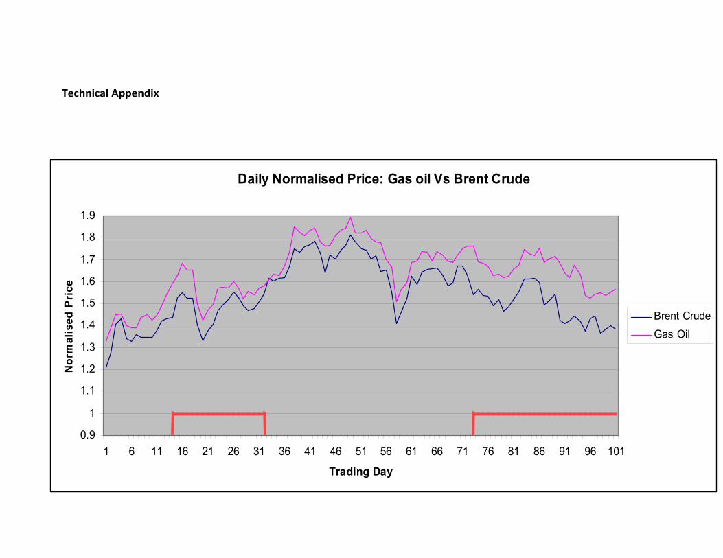
Daily Normalised Price: Gas oil Vs Brent Crude

0.9

1

1.1

1.2

1.3

1.4

1.5

1.6

1.7

1.8

1.9

1 6 11 16 21 26 31 36 41 46 51 56 61 66 71 76 81 86 91 96 101

Trading Day

Norm

alis

ed P

rice

Brent CrudeGas Oil

Technical Appendix