Testing Product Lines of Industrial Size: Advancements in ...

© Martin Fagereng Johansen, 2013 Series of dissertations submitted to the Faculty of Mathematics and Natural Sciences, University of Oslo No. 1392 ISSN 1501-7710 All rights reserved. No part of this publication may be reproduced or transmitted, in any form or by any means, without permission. Cover: Inger Sandved Anfinsen. Printed in Norway: AIT Oslo AS. Produced in co-operation with Akademika Publishing. The thesis is produced by Akademika Publishing merely in connection with the thesis defence. Kindly direct all inquiries regarding the thesis to the copyright holder or the unit which grants the doctorate.

Contents

Abstract ix

Acknowledgments xi

List of Original Publications xiii

I Overview 1

1 Introduction 31.1 Contributions . . . . . . . . . . . . . . . . . . . . . . . . . . . . . . . . . . . 4

1.2 Overview of the Industrial Cases . . . . . . . . . . . . . . . . . . . . . . . . . 6

1.2.1 The Eclipse IDEs . . . . . . . . . . . . . . . . . . . . . . . . . . . . . 6

1.2.2 TOMRA’s Reverse Vending Machines (RVMs) . . . . . . . . . . . . . 8

1.2.3 ABB’s Safety Modules . . . . . . . . . . . . . . . . . . . . . . . . . . 8

1.2.4 Finale’s Financial Reporting Systems . . . . . . . . . . . . . . . . . . 9

1.2.5 Additional Studies . . . . . . . . . . . . . . . . . . . . . . . . . . . . 9

1.3 Structure of the Thesis . . . . . . . . . . . . . . . . . . . . . . . . . . . . . . 9

2 Background and Related Work 112.1 Background: Product Line Engineering . . . . . . . . . . . . . . . . . . . . . 11

2.1.1 Feature Models . . . . . . . . . . . . . . . . . . . . . . . . . . . . . . 11

Basic Feature Models . . . . . . . . . . . . . . . . . . . . . . . . . . . 12

2.1.2 Approaches to Product Line Engineering . . . . . . . . . . . . . . . . 13

Preprocessors . . . . . . . . . . . . . . . . . . . . . . . . . . . . . . . 13

Feature-Oriented Programming . . . . . . . . . . . . . . . . . . . . . 14

Components, Frameworks and Plug-ins . . . . . . . . . . . . . . . . . 14

Orthogonal Variability Modeling (OVM) . . . . . . . . . . . . . . . . 14

Common Variability Language (CVL) . . . . . . . . . . . . . . . . . . 15

Delta-Oriented Programming . . . . . . . . . . . . . . . . . . . . . . . 18

Delta Modeling . . . . . . . . . . . . . . . . . . . . . . . . . . . . . . 18

Aspect-Oriented Programming . . . . . . . . . . . . . . . . . . . . . . 19

2.2 Background: Testing . . . . . . . . . . . . . . . . . . . . . . . . . . . . . . . 20

2.2.1 The Test Process . . . . . . . . . . . . . . . . . . . . . . . . . . . . . 20

2.2.2 V-Model . . . . . . . . . . . . . . . . . . . . . . . . . . . . . . . . . 21

2.2.3 Unit Testing . . . . . . . . . . . . . . . . . . . . . . . . . . . . . . . . 21

iii

2.2.4 Model-based Testing . . . . . . . . . . . . . . . . . . . . . . . . . . . 21

2.2.5 Regression Testing . . . . . . . . . . . . . . . . . . . . . . . . . . . . 22

2.2.6 Category Partition (CP) . . . . . . . . . . . . . . . . . . . . . . . . . . 23

2.3 Related Work: Product Line Testing . . . . . . . . . . . . . . . . . . . . . . . 23

2.3.1 Overview . . . . . . . . . . . . . . . . . . . . . . . . . . . . . . . . . 23

Contra-SPL-philosophies . . . . . . . . . . . . . . . . . . . . . . . . . 24

Reusable Component Testing . . . . . . . . . . . . . . . . . . . . . . 24

Feature Interaction . . . . . . . . . . . . . . . . . . . . . . . . . . . . 24

Model-based SPL Testing . . . . . . . . . . . . . . . . . . . . . . . . 25

Reuse . . . . . . . . . . . . . . . . . . . . . . . . . . . . . . . . . . . 26

Subset-Heuristics . . . . . . . . . . . . . . . . . . . . . . . . . . . . . 27

2.3.2 Product Line Use case Test Optimization (PLUTO) . . . . . . . . . . . 28

Product Line Use Cases (PLUCs) . . . . . . . . . . . . . . . . . . . . 28

Using CP on PLUCs . . . . . . . . . . . . . . . . . . . . . . . . . . . 28

2.3.3 Scenario-based Test Case Derivation (ScenTED) . . . . . . . . . . . . 30

2.3.4 Combinatorial Interaction Testing (CIT) . . . . . . . . . . . . . . . . . 31

Covering Arrays . . . . . . . . . . . . . . . . . . . . . . . . . . . . . 33

2.3.5 Customizable Activity Diagrams, Decision Tables, ... (CADeT) . . . . 34

2.3.6 Model-driven Software Product Line Testing (MoSo-PoLiTe) . . . . . 35

2.3.7 Incremental Testing . . . . . . . . . . . . . . . . . . . . . . . . . . . . 36

2.4 Related Work: Algorithms for Covering Array Generation . . . . . . . . . . . 38

2.4.1 IPOG . . . . . . . . . . . . . . . . . . . . . . . . . . . . . . . . . . . 39

2.4.2 MoSo-PoLiTe . . . . . . . . . . . . . . . . . . . . . . . . . . . . . . . 41

2.4.3 CASA . . . . . . . . . . . . . . . . . . . . . . . . . . . . . . . . . . . 43

2.4.4 Other Algorithms . . . . . . . . . . . . . . . . . . . . . . . . . . . . . 46

3 Contributions 493.1 Overview and Relation to the State of the Art . . . . . . . . . . . . . . . . . . 49

3.2 Generation of Covering Arrays from Large Feature Models . . . . . . . . . . . 50

3.2.1 Difficulty of Covering Array Generation . . . . . . . . . . . . . . . . . 50

SPLE-SAT is Easy . . . . . . . . . . . . . . . . . . . . . . . . . . . . 50

Covering Array Generation is Feasible . . . . . . . . . . . . . . . . . . 52

3.2.2 Scalable t-wise Covering Array Generation . . . . . . . . . . . . . . . 52

3.2.3 Consolidations . . . . . . . . . . . . . . . . . . . . . . . . . . . . . . 53

3.3 Optimized Testing in the Presence of Homogeneous Abstraction Layers . . . . 54

3.3.1 Description of the Technique . . . . . . . . . . . . . . . . . . . . . . . 54

3.3.2 Application to Finale’s Systems . . . . . . . . . . . . . . . . . . . . . 55

3.3.3 Application to the Eclipse IDEs . . . . . . . . . . . . . . . . . . . . . 55

3.4 Market-Focused Testing based on Weighted Sub-Product line Models . . . . . 56

3.4.1 Weighted Sub-Product Line Models . . . . . . . . . . . . . . . . . . . 56

3.4.2 Algorithms Based on These Models . . . . . . . . . . . . . . . . . . . 57

Weighted t-sets . . . . . . . . . . . . . . . . . . . . . . . . . . . . . . 57

Weighted Covering Array Generation . . . . . . . . . . . . . . . . . . 57

Weight Coverage . . . . . . . . . . . . . . . . . . . . . . . . . . . . . 57

iv

Incremental Evolution . . . . . . . . . . . . . . . . . . . . . . . . . . 57

3.4.3 Application to TOMRA’s RVMs . . . . . . . . . . . . . . . . . . . . . 58


3.5 Agile and Automatic Software Product Line Testing . . . . . . . . . . . . . . . 59

3.5.1 Challenges in Need of an Answer . . . . . . . . . . . . . . . . . . . . 59

3.5.2 Testing Interactions using Tests for Features . . . . . . . . . . . . . . . 60

3.5.3 Evaluation of Previous Techniques . . . . . . . . . . . . . . . . . . . . 60

Reusable Component Testing – Pros and Cons . . . . . . . . . . . . . 60

Combinatorial Interaction Testing – Pros and Cons . . . . . . . . . . . 61

3.5.4 The Automatic CIT Technique . . . . . . . . . . . . . . . . . . . . . . 61


3.5.6 Application to ABB’s Safety Modules . . . . . . . . . . . . . . . . . . 62

3.6 Tool Support and Integration of Achievements . . . . . . . . . . . . . . . . . . 65

4 Discussion 674.1 Limitations and Threats to Validity . . . . . . . . . . . . . . . . . . . . . . . . 67

4.2 Future Work . . . . . . . . . . . . . . . . . . . . . . . . . . . . . . . . . . . . 70

4.2.1 Empirical Investigations . . . . . . . . . . . . . . . . . . . . . . . . . 70

4.2.2 Complex Product Lines . . . . . . . . . . . . . . . . . . . . . . . . . . 70

Mixed Hardware and Software Product Lines . . . . . . . . . . . . . . 71

Mixed-Variability Systems . . . . . . . . . . . . . . . . . . . . . . . . 71

High Commonality, Few Products . . . . . . . . . . . . . . . . . . . . 71

Optimized Distribution of Test Cases . . . . . . . . . . . . . . . . . . 72

4.2.3 Product Line Engineering . . . . . . . . . . . . . . . . . . . . . . . . 72

Distributed Variability Specifications . . . . . . . . . . . . . . . . . . 72

Utilizing Implementation Information . . . . . . . . . . . . . . . . . . 72

Design Principles and SPL Testing . . . . . . . . . . . . . . . . . . . . 73

Exploiting Version Information . . . . . . . . . . . . . . . . . . . . . 73

4.2.4 Algorithms . . . . . . . . . . . . . . . . . . . . . . . . . . . . . . . . 73

Further Improvements of ICPL . . . . . . . . . . . . . . . . . . . . . . 73

Upper bound for ICPL . . . . . . . . . . . . . . . . . . . . . . . . . . 74

Extracting Basic Feature Models . . . . . . . . . . . . . . . . . . . . . 74

Evolving Covering Arrays . . . . . . . . . . . . . . . . . . . . . . . . 74

4.2.5 Engineering . . . . . . . . . . . . . . . . . . . . . . . . . . . . . . . . 75

Using Virtual Machines . . . . . . . . . . . . . . . . . . . . . . . . . 75

Full Testing of the Eclipse IDEs . . . . . . . . . . . . . . . . . . . . . 75

5 Conclusion 775.1 Results . . . . . . . . . . . . . . . . . . . . . . . . . . . . . . . . . . . . . . . 77

5.2 Evaluation . . . . . . . . . . . . . . . . . . . . . . . . . . . . . . . . . . . . . 78

Bibliography 81

v

II Research Papers 95

6 Overview of Research Papers 97

7 Paper 1: Properties of Realistic Feature Models Make Combinatorial Testing ofProduct Lines Feasible 101Background . . . . . . . . . . . . . . . . . . . . . . . . . . . . . . . . . . . . . . . 104

The Case for Tractable t-wise Covering Array Generation . . . . . . . . . . . . . . . 107

Performance of Chvátal’s Algorithm for Covering Array Generation . . . . . . . . . 109

Discussion . . . . . . . . . . . . . . . . . . . . . . . . . . . . . . . . . . . . . . . . 114

8 Paper 2: An Algorithm for Generating t-wise Covering Arrays from Large FeatureModels 119Background and Related Work . . . . . . . . . . . . . . . . . . . . . . . . . . . . . 122

The Basic Algorithm . . . . . . . . . . . . . . . . . . . . . . . . . . . . . . . . . . 123

The New Algorithm: ICPL . . . . . . . . . . . . . . . . . . . . . . . . . . . . . . . 124

Results and Comparison . . . . . . . . . . . . . . . . . . . . . . . . . . . . . . . . 126

Threats to Validity . . . . . . . . . . . . . . . . . . . . . . . . . . . . . . . . . . . . 129

Future Work . . . . . . . . . . . . . . . . . . . . . . . . . . . . . . . . . . . . . . . 129

9 Paper 3: Bow Tie Testing: A Testing Pattern for Product Lines 131Background and Motivating Example . . . . . . . . . . . . . . . . . . . . . . . . . 134

The Bow Tie Structure . . . . . . . . . . . . . . . . . . . . . . . . . . . . . . . . . 136

Pattern: Bow Tie Testing . . . . . . . . . . . . . . . . . . . . . . . . . . . . . . . . 137

Restructuring to Enable the Application of the Pattern . . . . . . . . . . . . . . . . . 142

Similar Patterns . . . . . . . . . . . . . . . . . . . . . . . . . . . . . . . . . . . . . 143

10 Paper 4: Generating Better Partial Covering Arrays by Modeling Weights on Sub-Product Lines 147Background and Related Work . . . . . . . . . . . . . . . . . . . . . . . . . . . . . 151

Weighted Combinatorial Interaction Testing . . . . . . . . . . . . . . . . . . . . . . 154

Industrial Application: TOMRA . . . . . . . . . . . . . . . . . . . . . . . . . . . . 157

Applicability to the Eclipse IDEs . . . . . . . . . . . . . . . . . . . . . . . . . . . . 162

11 Paper 5: A Technique for Agile and Automatic Interaction Testing for ProductLines 165Background and Related Work . . . . . . . . . . . . . . . . . . . . . . . . . . . . . 168

Proposed Technique . . . . . . . . . . . . . . . . . . . . . . . . . . . . . . . . . . . 171

Evaluation with Two Applications and Results . . . . . . . . . . . . . . . . . . . . . 174

Benefits and Limitations . . . . . . . . . . . . . . . . . . . . . . . . . . . . . . . . 179

III Appendices 183

A Resource Pages for Papers 185Resource Page for Paper 1 . . . . . . . . . . . . . . . . . . . . . . . . . . . . . . . 186

vi

Resource Page for Paper 2 . . . . . . . . . . . . . . . . . . . . . . . . . . . . . . . 188




B Algorithms Based on Weighted Sub-Product Line Models 201B.1 Some New Terms . . . . . . . . . . . . . . . . . . . . . . . . . . . . . . . . . 201

B.2 Calculating Weights . . . . . . . . . . . . . . . . . . . . . . . . . . . . . . . . 201

B.3 Generating a Weighted Covering Array . . . . . . . . . . . . . . . . . . . . . 203

B.4 Generating Improvement Suggestions . . . . . . . . . . . . . . . . . . . . . . 204

C Details for Comparisons 207

D Technical About the Tools 211D.1 Version History . . . . . . . . . . . . . . . . . . . . . . . . . . . . . . . . . . 211

D.2 Architecture . . . . . . . . . . . . . . . . . . . . . . . . . . . . . . . . . . . . 211

D.2.1 Feature Model Formats . . . . . . . . . . . . . . . . . . . . . . . . . . 213

D.2.2 Configuration Set Formats . . . . . . . . . . . . . . . . . . . . . . . . 213

D.2.3 Weighted Sub-Product Line Formats . . . . . . . . . . . . . . . . . . . 214

D.2.4 Versions . . . . . . . . . . . . . . . . . . . . . . . . . . . . . . . . . . 214

D.2.5 Overview of Algorithms and Object Structures . . . . . . . . . . . . . 215

D.3 User Manual . . . . . . . . . . . . . . . . . . . . . . . . . . . . . . . . . . . . 215

D.3.1 Analysis . . . . . . . . . . . . . . . . . . . . . . . . . . . . . . . . . 216

D.3.2 Generating Covering Arrays . . . . . . . . . . . . . . . . . . . . . . . 218

D.3.3 Extending Towards a Covering Array . . . . . . . . . . . . . . . . . . 218

D.3.4 Improving a Partial Covering Array . . . . . . . . . . . . . . . . . . . 219

D.3.5 Automatic CIT: Eclipse-Based Product Lines . . . . . . . . . . . . . . 220

D.3.6 Automatic CIT: CVL Based Product Lines . . . . . . . . . . . . . . . 222

E Details on the Eclipse Case Study 223E.1 Technical About Eclipse v3.7.0 (Indigo) . . . . . . . . . . . . . . . . . . . . . 223

E.2 Contributed Artifacts . . . . . . . . . . . . . . . . . . . . . . . . . . . . . . . 225

E.3 Details on Automatic CIT of Eclipse . . . . . . . . . . . . . . . . . . . . . . . 225

E.3.1 Feature Models and Covering Arrays . . . . . . . . . . . . . . . . . . 227

E.3.2 Implementation with the Eclipse Platform’s Plug-in System . . . . . . 228

E.3.3 Bindings Between Feature Names and System Artifacts . . . . . . . . 229

E.3.4 Automatic Building . . . . . . . . . . . . . . . . . . . . . . . . . . . . 229

E.3.5 Bindings Between Feature Names and Test Suites . . . . . . . . . . . . 230

vii

Abstract

Due to varying demands by customers, some software systems need to be configurable and

need to have optional features. Customers then configure their system according to their special

needs and select the features they need. A problem the developers of such systems face is the

possibility of latent faults awakened by some of its set-ups. A system used by thousands, if not

by millions, cannot fail for many before it becomes a major problem for the developers. Indeed,

if many systems fail, the general view of the quality of the system might be beyond repair. For

example, the Eclipse IDEs are popular software systems; they are also highly customizable.

There are probably tens of thousands of unique set-ups of the Eclipse IDEs in use.

This is one example of product line development, and the field that studies the construction

and development of product lines is product line engineering. One way of gaining confidence in

the quality of a product line—and any set-ups of it—is through testing. Product line testing, the

strategic exercising of the product line in order to gain confidence in the quality of the product

line and any configuration of it, is the subject of this thesis.

The strategy followed today with documented results is reusable component testing, the

testing of the product line’s common parts in isolation: If a common part fails in isolation

because of an internal fault, it will likely cause failures in any product of which it is a part.

Testing something in isolation will not, naturally, rule out interaction faults between these parts.

Combinatorial interaction testing (CIT) can test interactions and is—as of today—the tech-

nique closest to being realistically applicable in industrial settings. This technique is the starting

point of the contributions of this thesis. CIT starts by sampling some products of the product

line. The products are selected such that all combinations of a few features are in at least one

of the products. This selection criterion is such that faults are more likely to show up in these

products than in randomly selected products. As executable systems, they can be tested.

One significant problem with CIT is the lack of an efficient algorithm for the selection of

products. The existing algorithms scale insufficiently for the larger product lines. This effec-

tively rules it out in industrial settings. A contribution of this thesis is an algorithm (called ICPL)

that can perform the selection process even for product lines of industrial size. A preliminary

analysis of the problem was a necessary prior contribution contributed before the algorithm

could be developed. These two contributions taken as a whole provides an efficient algorithm

for this one bottle-neck of the application of CIT.

Having a scalable algorithm for selection enables the efficient application of CIT. To estab-

lish and demonstrate the usefulness of CIT, three advancements of CIT with applications were

contributed.

Firstly, a common situation with product lines is portability across various hardware archi-

tectures, operating systems, database systems, etc. One construct that deals effectively with

ix

such situations is a homogeneous abstraction layer. It provides a uniform way of accessing

these differing systems. Usually, only one implementation of a homogeneous abstraction layer

can be present in a product. This deteriorates the performance of CIT. The selection criterion

used by CIT is to strategically select simple combinations of features. Only being allowed to

activate one and one feature is limiting to the algorithms. It was noticed that products differing

only in their implementation of homogeneous abstraction layers can be tested using the same

test suite. This enables a voting oracle or a gold standard oracle to be set up. This contribution

thus turns the aforementioned problem into a strength.

Secondly, the selection criterion of CIT ensures all simple interactions are exercised. In

some cases, this leads to redundant testing. A product line’s market situation might exclude

large classes of feature combinations or indicate then some combinations are more common

than others. These things can be captured in a weighted sub-product line model, which, along

with associated algorithms, is another contribution of this thesis.

Thirdly, one way to fully automate the application of CIT is to create the test cases before

testing and then strategically allocate and automatically run those test cases in each application

of CIT. Such a technique and a full application of it on the Eclipse IDEs using its existing test

cases is also a contribution of this thesis.

In summary, this thesis contributes an algorithm that enables the application of CIT in indus-

trial settings. Further, three advancements of CIT with applications were contributed to advance

and demonstrate CIT as a product line testing technique.

x

Acknowledgments

This work has been conducted as a part of the Norwegian VERDE project funded by the Re-

search Council of Norway. The Norwegian VERDE project participated in the international

VERDE project ITEA 2 - ip8020. The international VERDE is a project within the ITEA 2 -

Eureka framework.

First of all, I would like to thank my two supervisors Øystein Haugen and Franck Fleurey;

they were naturally the closest cooperators during my PhD work on all issues. They provided

me with the guidance I needed to get safely through this process, they were always available to

answer my questions and for a good discussion. I could not have done it without their valuable

guidance.

I have during the PhD studies been employed by SINTEF ICT as a research fellow at the ini-

tially named Department of Cooperative and Trusted Systems later renamed to the Department

of Networked Systems and Services. I owe my thanks to the research director Bjørn Skjellaug

and all the colleagues for providing a very pleasant and motivating work environment.

I would like to thank Anders Emil Olsen who, while working for TOMRA, introduced me

and SINTEF to a highly interesting industrial case, the testing of TOMRA’s reverse vending

machines; it was not initially a part of the Norwegian VERDE project. It was a great experience

working together with TOMRA Verilab’s Anne Grete Eldegaard and Thorbjørn Syversen on

this case study.

I also had the great opportunity to work together with Frank Mikalsen from Finale Systems

on the Finale case study, and primarily Erik Carlson, Jan Endresen and TormodWien from ABB

Corporate Research on the ABB case studies.

The VERDE project provided me with everything I wanted from a PhD. I got a firsthand

experience with both the national and international research communities, and I got the first-

hand experience of working together with people from three interesting companies on their

industrial cases. Each gave me invaluable experience and provided a great start of a research

career.

Last but not the least, I would like to thank my girlfriend Hilde Galleberg Johnsen for her

continuous support on all matters during the years of my PhD work.

xi

List of Original Publications

1. Martin Fagereng Johansen, Øystein Haugen, and Franck Fleurey, "Properties of Realistic

Feature Models Make Combinatorial Testing of Product Lines Feasible," Model DrivenEngineering Languages and Systems – 14th International Conference, MODELS 2011,Wellington, New Zealand, October 16–21, 2011. Proceedings, Springer, 2011, p. 638.

2. Martin Fagereng Johansen, Øystein Haugen, and Franck Fleurey, "An Algorithm for Gen-

erating t-wise Covering Arrays from Large Feature Models," Software Product Lines –16th International Conference, SPLC 2012, Salvador, Brazil, September 2–7, 2012. Pro-ceedings – Volume 1, ACM, 2012, p. 46.

3. Martin Fagereng Johansen, Øystein Haugen, and Franck Fleurey, "Bow Tie Testing –

A Testing Pattern for Product Lines," Pattern Languages of Programs – 16th EuropeanConference, Proceedings, ACM, 2012, p. 9:1.

4. Martin Fagereng Johansen, Øystein Haugen, Franck Fleurey, Anne Grete Eldegard, and

Torbjørn Syversen, "Generating Better Partial Covering Arrays by Modeling Weights on

Sub-Product Lines," Model Driven Engineering Languages and Systems – 15th Interna-tional Conference, MODELS 2012, Innsbruck, Austria, September 30–October 5, 2012.Proceedings, Springer, 2012, p. 269.

5. Martin Fagereng Johansen, Øystein Haugen, Franck Fleurey, Erik Carlson, Jan Endresen,

and TormodWien, "A Technique for Agile and Automatic Interaction Testing for Product

Lines," Testing Software and Systems – 24th IFIP International Conference, ICTSS ’12,Aalborg, Denmark, November 19–21, 2012. Proceedings, Springer, 2012, p. 39.

xiii

Part I

Overview

1

Chapter 1

Introduction

“one element in the price of everyarticle is the cost of its verification.”

– Charles Babbage

One size does not always fit all; or one software system does not always fit all users. There are

many situations, however, where they almost fit all. In these cases it might be better to make

a configurable system, instead of several single systems. Indeed, the cost of single systems

can be decreased, and the efficiency of developing them can be greatly increased by making a

configurable system.

A company that produces, for example, t-shirts need to produce them of varying sizes for

obvious reasons, or with a varying color or motives. Still, much of the production of these

t-shirts is similar: They can use the same fabric, they can be dyed similarly and their motives

applied with the same equipment. This is surely more efficient than having a separate production

process for each kind of t-shirt.

A similar example could easily be mentioned for cars.

Historically, when products are offered in this manner, they were offered lined up, the cus-

tomer browsing the products to find one that specifically suits his or her needs; thus, the term

product line.These notions were brought into software engineering; thus, the term software product lines.

Their development has been studied in the field of software product line engineering (SPLE).

To continue the t-shirt analogy, because t-shirts of various sizes, colors and motives are

made from the same fabric, dyes and motives, no one would be surprised to learn that several

t-shirts made with the same quality fabric all are of good quality with respect to the fabric. This

commonality, once verified, gives us a lot of information about the quality of the completed

t-shirts. In the same way, a wrongly mixed dye might cause all t-shirts colored with it to drasti-

cally fade when washed. Washing one t-shirt of each dye will give us a lot of information about

the other t-shirts colored with the same dyes.

The same analogy holds for software, but just how to gain confidence in the quality of any

product of a product line, remains an open question. How to use testing for quality assurance

of software product lines is the general problem of this thesis.

Testing the common parts out of which products are composed is already an established

practice. As with the t-shirts, this gives us some level of confidence in the composed products.

3

It does not, however, tell us about the interaction between the parts. Various techniques are

being researched to achieve this goal. Among the suggested techniques, this thesis advances

one particular technique, combinatorial interaction testing. This technique is to select a small

set of products such that each combination of t options (typically 1, 2 or 3) occurs in at least one

of the products. For the t-shirts, it would mean producing t-shirts such that ever combination of,

for example, 2 features are in at least one t-shirt: every combination of color and motif, every

combination of motif and size, etc. These products are called the t-wise products. The t-wise

criterion ensures that interaction faults are significantly more likely to occur in these selected

products than in the same number of randomly selected products.

Counter-intuitively, this t-wise selection process is computationally expensive. It has even

been argued that the selection is so difficult that it will remain infeasible for practical purposes.

It is thus a bottle-neck in the application of combinatorial interaction testing. Contribution 1

and 2 of this thesis culminates in an algorithm that performs this selection efficiently enough to

make combinatorial interaction testing usable in practice.

Having resolved this bottle-neck, the utilization of combinatorial interaction testing in in-

dustrial settings still requires issues to be addressed. The existence of a scalable means of

selecting the products to test, however, opens up for and encourages further developments of

the technique. Three such developments are the further contributions of this thesis.

1.1 Contributions

The main contributions of this thesis all relate to the testing of product lines using combinatorial

interaction testing (CIT). Figure 1.1 shows the CIT testing process with the five contributions

of this thesis marked as 1–5. The general technique of using CIT to test product lines has been

studied for some time [42]. It starts with three assets, two of which are ubiquitous in software

projects: Asset B is the implementation of a software system, and Asset C is test cases for

this system. Asset A is the specification of variability in the system. Software product line

engineering recommends maintaining a feature diagram, Asset A; however, this is not required

to maintain a product line. The act of configuring and building a system can be done manually

by domain experts using tooling not built on product line concepts. This was the case for all our

four industrial case studies. However, making a feature diagram (and the bindings) is neither

hard nor time consuming; it was done for all four case studies.

When Asset A–C are available, CIT can be carried out as follows: Configurations can be

sampled from the feature diagram; Asset D shows the sampled configurations out of the swarm

of possible configurations. Now, given the small number of selected configurations, it is feasible

to build all their corresponding products; the configurations are applied to the implementation

assets to produce a small number of actual, runnable products, Asset E, products P1–4. These

runnable products can then be tested using the test cases, Asset C, to produce a test report, Asset

F. Thus, with CIT, we start with the implementation and end up with a report on its quality.

The five papers, on which this thesis is based, present results that contribute to this process.

Their points of contribution are marked as 1–5 respectively on Figure 1.1.

Contributions 1, 2, 4) The contributions of Paper 1 [78], 2 [79] and 4 [82] all relate to the

sampling of configurations for testing purposes. The sampling stage was, prior to the contribu-

4

Figure 1.1: Contributions 1, 2, 3, 4 and 5 as Parts of a Whole Test Process

tions of this thesis, considered too computationally expensive to be done in industrial settings.

Indeed, no scalable algorithm or tool existed. The primary contribution of Paper 1 is an argu-

ment for why this stage is feasible in practice: Providing a single valid configuration of a feature

diagram is classified as NP-hard; however, having a product line without any products does not

make sense in practice. Thus, it is argued that realistic feature diagrams are easily configurable,

something that is backed up by a study of realistic feature models.

Paper 2 contributes a scalable algorithm (and tooling) for performing the sampling, thereby

consolidating the argument of Paper 1. The contributed algorithm, ICPL, was and still is the

fastest algorithm for CIT product sampling for product lines of industrial size, and the first to

be able to sample products from the largest available product lines.

Paper 4 also contributes to the sampling stage. A premise of CIT is that all possible simple

interactions must be exercised to evaluate the quality of a product line. However, depending on

the market of the product line, not all interactions can occur, or seldomly occur. A weightedsub-product line model, a type of model contributed in Paper 4, allows the market situation to be

captured. Associated algorithms, also contributed, then enable the product sampling to take the

market situation into account to sample a smaller set of more market-relevant configurations.

Contribution 3) Often, the products of a product line need to work with different imple-

mentations of what is essentially the same thing: for example, a file system, network interface

or a database system. A homogeneous abstraction layer provides a uniform interface which the

product line assets can interact with instead of having one asset for each concrete implementa-

tion. There is, then, one implementation of the interface for each supported variant; for example,

for each variant of file systems, network interfaces or database systems. Each implementation

5

of the abstraction layer is mutually exclusive. One implementation of an abstraction layer suf-

fice in these situations. This causes the number of products selected in CIT product sampling

to increase because the sampling algorithm is restricted to choosing one implementation per

product where it elsewhere can strategically select multiple features.

The contribution of Paper 3 [80] is to turn this problem into a benefit: Such homogeneous

abstraction layers enable the reuse of existing test suites across many products selected in CIT

product sampling. This step is not necessary to perform CIT; it is noted in Figure 1.1 as a

marking of the configurations sampled. Those sampled configurations that only differ in the

implementation of homogeneous abstraction layers are marked. These marks can then be uti-

lized to make a voting oracle or a gold standard oracle as a part of the "Testing" stage.

Contribution 5) The contribution of Paper 5 [81] is noted in Figure 1.1 as an arrow going

from the upper-left to the lower-right. It is a technique to fully automate the application of CIT:

Given a feature diagram with bindings to the implementation and a set of test cases, it produces

a test report in one click.

Among other things, it required an automatic allocation of the existing test cases: This was

accomplished in the "Allocating" stage of Figure 1.1 by allocating the tests for the products

sampled to those in which the test cases’ required features were present.

A large-scale application this technique was done to the part of the Eclipse IDEs supported

by the Eclipse Project. It was and still is the largest documented and reproducible application

of a fully automatic testing of a software product line of industrial size.

Tool Support) All the contributions are supported by complete implementations in SPLCA-

Tool (Software Product Line Covering Array Tool) v0.3 and v0.4 and the Automatic CIT tool

suite, all written by the authors of this thesis and freely available as open source. Technical

details and a user manual for these tools are available as Appendix D.

1.2 Overview of the Industrial Cases

We applied parts of the contributions of this thesis to three commercial, industrial cases. In

addition, we included one open source system. This was for the purpose of being able to work

with the source code, publish the results and provide reproducible experiments. This open

source case study will be described first followed by the three commercial, industrial cases.

1.2.1 The Eclipse IDEs

Eclipse is a collection of integrated development environments (IDEs) developed by the Eclipse

Project [132]. An IDE is a program in which developers work with (primarily) software. They

usually have editors especially designed to write certain programming languages. The IDE does

various analyses in the background to give the users direct feedback or help when working. The

IDE also keeps the system built at any time so that the developer can try the system they are de-

veloping with a single click. There are usually several editors open at any time, each specialized

for their language or data format, each with help and guidance. All these tools are integrated

into a complete environment for development, thereby the name integrated development envi-ronment.

6

Figure 1.2: Overview of the Eclipse Plug-in System from [51]

The Eclipse IDEs are widely used, especially among Java developers. It is a competitor to

Microsoft’s Visual Studio which is primarily used for Windows and .NET programming in C++

and C#.

Eclipse is developed openly, is open source and free. The source code repositories and bug

tracking systems used by the developers are online [51].

Eclipse is developed by, among others, Erich Gamma, the main author of the influential first

book on design patterns [52]. Figure 1.2 shows Gamma’s own overview of the design and how

variability is supported in Eclipse. The Eclipse platform exposes extension-points that plug-ins

can implement. These plug-ins can then expose new extension points, etc. Eclipse has a large

community of plug-in developers.

Eclipse is also the recipient of the 2011 ACM Software System Award.

All of this made it a prime candidate as a case study for this thesis: It is open source, all

results found can be published and documented, and the experiments can be reproduced by

other researchers.

We studied v3.7.0 (Indigo) because it was the latest release in the summer of 2011. Twelve

products were, at the release, configured by the Eclipse Project and offered for download; users

were free to configure their own version of the IDE using the built-in tools of the basic platform.

(a) Windows (b) Linux, GTK (c) Linux, Motif (d) Mac (e) Mac, Photon

Figure 1.3: The Same Eclipse-based System Running in Different Windowing Systems (From

http://www.eclipse.org/swt/, May 2011)

7

1.2.2 TOMRA’s Reverse Vending Machines (RVMs)

TOMRA’s reverse vending machines (RVMs) [156] handle the return of deposit beverage con-

tainers at retail stores such as supermarkets, convenience stores and gas stations. In Norway,

were TOMRA resides, customers are required by law to pay an amount for each container they

buy which is given back to them if they decide to return the container. In Norway, all vendors

that sell beverage containers are required by law to take them back and return the money upon

request.

Figure 1.4: Several Variants of TOMRA RVMs

Figure 1.5: Behind the Front of TOMRA RVMs

The RVMs are delivered all over the world, and the market is expanding. However, indi-

vidual market requirements and the needs of TOMRA’s customers within the different markets

can vary significantly. TOMRA’s reverse vending portfolio therefore offers a high degree of

flexibility in terms of how a specific installation is configured.

At TOMRAVerilab they are responsible for testing these machines. Their existing test setup

was a set of manually configured test products. These test products were tested using manually

written tests that were executed both automatically and manually.

1.2.3 ABB’s Safety Modules

ABB is a large international company working with power and automation technologies. One

of ABB’s divisions develops a device called a Safety Module [1].

The ABB Safety Module is a physical component that is used in, among other things, cranes,

conveyor belts and hoisting machines. Its task is to ensure safe reaction to problematic events,

8

Figure 1.6: The ABB Safety Module

such as the motor running too fast, or if a requested stop is not handled as required. It includes

various software configurations to adapt it to its particular use and safety requirements.

A simulated version of the ABB Safety Module was built—independently of the work in

this thesis—for experimenting with modeling tools and their interoperability. It is this version

of the ABB Safety Module which testing is reported in this thesis.

1.2.4 Finale’s Financial Reporting Systems

Finale Systems AS is a provider of software for financial reporting and tax returns. Their

portfolio consists of nine main products that automate many tasks or subtasks in the reporting

of accounting data to the public authorities [4]. For example, according to Finale, approximately

6,300 auditors and accountants use one of their systems to produce 130,000 annual settlements.

Their nine products defer many configuration options to users, making the number of pos-

sible configurations high. Companies use a wide range of accounting systems that Finale’s

systems need to interact with. They interact with these systems though a homogeneous ab-

straction layer. This abstraction layer is implemented concretely for each specific accounting

system.

1.2.5 Additional Studies

In addition to these four case studies, 19 realistic feature models were gathered from research

and industry; they are listed in Table 1.1. They include three large feature models extracted

from three large systems by She et al. 2011 [141]: the Linux kernel, FreeBSD and eCos. Only

the feature models of these studies were used, and they were used as is.

Four realistic feature models were made for each of our industrial case studies, but these

were not included in some experiments to remain unbiased.

These 19 feature models were used in Contribution 1, the analysis of the covering array

generation from realistic feature models, and in Contribution 2, the development of an algorithm

for covering array generation.

1.3 Structure of the Thesis

The Faculty of Mathematics and Natural Sciences at the University of Oslo recommends that a

dissertation is presented either as a monograph or as a collection of research papers. We have

chosen the latter.

9

Table 1.1: Models and Sources

System Name Model File Name Source

X86 Linux kernel 2.6.28.6 2.6.28.6-icse11.dimacs [141]

Part of FreeBSD kernel 8.0.0 freebsd-icse11.dimacs [141]

eCos 3.0 i386pc ecos-icse11.dimacs [141]

e-Shop Eshop-fm.xml [95]

Violet, graphical model editor Violet.m http://sourceforge.net/projects/violet/

Berkeley DB Berkeley.m http://www.oracle.com/us/products/database/berkeley-db/index.html

Arcade Game Maker Pedagogical Prod-

uct Line

arcade_game_pl_fm.xml http://www.sei.cmu.edu/productlines/ppl/

Graph Product Line Graph-product-line-fm.xml [103]

Graph Product Line Nr. 4 Gg4.m an extended version of the Graph

Product line from [103]

Smart home smart_home_fm.xml [165]

TightVNC Remote Desktop Software TightVNC.m http://www.tightvnc.com/AHEAD Tool Suite (ATS) Product Line Apl.m [157]

Fame DBMS fame_dbms_fm.xml http://fame-dbms.org/Connector connector_fm.xml a tutorial [163]

Simple stack data structure stack_fm.xml a tutorial [163]

Simple search engine REAL-FM-12.xml [105]

Simple movie system movies_app_fm.xml [122]

Simple aircraft aircraft_fm.xml a tutorial [163]

Simple automobile car_fm.xml [166]

The thesis is based on a collection of five research papers and is structured into two main

parts plus an appendix. Part I provides the context and an overall view of the work. Part II

contains the collection of research papers. The purpose of Part I is to explain the overall context

of the results presented in the research papers and to explain how they fit together. Part I is

organized into the following chapters:

• Chapter 1 - Introduction introduces the problem, contributions and industrial cases.

• Chapter 2 - Background and Related Work presents the relevant background and other

work related to the contributions of this thesis.

• Chapter 3 - Contributions presents an overview of the contributions and how they fit

together.

• Chapter 4 - Discussion presents threats to validity and provides ideas for future work.

• Chapter 5 - Conclusion presents the conclusions of this thesis.

Each research paper in Part II is meant to be self-contained and can be read independently of the

others. The papers therefore overlap to some extent with regard to explanations and definitions

of the basic terminology. We recommend that the papers are read in the order they appear in the

thesis.

• Chapter 6 - Overview of Research Papers is the first chapter of Part II. It provides

publication details and a summary of each research paper.

Part III contains a series of appendices. The interested readers are referred to them throughout

Part I for additional details.

10

Chapter 2

Background and Related Work

This chapter introduces the relevant background on product line engineering and testing, in

Section 2.1 and 2.2, respectively, followed by related work: First, the related work in product

line testing is presented in Section 2.3. Then, because the contributions of this thesis is based

on an efficient algorithm for t-wise covering array generation (called ICPL), other algorithms

for the same problem are presented, discussed and related to it in detail in Section 2.4.

2.1 Background: Product Line Engineering

A product line [125] is a collection of systems with a considerable amount of hardware and/or

code in common. The primary motivation for structuring systems as a product line is to allow

customers to have a system tailored for their purpose and needs, while still avoiding redundancy

of hardware and/or code. It is common for customers to have conflicting requirements. In that

case, it is not even possible to ship one system for all customers.

The Eclipse products [132] can be seen as a software product line. When Eclipse v3.7.0

was released, the Eclipse website listed 12 products on their download page1. These products

share many components, but all components are not offered together as one single product. The

reason is that the download would be unnecessary large, since, for example, a C++ systems

programmer usually does not need to use the PHP-related features. It would also bloat the

system by giving the user many unnecessary alternatives when, for example, creating a new

project. Some products contain early developer releases of some components, such as Eclipse

for modeling. Including these would compromise the stability for the other products.

2.1.1 Feature Models

One way to model the commonalities and differences in a product line is using a feature model

[86]. A feature model sets up the commonalities and differences of a product line in a tree such

that configuring the product line proceeds from the root of the tree.

Figure 2.1 is an example of a feature model for a subset of Eclipse. Proceeding from the root,

configuring the product line consists of making a decision for each node in the tree. Each node

represents a feature of the product line. The nature of this decision is modeled as a decoration

1http://eclipse.org/downloads/

11

EclipseSPL

WindowingSystem

Win32 GTK Motif Carbon Cocoa

OS

OS_Win32 Linux MacOSX

Hardware

x86 x86_64

Team

CVS

CVS_Over_SSH

CVS_Over_SSH2

SVN

Subversive Subclipse

Subclipse_1_4_x Subclipse_1_6_x

GIT

EclipseFileSystem

Local Zip

Additional Constraints: Carbon ∧ MacOSX ∧ x86 ∨ Cocoa ∧ MacOSX ∧ (x86 ∨ x86_64) ∨ GTK ∧ Linux ∧ (x86 ∨ x86_64) ∨ Motif ∧ Linux ∧ x86 ∨ Win32 ∧ OS_Win32 ∧ (x86 ∨ x86_64)

Figure 2.1: Feature model for a subset of Eclipse

on the edges going from a node to one or more nodes. For example, in Figure 2.1, one has to

choose one windowing system which one wants Eclipse to run under. This is modeled as an

empty semi-circle on the outgoing edges. When choosing a team functionality provider, at least

one or all can be chosen. This is modeled as a filled semi-circle. The team functionality itself is

marked with an empty circle. This means that that feature is optional. A filled circle means that

the feature is mandatory. The feature model is configured from the root, and a feature can only

be included when the preceding feature is included. For example, supporting CVS over SSH

requires that one has CVS.

The parts that can be different in the products of a product line are usually called its variabil-ity. One particular product in the product line might be called a variant or simply a product andis specified by a configuration of the feature model. Such a configuration consists of specifying

whether each feature is included or not.

Basic Feature Models

The contributions of this thesis use basic feature models. There are other kinds of feature models

with more complex mechanisms. The work presented in this thesis can still apply meaningfully

to more complex feature modeling mechanisms, but then a basic feature model must first be

extracted for the purpose of testing.

Basic feature models are widely known and were originally introduced in Kang 1990 [86].

Batory 2005 [11] showed that a basic feature model can easily be converted to a propositional

formula, and this is precisely the formalism of feature modeling that will be used in this thesis.

A basic feature model [139] has of a set of n features, {r, f2, f3, ..., fn}. The first feature is

a special feature called the root feature; it must always be included in a valid configuration. The

other features may or may not be included depending on what the feature model specifies. The

means of specifying variability in a basic feature model is listed in Table 2.1. The first column

shows the most popular feature diagram notation, described in the second column. The last

column shows the respective semantics as a propositional constraint. The P in the last row is for

writing a propositional constraint below the tree structure. The primitives of this propositional

constraint must be the feature names in the tree.

To convert a feature diagram into a propositional constraint, iterate through the diagram and

convert each part into the corresponding propositional constraint. Combine them with ∧. What

are valid solutions of the feature diagram are also valid solutions to the resulting propositional

constraint and vice versa.

12

Table 2.1: Overview of Basic Feature Models [139]

Diagram Description Semantics

r is the root r

fc is an optional sub-feature of fp fc ⇒ fp

fc is a mandatory sub-feature of fp fc ⇔ fp

...

fa, . . . , fb are "or" sub-features of fp (fa ∨ · · · ∨ fb) ⇔ fp

...

fa, . . . , fb are alternative sub-features of fp ((fa∨ · · · ∨ fb) ⇔ fp)∧∧i<j ¬(fi ∧ fj)

P Propositional formula P P

2.1.2 Approaches to Product Line Engineering

Several approaches are in use or have been proposed for dealing with and working with the

variability of a product line.

Preprocessors

Preprocessors can be used for product line engineering. When a feature model has been con-

figured, the included and excluded features can be mapped to symbols that are issued to, for

example, the C preprocessor. It will then conditionally compile source code according to how

these symbols are set.

For example, if a feature called X is mapped to a symbol XFeature issued to the build

system, the code inside the ifdefs gets included in the product:

...

#ifdef XFeature

f();

#endif

...

This is done in all systems that use the kbuild build system [127]. kbuild is used for many

open source product lines [13]. It takes its name from the Linux Kernel which it is used to

configure and build (the Kernel Build system); the Linux Kernel is one of the largest product

lines openly available.

13

Feature-Oriented Programming

Feature-oriented programming (FOP) [7] is the general idea that a product can be built by

adding separately developed features to a base system. For example, with object-oriented pro-

gramming, a feature can be developed as a new sub-class which refines a class by adding new

fields, overriding existing methods or adding new methods. These are ways of refining a base

program in a step-wise manner [10] to include more and more features, which may be defined

as increments in functionality.

Components, Frameworks and Plug-ins

A product line can be developed by bundling features as components or plug-ins that are in-

stalled into a framework. Feature names can be mapped to fully qualified component names,

as is done in the Eclipse Plug-in System [132]. To derive a product from a configuration of a

feature model, start with the minimum set of required components (or the base framework) and

then simply install the components whose corresponding feature is set to included in the feature

model. Thus, you end up with the product that corresponds with the configuration.

When a product line is developed in this way, the components are units which may be

executed by another program, such as a unit test. Such components can be tested as is, and no

generation or configuration is necessarily needed in order to exercise a part of the product line.

Orthogonal Variability Modeling (OVM)

Where product line approaches like preprocessors or component-based approaches require the

embedding of variability in the system implementation itself, various approaches propose hav-

ing the variability modeled orthogonally to the implementation.

An approach for implementing variability orthogonally is the orthogonal variability model(OVM) of Pohl et al. 2005 [125]. Figure 2.2 shows a feature diagram in OVM syntax. A feature

model in the popular syntax that captures the basic meaning of this is shown in Figure 2.3.

In OVM, variation points are differentiated from variants. A variation point (tagged VP) is

something that can vary, and a variant (tagged V) is what it can vary as. These tags are not

included in Figure 2.3. Figure 2.3 also have two nodes without names. This is because these

VP

SecurityPackage

Advanced

V

Basic

V

VP

IntrusionDetection

CulletDetection

V

CameraSurveillance

V

MotionSensors

V

VPDoorLocks

Keypad

V

FingerprintScanner

V

requires_v_vrequires_v_v

Figure 2.2: Orthogonal Variability Model — From [125]

14

Intrusion_Detection

Camera_Surveillance Motion_Sensors

Cullect_Detection

Security_Package

Basic Advanced

Door_Locks

Keypad Fingerprint_Scanner

Basic ⇒ Motion_Sensors ∧ Keypad

Advanced ⇒ Camera_Surveillance ∧ Fingerprint_Scanner

Figure 2.3: FODA Syntax Equivalent of Figure 2.2

Sequence DiagramSequence Diagram

House Owner

SecuritySystem

Variability DiagramVariability Diagram

VP

Door Lock

KeypadV

FingerprintScanner

V

approach the front door

request authentication

enter the PIN

touch fingerprint sensor

permit entrance

Figure 2.4: Orthogonal Variability Model and the Bindings to the Model — From [125]

nodes are unnecessary in OVM syntax, and therefore do not need to be named. Figure 2.3 also

has textual propositional constraints instead of the arrows used in OVM.

Figure 2.4 shows how OVM can be used to model variability. The sequence diagram on

the left is a part of the implementation or the test model of a system. The variants on the right

side are linked to a segment of the model. This is what makes OVM orthogonal, in that the

variation is modeled separately and not as a part of the implementation or test model. As for

product realization, if the keypad is chosen, for example, the "enter pin"-transition remains

in the sequence diagram, and, as the fingerprint scanner is therefore not included, the "touch

fingerprint sensor"-transition is removed.

Common Variability Language (CVL)

OVM covered the general idea of an orthogonal approach, but it did not specify how this is to

be achieved technically. One suggestion was provided by the Common Variability Language(CVL). It was initially proposed in Haugen et al. 2008 [69], and its most recent version is

documented in OMG 2012 [71] as a part of the standardization process of CVL being carried

15

out by OMG. Figure 2.5 shows the same feature diagram as in Figure 2.2 and Figure 2.3, but

this time in CVL syntax.

A feature diagram is in CVL called a Variability Specification Tree (VSpec tree). Instead of

the semi-circle in the popular syntax, it uses cardinalities on a triangle placed under a feature.

The top-node in CVL is an instance of a Configurable Unit (a concept not further discussed

here). It is unnamed in this example. The constraints are written in the textual Basic ConstraintLanguage (BCL), a proposed constraint language as a part of CVL.

CVL realizes the idea proposed in OVM and shown in Figure 2.4 by requiring models to be

implemented according to MOF [111] stored as XMI [112]. Specifically, implementations of

CVL target Ecore, the Eclipse version of the Essential MOF (EMOF) standard. CVL supports

defining fragments of models that are instances of an Ecore meta-model.

For example, Eclipse has defined an Ecore meta-model of UML2. We might use this to

make a UML2 model of the sequence diagram shown in Figure 2.4. We can create fragments

of the two highlighted areas around the transitions. We can then make a fragment substitutionthat substitutes the transition with an empty fragment when one of the features is not included.

Such fragment substitutions are linked with the features in a CVL feature model.

Figure 2.6 shows how fragments are modeled and how fragment substitutions are performed

in CVL. A fragment is modeled by recording its boundary elements. Then, any other fragment

with matching boundary elements can replace it. In Figure 2.6, the fragment in the lower-left

diagram is replaced by the fragment in the upper-left diagram. The result of the substitution is

the model in the right diagram.

Because version 1 of CVL was used in one of the contributions of this thesis, its diagram

notation will be briefly explained. Figure 2.7 shows part of a feature diagram in CVL 1 notation.

In this diagram, the gray squares are the features. The text in the top part of each feature is the

feature name. The lower part contains a list of the contained placement fragment (prefixed with

a red square), replacement fragments (prefixed with a blue square with red fragments inside) and

constraints (prefixed with a star symbol). For example, the constraint in the Level3 feature

is an implication. The red squares below some of the features are the associated fragment

substitutions.

CVL 1 allows the modeling of optional features using a yellow oval with "0..1" indicating

that zero or one of the following feature can be chosen. Features can be marked as alternative

Figure 2.5: CVL VSpec Tree — Yields the Same Configurations as Figure 2.2 and 2.3

16

Figure 2.6: Fragment Substitution — From the CVL 1.2 User Guide [151]

Figure 2.7: Part of Feature Diagram of the ABB Safety Module in CVL 1 Feature Diagram

Notation

17

using an empty triangle below the parent feature. The partly filled triangle indicates that one

or more features must be included. (The ellipsis are not a part of CVL; they indicate where the

diagram has been cut.)

Delta-Oriented Programming

Delta-Oriented Programming (DOP) [134, 135] is a textual language for writing feature mod-

ules. It is also orthogonal to the implementation. Figure 2.8a shows an example core program

of an SPL with two features Print and Lit.

They are implemented in Java within the core. Figure 2.8b shows two feature modules,

Eval and Add. When executed against the core in Figure 2.8a, these deltas will add their

features to the core. For example, executing DEval will add the feature Eval by adding the

method eval to the interface Exp and an implementation to the class implementing it Lit.

In general, deltas can be constructed as shown in Figure 2.8c. It is possible to remove,

add and modify classes and interfaces. Both methods and fields can be added, removed and

renamed.

core Print, Lit {interface Exp { void print(); }class Lit implements Exp {

int value;Lit(int n) { value=n; }void print() { System.out.print(value); }

}}

(a) Example Core Modules

delta DEval when Eval {modifies interface Exp { adds int eval(); }modifies class Lit {

adds int eval() { return value; }}

}

delta DAdd when Add {adds class Add implements Exp {

Exp expr1; Exp expr2;Add(Exp a, Exp b) { expr1=a; expr2=b; }

}}

(b) Example Delta Modulesdelta <name> [after <delta names>] when <application condition> {

removes <class or interface name>adds class <name> <standard Java class>adds interface <name> <standard Java interface>modifies interface <name> { <remove, add, rename method header clauses> }modifies class <name> { <remove, add, rename field clauses> <remove, add, rename method clauses> }

}

(c) General Structure of Deltas in DOP

Figure 2.8: Example of Delta-oriented Programming – From [134]

Delta Modeling

Delta Modeling [33,64,133,136] is a formal modeling approach for feature oriented programing

(FOP). It is also orthogonal to the implementation.

Figure 2.9a shows an example core model. Figure 2.9b shows an example Delta Model

(Δ-model) that when applied to the core model in Figure 2.9a yields the model in Figure 2.9c.

18

Cash DeskInventory

Inv

(a) Example Core Model

Bank

Bank

Cash Desk

Inv

Credit Card

+

+

(b) Example Delta Model (Δ-Model)

Cash DeskInventory

Inv

Bank

Bank

(c) Resulting Model From Applying the Delta Model in Figure 2.9b to the Core Model in Figure 2.9a

Figure 2.9: Example of Delta Modeling – From [133]

In the delta model in Figure 2.9b we can see that three model elements have been annotated

with a symbol with a gray background. These show what these elements will do when run

against a base model. The asterisk (*) means modification; the plus (+) means addition. This

explains why in Figure 2.9c Bank got added, the Cash Desk component got modified by

adding an arrow to Bank.

Delta modeling also supports removal of model elements.

One important difference between CVL and Delta Modeling is that CVL deals with model

fragments by capturing the boundaries around fragments. Delta modeling, on the other hand,

adds, removes or modifies individual elements.

Aspect-Oriented Programming

Aspect-Oriented Programming (AOP) [88] can be used for product line engineering [164].

Aspect-oriented programming was introduced based on the observation that certain concerns

cross-cuts implementations. A typical example is logging. Logging will typically be spread

around most of the source code instead of being isolated in a single component. It would be

better if logging was separated out, so that it could be considered and worked with as an isolated

unit instead of being scattered around in all the other units.

Aspects solve this problem as follows. By using pattern-matching techniques, logging calls

could, for example, be added in the beginning of all method definitions. An aspect is a construct

that, for example, requests all methods to do a call to a logging function at its beginning.

The compilation process for aspect-oriented programs involves a weaving step. This is, for

example, to add the logging calls, or to weave them, into other functions.

Similarly, an aspect could be used to make features for an existing program. The new

features could be programmed as an aspect to be woven into the core program on inclusion.

The weaving will then result in the new feature becoming a part of the program. Aspects are,

for this reason, also orthogonal to the implementation.

19

2.2 Background: Testing

The computer is fast, reliable and tireless in performing its tasks. Automatic testing is the idea

that the computer should not only run programs to solve certain tasks quickly; it should also be

used to run programs and check the answers given for correctness.

Automatic testing is in principle simple. We have a program P that can be invoked with

input Ix to produce output Ox. An automatic test is simply a second program Q that invokes P

with input Ix and verifies that the output Ox given by the program is correct either by a direct

match, or that it fulfills some criteria.

2.2.1 The Test Process

Figure 2.10 shows the general process that is followed when using testing for quality assurance

of a system. First, tests are created somehow. They are then executed against the system. The

oracle verifies that the resulting behavior of the system is correct. If some of the tests fail, then

the faults must be located and fixed. Further tests might be needed to help localizing the faults.

Eventually, all tests will pass. It should then be asked whether there are sufficient tests to meet

quality requirements. This can be expressed as a coverage criterion of some kind. If it is not

met, further tests must be created to meet it. Otherwise, the testing process finishes.

The basic way to do testing is to write the tests manually, select input manually and select

when the output is correct or not manually.

Figure 2.10: The Testing Process

20

2.2.2 V-Model

There are various testing activities that can be done during system development. These are

usually modeled in the V-Model [83], Figure 2.11. Development chronologically proceeds

Figure 2.11: The V-Model

along the arrows. (Note that with agile development practices, the V-model is done as a whole

in iterations.) First requirements are specified for some functionality. These requirements can

be tested with system tests. Testing that the system behaves according to the requirements

is the end goal. The requirements are used as the basis of preliminary designs that are then

refined into detailed designs. Corresponding to these two stages are integration testing and unittesting. They are coarse grained and fine grained testing, respectively. Finally, the functionality

is coded. During coding, static analysis should be used to check for errors during coding. After

the functionality has been coded, the system can be unit tested, integration tested and, finally,

tested using the system tests.

With test driven development (TDD) [12], tests are written before coding.

2.2.3 Unit Testing

One widely used form of testing is unit testing. Unit testing is to isolate units of a program, be

it classes or methods, and then invoke them without any other unit being invoked.

Often, units have dependencies. These dependencies are then mocked. Mocking is to create

a new class or method that behaves as one would expect them to in the situation set up in the

unit test. Thus, when a failure occurs, it can be attributed to a fault in the unit, because nothing

but the unit was invoked.

2.2.4 Model-based Testing

Model-based testing in general is testing a system by manually creating a test model and then

generating tests from this model according to some criterion [159]. These tests are then executed

against the actual system.

For example, say a software system has been implemented in a textual language such as

C. Say the system is reactive; it receives and sends messages through an interface. Say it

implements the controller software for a turnstile. A turnstile is a barrier typically used in

public transportation systems: A customer is allowed past the barrier when he or she shows a

ticket. In this example, however, the customer pays directly to the machine to pass.

21

Figure 2.12: Test Model Example — State Machine of Turnstile Controller (Image

from https://en.wikipedia.org/wiki/File:Turnstile_state_machine_colored.svg)

For such a system, a test model might be implemented as a state machine. Figure 2.12

shows a state machine for the high-level behavior of the turnstile. Initially, it is locked. When

the customer puts a coin into it, it unlocks. The customer walks through by pushing the barrier.

When the customer has passed, the barrier locks to be used by the next customer.

Various coverage criteria can be defined for a test model. In general, the effort required for

exhaustive testing increases exponentially with the system complexity. Thus, exhaustive testing

is infeasible in general. A coverage criterion allows generating fewer tests that somehow covers

some aspect of the test model.

For example, for the test model in Figure 2.12, one of the simpler coverage criteria is the

all-states criterion. It is fulfilled by visiting all states at least once. For example, it is fulfilled

by putting a coin into the machine and pushing the barrier to verify that it is unlocked.

A more complex criterion is the all-transitions criterion. It is fulfilled by performing all

transitions at least once: for example, by inserting a coin, then inserting another coin, pushing

the barrier and, finally, pushing the barrier again. This sequence will visit all transitions of

Figure 2.12.

Various other coverage criteria exists in the model-based testing literature [159].

2.2.5 Regression Testing

For testing in general, reuse is employed to minimize testing effort. For single system testing,

when a system is changed, old test cases and test results can be reused in order to minimize

testing of the new system. This is known as Regression Testing [108]. IEEE 1990 [74] defines

regression testing as

"Selective retesting of a system or component to verify that modifications have not

caused unintended effects and that the system or components still complies with its

specified requirements."

The basic challenge of regression testing is how to reuse the old test cases and test results.

Some tests can be reused directly, but some need to be modified. Determining which need to be

modified is one challenge; automatically modifying them is another challenge.

22

2.2.6 Category Partition (CP)

Category Partition (CP) was introduced as a general-purpose, black-box test design technique

[18] by Ostrand et al. 1988 [121]. It is a technique meant to be done manually; it is unsuitable

for (full) automation because it involves considerations of the intended functionality of the

system under test.

CP is for designing a test suite for a method m. Step 1 is to manually identify the functions

(f1, ..., fn) implemented by the method m. Step 2 is to manually identify all the input and

output parameters (i1, ..., ip; o1, ..., oq) of each function. For example, the input parameters of

a method on an object typically include the object itself; thus, the object must be in the list of

input parameters.

It is on these parameters the categories (from the name, category partition) are defined

manually. This is Step 3. A category is a subset of the parameter values that cause a particular

behavior in the output. The notion of categories is similar to the notion of equivalence classes[108].

It is these categories that are manually partitioned (again from the name, category partition)into choices of values. This is Step 4. Step 5 is to identify constraints between the choices. This

will rule out some of the choices.

Step 6 is to enumerate all choice combinations. The cross-product will serve this purpose,

but might yield a lot of combinations. Finally, Step 7 is to define the expected output values for

each combination of input values either manually or using an oracle.

Having completed these steps results in a test suite that exercises the method m.

2.3 Related Work: Product Line Testing

The related work for product line testing is covered in three parts. Section 2.3.1 contains an

overview of product line testing techniques classified by approach. The following six subsec-

tions contain descriptions of six approaches for product line testing: PLUTO, ScenTED, CIT,

CADeT, MoSo-PoLiTe and Incremental Testing. Finally, Section 2.4 contains a detailed de-

scription of three algorithms for covering array generation (IPOG, MoSo-PoLiTe and CASA)

with a detailed comparison with ICPL, an algorithm contributed in this thesis. This is followed

by a short discussion of eight other algorithms for covering array generation (and then 13 further

algorithms are listed but not discussed).

2.3.1 Overview

Product line testing approaches can roughly be divided into four categories: 1) approaches not

utilizing product line assets, 2) model-based techniques, 3) reuse techniques based on regression

testing and 4) subset heuristics.

Reusable component testing (RCT) is a simple and widely used technique for product line

testing. It does not fit into the four categories and does not test feature interactions. Thus,

reusable component testing and feature interactions are discussed before the product line testing

techniques that utilize product line assets in order to test the product lines including feature

interactions.

23

Contra-SPL-philosophies

Pohl et al. 2005 [125] discuss two techniques for testing product lines that do not utilize product

line assets. These are the Brute Force Strategy (BFS) and the Pure Application Strategy (PAS).

The Brute Force Strategy (BFS) lives up to its name. The strategy is merely to produce all

products of a product line and then test each of them. This strategy is infeasible for any product

line but the very smallest. This is because the number of products generally grows exponentially

with the number of features in a product line.

The Pure Application Strategy (PAS) is simply to not test anything before a certain product is

requested. When a product is requested, this product is built and tested from scratch. Although

this strategy is easy to use and feasible, it does not provide validation of products before they

are requested. It would be good to somehow utilize the product line assets in order to ensure to

some extent that the products work when they are requested and built. This is the basic concern

of the product line testing technique discussed below.

Reusable Component Testing

Reusable Component Testing (RCT) can be used when a product line is built out of components

that are composed into products. These reused components can be tested in isolation. If they

function correctly, we have more confidence they will not fail because of an internal fault. The

main drawback of this technique is, of course, that it does not test feature interactions.

Reusable component testing is actively used in industry [77]. It is a simple technique that

scales well, and that can easily be applied today without any major training or special software.

As it exercises commonalities in a product line it will find some of the errors early.

In our Johansen et al. [77], we noted that several companies reported having partly used

reusable component testing in experience reports: Dialect Solutions reported having used it

to test a product line of Internet payment gateway infrastructure products [144]. Testo AG

reported having used it to test their product line of portable measurement devices for industry

and emission business [53]. Philips Medical Systems reported having used it to test a product

line of imaging equipment used to support medical diagnosis and intervention [140]. Ganesan

et al. 2012 [54] is a report on the test practices at NASA for testing their Core Flight Software

System (CFS) product line. They report that the chief testing done on this system is reusable

component testing.

Feature Interaction

As just mentioned, testing one feature in isolation, as is the case for, for example, reusable

component testing, does not test whether the feature interacts correctly with other features.

Two features are said to interact if their influence each other in some way [101].

Kästner et al. 2009 [87] addressed the optional feature problem, a problem related to feature

interactions. They mention an example where two features are mutually optional, but where

one is implemented differently depending on whether the other is included. One example they

consider is a database system with the feature ACID and the feature STATISTIC. The latter

feature will include the statistic "committed transactions per second" that only makes sense if

the feature ACID is included because it facilitates transactions.

24

They note that feature interactions can cause unexpected behavior for certain combinations

of features. An often mentioned example in telecommunications is the two features call waitingand call forwarding. When both are active, which is to take an incoming call?

Batory et al. 2011 [8] proposed that whenever two features f and g are included in a product,

not only are they composed, but so is their interaction (denoted f#g). In other words, including

two features is not only f · g (· being the composition operator) but (f#g) · g · f .How frequent are feature interactions? n features may be combined in O(2n) ways; how-

ever, according to Liu et al. 2006 [101] experience suggests that interactions among features are

sparse. That is, according to experience, most features do not interact. In other words, (f#g)

is ∅ for most f and g. The experience is from, among other sources, the telecommunication

system industry. Kästner et al. 2009 [87] agrees with Liu et al. in that there usually are more

feature interactions than features.

There are techniques proposed in literature that may be able to test feature interactions

effectively. Three of these are model-based techniques, reuse-based techniques and subset-

heuristics. They are discussed in the following subsections.

They are combined with each other and with other techniques in attempts to efficiently test

product lines. Some of these techniques are discussed in Section 2.3.2 onwards.

Model-based SPL Testing

For model-based product line testing, many different models have been proposed used.

Bertolino and Gnesi 2003 [15], with their PLUTO method for product line testing, propose

modeling the use cases of the product line with extended type of Cockburn’s use cases [34], a

textual format for writing use cases. They suggest extending them with variability information.

They call this new type of use case Product Line Use Case, or PLUC.

Several methods propose modeling product line behavior using UML activity diagrams an-

notated with variability information. Olimpiew 2008 [113] used them as a part of the CADeT

method; Reuys et al. 2003 [130] used them as a part of the ScenTED method together with

UML interaction diagrams and UML use case diagrams, variability was modeled with the Or-

thogonal Variability Model (OVM) [125]; and Hartmann et al. 2004 [67] proposed using UML

activity diagrams as a part of their method. They annotate parts of the activity diagrams with

product names, and not with features. Thus, their method is limited to situations where all the

products are known up front.

State machines have been used for a long time in software engineering. Several propose

using them for modeling product line behavior. Cichos et al. 2011 [32] proposed creating

a single state machine containing all behaviors of all products, called a 150% model. When

instantiated according to a configuration, the 150% model yields a 100% model, the behavior

of one product.

Lochau et al. 2012 and Lity et al. 2012 [100, 102] also proposed modeling the behavior

as a state machine, but instead of modeling the union of all product behaviors, they suggested

capturing the difference between pairs of state machines using delta modeling. Oster et al.

2011b [120] used state machine models to build a 150% model as a part of their MoSo-PoLiTe

method.

Svendsen et al. 2011 [148, 149] modeled train stations using the domain specific language

25

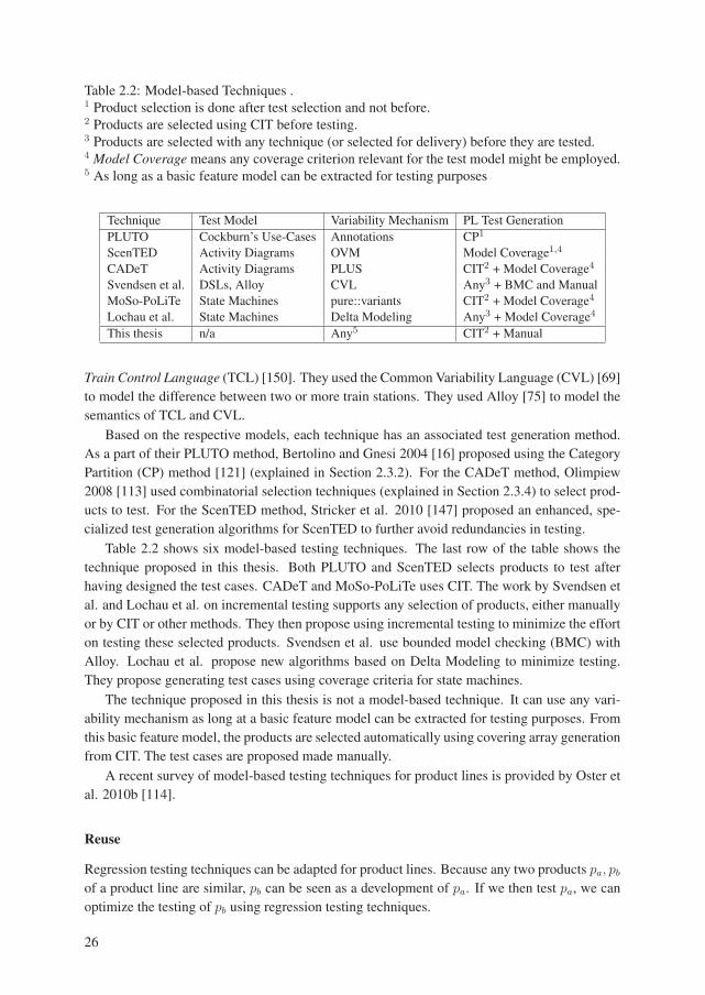
Table 2.2: Model-based Techniques .1 Product selection is done after test selection and not before.2 Products are selected using CIT before testing.3 Products are selected with any technique (or selected for delivery) before they are tested.4 Model Coverage means any coverage criterion relevant for the test model might be employed.5 As long as a basic feature model can be extracted for testing purposes

Technique Test Model Variability Mechanism PL Test Generation

PLUTO Cockburn’s Use-Cases Annotations CP1

ScenTED Activity Diagrams OVM Model Coverage1,4

CADeT Activity Diagrams PLUS CIT2 + Model Coverage4

Svendsen et al. DSLs, Alloy CVL Any3 + BMC and Manual

MoSo-PoLiTe State Machines pure::variants CIT2 + Model Coverage4

Lochau et al. State Machines Delta Modeling Any3 + Model Coverage4

This thesis n/a Any5 CIT2 + Manual

Train Control Language (TCL) [150]. They used the Common Variability Language (CVL) [69]

to model the difference between two or more train stations. They used Alloy [75] to model the

semantics of TCL and CVL.

Based on the respective models, each technique has an associated test generation method.

As a part of their PLUTO method, Bertolino and Gnesi 2004 [16] proposed using the Category

Partition (CP) method [121] (explained in Section 2.3.2). For the CADeT method, Olimpiew

2008 [113] used combinatorial selection techniques (explained in Section 2.3.4) to select prod-

ucts to test. For the ScenTED method, Stricker et al. 2010 [147] proposed an enhanced, spe-

cialized test generation algorithms for ScenTED to further avoid redundancies in testing.

Table 2.2 shows six model-based testing techniques. The last row of the table shows the

technique proposed in this thesis. Both PLUTO and ScenTED selects products to test after

having designed the test cases. CADeT and MoSo-PoLiTe uses CIT. The work by Svendsen et

al. and Lochau et al. on incremental testing supports any selection of products, either manually

or by CIT or other methods. They then propose using incremental testing to minimize the effort

on testing these selected products. Svendsen et al. use bounded model checking (BMC) with

Alloy. Lochau et al. propose new algorithms based on Delta Modeling to minimize testing.

They propose generating test cases using coverage criteria for state machines.

The technique proposed in this thesis is not a model-based technique. It can use any vari-

ability mechanism as long at a basic feature model can be extracted for testing purposes. From

this basic feature model, the products are selected automatically using covering array generation

from CIT. The test cases are proposed made manually.

A recent survey of model-based testing techniques for product lines is provided by Oster et

al. 2010b [114].

Reuse

Regression testing techniques can be adapted for product lines. Because any two products pa, pbof a product line are similar, pb can be seen as a development of pa. If we then test pa, we can

optimize the testing of pb using regression testing techniques.

26

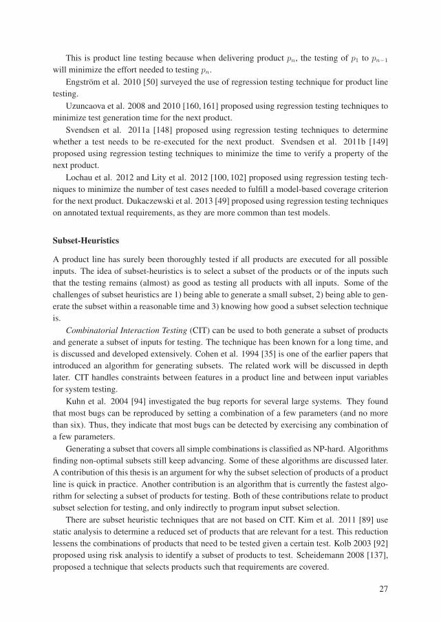
This is product line testing because when delivering product pn, the testing of p1 to pn−1

will minimize the effort needed to testing pn.

Engström et al. 2010 [50] surveyed the use of regression testing technique for product line

testing.

Uzuncaova et al. 2008 and 2010 [160, 161] proposed using regression testing techniques to

minimize test generation time for the next product.

Svendsen et al. 2011a [148] proposed using regression testing techniques to determine

whether a test needs to be re-executed for the next product. Svendsen et al. 2011b [149]

proposed using regression testing techniques to minimize the time to verify a property of the

next product.

Lochau et al. 2012 and Lity et al. 2012 [100, 102] proposed using regression testing tech-

niques to minimize the number of test cases needed to fulfill a model-based coverage criterion

for the next product. Dukaczewski et al. 2013 [49] proposed using regression testing techniques

on annotated textual requirements, as they are more common than test models.

Subset-Heuristics

A product line has surely been thoroughly tested if all products are executed for all possible

inputs. The idea of subset-heuristics is to select a subset of the products or of the inputs such

that the testing remains (almost) as good as testing all products with all inputs. Some of the

challenges of subset heuristics are 1) being able to generate a small subset, 2) being able to gen-

erate the subset within a reasonable time and 3) knowing how good a subset selection technique

is.

Combinatorial Interaction Testing (CIT) can be used to both generate a subset of products

and generate a subset of inputs for testing. The technique has been known for a long time, and

is discussed and developed extensively. Cohen et al. 1994 [35] is one of the earlier papers that

introduced an algorithm for generating subsets. The related work will be discussed in depth

later. CIT handles constraints between features in a product line and between input variables

for system testing.

Kuhn et al. 2004 [94] investigated the bug reports for several large systems. They found

that most bugs can be reproduced by setting a combination of a few parameters (and no more

than six). Thus, they indicate that most bugs can be detected by exercising any combination of

a few parameters.

Generating a subset that covers all simple combinations is classified as NP-hard. Algorithms

finding non-optimal subsets still keep advancing. Some of these algorithms are discussed later.

A contribution of this thesis is an argument for why the subset selection of products of a product

line is quick in practice. Another contribution is an algorithm that is currently the fastest algo-

rithm for selecting a subset of products for testing. Both of these contributions relate to product

subset selection for testing, and only indirectly to program input subset selection.

There are subset heuristic techniques that are not based on CIT. Kim et al. 2011 [89] use

static analysis to determine a reduced set of products that are relevant for a test. This reduction

lessens the combinations of products that need to be tested given a certain test. Kolb 2003 [92]

proposed using risk analysis to identify a subset of products to test. Scheidemann 2008 [137],

proposed a technique that selects products such that requirements are covered.

27

Oster et al. 2009 [118] proposed a method where feature models (FMs) and classification

trees (CT) are combined to a Feature Model for Testing (FMT). Classification trees are used in

the CT-method [62] for software testing. The FMT model can be used with classification tree

tools such as CTE [3] to generate a subset of system tests that also exercise the product line.

2.3.2 Product Line Use case Test Optimization (PLUTO)

The Product Line Use case Test Optimization PLUTO is “a test methodology for product fami-

lies” [14]. The PLUTO method was first introduced by Bertolino and Gnesi 2003 [15] and later

in Bertolino and Gnesi 2004 [16] and Bertolino et al. 2006 [14].

PLUTO, a model-based technique, uses Cockburn’s use cases [34] extended with variabil-

ity information. These enhanced use cases are called Product Line Use Cases, or PLUCs.

Cockburn’s use cases are represented in a textual notation with natural language. Variability

information is added as textual annotations.

A modified version of the category partition method (CP) is applied to the product line use

cases (PLUCs) in order to design a product line test suite. Before explaining how this is done,

product line use cases are explained.

Product Line Use Cases (PLUCs)

Figure 2.13 shows a product line use case (PLUC). There are two main sections: before and

after "PL Variability Features", both written in natural language. Above is a use case. This use

case has been annotated with variability information that is defined below. This particular use

case is for the call answer feature of a mobile phone, written on the first line. The goal in this

use case is to answer an incoming call on a mobile phone. The goal is annotated with "[CA0]".

Below, we can see that there are three alternatives for this annotation, Model 1–3.

When this and the other annotations are specified, we get a Product Use Cases (PUCs) [14].

This must be done manually. The "[CA0]" annotation can be directly replaced by one of the

model names, making for example "Goal: answer an incoming call on aModel 1 mobile phone".

Step 2 of the main success scenario is less simple. If the selected phone model is Model 1,

then a value for "[CA2]" must also be specified. If, say, "a" is chosen, then "[CA1]" becomes

"Procedure B". Thus, Step 2 of the main success scenario becomes "2. The system establishes

the connection by following Procedure B."

The PLUC in Figure 2.13 yields 5 different PUCs: for (CA0, CA1, CA2), we can have

(0, A, a), (1, B, a), (1, C, b), (2, B, a) and (2, C, b). Not all of these necessarily need to be

instantiated for testing. This depends on the application of category partition to PLUCs.

Using CP on PLUCs

PLUTO involves using CP on PLUCs to produce a product line test suite. CP is first applied

normally to the use case. Then, after having selected categories and choices, the products

corresponding to the choices made are selected. It might be the case that each test gets its

unique product, or it might be the case that all tests are run on a single product. This depends

on what is in the use case. One consequence of this is that no more products are needed than

there are test cases. In PLUTO, product selection is a consequence of applying the CP method.

28

PLUC CallAnswerGoal: answer an incoming call on a [CA0] mobile phoneScope: the [CA0] mobile phonePrecondition:

Signal is available.Mobile phone is switched on.

Trigger: incoming callPrimary actor: the userSecondary actors: the {[CA0] mobile phone} (the system)

the mobile phone company

Main success scenario:1. The user accepts the call by pressing the button "Accept".2. The system establishes the connection by following the {[CA1]

appropriate} procedure.

Extensions:1a. The call is not accepted:

1a.1. The user presses the button "Reject".1a.2. Scenario terminates.

PL Variability Features:CA0: Alternative:

0. Model 01. Model 1 [CA2]2. Model 2 [CA2]

CA1: Parametric:case CA0 of:

0: Procedure A:2.1 Connect caller and callee.

1 or 2:if CA2 = a then Procedure B:

2.1 Interrupt the game.2.2 Connect caller and callee.

if CA2 = b then Procedure C:2.1 Save current game status.2.2 Interrupt the current game.2.3 Connect caller and callee.

CA2: Alternative:a. Games are available; if interrupted, status is not saved.b. Games are available; if interrupted, status is saved.

Figure 2.13: Example of Product Line Use Case (PLUC) (taken from [14] and fixed)

29

For example, ten test cases of the use case in Figure 2.13 might only need three different

products out of the five possibilities: e.g. (0, A, a), (1, B, a), and (2, C, b). This is likely, because

all the options of all three alternatives are present in one of the three. If an eleventh test case

runs through 1 and b (for the second and third option respectively) then, of course, a product

with those is needed also, making it four.

2.3.3 Scenario-based Test Case Derivation (ScenTED)

Scenario based TEst case Derivation (ScenTED) was first introduced in Kamsties et al. 2003b

[84]. It is “a solution for applying product line concepts to the testing process by providing

detailed guidelines on how to create generic test artifacts in domain engineering and how to

reuse these generic artifacts in application engineering” [131].

The idea of ScenTED is to create test assets in UML which can be reused after deriving

products, also modeled in UML with variability specified using an orthogonal variability model

(OVM). In order to achieve this, they start by creating UML use case scenarios—descriptions

of how to use the software—that includes variation points (Figure 2.14, Step A). These are

UML activity diagrams with variability information as annotated branches. From these they ex-

tract test-case scenarios—a selection of paths through the activity diagrams just described (Fig-

ure 2.14, Step B). These are modeled as UML interaction diagrams with variability information

as annotated messages. They suggest a branch coverage criterion, modified for variability, to

select good test cases from the activity diagram. These test-case scenarios get their variability

resolved to become tests for products (Figure 2.14, Step C).

Figure 2.15 shows the information model of ScenTED. Here we find the use case and test-

case scenarios described above. In addition there are the architecture scenarios and executable

test cases. The former are scenarios with interactions between components—and not just the

user and the system as is the case for use case scenarios. The latter are the test-case scenarios

including concrete data for the input and output values of the tests.

The arrows between the boxes in Figure 2.15 are traceability links. Traceability in this

context means that you can find your way to, for example, the use case from a particular use

case scenario. The system is, as can be seen from the figure, traceable all around.

A thorough presentation of ScenTED can be found in [131] which is also the primary ref-

Figure 2.14: Main Activities and Artifacts of ScenTED – taken from [107]

30

Use Case

Use CaseScenario

ArchitectureConfiguration

ArchitectureScenario

Test CaseDesign

Test CaseScenario

Requirements Architecture Test

RuntimeSystem

ExecutableTest Case

ExecutableArtifacts Artifacts Artifacts Artifacts

Figure 2.15: ScenTED Information Model – taken from [131]

erence of this presentation of ScenTED. The ScenTED method was, prior to the primary refer-

ence, presented in [107], [129], [85] and [84]. The activity diagrams extended with variability

were presented earlier in [130].

Pohl and Metzger 2006 [126] is a short paper that discusses three challenges with SPL

testing and presents six principles which can be used to solve these challenges. The solutions

presented are compared against the ScenTED method where most of the principles are reported

to be addressed by ScenTED.

Reis et al. 2006 [128] presents an extension of ScenTED for performance testing called

ScenTED-PT. They explain how test assets for performance testing are derived and reused in

their extended method.

Stricker et al. 2010 [147] presents another extension of ScenTED called ScenTED-DF for

avoiding redundant testing.

2.3.4 Combinatorial Interaction Testing (CIT)

Combinatorial interaction testing [42] is an approach for performing interaction testing between

the features in a product line. The approach deals directly with a basic feature model to derive

a small subset of products which can then be tested using single-system testing techniques, of

which there are many good ones (see for example [18] or [83].)

The idea is to select a small set of products where the interaction faults are most likely to

occur. An important motivation for CIT is a paper by Kuhn et al. 2004 [94]. They investigated a

number of highly configurable industrial systems, and found that most of the bugs reported can

be attributed to a specific assignment of a few parameters. This means that by adjusting just a

few parameters, most bugs can be found. These empirical investigations apply to configuration

options also.

Figure 2.16a shows a feature model. If there is a fault in GIT that can be detected in any

product that contains this one feature, the fault is called a 1-wise fault. In Figure 2.16b, however,

there is a fault in the interaction between GIT and Zip that can be detected in any product that

include these two features. This 2-wise fault is not a fault in either feature, but a fault in the

interaction between them. They do not interact correctly. Surely, if they never interact either

directly or indirectly, there can be no such fault, but in this case they can: The Zip feature

allows browsing a zip-file and editing its internals. The GIT feature is a source control system.

31

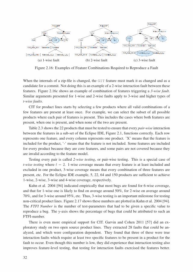
(a) 1-wise fault (b) 2-wise fault (c) 3-wise fault

Figure 2.16: Examples of Feature Combinations Required to Reproduce a Fault

When the internals of a zip-file is changed, the GIT feature must mark it as changed and as a

candidate for a commit. Not doing this is an example of a 2-wise interaction fault between these

features. Figure 2.16c shows an example of combination of features triggering a 3-wise fault.Similar arguments presented for 1-wise and 2-wise faults apply to 3-wise and higher types of

t-wise faults.CIT for product lines starts by selecting a few products where all valid combinations of a

few features are present at least once. For example, we can select the subset of all possible

products where each pair of features is present. This includes the cases where both features are

present, when one is present, and when none of the two are present.

Table 2.3 shows the 22 products that must be tested to ensure that every pair-wise interactionbetween the features in a sub-set of the Eclipse IDE, Figure 2.1, functions correctly. Each row

represents one feature, and every column represents one product. ’X’ means that the feature is

included for the product, ’-’ means that the feature is not included. Some features are included

for every product because they are core features, and some pairs are not covered because they

are invalid according to the feature model.

Testing every pair is called 2-wise testing, or pair-wise testing. This is a special case of

t-wise testing where t = 2. 1-wise coverage means that every feature is at least included and

excluded in one product, 3-wise coverage means that every combination of three features are

present, etc. For the Eclipse IDE example, 5, 22, 64 and 150 products are sufficient to achieve

1-wise, 2-wise, 3-wise and 4-wise coverage, respectively.

Kuhn et al. 2004 [94] indicated empirically that most bugs are found for 6-wise coverage,

and that for 1-wise one is likely to find on average around 50%, for 2-wise on average around

70%, and for 3-wise around 95%, etc. Thus, 3-wise testing is an important milestone for testing

non-critical product lines. Figure 2.17 shows these numbers are plotted in Kuhn et al. 2004 [94].

The FTFI Number is the number of test-parameters that had to be given a specific value to

reproduce a bug. The y-axis shows the percentage of bugs that could be attributed to such an

FTFI-number.

There is even more empirical support for CIT. Garvin and Cohen 2011 [57] did an ex-

ploratory study on two open source product lines. They extracted 28 faults that could be an-

alyzed, and which were configuration dependent. They found that three of these were true

interaction faults which require at least two specific features to be present in a product for the

fault to occur. Even though this number is low, they did experience that interaction testing also

improves feature-level testing, that testing for interaction faults exercised the features better.

32

Table 2.3: Pair-wise coverage of the feature model in Figure 2.1 the test suites numbered

Feature\Product 1 2 3 4 5 6 7 8 9 10111213141516171819202122

EclipseSPL XXXXXXXXXX X X X X X X X X X X X X

WindowingSystem XXXXXXXXXX X X X X X X X X X X X X

Win32 - - X - - X - - X - - - - - X - - - - - - X

GTK - X - - - - X - - X - - - X - - X - - - - -

Motif - - - - X - - X - - - X - - - - - - X - - -

Carbon - - - X - - - - - - X - - - - X - X - - - -

Cocoa X - - - - - - - - - - - X - - - - - - X X -

OS XXXXXXXXXX X X X X X X X X X X X X

OS_Win32 - - X - - X - - X - - - - - X - - - - - - X

Linux - X - - X - XX - X - X - X - - X - X - - -

MacOSX X - - X - - - - - - X - X - - X - X - X X -

Hardware XXXXXXXXXX X X X X X X X X X X X X

x86 X - - XX - - X - X X X - - X X - X X - - -

x86_64 - XX - - XX - X - - - X X - - X - - X X X

Team - - - - - XXXXX X X X X X X X X X X X X

CVS - - - - - - - - - - - - - - X X X X X X X X

CVS_Over_SSH - - - - - - - - - - - - - - - X X X X X X X

CVS_Over_SSH2 - - - - - - - - - - - - - - - - X X X X X X

SVN - - - - - XXXXX X X X X X X - X X X X X

Subversive - - - - - - - - - - X X X X X - - - - - - X

Subclipse - - - - - XXXXX - - - - - X - X X X X -

Subclipse_1_4_x - - - - - - - XXX - - - - - X - - - - X -

Subclipse_1_6_x - - - - - XX - - - - - - - - - - X X X - -

GIT - - - - - - - - - X - - - - - X X - X X - X

EclipseFileSystem XXXXXXXXXX X X X X X X X X X X X X

Local XXXXXXXXXX X X X X X X X X X X X X

Zip - - - XX - - - X - - - - X - - - - - X - X

These observations strengthen the case for combinatorial interaction testing.

Steffens et al. 2012 [146] did an experiment at Danfoss Power Electronics. They tested the

Danfoss Automation Drive which has a total of 432 possible configurations. They generated a 2-

wise covering array of 57 products and compared the testing of it to the testing all 432 products.

This is possible because of the relatively small size of the product line. They mutated each

feature with a number a mutations and ran test suites for all products and the 2-wise covering

array. They found that 97.48% of the mutated faults are found with 2-wise coverage.

There are three main stages in the application of combinatorial interaction testing to a prod-

uct line. First, the feature model of the system must be made. Second, the subset of products

must be generated from the feature model for some coverage strength. Such a subset is called

a t-wise covering array for a coverage strength t. Lastly, a single system testing technique must

be selected and applied to each product in this covering array.

Covering Arrays

The set of products that must be tested in combinatorial interaction testing is called a covering

array, but what precisely are covering arrays? A formal description should clarify.

An assignment a is a pair (f, included), where f is a feature of a feature model FM , and

included is a Boolean specifying whether f is included or not. A configuration, C, is a set

of assignments where all features in the feature model, FM , have been given an assignment.

33

Figure 2.17: Faults Attributed to Interactions - taken from [94]

A t-set is a set of t assignments, {a1, a2, ...}. The set of all t-sets of a feature model, FM , is

denoted Tt, e.g. T1, T2, T3, .... The set of invalid t-sets is denoted It, e.g. I1, I2, I3, .... The set

of valid t-sets is thus Ut = Tt \ It. A covering array of strength t is a set of configurations, Ct,

in which all valid t-sets, all t-sets in Ut, are a subset of (or the same set as) at least one of the

configurations.

The generation of covering arrays is a topic of many publications. Nie and Leung 2011 [109]

is a recent survey of combinatorial testing. They state that their survey is the first complete and

systematic survey on this topic. They found 50 papers on the generation of covering arrays.

A detailed comparison between three leading algorithms and the algorithm contributed in

this thesis (ICPL) is provided in Section 2.4.

2.3.5 Customizable Activity Diagrams, Decision Tables, and Test specifi-cations (CADeT)

The Customizable Activity Diagrams, Decision Tables, and Test Specifications (CADeT) method

was introduced by Olimpiew in [113] and is a "test design method that can be used to create

functional test specifications for SPLs".

There are four phases of CADeT: Phase I is to create activity diagrams from use cases.

The use cases have already been made as PLUS requirement models, introduced by Gomaa

et al 2005 [60]. Phase II is to create decision tables (as described by Binder 1999 [18]) and

test specifications from these activity diagrams. Phase III is to define and apply a feature-

based coverage criteria; CADeT proposes to use a combinatorial selection technique as used in

combinatorial interaction testing. Finally, Phase IV is to derive tests based on the decision table

and the test specifications.

34

2.3.6 Model-driven Software Product Line Testing (MoSo-PoLiTe)

Model-driven Software Product Line Testing (MoSo-PoLiTe) was introduced by Oster et al.

2009 [118] and further enhanced and developed later, including Oster et al. 2010 [117], Oster et

al. 2010b [114], Perrouin et al. 2011 [123], Oster et al. 2011 [119] and Oster et al. 2011b [120].

Oster 2012 [115] describes the state of the art of MoSo-PoLiTe as of 2012. An overview

of it can be seen in Figure 2.18. MoSo-PoLiTe is a model-based testing technique. It uses

combinatorial techniques to subset the products of a product line. These are then tested with

tests generated from a test-model. The method starts with a feature model and a test model.

The feature model is modeled using pure::variants (developed by pure::systems), and is seen

center-top in Figure 2.18. The test model is a union of behavior of all products, known as a

150% model. This behavior is modeled using Rational Rhapsody (developed by IBM) shown

in the top-right.

The variability modeled in the feature model is bound to the 150%model using pure::variants

Figure 2.18: MoSo-PoLiTe Overview – taken from [115]

35

integration with Rational Rhapsody. This is shown with the two-way arrow between the feature

model and the 150% model.

First, a subset of products for testing is generated. This is shown as the left side. First, the

pure::variants feature model is parsed into an Eclipse Plug-in tool. Then, the MoSo-PoLiTe

covering array generation algorithm is applied. This algorithm is covered and discussed in

Section 2.4.2. This results in a list of configurations, shown in the lower-left.

These configurations are then imported back into pure::variants as feature model configura-

tions. This is shown as a black arrow going from the configurations and up into the center. This

results in the variant models. They can now be used to instantiate product test models, or 100%

model. This is shown on the right side. There are bindings between these product models and

the configurations.

Then the tests need to be generated. They are generated using the Rational Rhapsody Auto-

matic Test Generation (ATG). These test suites can then be executed on the products built from

the configurations, shown in the lower-center.

2.3.7 Incremental Testing

Say an organization provides products of a product line. When a new product is requested, this

product is thoroughly tested from scratch. Because this new product, being a product of the

product line, is similar to the previously tested products, it should be possible to significantly

reduce the effort of testing this new product. Incremental testing for product lines proposes to

reduce the effort significantly.

Incremental testing for product lines was first presented in Uzuncaova et al. 2008 [161]

based on Alloy [75] and AHEAD [9]. Later, Svendsen et al. 2011a [148] proposed basing

incremental testing on CVL [69], and Lochau et al. 2012 and Lity et al. 2012 [100, 102]

proposed basing incremental testing on delta modeling [33].

Figure 2.19, from the original paper by Uzuncaova et al. 2008 [161], depicts the basic idea

of incremental testing for product lines.

A company that organizes and offers products using a product line strategy wants to ensure

that all the utilized products are of high quality. The way this is proposed done with incremental

testing is as follows. s0 is the formal specification of a product p0. This product, which can be

any product of the product line, is referred to as the base product or the core product.

Even though any product can in principle be chosen as the base product, some have noted

possible benefits of strategically selecting it. For example, Svendsen et al. 2010 [152] sug-

τ́

s0 s3

t3t0

Δs

Δt

ττ

Figure 2.19: Incremental Testing as Described by [161]

36

gests selecting the base product such that the difference between it and any other product is

minimized.

A test case t0 can be generated using test generator τ from the specification s0 of the product

p0. Another product, say p3, has a different specification s3. From s3 the test generator τ

generates the test t3.

Now, we can see p3 as a development from p0. Thus, we have a relationship between product

line testing and regression testing [2]. Regression testing aims at minimizing the effort needed

to retest a product that has changed.

We can capture the change between the specification s0 and s3 asΔs and the change between

test t0 and t3 as Δt.

Uzuncaova et al. 2008 and 2010 [160,161] proposed an algorithm τ ′ that allows following a

different path. Instead of generating the test t3 from s3 using the test generator τ , they propose

generating Δt from Δs using the algorithm τ ′. Then, by applying Δt to t0 we get t3. They

notice that this path takes less computational time than generating the test t3 from s3 using τ .

Uzuncaova et al. 2008 and 2010 [160, 161] used Alloy [75] to model the specifications siand AHEAD [9] for modeling the differences between the specifications, Δs, and to produce

the new specification based on the difference.

Svendsen et al. 2011a [148] addressed a different aspect of incremental testing. Their case

study was a product line of train stations. Train stations have rails, of course, and a lighting

system automatically organized by a software system. ABB, being the company in charge of

developing this software, tests each train station thoroughly from scratch.

Svendsen et al. proposed using incremental testing to lessen the effort of testing a second,

third, etc. train station by inferring which test cases needed to be rerun given that a previous,

similar train station had already been thoroughly tested. They had a DSL called the Train

Control Language (TCL) [150] in which the train stations were modeled. Instead of using

AHEAD as Uzuncaova et al., Svendsen et al. used the Common Variability Language (CVL)

[69] to capture the difference between two or more train stations.

As Uzuncaova et al., Svendsen et al. also used Alloy to model the semantics; in their case,

the semantics of TCL and CVL. They showed for their case study (to a limited extent) which

functionality was affected by a change from one station to another. Thus, if the first train station

had been thoroughly tested, they could tell (to a limited extent) which tests did and did not

need to be re-executed. The change of functionality was termed the semantic ripple effects of achange of a product, in this case, a train station.

Svendsen et al. 2011b [149] addressed yet another different aspect of incremental testing.

If a property p of a train station ts1 has been established to always hold for ts1, based on the

change from ts1 to another product, say ts2, modeled in CVL, they showed (to a limited extent)

how to determine if that property also holds for the second product, ts2.

Lochau et al. 2012 and Lity et al. 2012 [100,102] introduced incremental testing of product

lines based on delta modeling [33]. They address a different aspect of incremental testing than

Uzuncaova et al. and Svendsen et al. did.

Say an organization maintains a product line. They have one base product p that they have

tested with a test suite ts containing test cases {tc1, tc2, ..., tcn}. The test suite is generated from

the test model tm of the product p based on a coverage criterion C. The coverage criterion C is

captured as a set of test goals tg.

37

Because the base product was tested with test suite ts, the test plan tp for the core product p

simply is ts. This might not be the case for a second, third, etc. product of the product line.

When a second product needs testing, say product p′, the difference between the test assets

of p and p′, called ta and ta′ respectively, is captured as a tuple of deltas as follows:

δta,ta′ = δtm,tm′ , δtg,tg′ , δts,ts′ , δtp,tp′

When constructing the test plan tp′ for the second product p′, the fact that the first product was

tested with tp can be taken into account to minimize tp′.Lochau et al. 2012 and Lity et al. 2012 [100, 102] proposed modeling the test model as a

state machine and the test cases as paths in this state machine. Thus, the test goals are elements

of the state machine and the test suite is the set of all test cases satisfying these goals.

The deltas are proposed created using delta modeling [33, 135]. The test assets are all

constructed out of elements of a state machine; thus, the deltas are additions and removals of

these elements.

Based on the test models and the deltas, they did a case study where test cases were not

transferred from tp to tp′ if they had automatically determined that the test case was obsolete or

if the test case tested something that had not been impacted by the change in the test model. Of

course, test cases that is relevant for p′ that were irrelevant for p is added to tp′.The case study compared the size of the test plans to an application of a combinatorial

testing technique. For the combinatorial testing technique, the relevant tests were run for each

product. The case study showed that the average number of test cases for combinatorial testing

was 64, while that number was reduced to 19 using their incremental technique, 10 being new

and 9 being reused.

Dukaczewski et al. 2013 [49] observed that, in industry, formal test models rarely exist;

thus, the incremental technique proposed by Lochau et al. and Lity et al. is not straight-forward

to apply in industry. Dukaczewski et al. propose to apply the techniques on the requirements

instead. First, the requirements and the test cases, written in natural language, are manually

modeled as formal constructs and related to each other. Then, delta modeling can be applied to

these formal models in order to reduce the testing efforts.

2.4 Related Work: Algorithms for Covering ArrayGeneration

Three state of the art algorithms for covering array generation are IPOG, CASA and MoSo-

PoLiTe. In this section, these three algorithms will be described in detail and compared with

each other and to the contribution of this thesis.

These three algorithms were chosen because they fulfill criteria that are needed to perform

the extensive, automated, reproducible comparison done in Contribution 2 of this thesis:

1. it must be freely available

2. it must allow programmatic invocation

3. it must at least support 2 and 3-wise covering array generation

4. it was the latest development of that algorithm

38

5. it must have some support for constraints

Other algorithms that fulfilled these criteria but that were not included in our detailed compari-

son were ATGT [23], Microsoft PICT [46] and Grieskamp’s algorithm [61].

Comparisons between these algorithms and CASA exist in the literature. Thus, it is possible

to do an implicit, indirect comparison. ATGT is compared to PICT and an earlier version of

CASA in [26]. A comparison of Grieskamp’s algorithm with PICT and an earlier version of

CASA are included in [61].

2.4.1 IPOG

In Contribution 2 of this thesis, the tool NIST ACTS version 2 beta, revision 1.5 (acquired

2012-01-04) was compared to SPLCATool v0.3 (SPLC 2012) with respect to covering array

generation.

The version of NIST ACTS we had was closed source, so it is unknown exactly how the

algorithm is implemented in the tool. We ran the tool by selecting the option named "ipog",

which, according to the documentation of the tool [5], was the only option with support for

constraints. It implements some version of the IPOG algorithm. The In Parametric OrderGeneral (IPOG) algorithm [96, 97] is a development of the In Parametric Order (IPO) [98]

algorithm. In addition to selecting "ipog", we set the optimization level to 5 and the fast modeto "on".

Note that there are several algorithms implemented in NIST ACTS and discussed in e.g.

[97]. The tool in particular implements "ipog", "ipog_d", "bush", "paintball", "ipof" and "ipof2"

[5]. Again, only the option "ipog" supports constraints.

Both Lei et al. 2008 [97] and Lei et al. 2007 [96] describe a version of the IPOG algorithm

that do not handle constraints. Yu et al. 2013 [168] introduces the algorithm IPOG-C, which

introduces constraint handling into the IPOG algorithm in Lei et al. 2007 [96]. This paper was

published in March 2013 and cites Paper 2 of this thesis.

Thus, the latest paper on the IPOG algorithm was published by Lei et al. 2008 [97]. The

algorithm described in that paper in Section 3 will be discussed here. It is, however, not what

is implemented in NIST ACTS version 2 beta, revision 1.5 under the option "ipog", because it

actually handles constraints.

The Algorithm

Algorithm 1 shows the IPOG algorithm that is described in Lei et al. 2008 [97]. The algorithm is

explained in the same level of details in Lei et al. 2008 [97]. It does not support constraints, but

is the latest published algorithm before the acquisition of NIST ACTS version 2 beta, revision

1.5, which was used in our comparison.

It takes two parameters, an integer t and a set of parameters ps. The set of parameters is

assumed sorted with the parameters with the largest domain first. ps contain k parameters. Each

parameter is known as Pi for 1 ≤ i ≤ k.

The algorithm starts by adding every combination of the first t parameters to ts. Because

each combination is different, they must have one test set for each of them. The algorithm then

39

Algorithm 1 Generate a Covering Array with IPOG (no support for constraints):

IPOG(t, ps) : ts

1: ts ← a test for each combination of values of the first t parameters

2: for i = t+ 1; i ≤ k; i++ do3: π ← the set of all t-way combinations of values involving parameter Pi and any group of (t−1) parameters

among the first i− 1 parameters

4: for each τ = (v1, v2, ..., vi−1) in ts do5: choose a value vi of Pi and replace τ with τ ′ = (v1, v2, ..., vi−1, vi) so that τ ′ covers the most number

of combinations of values in π.6: remove from π the combinations of values covered by τ ′

7: end for8: for each combination σ in π do9: if there exists a test τ in test set ts such that it can be changed to cover σ then10: change τ to cover σ11: else12: add a new test to cover σ13: end if14: end for15: end for

proceeds to extend the test set one parameter at a time at Line 2, hence the name "In Parametric

Order".

Within the outer loop from Line 2–15, there are two inner loops. The first inner loop is the

extension to a new parameter, which is called horizontal growth. The second inner loop is the

extension of new test cases, which is called vertical growth.

Before these two loops are run, a set π is initialized to all combinations of t values of the

preceding i− 1 parameters including the values of the current working-parameter Pi.

The horizontal growth loop (Line 4–7) iterates through all test sets. Each test set get a value

of the current working parameter Pi such that it covers the most number of combinations in π.

On the next line, these newly covered combinations are removed from π.

The vertical growth loop (Line 8–14) iterates through all combinations σ in π. This loop

checks if a test can be changed to include the combination, Line 9, and, if it can, that test is

modified accordingly. It is possible to change a test without covering fewer combinations. The

reason is the presence of wild-cards. Changing a test means specifying the wild-card in order

to cover σ. If it cannot be changed, then a new test is added that covers σ, Line 12.

Comparison

These are the main similarities and differences between ICPL and IPOG as presented in Lei et

al. 2008 [97] and Algorithm 1.

• ICPL handles constraints, and IPOG does not.

• Both ICPL and IPOG approach the SCP problem (Set Cover Problem), of which covering

array generation is an instance, with a greedy polynomial time approximation algorithm

similar to that described by Chvátal 1979 [31].

• ICPL fills up an entire test greedily with as many uncovered combinations as possible

before it moves on to the next test. It then continues until all combinations are covered.

IPOG, in contrast, starts with i = t parameters and then covers all combinations of t

40

parameters of the first i parameters before it moves on to the (i+ 1)th parameter. It adds

tests when a combination does not fit any test. In other words, ICPL grows only vertically.

• Both IPOG and ICPL support parameters with multiple values. They support them, how-

ever, in different ways. ICPL supports them by a constraint saying that only one of a

set of values can be set to true. i.e. ICPL supports multiple values through the alter-

native construct: v1, . . . , vk are the k values of P , and they are constrained as follows:

((v1∨· · ·∨vk) ⇔ P )∧∧i<j ¬(vi∧vj). IPOG supports multiple values by having unique

assignments to a parameter from a domain. The alternative construct used in ICPL might

look more complicated than just having a parameter with a wide domain, but the construct

is dealt with easily by SAT solvers: Either one value is set to true, and the whole construct

passes, or else it does not.

• ICPL stores uncovered combinations in a Java HashSet. This set shrinks as more and

more t-sets are covered, making the algorithm run quicker as more t-sets are covered.

IPOG, on the other hand, stores the combinations in a special structure: Each parameter

combination has its own pointer in an array. This pointer points to a bit-map structure

that tells whether each value combination of the parameters is covered.

2.4.2 MoSo-PoLiTe

In Contribution 2 of this thesis, the tool MoSo-PoLiTe v1.0.5 plug-in (acquired 2012-01-25)

to pure::variants 3.0.21.369 (acquired 2012-01-02) was compared to SPLCATool v0.3 (SPLC2012) with respect to covering array generation.

The MoSo-PoLiTe plug-in was not openly available but was provided to us under a research

license. The source code was provided but under a non-disclosure agreement.

In Perrouin et al. 2011 [123], it was reported that MoSo-PoLiTe generated a 3-wise covering

array from the feature model with 287 features. That covering array was of size 841. In our

experiments, we observed significantly longer execution times for MoSo-PoLiTe than what was

reported in Perrouin et al. 2011 [123], but it produced similar covering array sizes.

In personal correspondence with the authors, we determined that the version of MoSo-

PoLiTe used in Perrouin et al. 2011 [123] is most likely different from the version provided

to us. The version used Perrouin et al. 2011 [123] was not provided to us.

The version of MoSo-PoLiTe provided to us does not have a full support for constraints. It

does support require and exclude constraints, but it has no support for converting constraints

that can be rewritten as a conjunction of require and exclude constraints.

Within the provided system, several algorithms were implemented. We used the algorithm

implemented in the classes Pairwise_NoRP and Threewise after recommendation by the

creators. Pairwise_NoRP uses Hash sets and is not deterministic.

The Algorithm

Because the provided source of MoSo-PoLiTe is under a non-disclosure agreement, we have

chosen to describe the algorithm as published in the latest paper prior to us acquiring the imple-

mentation, Oster et al. 2010 [117]. The paper does not give any pseudo-code of the algorithm.

The algorithm is only briefly described in text. Thus, its details are unavailable.

41

The MoSo-PoLiTe algorithm consists of two parts: 1) flattening and 2) sub-set extraction.

The input of the algorithm is a basic feature model as describe in Table 2.1 except the proposi-

tional formula must be a conjunction of require and exclude constraints and not a general propo-

sitional formula. i.e. if a require b and c excludes d, then the constraint P is (a → b)∧(c → ¬d).The algorithm as described in the document only supports 2-wise covering arrays, thus a value

of t is not given.

The output of the algorithm is a set of configurations, i.e. a set of set of tuple(f, b) where f

is a feature name and b is a Boolean specifying whether the f is included or not.

Sub-Step 1: Flattening The first sub-step of MoSo-PoLiTe is to flatten the input to an inter-

mediate type of model that is then used as input to the second sub-step, the subset extraction.

The intermediate model is as follows. It is a tuple (P,C) where P is a set of parameters and

C is a constraint. Each parameter is a tuple (names, values) where names is a set of names

that comprise the parameter, and values is the set of values of the parameter. Only one value

can legally be assigned to a parameter. e.g. for Boolean parameters p, the two values are ¬pand p. e.g. if a parameter is mandatory, only one value is possible.

The constraint C is a conjunction of require and exclude constraints. The primitives of this

constraint are the values of the parameters.

In order to construct the intermediate model (P,C), a set of rules are applied to the tree

bottom-up. It is called ’flattening’ because for each application of a rule, the tree becomes

flatter. Eventually, the tree becomes entirely flat, at which point it fits into the intermediate

model.

Oster et al. 2010 [117] refers to an associated website [116] for the 16 rules that comprise

the flattening algorithm. These 16 rules include all possible situations that can occur in a valid

model for MoSo-PoLiTe. Thus, an application of these rules bottom-up guarantees a flat model

eventually.

For each rule, there is a grandparent node, one or two parent nodes and one or two child

nodes.

The first four rules deal with situations involving one mandatory child node. In all four

situations, the parent node is merged with the child node. The parent node thus becomes a set

of two or more node names.

The next tree rules deal with the situations involving one single optional child node. In

all three situations, the child node is added as a child to the grandparent node, and a require

constraint is added saying that the child requires the old parent node.

The final nine rules deal with the remaining situations utilizing similar substitutions.

Sub-Step 2: Subset Extraction The second sub-step is only briefly sketched. Oster et al.

2010 [117] states that this sub-step is done in a similar manner as IPO. IPO is similar to what

was described above as a part of the IPOG algorithm.

MoSo-PoLiTe reduces the set of combinations by looking at the constraint and the legal

parameter assignments. Its implementation of IPOG thus reduces the set of combinations that

are considered in the sub-steps of IPOG to those that are valid.

In addition, MoSo-PoLiTe applies a technique called ’forward checking’. They reference

Haralick and Elliott 1980 [65] for what this technique consists of. Forward checking means that

42

when a pair is considered added to a configuration, it is first confirmed that it will not inevitably

lead to an invalid configuration. The reason forward checking is required is that two pairs that

are valid might lead to an invalid configuration when added to the same configuration. Thus,

when covering a legal pair, it must be checked that it does not cause the configuration to become

invalid as a total.

Comparison

MoSo-PoLiTe as described in Oster et al. 2010 [117] has the following similarities and differ-

ences with IPOG as described in Lei et al. 2007 [96] and with ICPL.

• ICPL handles all propositional constraints; MoSo-PoLiTe supports binary constraints;

IPOG does not support constraints.

• ICPL handles propositional constraints using a SAT solver; MoSo-PoLiTe support con-

straints by excluding invalid pairs based on the binary constraints and using forward

checking.

• ICPL generates a propositional constraint from the basic feature model given to it; MoSo-

PoLiTe flattens its input into its own intermediate format.

• MoSo-PoLiTe can only generate 2-wise covering arrays. IPOG and ICPL can generate

t-wise covering arrays

• MoSo-PoLiTe approaches the SCP problem as both ICPL and IPOG, with a greedy poly-

nomial time approximation algorithm similar to that described by Chvátal 1979 [31].

• MoSo-PoLiTe covers one parameter at a time, similarly to IPOG; ICPL generates one

entire configuration at a time.

• For its intermediate format, MoSo-PoLiTe supports parameters with multiple values using

the alternative construct in the same way as ICPL. For the covering array generation,

however, the alternative construct is treated as a set of possible value assignments instead,

just as IPOG.

2.4.3 CASA

In Contribution 2 of this thesis, the tool Covering Arrays by Simulated Annealing (CASA) v1.1was compared to SPLCATool v0.3 (SPLC 2012) with respect to covering array generation.

This tool is free and open-source2, and it implements an algorithms described in Garvin et al.

2011 [59], a development of earlier results presented in Garvin et al. 2009 [58].

Before the work by Garvin et al., Simulated Annealing (SA) had been studied for some

time for the generation of covering arrays. The more general class of algorithms containing

simulated annealing is the meta-heuristic algorithms.

Nurmela and Östergård 1993 [110] used simulated annealing to construct covering designs,

which are similar to covering arrays. Stardom 2001 [145] investigated several meta-heuristic

algorithms for covering array generation including, simulated annealing, Tabu Search (TS) and

Genetic Algorithms (GA). Cohen et al. 2003 [43] and Cohen et al. 2003b [39] integrated the

previous work on simulated annealing with an algebraic approach for better covering array gen-

eration. Most of the early work on simulated annealing did not consider constraints. Cohen et

2http://cse.unl.edu/~citportal/tools/casa/, accessed 2013-05-29

43

al. 2007 [41] extended simulated annealing with a SAT solver in order to deal with constraints.

This forms the basis of which Garvin et al. 2009 [58] developed the algorithms for the CASA

tool.

The Algorithm

Garvin et al. 2011 [59] shows the pseudo code of a basic version of the simulated annealing al-

gorithm for covering array generation. They then proceeded to describe two main improvements

and six refinements to improve this algorithm. Except one, these improvements are described

textually. The improvements are, however, specific to the simulated annealing approach. Thus,

because the purpose here is to compare CASA with ICPL, MoSo-PoLiTe and IPOG, the basic

version of CASA will be described and compared with these three other algorithms.

Algorithm 2 shows the highest level of the basic CASA algorithm. It takes a value t for the

strength of the covering array. k is the number of parameters, and v is the number of values

for each parameter. C is the complete propositional constraint. lower and upper are the size

bounds within which a covering array will be searched for. For example, if lower is 1 and upper

is 10, a covering of size 5 might be found, being between 1 and 10.

Algorithm 2 Generate a Covering Array with CASA:

CASA(t, k, v, C, lower, upper) : A

1: A ← ∅2: N ← (lower + 2upper)/3�3: while upper ≥ lower do4: A′ ← anneal(t, k, v, C,N)5: if countNoncoverage(A′) = 0 then6: A ← A′

7: upper ← N − 18: else9: lower ← N + 110: end if11: end while

Algorithm 2 implements a binary search within the bounds. First, it makes a suggestion,

Line 2. For example, if lower is 1 and upper is 10, N is first set to (1+ 2·10)/3 = 7. Then, the

loop at Line 3-11 is run until the space has been delimited. It is delimited in two ways: Line 4

finds a valid array of configurations using the anneal method described later. If it is a complete

covering array, i.e. if there is no non-coverage, that solution is stored and the upper bound is

lowered. If, however, the coverage is incomplete, the lower bound is raised.

Algorithm 2 calls Algorithm 3. Algorithm 3 takes the values t, k, v and C directly from

Algorithm 2. N is the current intermediate between lower and upper. It returns an array of

products that may or may not be a covering array.

Algorithm 3 calls various methods that are given as pseudo-code: initialState, stabilized,

countNoncoverage, SAT and cool. The method starts by calling one of these functions,

initialState, in order to get an array of size N . Then, temperature is initialized to some

initial value. The main loop starting at Line 3 is continued until the stabilized method has

determined that the number of coverage has stabilized. The loop starts by selecting a random

row and column, and then it copies the array and modifies one of its entries by selecting a new

44

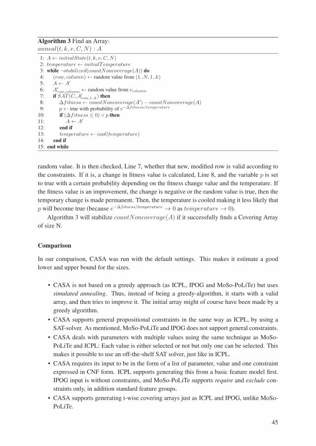
Algorithm 3 Find an Array:

anneal(t, k, v, C,N) : A

1: A ← initialState(t, k, v, C,N)2: temperature ← initialTemperature3: while ¬stabilized(countNoncoverage(A)) do4: (row, column) ← random value from (1..N, 1..k)5: A ← A′

6: A′row,column ← random value from vcolumn

7: if SAT (C,A′row,1..k) then

8: Δfitness ← countNoncoverage(A′)− countNoncoverage(A)9: p ← true with probability of e−Δfitness/temperature

10: if (Δfitness ≤ 0) ∨ p then11: A ← A′

12: end if13: temperature ← cool(temperature)14: end if15: end while

random value. It is then checked, Line 7, whether that new, modified row is valid according to

the constraints. If it is, a change in fitness value is calculated, Line 8, and the variable p is set

to true with a certain probability depending on the fitness change value and the temperature. If

the fitness value is an improvement, the change is negative or the random value is true, then the

temporary change is made permanent. Then, the temperature is cooled making it less likely that

p will become true (because e−Δfitness/temperature → 0 as temperature → 0).

Algorithm 3 will stabilize countNoncoverage(A) if it successfully finds a Covering Array

of size N.

Comparison

In our comparison, CASA was run with the default settings. This makes it estimate a good

lower and upper bound for the sizes.

• CASA is not based on a greedy approach (as ICPL, IPOG and MoSo-PoLiTe) but uses

simulated annealing. Thus, instead of being a greedy-algorithm, it starts with a valid

array, and then tries to improve it. The initial array might of course have been made by a

greedy algorithm.

• CASA supports general propositional constraints in the same way as ICPL, by using a

SAT-solver. As mentioned, MoSo-PoLiTe and IPOG does not support general constraints.

• CASA deals with parameters with multiple values using the same technique as MoSo-

PoLiTe and ICPL: Each value is either selected or not but only one can be selected. This

makes it possible to use an off-the-shelf SAT solver, just like in ICPL.

• CASA requires its input to be in the form of a list of parameter, value and one constraint

expressed in CNF form. ICPL supports generating this from a basic feature model first.

IPOG input is without constraints, and MoSo-PoLiTe supports require and exclude con-

straints only, in addition standard feature groups.

• CASA supports generating t-wise covering arrays just as ICPL and IPOG, unlike MoSo-

PoLiTe.

45

2.4.4 Other Algorithms

There are many papers on the problem of covering array generation. The website pairwise.

org lists 37 tools for covering array generation. Nie and Leung 2011 [109] had collected more

than 50 papers about the problem of covering array generation. Here are some of the other

algorithms for covering array generation.

According to our investigations, none of these algorithms perform better than ICPL when it

comes to generating t-wise covering arrays from large feature models with general propositional

constraints. This was recently seconded by Liebig et al. 2013 [99].

AETG The Automatic Efficient Test Case Generator (AETG) was an early algorithm for cov-

ering array generation presented in Cohen et al. 1994 [35], Cohen et al. 1996 [37] and Cohen

et al. 1997 [36]. It is currently available as a commercial product accessible via a subscription

based web interface3.

AETG is a greedy algorithm. It has some support for constraints by listing the illegal combi-

nations explicitly. It also has some support for generating the list of invalid combinations from

propositional formulas. Further details of the algorithm are, however, unavailable.

Cohen et al. 2006 [40] explained how combinatorial interaction testing though AETG could

be used to test product lines.

AllPairs The AllPairs tool [6] implements an algorithm for covering array generation. The

tool is freely available online4. It uses a greedy approach, and builds up the answer row by row.

ATGT The ASM Test Generation Tool (ATGT) was presented in Calvagna and Gargantini

2008 [23] and Calvagna and Gargantini 2009 [24]. The algorithm takes Abstract State Machines

(ASM) with constraints as input and produces a set of test cases for the ASMs. Constraints are

dealt with by invoking SAL, a bounded and symbolic model checker tool [47].

The tool is available online, freely5.

The Laboratory for Combinatorial Interaction Testing (CITLAB)6 was introduced by Cal-

vagna et al. 2012 [56], Calvagna et al. 2013a [28] and Calvagna et al. 2013b [27]. Just

as SPLCATool (the tool implementing the contributions of this thesis), it supports importing

feature models. However, instead of converting it to a propositional constraint, it converts it

to input to the multi-valued parameter formats used by AETG and IPOG. They used it as a

framework for comparing the performance of various algorithms for covering array generation

algorithms, including AETG, DDA, PairTest, CASA and IPOG.

DDA The Deterministic Density Algorithm (DDA) was introduced in Colbourn et al. 2004

[44] and in Bryce and Colbourn 2006 [21]. It is also a greedy algorithm with a new heuristic

3http://aetgweb.argreenhouse.com/, accessed 2013-05-284http://www.mcdowella.demon.co.uk/allPairs.html, accessed 2013-05-285http://cs.unibg.it/gargantini/software/atgt/atgt_smt_ccit.html, accessed 2013-

05-286Available at https://code.google.com/a/eclipselabs.org/p/citlab/, accessed 2013-05-

28

46

that makes it faster and more often accurate than four other algorithms they it was compared to

in an experiment: AETG, TCG, IPO and TConfig.

GTWay Zamli et al. 2011 [169] introduced an algorithm for covering array generation called

GTWay. Their algorithm supports concurrent execution, and performs better than the compared

algorithms for high coverage strength, t > 6. They compared GTWay with IPOG, Whitch,

Jenny, TConfig and TVG II. GTWay was a development of G2Way introduced in Klaib et al.

2008 [91]. It is a backtracking algorithm that tries to combine uncovered interactions in the best

possible way. It sets up the possible pairs in a similar structure as IPOG (discussed above).

IPOG-C Yu et al. 2013 [168] introduces the IPOG-C algorithm. It introduces constraint

handling into the IPOG algorithm in Lei et al. 2007 [96]. IPOG-C utilizes some optimization

techniques similar to those in ICPL in addition to some new techniques. (The paper cites Paper

2 of this thesis.)

mAETG mAETG was introduced in Cohen et al. 2003 [43]. It was extended with constrain

handling using a SAT solver in Cohen et al. 2007 [41] and Cohen et al. 2008 [42]. mAETG,

like AETG, is a greedy algorithm.

PACOGEN PACOGEN is an algorithm and a tool7 by Hervieu et al. 2011 [73]. It can gen-

erate covering arrays from constrained feature models. It uses constraint programming instead

of a SAT-solver to validate constraints. PACOGEN makes a constraint-solving problem out of

the problem of generating a 2-wise covering array from a specific feature model. It then runs a

branch-and-bound method to find a covering array.

Perrouin’s Algorithm Perrouin et al. 2010 [124] introduced an algorithm for covering array

generation that converted the problem of generating a covering array into a problem for Alloy

[75]. They presented several optimizations to make this quicker. In Perrouin et al. 2011 [123]

this algorithm was compared with MoSo-PoLiTe. They found that MoSo-PoLiTe was more

stable, was much faster and produced smaller covering arrays.

PICT Microsoft’s tool PICT implements an AETG-like algorithm that is optimized for speed.

It was introduced in Czerwonka 2006 [46].

Other There are even more algorithms: Calvagna’s Algorithm [29], Jenny [76], AETGm [38],

a Generic Algorithm (GA) and an Ant Colony Algorithm (ACA) was introduced in Shiba et

al. 2004 [143], PairTest [153], Grieskamp’s Algorithm [61], IPO-s [25], IBM Intelligent TestCase Generator (Whitch) CTS and TOFU [66], TConfig [167], TestCover [142] and Test CaseGenerator (TGC) [158].

7PACOGEN is available at http://hervieu.info/pacogen/ and http://www.irisa.fr/lande/gotlieb/resources/Pacogen/, accessed 2013-05-28

47

Chapter 3

Contributions

3.1 Overview and Relation to the State of the Art

Figure 3.1 shows a test process for product lines and where in this process this thesis contributes

(marked 1–5.) Three assets are needed before the test process can be applied: A feature diagram

(Asset A), an implementation (Asset B) and test cases (Asset C).

None of the contributions address the generation of tests (Asset C), in contrast to PLUTO,

ScenTED, CADeT, MoSo-PoLiTe and incremental testing. They address this issue in various

ways and also integrate this selection with product selection.

Contribution 1, 2 and 4 address the sub-setting of products for product line testing. Products

are proposed selected by combinatorial selection techniques as in CIT, MoSo-PoLiTe, CADeT

and some of the incremental testing approaches. Contribution 1 and 2 investigate and improve

the efficiency of algorithms for test product selection. The ICPL algorithm, described in Con-

tribution 2, enables the (2-wise) sub-setting of products for product lines with as much as 7,000

features, one of the largest documented product lines. Contribution 4 enables market-focused

selection and prioritization for product selection with combinatorial techniques.

Contribution 3 is a technique for using information in the implementation (Asset B) to im-

prove the testing of the selected products: Products that differ only in the implementations of

the homogeneous abstraction layers can be tested using the same test suites and their results can

be compared to form a voting oracle.

Finally, Contribution 5 addresses the automation of the entire testing process shown in Fig-

ure 3.1. Assuming the existence of the Asset A, B and C, the proposed algorithms and their

implementations automatically generate Asset D, E and F. The automated test process is demon-

strated by a fully automated application to the part of the Eclipse IDE maintained by the Eclipse

Project. Such a large-scale, fully reproducible and fully documented application of a product

line testing technique is not found in the existing literature on product line testing.

The idea of Contribution 5 is not necessarily to represent a finalized and all-encompassing

testing process, but rather to serve as a base-line for comparison and advancement of scalable

product line testing techniques.

The five contributions are covered in four sections. The generation of covering arrays from

large feature models (Contribution 1 and 2) is covered in Section 3.2, and then three advance-

ments of CIT (Contributions 3–5) are presented in sections 3.3–3.5 respectively.

49

Figure 3.1: Contributions 1, 2, 3, 4 and 5 as Parts of a Whole Test Process

3.2 Generation of Covering Arrays from Large FeatureModels

3.2.1 Difficulty of Covering Array Generation

The generation of t-wise covering arrays is generally regarded to be an intractable problem

[109]. This is arrived at through complexity analysis, with which it is classified as NP-hard.

The argument is: In order to get a set of valid products, one valid product must be found. A

basic feature model is expressively equivalent to a Boolean formula; thus, finding a single valid

product is equivalent to the Boolean satisfiability problem (SAT). This problem is the classic

NP-hard problem. NP-hard means the problem is at least as hard as the hardest problem in

NP [55].

In complexity analysis, an algorithm’s complexity is usually arrived at by considering the

worst of the valid inputs (worst-case analysis). This is of course useful when any input can

occur. However, such analysis can be too pessimistic when the context of a problem limits

which inputs will ever be presented to an algorithm.

SPLE-SAT is Easy

Such is the case for feature models in the context of software product line engineering (SPLE).

This was the main theme of our paper titled "Properties of Realistic Feature Models make

Combinatorial Testing of Product Lines Feasible" published at MODELS 2011 [78], Paper 1.

It is not unique for the SPLE context. In a series of publications starting with [30] and ending

50

in [17], it was established that the satisfiability problem is easy for Boolean formulas originat-

ing from realistic VLSI circuits (Very-Large-Scale Integration circuits). This sub-problem was

termed ATPG-SAT (Automatic Test Pattern Generation-SAT). These quotes from [30] should

make their reasoning clear:

It has been observed that SAT formulae derived fromATPG problems are efficiently

solvable in practice. This seems counter-intuitive since SAT is known to be NP-

Complete. This work seeks to explain this paradox. We identify a certain property

of circuits which facilitates efficient solution of ATPG-SAT instances arising from

them. In addition, we provide both theoretical proofs and empirical evidence to

argue that a large fraction of practical VLSI circuits could be expected to have the

said property.

and

Note that we are not generating arbitrary SAT formulae during ATPG; there is some

structural quality inherent in ATPG problems which makes them easy to solve.

Following the same style as ATPG-SAT, the sub-problem of SAT originating from realistic

feature models can be called SPLE-SAT.The role of feature models in SPLE is for potential customers to be able to configure a

product according to their needs. Had this been difficult, the customers could not do this.

Indeed, in the worst case, not a single product from the product line could be delivered. This

is absurd. In SPLE, feature models are easily configurable in order to serve their purpose.

Figure 3.2 shows the situation in a Venn diagram: Even though both SPLE-SAT the hard SAT

problems are both sub-sets of SAT, they do not necessarily intersect. Given that this situation is

true, SAT solvers can be used to configure feature models without risking intractability.

Figure 3.2: Although there are hard SAT problems, SPLE-SAT need not overlap the region.

Paper 1 establishes that SPLE-SAT is easy in two parts: the argument just put forth and an

empirical investigation. 19 realistic feature models were investigated. It was found that even

for the largest feature models publicly available, the Linux Kernel feature model, satisfiability

is quick, taking 125 ms with SAT4J. Indeed, the Linux kernel is meant to be configured by hand

(assisted by a SAT solver), something that is regularly done by advanced Linux users.

Earlier than our work, Mendonca et al. 2009 [106] had noticed that satisfiability for SPLE-

SAT for some reason was quick in practice. They did not provide an explanation for this,

however.

51

Covering Array Generation is Feasible

Now, given that SPLE-SAT is easy, generation of covering arrays then, by complexity analy-

sis, reduces to the set-cover problem (SCP). SCP is not NP-hard; it is actually NP-complete

and has a polynomial time approximation algorithm with an established and acceptable upper

bound [31]. This algorithm is a greedy approximation of SCP. Approximation, in this context,

means that there will be more products than optimally possible, but it also means that the num-

ber of products in the worst-case still is limited by some upper bound. The greedy algorithm

is quite simple: Select the configuration that covers the most uncovered interactions until all

interactions are covered. This algorithm needs to be modified for covering array generation

from feature models because the configuration space generally is exponential with respect to

the number of features. This additional stage is a contribution of Paper 1: This is solved by

greedily packing uncovered interactions into a configuration. This voids Chvátal’s upper bound

guarantee; however, we did investigate the impact of this as follows:

A tool was implemented, and a corpus of 19 feature models was collected. The experiment

is documented in Paper 1. In it, all 19 feature models were given to the tool, and 1–4-wise

covering arrays were attempted generated. It could be understood from the sizes of the feature

models in the corpus when a covering array would take too long to generate.

As just mentioned, the algorithm was based on a greedy approximation for the set-cover

problem (SCP). This basic algorithm was shown to have an acceptable upper bound [31]; but,

for feature models, due to their huge configuration space, this upper bound cannot be achieved.

Still, it was shown that for the realistic feature models, the covering arrays did stay within

an acceptable size. Due to the central role of a satisfiability solver within the algorithms, we

suggested that the algorithm was a good basis for a scalable algorithm for t-wise covering array

generation.

The algorithm’s performance is not compared with the other available algorithms for t-wise

covering array generation. The performance of this algorithm is, however, on par with the other

state of the art algorithm, as would be later documented in Paper 2, which contributions are

discussed next.

3.2.2 Scalable t-wise Covering Array Generation

Having established the tractability of SPLE-SAT and having a basic algorithm for covering

array generation with potentials for improvement, the basis was set for the development of a

scalable algorithm for t-wise covering array generation.

Such an algorithm was the contribution of our paper titled "An Algorithm for Generating

t-wise Covering Arrays from Large Feature Models" published at SPLC 2012 [79], Paper 2.

The algorithm named ICPLwas developed and implemented by profiling the basic algorithm

and speeding up its bottlenecks by an analysis of the situation creating the bottleneck. This

resulted in a range of optimizations presented in Section 3 and 4 of Paper 2. (The interested

reader is advised to read those sections at this point.)

To establish its performance, an evaluation and comparison was set up. The results of this

evaluation and comparison are reported in Section 5 of Paper 2. The performance of the al-

gorithm was compared to the basic algorithm from Paper 1, called "Algorithm 1", and three

52

of the leading algorithms for covering array generation: IPOG [96], CASA [59] and MoSo-

PoLiTe [117]. Thus, these five algorithms were compared: ICPL, Algorithm 1, IPOG, CASA

and MoSo-PoLiTe. This comparison is presented as the space permits in Paper 2. The re-

maining details and the additional diagrams are added as Appendix C. A detailed description

of IPOG, CASA and MoSo-PoLiTe is found in Section 2.4 including a qualitative comparison

with ICPL.

The evaluation of ICPL shows that only it can generate the 2-wise covering array from the

largest feature model available, the Linux Kernel, within a time limit of 12 hours. This feature

model is gigantic with 6,888 features and 187,193 clauses in its complete CNF-constraint.

The speed of each algorithm was measured by giving each algorithm three whole days to

generate 100 covering arrays for each feature model and for each strength: 1, 2 and 3. All

algorithms managed to do this for the same 16, 14 and 12 feature models for 1, 2 and 3-wise

covering arrays, respectively. A statistical analysis of these runs showed that ICPL’s time is

O(f 0.76) with respect to the number of feature in the feature mode, f , while the second fastest,

MoSo-Polite’s, time is O(f 1.75). For 3-wise covering arrays, ICPL’s time is O(f 1.14) against

O(f 2.62) for the second fastest, MoSo-PoLiTe.

For a feature model with 1,000 features, ICPL is almost 1,000 times faster than the second

best for 2-wise covering array generation, and ICPL is almost 30,000 times faster than the

second best for 3-wise covering array generation.

3.2.3 Consolidations

For this section of contributions, some consolidations can be noted.

• The existence and performance of ICPL are further arguments in favor of the claim of

Paper 1 that the generation of t-wise covering arrays from realistic feature models is

feasible in practice.

• Henard et al. 2012 [72] acknowledges that the tool developed for our MODELS 2011-

paper (SPLCATool v0.2) was a state of the art tool for covering array analysis and gen-

eration. They used it as the main comparison to their own contributed algorithms and

implementations.

• Paper 2 suggested that there were more optimizations possible for t-wise covering array

generation. Haslinger et al. 2013 [68] suggest additional improvements to speed up the

algorithm.

• Kowal et al. 2013 [93] further improves ICPL by adding a filtering step before running

ICPL. This filter filters out feature combinations that are known not to interact. They

show that this both decreases the time it takes to run ICPL and decreases the number of

products generated by ICPL.

• Liebig et al. 2013 [99] propose a variability aware analysis technique for validating prod-

uct lines. They evaluate their proposed technique by comparing it with three sampling

techniques, one being pair-wise sampling. For pair-wise sampling they chose the ICPL

algorithm proposed in Paper 2 of this thesis as implemented in SPLCATool. They re-

port that not only is this the fastest algorithm they could find for pair-wise covering array

generation, it was also the only algorithms that was scalable enough to be used in their

experiments.

53

3.3 Optimized Testing in the Presence of Homogeneous Ab-straction Layers

Cabral et al. 2010 [22] writes that "Alternative features [...] present a more difficult challenge

for testability. We argue that these are the true deterrents to testability since only one feature

can be present in an SPL at a time."

One type of common software construct causes alternative features in the product line’s fea-

ture model: homogeneous abstraction layers. Customers usually have a wide range of different

deployed software that provides essentially the same functionality: operating systems—with

their file handling, networking, virtual memory, threading and synchronization—databases,

with their obvious functionality; windowing systems, interfaces, hardware architecture, etc.

These all come in different variants (e.g. Windows, Linux, MacOS, etc.; Oracle, Microsoft

SQL, MySQL, PostgreSQL, etc; Windows, GTK, Motif, Photon, etc; Intel x86, Intel x86-64,

PowerPC, ARM, etc.), but provide essentially the same functionality.

A technique used to make a system run in different environments is to make an abstraction

layer that is implemented concretely for each particular system but that provides a uniform

way of interacting with them to the product line code. Thus, in order to make a product of a

product line function in a specific environment, we need to set up the right implementation of

the abstraction layer. The selection of such an implementation must be modeled as an alternative

feature.

Thus, when a product line is designed to be able to run in differing environments, its feature

model will have many alternative features. This again, deters the testability of the product line

with CIT.

We found a way to turn this problem into a benefit. Whenever alternative features due

to homogeneous abstraction layers cause a deterioration of the performance of combinatorial

interaction testing, it can be turned around and used to help testing instead. This result was

presented in the article titled "Bow Tie Testing: A Testing Pattern for Product Lines" published

in "Pattern Languages of Programs", the proceedings of the 16th European Conference, 20121

[80], Paper 3.

3.3.1 Description of the Technique

Because implementations of homogeneous abstraction layers are supposed to provide the same

functionality to the product line assets, we know that whatever concrete implementation is cho-

sen, the product will behave essentially the same. Thus, if a test case is run on two products that

only differ in their implementations of their homogeneous abstraction layers, the test will result

in essentially the same execution trace. Thus, we can compare the executions; if they differ, we

know that something is wrong. It is of course not limited to two products. If there are three or

more, we can construct a voting oracle [18]; if we know one of the executions are correct, we

can use it as a gold standard oracle [18].

We did implement tool support for the detection of such groups of products. Annotate a

feature model to inform the tool which alternative feature groups are due to a homogeneous

1This paper was published at a conference on patterns. The patterns community have several special require-

ments in the presentation of a pattern. In this part of the thesis, the pattern-style of presentation will not be used.

54

abstraction layer. Then, the tool will note groups of products that only differ beneath this layer.

3.3.2 Application to Finale’s Systems

Finale’s systems are systems for reporting various things about a company’s finances to the

government. This is required by the government to ensure that all the taxes are collected as

required.

Finale’s systems run on all versions of Windows that is supported by Microsoft. When we

worked with this case study, three different versions were supported on the client-side: Windows

XP SP3, Windows Vista SP2 and Windows 7. All come in 32-bit and 64-bit variants. Finale’s

systems had to run correctly on all systems with a graphical interface zoom level of 100%,

125% and 150%. On the servicer-side, four versions of windows were supported: Windows

2000, Windows 2003, Windows 2008 and Windows 2008 SR2. The major abstraction layer

was, however, towards the accounting systems. They supported 18 types of accounting systems,

all interacted with through a homogeneous abstraction layer.

If we want to exercise all pairs of interactions, all products containing a version of client-

side Windows paired with a version of an accounting system, then we need at least 6∗18 = 108

products. Indeed, the pair-wise covering array contains 116 products. If we group together

those products that only differ below a homogeneous abstraction layer, we reduce the number

to 60.

The Finale case was not documented in detail in Paper 3 because of confidentiality concerns.

Instead, we used the more open Eclipse IDE case study.

3.3.3 Application to the Eclipse IDEs

The Eclipse IDEs are used as a case study throughout this thesis. One aspect of the Eclipse

IDEs is given focus only in this part. Although Eclipse is programmed mostly in Java, it is

not completely so. The reason is that the programmers found it to be too slow. Thus, they

replaced the implementations of abstraction layers in Java with their own implementations. For

version 3.7.0, they supported six operating systems: Windows, Linux, MacOS X, Solaris, AIX

and hpux. These operating systems provided various windowing systems and ran on various

hardware architectures. In total, they support 16 combinations of hardware, windowing systems

and operating systems.

This caused the pair-wise covering array of the sub-set of the Eclipse IDEs used in this part

to grow to 41 products. Out of these, only 20 groups of products need to be tested with a unique

test suite, the rest differ only beneath the homogeneous abstraction layers. Covering the system

with 1-wise testing gives 10 products, but only 5 test suites are required. For 3-wise testing,

with 119 configurations, only 45 test suites are required.

It should be noted that if the other constructs in the feature model are the main cause the

covering array’s large size, then no benefits can be derived from the technique described here,

but, then, the alternative features are not the cause of the deteriorations either.

For more details on this and on the Eclipse IDE case, see Appendix E.

55

3.4 Market-Focused Testing based on Weighted Sub-Productline Models

The idea behind combinatorial interaction testing is to exercise all simple interactions. In some

cases, however, this implies some wasted effort. The product line’s market can limit which

products will occur. Then, there is no need to exercise all simple interactions.

In order to focus on the market-relevant interactions, the market situation must be captured

or modeled somehow. Such a model is a contribution of our paper titled "Generating Better

Partial Covering Arrays by Modeling Weights on Sub-Product Lines" published at MODELS

2012 [82], Paper 4. Relevant algorithms based on this new type of model were introduced along

with two reports on applications: to TOMRA’s RVMs and to the Eclipse IDEs. These things are

covered in turn in the next subsections. Note that because of space constraints in Paper 4, we

did not include details of these algorithms. Such details are provided in Appendix B.

3.4.1 Weighted Sub-Product Line Models

During our work with the TOMRA industrial case study, the domain experts noted that although

a customer could order any valid configuration of their feature model, it would never happen in

practice. The reason was that there were certain clusters of features that were usually combined

to serve the need of certain market segments.

To model this, we developed a new kind of model called a Weighted Sub-Product LineModel. This model is created in a spreadsheet editor such as Microsoft Excel or Open Office.

It contains a set of sub-product line models. They are called sub-product lines because they are

partial configurations of a feature model. Because a feature model defines a set of products, a

sub-product line defines a sub-set of the feature model’s products, thereby the term sub-productline. They are weighted because each sub-product line is annotated with a positive integer value

that serves as a measure of that sub-product line’s importance with respect to testing.

A sub-product line model is made by specifying, for each feature, whether that feature is

included, excluded or unassigned. This last option retains some of the configurability. Had all

features been specified as included or excluded, we would have a configuration. The symbol

chosen for this last option is a question-mark (’?’); the symbols for included and excluded are a

cross (’X’) and a dash (’–’), respectively.

A sub-product line can be easily classified as valid or invalid: Simply set all the assignments

specified in the sub-product line in the propositional formula, and ask a SAT-solver whether a

valid configuration exist. If it does, the sub-product line is valid; if it does not, it is invalid.

A property of any valid sub-product line is that the number of products subsumed by it is

equal to or smaller than the number of products subsumed by the product line itself. Another

property is that these products are the same as or a subset of the products of the product line.

It can be argued that these models model the market situation relevant for testing purposes.

Say that the sub-product lines are market segments, and that the weights are the size of that

segment, they model the market situation in the following ways: (1) They might exclude a wide

range of configurations that will never occur because they are not a valid configuration of any

of the sub-product lines. (2) They capture the fact that certain products are more prevalent

than other products, and should, in case of prioritization, be the higher priority. Predictions or

56

expectations of the future can also be embedded in the weights. Then, testing is forward-looking

in that it prioritizes those interactions that are more likely to occur in the future.

3.4.2 Algorithms Based on These Models

Weighted t-sets

Because we are doing combinatorial interaction testing, we want to get knowledge about t-

sets. A t-set is given a weight in the following way: If a particular assignment of t features

is in a sub-product line, then the sub-product line’s weight is given to the t-set. If the t-set

is captured within a sub-product line with n unassigned features, then it gets a 12n-part of the

weight. This is because one question mark gives two possibilities, and thus n question marks

give 2n possibilities. This algorithm is fully described in Section B.2.

Weighted Covering Array Generation

During ordinary covering array generation, t-sets are selected from a set. Because sets are

unordered, picking a t-set from a set means picking it at random. When each t-set has a weight,

we can order them. One data structure for doing this is the priority queue. The t-set with the

highest weight will always be on top of the priority queue. Instead, then, of selecting a t-set at

random, the highest weighted t-set will be selected first.

All the weighted t-sets can be put into a priority queue from which t-sets will be picked

during covering array generation. This means that the first products of a covering array will

contain many feature interactions that are popular in the market. Thus, we can more meaning-

fully talk about a partial covering array. In ordinary covering array generation, the first product

is selected so that they cover as many interactions as possible. These interactions might not be

the most relevant to test, which is not the point of ordinary combinatorial interaction testing

anyway because its purpose is to test all simple interactions. If we have to select a limited num-

ber of products, then a partial weighted covering array is a meaningful answer. An algorithm

for generating such arrays is detailed in Section B.3.

Weight Coverage

In ordinary covering array generation, we want to cover simple interactions. Thus, we can

define the t-wise coverage of a set of products as the number of t-sets they cover divided by the

number of valid t-sets. With weights defined, however, we can introduce the notion of weightcoverage. This is defined as the amount of weight covered by a set of products divided by the

sum of all weights for all t-sets.

Incremental Evolution

The notions introduced thus far allow us to cater for another need. Given that we have an

elaborate test setup, how can we gradually and incrementally adapt it? Such a gradual evolution

is good because large changes might be costly or time consuming. Small gradual changes fit

into a process of gradual evolvement of a product line, which is the usual process.

57

Let us say a new market segment is introduced, or the size of a market segment changes.

How should the test lab be changed to gradually adapt to these changes? Given a set of products

already set up and already being tested, we constructed an algorithm that suggest one, two or

three changes to the lab such that the weight coverage is maximized because of the changes.

These changes consists of changing a feature from included to excluded, or vice versa. Such an

algorithm is detailed in Section B.4.

3.4.3 Application to TOMRA’s RVMs

The main case study of Paper 4 is an application to the TOMRA case study. TOMRA Verilab

is responsible for testing TOMRA’s RVMs. They did not have a feature model of their product

line. The first stage was to model the feature model (Fig. 2 of Paper 4) and to specify the

configurations of the products in their test lab (Table 3 of Paper 4). After we had created the

notion of a weighted sub-product line model, we modeled their market situation (Table 4 of

Paper 4). This allowed us to do several experiments to evaluate the usefulness of this new kind

of model.

1. The domain experts compared the products generated from ordinary covering array gen-

eration to those generated from weighted covering array generation. They found that the

latter ones were more familiar to them and were closer to products found in the market.

2. A second experiment was to calculate the two kinds of coverages for their existing lab.

We found that it had higher weight coverage than interaction coverage. This is consistent

with the domain experts’ claim that their lab is manually configured to be relevant for the

market situation yet exercise a variety of different interactions.

3. A third experiment was to generate a completely new test lab as a partial weighted cov-

ering array. We found that significantly fewer products were needed than they currently

had to achieve the same coverage. Another take on this is that they can achieve higher

coverage with the same amounts of products in their lab.

4. A fourth experiment was to generate some simple changes to their existing lab to increase

its coverage. These changes were evaluated by the domain experts. They were initially

skeptical of the suggested changes, but, after some deliberation, they agreed that the

suggestions were good. This shows how the automatic tooling takes into account more

factors quicker.

Unfortunately, we did not get to the point of evaluating the error-detection capabilities of the

approach due to time and resource limitations. Also and because the actual system was unavail-

able to us, the further application of the technique was outside our control.


We also got to document a small application to the Eclipse IDEs. This was primarily included

to indicate the generality of the contributions. We could gain some knowledge of the market

situation of the Eclipse IDEs because the Eclipse project publish the number of downloads

for each of their 12 offered products. The downloads are an indication of the amount of that

product out there. A small experiment showed that only four products were needed to be tested

to exercise 95% of the weight of the interactions in the market.

For more details on the Eclipse IDE case, see Appendix E.

58

3.5 Agile and Automatic Software Product Line Testing

Up to this point, a lot has been said and claimed about product line testing, but something that

is lacking is a complete, end-to-end, large-scale application of a testing technique. Having such

a thing documented would be of use to researchers and industry, and it would give an insight

into were new contributions are needed the most.

This was the motivation for the results in a paper titled "A Technique for Agile and Auto-

matic Interaction Testing for Product Lines" published at ICTSS 2012 [81], Paper 5.

3.5.1 Challenges in Need of an Answer

There were a number of challenges that needed to be answered in order to get such a large-scale

application in place.

We already had an open source case study that we could work with, the Eclipse IDEs. We

also had a scalable way to select a small set of products that we could test, namely the ICPL

algorithm. The challenges remaining and our answer to them are:

• How to build the products automatically? As for the Eclipse IDEs, we found that the

Equinox p2 Director of the Eclipse Project was bundled with the Eclipse Platform. It

allowed features to be installed programmatically. Thus, by providing a list of features,

we could automatically construct an Eclipse IDE product from scratch. This is an ap-

plication of the components, frameworks and plug-ins approach to software product line

engineering, discussed in Section 2.1.2.

In addition, the CVL Tool v1.x already had the capability to build product models auto-

matically. Thus, we decided to include a CVL-based product line as a case study. This

is an application of the CVL approach to software product line engineering, discussed in

Section 2.1.2.

• How to get test-assets? In the Eclipse project, each feature is developed by a separate

team. As a part of each feature project, a test suite is developed to test that feature as a

feature. This was a source of test cases that we could try to utilize for product line testing.

During our work with the ABB case study, we had set up some test cases that exercised

various features. These would serve the same purpose as the tests gathered for the Eclipse

IDE case.

• How to run the test? The answer to this question depends on the availability of test

assets. What we have for the Eclipse IDE are test cases that test the features (or a com-

bination of them). Because making test cases is time-consuming and requires domain

expertise, it was infeasible to do it within the time frame of the thesis. We established

that we could in fact learn some interesting things by exercising a feature (or a combi-

nation of features) when that feature (or that combination of features) is a part of some

product (see the next subsection for an explanation). Thus, it was decided that the last

challenge that needed an answer could be answered by running the existing test suites for

the features (or a combination of features) on the products that contain them.

59

3.5.2 Testing Interactions using Tests for Features

Say we have a product line in which two features, A and B, are both optional and mutually

optional. This means that there are four situations possible: Both A and B are in the product,

only A or only B is in the product and neither is in the product. These four possibilities are

shown in Table 3.1a.

Table 3.1: Feature Assignment Combinations

(a) Pairs

Feature\Situation 1 2 3 4

A X X - -

B X - X -

(b) Triples

Feature\Situation 1 2 3 4 5 6 7 8

A X X X X - - - -

B X X - - X X - -

C X - X - X - X -

If we have a test suite that tests feature A, TestA, and another test suite that tests feature B,

TestB, the following is what we expect: (1) When both feature A and B are present, we expect

TestA and TestB to succeed. (2) When just feature A is present, we expect TestA to succeed.

(3) Similarly, when just feature B is present, we expect TestB to succeed. (4) Finally, when

neither feature is present, we expect the product to continue to function correctly. In all four

cases, we expect the product to build and start successfully.

Similar reasoning can be made for 3-wise and higher testing, which cases are shown in

Table 3.1b. For example, for situation 1, we expect TestA, TestB and TestC to pass, in

situation 2, we expect TestA and TestB to pass, which means that A and B work in each

other’s presence and that both work without C. This kind of reasoning applies to the rest of the

situations in Table 3.1b and to higher orders of combinations.

3.5.3 Evaluation of Previous Techniques

Before we could construct a testing technique that could be applied to large-scale software prod-

uct line, we needed to know that whatever we learn from the application of the new technique,

we did not already know with another existing technique. The two other similarly, directly ap-

plicable techniques are reusable component testing (RCT) and combinatorial interaction testing

(CIT). For a discussion of other techniques and the reason why they are not as easily applicable,

see Section 2.3.

Reusable Component Testing – Pros and Cons

• Pro: Tests commonalities – The technique tests the common features by testing compo-

nents used as building blocks for products in the product line.

• Pro: Usable – The technique is a fully usable software and hardware product line testing

technique: It scales, and free, open source algorithms and software exists for doing the

automatic parts of the approach.

• Pro: Agile – The technique is agile in that changes to the feature model will not break

the feature test suites. This allows the product line to evolve dynamically while still

being able to test the commonalities independently of the feature model. In addition,

60

the technique is agile in that changes to a component might only cause its tests suite to

stop functioning. Thus, when the internals of a feature changes, only its test suite might

need modification. This allows the maintainers of a feature to evolve their feature without

breaking the other parts of the product line test suite.

• Con: Does not test interactions – The major con of this approach is that it does not

test interactions between features. It does not test whether the features will work in the

presence of other features, whether it will cooperate correctly, or whether it works when

other features are absent.

Combinatorial Interaction Testing – Pros and Cons

• Pro: Usable – The technique is a fully usable software and hardware product line testing

technique It scales, and free, open source software exists for doing all the automatic parts

of the approach.

• Pro: Tests interactions – The technique can find faults that can be attributed to interac-

tions between features or that are caused by missing features. This is based on empirics

by Kuhn et al. 2004 [94], and supported further by Garvin and Cohen 2011 [59] and

Steffens et al. 2012 [146].

• Con: Sensitive to changes – The covering arrays generated may completely change if the

feature model is changed. Because this is the first step in the application of the approach

and because the other stages depends on it, the technique makes the product line rigid in

that a change to a feature model causes the test suites of the product line to break.

• Con: Manual – The technique has automatic steps: Both the covering array and the

products in it can be automatically generated, but then tests must be set up manually for

each product in the covering array.

3.5.4 The Automatic CIT Technique

Recall that the goal of this part of the achievements is to set up a complete testing of a large-

scale software product line. In order to achieve this within the time and resource constraints,

the following simple technique was devised:

1. Generate a t-wise covering array (preferably 2 or 3-wise).

2. Automatically build each product.

3. For each product,

(a) run the test suites that are related to its features.(b) run static analysis on the source code, if available.

4. Note the results in a table for analysis by domain experts.

In many cases, it was found that it is possible to determine the erroneous interactions by

looking at when a test fails and when it succeeds. The difference between the products can give

a definitive answer to this. In most cases, however, faults may overshadow each other. In those

cases, a more detailed look at the error reports is needed.

The two applications of the technique are empirical evidence that not only is the technique

applicable, but new bugs were also found without creating any new tests than the existing tests

61

for the systems. How can a test that was not designed to be an interaction test cause interaction

failures? Simply because if a feature (or a feature combination) succeeds in most cases but

fails in the presence or absence of a certain other combinations of features then the failure

can be attributed to an interaction between the feature (or features) being tested and that other

combination.


As was the motivation, we did a complete application of the technique on the Eclipse IDEs

v3.7.0 (Indigo), the 22 features supported by the Eclipse Project plus (3) additional features

commonly used.

To speed things up, we created a local mirror of the Eclipse v3.7.0 (Indigo) repository

totaling 3.6GiB that would serve as a cache. We downloaded 37 existing test suites with a

total of 40,744 unit tests from four feature projects.

We scripted the entire technique to be applied in total at the click of a button. These scripts

are documented in Appendix E and Section D.3.52.

When run, the technique produced 417,293 test results among which 513 were some kind

of failures. All test suites succeeded for at least one product. This indicated that there was

some interaction problem occurring at some stage in the testing process. The running of the

technique a single time on one machine took about 23 hours. With 13 nodes, this would have

been reduced to about 2 hours. The maximum disk space spent was 11 GB.

This case study was not completely documented in Paper 5 due to space constraints. Those

details are available in this thesis. Appendix E contains the long version of the application

outlined here.

3.5.6 Application to ABB’s Safety Modules

We also did an application of the technique on a simulated version of the ABB safety module.

Two bugs were identified by the creator of the simulated version of this safety module. Unfor-

tunately, due to time limitations, we did not get to apply the technique to the real safety module.

It was not available to us at SINTEF. According to ABB, the safety module did have a large

collection of test cases. The Eclipse IDE case can indicate how an application would look like.

The ABB Safety Module is a physical component that is used in, among other things, cranes

and assembly lines, to ensure safe reaction to problematic events, such as the motor running too

fast, or that a requested stop is not handled as required. It includes various software configura-

tions to adapt it to its particular use and safety requirements.

A simulated version of the ABB Safety Module was built—independently of the work in

this thesis—for experimenting with testing techniques. It is, unfortunately, only this version of

the ABB Safety Module which testing is reported in this thesis.

Figure 3.3 shows the feature model of the ABB Safety Module. The author of this thesis did

not participate in the creation of the simulated version of the ABB Safety module. The feature

model in the paper is in the FeatureIDE syntax and is slightly different. The reason is that the

model used in Paper 5’s experiment was an earlier version.

2They are also available on the Paper 5 resource page

62

Figure 3.3: Feature Diagram of the ABB Safety Module in CVL 1 Feature Diagram Notation

63

Table 3.2: Test Cases for the Simulated ABB Safety Module

Unit-Test Suite Feature

GeneralStartUp SafetyDrive

Level3StartUpTest Level3

TestSBC_After SBC_after_STO

TestSBC_Before SBC_before_STO

TestSMS SMS

Table 3.3: Two Variants of the ABB Safety Module Named by the Context of its Use

Feature\Product Conveyor Belt Hoisting Machine

SafetyDrive X X

SafetyModule X X

CommunicationBus X X

SafetyFunctions X X

StoppingFunctions X X

STO X X

SS1 X X

Limit_Values - -

Other X X

SSE X X

SAR - -

SLS - -

SBC - X

SBC_Present - X

SBC_during_STO - -

SBC_after_STO - -

SBC_before_STO - X

SBC_Absent - -

SMS X -

SIL X X

Level2 X -

Level3 - X

The product line is developed using the CVL 1 tools. The Safety Module simulation is

implemented in UML with action code written in Java. The interface towards UML in Java was

made possible with JavaFrame [70], a target framework for code generation from UML.

Five test cases were specified using sequence diagrams. These test cases are listed in Ta-

ble 3.2 along with the feature they primarily exercise.

There are in total 512 possible configurations of the feature model. Two of these are speci-

fied in Table 3.3, named after the context these specific configurations of the safety module are

used in. These products are, of course, valid configurations of the feature model of the ABB

Safety Module, Figure 3.3.

The ABB Safety Module was used as a case study in Paper 5, in which most details are

included3. Table 3.4a shows the 11 products of the 2-wise covering array of the ABB-case.

Table 3.4b shows the result of running the relevant test cases on these 11 products. The four

gray columns are products that did not build or start. All these four were due to a fault in

the CVL-model. The gray cell of Product 9 indicates a failed test case. This was due to a

dependency that was missing in the product line specification.

3A resource page was set up that describes how to reproduce the experiments described in the paper.

64

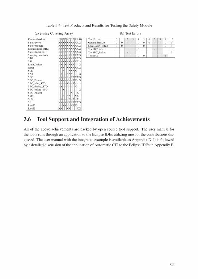
Table 3.4: Test Products and Results for Testing the Safety Module

(a) 2-wise Covering Array

Feature\Product 0 1 2 3 4 5 6 7 8 9 10

SafetyDrive XXXXXXXXXXX

SafetyModule XXXXXXXXXXX

CommunicationBus XXXXXXXXXXX

SafetyFunctions XXXXXXXXXXX

StoppingFunctions XXXXXXXXXXX

STO XXXXXXXXXXX

SS1 - - XX - X - XXX -

Limit_Values - X - X - XXX - - X

Other - XX - XXXXXXX

SSE - - X - - XXXX - -

SAR - X - - XXX - - - X

SBC - XX - X - XXXXX

SBC_Present - XX - X - - XX - X

SBC_after_STO - - - - X - - X - - -

SBC_during_STO - X - - - - - - X - -

SBC_before_STO - - X - - - - - - - X

SBC_Absent - - - - - - X - - X -

SMS - - X - XX - - XX -

SLS - XX - - X - X - X -

SIL XXXXXXXXXXX

Level2 - - XX - - XXX - -

Level3 XX - - XX - - - XX

(b) Test Errors

Test\Product 0 1 2 3 4 5 6 7 8 9 10

GeneralStartUp 0 0 - - 0 0 0 - - 0 0

Level3StartUpTest 0 0 0 0 0 0

TestSBC_After 0 -

TestSBC_Before - 0

TestSMS - 0 0 - 1

3.6 Tool Support and Integration of Achievements

All of the above achievements are backed by open source tool support. The user manual for

the tools runs through an application to the Eclipse IDEs utilizing most of the contributions dis-

cussed. The user manual with the integrated example is available as Appendix D. It is followed

by a detailed discussion of the application of Automatic CIT to the Eclipse IDEs in Appendix E.

65

Chapter 4

Discussion

This chapter first discusses threats to validity for the contributions in this thesis (Section 4.1)

and then discusses potentials and ideas for future work (Section 4.2).

4.1 Limitations and Threats to Validity

The following four subsections include threats to validity for the contributions. It also covers

threats to validity from the perspective of product line testing as a whole.

Generation of Covering Arrays from Large Feature Models

The ICPL algorithm was a major result of Paper 1 and 2. Several threats to validity can be

noted for these two papers: ICPL was evaluated by a comparison with three other algorithms for

covering array generation. The authors of ICPL are also those who performed the comparison

with the other algorithms. Below we discuss things that might have influenced the result of the

comparison as presented in Paper 2.

• Corpus Selection – The feature model corpus consists of feature models not made by

those who wrote or contributed to the contributions of this thesis. They are all used as

originals except for some minor changes: e.g. slight changes to the IDs due to differences

in what characters an ID can consist of.

ICPL was tuned to perform well on the corpus, while the other algorithms were presum-

ably developed without knowledge of these particular models. It would have been better

to compare all algorithms of a set of feature models none of the developers knew about

in advance.

• Corpus Completeness – No feature models were excluded from the corpus except for

their lack of realism. All feature models the authors were aware of and could verify

the origin of were included in the corpus within the time available for conducting the

experiment.

It is a possibility that the measurements are different given a more extensive corpus. A

more extensive corpus might be required to be representative of realistic feature models

in general.

67

• Adaptors – Some of the tools came with limited documentation. The adaptors that con-

vert from the three formats of feature models in our corpus to input for each of the three

other algorithms were written for the experiment in Paper 2 and are available as open

source. The results produced by each algorithm were confirmed to be complete and valid

by the same, separate algorithms.

It is, however, possible that the adaptors are unfair to the other algorithms, and that the

algorithms would have performed better with more suited converters. Had they been

available from the implementations, they would have been used instead.

• Other Algorithms – There are other algorithms that were not included in the comparison.

This issue was discussed in Section 2.4.4.

• Other Values of t – Empirics were not collected for t-wise testing of t >= 4. One of the

reasons for this is that the sizes of the covering arrays, using any algorithm, then becomes

significantly larger than the number of features in the feature model from which it is

generated. A second reason is that empirics indicate that 95% of bugs can be attributed to

the interaction of 3 features [94]. If the quality requirements are above this level, it is not

yet established that combinatorial interaction testing is the approach that should be taken

in the first place.

Optimized Testing in the Presence of Homogeneous AbstractionLayers

What are the liabilities in applying our techniques for reapplying test suites for products of a

covering array that differ only in the implementation of homogeneous abstraction layers?

• The solution does not make sense if the abstraction layer contains the union of function-

ality of the implementations. The intersection has to be considerable in order for the

application of this technique to pay off.

• The abstraction layer cannot be too general. For example, the team provider functionality

in Eclipse has multiple implementations: CVS, SVN, git, etc, but the functionality the

implementations offer is different. Thus, one have to supply one test suite per provider,

and that is also what is done in the Eclipse project.

• If one decides to make available implementation-specific behavior in the abstraction layer,

then the benefits of the pattern no longer applies, and one will have to significantly change

the test suites.

• Even though the test cases might be the same for all implementations, the initializations

of the test suites might be different.

Market-Focused Testing based on Weighted Sub-Product LineModels

A discussion of the limitations and threats to validity were not included in Paper 4 due to space

constraints.

68

• Partial Coverage – The theory of combinatorial interaction testing deals with the benefit

of 100% coverage. If a certain 95% 3-wise coverage is a 100% 2-wise coverage, does it

then have the bug-detection capabilities of 3-wise testing, or just that of 2-wise testing?

TOMRA wanted an answer to this question during our cooperation, but, unfortunately,

we were unable to offer any answer to this. This is a question for future work.

• Better than Manual Configuration by Domain Experts – One of our findings in the

experiments done at TOMRAwas that the manually configured products were quite good.

If this is the case, then why do we need theory and automation for doing what they

already accomplish manually? Indeed, maintaining the feature model and the weighted

sub-product line models are not free. Thus, even though the algorithms are fast once these

models are up-to-date, the task of maintaining them might be slower than just manually

updating the test lab by hand.

• Inflexibility – Configuring products by hand has a lot of flexibility. The domain experts

can choose to focus on whatever factors they want. They can react to new requirements

quickly. A fixed algorithm such as those related to the weighted sub-product line models

might not cater for any need they might have. This inflexibility might be a sign the theory

is not comprehensive enough yet and thus not ready for production.

• Difficulty – Understanding the theory of combinatorial interaction testing is not difficult;

however, it does require at least some days of training. This must be recognized by anyone

who will work with or think about it. This is in contrast with the apparent simplicity of

the covering arrays. They are seemingly just a handful of products. The computational

power required to generate them, however; is testament to the complexity that is packed

into those simple results.

Agile and Automatic Product Line Testing

Automatic CIT was never meant to be a final solution for product line testing but rather a com-

plete technique that could form the basis of further improvements or the basis of comparison.

These are some possible issues with the technique as proposed by us:

• Feature Interactions – Feature interactions are behavior that is caused by the combi-

nation of two or more features. Our technique does not specifically test that a feature

interaction between t features (for t-wise testing) interacts correctly with even more fea-

tures.

• Manual Hardware Product Lines – Product line engineering is also used for hardware

systems. Combinatorial interaction testing is also a useful technique to use for these

products lines; however, Automatic CIT is not fully automatic when the products must be

set up manually.

• Quality of the Automatic Tests – The quality of the results of the technique is dependent

on the quality of the automatic tests that are run for the features of the products.

• Feature Interaction Testing – A problem within the field of feature interaction testing

is how to best create tests as to identify interaction faults that occur between two or more

concrete features, the feature interaction problem [20]. Although an important problem,

it is not what our technique is for. Our technique covers all simple interactions and gives

insight into how they work together.

69

4.2 Future Work

4.2.1 Empirical Investigations

Empirical investigations were important for the contributions of this thesis. The work by Kuhn

et al. 2004 [94] form the basis for the arguments in favor of combinatorial interaction testing.

Their investigations are, however, not primarily targeted towards product line testing. Further

work on such empirical investigations has been carried out by Garvin and Cohen 2011 [59] and

Steffens et al. 2012 [146].

The three largest feature models in our collection were presented in and provided by She et

al. 2011 [141]. Their extraction of these feature models provided the basis for the development

of ICPL.

Tartler et al. 2011 [154] and related publications have done interesting experiments on

static analysis and testing of the Linux Kernel that have resulted in identifications of serious

bugs latent in some configurations.

Empirical studies of open source products lines by Berger et al. 2012 [13] show that many

open source product lines are developed using Kconfig. They note that "Kconfig models are

distributed over multiple files, organized according to the source code hierarchy." This aspect is

not usually incorporated into variability models from research.

Our industrial partners were surprised to be confronted with the claim that because they

have a product line, they must also have a problem with faults popping up when a new product

is configured. They did not experience this as a serious problem; they were not convinced that

a lot of effort was needed.

Now, the reason for this might be that they were unaware of the relation between a fault and

product line engineering—that a fault was due to the new configuration triggering some latent

fault. They might have thought that the fault is an ordinary fault and not a member of some new

category of faults caused by the new factors introduced with product line engineering. Indeed,

neither of the companies or the open-source case study describe their development practice as

product line engineering although that certainly is what they are doing.

Further technical advancements in the theory of product line testing depends on what is

found in the empirical investigations, as there is still significantly more to be learned from

them.

For example, an empirical investigation of latent faults in product lines would be valuable.

Such an investigation could either tell us that such faults are actually not a problem, or they

would give us a solid argument as to why product line testing is worthy of industrial attention.

Our industrial experiences gave us a clue that the actuality might be closer towards the former

than currently thought.

4.2.2 Complex Product Lines

Simple product lines are configured by a single feature model, its products are distributed evenly

around its configuration space, and the building of the products is done automatically by a click

of a button. A complex product line, in this context, means a product line with additional

challenges beyond such simple product lines. These complexities are such that techniques de-

70

veloped for the simple product line might not address the complexities in a suitable manner.

Mixed Hardware and Software Product Lines

TOMRA’s product line of RVMs is a good example of a product line with both hardware and

software variability. In our work with TOMRA, we focused on the hardware variability. The

products of hardware product lines are naturally more difficult to build automatically: The

assembly might require heavy-duty tools and expertise, or expensive robots. However, the

software variability, although linked with the hardware variability, is easy to automatically build

using software tools.

Whereas hardware often requires slowmanual tests to be performed, software can be quickly

tested.

The basic question here is how to balance the hardware and software testing to maximize

the fault-detection of the testing effort?

In addition, a single, fixed hardware configuration can still have its software configuration

automatically reconfigured. This brings up interesting questions in regards to covering array

generation optimized to respect this possibility.

Mixed-Variability Systems

Another kind of concern is a product line of which only a few products configured and sold,

but that still leaves a wide range of configurability for the customer or user. This lessens the

product line developers’ ability to check or know about any particular configuration. It actually

becomes more important to exercise the user-variability, while at the same it might seem less

important because only a few products are configured and sold by the developer.

In these cases, variability must be classified as more or less prone to being configured,

something that is not possible to specify using today’s feature models.

High Commonality, Few Products

Some product lines have a certain characteristic: They have a variability model, the products

have a high degree of commonality and there is a huge configuration space; yet, due to the

market situation and the nature of the product line, only a few products are configured and

available for purchase. The company derives benefits from using product line engineering, but,

when they have tested their (say six) products, they have tested every product they will sell for

the foreseeable future.

In these situations, combinatorial interaction testing does not make sense. The technique

derives it benefit from exercising every simple interaction. This is a waste if most of them will

never be used. Still, because of the high degree of commonality, it is wasteful to test every

system independently from scratch.

There should be a term to differentiate these kinds of product lines. We suggest highly,moderately and sparsely realized product lines, for lower degrees of realization, respectively.

Thus, we can ask the question: How should sparsely realized product lines be tested? Is it

essentially different from testing highly realized product lines? Are there special techniques for

each degree of realization?

71

Optimized Distribution of Test Cases

In our work on automatically testing the Eclipse IDEs or ABB’s Safety Modules, we assumed

that all test cases should be executed when they exercise relevant functionality in a product.

This might, however, be wasteful. This is especially a concern when manual testing is done.

The basic question is: Given that a test case exercises a set of functionality, on which prod-

ucts of a covering array should the test be performed, or, maybe more importantly, where should

they not be performed?

4.2.3 Product Line Engineering

Some opportunities for future work relate to product line engineering. These are opportunities

that are linked to novelties and technologies in product line engineering as such that might

benefit testing.

Distributed Variability Specifications

The Eclipse Project does not model their variability in a centralized way with a single feature

model; they primarily model their variability with distributed fragments throughout the system.

They do, however, for the purpose of automatic building, extract what is essentially a feature

model from the distributed fragments.

This is also observed in the Linux kernel project and in eCos. In both cases, the variability

of a component or a package is specified locally to that component or in that package.

Is testing systems with a distributed variability specification essentially different from test-

ing systems with a centralized variability specification? Are there special properties that can be

exploited in either?

One particular thing that is made easy using distributed variability specifications is depen-

dencies on components within a range of versions. This is difficult in basic feature models

because it would quickly bloat the model making it difficult to make out what it visualizes.

This is commonly solved in, for example, the Eclipse variability specifications by having the

variability specifications of each version separately specified.

Utilizing Implementation Information

A basic feature model is a simple model, and that has its benefit. It is essentialized, captures

variability information and is easy to work with using SAT-solvers and analyzers.

One way to keep feature models simple, but still enhance their powers, is to extract useful

information from the implementation of the product line. We explored one aspect of this in

our work on utilizing homogeneous abstraction layers. There we realized that some alternative

features are alternative because of the presence of a homogeneous abstraction layer. This was

then further used in generating covering arrays and testing the products in it.

We suspect, however, that there are more such things that can be exploited.

Variability models such as CVL, delta-oriented programming and delta modeling can spec-

ify variability on a very fine level of granularity. Variability realization using preprocessors are

72

popular for the Linux kernel and other open source systems. Can these fine-grained, or other

coarse-grained variability realizations, give us additional power when testing?

If such things are not automatically found, maybe they can be annotated on the feature

models directly by the designers of the product line? In our work, we annotated basic feature

models with a "Homogeneous Abstraction Layer"-annotation. This annotation allows tool-

support for marking products that are the same except for the implementations of these layers.

Are there other such useful annotations that can give us further tool support for testing?

Design Principles and SPL Testing

Before it makes sense to do quality assurance, a product line must be well designed. A good

design is a way to avoid problems early in development. When this is in place, however, testing

can be used to validate the system further.

There are a wide range of design principles and patterns in software engineering literature.

Do some of these make the product line easier to test and validate? For example, the Wrapper-

Facade design pattern [138] encapsulates platform specific, non-object-oriented functionality

in a class. This is obviously useful to promote variability of a product line over a variety of

platforms. As a second example, the Release-Reuse Equivalency Principle [104] states that the

granule of reuse should be the granule of release. How does this apply in the context of product

line engineering? How does this level of granularity affect testing?

Questions such as these can be made for many of the relevant principles and patterns.

Exploiting Version Information

Dependencies in the Eclipse IDEs are not just to another feature but also to a range of feature

versions. Such versioned dependencies are difficult to model in a basic feature model and

difficult to graphically visualize.

More importantly however, how do the versions give us information about how to test the

system? Maintaining old versions are important for several reasons. A range of versions might

be installed in offline systems. In addition, older versions might need maintenance because

of customers who do not need or want to upgrade. As with homogeneous abstraction layers,

maybe they can be turned into an advantage?

4.2.4 Algorithms

The opportunities in this subsection are related to algorithmic challenges.

Further Improvements of ICPL

The ICPL algorithmwas a significant improvement over previous algorithms for t-wise covering

array generation. We did not, however, rule out further improvements. Can the algorithms be

parallelized further? Complete parallelization would enable large clusters to efficiently run it

without an upper bound. In addition, can the memory requirements due to the storage of all

t-sets be reduced? Is it possible not to store all t-sets? There are many possibilities for further

improvements of ICPL.

73

Upper bound for ICPL

Chvátal’s algorithm is a greedy approximation algorithm for a problem classified as NP-complete

by complexity analysis. A good upper bound was established in Chvátal 1979 [31]. This upper

bound does not apply for ICPL because not all possible configurations are browsed. Instead,

another greedy step is added to construct a single configuration. It would be interesting to know

what is the upper bound guarantee of ICPL (or a similar algorithm), or, alternatively, whether

ICPL can be modified to give it the upper bound guarantee of Chvátal’s algorithm.

Extracting Basic Feature Models

This thesis deals with basic feature models. There are other kinds of feature models with more

complex mechanisms. The work presented in this thesis still applies to more complex feature

modeling mechanisms. Many types of feature models are more complex than basic feature

models. Some promising techniques for testing product lines require a basic feature model;

thus, these techniques cannot be used if a product line is not modeled with a basic feature

model.

Many, more complex types of feature models have been proposed since the introduction of

the notion of a feature model. Many of the powerful mechanisms have been included in the

proposed standard variability language by the OMG, CVL [71]. This standard also introduces

additional complex mechanisms to model variability: non-Boolean Variability, non-Boolean

constraints, cardinality-based feature models [45], recursive variability, contextual constraints,

OCL Constraints, etc.

Enabling the extraction of a basic feature model from a more complex type of feature model

for the purpose of testing would be an interesting topic. This could be both manual and auto-

matic methods to be done by a test engineer. A solution would enable the application of some

promising techniques for testing product lines when a product line is modeled using a more

complex type of feature model. The test engineer may, however, in some situations, have to

conclude that extracting a basic feature model for the purpose of testing is simply not purpose-

ful.

Evolving Covering Arrays

When a software product line evolves, the products of an old covering array might no longer

cover the simple interactions of the product line. Thus, a new test suite must be generated.

Currently, no algorithm exists for minimizing the difference between the old and new test prod-

ucts, causing the new test suite to be unnecessarily different from the old test suite. This causes

unnecessary effort in co-evolving a test suite with an evolving product line.

It would be good to have an efficient algorithm for incremental evolution of test products

with an evolving product line. This would reduce effort in maintaining a test suite when a prod-

uct line evolves. The efficiency could be demonstrated with an experiment on realistic feature

models that were realistically evolved. Well-documented evolutions exist for, for example, the

Linux kernel and the Eclipse IDEs.

74

4.2.5 Engineering

These opportunities are not so much related to novel research, but might spawn some inter-

esting research challenges that need solving. At the face of it, these challenges are currently

demanding engineering tasks.

Using Virtual Machines

While the testing of a system running on a single platform can be carried out on that platform,

testing systems for various platforms in a uniform and automatic way cannot be done easily on

a single platform. Today, good virtual machine technology exists. This enables the execution

and control of systems running in other operating systems and hardware architectures.

To fully test, for example, the Eclipse IDEs or the Linux kernel, a variety of virtual machines

could be automatically set up with the right configuration. Eclipse and Linux could then be

automatically installed on these virtual machines and tested.

Full Testing of the Eclipse IDEs

Setting up a full-scale production test of the Eclipse IDEs should be possible given the experi-

ments carried out in Paper 5 of this thesis. This requires some engineering work, some domain

experts, hardware or virtual machines.

We think that such an application would be an interesting case study from which we could

learn something about large-scale product line testing in practice.

It could also be a demonstration worth looking at for other developers of industrial product

lines for whether they should adapt such techniques for their product line. In the end, a demon-

stration that something actually works on a large-scale is an argument you cannot ignore.

75

Chapter 5

Conclusion

This chapter concludes Part I of the thesis by summarizing the results and their main evaluations.

5.1 Results

In this thesis, we contributed to the testing of product lines of industrial size by advancing

combinatorial interaction testing (CIT).

Existing applied techniques such as reusable component testing, does not exercise feature

interactions. There are many suggestions of how to test feature interactions. Based on the

background and related work, and taking into account the industrial case studies, combinatorial

interaction testing (CIT) emerged as the most promising approach. The primary reasons were

that 1) the technique does address the issue of interaction testing and 2) the technique can be

applied within the current work-flows established; it does not require a significant change in

development practices. This enables us to, for example, apply the technique of Contribution 5

to the entire part of the Eclipse IDE product line supported by the Eclipse project with a small

workforce.

Contribution 1 and 2 culminated in the ICPL algorithm. ICPL is a covering array genera-

tion algorithm that can generate covering arrays for the larger product lines. In particular, it was

the first algorithm to generate a pair-wise covering array for the Linux Kernel feature model,

one of the largest product lines whose feature model is available.

Having a scalable algorithm for covering array generation encourages further advancements

of combinatorial interaction testing for product lines. We contributed three advancements: Uti-

lization of homogeneous abstraction layers for oracles, market-focused CIT and automatic CIT.

Contribution 3: Many product lines utilize homogeneous abstraction layers to get a uni-

form interface to a multitude of similar systems. We showed how such layers could be exploited

to improve product line testing. In a covering array generated from a product line with such ab-

straction layers, test suites can be reused for products that differ only in the implementation

of one or more homogeneous abstraction layers. Further, these repeated executions of the test

suites allows for a voting oracle or taking one of the executions to be a gold standard oracle.

Contribution 4: Sub-product line models were contributed for modeling the market situa-

tion of a product line. Associated algorithms allow covering arrays to be adapted to, optimized

for and evolved with the market situation. The market situation can model the customer priority

77

or criticality. They can model the expectations and make testing of what will be the situation in

the future.

Contribution 5: The automatic CIT technique filled in what was missing to make CIT

automatic. Test for parts of a product line can be reused to test interaction among the features.

Rerunning existing tests on each applicable product of the covering array of a product line

does give us some insight into the simple interaction among the features. Such tests are often

developed for product lines and are thus readily available even for existing product lines. This

allowed us to, for example, apply the technique in full to the part of the Eclipse IDE product

line supported by the Eclipse project.

Tool support: Tools were implemented with the contributed algorithms and techniques.

These tools are available freely as open source under the EPL v1.0 license.

5.2 Evaluation

Contribution 1 and 2: The ICPL algorithm was evaluated by comparing it to three other al-

gorithms from the research community and one of our previous algorithms. The five algorithms

were executed on 19 existing, realistic feature models. The following was concluded from this

evaluation:

ICPL generates covering arrays of an acceptable size, comparable to other state of the art

algorithms. Even though it is non-deterministic, there is little to none variance between execu-

tions. It is faster than the other algorithms; for 2-wise testing, it was estimated to be 1,000 times

faster than the second fastest algorithm for an industrially sized feature model. In addition, al-

though MoSo-PoLiTe was the second fastest, its covering array sizes were larger than the other

algorithms. For 3-wise testing, ICPL was found to be almost 30,000 times faster than the second

fastest for a feature model of industrial size. Note that these factors grow as the feature model

gains more features; however, the example here is one of the largest known feature models.

The three advancements of CIT were evaluated by the application of them to four industrial

case studies; the open source system allowed us to document our results and provide repro-

ducible results.

Contribution 3: Two of our case studies had homogeneous abstraction layers with which

we could experiment with our related contribution. In the Finale case study, if we want to

exercise all pairs of interactions, all products containing a version of client-side Windows paired

with a version of an accounting system, then we need at least 6 ∗ 18 = 108 products. Indeed,

the pair-wise covering array contains 116 products. If we group together those products that

only differ below a homogeneous abstraction layer, we reduce the number to 60. Unfortunately,

details of this experiment are unavailable for documentation.

To provide a documented experiment, we did apply the technique to the Eclipse IDEs. In

total, they support 16 combinations of hardware, windowing systems and operating systems.

The pair-wise covering array of a certain sub-set of the Eclipse IDEs was 41 products. Out of

these, only 20 groups of products need to have unique test suites. Internally in the groups, the

products differ only beneath the homogeneous abstraction layers. Covering the system with

1-wise testing gives 10 products, but only 5 test suites are required. For 3-wise testing, with

119 configurations, only 45 test suites are required.

78

Contribution 4: The main experiment with weighted sub-product line models and associ-

ated algorithms was the TOMRA case study. This means that the experiments are not repro-

ducible. The feature model of the TOMRA case has 68 features (which yield 435,808 possible

configurations) TOMRA’s existing lab had 12 products manually configured by domain experts.

The experiments centered on these products. We found that: (1) The domain experts found that

covering arrays generated from the weighted models were more familiar to them and were

closer to products found in the market. (2) Their existing lab had higher weight coverage than

t-set coverage. (3) Significantly fewer products were needed than they currently had to achieve

the same weight coverage. (4) Finally, the domain experts found the suggestions given by the

incremental evolution algorithm to be good and relevant.

We supplemented this commercial case with an application to the Eclipse IDEs. It was

simpler, but it is at least documented openly and reproducibly. Based on download statistics

of the 12 Eclipse IDE products offered for download, we found that 4 products are needed to

achieve 95% weight coverage.

Contribution 5: The full Automatic CIT technique was applied to two industrial product

lines: First of all, it was applied to a simulated version of the ABB safety module. The feature

model had 22 features and yielded 640 possible products in the original experiment (512 in a

corrected version). Of these configurations, the pair-wise covering array consisted of 11 prod-

ucts that when tested with Automatic CIT produced five test failures. These failures revealed

two bugs as identified by the creators of the simulated version of the safety module.

Automatic CIT was also applied to the part of the Eclipse IDEs supported by the Eclipse

Project. This is one of the largest documented applications of a product line testing technique.

We created a feature model for the part of the Eclipse IDEs supported by the Eclipse Project.

The feature model consisted of 22 features. We implemented Automatic CIT for the Eclipse

Platform plug-in system, and we created a feature mapping for 36 existing test suites. This

experiment consisted of 40,744 tests and resulted in 417,293 test results. Out of these, 513

failures were produced that are probably caused by interaction faults.

79

Bibliography

[1] ABB. ABB industrial drives - Safety functions module for extending applica-

tion safety. http://www05.abb.com/global/scot/scot201.nsf/

veritydisplay/cff4a15410027401c1257aef003b7bc7/$file/

16645_FSO-11_flyer_EN_3AUA0000116739_RevB_lowres.pdf, 2013.

[2] Hiralal Agrawal, Joseph R. Horgan, Edward W. Krauser, and Saul London. Incremental

regression testing. In Proceedings of the Conference on Software Maintenance, ICSM

’93, pages 348–357, Washington, DC, USA, 1993. IEEE Computer Society.

[3] Sergej Alekseev, Rebecca Tiede, and Peter Tollkühn. Systematic approach for using

the classification tree method for testing complex software-systems. In Proceedings ofthe 25th conference on IASTED International Multi-Conference: Software Engineering,SE’07, pages 261–266, Anaheim, CA, USA, 2007. ACTA Press.

[4] Finale Systemer AS. Produktkatalog. http://www.finale.no/

produktkatalog.4828511-165509.html, 2013.

[5] Automated Combinatorial Testing for Software group at NIST, Arlington, Texas, US.

User Guide for ACTS, beta 2 - revision 1.5 edition, December 2011.

[6] J. Bach. Allpairs test case generation tool (version 1.2.1), May 2013.

[7] Don Batory. The design and implementation of hierarchical software systems with

reusable components. ACM Transactions on Software Engineering and Methodology,1:355–398, 1992.

[8] Don Batory, Peter Höfner, and Jongwook Kim. Feature interactions, products, and com-

position. SIGPLAN Not., 47(3):13–22, October 2011.

[9] Don Batory, Jacob N. Sarvela, Axel Rauschmayer, Student Member, and Student Mem-

ber. Scaling step-wise refinement. IEEE Transactions on Software Engineering, 30,2003.

[10] Don Batory, Jacob Neal Sarvela, and Axel Rauschmayer. Scaling step-wise refinement.

IEEE TRANSACTIONS ON SOFTWARE ENGINEERING, 30(6):2004, 2004.

[11] Don S. Batory. Feature models, grammars, and propositional formulas. In J. Henk Ob-

bink and Klaus Pohl, editors, SPLC, volume 3714 of Lecture Notes in Computer Science,pages 7–20. Springer, 2005.

81

[12] Kent Beck. Test Driven Development: By Example. Addison-Wesley Longman Publish-

ing Co., Inc., Boston, MA, USA, 2002.

[13] Thorsten Berger, Steven She, Rafael Lotufo, Andrzej Wasowski, and Krzysztof Czar-

necki. Variability modeling in the systems software domain. Technical Report GS-

DLAB–TR 2012–07–06, Generative Software Development Laboratory, University of

Waterloo, 2012. journal submission under review.

[14] Antonia Bertolino, Alessandro Fantechi, Stefania Gnesi, and Giuseppe Lami. Product

line use cases: Scenario-based specification and testing of requirements. In Käkölä and

Dueñas [90], pages 425–445.

[15] Antonia Bertolino and Stefania Gnesi. Use case-based testing of product lines. SIGSOFTSoftw. Eng. Notes, 28(5):355–358, 2003.

[16] Antonia Bertolino and Stefania Gnesi. Pluto: A test methodology for product families.

In van der Linden [162], pages 181–197.

[17] Armin Biere and Wolfgang Kunz. Sat and atpg: Boolean engines for formal hard-

ware verification. In Proceedings of the 2002 IEEE/ACM international conference onComputer-aided design, ICCAD ’02, pages 782–785, New York, NY, USA, 2002. ACM.

[18] Robert V. Binder. Testing object-oriented systems: models, patterns, and tools. Addison-

Wesley Longman Publishing Co., Inc., Boston, MA, USA, 1999.

[19] Jan Bosch and Jaejoon Lee, editors. Software Product Lines: Going Beyond - 14thInternational Conference, SPLC 2010, Jeju Island, South Korea, September 13-17, 2010.Proceedings, volume 6287 of Lecture Notes in Computer Science. Springer, 2010.

[20] T.F. Bowen, FS Dworack, C.H. Chow, N. Griffeth, G.E. Herman, and Y.J. Lin. The fea-

ture interaction problem in telecommunications systems. In Software Engineering forTelecommunication Switching Systems, 1989. SETSS 89., Seventh International Confer-ence on, pages 59–62. IET, 1989.

[21] Renée C. Bryce and Charles J. Colbourn. Prioritized interaction testing for pair-wise

coverage with seeding and constraints. Information and Software Technology, 48(10):960– 970, 2006. Advances in Model-based Testing.

[22] Isis Cabral, Myra B. Cohen, and Gregg Rothermel. Improving the testing and testability

of software product lines. In Bosch and Lee [19], pages 241–255.

[23] Andrea Calvagna and Angelo Gargantini. A logic-based approach to combinatorial test-

ing with constraints. In Bernhard Beckert and Reiner Hähnle, editors, Tests and Proofs,volume 4966 of Lecture Notes in Computer Science, pages 66–83. Springer Berlin / Hei-

delberg, 2008. 10.1007/978-3-540-79124-9_6.

[24] Andrea Calvagna and Angelo Gargantini. Combining satisfiability solving and heuris-

tics to constrained combinatorial interaction testing. In Catherine Dubois, editor, Testsand Proofs, volume 5668 of Lecture Notes in Computer Science, pages 27–42. SpringerBerlin / Heidelberg, 2009.

82

[25] Andrea Calvagna and Angelo Gargantini. Ipo-s: Incremental generation of combinatorial

interaction test data based on symmetries of covering arrays. Software Testing Verifica-tion and Validation Workshop, IEEE International Conference on, 0:10–18, 2009.

[26] Andrea Calvagna and Angelo Gargantini. A formal logic approach to constrained combi-

natorial testing. Journal of Automated Reasoning, 45:331–358, 2010. 10.1007/s10817-

010-9171-4.

[27] Andrea Calvagna, Angelo Gargantini, and Paolo Vavassori. Combinatorial interaction

testing with citlab. In Sixth IEEE International Conference on Software Testing, Verifi-cation and Validation, Proceedings of, 2013.

[28] Andrea Calvagna, Angelo Gargantini, and Paolo Vavassori. Combinatorial testing for

feature models using citlab. In The 2nd International Workshop on Combinatorial Testing(IWCT 2013), Proceedings of, 2013.

[29] Andrea Calvagna, Giuseppe Pappalardo, and Emiliano Tramontana. A novel approach

to effective parallel computing of t-wise covering arrays. In Proceedings of the 2012IEEE 21st International Workshop on Enabling Technologies: Infrastructure for Collab-orative Enterprises, WETICE ’12, pages 149–153, Washington, DC, USA, 2012. IEEE

Computer Society.

[30] Philip Chong and Mukul Prasad. Satisfiability for atpg: Is it easy?, 1998.

[31] Václav Chvátal. A greedy heuristic for the Set-Covering problem. Mathematics of Op-erations Research, 4(3):233–235, 1979.

[32] Harald Cichos, Sebastian Oster, Malte Lochau, and Andy Schürr. Model-based coverage-

driven test suite generation for software product lines. In Proceedings of the 14th inter-national conference on Model driven engineering languages and systems, MODELS’11,

pages 425–439, Berlin, Heidelberg, 2011. Springer-Verlag.

[33] Dave Clarke, Michiel Helvensteijn, and Ina Schaefer. Abstract delta modeling. SIGPLANNot., 46(2):13–22, October 2010.

[34] Alistair Cockburn. Writing Effective Use Cases. Addison-Wesley Professional, January

2000.

[35] D. M. Cohen, S. R. Dalal, A. Kajla, and G. C. Patton. The automatic efficient tests

generator. In Fifth IEEE International Symposium on Software Reliability Engineering,Proceedings of, page 303–309, 1994.

[36] David Cohen, Ieee Computer Society, Siddhartha R. Dalal, Michael L. Fredman, and

Gardner C. Patton. The aetg system: An approach to testing based on combinatorial

design. IEEE Transactions on Software Engineering, 23:437–444, 1997.

[37] David M. Cohen, Siddhartha R. Dalal, Jesse Parelius, and Gardner C. Patton. The combi-

natorial design approach to automatic test generation. IEEE Softw., 13(5):83–88, Septem-

ber 1996.

83

[38] Myra B. Cohen. Designing test suites for software interaction testing. PhD thesis, The

University of Auckland, 2004.

[39] Myra B. Cohen, Charles J. Colbourn, and Alan C. H. Ling. Augmenting simulated

annealing to build interaction test suites. In Proceedings of the 14th International Sym-posium on Software Reliability Engineering, ISSRE ’03, pages 394–, Washington, DC,

USA, 2003. IEEE Computer Society.

[40] Myra B. Cohen, Matthew B. Dwyer, and Jiangfan Shi. Coverage and adequacy in soft-

ware product line testing. In ROSATEA ’06: Proceedings of the ISSTA 2006 workshopon Role of software architecture for testing and analysis, pages 53–63, New York, NY,

USA, 2006. ACM.

[41] Myra B. Cohen, Matthew B. Dwyer, and Jiangfan Shi. Interaction testing of highly-

configurable systems in the presence of constraints. In ISSTA ’07: Proceedings of the2007 international symposium on Software testing and analysis, pages 129–139, New

York, NY, USA, 2007. ACM.

[42] Myra B. Cohen, Matthew B. Dwyer, and Jiangfan Shi. Constructing interaction test suites

for highly-configurable systems in the presence of constraints: A greedy approach. IEEETransactions on Software Engineering, 34:633–650, 2008.

[43] Myra B. Cohen, Peter B. Gibbons, Warwick B. Mugridge, and Charles J. Colbourn.

Constructing test suites for interaction testing. In Lori A. Clarke, Laurie Dillon, and

Walter F. Tichy, editors, ICSE, pages 38–48. IEEE Computer Society, 2003.

[44] Charles J. Colbourn and Myra B. Cohen. A deterministic density algorithm for pairwise

interaction coverage. In Proc. of the IASTED Intl. Conference on Software Engineering,pages 242–252, 2004.

[45] Krzysztof Czarnecki, Simon Helsen, and Ulrich W. Eisenecker. Formalizing cardinality-

based feature models and their specialization. Software Process: Improvement and Prac-tice, 10(1):7–29, 2005.

[46] Jacek Czerwonka. Pairwise testing in real world. In Proceedings of 24th Pacific North-west Software Quality Conference, 2006, 2006.

[47] Leonardo Mendonça de Moura, Sam Owre, Harald Rueß, John M. Rushby, Natarajan

Shankar, Maria Sorea, and Ashish Tiwari. Sal 2. In Rajeev Alur and Doron Peled, editors,

CAV, volume 3114 of Lecture Notes in Computer Science, pages 496–500. Springer,

2004.

[48] DIMACS. Satisfiability Suggested Format. Technical report, Center for Discrete Math-

ematics and Theoretical Computer Science, 1993.

[49] Michael Dukaczewski, Ina Schaefer, Remo Lachmann, and Malte Lochau.

Requirements-based delta-oriented spl testing. In Product Line Approaches in SoftwareEngineering (PLEASE), 2013 4th International Workshop on, 2013.

84

[50] Emelie Engström, Per Runeson, and Mats Skoglund. A systematic review on regression

test selection techniques. Inf. Softw. Technol., 52(1):14–30, January 2010.

[51] Erich Gamma. How (7 years of) eclipse changed my views on software de-

velopment. http://qconlondon.com/dl/qcon-london-2008/slides/

ErichGamma_qcon2008.pdf, 2008.

[52] Erich Gamma, Richard Helm, Ralph E. Johnson, and John Vlissides. Design Patterns:Elements of Reusable Object-Oriented Software. Addison-Wesley, Reading, MA, 1995.

[53] DharmalingamGanesan, Jens Knodel, Ronny Kolb, Uwe Haury, and GeraldMeier. Com-

paring costs and benefits of different test strategies for a software product line: A study

from testo ag. In Proceedings of the 11th International Software Product Line Confer-ence, pages 74–83, Washington, DC, USA, 2007. IEEE Computer Society.

[54] Dharmalingam Ganesan, Mikael Lindvall, David McComas, Maureen Bartholomew,

Steve Slegel, Barbara Medina, Rene Krikhaar, and Chris Verhoef. An analysis of unit

tests of a flight software product line. Science of Computer Programming, 2012.

[55] Michael R. Garey and David S. Johnson. Computers and Intractability; A Guide to theTheory of NP-Completeness. W. H. Freeman & Co., New York, NY, USA, 1990.

[56] Angelo Gargantini and Paolo Vavassori. Citlab: A laboratory for combinatorial interac-

tion testing. In Proceedings of the 2012 IEEE Fifth International Conference on SoftwareTesting, Verification and Validation, ICST ’12, pages 559–568, Washington, DC, USA,

2012. IEEE Computer Society.

[57] Brady J. Garvin and Myra B. Cohen. Feature interaction faults revisited: An exploratory

study. In Proceedings of the 22nd International Symposium on Software Reliability En-gineering (ISSRE 2011), November 2011.

[58] Brady J. Garvin, Myra B. Cohen, and Matthew B. Dwyer. An improved meta-heuristic

search for constrained interaction testing. Search Based Software Engineering, Interna-tional Symposium on, 0:13–22, 2009.

[59] Brady J. Garvin, Myra B. Cohen, and Matthew B. Dwyer. Evaluating improvements

to a meta-heuristic search for constrained interaction testing. Empirical Softw. Engg.,16:61–102, February 2011.

[60] Hassan Gomaa. Designing software product lines with UML - from use cases to pattern-based software architectures. ACM, 2005.

[61] Wolfgang Grieskamp, Xiao Qu, Xiangjun Wei, Nicolas Kicillof, and Myra Cohen. Inter-

action coverage meets path coverage by smt constraint solving. In Manuel Núñez, Paul

Baker, and Mercedes Merayo, editors, Testing of Software and Communication Systems,volume 5826 of Lecture Notes in Computer Science, pages 97–112. Springer Berlin /

Heidelberg, 2009.

85

[62] Matthias Grochtmann and Klaus Grimm. Classification trees for partition testing. Soft-ware Testing, Verification and Reliability, 3(2):63–82, 1993.

[63] O. Gruber, BJ Hargrave, J. McAffer, P. Rapicault, and T. Watson. The eclipse 3.0 plat-

form: adopting osgi technology. IBM Systems Journal, 44(2):289–299, 2005.

[64] Arne Haber, Holger Rendel, Bernhard Rumpe, and Ina Schaefer. Delta modeling for

software architectures. In In MBEES, 2011.

[65] R. M. Haralick and G. L. Elliott. Increasing tree search efficiency for constraint satisfac-

tion problems. Artificial Intelligence, 14:263–313, 1980.

[66] Alan Hartman. Software and hardware testing using combinatorial covering suites. In

MartinCharles Golumbic and IrithBen-Arroyo Hartman, editors, Graph Theory, Com-binatorics and Algorithms, volume 34 of Operations Research/Computer Science Inter-faces Series, pages 237–266. Springer US, 2005.

[67] Jean Hartmann, Marlon Vieira, and Axel Ruder. A UML-based approach for validating

product lines. In Birgit Geppert, Charles Krueger, and Jenny Li, editors, Proceedingsof the International Workshop on Software Product Line Testing (SPLiT 2004), pages58–65, Boston, MA, August 2004.

[68] Evelyn Nicole Haslinger, Roberto E. Lopez-Herrejon, and Alexander Egyed. Using fea-

ture model knowledge to speed up the generation of covering arrays. In Proceedingsof the Seventh International Workshop on Variability Modelling of Software-intensiveSystems, VaMoS ’13, pages 16:1–16:6, New York, NY, USA, 2013. ACM.

[69] Øystein Haugen, Birger Møller-Pedersen, Jon Oldevik, Gøran K. Olsen, and Andreas

Svendsen. Adding standardized variability to domain specific languages. In SPLC ’08:Proceedings of the 2008 12th International Software Product Line Conference, pages139–148, Washington, DC, USA, 2008. IEEE Computer Society.

[70] Øystein Haugen and Birger Møller-Pedersen. Javaframe: Framework for java-enabled

modelling. In Proceedings of Ericsson Conference on Software Engineering, 2000.

[71] Øystein Haugen et al. Common Variability Language (CVL)—OMG

Revised Submission, August 2012. http://www.omgwiki.org/

variability/lib/exe/fetch.php?id=start&cache=cache&media=

cvl-revised-submission.pdf.

[72] Christopher Henard, Mike Papadakis, Gilles Perrouin, Jacques Klein, Patrick Heymans,

and Yves Le Traon. Bypassing the combinatorial explosion: Using similarity to generate

and prioritize t-wise test suites for large software product lines. CoRR, abs/1211.5451,2012.

[73] A. Hervieu, B. Baudry, and A. Gotlieb. Pacogen: Automatic generation of pairwise test

configurations from feature models. In Software Reliability Engineering (ISSRE), 2011IEEE 22nd International Symposium on, pages 120–129. IEEE, 2011.

86

[74] IEEE. IEEE 90: IEEE Standard Glossary of Software Engineering Terminology. IEEE,1990.

[75] Daniel Jackson. Alloy: a lightweight object modelling notation. ACM Trans. Softw. Eng.Methodol., 11(2):256–290, April 2002.

[76] Bob Jenkins. jenny: a pairwise testing tool, May 2013.

[77] Martin Fagereng Johansen, Øystein Haugen, and Franck Fleurey. A Survey of Empirics

of Strategies for Software Product Line Testing. In Lisa O’Conner, editor, Proceedingsof the 2011 IEEE Fourth International Conference on Software Testing, Verification andValidation Workshops, ICSTW ’11, pages 266–269, Washington, DC, USA, 2011. IEEE

Computer Society.

[78] Martin Fagereng Johansen, Øystein Haugen, and Franck Fleurey. Properties of realistic

feature models make combinatorial testing of product lines feasible. In Jon Whittle,

Tony Clark, and Thomas Kuehne, editors, Proceedings of Model Driven EngineeringLanguages and Systems, 14th International Conference, MODELS 2011, pages 638–652,Wellington, New Zealand, October 2011. Springer, Heidelberg.

[79] Martin Fagereng Johansen, Øystein Haugen, and Franck Fleurey. An Algorithm for Gen-

erating t-wise Covering Arrays from Large Feature Models. In Vander Alves and Andre

Santos, editors, Proceedings of the 16th International Software Product Line Conference(SPLC 2012). ACM, 2012.

[80] Martin Fagereng Johansen, Øystein Haugen, and Franck Fleurey. Bow Tie Testing - A

Testing Pattern for Product Lines. In Paris Avgeriou, editor, Proceedings of the 16thAnnual European Conference on Pattern Languages of Programming (EuroPLoP 2011).ACM, 2012.

[81] Martin Fagereng Johansen, Øystein Haugen, Franck Fleurey, Erik Carlson, Jan Endresen,

and Tormod Wien. A Technique for Agile and Automatic Interaction Testing for Prod-

uct Lines. In Brian Nielsen and Carsten Weise, editors, Proceedings of The 23rd IFIPInternational Conference on Testing Software and Systems (ICTSS’12), pages 39–54.

Springer, 2012.

[82] Martin Fagereng Johansen, Øystein Haugen, Franck Fleurey, Anne Grete Eldegard, and

Torbjørn Syversen. Generating Better Partial Covering Arrays by Modeling Weights on

Sub-Product Lines. In Robert France, Juergen Kazmeier, Colin Atkinson, and Ruth Breu,

editors, Proceedings of Model Driven Engineering Languages and Systems, 15th Inter-national Conference, MODELS 2012, Innsbruck, Austria, September 2012. Springer.

[83] Paul C. Jorgensen. Software Testing: A Craftsman’s Approach, Third Edition. AUER-

BACH, 3 edition, 2008.

[84] Erik Kamsties, Klaus Pohl, Sacha Reis, and Andreas Reuys. Testing variabilities in use

case models. In van der Linden [162], pages 6–18.

87

[85] Erik Kamsties, Klaus Pohl, and Andreas Reuys. Supporting test case derivation in do-

main engineering. In Proceedings of the Seventh World Conference on Integrated Designand Process Technology (IDPT-2003). Society for Design and Process Science (SDPS),

2003.

[86] K. C. Kang, S. G. Cohen, J. A. Hess, W. E. Novak, and A. S. Peterson. Feature-oriented

domain analysis (foda) feasibility study. Technical report, Carnegie-Mellon University

Software Engineering Institute, November 1990.

[87] Christian Kästner, Sven Apel, Syed Saif ur Rahman, Marko Rosenmüller, Don Batory,

and Gunter Saake. On the impact of the optional feature problem: analysis and case

studies. In Proceedings of the 13th International Software Product Line Conference,SPLC ’09, pages 181–190, Pittsburgh, PA, USA, 2009. Carnegie Mellon University.

[88] Gregor Kiczales, John Lamping, Anurag Mendhekar, Chris Maeda, Cristina Lopes, Jean-

Marc Loingtier, and John Irwin. Aspect-oriented programming. Springer, 1997.

[89] Chang Hwan Peter Kim, Don S. Batory, and Sarfraz Khurshid. Reducing combinatorics

in testing product lines. In Proceedings of the tenth international conference on Aspect-oriented software development, AOSD ’11, pages 57–68, New York, NY, USA, 2011.

ACM.

[90] Timo Käkölä and Juan C. Dueñas, editors. Software Product Lines - Research Issues inEngineering and Management. Springer, Berlin, Heidelberg, 2006.

[91] Mohammad F. J. Klaib, Kamal Zuhairi Zamli, Nor Ashidi Mat Isa, Mohammed I. Younis,

and Rusli Abdullah. G2way a backtracking strategy for pairwise test data generation. In

APSEC, pages 463–470. IEEE, 2008.

[92] Ronny Kolb. A risk-driven approach for efficiently testing software product lines.

In Net.ObjectDays 2003. Workshops. Industriebeiträge - Tagungsband : OffizielleNachfolge-Veranstaltung der JavaDays, STJA, JIT, DJEK, pages 409—-414, 2003.

[93] Matthias Kowal, Sandro Schulze, and Ina Schaefer. Towards efficient spl testing by

variant reduction. In Proceedings of the 4th international workshop on Variability &composition, VariComp ’13, pages 1–6, New York, NY, USA, 2013. ACM.

[94] D. Richard Kuhn, Dolores R. Wallace, and Albert M. Gallo. Software fault interac-

tions and implications for software testing. IEEE Transactions on Software Engineering,30(6):418–421, 2004.

[95] Sean Quan Lau. Domain analysis of e-commerce systems using feature-based model

templates. Master’s thesis, ECE Department, University of Waterloo, Canada, 2006.

[96] Y. Lei, R. Kacker, D.R. Kuhn, V. Okun, and J. Lawrence. Ipog: A general strategy for t-

way software testing. In Engineering of Computer-Based Systems, 2007. ECBS’07. 14thAnnual IEEE International Conference and Workshops on the, pages 549–556. IEEE,

2007.

88

[97] Yu Lei, Raghu Kacker, D. Richard Kuhn, Vadim Okun, and James Lawrence. Ipog-ipog-

d: efficient test generation for multi-way combinatorial testing. Softw. Test. Verif. Reliab.,18(3):125–148, September 2008.

[98] Yu Lei and Kuo-Chung Tai. In-parameter-order: A test generation strategy for pairwise

testing. In The 3rd IEEE International Symposium on High-Assurance Systems Engineer-ing, HASE ’98, pages 254–261, Washington, DC, USA, 1998. IEEE Computer Society.

[99] Jörg Liebig, Alexander von Rhein, Christian Kästner, Sven Apel, Jens Dörre, and Chris-

tian Lengauer. Scalable analysis of variable software. In Proceedings of the EuropeanSoftware Engineering Conference and ACM SIGSOFT Symposium on the Foundations ofSoftware Engineering (ESEC/FSE), New York, NY, 8 2013. to appear; accepted 30 May

2013.

[100] S. Lity, M. Lochau, I. Schaefer, and U. Goltz. Delta-oriented model-based spl regres-

sion testing. In Product Line Approaches in Software Engineering (PLEASE), 2012 3rdInternational Workshop on, pages 53–56, 2012.

[101] Jia Liu, Don Batory, and Christian Lengauer. Feature oriented refactoring of legacy ap-

plications. In Proceedings of the 28th international conference on Software engineering,ICSE ’06, pages 112–121, New York, NY, USA, 2006. ACM.

[102] Malte Lochau, Ina Schaefer, Jochen Kamischke, and Sascha Lity. Incremental model-

based testing of delta-oriented software product lines. In Achim D. Brucker and Jacques

Julliand, editors, TAP, volume 7305 of Lecture Notes in Computer Science, pages 67–82.Springer, 2012.

[103] Roberto E. Lopez-herrejon and Don Batory. A standard problem for evaluating product-

line methodologies. In Proc. 2001 Conf. Generative and Component-Based SoftwareEng, pages 10–24. Springer, 2001.

[104] R.C. Martin. Engineering notebook: Granularity. C++ Report, 8:57–57, 1996.

[105] M. Mendonca. Efficient Reasoning Techniques for Large Scale Feature Models. PhD

thesis, School of Computer Science, University of Waterloo, Jan 2009.

[106] M. Mendonca, A. Wasowski, and K. Czarnecki. Sat-based analysis of feature models is

easy. In Proceedings of the 13th International Software Product Line Conference, pages231–240. Carnegie Mellon University, 2009.

[107] A. Metzger, K. Pohl, S. Reis, and A. Reuys. Model-based testing of software product

lines. In In Proceedings of the 7th Intl. Conference on Software Testing (ICSTEST), 2006.

[108] Glenford J. Myers. The Art of Software Testing, Second Edition. Wiley, 2 edition, 2004.

[109] Changhai Nie and Hareton Leung. A survey of combinatorial testing. ACM Comput.Surv., 43:11:1–11:29, February 2011.

89

[110] Kari J Nurmela and Patric RJ Östergård. Constructing covering designs by simulatedannealing. Helsinki University, Digital Systems Laboratory, 1993.

[111] Object Management Group (OMG). OMG Meta Object Facility (MOF) Core Specifica-

tion, Version 2.4.1. Technical report, Object Management Group (OMG), August 2011.

[112] Object Management Group (OMG). OMG MOF 2 XMI mapping specification. Techni-

cal report, Object Management Group (OMG), August 2011.

[113] Erika Mir Olimpiew. Model-based testing for software product lines. PhD thesis, George

Mason University, Fairfax, VA, USA, 2008. AAI3310145.

[114] S. Oster, A. Wübbeke, G. Engels, and A. Schürr. Model-Based Software Product Lines

Testing Survey. In J. Zander, I. Schieferdecker, and P. Mosterman, editors, Model-basedTesting for Embedded Systems. CRC Press/Taylor & Francis, 2010. to appear, accepted

for application.

[115] Sebastian Oster. Feature Model-based Software Product Line Testing. PhD thesis, Tech-

nische Universität Darmstadt, 2012.

[116] Sebastian Oster. flattening algorithm, May 2013.

[117] Sebastian Oster, Florian Markert, and Philipp Ritter. Automated incremental pairwise

testing of software product lines. In Bosch and Lee [19], pages 196–210.

[118] Sebastian Oster, Florian Markert, Andy Schürr, and Werner Müller. Integrated modeling

of software product lines with feature models and classification trees. In Proceedingsof the 13th International Software Product Line Conference (SPLC 2009). MAPLE 2009Workshop Proceedings. Springer, Heidelberg, 2009.

[119] Sebastian Oster, Marius Zink, Malte Lochau, and Mark Grechanik. Pairwise feature-

interaction testing for spls: potentials and limitations. In Proceedings of the 15th Inter-national Software Product Line Conference, Volume 2, SPLC ’11, pages 6:1–6:8, New

York, NY, USA, 2011. ACM.

[120] Sebastian Oster, Ivan Zorcic, Florian Markert, and Malte Lochau. Moso-polite: tool

support for pairwise and model-based software product line testing. In Patrick Heymans,

Krzysztof Czarnecki, and UlrichW. Eisenecker, editors, VaMoS, ACM International Con-

ference Proceedings Series, pages 79–82. ACM, 2011.

[121] Thomas J. Ostrand and Marc J. Balcer. The category-partition method for specifying and

generating functional tests. Commun. ACM, 31(6):676–686, 1988.

[122] Carlos Parra, Xavier Blanc, and Laurence Duchien. Context awareness for dynamic

service-oriented product lines. In Proceedings of the 13th International Software Prod-uct Line Conference, SPLC ’09, pages 131–140, Pittsburgh, PA, USA, 2009. Carnegie

Mellon University.

90

[123] Gilles Perrouin, Sebastian Oster, Sagar Sen, Jacques Klein, Benoit Baudry, and Yves

le Traon. Pairwise testing for software product lines: Comparison of two approaches.

Software Quality Journal, 2011.

[124] Gilles Perrouin, Sagar Sen, Jacques Klein, Benoit Baudry, and Yves le Traon. Auto-

mated and scalable t-wise test case generation strategies for software product lines. In

Proceedings of the 2010 Third International Conference on Software Testing, Verificationand Validation, ICST ’10, pages 459–468, Washington, DC, USA, 2010. IEEE Computer

Society.

[125] Klaus Pohl, Günter Böckle, and Frank J. van der Linden. Software Product Line En-gineering: Foundations, Principles and Techniques. Springer-Verlag New York, Inc.,

Secaucus, NJ, USA, 2005.

[126] Klaus Pohl and Andreas Metzger. Software product line testing. Commun. ACM,

49(12):78–81, 2006.

[127] The Linux Kernel Project. KBuild Documentation. http://www.kernel.org/

doc/Documentation/kbuild/, 2013. [Online; accessed 30-10-2013].

[128] Sacha Reis, Andreas Metzger, and Klaus Pohl. A reuse technique for performance test-

ing of software product lines. In Proceedings of the SPLC International Workshop onSoftware Product Line Testing, page 5–10, 2006.

[129] Andreas Reuys, Erik Kamsties, Klaus Pohl, and Sacha Reis. Model-based system testing

of software product families. Advanced Information Systems Engineering, pages 519–

534, 2005.

[130] Andreas Reuys, Sacha Reis, Erik Kamsties, and Klaus Pohl. Derivation of domain test

scenarios from activity diagrams. In Klaus Schmid and Birgit Geppert, editors, Proceed-ings of the PLEES’03 International Workshop on Product Line Engineering: The EarlySteps: Planning, Modeling, and Managing, Erfurt, 2003.

[131] Andreas Reuys, Sacha Reis, Erik Kamsties, and Klaus Pohl. The scented method for

testing software product lines. In Käkölä and Dueñas [90], pages 479–520.

[132] J. Rivieres and W. Beaton. Eclipse Platform Technical Overview, 2006.

[133] Ina Schaefer. Variability Modelling for Model-Driven Development of Software Product

Lines. In Fourth International Workshop on Variability Modelling of Software-intensiveSystems (VaMoS 2010), January 2010.

[134] Ina Schaefer, Lorenzo Bettini, Viviana Bono, Ferruccio Damiani, and Nico Tanzarella.

Delta-oriented programming of software product lines. In Bosch and Lee [19], pages

77–91.

[135] Ina Schaefer, Lorenzo Bettini, and Ferruccio Damiani. Compositional type-checking for

delta-oriented programming. In Proceedings of the tenth international conference onAspect-oriented software development, AOSD ’11, pages 43–56, New York, NY, USA,

2011. ACM.

91

[136] Ina Schaefer, Alexander Worret, and Arnd Poetzsch-Heffter. A model-based framework

for automated product derivation. In 1st International Workshop on Model-Driven Ap-proaches in Software Product Line Engineering Goetz Botterweck, Iris Groher, AndreasPolzer, page 14, 2009.

[137] Kathrin Danielle Scheidemann. Verifying families of system configurations. Shaker,

2008.

[138] D. Schmidt, M. Stal, H. Rohnert, and F. Buschmann. Pattern-Oriented Software Archi-tecture, Volume 2: Patterns for Concurrent and Networked Objects. Wiley, 2000.

[139] P. Schobbens, P. Heymans, and J.-C. Trigaux. Feature diagrams: A survey and a formal

semantics. In Requirements Engineering, 14th IEEE International Conference, pages139–148, 2006.

[140] Gerard Schouten. Philips medical systems. In Software Product Lines in Action: TheBest Industrial Practice in Product Line Engineering, pages 233–248. Springer-Verlag

New York, Inc., Secaucus, NJ, USA, 2007.

[141] Steven She, Rafael Lotufo, Thorsten Berger, Andrzej Wasowski, and Krzysztof Czar-

necki. Reverse engineering feature models. In Richard N. Taylor, Harald Gall, and

Nenad Medvidovic, editors, ICSE, pages 461–470. ACM, 2011.

[142] George B. Sherwood, Sosina S. Martirosyan, and Charles J. Colbourn. Covering arrays of

higher strength from permutation vectors. Journal of Combinatorial Designs, 14(3):202–213, 2006.

[143] T. Shiba, T. Tsuchiya, and T. Kikuno. Using artificial life techniques to generate test

cases for combinatorial testing. In Computer Software and Applications Conference,2004. COMPSAC 2004. Proceedings of the 28th Annual International, pages 72–77

vol.1, 2004.

[144] Mark Staples and Derrick Hill. Experiences adopting software product line development

without a product line architecture. In Proceedings of the 11th Asia-Pacific SoftwareEngineering Conference, APSEC ’04, pages 176–183, Washington, DC, USA, 2004.

IEEE Computer Society.

[145] J Stardom. Metaheuristics and the Search for Covering and Packing Arrays. PhD thesis,

Simon Fraser University, 2001.

[146] Michaela Steffens, Sebastian Oster, Malte Lochau, and Thomas Fogdal. Industrial eval-

uation of pairwise spl testing with moso-polite. In Proceedings of the Sixth InternationalWorkshop on Variability Modelling of Software-intensive Systems (VaMoS) 2012, 1 2012.

[147] Vanessa Stricker, Andreas Metzger, and Klaus Pohl. Avoiding redundant testing in ap-

plication engineering. In Bosch and Lee [19], pages 226–240.

92

[148] Andreas Svendsen, Øystein Haugen, and Birger Møller-Pedersen. Analyzing variabil-

ity: capturing semantic ripple effects. In Proceedings of the 7th European conferenceon Modelling foundations and applications, ECMFA’11, pages 253–269, Berlin, Heidel-

berg, 2011. Springer-Verlag.

[149] Andreas Svendsen, Øystein Haugen, and Birger Møller-Pedersen. Using variability mod-

els to reduce verification effort of train station models. In Proceedings of the 18th AsiaPacific Software Engineering Conference (APSEC 2011), Ho Chi Minh City, Vietnam,

2011.

[150] Andreas Svendsen, Gøran K. Olsen, Jan Endresen, Thomas Moen, Erik Carlson, Kjell-

Joar Alme, and Øystein Haugen. The future of train signaling. In Krzysztof Czarnecki,

Ileana Ober, Jean-Michel Bruel, Axel Uhl, and Markus Völter, editors,Model Driven En-gineering Languages and Systems, volume 5301 of Lecture Notes in Computer Science,pages 128–142. Springer Berlin Heidelberg, 2008.

[151] Andreas Svendsen, Øystein Haugen, and Xiaorui Zhang. Cvl 1.2 user

guide. http://www.omgwiki.org/variability/lib/exe/fetch.php?

media=cvl1.2_user_guide.pdf, May 2011.

[152] Andreas Svendsen, Xiaorui Zhang, Roy Lind-Tviberg, Franck Fleurey, Øystein Haugen,

Birger Møller-Pedersen, and Gøran K. Olsen. Developing a software product line for

train control: A case study of cvl. In Bosch and Lee [19], pages 106–120.

[153] Kuo-Chung Tai and Yu Lei. A test generation strategy for pairwise testing. SoftwareEngineering, IEEE Transactions on, 28(1):109–111, 2002.

[154] Reinhard Tartler, Daniel Lohmann, Julio Sincero, and Wolfgang Schröder-Preikschat.

Feature consistency in compile-time-configurable system software: facing the linux

10,000 feature problem. In Proceedings of the sixth conference on Computer systems,EuroSys ’11, pages 47–60, New York, NY, USA, 2011. ACM.

[155] Thomas Thüm, Christian Kästner, Fabian Benduhn, Jens Meinicke, Gunter Saake, , and

Thomas Leich. Featureide: An extensible framework for feature-oriented software de-

velopment. Science of Computer Programming, 2012.

[156] TOMRA ASA. Helping the world recycle. http://www.tomra.com/files/

corporate_brochure_web2.pdf, 2013.

[157] Salvador Trujillo, Don Batory, and Oscar Diaz. Feature refactoring a multi-representation

program into a product line. In Proceedings of the 5th international conference on Gener-ative programming and component engineering, GPCE ’06, pages 191–200, New York,

NY, USA, 2006. ACM.

[158] Yu-Wen Tung andW.S. Aldiwan. Automating test case generation for the new generation

mission software system. In Aerospace Conference Proceedings, 2000 IEEE, volume 1,

pages 431–437 vol.1, 2000.

93

[159] Mark Utting and Bruno Legeard. Practical Model-Based Testing: A Tools Approach.Morgan Kaufmann Publishers Inc., San Francisco, CA, USA, 2007.

[160] E. Uzuncaova, S. Khurshid, and D. Batory. Incremental test generation for software

product lines. Software Engineering, IEEE Transactions on, 36(3):309 –322, may-june

2010.

[161] Engin Uzuncaova, Daniel Garcia, Sarfraz Khurshid, and Don Batory. Testing soft-

ware product lines using incremental test generation. In ISSRE ’08: Proceedings ofthe 2008 19th International Symposium on Software Reliability Engineering, pages 249–258, Washington, DC, USA, 2008. IEEE Computer Society.

[162] Frank van der Linden, editor. Software Product-Family Engineering, 5th InternationalWorkshop, PFE 2003, Siena, Italy, November 4-6, 2003, Revised Papers, volume 3014

of Lecture Notes in Computer Science. Springer, 2004.

[163] Markus Voelter. Using domain specific languages for product line engineering. In Pro-ceedings of the 13th International Software Product Line Conference, SPLC ’09, pages

329–329, Pittsburgh, PA, USA, 2009. Carnegie Mellon University.

[164] Markus Voelter and Iris Groher. Product line implementation using aspect-oriented and

model-driven software development. In Software Product Line Conference, 2007. SPLC2007. 11th International, pages 233–242. IEEE, 2007.

[165] Nathan Weston, Ruzanna Chitchyan, and Awais Rashid. A framework for constructing

semantically composable feature models from natural language requirements. In Pro-ceedings of the 13th International Software Product Line Conference, SPLC ’09, pages

211–220, Pittsburgh, PA, USA, 2009. Carnegie Mellon University.

[166] Jules White, Brian Dougherty, Doulas C. Schmidt, and David Benavides. Automated rea-

soning for multi-step feature model configuration problems. In Proceedings of the 13thInternational Software Product Line Conference, SPLC ’09, pages 11–20, Pittsburgh,

PA, USA, 2009. Carnegie Mellon University.

[167] Alan W Williams. Determination of test configurations for pair-wise interaction cover-

age. In Proceedings of the IFIP TC6/WG6, volume 1, pages 59–74, 2000.

[168] Linbin Yu, Mehra Nourozborazjany, Yu Lei, Raghu N. Kacker, and D. Richard Kuhn.

An efficient algorithm for constraint handling in combinatorial test generation. In Pro-ceedings of Software Testing, Verification and Validation (ICST), 2013 IEEE Sixth Inter-national Conference on, March 2013.

[169] Kamal Z. Zamli, Mohammad F. J. Klaib, Mohammed I. Younis, Nor A. Isa, and Rusli

Abdullah. Design and implementation of a T-Way test data generation strategy with

automated execution tool support. Information Sciences, January 2011.

94

Part II

Research Papers

95

Chapter 6

Overview of Research Papers

Paper 1: Properties of Realistic Feature Models make Combi-natorial Testing of Product Lines Feasible

Authors Martin Fagereng Johansen, Øystein Haugen and Franck Fleurey.

Publication Status Published in Model Driven Engineering Languages and Systems - 14thInternational Conference, MODELS 2011, Wellington, New Zealand, October 16-21, 2011.Proceedings by Springer, 2011, pp. 638–652.

Contribution Martin Fagereng Johansen is the main contributor of this paper and has con-

tribute to all parts of it (e.g. ideas, paper writing, tool implementation, all topics of the paper)

responsible for 90% of the work.

Main Topics This paper presents an analysis of covering array generation. Covering array

generation is usually classified as NP-complete on two levels using the techniques of the field

of complexity analysis. The paper studies these two levels and finds that the second level,

equivalent to the Boolean satisfiability problem, classified as an NP-complete problem, is easily

solvable for the cases occurring in practice based on the nature of product line engineering. The

first level is equivalent to the set cover problem (SCP), for which an approximation algorithm

is known. Taken together, the paper concludes that the problem of covering array generation is

tractable in practice for product lines.

To back up these claims, the theoretical consideration are demonstrated as applicable on a

corpus of 19 feature models of realistic product lines. Their sizes are from only 9 features up to

a gigantic 6,888 features and 187,193 clauses in the CNF constraint, one of the largest feature

model known that is also in active use by both computers and human beings for configuring the

Linux kernel. The satisfiability time of the largest feature model is only 125 ms.

Chvátal’s algorithm for the set cover problem (SCP) is adapted for covering array generation

from realistic feature models, and the speed of generating and the sizes of the resulting covering

arrays for all 19 feature models, strengths 1–4, are presented, where the algorithm succeeds

within a given time on a given computer. This clarifies where improvements can be made for

an algorithm that handles covering array generation for large feature models.

97

Paper 2: An Algorithm for Generating t-wise Covering Arraysfrom Large Feature Models


Publication Status Published in SPLC ’12: Proceedings of the 16th International SoftwareProduct Line Conference - Volume 1 by ACM, pp. 46–56.




Main Topics The paper builds heavily on the MODELS 2011-paper. Based on the corpus of

the same 19 realistic feature models and the adaption of Chvátal’s algorithm for covering array

generation for feature models, a new and significantly faster algorithm is proposed. The new

algorithm is called ICPL (ICPL is a recursive acronym for "ICPL Covering array generation

for Product Lines"). In the algorithm, several things are done to avoid redundant work, to learn

from intermediate results and to do some things in parallel.

The algorithm is then compared to three of the major algorithms for generating covering

arrays from feature models and the basic adaption of Chvátal’s algorithm from the MODELS

2011-paper. All of the five compared algorithms were run 100 times for each of the 19 feature

models, for each strength 1–3. The results show that ICPL produces small covering arrays

that are acceptable in size but that it produce them orders of magnitude faster than the other

algorithms. ICPL manages, as the only algorithm in the experiment, to produce 2-wise covering

arrays, not only from the feature model with 287 features, as the second best does, but also

from the feature models with 1,244, 1,396 and 6,888 features. For 3-wise covering arrays, the

algorithm produces covering array for feature models with, not only 101 features, as the second

best can, but also from the feature model with 287. In addition, 3-wise covering arrays, which

cover only included features, are produced the feature models of 1,244 and 1,396 features.

Paper 3: Bow Tie Testing: A Testing Pattern for Product Lines


Publication Status Published in Pattern Languages of Programs - 16th European Confer-ence, Proceedings by ACM, pp. 9:1–9:13.




98

Main Topics The paper presents a way to utilize knowledge of the structure of a product line

in applying combinatorial interaction testing for testing product lines. If a product line has one

or more homogeneous abstraction layers which is also modeled in the feature model as mutually

exclusive alternatives, then the number of test suites required for a covering array generated for

the product line can be reduced, and the same test suites can applied to several of the products

with different implementations of the homogeneous abstraction layer. This allows not only a

reduced effort in creating test suites but also a repeated application of the same test suite to

form a voting oracle. The technique is demonstrated on a subset of the Eclipse IDE product

line where, out of 41 products in the 2-wise covering array, only 20 test suites must be created,

some of which can be applied to nine products, giving a considerable voting oracle.

Paper 4: Generating Better Partial Covering Arrays by Mod-eling Weights on Sub-Product Lines

Authors Martin Fagereng Johansen, Øystein Haugen, Franck Fleurey, Anne Grete Eldegard

and Torbjørn Syversen.

Publication Status Published in Model Driven Engineering Languages and Systems - 15thInternational Conference, MODELS 2012, Innsbruck, Austria, September 30-October 5, 2012.Proceedings by Springer, pp. 269–284.



responsible for 80% of the work. Øystein Haugen contributed to the work on the feature model

and Anne Grete Eldegard and Torbjørn Syversen contributed to work on the case study.

Main Topics This paper presents an application of combinatorial interaction testing to the

TOMRA Reverse Vending Machine product line, consisting of hardware and software; the ap-

plications was only based on the hardware variability. In order to maximize testing efficiency

at TOMRA, we developed a new kind of model called a weighted sub-product line model that

models partially configured product lines with weights associated with them. These models

were easy to make by domain experts and were close to their way of thinking about the current

market situation. The new models allowed us to do several new and relevant things: First of all,

it allowed us to create partial covering arrays that cover most of the weight, which means, most

relevant according to the current market situation. Secondly, it allowed us to evaluate the current

testing lab at TOMRA to establish that it is made with respect to the market situation but that it

is not made as well as it could have been if made from scratch with the new approach. Lastly,

an algorithm for suggesting small changes to a current test lab enabled incremental adaption of

the test lab according to the changing market situation, modeled in the weighted sub-product

line models.

99

Paper 5: A Technique for Agile and Automatic InteractionTesting for Product Lines

Authors Martin Fagereng Johansen, Øystein Haugen, Franck Fleurey, Erik Carlson, Jan En-

dresen and Tormod Wien.

Publication Status Published in Testing Software and Systems - 24th IFIP WG 6.1 Interna-tional Conference, ICTSS 2012, Aalborg, Denmark, November 19-21, 2012. Proceedings by

Springer, pp. 39–54.



responsible for 80% of the work. Erik Carlson, Jan Endresen and Tormod Wien contributed to

the design of the simulation of the safety module and to the specifications of the test cases.

Main Topics The paper presents a new technique for testing product lines and applications of

it on two industrial product lines. The technique is simple and easy to apply to existing product

lines as opposed to the theories behind why it works and the explanation for the good results

it produces. The technique consists of first automatically generating the products defined by a

covering array of some strength and then applying to each product the test suites related to one

or more of the included features. Executing these tests tests the features (or a combination of

features) in the presence or absence of combinations of the other features.

The technique was applied to two industrial cases. In the first case, two actual bugs were

identified. In the second case, many potential bugs were identified. This provides empirical

evidence that not only is the technique applicable, but they also may find bugs without creatingany new test than the existing tests for the systems. The second case was a complete application

to the Eclipse IDE product line: 40,744 existing unit tests created 417,293 test results that,

although passing for one distributed version of the Eclipse IDE, failed 513 times when applied

to the 13 products of the 2-wise covering array of the Eclipse IDE.

Pseudo code for applying the technique to both CVL-based and Eclipse-based product lines

is shown; they are pseudo-code of the implementations actually used in the case studies of the

paper.

100

Chapter 7

Paper 1: Properties of Realistic FeatureModels Make Combinatorial Testing ofProduct Lines Feasible

Errata

1. The formula in Section 5.1, F t = M/(t ∗ x), is inaccurate. It should have been(ft

)2t =

M/(t ∗ x). Consequently, instead of "= 20, 000 features" on p. 649, it should have been

"≈ 14, 143 features".

2. The algorithm on p. 644 does not say that the invalid tuples should only be removed once,

and that is on the given condition. The algorithm still works but is slower. The condition

should have been included in the pseudo-code and was included in the implementation all

along.

3. We wrote on p. 643: "Therefore, for the class of feature models intended to be configured

by humans assisted by computers, which we think at least is a very large part of the

realistic feature models, quick satisfiability is also a property." This is an under-statement

given the argumentation preceding it. It should have been: "Therefore, for realistic feature

models, quick satisfiability is a property."

101

Chapter 8

Paper 2: An Algorithm for Generatingt-wise Covering Arrays from LargeFeature Models

Errata

1. The sum of 3-wise covering array sizes for IPOG should have been 345, not 601. Conse-

quently, the text should say that IPOG produces comparable covering array sizes to three

of the other top algorithms for 3-wise. Thanks to Linbin Yu for identifying this mistake.

2. The version of NIST ACTS used was not mentioned. The version used was version 2

beta, revision 1.5 acquired 2012-01-04.

119

Chapter 9

Paper 3: Bow Tie Testing: A TestingPattern for Product Lines

131

Chapter 10

Paper 4: Generating Better PartialCovering Arrays by Modeling Weights onSub-Product Lines

147

Chapter 11

Paper 5: A Technique for Agile andAutomatic Interaction Testing for ProductLines

165

Part III

Appendices

183

Appendix A

Resource Pages for Papers

185

SPL Covering Array Tool v0.2 (MODELS 2011) http://heim.ifi.uio.no/martifag/models2011/spltool/ Usage: <task> Tasks: -t count_solutions -fm <feature_model> -t sat_time -fm <feature_model> -t t_wise -fm <feature_model> -s <strength> (-BTR "Bow Tie Reduction") -t calc_cov -fm <feature_model> -s <strength> -ca <covering array> -t verify_solutions -fm <feature_model> -check <covering array> -t help (this menu) Supported Feature models formats: - Feature IDE GUI DSL (.m) - Simple XML Feature Models (.xml) - Dimacs (.dimacs)

> java -jar SPLCATool-v0.2-MODELS2011.jar -t count_solutions -fm TightVNC.m SPL Covering Array Tool v0.2 (MODELS 2011) http://heim.ifi.uio.no/martifag/models2011/spltool/ Loading GUI DSL: TightVNC.m Successfully loaded and converted the model: Features: 30 Constraints: 4 Counting solutions Solutions: 297252.0 > java -jar SPLCATool-v0.2-MODELS2011.jar -t t_wise -fm Eshop-fm.xml -s 2 SPL Covering Array Tool v0.2 (MODELS 2011)

186

http://heim.ifi.uio.no/martifag/models2011/spltool/ Loading SXFM: Eshop-fm.xml Successfully loaded and converted the model: Features: 287 Constraints: 22 Generating 2-wise covering array Running algorithm: Chvatal's algorithm adopted for Covering Array generation Uncovered pairs left: 164164 0/164164 ... Done. Size: 22, time: 364583 milliseconds Wrote result to Eshop-fm.xml.ca2.csv > java -jar SPLCATool-v0.2-MODELS2011.jar -t sat_time -fm 2.6.28.6-icse11.dimacs SPL Covering Array Tool v0.2 (MODELS 2011) http://heim.ifi.uio.no/martifag/models2011/spltool/ Loading dimacs: 2.6.28.6-icse11.dimacs CNF: Given p and c: 6888 and 343944 Successfully loaded and converted the model: Features: 6888 Constraints: 187193 Satisfying the feature model SAT done: 125457 microseconds, sat: true

187

Tool - implementation of ICPL

188

java -jar SPLCATool-v0.3-SPLC2012.jar -t t_wise -a ICPL -s <strength> -fm <feature model>

SPL Covering Array Tool v0.3 (SPLC 2012) (ICPL edition) http://heim.ifi.uio.no/martifag/splc2012/ Args: {limit=100%, t=help, a=ICPL} Usage: <task> Tasks: -t count_solutions -fm <feature_model> -t sat_time -fm <feature_model> -t t_wise -a Chvatal -fm <feature_model> -s <strength, 1-4> (-startFrom <covering array>) (-limit <coverage limit>) (-sizelimit <rows>) (-onlyOnes) (-noAllZeros) -t t_wise -a ICPL -fm <feature_model> -s <strength, 1-3> (-startFrom <covering array>) (-onlyOnes) (-noAllZeros) [Inexact: (-sizelimit <rows>) (-limit <coverage limit>)] -t t_wise -a CASA -fm <feature_model> -s <strength, 1-6> -t calc_cov -fm <feature_model> -s <strength> -ca <covering array> -t verify_solutions -fm <feature_model> -check <covering array> -t help (this menu) Supported Feature models formats: - Feature IDE GUI DSL (.m) - Simple XML Feature Models (.xml) - Dimacs (.dimacs) - CNF (.cnf)

189

> java -jar SPLCATool-v0.3-SPLC2012.jar -t t_wise -a ICPL -s 2 -fm Eshop-fm.xml SPL Covering Array Tool v0.3 (SPLC 2012) (ICPL edition) http://heim.ifi.uio.no/martifag/splc2012/ Args: {limit=100%, fm=Eshop-fm.xml, t=t_wise, s=2, a=ICPL} Loading SXFM: Eshop-fm.xml Successfully loaded and converted the model: Features: 287 Constraints: 22 Generating 2-wise covering array with algorithm: ICPL Running algorithm: ICPL Covering 100% --- 1-wise --- ... 1-wise done, solutions: 3, invalid: 28 --- 2-wise --- ... Uncovered: 0, progress: 100% with solutions: 21 2-wise done, solutions: 21, invalid: 15638 Done. Size: 21, time: 3765 milliseconds Wrote result to Eshop-fm.xml.ca2.csv

Feature Model Corpus

190

Measurements, Scripts and Adaptors

191

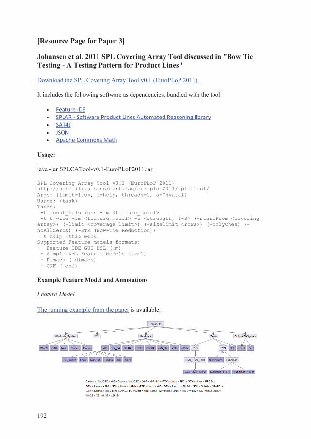
Feature IDE SPLAR - Software Product Lines Automated Reasoning library SAT4J JSON Apache Commons Math

SPL Covering Array Tool v0.1 (EuroPLoP 2011) http://heim.ifi.uio.no/martifag/europlop2011/splcatool/ Args: {limit=100%, t=help, threads=1, a=Chvatal} Usage: <task> Tasks: -t count_solutions -fm <feature_model> -t t_wise -fm <feature_model> -s <strength, 1-3> (-startFrom <covering array>) (-limit <coverage limit>) (-sizelimit <rows>) (-onlyOnes) (-noAllZeros) (-BTR (Bow-Tie Reduction)) -t help (this menu) Supported Feature models formats: - Feature IDE GUI DSL (.m) - Simple XML Feature Models (.xml) - Dimacs (.dimacs) - CNF (.cnf)

192

AL WindowingSystem AL Hardware AL OS

> java -jar SPLCATool-v0.1-EuroPLoP2011.jar -t t_wise -fm EclipseSPLRef.m -s 2 -BTR http://heim.ifi.uio.no/martifag/europlop2011/splcatool/ Args: {limit=100%, BTR=, fm=EclipseSPLRef.m, t=t_wise, s=2, threads=1, a=Chvatal} Loading GUI DSL: EclipseSPLRef.m Successfully loaded and converted the model: Features: 37 Constraints: 610 Generating 2-wise covering array with algorithm: Chvatal Running algorithm: Chvatal's algorithm adopted for Covering Array generation Covering 100% Uncovered pairs left: 2664 0/2664 ... Done. Size: 41, time: 1045 milliseconds BTR. Size: 20 Wrote result to EclipseSPLRef.m.ca2.csv Wrote result to EclipseSPLRef.m.ca2.csv.btr.csv

193

Contents

Tool Example Models

Tool

Feature IDE SPLAR - Software Product Lines Automated Reasoning library SAT4J JSON Apache Commons Math google-gson JavaBDD jgraph JUnit opencsv guidsl Jakarta

Generate a new Covering Array:

194

Calculate Coverage of an existing set of products:

Suggest improvements to a set of products:

195

Models

Feature model Weights Ordering

Feature model Products Weights Ordering

196

Applying the Technique for Testing of Eclipse-based Product Lines

"models", contains all input to the testing tools. "packages", contains all packages to be used to construct the software to be tested. "products", will store all built and tested products and their associated workspaces. "results", will store all generated results. "scripts", contains all scripts used for testing. "tools", contains all tools used for testing. "workspace", workspace for the Eclipse tool used to build the package repository.

1. 7-Zip Command Line Version (9.20) 2. Eclipse Platform (3.7.0) 3. UnxUtils (of 2007-03-01), Port of the most important GNU utilities to Windows 4. An implementation of Algorithm 3 from the paper (Contact us to get the source

code.)

1. Download the mirroring-script and place it in the scripts directory. Download and edit the environment set up script in which the path to the java.exe, cmd.exe and the root directory must be specified. Executing the mirroring script will construct mirrors for the Eclipse Indigo repositories in "%basedir%/packages/repos/". This will take a while, and might require rerunning the script several times to ensure that all packages were downloaded correctly. The size of these repositories during the experiments presented in the paper was 3.6 GiB.

2. Place a copy of the package containing the Eclipse Platform in "packages".

197

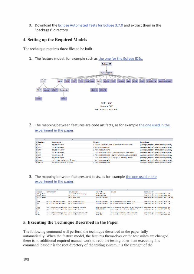
3. Download the Eclipse Automated Tests for Eclipse 3.7.0 and extract them in the "packages" directory.

1. The feature model, for example such as the one for the Eclipse IDEs.

2. The mapping between features are code artifacts, as for example the one used in the experiment in the paper.

3. The mapping between features and tests, as for example the one used in the experiment in the paper.

198

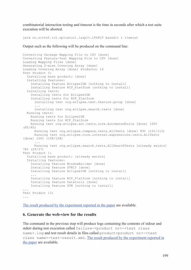
java no.sintef.ict.splcatool.lasplt.LTSPLT basedir t timeout

Converting Package Mapping File to CSV [done] Converting Feature-Test Mapping File to CSV [done] Loading Mapping Files [done] Generating 2-wise Covering Array [done] Loading Covering Array [done] Products: 14 Test Product 0: Installing base product: [done] Installing features: Installing feature EclipseIDE [nothing to install] Installing feature RCP_Platform [nothing to install] Installing tests: Installing tests for EclipseIDE Installing tests for RCP_Platform Installing test org.eclipse.test.feature.group [done] ... Installing test org.eclipse.search.tests [done] Running tests: Running tests for EclipseIDE Running tests for RCP_Platform Running test org.eclipse.ant.tests.core.AutomatedSuite [done] 100% (85/85) Running test org.eclipse.compare.tests.AllTests [done] 89% (101/113) Running test org.eclipse.core.internal.expressions.tests.AllTests [done] 100% (108/108) ... Running test org.eclipse.search.tests.AllSearchTests [already exists] 78% (29/37) Test Product 1: Installing base product: [already exists] Installing features: Installing feature WindowBuilder [done] Installing feature SVN15 [done] Installing feature EclipseIDE [nothing to install] ... Installing feature RCP_Platform [nothing to install] Installing feature Datatools [done] Installing feature SVN [nothing to install] ... Test Product 13: ...

failure-<product nr>-<test class name>.log product<product nr>-<test class name>-test-result.xml

199

java no.sintef.ict.splcatool.lasplt.GenerateWebView basedir

Applying the Technique for Testing of CVL-based Product Lines

A CVL model modelling the variability of the product line with bindings to the model artifacts. (Safety Module Case) Class path for test execution Feature-Test Mapping (Safety Module Case)

It also requires the following tools:

SPLCATool v0.3 (SPLC 2012) Java runtime 1.6 Eclipse 3.7.0 Eclipse Modeling Tools CVL Headless build (Plugin in CVL toolchain) JavaFrame Headless build (Plugin in CVL toolchain)

java -jar cvlsplt.jar

Extracting Feature Model from CVL Model: Done Generating 2-wise Covering Array: Done Injecting Covering Array into CVL model: Done Executing CVL: Generated %basepth%/model/product0.uml Generated %basepth%/model/product1.uml Generated %basepth%/model/product2.uml ... Generated %basepth%/model/product10.uml Generated %basepth%/model/product11.uml %basepth%/model/product0.uml Moving to %basepth%/JFWS/Product0/product.uml Running JavaFrame Generator: Exit code: 0 Building workspace: Exit code: 0 Building workspace: Exit code: 0 Run Tests: SafetyDrive.GeneralStartUp: [success] SafetyDrive.Level3StartUpTest: [success] Done %basepth%/model/product1.uml ...

200

Appendix B

Algorithms Based on WeightedSub-Product Line Models

In this appendix, we include details for algorithms related to weighted sub-product line models.

These were not included in Paper 4 because of space constraints. A free and open-source

implementation of them was released with SPLCATool v0.4 as resource material for the paper.

This appendix provides pseudo-code for the algorithms with some explanation.

B.1 Some New Terms

A weighted t-set is a 2-tuple (w, e) with w being the weight and e being a t-set. The set of all

weighted t-sets is called St.

A priority queue of weighted t-sets is called Pt. Pt is an object with twomethods: add((w, e)),

a method that adds a 2-tuple to the priority queue, and pop() : (w, e) a method that gets the 2-

tuple at the start of the queue and removes it from the queue.

A weighted sub-product line model, W , is a set of 2-tuples, a set of (w,C), where C is a

valid, partial configuration (or sub-product line model) of feature model FM and w is a weight

given to that sub-product line model.

B.2 Calculating Weights

Algorithm 4 takes a feature model, FM , a set of weighted sub-product line models, W , and a

strength t. It makes a priority queue with weighted t-sets.

Line 1 generates the set of all t-sets from the feature model. Line 2 creates an empty priority

queue. The loop at line 3 loops through each weighted sub-product line model. This will be

our basis when getting t-sets and their weights. If a t-set is not in W , it will not be included in

the sets to cover. This is essentially the same as getting a weight of 0. The loop at line 4 goes

through each t-set contained in the sub-product line model, detailed as Algorithm 5. The loop

at line 5 goes through each possible t-set. At line 6, we check whether the t-set is valid.

Lines 8–19 check whether the partial t-set gotten from W contains s. e contains s if each

assignment in e is in s, lines 9–12, or if the feature with a wild-card from e is in s, lines 13–18.

At line 14, x, the number of wild-cards, is counted.

201

Algorithm 4 Get Priority Queue of Valid, Weighted t-sets:

getWPriorityQueue(FM,W, t) : Pt

1: Tt ← FM.genT (t)2: Pt ← PriorityQueue(∅)3: for each pair (w,C) in W do4: for each t-set e in getTSets(C, t) do5: for each t-set s in Tt do6: if FM.isSatisfiable(s) then7: (isIn, x) ← (true, 0)8: for each assignment a in e do9: if a.a ∈ {true, false} then10: if a �∈ s then11: isIn ← false12: end if13: else14: x ← x+ 115: if a.f �∈ s.getFs() then16: isIn ← false17: end if18: end if19: end for20: if isIn then21: Pt.add((w/2

x, s))22: end if23: end if24: end for25: end for26: end for

If s is contained within e, then s is given the weight of the sub-product line divided by 2x,

lines 20–22; 2x is the number of t-sets contained in e.

Algorithm 5 Get t-sets in a Configuration: getTSets(C, t) : Tt

1: Tt ← ∅2: if t > 1 then3: Tt−1 ← getTSets(C, t− 1)4: for each t-set e in Tt−1 do5: for each assignment a ∈ C do6: Tt ← Tt ∪ ({a} ∪ e)7: end for8: end for9: else10: for each assignment a in C do11: Tt ← Tt ∪ {a}12: end for13: end if

A sub-algorithm of Algorithm 4 is Algorithm 5. The purpose of this algorithm is to generate

all t-sets, Tt, covered by a configuration, C, of strength t. The algorithm starts by initializing

a new, empty set, Tt, line 1. If the value of t is 1, all the assignments in C are added to Tt,

lines 10–12. If t is larger than 1, Tt−1 is generated, line 3. Then they are combined with every

possible assignment, lines 5–7. This recursive algorithm eventually generates all t-sets covered

by the configuration.

202

B.3 Generating a Weighted Covering Array

Ordinary covering arrays are generated by selecting the product that covers the most uncovered

t-sets first. A weighted covering array is generated by selecting the product that covers the most

weight first. Algorithm 6 is a modification of Algorithm 1 from Paper 2 for weighted covering

arrays.

Algorithm 6 takes a feature model, FM , a weighted sub-product line model W , a strength

t, and a percentage u. By selecting t-sets to cover from a priority queue of t-sets, prioritized

according to weight, the algorithm keeps generating products until it has covered a u-part, at

which point it stops.

Algorithm 6 Weighted Covering Array Generation: Adaption of Algorithm 1 from the SPLC

2012-paper

GenWeightedCoveringArray(FM,W, t, u) : Ct

1: Tt ← FM.genT (t)2: Pt ← getWPriorityQueue(FM,Tt,W, t)3: tw ← 04: for each t-set e in Pt do5: tw = tw + e.w6: end for7: (Ct, cw) ← (∅, 0)8: while true do9: (C,CO) ← (∅, ∅)10: for each t-set e in Pt do11: if FM.is_satisfiable(C ∪ e.e) then12: C ← C ∪ e.e13: CO ← CO ∪ {e.e}14: cw ← cw + e.w15: end if16: end for17: Pt ← Pt \ CO18: C ← FM.satisfy(C)19: Ct ← Ct ∪ {C}20: if cw/tw ≥ u then21: break

22: end if23: end while

Line 1–2 constructs the priority queue of valid t-sets, as described in Algorithm 4. Line

3–6 calculates the total weight of all weighted t-sets. It does this by iterating through the entire

priority queue and adding each weight into a total. At line 7, an empty covering array and an

integer of the weight covered is initialized. Obviously, having no products, the covered weight is

0. Next, the main loop spans from line 8–23. It keeps adding products until the weight covered

over the total weight is larger than or equal u. At this point the algorithm stops, lines 20-22.

At lines 10–16, t-sets are covered, beginning at the top of the priority queue and proceeding

downwards. When a t-set is covered, its weight is added to cw, the covered weight. At line 17,

the covered t-sets are removed from the priority queue. At lines 18–19 the new product is added

to the covering array, before deciding whether to stop at lines 20–22.

203

B.4 Generating Improvement Suggestions

Algorithm 7 describes how to generate suggestions for improvement of an existing covering

array. The algorithm takes a feature model, FM , a covering array, CA, a weighted sub-product

line model, W , a strength, t, and a number, n, of how many changes of a single product to

consider.

Algorithm 7 Generate Suggestions

genImpSug(FM,CA,W, t, n) : S

1: S ← ∅2: if n > 0 then3: orgcov = getWeightCoverage(FM,CA,W, t)4: S ← S ∪ genImpSug(FM,CA,W, t, n− 1)5: for each product C in CA do6: for each t-set e in getTSets(C, n) do7: for each assignment a in e do8: a.a ← ¬a.a9: end for10: if FM.isSatisfiable(C) then11: newcov = getWeightCoverage(FM,CA,W, t)12: if newcov > orgcov then13: S.add(newcov, e.copy())14: end if15: end if16: for each assignment a in e do17: a.a ← ¬a.a18: end for19: end for20: end for21: end if

Line 1 initializes a new set S that will contain the suggestions and their new coverage. If

the number of changes wanted is higher than 0, line 2, line 3 calculates the current weight

coverage of the covering array given. This algorithm is detailed as Algorithm 8. Then, at line

4, all changes of size one less than n is calculated. The algorithm then, at lines 5 and 6, iterates

through all products and all n-sets covered by them. (Note, that since we are searching for n

changes, we want the n-sets and not the t-sets.) All assignments in this n-set are reversed, lines

7–9, and, if the new configuration is valid (line 10), the new coverage is calculated (line 11).

If the new coverage is strictly larger than the original coverage, the suggestion is added to the

set of suggestions, S. The suggestion is copied into the set. The assignments are then restored,

lines 16–18.

Note that this algorithm is data-parallel. The set gotten at line 7 is huge, easily containing

millions of elements; the rest of the algorithm can be run in parallel on as many nodes, at most.

Algorithm 8 is called two places in Algorithm 7. The purpose of this algorithm is to calculate

the percentage of the total weight is covered, cov, by a covering array CA of feature model FM

of strength t, given the weights and the sub-product lines model W .

The algorithm proceeds by first getting the set of all weighted t-sets, line 1. Line 3–5

calculates the total weight. Lines 6–10 collects all t-sets covered by the covering array into a

set Tt. Note that since Tt is a set, duplicates do not occur. Then, the weight of all covered t-sets

are summed up, lines 11-17, and the percentage calculated and returned, line 18.

204

Algorithm 8 Generate Weight Coverage

getWeightCoverage(FM,CA,W, t) : cov

1: PT ← getWPriorityQueue(FM,FM.genT (t),W, t)2: (tw, cw, cov, Tt) ← (0, 0, 0, ∅)3: for each pair e in Pt do4: tw = tw + e.w5: end for6: for each product C in CA do7: for each t-set e in getTSets(C, t) do8: Tt ← Tt ∪ {e}9: end for10: end for11: for each t-set e in Tt do12: for each pair p in Pt do13: if e = p.e then14: cw = p.w15: end if16: end for17: end for18: cov ← cw/tw

205

Appendix C

Details for Comparisons

Table C.1, C.2, C.3, C.4 and C.5 shows the details of the average running time of ICPL, CASA,

MoSo-PoLiTe, IPOG algorithms and the basic algorithm, respectively.

Figure C.1, C.2 and C.3 show the time performance of the five algorithms with an estimated

line on a logarithmic scale. Notice how ICPL’s line is characteristically different from all the

other lines.

207

Table C.1: Performance of ICPL on Large Feature Models

*Average based on less than 100 measurements.

†Covering arrays for t-sets containing with only included features (1/8th of the t-sets), the memory usage

was limited to 128 GiB instead of 32 GiB, and the algorithm was allowed to run in 64 processors at 100%

activity instead of 6.

Feature Model\keys Features

Constraints

(CNF

clauses)

SAT

time

(ms)

1-

wise

size

1-

wise

time

(s)

2-

wise

size

2-

wise

time

(s)

3-

wise

size

3-

wise

time

(s)2.6.28.6-icse11.dimacs 6,888 187,193 125 25 89 *480 *33,702 – –

freebsd-icse11.dimacs 1,396 17,352 18 9 10 77 240 †78 †2,540

ecos-icse11.dimacs 1,244 2,768 12 6 2 63 185 †64 †973

Eshop-fm.xml 287 22 5 3 <1 21 5 108 457

Violet.m 101 90 1 2 <1 26 2 122 32

Berkeley.m 78 47 1 4 <1 23 1 99 10

arcade_game_pl_fm.xml 61 35 3 3 <1 18 1 64 5

Gg4.m 38 23 1 6 <1 20 1 61 2

...

Table C.2: Performance of CASA on Large Feature Models



Constraints

(CNF

clauses)

1-

wise

size

1-

wise

time

(s)

2-

wise

size

2-

wise

time

(s)

3-

wise

size

3-

wise

time

(s)2.6.28.6-icse11.dimacs 6,888 187,193 – – – – – –

freebsd-icse11.dimacs 1,396 17,352 – – – – – –

ecos-icse11.dimacs 1,244 2,768 *11 *51,705 – – – –

Eshop-fm.xml 287 22 5 1,274 *31 *10,040 – –

Violet.m 101 90 3 38 23 79 *93 *16,310

Berkeley.m 78 47 3 39 19 145 *77 *9,142

arcade_game_pl_fm.xml 61 35 3 22 13 32 46 1,999

Gg4.m 38 23 6 8 17 14 50 134

...

Table C.3: Performance of MoSo-PoLiTe on Large Feature Models



Constraints

(CNF

clauses)

1-

wise

size

1-

wise

time

(s)

2-

wise

size

2-

wise

time

(s)

3-

wise

size

3-

wise

time

(s)2.6.28.6-icse11.dimacs 6,888 187,193 – – – – – –


ecos-icse11.dimacs 1,244 2,768 – – – – – –

Eshop-fm.xml 287 22 – – – – – –

Violet.m 101 90 – – 90 <1 1,123 164

Berkeley.m 78 47 – – 42 <1 421 23

arcade_game_pl_fm.xml 61 35 – – 38 <1 271 4

Gg4.m 38 23 – – – – – –

...

208

Table C.4: Performance of IPOG on Large Feature Models



Constraints

(CNF

clauses)

1-

wise

size

1-

wise

time

(s)

2-

wise

size

2-

wise

time

(s)

3-

wise

size

3-

wise

time

(s)2.6.28.6-icse11.dimacs 6,888 187,193 – – – – – –


ecos-icse11.dimacs 1,244 2,768 – – – – – –

Eshop-fm.xml 287 22 – – – – – –

Violet.m 101 90 – – *27 *12,655 – –

Berkeley.m 78 47 – – *22 *3,087 – –

arcade_game_pl_fm.xml 61 35 – – *19 *5,858 *64 *45,632

Gg4.m 38 23 – – – – 77 2,442

...

Table C.5: Performance of Alg. 1 on Large Feature Models



Constraints

(CNF

clauses)

1-

wise

size

1-

wise

time

(s)

2-

wise

size

2-

wise

time

(s)

3-

wise

size

3-

wise

time

(s)2.6.28.6-icse11.dimacs 6,888 187,193 – – – – – –

freebsd-icse11.dimacs 1,396 17,352 7 165 – – – –

ecos-icse11.dimacs 1,244 2,768 6 13 – – – –

Eshop-fm.xml 287 22 4 1 22 44 – –

Violet.m 101 90 4 <1 28 4 124 233

Berkeley.m 78 47 3 <1 24 2 95 111

arcade_game_pl_fm.xml 61 35 4 <1 16 2 64 38

Gg4.m 38 23 6 <1 22 <1 63 7

...

209

100

1 000

10 000

100 000

1 000 000

10 100 1000

Alg. 1

CASA

ICPL

Figure C.1: Covering Array Sizes vs. Generation Time: 1-wise

10

100

1 000

10 000

100 000

1 000 000

10 000 000

10 100

Alg. 1

CASA

ICPL

IPOG

MoSo-Polite


10

100

1 000

10 000

100 000

1 000 000

10 000 000

10 100

Alg. 1

CASA

ICPL

IPOG

MoSo-Polite


210

Appendix D

Technical About the Tools

As a part of the research method, we implemented the algorithms that we made in order to

evaluate them in realistic settings. The Software Product Line Covering Array Tool (SPLCA-

Tool) implements various algorithms for working with feature models and covering arrays. It

includes various libraries from the community; thus, it integrates with formats and algorithms

in the research community and from industry.

D.1 Version History

Throughout the PhD project, the tool was updated to include our latest developed and published

results. Each release of the tools was named after the conference its implemented results were

published at. Here is the release history of the tools:

• SPLCATool v0.1 (EuroPLoP 2011) - Released 2011-06-14 as resource material for a

paper presented at EuroPLoP 2011 (Paper 3).

• SPLCATool v0.2 (MODELS 2011) - Released 2011-05-03 as resource material for paper

submitted to MODELS 2011 (Paper 1).

• SPLCATool v0.3 (SPLC 2012) - Released 2011-10-28 as resource material for a paper

published at SPLC 2012 (Paper 2).

• SPLCATool v0.4 (MODELS 2012) - Released 2012-04-03 as resource material for paper

submitted to MODELS 2012 (Paper 4).

• Automatic CIT Tool Collection (ICTSS 2012) - Released 2012-06-18 as resource ma-

terial for a paper submitted to ICTSS 2012 (Paper 5).

The tool provided us with a framework onto which new functionality could be added onto

and experimented with. It also was used to produce the empirical evaluations in the papers

published.

D.2 Architecture

The tool works with three kinds of artifacts given to it by the user along with some instructions

of what to do with them.

211

• Feature Models: In essence, any feature model that can be converted to a propositional

formula can be loaded by the tool. We have, however, only implemented some of the ma-

jor formats for feature modeling used in academia and industry. Whenever possible, the

libraries associated with a particular format have been used. When this was not possible,

custom loaders were developed. When the libraries contained bugs that stopped us, those

bugs were fixed.

• Covering Arrays: A covering array is a set (or an array) of configurations of a feature

model selected such that each t-sets, for some t, are covered (thereby the name coveringarray). Each configuration is a set of assignments such that all features are given an

assignment and such that the configuration is valid according to the feature model.

• Weighted Sub-Product Line Models: Similarly as covering arrays, sub-product line

models give assignments to features, but assignments can be left unassigned. The unas-

signed features thus maintain some variability, and the configurations of this partial fea-

ture model are a sub-set of all possible configurations. Therefore, they are called sub-

product line models. The models are called weighted because each sub-product line

model is given a positive integer as a weight.

The first set of functionalities provided by the tool is verification of the artifacts.

• Feature models have two basic requirements: (1) They must have valid syntax, and (2)

they must have at least one valid configuration. Both of these are checked by running the

is_satisfiable task.

• Covering arrays are valid and invalid relative to a feature model. Because a covering

array is a set of configurations of the feature model, they must, to be valid, be valid

configurations of the feature model. This is verified using the verify_solutions

task.

• Weighted sub-product line models are also valid or invalid relative to a feature model.

Because they are not configurations but sub-product lines, they have the same requirement

as feature models: They must give at least one valid configuration. This is checked by

running the verify_weighted_solutions task. In addition, the weights must be

positive integers.

The second set of functionalities is the various algorithms:

• Generating covering arrays: A covering array is produced from a feature model and a

strength t for the strength of the coverage. Various algorithms can be invoked for gen-

erating covering arrays. The algorithms all have different characteristics of (1) speed of

generation, (2) size of resulting covering array, (3) variance in results between invocations

and (4) supported additional features.

• Calculating the coverage of a set of products: Given a feature model and a set of

configuration and a strength t, the t-wise coverage of the products given the feature model

can be calculated. The coverage can be given either as a t-set coverage in percent of t-sets

212

covered by the configurations or as weight coverage in percent of the weight covered by

the configurations. To calculate weight coverage, a weighted sub-product line model is

also required.

• Generate a list of suggestions for improving the weight coverage of a set of products:Given a feature model, a set of products and a weighted sub-product line model, the set

of products might be improved by changing it slightly. Suggesting such small changes to

improve coverage is the role of this class of functionality.

D.2.1 Feature Model Formats

The following five formats are supported.

• GUI DSL Models (.m) This is a feature model format used by the Feature IDE tools

suite [155]. It is as a format by the AHEAD and GenVoca tools by Automated Software

Design Research Group at the University of Texas at Austin.

• Simple XML Feature Model (SXFM) (.xml) SXFM is a feature model format used to

store feature models for the Software Product Line Online Tools (SPLOT)1 developed

by the Generative Software Development Lab / Computer Systems Group, University Of

Waterloo, Canada, 2010.

• DIMACS CNF format (.dimacs) This is the format used by the SAT4J library. It has

become a standard format for Boolean formulas in CNF. It was initially proposed as a for-

mat for CNF formulas by the Center for Discrete Mathematics and Theoretical Computer

Science (DIMACS) [48].

• CVL 1.x (.xmi or .cvl) CVL is a variability-modeling format proposed in 2008 for adding

variability mechanisms to DSLs [69]. It is currently being considered as a standard for

variability-modeling by the OMG [71]. The version 2 of CVL is currently being devel-

oped. However, only the first version of the format is supported by SPLCATool. CVL

models can be created using the CVL Tool2.

Due to the richness of CVLmodels, a feature model must be extracted from it before it can

be loaded. Download the CVL Tool chain from the ICTSS 2012-paper resource page3,

unzip CVLUtils.jar and execute java -cp CVLUtils;CVLUtils/lib/*CVL2GDSL model.cvl to produce a Feature IDE GUI DSL file model.cvl.m. It

can be loaded with the normal loading procedure.

D.2.2 Configuration Set Formats

Covering Arrays are a set of configurations of a feature model. Thus, except for their special

property, they are no different from a set of configurations.

1http://gdansk.uwaterloo.ca:8088/SPLOT/sxfm.html, retrieved 2013-01-052http://www.omgwiki.org/variability/doku.php/doku.php?id=cvl_tool_from_

sintef3http://heim.ifi.uio.no/martifag/ictss2012/

213

• Comma Separated Values (CSV): Due to the use of the comma as a decimal mark in

Norway, Norwegian CSV files are semi-colon separated instead of comma-separated.

Configurations are stored in the following way, textually: The first entry in the file must

be "Feature\Product;". This means that the features will be listed in the rows, and the

products will be listed in the columns. This is the most practical arrangement for editing

and viewing. Following this entry, the names of the products are listed. This can be

as simple as 1, 2, 3 etc., written as "1;2;3;". On each line following the first line is a

feature name followed by either an "X" or a "-" when the feature is included or excluded,

respectively, for the product in that column. Editing these files in Excel or similar is of

course recommended.

• Excel Office Open XML (XSLX): These files are edited using Excel or similar. They

are loaded by the tool using the "Apache POI - Java API To Access Microsoft Format

Files"-library. There are some additional requirements when using this format in order

to delimit the product configurations and allow for additional comments and entries in

the file: (1) the entry following the lower-most feature must be "#end" and (2) the entry

following the last product name must also be "#end".

D.2.3 Weighted Sub-Product Line Formats

Weighted Sub-Product Line models are a set of configurations of a feature model with two ad-

ditional things added. Thus, except for their two additions, they are stored similarly to covering

arrays.

The two additions are: (1) Assignments can be left unassigned using a question mark. (2)

The feature on the first row is named "#Weight". On this row, the weight for each sub-product

line is given. It must be a positive, non-zero integer.

D.2.4 Versions

There are several versions and editions of the tool. Each version is named after the conference

at which the results it implements are published. For one version, there are several editions

because of licensing concerns.

• v0.1 (EuroPLoP 2011): This version introduced basic covering array generation for 1 ≤t ≤ 3 and implements the Bow-Tie reduction algorithm. The covering arrays were stored

in the CSV format.

• v0.2 (MODELS 2011): This version introduced 4-wise covering array generation, SAT-

timing, t-wise coverage calculation and the verification of the solutions in a covering

array.

• v0.3 (SPLC 2012): This version of the tool introduced an implementation of the ICPL

algorithm for 1 ≤ t ≤ 3. In addition, it implements support for running the IPOG, CASA

and MoSo-PoLiTe algorithms; however, these are only available in the Full edition of the

tool. It cannot be freely distributed because of licensing concerns. However, an edition

with the adaptors only (The Adaptors Only Edition) is available into which the three tools

214

can be added to produce the full edition. The IPOG algorithms supports covering array

generation for 1 ≤ t ≤ 6, CASA for 1 ≤ t ≤ 6 and MoSo-PoLiTe for 2 ≤ t ≤ 3.

• v0.4 (MODELS 2012): This version of the tool introduced implementations of algo-

rithms related to weighted sub-product line models. In addition, a GUI was introduced to

make working with the models easier; the output is still written to the command line how-

ever. The command-line interface is still available by extracting SPLCATool-v0.4-

MODELS2012.jar and calling java -cp SPLCATool-v0.4-MODELS2012;

SPLCATool-v0.4-MODELS2012 no.sintef.ict.splcatool.SPLCATool.

The tool introduced (1) the generation of covering arrays prioritized using the weighted

models, (2) the verification of weighted sub-product line models, and (3) the improvement

of existing covering arrays using the weighted sub-product line models. This version also

introduced the loading of covering arrays in the XLSX format.

• Automatic CIT Tool Collection (ICTSS 2012): The Automatic CIT Tool introduced

scripts, formats and the implementation of the algorithms for automatic CIT both for

Eclipse- and CVL-based product lines. It also introduced a support for extracting GUI

DSL models from CVL-models, thereby enabling the generation of covering arrays from

feature models within CVL models.

D.2.5 Overview of Algorithms and Object Structures

Inside the tool, the different formats are imported and converted into other formats in order to

be applicable for various algorithms. Figure D.1 shows an overview of the transformations,

what formats are fed to the different algorithms and what these algorithms produce. The figure

is of no particular modeling notation. First of all, feature models can be given to the tool in

the four different formats. They are converted in one direction. After being converted, some

of the formats have exporting to file implemented. Covering arrays are read in from CSV and

XLSX files. Weighed sub-product line models can also be read in from CSV and XLSX files.

The rectangular boxes symbolize internal object-structures; the arrows symbolize algorithms

that generate some other data.

The various algorithms available are further described in the basic user manual, Section D.3.

D.3 User Manual

This basic user manual explains how to use the tool using the Eclipse case study as a running

example. The four files for the Eclipse case study are available on the resource page of the

MODELS 2012-paper4.

• Products — eclipse-red.m.actual.csv

• Feature model — Eclipse.m

• Weights — eclipse-red.m.actual-weighted.csv

• Ordering — eclipse.m.order.csv

4http://heim.ifi.uio.no/martifag/models2012/

215

Figure D.1: Transformations in the Tool

The products are the configurations of the 12 products that were available for download on

the Eclipse v3.7.0 (Indigo) web site. They are valid configurations of the feature model that

captures the relations between the different features of the Eclipse product line. The weights-

file contains the current market-situation—it was captured by adding the number of downloads

to each product offered. This is a basic approximation because we have no clue as to how the

users proceeded to configure their products. The ordering files contain the order the features

should be listed in the generated files. This is necessary because there is no intrinsic order to

the features in the other files.

Throughout the manual, the command-line will be used. Only the arguments of the command-

line invocations will be shown.

D.3.1 Analysis

First, let us check the validity of the files and find out some basic information about them. Let

us first check the feature model. The sat_time task (v0.4) will attempt to load the feature

model; if successful, it will print some basic information about it and try to find a single valid

configuration. It will then report whether one exists and how long time it took to find it, its

satisfiability-time. Execute -t sat_time -fm Eclipse.m (v0.4) to run the task. This

information is returned:

• Valid feature model?: yes

• Number of Features: 26

• Number of CNF-clauses of the composed constraint: 6

• Satisfiable?: yes

• Satisfying time: 0.446 ms

216

Thus, we know several important things: The feature model is valid and it has a very fast

satisfiability time. This means it is fully usable for all other tasks.

Let us try to find one additional piece of information, the number of valid configurations.

Run -t count_solutions -fm Eclipse.m (v0.4). This task does not scale very well;

up to about 200 features should work on modern hardware.

• Number of possible configurations: 1,900,544.

This is an enormous number; log2(1, 900, 544) ≈ 21, which is relatively close to 26, the number

of features of the feature model. If each feature is a yes-or-no choice, and each choice was

independent, then the number of configurations would be 2f , where f is the number of features.

Features normally are not independent, but 2f still gives us an idea of the magnitude of the

number of configurations.

Let us now analyze the products. Run -t verify_solutions -fm Eclipse.m

-check eclipse-red.m.actual.csv (v0.4). This task will check whether the config-

urations are valid according to the feature model. It tells us that it is. Had it been invalid, the

tool would output the CNF-clauses that were not satisfied. This gives us a good guide as to

where to look for the problem.

Let us analyze the weighted sub-product line model. Run -t verify_weighted_

solutions -fm Eclipse.m -check eclipse-red.m.actual-weighted.csv

(v0.4). This task will check whether the partial configurations are valid. It tells us that it is.

Again, had it been invalid, it would tell us which CNF-clauses were not satisfied.

• Configurations valid?: yes

• Weighted sub-product line models valid?: yes

Finally, let us find the t-set and weight coverage of the products. Run -t calc_cov -fm

Eclipse.m -s <t> -ca eclipse-red.m.actual.csv (v0.4) to find the t-set cov-

erage and -t calc_cov_weighted -fm Eclipse.m -s <t> -ca eclipse-red

.m.actual.csv -weights eclipse-red.m.actual-weighted.csv (v0.4) to find

the weight coverage, both for 1 ≤ t ≤ 3. That gives the following coverages:

• 1-set coverage: 49/50 ≈ 98.0%

• 2-set coverage: 929/1, 188 ≈ 78.2%

• 3-set coverage: 10, 034/17, 877 ≈ 56.1%

• 1-wise weight coverage: 52, 949, 676/52, 949, 676 = 100%

• 2-wise weight coverage: 661, 870, 950/661, 870, 950 = 100%

• 3-wise weight coverage: 2, 623, 612, 957/2, 623, 612, 957 = 100%

It is not a surprise that the weight coverage is 100%. It is because the weighted sub-product

line model contains only the products that are offered. It would be better to have actual informa-

tion about the market, but such information is unavailable, unfortunately. The TOMRA models

are unavailable due to sensitivity concerns.

The denominators of the t-set coverage are 50, 1,188 and 17,877. These are the number of

valid 1, 2 and 3-sets, respectively. When all are covered, we have a complete t-wise covering

array.

217

The denominators of the weight coverage are 52,949,676, 661,870,950 and 2,623,612,957.

These are the total weight for all valid 1, 2 and 3-sets, respectively. When all the weight is

covered, the weighted covering array has a coverage of 100%.

D.3.2 Generating Covering Arrays

Now that we have analyzed all our models and checked their validity, let us generate some new

things and then verify them.

Generate a t-wise covering array for 1 ≤ t ≤ 3 using ICPL by running -t t_wise -a

ICPL -fm Eclipse.m -s <t> (v0.3 (ICPL Edition)). This results in the following files

containing the covering arrays.

• Eclipse.m.ca1.csv, products: 2, generation time: 26 ms



Calculating the coverage of each using the same method as discussed above yields 100%

1, 2 and 3-wise coverage, respectively, as expected. Notice that the 12 products offered by

Eclipse have a 2-wise coverage of 78.2% while 12 products are also needed to yield 100%

2-wise coverage!

It is also possible to calculate covering arrays using other algorithms. Because of licensing

issues, we cannot distribute the full edition of the tool. However, once these tools have been

acquired, the following commands can be used to calculate covering arrays using other algo-

rithms: -t t_wise -a <a> -fm Eclipse.m -s <t> (v0.3 (Full Edition)) where a

is IPOG, CASA or MoSoPoLiTe. These three support 1 ≤ t ≤ 6, 1 ≤ t ≤ 6 and 2 ≤ t ≤ 3,

respectively.

If 12 products, a complete 2-wise covering array, are too costly for testing in your context,

and you would like to get a smaller set that is still related to the market situation, you can use

weighted covering array generation. Let us say we decide to cover 95% of the weight. Run -t

t_wise_weighted -a ChvatalWeighted -fm Eclipse.m -s <t> -weights

eclipse-red.m.actual-weighted.csv -limit 95% (v0.4) for 2 ≤ t ≤ 3 to pro-

duce the following results:



Calculating the weighted coverage using the methods discussed above yields 97.05% and

95.08% 2 and 3-wise weight coverage, respectively. Both are, as required, equal to or above

95%.

D.3.3 Extending Towards a Covering Array

A realistic situation when doing product line testing is that certain popular and important prod-

ucts must be tested. For example, for Eclipse, 3 products account for 88% of the downloaded

products. Instead of just adding these 3 products to the already complete covering arrays, we

could start from them to probably make them be a part of the covering array.

218

Extract the "Java", "Java EE" and "Classic" products into a file called eclipse-red.m.

important.csv. To include them in a covering array run -t t_wise -a ICPL -fm

Eclipse.m -s <t> -startFrom eclipse-red.m.important.csv (v0.3 (ICPL

Edition)). The extended versions are:

• Eclipse.m.ca1.csv, products: 5, time: 27 milliseconds



For 1-wise testing, this does not reduce the effort because there were three important prod-

ucts, but only two were required to achieve 1-wise coverage. For 2-wise testing, the new cover-

ing array has 13, only one more than a fresh 2-wise covering array. For 3-wise testing, the new

covering array has 40 products, also only one more than the 39 required when building a fresh

covering array.

We can also extend covering arrays based on weight. If we start with the three important

products again, let us see what is needed to extend with one more product. We could also extend

based on percentages, but this opportunity is used to demo the size limits.

First of all, the weight coverages of the 3 important products are 98.68%, 97.05% and

95.08%, respectively. Run the following command to extend the set of products with a max-

imum of two new product based on maximizing the weight coverage starting from three im-

portant products for 1 ≤ t ≤ 3: -t t_wise_weighted -a ChvatalWeighted -fm

Eclipse.m -s <t> -weights eclipse-red.m.actual-weighted.csv

-startfrom eclipse-red.m.important.csv -sizelimit 5 (v0.4). The new

set of products of sizes 4, 5 and 5 has weight coverages of 100%, 99.5% and 98.5%, respec-

tively.

D.3.4 Improving a Partial Covering Array

In settings where a complete test system has been set up; for example, if the products of a

hardware product line has been physically set up, it is not good to have drastic changes to the

product configurations.

The tool supports suggesting small changes to an existing set of products to improve its

weight coverage.

An especially important usage of this is in the following situation: A product line gets a new

feature added to it. The company already has a test lab of, say, 12 products set up. The question

now is: To which product is it best to add this feature to maximize the coverage with respect to

the market situation (the weight coverage)?

First add a new feature to Eclipse.m named X as an optional feature of RCP_Platform,

then add a new row to the set of product offered by Eclipse with X set to all excluded (’-’),

then finally, add a new row to the weighted sub-product line model with all unassigned (’?’).

This row of unassigneds tells the tool, in effect, that we do not know who will be using the

new feature, so we had better ensure that it is exercised during testing and that it is tested out

together with the other features.

To have the tool figure this out automatically, run -t improve_weighted -fm

Eclipse.m -s 2 -ca eclipse-red.m.actual.csv -weights

219

eclipse-red.m.actual-weighted.csv -search 1 > list.txt (v0.4). Here,

we assume that the offered products are also the products that the Eclipse Projects tests, a real-

istic assumption. We want to maximize our 2-wise interaction coverage, which means that we

want our new feature to be exercised against any other feature. Finally, we want to maximize

the weight coverage to ensure market relevance. Because we only want to activate a single fea-

ture, we only search for single changes, -search 1. Running the task results in the following

results:

• Original weight coverage: 96.3%

• Suggested change: Set feature X to included for the product named "1" (the second prod-

uct).

• New weight coverage: 99.3%.

• Time taken: about 2 seconds.

D.3.5 Automatic CIT: Eclipse-Based Product Lines

This part of the manual explains how to apply Automatic CIT to Eclipse-based product lines.

The first thing that is needed is to set up the directory structure where all files will go. First,

decide on a root directory in which all files related to the testing will be stored. In this directory,

create these directories:

• models— contains all input to the testing tools.

• packages— contains all packages to be used to construct the software to be tested.

• products— will store all built and tested products and their associated workspaces.

• results— will store all generated results.

• scripts— contains all scripts used for testing.

• tools— contains all tools used for testing.

• workspace— workspace for the Eclipse tool used to build the package repository.

The next step is to acquire the required tools. Links are available from the ICTSS 2012-

paper resource page5. Note that all downloads mentioned in this part of the manual is found on

that resource page. Download and extract the following free tools in the "tools" directory.

• 7-Zip Command Line Version (9.20)

• Eclipse Platform (3.7.0)

• UnxUtils (of 2007-03-01), ports of the most important GNU utilities to Windows

• An implementation of Algorithm 3 from the paper

The next step is to build the package repository. Download the mirroring-script, and place

it in the scripts directory. Download and edit the environment set up script in which the path to

the java.exe, cmd.exe and the root directory must be specified. Executing the mirroring script

will construct mirrors for the Eclipse Indigo repositories in "%basedir%/packages/repos/". This

will take a while and might require rerunning the script several times to ensure that all packages

5Appendix A or http://heim.ifi.uio.no/martifag/ictss2012/

220

were downloaded correctly. The size of these repositories during the experiments presented in

the paper was 3.6 GiB.

Place a copy of the package containing the Eclipse Platform in "packages". Download the

Eclipse Automated Tests for Eclipse 3.7.0. Inside it there is a zip-file called eclipse

-testing/eclipse-junit-tests-I20110613-1736.zip. Extract it in the "pack-

ages" directory.

The next step is setting up the required models. The technique requires three files to be

built: (1) The feature model, for example such as the one for the Eclipse IDEs. (2) The mapping

between features and code artifacts, as for example the one used in the experiment in the paper.

(3) The mapping between features and tests, as for example the one used in the experiment in

the paper. Examples of these files for the Eclipse 3.7.0 system are available on the resource

page.

The next step is execution. The following command will execute Automatic CIT: java

no.sintef.ict.splcatool.lasplt.LTSPLT <basedir> <t> <timeout>.

basedir is the root directory of the testing system, t is the strength of the combinatorial

interaction testing and timeout is the time in seconds after which a test suite execution will be

aborted.

When the feature model, the features themselves or the test suites are changed, there is

no additionally required manual work to redo the testing other than re-executing the above

command.

Output such as the following will be produced on the command line:

Converting Package Mapping File to CSV [done]

Converting Feature-Test Mapping File to CSV [done]

Loading Mapping Files [done]

Generating 2-wise Covering Array [done]

Loading Covering Array [done] Products: 14

Test Product 0:

Installing base product: [done]

Installing features:

Installing feature EclipseIDE [nothing to install]

Installing feature RCP_Platform [nothing to install]

Installing tests:

Installing tests for EclipseIDE

Installing tests for RCP_Platform

Installing test org.eclipse.test.feature.group [done]

...

Installing test org.eclipse.search.tests [done]

Running tests:

Running tests for EclipseIDE

Running tests for RCP_Platform

Running test org.eclipse.ant.tests.core.AutomatedSuite [done] 100%

(85/85)

Running test org.eclipse.compare.tests.AllTests [done] 89% (101/113)

Running test org.eclipse.core.internal.expressions.tests.AllTests [

done] 100% (108/108)

...

Running test org.eclipse.search.tests.AllSearchTests [already exists]

78% (29/37)

221

Test Product 1:

Installing base product: [already exists]

Installing features:

Installing feature WindowBuilder [done]

Installing feature SVN15 [done]

Installing feature EclipseIDE [nothing to install]

...

Installing feature RCP_Platform [nothing to install]

Installing feature Datatools [done]

Installing feature SVN [nothing to install]

...

Test Product 13:

...

As a final stage, it is possible to generate a web-view for the results. This is good for using

Automatic CIT in conjunction with continuous integration system such as Hudson6 or Jenkins7.

The command in the previous step will produce logs containing the contents of stdout andstderr during test execution called failure-<product nr>-<test class name>.log

and test result details in files called product<product nr>-<test class name>

-test-result.xml. The results produced by the experiment reported in the paper are

available on the resource page of Paper 5.

These results can be compiled into a report by executing the following command: java

no.sintef.ict.splcatool.lasplt.GenerateWebView <basedir> This will

produce an HTML-document. An example for the Eclipse IDE experiment is found on the

resource page of Paper 5.

D.3.6 Automatic CIT: CVL Based Product Lines

Automatic CIT can be applied to CVL-based product lines in a similar way to Eclipse-based

product lines. The set up required is found in CVLLASPLTInput.java a template found

in CVL tool chain available from the resource page website. The guidelines for Eclipse-based

product lines can be used to understand how to run Automatic CIT for CVL-based product

lines.

6http://hudson-ci.org/7http://jenkins-ci.org/

222

Appendix E

Details on the Eclipse Case Study

The Eclipse IDEs are used as a case study in the EuroPLoP 2011, MODELS 2012 and ICTSS

2012 papers. All experiments used Version 3.7.0 (Indigo) of Eclipse; it was released in the

summer of 2011.

E.1 Technical About Eclipse v3.7.0 (Indigo)

The architecture and design of Eclipse is documented in Rivieres and Beaton 2006 [132]. The

development of Eclipse is open, and most development artifacts, choices made and design de-

cisions are recorded online.

Twelve products are offered online by the Eclipse Project. The configurations of these

products are shown online as a matrix, shown in Figure E.1.

These products are available for 15 combinations of operating system, windowing systems

and hardware architectures. The list of 15 builds available from the Eclipse project is shown in

Figure E.2.

Further, the Eclipse Project specifies which versions are supported. These are shown in

Figure E.31. According to their documentation, "Eclipse 3.7 is tested and validated on the

following reference platforms".

Eclipse IDE products are built from OSGi bundles [63]. These software assets are identified

by a pair (id : ID, version : V ), where id is an ID string unique for that bundle conforming to

a grammar for IDs which is the same as the naming conventions for Java packages, and version

is a versioning string valid according to one of several version grammars. The version grammar

used by the Eclipse plug-in system is i(.i(.i(.s)?)?)? where i are positive integers including 0

and s is a string. The integers are respectively called ’major’, ’minor’, then either ’micro’ or

’service’, and, finally, the ’s’ is called ’qualifier’.

Bundles are stored in Java archives named id_version.jar. They are published online2.

The basic Eclipse platform is distributed as a zip-package. This package can be extracted

into a new folder and is then ready to use. It contains the capabilities to allow each feature and

test suite to be installed automatically using the following command:

1http://web.archive.org/web/20110608032901/http://www.eclipse.org/projects/project-plan.php?projectid=eclipse

2http://download.eclipse.org/releases/indigo/

223

Figure E.1: Product Configuration of the Twelve Eclipse IDE Products Offered by the Eclipse

Project

Figure E.2: Builds Available from the Eclipse Projects

224

Figure E.3: Supported Versions of Environment Artifacts

<eclipse executable> -application org.eclipse.equinox.p2.director -

repository <repository1,...> -installIU <id>/<version>

E.2 Contributed Artifacts

As for all of the other case studies, Eclipse does not employ an explicit product line methodol-

ogy. As is quite clear, however, their approach is at least very close. It was quite easy to build a

feature model by browsing through their bundles.

From any bundle b∈B it is possible to extract a set bd with the dependencies of bundle b.

The dependencies is a set of pairs (id : ID, vr : V R), where id is an ID and vr is a string

specifying a range of versions according to grammars of ranges of versions. Figure E.4 shows

the complete feature diagram of the Eclipse IDEs. The products shown in E.2 are of course

valid (partial) configurations of this feature model.

E.3 Details on Automatic CIT of Eclipse

This section details the large-scale application of the Automatic CIT technique to the entire

Eclipse IDE Indigo (v3.7.0) product line supported and maintained by the Eclipse Project.

For the experiment in Paper 5, the part of the Eclipse IDE product line shown in Figure E.5

was selected for testing; three additional features were included. The products offered by

225

EclipseIDE

RCP_Platform

JDT

PDE

Scout

Maven

EMF

GMF

Datatools

BIRT GEF

CDT

CVSWebTools

SVNMylyn

PTPJubula

RAP

EGit

RSEEclipseLink

Window

BuilderPlatform

Window

ingSystem

Win32

GTK

Motif

CarbonCocoa

OS

OS_W

in32Linux

MacO

SXSolaris

AIX

hpux

Hardw

are

x86x86_64

SPARC

PPCPPC64

ia64_32s390

s390x

GM

F ⇒ G

EF

Maven ⇒

EMF

BIRT ⇒

GEF ∧ JD

T ∧ PDE

Carbon ∧ M

acOSX ∧ x86 ∨ C

ocoa ∧ MacO

SX ∧ (x86 ∨ x86_64) ∨ G

TK ∧ Linux ∧ PPC ∨ G

TK ∧ Linux ∧ PPC64 ∨

GTK ∧ Linux ∧ s390 ∨ G

TK ∧ Linux ∧ s390x ∨ G

TK ∧ Linux ∧ x86 ∨ GTK ∧ Linux ∧ x86_64 ∨

GTK ∧ Solaris ∧ SPAR

C ∨ G

TK ∧ Solaris ∧ x86 ∨ M

otif ∧ AIX ∧ PPC ∨ M

otif ∧ hpux ∧ ia64_32 ∨ M

otif ∧ Linux ∧ x86 ∨ Win32 ∧ O

S_Win32 ∧ x86 ∨

Win32 ∧ O

S_Win32 ∧ x86_64

Figure

E.4:Featu

reDiag

ramofthepart

ofEclip

seID

EIndigo(v3.7.0)su

pported

bytheEclip

seProject

226

EclipseIDE

RCP_Platform

JDT

PDE

Scout

Maven

EMF

GMF Datatools

BIRT

GEF CDT CVS WebTools SVN

SVN15 SVN16

Mylyn PTP Jubula RAP EGit RSE EclipseLink WindowBuilder

Maven ⇒ EMFBIRT ⇒ GEF ∧ JDT ∧ PDE

GMF ⇒ GEF

Figure E.5: Feature Model for the Eclipse IDE Product Line

Table E.1: Eclipse IDE Products, Instances of the Feature Model in Figure E.5

(a) Official Eclipse IDE products

Feature\Product 1 2 3 4 5 6 7 8 9 101112

EclipseIDE XXXXXXXXXX X X

RCP_Platform XXXXXXXXXX X X

CVS XXXXXXXXXX X X

EGit - - XXXX - - - - - -

EMF XX - - - XX - - - - -

GEF XX - - - XX - - - - -

JDT XX - - XXX - X - - X

Mylyn XXXXXXXXXX X -

WebTools - X - - - - X - - - X -

RSE - XXX - - XX - - - -

EclipseLink - X - - - - X - - X - -

PDE - X - - XXX - X - - X

Datatools - X - - - - X - - - - -

CDT - - XX - - - X - - - -

BIRT - - - - - - X - - - - -

GMF - - - - - X - - - - - -

PTP - - - - - - - X - - - -

Scout - - - - - - - - X - - -

Jubula - - - - - - - - - X - -

RAP - - - - X - - - - - - -

WindowBuilder X - - - - - - - - - - -

Maven X - - - - - - - - - - -

SVN - - - - - - - - - - - -

SVN15 - - - - - - - - - - - -

SVN16 - - - - - - - - - - - -

(b) Pair-wise Covering Array

Feature\Product 1 2 3 4 5 6 7 8 9 10111213

EclipseIDE XXXXXXXXXX X X X

RCP_Platform XXXXXXXXXX X X X

CVS - X - X - X - - X - - - -

EGit - X - - XXX - - X - - -

EMF - XXXX - - XXX X X -

GEF - - XXX - XXX - - X -

JDT - XXXX - X - XX - X -

Mylyn - X - X - - XX - - - - -

WebTools - - XXX - X - - X X - -

RSE - XX - XX - - - - - - -

EclipseLink - XX - - X - XX - - - -

PDE - X - XX - X - X - - X -

Datatools - XXXX - - - X - X X -

CDT - - XX - X - XX - - - -

BIRT - - - XX - - - X - - X -

GMF - - XXX - - XX - - - -

PTP - - X - XX - XX - - - -

Scout - X - X - - X - X - - - -

Jubula - - XX - X - X - X - - -

RAP - XX - - XX - X - - - -

WindowBuilder - X - X - X - X - - - - -

Maven - XX - - - - - X X - - -

SVN - X - - XXXXX - X - X

SVN15 - X - - X - - X - - - - X

SVN16 - - - - - XX - X - X - -

Eclipse and a 2-wise covering array are shown in Table E.1.

The different features of the Eclipse IDE are developed by different teams, and each team

has test suites for their feature. Thus, the mapping between the features and the test suites are

easily available.

The Eclipse Platform comes with built-in facilities for installing new features. We can start

from a fresh copy of the bare Eclipse Platform, which is an Eclipse IDE with just the core

features. When all features of a product have been installed, we can run the test suite associated

with each feature (or a combination of features).

E.3.1 Feature Models and Covering Arrays

There are many tools for doing feature modeling and generating covering arrays. For our im-

plementation we use Feature IDE to model the feature model as shown in Figure E.5, and our

SPL Covering Array Tool suite introduced in Paper 4 which is freely available on the paper’s

227

resource website. The covering array generated from the running example using this tool is

presented in Table E.1b.

E.3.2 Implementation with the Eclipse Platform’s Plug-in System

Algorithm 9 shows the algorithm of our testing technique for the Eclipse Platform plug-in sys-

tem3. The algorithm assumes that the following is given: a feature model, FM , and a coverage

strength, t.

In the experiment in the previous section, we provided the feature model in Figure E.5. The

algorithm loops through each configuration in the covering array. In the experiment, it was the

one given in Table E.1b. For each configuration, a version of Eclipse is constructed: The basic

Eclipse platform is distributed as a package. This package can be extracted into a new folder

and is then ready to be used. It contains the capabilities to allow each feature and test suite to

be installed automatically using the following command:


repository <repository1,...> -installIU <id>/<version>

Similar commands allow tests to be executed.

A mapping file provides the links between the features and the test suites. This allows

Algorithm 9 to select the relevant tests for each product and to run them against the build of the

Eclipse IDE. The results are put into their respective entry in the result table. (An example is

shown later in Table E.4b.)

3The source code for this implementation including its dependencies is available through the paper’s resource

website, along with the details of the test execution and detailed instructions and scripts to reproduce the experi-

ment.

Algorithm 9 Pseudo Code of Eclipse-based version of Automatic CIT

1: CA ←FM.GenerateCoveringArray(t)2: for each configuration c in CA do3: p ← GetBasicEclipseP latform()4: for each feature f in c do5: p.installFeature(f)6: end for7: for each feature f in c do8: tests ← f.getAssociatedTests()9: for each test test in tests do

10: p.installT est(test)11: result ← p.runTest(test)12: table.put(result, c, f)13: end for14: end for15: end for

228

Table E.2: Part of the Relation between Feature Names and Eclipse Bundle ID, Version and

Repository

Feature Bundle Version Repository

CVS org.eclipse.cvs 1.3.100... RepoA

EGit org.eclipse.egit 1.0.0... RepoA

EMF org.eclipse.emf 2.7.0... RepoA

GEF org.eclipse.gef 3.7.0... RepoA

JDT org.eclipse.jdt 3.7.0... RepoA

PDE org.eclipse.pde 3.7.0... RepoA

CDT org.eclipse.cdt 8.0.0... RepoA

BIRT org.eclipse.birt 3.7.0... RepoA

GMF org.eclipse.gmf 1.5.0... RepoA

SVN16 org.polarion.eclipse.team.svn.connector.svnkit16 2.2.2... RepoA, RepoB

SVN15 org.polarion.eclipse.team.svn.connector.svnkit15 2.2.2... RepoA, RepoB

... ... ... ...

E.3.3 Bindings Between Feature Names and System Artifacts

We require bindings from the feature names to the system artifacts. Feature names are found in

the feature model and in the covering array. For Eclipse-based product lines, system artifacts

are identified as with a bundle ID and a version. We also need to know where we can find

the system artifacts. Thus, we also need the URL(s) of the artifact and its dependencies. This

information can be easily entered in a spreadsheet and exported as a Comma Separated Values

(CSV) file. The testing system takes this file as input along with the feature model.

For the running example, an excerpt from such a relation is shown in Table E.24. Note that

the table has been reduced for presentation in this document. The bundles all really end with

.feature.group, some versions end with a hash and the repositories have been replaced

with a symbolic name. RepoA is the Eclipse update site, and RepoB is the Polarion update site

for subversive.

E.3.4 Automatic Building

We are now in a position to automatically build any Eclipse product. Start with a bundle of the

Eclipse platform, and, for each product, run the following command for each feature:


repository <repository1,...> -installIU <bundle>/<version>

Since the feature name is bound to the bundle ID, bundle version and repositories, we can

simply enter that information to the above boilerplate. After this is done all the products are set

up.

For the running example, setting up the 13 products of the covering array took about 1

hour, and it resulted in about 2.9 GB of Eclipse IDE products. The repositories were locally

mirrored5. For regular usage of this technique, it would be impractical to download the same

files again and again. Therefore, executing the technique with the local mirror is realistic.

4The full tables from the experiment as well as the implementation is available online at http://heim.ifi.uio.no/martifag/ictss2012/. On this website, everything to reproduce out experiment is available

for free.5The local cashes of the update sites takes 3.09 GB and took about 6–7 hours to download at SINTEF.

229

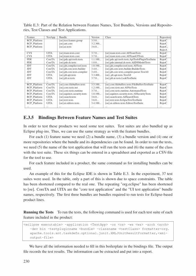
Table E.3: Part of the Relation between Feature Names, Test Bundles, Versions and Reposito-

ries, Test Classes and Test Applications.

Feature TestApp Bundle Version Class Repository

RCP_Platform [oe].test.feature.group 3.5.0... RepoC

RCP_Platform [oe].ant.core 3.2.300... RepoC

RCP_Platform [oe].ui.tests 3.6.0... RepoC,

RepoA

CVS UITA [oe].team.tests.core 3.7.0... [oe].team.tests.core.AllTeamTests RepoC

CVS UITA [oe].team.tests.core 3.7.0... [oe].team.tests.core.AllTeamUITests RepoC

PDE CoreTA [oe].pde.api.tools.tests 1.1.100... [oe].pde.api.tools.tests.ApiToolsPluginTestSuite RepoC

PDE CoreTA [oe].pde.ds.tests 1.0.0... [oe].pde.internal.ds.tests.AllDSModelTests RepoC

JDT CoreTA [oe].jdt.compiler.tool.tests 1.0.100... [oe].jdt.compiler.tool.tests.AllTests RepoC

JDT CoreTA [oe].jdt.core.tests.builder 3.4.0... [oe].jdt.core.tests.builder.BuilderTests RepoC

JDT CoreTA [oe].jdt.core.tests.compiler 3.4.0... [oe].jdt.core.tests.compiler.parser.TestAll RepoC

JDT UITA [oe].jdt.apt.tests 3.3.400... [oe]..jdt.apt.tests.TestAll RepoC

JDT UITA [oe].jdt.ui.tests 3.7.0... [oe].jdt.ui.tests.LeakTestSuite RepoC

... ... ... ... ... ...

RCP_Platform CoreTA [oe].core.filebuffers.tests 3.5.100... [oe].core.filebuffers.tests.FileBuffersTestSuite RepoC

RCP_Platform CoreTA [oe].core.tests.net 1.2.100... [oe].core.tests.net.AllNetTests RepoC

RCP_Platform CoreTA [oe].core.tests.runtime 3.7.0... [oe].core.tests.runtime.AutomatedTests RepoC

RCP_Platform CoreTA [oe].equinox.security.tests 1.0.100... [oe].equinox.security.tests.AllSecurityTests RepoC

RCP_Platform UITA [oe].search.tests 3.6.0... [oe].search.tests.AllSearchTests RepoC

RCP_Platform UITA [oe].text.tests 3.6.0... [oe].text.tests.EclipseTextTestSuite RepoC

RCP_Platform UITA [oe].ui.editors.tests 3.4.100... [oe].ui.editors.tests.EditorsTestSuite RepoC

... ... ... ... ... ...

E.3.5 Bindings Between Feature Names and Test Suites

In order to test these products we need some test suites. Test suites are also bundled up as

Eclipse plug-ins. Thus, we can use the same strategy as with the feature bundles.

For each (1) feature name we need (2) a bundle name, (3) a bundle version and (4) one or

more repositories where the bundle and its dependencies can be found. In order to run the tests,

we need (5) the name of the test application that will run the tests and (6) the name of the class

with the test suite. These six things can be entered in a spreadsheet and exported as a CSV-file

for the tool to use.

For each feature included in a product, the same command as for installing bundles can be

used.

An example of this for the Eclipse IDE is shown in Table E.3. In the experiment, 37 test

suites were used. In the table, only a part of this is shown due to space constraints. The table

has been shortened compared to the real one. The repeating "org.eclipse" has been shortened

to [oe]. CoreTA and UITA are the "core test application" and the "UI test application" bundle

names, respectively. The first three bundles are bundles required to run tests for Eclipse-based

product lines.

Running the Tests To run the tests, the following command is used for each test suite of each

feature included in the product:

<eclipse executable> -application <TestApp> -os <os> -ws <ws> -arch <arch>

-dev bin -testpluginname <bundle> -classname <testClass> formatter=org.

apache.tools.ant.taskdefs.optional.junit.XMLJUnitResultFormatter,<xml-

output-file>

We have all the information needed to fill in this boilerplate in the bindings file. The output

file records the test results. The information can be extracted and put into a report.

230

Table E.4: Tests and Results for Testing the Eclipse IDE Product Line, Figure E.5, Using the

2-wise Covering Array of Table E.1b

(a) Tests

Test Suite Tests Time(s)

EclipseIDE 0 0

RCP_Platform 6,132 1,466

CVS 19 747

EGit 0 0

EMF 0 0

GEF 0 0

JDT 33,135 6,568

Mylyn 0 0

WebTools 0 0

RSE 0 0

EclipseLink 0 0

PDE 1,458 5,948

Datatools 0 0

CDT 0 0

BIRT 0 0

GMF 0 0

PTP 0 0

Scout 0 0

Jubula 0 0

RAP 0 0

WindowBuilder 0 0

Maven 0 0

SVN 0 0

SVN15 0 0

SVN16 0 0

Total 40,744 14,729

(b) Results, Number of Errors

Feature\Prod. JavaEE 1 2 3 4 5 6 7 8 9 10 11 12 13

EclipseIDE - - - - - - - - - - - - - -

RCP_Platform 0 17 90 94 0 0 90 0 91 87 7 0 0 10

CVS 0 0 0 0 0

EGit - - - - -

EMF - - - - - - - - - -

GEF - - - - - - - -

JDT 0 11 8 0 0 0 0 5 3 0

Mylyn - - - - -

WebTools - - - - - - -

RSE - - - - -

EclipseLink - - - - - -

PDE 0 0 0 0 0 0 0

Datatools - - - - - - - -

CDT - - - - -

BIRT - - - -

GMF - - - - - -

PTP - - - - -

Scout - - - -

Jubula - - - - -

RAP - - - - -

WindowBuilder - - - -

Maven - - - -

SVN - - - - - - - -

SVN15 - - - -

SVN16 - - - -

Results We implemented Automatic CIT for the Eclipse Platform plug-in system, and we

created a feature mapping for 37 test suites. The result of this execution is shown in Table E.4b.

This experiment6 took in total 10.8 GiB of disk space; it consisted of 40,744 tests and resulted

in 417,293 test results that took over 23 hours to produce on our test machine.

In Table E.4b, the first column contains the results from running the 36 test suites on the

released version of the Eclipse IDE for Java EE developers. As expected, all tests pass, as would

be expected since the Eclipse project did test this version with these tests before releasing it.

The next 13 columns show the result from running the tests of the products of the complete

2-wise covering array of the Eclipse IDE product line. The blank cells are cells where the

feature was not included in the product. The cells with a ’–’ show that the feature was included

but that there were no tests for this feature in the test setup. The cells with numbers show the

number of errors produced by running the tests available for that feature.

Products 4–5, 7 and 11–12 pass all relevant tests. For CVS and PDE, all products pass all

tests. For product 2–3 and 9–10, JDT’s test suites produce 11, 8, 5 and 3 errors, respectively.

For RCP-platform’s test suites, there are errors for products 1–3, 6, 8–10 and 13.

We executed the whole thing several times to ensure that the results were not coincidental,

and we looked at the execution log to make sure that the problems were not caused by the

experimental set up such as lacking file permissions, lacking disk space or lacking memory.

We did not try to identify the concrete bugs behind the failing test cases, as this would require

extensive domain knowledge that was unavailable to us during our research.

6The experiment was performed on Eclipse Indigo 3.7.0. The computer on which we did the measurements

had an Intel Q9300 CPU @2.53GHz, 8 GiB, 400MHz RAM and the disk ran at 7200 RPM.

231

Testing Product Lines of Industrial Size: Advancements in ...

Documents

Transcript of Testing Product Lines of Industrial Size: Advancements in ...