134 TRANSPORTATION RESEARCH RECORD 1119

Terrain Simulation for Transportation Planning

JACK H. HANSEN AND MITCHELL J. HURST

Tile old adage that one picture Is worth a thousand words Is really a conservative estimate when applied to elevational data points. Digital elevation data presently being gathered or con­verted from previous mapping efforts afford valuable data for transportation planners, but these data are not readily usable. When these data are converted to an aerial photollke scene, they offer a valuable additional planning tool. Surrace simula­tion models based on U.S. Geological Survey (USGS) digital elevation models were accomplished on a VAX 11/780 with a Vectrlx VX384 display. A Hermite curve technique was used to simulate tile surface configuration of the terrain. The terrain surface simulation was overlaid with USGS digital line graph data to show transpormtlon routes. In addition to vertical views, oblique views from any direction may be shown and the direction and vertical angle or the source or lighting may be chosen.

For some years, the U.S. Geological Survey (USGS) has pro­duced digital elevation model (DEM) and digital line graph (DLG) data for various parts of the United States. This on­going program to make digital terrain data available for users recognizes the increasing importance of digital data for geo­graphic data base systems. The DEM data together with a program such as Generalized Computer Aided Route Selection (GCARS) may be used to automatically locate alternate routes on the basis of terrain data ( 1 ). Other alternate routes based on such criteria as economic development or land cost may be developed and value weights may be applied to each data base to determine the best routes under various evaluation guidelines. Whether the route selection process is automated as outlined or is derived in some other maru,er, the various alter­nate routes together with existing transportation systems and other pertinent features are usually drawn on maps and possibly aerial photos for visual examination. Where topography con­tributes importantly to route location, topographical maps may be used to show the route's relationship to the terrain. Although such presentations are easily understood by engineers, the general public, other professionals and engineers alike, can more readily visualize topographic features when shown in three-dimensional form such as is possible with claylike mod­els. However, the cost and time required to build such models

- ' -- .. 1 __ __ ! ----- - -•! --1 -· · ~--• ~--- -··\...1!,.. 1...,,.n._.:,.....,,.., ~to.-ani. ...,'ll;rc.-IllilA..C:: un::u UU}Jli:lt.;U\..cu CA'-'~.PL 1.v.1. pu.uu.~ .L.u. ... ".uu.1.5.3• ....... ""' ... """ yu..&..&~

of photos may be used; this is an excellent planning tool for individuals skilled in their use, but simultaneous group use is not feasible.

Simulated terrain surfaces, however, may be viewed by groups and are adaptable to many uses. Their usefulness in

The University of Tennessee Space Institute, Tullahoma'. Tenn. 37388.

hydrology has been demonstrated (2). The scale may be se­lected because any portion of the DEM data base may be processed and further adjusted when reproduced as a hard copy. Much analysis may be done on the graphics-quality CRT without the need for a hard copy until the later planning stages. In this paper the terrain simulation techniques and equipment and the capabilities of the system are discussed and some of the system products are illustrated.

DIGITAL LINE AND ELEVATION MODEL DATA

The USGS produces both DEM and DLG data bases. This study uses DEM and DLG data based on the 7.5-min format that corresponds to the 7.5-min series topographic maps. The DEM data base contains the digital elevations on a 30-m grid, produced from 1 :24,000-scale quadrangles or directly from aerial photography using photogrammetric digital methods. The DLG data base comprises up to five separate digital planimetric line graph data bases including transportation, hy­drology, boundaries, public land survey system, and other cul­ture information. Each DEM and DLG covers a 7.5-min liUa<l­rangle comprising approximately 157 km2 (60 mi2). Two similar products of other agencies are available at smaller scales, both of which cover 1- x 1-degree blocks and are produced from 1 :250,000-scale quadrangles. One data base has a ground distance of 3 arc-sec between digitized points, and the other uses a ground distance of 61 m (200 ft) between digitized points.

The Rockwood Tennessee quadrangle was selected for this study because of the availability of DEM data, the DLG trans­portation data, and the presence of water bodies and some fairly steep terrain in the northwestern part of the quadrangle. Portions of the digital terrain tapes were transferred to disk for processing on a Digital Equipment Corporation VAX 11nso computer.

SIMULATION TECHNIQUES AND EQUIPMENT

-- • • .. .. . • __ _ _ i:-__ _ ___ _ _J_,_T(__

Many tecnn1ques may oe useo LO l-Tt:alt: suua1,;c H1vu"'"'· u1v

objective is lo select a method that gives the desired accuracy within acceptable computer processing times. In the case of this study, accuracy relates to the visual realism that the terrain model affords. To obtain this realism, the technique must in­clude shading.

Some data base primitives used in scene creation include planar surfaces, quadric surfaces, and curved surfaces. Each

Harr.sen and Hurst

primitive has an associated computation time required to calcu­late an arbitrary point (x, y, z) on the primitive and to accom­plish continuous shading.

Planar faces offer easy storage of elevational terrain data because each planar surface can be stored as four DEM eleva­tions. Although scene coordinates for a surface could be quickly calculated and this technique is used for many flight simulator packages because it allows real-time perspective variations, it lacks realism because the transition from one planar face to another is often quite noticeable. If enough planar faces are used, the continuous shading characteristics of a curved surface can be obtained, but then the advantages of less computational time are obviated. Quadric surfaces mini­mize the time necessary to solve for unknown points, but the transformation of DEM data into a set of quadrics and surfaces has yet to be done.

Both the B-spline and the Bezier surface models were con­sidered, but the approximately 100,000 DEM points that must be processed to do only one-half a quadrangle would demand long computational times for the Bezier surface because each control point (DEM elevation) affects all points on a Bezier surface. The B-spline surface was not selected because its surface is not forced to pass through the initial control points used to create the surface. Therefore, the surface would not be correct at the DEM data points.

Curve surfaces provide the most accurate data base primi­tives but require considerable co!T)putational time to solve for the arbitrary points on the surface. Three-dimensional shapes can be formulated in various ways by using curved surfaces (3-7). Because obtaining surface realism is of primary impor­tance to this study, a curved surface technique was selected, namely, the Hermite curve. Details of the mathematical defini­tion of a Hermite curve were described in a previous publica­tion (8). Surface patches formed by Hermite curves have first derivative continuity and local control. That the surface passes through all of the DEM elevations thus assuring data accuracy at the known control points in addition to the realism afforded by Hermite curves determined the choice of this surface tech­nique. The essential steps of the technique used to produce the simulated terrain surfaces follow.

VERTICALLY UP

z

x EAST

NORTH

y

FIGURE 1 The 30-m spaced DEM data are transformed to a corresponding surface patch that initially has four known x, y, z coordinates.

135

• Digital elevational model data derived either directly from aerial photos by photogrammetric methods or from interpolated contour maps are the data basis.

• The digital elevation model is transformed to surface patches; each patch initially has four x, y, z control coordinates. Because the DEM data are spaced on a 30-m grid, each surface patch is made to correspond to a 30-m square. Figure 1 shows the relationship.

• Surface patches are constructed from successive interpola­tions of Hermite curves. The curve coordinates are calculated from the positions and tangents of the end points of the curves.

• A hidden surface and shading algorithm separately pro­cesses each surface patch.

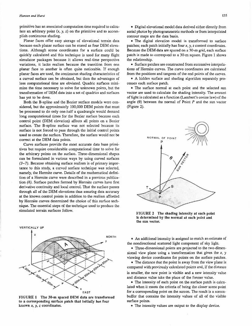
• The surface normal at each point and the selected sun vector are used to calculate the shading intensity. The amount of light is calculated as a function (Lambert's cosine law) of the angle (0) between the normal of Point P and the sun vector (Figure 2).

NORMAL OF POINT

p

FIGURE 2 The shading Intensity at each point is determined by the normal at each point and the sun vector.

• An additional intensity is assigned to match an estimate of the nondirectional scattered light component of sky light.

• Three-dimensional points are projected to the two-dimen­sional view plane using a transformation that gives the x, y viewing device coordinates for points on the surface patches.

• The distance that the point is away from the view plane is compared with previously calculated points and, if the distance

is smaller, the new point is visible and a new intensity value and distance value take the place of the former value.

• The intensity of each point on the surface patch is calcu­lated when it meets the criteria of being the closer scene point for a corresponding point on the screen. The result is a screen­buffer that contains the intensity values of all of the visible surface points.

• The intensity values are output to the display device.

136

EQUIPMENT AND DATA PROCESSING

The Digital Equipment Corporation VAX 11(780 with a VMS operating system was used for computation. Screen output was to a Vectrix VX384. All programs were written in FORTRAN 77. Processing times va...-y according to t.li.e portion of the DEM data quadrangle selected. It takes about 10 min to process approximacely 100,000 DEM data points, which cover 78 km2

(30 mi\ It is estimated that reprogramming and incorporating some new computational efficiencies could reduce processing time to 2 to 3 min for a similar scene.

The Vectrix VX384 display device has a resolution of 672 by 480 pixels. Although this device is capable of producing a multitude of colors, for this study only one selected color was used for land surface thus allowing shading and perspective to impart realism to a scene. The appearance of water bodies in some example scenes illustrates how various colors might be used to enhance visual realism or to possibly accent certain elevational zones.

All of the examples shown are produced from photographs of the Vectrix screen. Such techniques as writing to film can be employed to produce high-resolution images.

TERRAIN MODEL EXAMPLES AND COMPARISONS

The value of a terrain model may be measured by how well it depicts the topography of an area. As a comparison, a black­and-white copy of a color infrared photograph covering the land area of the most northerly 38 percent of the 7.5-min series Rockwood quadrangle is shown in Figure 3. The simulated terrain model for this same area is shown in Figure 4. This model simulates a high oblique view angle from due south and

TRANSPORTATION RESEARCH RECORD 1119

uses lighting from the east to produce an early morning-ap­pearing scene. Note how easily the Cumberland Escarpment is seen running northeast from the western boundary of the model. An inlet from the Tennessee River appears at the center lower edge of the simulated scene.

The three-dimensional-appearing view of the area facilitates locating possible routes over the Cumberland Escarpment. A route closely matching the existing route over the escarpment would probably be chosen by most planners given only the terrain surface model (Figure 4) together with guide instruc­tions to advantageously use passes, saddles, and lead-in ridges to gain elevation. No vertical exaggeration was used on any of the models shown, but any desired vertical exaggeration may be employed for greater terrain emphasis. This surface model is based on ap~roximately 75,000 DEM data points and covers about 59 km (23 mi\

Figure 5 is a simulated vertical view of the Rockwood area and the Cumberland Escarpment. Late afternoon sun from the west is simulated and DLG data of roads are superimposed on the DEM model. The basis of simulation is approximately 100,000 DEM data points covering about one-half of the Rock­wood quadrangle (30 mi2). US-70 ascends the upper portion of the escarpment as shown on the model. The Tennessee River is shown in the lower portion of the model. Simulated terrain surfaces using brown for land areas and blue for water bodies overlaid with white roads are excellent for planning. Conver­sion to black-and-white images greatly degrades the terrain details and the road line sharpness as Figures 5 and 6 indicate. Examination of the model with overlaid roads reveals the general northeast direction of roads dictated by the major topography of the region. The placement of the roads in rela­tion to relief details and water bodies appears to be accurate. However, the use of the road information derived from DLG data would be greatly improved if some method were used to

~

FIGURE 3 Aerial photograph of the upper portion of the Rockwood quadrangle shows the Cumberland Escarpment running northeast on the left side of the photo and the city of Rockwood, Tennessee, in the upper central portion of the photo.

Hansen and Hurst 137

FIGURE 4 A simulated oblique view terrain surface of the Rockwood area and the Cumberland Escarpment has a view angle from the south and simulated early morning lighting.

designate the relative importance of roads. The assignment of identifiers to given line segments is best done at the time of road digitization.

Figure 6 shows a smaller portion of the Rockwood quad­rangle covering 25 km2 (IO mil. Detail is improved on this terrain model because the number of DEMs that make up the

scene is approximately 30,000 compared with the 100,000 DEMs included in Figure 5. This means that, because there are fewer surface patches, more points on each patch can be used and an intensity value for each point calculated. The number of points projected to the screen-buffer must be great enough to impart an intensity to each pixel on the screen so that pixel

FIGURE 5 A simulated vertical view terrain surface of the Rockwood area, the Cumberland Escarpment, and the Tennessee River has simulated late afternoon lighting and is overlaid with the road network of the area.

138 TRANSPORTATION RESEARCH RECORD 1119

FIGURE 6 Smaller portions of the digital elevation model may be selected as the basis of simulating ierrain; titis results in greater surface detaii.

number is constant for a screen device. Because the number of screen pixels is a function of the graphics output CRT, it is easy to see that elevational detail is enhanced by selecting smaller land areas (fewer DEM data points) for a terrain model so that each surface patch (30-m by 30-m ground distance) is de­scribed by more points on each surface. Note is made of the degree to which the location of roads agrees with the perceived relief.

The largest scale simulation done (not shown), which com­prises approximately 11,000 DEM data points and covers an

area of about 10 km2 (4 mi2), may define the limits of large­scale simulation with the USGS DEM data and the equipment used in this study. Close examination of the color slide copy of the Vectrix CRT output of this terrain simulation shows a tendency toward a blocky pattern probably imparted in part by the 30-m square spacing of the DEM data, inaccuracies of the digital data bases, and the effects of a three-dimensional scene being output to a two-dimensional screen. Automated pho­togrammetric elevational equipment often records the elevation of the top of objects and vegetation, which contributes to some of the blockiness. This blocky effect can be seen on a slide with a scale of 1:130,000 when observed with a lOx hand lens. Projection of the slide image confirms this observation.

CONCLUSIONS

Simulated terrain models based on DEM data can be used advantageously in the planning process wherever topography is an element to be considered. The addition of DLG data, trans­portation information, and other boundary information as a line

overlay to the simulated terrain models increases the planning value of such displays and makes them especially useful for public hearings. The ability to select limited land areas and to realistically depict these areas as viewed from any selected vantage point with selected lighting direction is a powerful tool for transportation and land planners.

REFERENCES

1. A. K. Turner. Computer-Assisted Procedures to Generate and Evaluate Regional Highway AlternaJives. Joint Highway Research Project, Final Report 32. Purdue University, West Lafayette, Ind., 1968, 281 pp.

2. J. H. Hansen and M. J. Hurst. Digital Techniques for Terrain Sim­ulation. Proc., Fall Convention, American Society of Photogram­metry and Remote Sensing, Anchorage, Alaska, 1986.

3. B. Barsky. A Description and Evaluation of Various 3-D Models. IEEE Computer Graphics and Applications, Vol. 4, No. 1, Jan. 1984, pp. 38-52.

4. C. Brown and D. Ballard. Computer Vision. Prentice-Hall, Inc., Englewood Cliffs, N.J., 1982.

5. J. li'oley and A. Van Dam. Fundamentals of Interactive Computer Graphics. Addison-Wesley, Reading, Mass., 1982.

6. R. Marshall, R. Wilson, and W. Carlson. Procedure Models for Generating Three-Dimensional Terrain. Computer Graphics, Vol. 14, No. 3, July 1980, pp. 154-162.

7. M. Pratt and I. Faux. Computational Geometry for Design and Manr(acture. Ellis-Horwood Limited, Chichester, England, 1979.

8. M. Hurst. Terrain SimulaJion of United States Geological Survey Digital Elevation Models. M.S. thesis. The University of Ten­nessee, Knoxville, 1985, 59 pp.

Publication of this paper sponsored by Committee on Photogrammetry and Aerial Surveys.