TERAHERTZ COMMUNICATION FOR SATELLITE NETWORKS

TERAHERTZ COMMUNICATION FOR SATELLITE NETWORKS

by

Pulkit Hanswal

June 1, 2018

A thesis submitted to the

Faculty of the Graduate School of the University at Bufalo, State University of New York

in partial fulfllment of the requirements for the

degree of

Master of Science

Department of Electrical Engineering

Copyright by

Pulkit Hanswal

○c 2018

ii

Acknowledgements

I would like to express my sincere gratitude to my advisor Dr. Josep M. Jornet

for the continuous support during my Master thesis and related research, for his

patience, motivation and immense knowledge. The door to Dr. Josep M. Jornet

ofce was always open whenever i ran into a trouble spot or had a question about

my research or writing. His guidance helped me in all the time of research and

writing of this thesis. I could not have imagined having a better advisor and

mentor for my Master thesis.

Besides my advisor, I would like to thank Dr. Elena Bernal Mor for her

encouragement, advise throughout my years of study and recommending me for

the Master thesis to Dr. Josep M. Jornet.

Finally, I must express my profound gratitude to my parents for providing

me with unfailing support and continuous encouragement. This accomplishment

would not have been possible without them.

iii

Contents

Acknowledgements iii

List of Figures viii

List of Tables ix

Abstract x

1 Introduction 1

1.1 Basic Characteristics of Satellites . . . . . . . . . . . . . . . . . . . 1

1.1.1 System Elements . . . . . . . . . . . . . . . . . . . . . . . . 2

1.1.2 Types of Satellite Services . . . . . . . . . . . . . . . . . . . 4

1.1.3 Benefts of Satellite Communication . . . . . . . . . . . . . 7

1.1.4 Frequency Spectrum Allocations . . . . . . . . . . . . . . . 8

1.2 Satellite Classifcation . . . . . . . . . . . . . . . . . . . . . . . . . 9

1.2.1 GEO Satellites . . . . . . . . . . . . . . . . . . . . . . . . . 10

1.2.2 LEO Satellites . . . . . . . . . . . . . . . . . . . . . . . . . 12

1.2.3 MEO Satellites . . . . . . . . . . . . . . . . . . . . . . . . . 13

1.3 Inter-Satellite Communication . . . . . . . . . . . . . . . . . . . . . 14

1.3.1 ISL Frequency Bands . . . . . . . . . . . . . . . . . . . . . 15

1.4 Terahertz Based ISL . . . . . . . . . . . . . . . . . . . . . . . . . . 18

iv

Contents Contents

1.4.1 Terahertz Communication . . . . . . . . . . . . . . . . . . . 18

1.4.2 Summary of Contributions . . . . . . . . . . . . . . . . . . 19

2 Terahertz Wave Propagation in ISL 20

2.1 Spreading Loss . . . . . . . . . . . . . . . . . . . . . . . . . . . . . 20

2.2 Absorption Loss . . . . . . . . . . . . . . . . . . . . . . . . . . . . 22

2.3 Scattering Loss . . . . . . . . . . . . . . . . . . . . . . . . . . . . . 26

2.4 Fading Loss . . . . . . . . . . . . . . . . . . . . . . . . . . . . . . . 28

3 Noise in Terahertz based ISL 30

3.1 Thermal Noise . . . . . . . . . . . . . . . . . . . . . . . . . . . . . 30

3.2 Transceiver Noise Sources . . . . . . . . . . . . . . . . . . . . . . . 31

3.2.1 Amplifer Noise Temperature . . . . . . . . . . . . . . . . . 31

3.2.2 Amplifers in Cascade . . . . . . . . . . . . . . . . . . . . . 33

3.2.3 Noise Temperature of Absorptive Networks . . . . . . . . . 34

3.3 Antenna Temperature . . . . . . . . . . . . . . . . . . . . . . . . . 35

3.3.1 Brightness Temperature . . . . . . . . . . . . . . . . . . . . 36

3.3.2 Cosmic Microwave Background Radiation . . . . . . . . . . 37

3.3.3 Thermal Radiation . . . . . . . . . . . . . . . . . . . . . . . 38

3.3.4 Sky Noise . . . . . . . . . . . . . . . . . . . . . . . . . . . . 38

3.4 Total System Noise . . . . . . . . . . . . . . . . . . . . . . . . . . . 40

3.5 Signal-to-Noise ratio . . . . . . . . . . . . . . . . . . . . . . . . . . 41

4 Link Budget Analysis 43

4.1 Antenna Gain Required - Lower Bound . . . . . . . . . . . . . . . 44

4.2 Antenna Gain Required - Upper Bound . . . . . . . . . . . . . . . 48

4.3 Terahertz ISL vs Optical ISL . . . . . . . . . . . . . . . . . . . . . 50

5 Additional Challenges in THz based ISL 53

5.1 Space Debris . . . . . . . . . . . . . . . . . . . . . . . . . . . . . . 53

v

Contents Contents

5.1.1 System Model . . . . . . . . . . . . . . . . . . . . . . . . . . 54

5.1.2 Simulation Model . . . . . . . . . . . . . . . . . . . . . . . . 55

5.1.3 Power Delay profle . . . . . . . . . . . . . . . . . . . . . . . 58

5.2 Doppler Spread . . . . . . . . . . . . . . . . . . . . . . . . . . . . . 59

6 Conclusions and Future Work 62

Bibliography 63

vi

List of Figures

1.1 Elements of the space segment [1] . . . . . . . . . . . . . . . . . . . 2

1.2 Ground segment [1] . . . . . . . . . . . . . . . . . . . . . . . . . . . 3

1.3 Satellite Links . . . . . . . . . . . . . . . . . . . . . . . . . . . . . . 4

1.4 Fixed satellite service [2] . . . . . . . . . . . . . . . . . . . . . . . . 5

1.5 Broadcasting satellite service [2] . . . . . . . . . . . . . . . . . . . 5

1.6 Mobile satellite service [28] . . . . . . . . . . . . . . . . . . . . . . 6

1.7 GPS constellation [29] . . . . . . . . . . . . . . . . . . . . . . . . . 7

1.8 Inclination classifcation [30] . . . . . . . . . . . . . . . . . . . . . . 9

1.9 LEO,MEO and GEO.Only one orbit per altitude is illustrated,

even though LEO and MEO satellites require multiple orbits for

continuous service [2] . . . . . . . . . . . . . . . . . . . . . . . . . . 10

1.10 GEO satellite system [2] . . . . . . . . . . . . . . . . . . . . . . . . 11

1.11 Iridium constellation [31] . . . . . . . . . . . . . . . . . . . . . . . 13

1.12 TDRS system [32] . . . . . . . . . . . . . . . . . . . . . . . . . . . 15

1.13 RF based ISL [35] . . . . . . . . . . . . . . . . . . . . . . . . . . . 16

1.14 Optical communication based ISL [33] . . . . . . . . . . . . . . . . 18

2.1 THz wave propagation from an elemental antenna [1] . . . . . . . . 21

2.2 Diagram of atmospheric windows [34] . . . . . . . . . . . . . . . . 23

2.3 Absorption loss at THz frequency due to water vapor in dB/km . . 24

vii

List of Figures List of Figures

2.4 Layers of atmosphere [11] . . . . . . . . . . . . . . . . . . . . . . . 26

3.1 Non ideal resistor & its equivalent scheme [1] . . . . . . . . . . . . 31

3.2 Non ideal LNA & its equivalent scheme [1] . . . . . . . . . . . . . . 32

3.3 LNA in cascade [2] . . . . . . . . . . . . . . . . . . . . . . . . . . . 33

3.4 Large bright noise source with brightness temperature �� [2] . . . 36

3.5 Small bright noise source [2] . . . . . . . . . . . . . . . . . . . . . . 37

3.6 Antenna temperature of an ideal ground based antenna. The an-

tenna is assumed to have very low beamwidth without losses and

sidelobes [2] . . . . . . . . . . . . . . . . . . . . . . . . . . . . . . . 39

4.1 Gain required for SNR of 10 dB vs Distance (Lower Bound) . . . . 45

4.2 Beamwidth vs Distance (Lower Bound) . . . . . . . . . . . . . . . 46

4.3 Beam diameter vs Distance (Lower Bound) . . . . . . . . . . . . . 47

4.4 Gain required for SNR of 10 dB vs Distance (Upper Bound) . . . . 48

4.5 Beamwidth vs Distance (Upper Bound) . . . . . . . . . . . . . . . 49

4.6 Beam diameter vs Distance (Upper Bound) . . . . . . . . . . . . . 49

4.7 Beam diameter in Optical ISL . . . . . . . . . . . . . . . . . . . . . 51

4.8 Optical ISL vs THz ISL . . . . . . . . . . . . . . . . . . . . . . . . 52

5.1 Geometry of the Network considered. Refection occuring at point A. 55

5.2 Space debris enclosed in Transmit & Receive Beam,� = 10-9 per �2 56

5.3 Multipath components as function of path delay, � = 10-9 per �2 . 57

5.4 Power delay profle vs time . . . . . . . . . . . . . . . . . . . . . . 59

viii

List of Tables

1.1 Frequency band allocations . . . . . . . . . . . . . . . . . . . . . . 9

1.2 Frequency bands for RF based ISL . . . . . . . . . . . . . . . . . . 17

4.1 Parameters - Lower bound . . . . . . . . . . . . . . . . . . . . . . . 44

4.2 Parameters - Upper bound . . . . . . . . . . . . . . . . . . . . . . . 48

ix

Abstract

Satellite communication, no longer a marvel of human space activity, has become

a fact of everyday life. Satellites are used extensively for variety of communication

applications. In recent years, there is growing interest in the feld of satellite

networks which enables a whole new class of missions for navigation, communication

and remote sensing. Consequently, there is need for innovative methodologies to

meet the increasing demand for high speed wireless communication. Terahertz

band communication is envisioned to be the key technology to satisfy the need

for high data rates. Due to the large availability of bandwidth at terahertz band,

wireless terabit per second links are expected to become reality very soon.

The objective of this work is to study the feasibility of using terahertz band for

inter-satellite communication. We have developed a propagation model considering

several impairments which can afect the propagation of terahertz wave in inter-

satellite links. We have also analyzed noise sources which can impact the terahertz

based communication and calculated the efective noise temperature at the satellite

antenna. A link budget analysis to calculate the gain of the antenna required

to maintain the quality of the link is conducted and a comparative analysis

of terahertz based and optical based inter-satellite communication on the basis

of pointing requirements is also done. Lastly, we have addressed some of the

additional challenges that we need to overcome for implementing terahertz based

inter-satellite communication.

x

CHAPTER 1

Introduction

A satellite is a body that moves around another body (usually much larger) in

a mathematically predictable path called an orbit. Satellites orbiting around

earth can revolve either in circular or elliptical path. Satellites are used for many

purposes. Common types include Earth observation satellites, navigation satellites,

communication satellites, weather satellites, and space telescopes.We mainly focus

in this text on communication satellites.

1.1 Basic Characteristics of Satellites

A communication satellite is a repeater satellite orbiting around earth which

enables multiple users with appropriate earth stations to deliver or exchange

information. Two earth stations which are very distant geographically can make

use of communication satellite which can relay and amplify the signals via a

transponder. The source earth station sends a transmission to the satellite. This

is called up-link communication. The satellite transponder then amplifes or relays

the signal and send it down to the destination earth station. This is called the

1

https://telescopes.We

Tracking. telemetry

and command (TT&C) station

"'~

Deployment

,,..__-i-__ ..... ,

'Transfer l orbit

phase

Chapter 1. Introduction 1.1. Basic Characteristics of Satellites

down-link communication.

Figure 1.1: Elements of the space segment [1]

1.1.1 System Elements

A communication satellite system can be divided into two major parts, the space

segment and the ground segment.

Space Segment

The space segment includes the satellite, the launch station and tracking, telemetry

and command (TT&C) station. Figure 1.1 depicts the main elements of the space

segment. Deployment of a satellite in an orbit is accomplished by the help of a

spacecraft manufacturer and launch agency. After the satellite is placed in the

proper orbit, it is vital to monitor the satellite for the duration of its mission. This

task is accomplished by TT&C station (or stations). The TT&C station establishes

a monitor link to provide essential management and control functions for the safe

2


operation of the satellite. The link between the satellite and TT&C station is

usually separate from the link used for user communication.Tracking, telemetry

and control station is specialized earth terminal facility specifcally designed for

the complex operation required to maintain a satellite in orbit.

Ground Segment

The ground segment of the communication satellite system consists of earth stations

that utilize the communication capabilities of space segment. The earth stations

communicate with satellites to meet the communication needs of the user. It is

important to note that the term earth station is an accepted term that include

the communication stations on the ground, in the air (on airplanes), or on the sea

(on ships). Figure 1.2 depicts a typical ground segment; a single satellite is shown

which acts as a relay to establish the links from one earth station to another.

Figure 1.2: Ground segment [1]

It is important to note that depending upon the coverage area of a satellite,

3

• I I - I I ISL


there can be satellite to satellite link in a satellite system. Figure 1.3 depicts

Inter-satellite links (ISL) and Ground-satellite links (GSL).

Figure 1.3: Satellite Links

1.1.2 Types of Satellite Services

Satellite services are broadly categorized into

∙ Fixed-satellite service (FSS) - This is a type of radio communication service

between earth stations at specifc fxed positions. There are many subdivisions

within FSS, e.g., the FSS provide links for telephone networks as well as for

transmitting TV signals to cable companies. Figure 1.4 depicts a typical

example of fxed satellite service.

4


Figure 1.4: Fixed satellite service [2]

∙ Broadcast-satellite service (BSS) - In this service, the signal transmitted

by the satellite is intended mainly for direct broadcast to the home. It is

sometimes referred to as direct broadcast satellite (DBS) service. One of

the most common example of BSS is Direct to Home(DTH) television.As

shown in Figure 1.5, satellite is broadcasting signal to all the users within

the satellite coverage.

Figure 1.5: Broadcasting satellite service [2]

∙ Mobile-satellite service (MSS) - In this type of service there is communication

between mobile earth stations with the help of one or more satellites. MSS

would include land mobile, maritime mobile, and aeronautical mobile. Figure

5

https://television.As


1.6 shows a mobile satellite phone.

Figure 1.6: Mobile satellite service [28]

∙ Navigation satellite service (NSS) - A navigation satellite service uses a net-

work of satellites (typically 18-30 satellites for global coverage) for providing

geo-spatial positioning. An NSS with global coverage is termed as global

navigation satellite system (GNSS). The most famous example of NSS is

United States’ Global Positioniing System (GPS). Figure 1.7 illustrates a

GPS constellation

6

....... ... ' "

.... .. •••

I I \ • -i r • \ "

,, .. "'· .... • ..... .,..#) -~ . ...... ..


Figure 1.7: GPS constellation [29]

∙ Meteorological satellite service - Lastly, satellites are also used for providing

meteorological services such as weather forecast or services for search and

rescue missions.

1.1.3 Benefts of Satellite Communication

The use of the satellites for communication has become a fact of everyday life.

Satellites are used extensively for a variety of communication applications. It is

evidenced by many homes which are equipped with dishes used for the reception

of satellite television. Satellites also form an essential part of telecommunications

systems worldwide, carrying large amounts of data and voice trafc. As mentioned

in [2], some of the advantages of using satellites are as follows

1) Wide Coverage Area (Country, Continent or Globe) - When designed properly,

a satellite can serve region of any size that can see it. However, in terrestrial

systems, the coverage area is limited usually within a country.

2) Independence from Terrestrial Infrastructure - By providing wide coverage area

and acting as repeater station in space, satellite aids in reducing the terrestrial

7


infrastructure. Two earth station far distant geographically can communicate

without any external connections using satellite (or satellites). It becomes really

attractive in remote areas where the terrestrial infrastructure is poor.

3) Uniform Service Characteristics - Footprint of the satellite defnes the service

area of the satellite. As we will discuss later in this chapter, footprint depends

upon the altitude of the satellite. Within the footprint of the satellite, services are

delivered in precisely the same form. However, in terrestrial systems the quality

of the received signal depend upon the location, e.g., remote areas with poor

terrestrial infrastructure does not have good quality of received signal.

4) Wide Bandwidth Availability- The bandwidth allocated for the satellite services

is generally high. As a result, satellite users enjoy ample amount of bandwidth.

Since, there is a direct relationship between bandwidth and data rate. An increase

in bandwidth can enhance the speed of communication.

5) Rapid Installation & Low Cost - As mentioned in [2], once the satellite system is

operational, the earth station in the ground segment can be installed very quickly.

This is because unlike terrestrial system it does not require extensive planning

such as laying down cables and towers throughout the area. Furthermore, the cost

of constructing a single site is quite modest.

1.1.4 Frequency Spectrum Allocations

Frequency allocation to satellite services is a complicated process which requires

planning and coordination. Frequency band allocation is done by the International

Telecommunication Union (ITU), a specialized agency of the United Nations. Table

1.1 lists the frequency bands assigned by ITU for satellite services.

8

L

s

C

X

Ku

Ka

V

Frequency Range 1.535-1.56 GHz DL; 1.635-1.66 GHz UL

2.5-2.54 GHz DL; 2.65-2.69 GHz UL

3.7-4.2 GHz DL; 5.9-6-4 GHz UL

7.25-7.75 GHz DL; 7.9-8.4 GHz UL

10-13 GHz DL; 14-17GHzUL

18-20 GHz DL; 27-31GHzUL

6oGHzDL; 50GHzUL

General Application

MSS,NSS

MSS, Deep space research

FSS

FSS, Earth observation, Meteorological satellite service

FSS,BSS

FSS,BSS

Open band

Orbit

-@ '~~ (3) a. Equatorial-orbit satellite b. Inc lined-orbit satellite c. Polar-orbit satellite

Chapter 1. Introduction 1.2. Satellite Classifcation

Table 1.1: Frequency band allocations

1.2 Satellite Classifcation

There are many ways to classify satellites. Some of them include inclination

classifcation, synchronous classifcation, altitude classifcation.

a) Inclination classifcation - This divides satellites on the basis of inclination with

reference to the equatorial earth plane. Figure 1.8 illustrates the types of satellites

based on inclination classifcation.

Figure 1.8: Inclination classifcation [30]

b) Synchronous classifcation - In this type of classifcation, satellites are divided

on the basis of the synchronization between the orbital period and rotational period

of the earth. A geosynchronous orbit (GSO) satellite has an orbital period equal

to the rotational period of the earth. Geosynchronous orbit (GSO) satellites rotate

9


around the earth at an altitude of 35,786 km. The synchronization of the rotational

and orbital period means that the satellite return to the same position in the sky

after a period of one day. The path of the satellite over the course of one day

depends upon the inclination and eccentricity of the GSO.

c) Altitude classifcation - This divides satellites by their altitude from the earth.

Figure 1.9 provides three classical Earth-orbit schemes. The commonly used

altitude classifcations are Geostationary earth orbit (GEO) satellites, Medium

earth orbit (MEO) satellites and Low earth orbit (LEO) satellites. We mainly

focus in this text on the classifcation based on altitude.

Figure 1.9: LEO,MEO and GEO.Only one orbit per altitude is illustrated, even though LEO and MEO satellites require multiple orbits for continuous service [2]

1.2.1 GEO Satellites

Geostationary earth orbit is a special case of GSO, which is circular and inclined

at 0∘ to Earth’s equatorial plane. Satellites in GEO revolve at an altitude of about

35,786 km. A satellite in a GEO appears always at the the same point in sky to the

observers on the surface. They are mainly used for FSS, BSS and meteorological

satellite service.

10

I/_,,,--------------------------------+

' ---

•.. ~·. ···• ... -,_______ · , __ '-4' )

---------- ·,.:-_ ,// -------------- ________ ,.,..,.


Figure 1.10: GEO satellite system [2]

Advantages

1. Due to very high altitude, GEO satellites have very large coverage area. It

requires only 3 satellites to cover every part of earth. Figure 1.10 shows a

system of three geostationary communication satellites.

2. As GEO satellites have 24 hour view of a particular location, they are highly

desirable for services which require fxed antenna positions, e.g., DTH, TV

and radio broadcasting

3. As the coverage area of GEO satellites is very wide, there is no need of

handing over the signal from one satellite to another.

4. The Doppler spread in communication between satellite and earth station is

minimal as there is no relative motion between them.

Disadvantages

1. Due to large distance from earth, there is a very high latency which makes

it unft for voice and data communications.

2. Due to large footprints we cannot reuse frequency.

3. As we will see in the later chapters, more distance leads to high propagation

loss which eventually leads to poor quality of signal at the receiver.

4. In order to maintain the quality of the link, high transmit power is needed

11


which is a problem for battery powered devices.

1.2.2 LEO Satellites

LEO satellites revolves in geocentric (around earth) orbits ranging in altitude from

180 km – 2000 km (1,200 mi). LEO satellites do not stay in fxed position relative

to the surface, and are only visible for 15 to 20 minutes each pass. They have

rotation period of 90 to 120 minutes, with speed 20000 to 25000 km/h. They are

mainly used for FSS and MSS.

Advantages

1. Due to it’s proximity to earth compared to GEO satellite, there is better

signal strength in comparison to GEO satellites.

2. They need lesser transmit power for communication in comparison to GEO

satellites.

3. There is very low latency of around 10 milliseconds.

4. They have smaller footprints so there can be frequency reuse.

Disadvantages

1. A network of LEO satellites (50-200),which is also known as satellite con-

stellation, is required to cover entire earth because of the small footprint.

There are satellite to satellite links in the case of LEO satellite network for

handing over the information.

2. The lifetime of LEO satellite is shorter than GEO satellites (5-8 years). This

is because of the atmospheric drag which causes gradual orbital deterioration.

3. There is Doppler spread in the communication between LEO satellite and

earth station because of the relative motion between them.

4. There is need for routing from satellite to satellite to base stations for global

12


coverage.

5. There is requirement for a mechanism for correct handover of the signal from

one satellite to another.

Figure 1.11: Iridium constellation [31]

Some of the examples of LEO satellite systems are as follows

∙ Iridium system - It has 66 satellite in 6 LEO orbits which is used to provide

direct worldwide communication, i.e., voice, data paging, fax. Figure 1.11

illustrates an iridium satellite constellation.

∙ Teledesic - It provides fber-optic like (broadband channels, low error rate,

and low delay) communication.It has 288 satellites in 12 LEO polar orbits.

1.2.3 MEO Satellites

MEO satellites revolves in geocentric orbits ranging in altitude from 2000 km –

35,786 km. MEO satellites are visible for much longer periods of time than LEO

satellites, usually between 2 – 8 hours. They are used mainly for NSS.

13

https://communication.It

Chapter 1. Introduction 1.3. Inter-Satellite Communication

Advantages

1. A MEO satellites’ wider footprint and slower movement in comparison to

LEO satellite means fewer satellites are needed in MEO network than in

LEO network. MEO satellite networks also make use of satellite to satellite

links.

2. Shorter time delay and stronger signal than GEO satellite.

3. It requires fewer handover than LEO network.

Disadvantages

1. Delay is about 70-80 milliseconds.

2. Needs higher transmit power than LEO satellites.

A well known example of MEO satellite network is GPS.

∙ GPS comprises of 24 satellites in six orbits. They are used for land, sea

and air navigation to provide time and locations for vehicles and ships. The

satellites are placed in orbit in such a way that minimum four satellites are

visible from any point on the earth.

1.3 Inter-Satellite Communication

Inter-satellite communication is mainly used for providing global coverage with the

help of satellite to satellite links. There are two types of ISL, intra-orbital links

and inter-orbital links. Intra-orbital links connects the satellites on the same orbit

while inter-orbital links connects the satellites on diferent orbits. Inter-satellite

communication becomes a necessity in the case of LEO and MEO satellite networks

because of their smaller footprint and the need for global coverage.Apart from LEO

and MEO satellite networks, they can also be used for communication between

GEO satellite and LEO satellite. An example of such a satellite system is Tracking

14


and Data Relay Satellite system (TDRS). There are 9 Tracking and Data Relay

satellites which sit at about 35,400 km (almost GEO) above the earth.Occasionally,

satellites present in the LEO orbit are unable to pass along their information to

Earth in the case of unclear view of the ground station. In such a case, TDRS

serves as a way to pass along the satellite information. Figure 1.12 illustrates a

TDRS system. Some of the other well known examples of satellite constellations

which make use of ISL are iridium and teledesic. Apart from providing global

coverage, ISL helps considerably in reducing the terrestrial infrastructure. This

is because we need only 1 up-link and 1 down-link per direction for any point to

point communication.

Figure 1.12: TDRS system [32]

1.3.1 ISL Frequency Bands

Currently, there are two types of ISL based upon the technology used for com-

munication between satellites. Radio Frequency (RF) based ISL make use of

microwaves (0.3 GHz-30 GHz) and millimeter waves (30 GHz - 300 GHz) while

15

Ka-band ---~ ---~ ·band --- ------ Iridium Satellites ---...... ', l-band

' ' ' ' -~ ~autical

, I

I I

/ Ka-band

I I I


optical communication based ISL make use of visible spectrum, i.e., wavelength

range of about 390 nm to 700 nm, for communication.

Radio Frequency based ISL

Long term experience with radio equipment developed for space to ground links

makes RF based ISL more easier to implement in space. As described in [7], in

comparison to optical based ISL, RF based ISL appears more reliable. However, due

to less availability of bandwidth the data rate achievable in RF link is lower than

the optical link.As we will see in the later chapters, due to low carrier frequency

RF links can provide omni directional coverage and also has higher beam width

than optical links which reduces the need for highly accurate acquisiton, tracking

and pointing (ATP) subsystem. Although, this high beam width makes RF links

subjected to interference and multi path propagation. Figure 1.13 illustrates an

iridium satellite system which makes use of RF based ISL.

Figure 1.13: RF based ISL [35]

Table 1.2 indicates the frequency bands allocated to RF based ISL by radio

communication regulations. As we will see in chapter 2, these allocations have

been done because of the strong molecular absorption by the atmosphere at these

16


frequencies. Using these frequencies for ISL provide protection against interference

between terrestrial system and satellite network.

Band Frequency Range 22.55 GHz - 23.55 GHz

Ka 24.45 GHz - 24.75 GHz 32 GHz - 33 GHz 59 GHz - 64 GHz V 65 GHz - 71 GHz

Table 1.2: Frequency bands for RF based ISL

Optical Communication based ISL

Optical communication based ISL has the advantage of providing high speed

communication with the data rate of the order of gigabits per second (Gbps).

However, due to high carrier frequency they have very low beam width. As

mentioned in [10], the challenging part in using optical communication for ISL

is the requirement of an highly accurate ATP subsystem for establishing and

maintaining the communication link. In order to maintain a link in optical

communication based ISL, a direct line of sight is required between transmitter

and receiver. The process of maintaining the link becomes even more complex due

to the rapid relative motion between two satellites. Although, the low beam width

of the optical based ISL aids in receiving interference free signal and also reduces

the possibility of interception. They can also be used for communication between

spacecrafts when they reach very short distances with respect to each other which

guarantees very high position accuracy. A well known example of the optical based

ISL is the TDRS system which makes use of laser for communication.

17

Chapter 1. Introduction 1.4. Terahertz Based ISL

Figure 1.14: Optical communication based ISL [33]

1.4 Terahertz Based ISL

1.4.1 Terahertz Communication

Terahertz band (0.1 THz-10 THz) communication is considered to be the key

technology to support the increasing demand for high speed wireless communication

in the recent years. Due to the large availability of bandwidth at THz band, wireless

terabit per second (Tbps) links are expected to become reality very soon. As we will

see in the next chapter, this very large bandwidth comes at the cost of a very high

propagation loss. The high propagation loss is primarily due to the high molecular

absorption at THz frequencies and also due to the increase in spreading loss at

higher frequency. The advancements in the feld of communication can compensate

for the propagation loss at higher frequencies but the high molecular absorption

remains an issue. Consequently, for the time being, THz band communication

in terrestrial environment is mainly constrained to very short (e.g., on chip) and

short (e.g., in a room) links.

18

Chapter 1. Introduction 1.4. Terahertz Based ISL

In this work, we propose satellite to satellite links using THz frequencies. Due

to the high availability of bandwidth, THz based ISL can enable higher data

rate in comparison to RF based ISL without having to switch to a diferent set

of hardware such as lasers for optical communication. Also, due to the high

frequency of the communication system, the size of the antenna required for THz

based ISL is very less which is highly favorable to the smaller satellite systems.

Terahertz spectrum also provides inherent isolation from terrestrial RF systems

and thus eliminates potential radio frequency interference from ground systems.

Furthermore, as explained in [7], because of the presence of multiple GHz channel

bandwidth terahertz wireless system has very low complexity system design with

simplest modulation schemes in comparison to traditional radio architectures.As

we will show in the future chapters, THz based inter-satellite communication also

have higher efciency than optical communication based ISL.

1.4.2 Summary of Contributions

In the following chapters, we will develop a propagation model and learn about

the factors afecting the THz wave propagation in ISL. In Chapter 3, we will look

into the noise sources which can afect THz based inter-satellite communication.

In Chapter 4, we will conduct a link budget analysis and do a comparative study

between optical and terahertz based ISL. Finally, we will address some of the major

challenges that we need to overcome for implementing THz based inter-satellite

communication.

19

https://architectures.As

CHAPTER 2

Terahertz Wave Propagation in ISL

When a THz wave propagates through a medium there can be several impairments.

Some of the important impairments which afect THz wave propagation will be

described in this chapter.

2.1 Spreading Loss

Spreading loss indicates the amount of power that is lost when an EM wave

propagates in an environment. Once THz wave is several dimensions away from

its emitter, its energy propagates out radially. Figure 2.1 depicts THz wave

propagation from an elemental antenna.

20

Maximum propagation

Antenna reference

axis ' ' ' : '

I I I I I I I I I I I

Maximum propagation

Chapter 2. Terahertz Wave Propagation in ISL 2.1. Spreading Loss

Figure 2.1: THz wave propagation from an elemental antenna [1]

Consider an isotropic point source with a transmitting power of ��. At a

distance d from the source, the radiated power is uniformly distributed over the

surface area of a sphere.

We can write the received power �� at distance d is given by

1 �� = �� (2.1)4��2

��,

where �� is gain of the transmitter antenna and �� is the efective aperture of the

receiver antenna. We can also write the gain of the receiver antenna �� by

�� =4 �

� 2

��, (2.2)

where � is the wavelength of the THz wave.

After substitution we get,

( )2�

�� = �� , (2.3)4��

which we can further rewrite to

( )2�

�� = �� , (2.4)4��

21

Chapter 2. Terahertz Wave Propagation in ISL 2.2. Absorption Loss

where c is the speed at which THz wave propagates in a medium & �� is the carrier

frequency of the wave. The spreading loss is given by

( )21 4�� = . (2.5)

��

We can further express this equation in decibels(dB).

�� = �� + �� + �� − �� . (2.6)

The propagation model described by equation (2.6) is known as Friis prop-

agation model. From equation (2.5) we can see that as we increase the carrier

frequency the power received at the receiver antenna decreases. This equation

explains the cause of high spreading loss, when communicating at THz frequencies.

We can also see that this spreading loss can be compensated by increasing the

gain of the receiver and transmitter antennas. The propagation loss also increases

as we increase the distance between transmitter and receiver. The propagation

model described above is also known as free-space model. This model very well

fts our scenario. We will be using this model to conduct link-budget analysis in

the Chapter 4.

2.2 Absorption Loss

Atmospheric absorption of electromagnetic radiation happens when the energy of

the photon present in the radiation is taken by the molecules (typically electrons of

atom) in the atmosphere. This electromagnetic energy absorbed by the molecules

is usually converted into another form such as thermal energy. Figure 2.2 illustrates

the wavelengths at which the EM waves are note able to penetrate the Earth’s

atmosphere. The primary gases which leads to atmospheric absorption of energy

are water vapor, ozone and carbon dioxide. As shown in Figure 2.2, the wavelengths

22

-~

:1 ,]MC:i f {f .. 0 <> EO <

I I I I I I 01 nm 1"m 10nm 100nm

Gamma Raya, X•Raya and Ultrav ic»et Llgh1 blocked by the upl)ef • 1mOSl)hefe (b .. 1 obHrvttd from apace).

1 ,m 101,1m

Viaibk Ligh1 observable f rom Earth, wi1h some •tmospheric distortion.

1001,1m 1 mm 'cm Wavelength

Mos1ot the lnfrarttd ap.tetrum • bsorbed by abnospheric gasses (bes1 -~ ... from space).

10cm 1m 10 m

Radio W.Vff observable from Earth.

I I 100m 1 km

Long-wavelength R.ldio Wav .. blocked.


in the range of 30 �m to 3000 �m (Terahertz range) are completely absorbed by

Earth’s atmosphere.This absorption is mainly due to the water vapor present in

the atmosphere.

Figure 2.2: Diagram of atmospheric windows [34]

Figure 2.3 shows attenuation due to water vapor in the range of 0.1 THz

to 10 THz. It shows that the attenuation can go as high as 1000 dB for some

specifc frequencies. Due to this very strong absorption we are unable to use THz

frequencies for terrestrial systems.

23

1800

1600

I 1400 ii3 ~ 1200 <JJ

gi ..J 1000 C 0

li 800

~ .n <x: 600

400

200

2 3 4 5 6 8 9 10

Frequency ITHz]


Figure 2.3: Absorption loss at THz frequency due to water vapor in dB/km

Layers of Earth’s Atmosphere

In order to analyze the impact of atmospheric absorption on THz based ISL, we

should frst study about the layers of atmosphere. Earth’s atmosphere consists

of series of layers each of which has its own properties. Moving upward from

the ground level, these layer are named as troposphere, stratosphere, mesosphere,

thermosphere and exosphere. Figure 2.4 depicts all the layers of atmosphere.

∙ Troposphere - The troposphere is the lowest layer of the atmosphere. It

extends upward from ground level to about 10 km (33,000 feet) above sea

level. 99% of the water vapor in the atmosphere is found in the troposphere.

As we move up in the troposphere temperature gets colder.

∙ Stratosphere - The stratosphere extends from the top of troposphere to about

50 km above the ground. This layer contains the ozone molecules which

absorb the high-energy ultraviolet (UV) light from the Sun, which is then

converted into thermal energy. The temperature of the stratosphere gets

24


warmer as we move upwards.

∙ Mesosphere - The next layer up is called mesosphere. It extends upward to

a height of about 85 km above earth. Unlike the stratosphere, temperature

once again grows colder as we rise up through the mesosphere. The top of

the mesosphere is the coldest place in earth’s atmosphere with a temperature

around -85∘C (188∘K). The air density in mesosphere is far too low to breathe.

Also, the air pressure at the bottom of the mesosphere is 1% of the pressure

at sea level.

∙ Thermosphere - Above the mesosphere is the thermosphere. As mentioned

in [11], this layer is completely free of water vapor. High energy X-rays and

UV radiation from the Sun are absorbed in the thermosphere. As a result,

temperature of the thermosphere can range from about 500∘C (773∘K) to

2000∘C (2273∘K). However, as we will see in the next chapter, due to very

low density of the air the notion of the temperature is not meaningful at this

layer. The top of the thermosphere lies between 500 to 1000 km depending

upon the amount of the radiation coming from the sun. LEO and many

MEO satellites orbit at this layer.

∙ Exosphere - The exosphere is the topmost layer of the atmosphere.The air is

very, very thin at this layer of the atmosphere. The top of the exosphere lies

at about 10000 km after which it fnally fades into space. This layer is also

completely free of water vapor.

25

Chapter 2. Terahertz Wave Propagation in ISL 2.3. Scattering Loss

Figure 2.4: Layers of atmosphere [11]

As mentioned above, layers thermosphere and exosphere of the atmosphere

does not contain any amount of water vapor. Figure 2.3 shows the impact of

water vapor on THz frequencies. Since LEO & MEO satellites are present at the

thermosphere and exosphere layer of the atmosphere while GEO satellites are

present in deep space, we can say that in THz based ISL the absorption of the

THz frequencies will be negligible. Thus, absorption will not have a considerable

afect on THz based ISL.

2.3 Scattering Loss

Scattering is a process in which some forms of radiation, such as light, change its

path from straight trajectory into one or more paths. Scattering occurs due to the

deformities present in the material medium through which the EM wave pass.

It is important to understand that refection, refraction and scattering all leads

26

Chapter 2. Terahertz Wave Propagation in ISL 2.3. Scattering Loss

to the re-direction of light. When the medium is uniform and homogeneous over

lengths that are much larger than the wavelength then a well-defned direction of

propagation emerges. This is refraction. However, when the medium is smaller or

comparable to the wavelength then the wave goes of in diferent direction. This

is scattering.We can say that refraction is a form a scattering. Scattering of the

electromagnetic waves corresponds to the collision and scattering of a wave with

some material object.

Types of Scattering

Depending upon the size of the material object with which the EM wave colloids,

scattering can be categorized into three.

∙ Rayleigh Scattering – This occurs when the size of particle is small in

comparison to the wavelength of the wave.

∙ Mie Scattering – This type of scattering occurs when particle is about the

same size as wavelength of the wave

∙ Geometric Scattering – This is caused when the particle is much larger than

the wavelength of wave

In order to do the analysis of the impact of scattering on THz Based Inter-satellite

communication, we should frst analyze the type of scattering which occurs at the

layers where satellites are present.

In case of optical/laser communication geometric scattering is mainly caused by

rain droplets and snow [15]. Aerosol particles,fog and haze are major contributors of

mie scattering [14] while rayleigh scattering is mainly caused by air molecules [16].

As we discussed above, in thermosphere and exosphere the only thing which is

present is air molecules with very low density. Now, in our scenario we are trans-

mitting at THz frequency which means at higher wavelength than the wavelength

27

https://scattering.We

Chapter 2. Terahertz Wave Propagation in ISL 2.4. Fading Loss

used in optical communication. So, we can infer that only scattering which is

possible in THz based ISL is rayleigh scattering.

In the case of rayleigh scattering the relation between amount of scattering

and wavelength is given by [13]

1 � ∝ (2.7)

�4 ,

where � is the wavelength of the THz wave and I is the intensity of the light

scattered

As described in [12], rayleigh scattering is neglected at wavelengths in the near

infrared range (0.75 �m-1.4 �m). In THz based ISL,we are transmitting at

wavelengths higher than the wavelength in the near infrared range. Due to the

inverse relationship shown in equation (2.7), the impact of scattering in THz

based ISL is even lesser in comparison to the scattering in near infrared range.

Furthermore, the density of the air molecules in the upper layers of the atmosphere

is very less.Thus,we can conclude that when we are using terahertz band for inter

satellite communication there cannot be huge impact on the signal quality due to

scattering.

2.4 Fading Loss

There are mainly three mechanisms through which an EM wave propagate in a

terrestrial wireless medium; refection, which is a type of geometric scattering,

difraction and rayleigh scattering.These mechanisms lead to arrival of multiple

electromagnetic waves at the receiver at the same time. These waves usually arrive

at receiver from diferent directions and experience diferent delay due to traversing

unequal distances. The received signal amplitude and phase of each of the wave

can difer as they travel diferent distances. As a result, these EM waves can add

28

Chapter 2. Terahertz Wave Propagation in ISL 2.4. Fading Loss

either constructively or destructively. Due to this, we can observe fuctuations

in the received signal power. Furthermore, the received signal can vary rapidly

in phase and amplitude if there is relative motion between the transmitter and

receiver.

When an EM wave propagates from transmitter to receiver, signal sufers one

or more refections.This leads to multi path propagation. Due to unequal distances,

time of arrival of each path at the receiver is diferent. This leads to spreading out

of the signal in time. This spread is called as delay spread. As we will discuss in

the future chapter, high delay spread can lead to inter symbol interference.

Fading also occurs when there is relative motion between transmitter and re-

ceiver. Due to doppler efect, relative motion leads to generation of new frequencies

at the receiver. In chapter 5, we will see that high speed of the transmitter or

receiver can lead to very rapid change in the channel response causing distortion

in the received signal.

29

CHAPTER 3

Noise in Terahertz based ISL

Noise is an unwanted disturbance that gets added during the capturing or processing

of the desired signal. In this chapter we will mainly look at the type of noise in

free space and analyze their impact on THz based inter satellite communication.

3.1 Thermal Noise

Thermal noise is the electronic noise generated by the motion of the charged

particles such as electrons inside an electrical conductor. Except at absolute zero

temperature, the electrons in every conductor (resistor) are always in thermal

motion. This noise is generated even when there is no voltage applied to the

conductor. This motion leads to voltage diference between the resistor’s terminal.

As shown in Figure 3.1, this can be modeled as resistor with the noise source.

30

R (rhy~-.s.1) kTB - (id&I)

Chapter 3. Noise in Terahertz based ISL 3.2. Transceiver Noise Sources

Figure 3.1: Non ideal resistor & its equivalent scheme [1]

As mentioned in [2], if this resistor is connected to a matched load the thermal

noise delivered by the noise source will be equal to

�� = �� , (3.1)

where K is the Boltzmann constant in Joules per Kelvin (� = 1.38 × 10−23 J/ K),

T is temperature in kelvin and B denotes bandwidth in Hz.

We can use equation (3.1) to defne an efective noise temperature for the other

noise sources too, even if the origin of the noise is not thermal. Any noise source

having a noise temperature of �� will generate thermal noise equal to a resistor

at temperature ��. It is very important to note that, unlike resistors noise

temperature of any noise source is not always equal to its physical temperature.

3.2 Transceiver Noise Sources

In this section we will defne noise fgure and see the efective noise temperature of

some of circuit components important to our analysis.

3.2.1 Amplifer Noise Temperature

As discussed in Sec.3.1, we can defne efective noise temperature for any type

of noise source. Consider a non ideal low noise amplifer (LNA) with gain G. As

31


shown in Figure 3.2, this amplifer has input signal �� with some noise ��. Apart

from ��, this amplifer will add some extra noise to the signal. As described in

Sec.3.1, in a similar way this amplifer can be replaced by an ideal amplifer and

an artifcial noise source ��.

Figure 3.2: Non ideal LNA & its equivalent scheme [1]

Noise Factor

The noise factor is defned as the signal-to-noise ratio between input and output of

the system. The noise factor of the LNA described in Figure 3.2 can be given by

�� = 1 + ��

� = (3.2)��

In order to make it possible to compare diferent amplifers, noise fgure is calculated

by keeping a reference temperature of 290 K. This artifcial noise can now be

thought of as fxed. At a temperature of 290K,the value of the noise power per

unit hertz can be given by

�0 = ��0 = 1.38 × 10−23 × 290 = 4 × 10−23�/��. (3.3)

The noise fgure is simply F expressed in decibel [1]

�� = 10��10�. (3.4)

32

Ampliriief l I Ampiifie r 2 -G, Na. ;i G2 T~1 T,12 .__

!

No.1


Noise Temperature

As we can see from equation (3.3) the value of noise power is very low. Sometimes

it becomes to difcult to deal with these small values. We can rewrite equation

(3.2) to

= 1 + ��

� , (3.5)�0

which can be be further rewritten to

�� = (� − 1)�0 = (� − 1) × 290, (3.6)

where �� denotes the efective temperature noise of the LNA, �0 is the reference

temperature (290K) and F is the noise fgure.

3.2.2 Amplifers in Cascade

It is possible to calculate the efective noise temperature of the amplifer connected

in cascade. The cascade connection is shown in Figure 3.3 The overall gain is

� = �1�2. (3.7)

Figure 3.3: LNA in cascade [2]

33


System noise temperature in this case can be given by [2]

��2�� = ��1 + , (3.8)

�1

where �� is the system noise temperature, ��1 is the noise temperature of the frst

amplifer, �1 is the gain of the frst amplifer and ��2 is the noise temperature of

the second amplifer. Using equation (3.8), the total system noise can be given by

�0,1 = ��. (3.9)

This is a very important result. It shows that in order to have low system noise

temperature, the frst stage should have high power gain as well as low noise

temperature. This result may be generalized to any number of stages in cascade [1].

The system noise temperature of more than two amplifers in cascade can be given

by ��2 ��3

�� = ��1 + + + ... (3.10)�1 �1�2

3.2.3 Noise Temperature of Absorptive Networks

A network which contains resistive elements is considered to be an absorptive

network. Since an absorptive network contains resistance it generates thermal

noise. Transmission lines, feeder lines and waveguides are some of the examples of

the absorptive networks. Feeder line is generally used to connect to the satellite

antenna. The efective noise temperature of an absorptive network is directly

related to the power loss L.

Consider an absorptive network which has a power loss L. The power loss is

the ratio of the input signal power to the output signal power. It is always greater

than unity. From [1], the efective noise temperature of an absorptive network is

34

Chapter 3. Noise in Terahertz based ISL 3.3. Antenna Temperature

given by

�� = (� − 1)��, (3.11)

where �� is the physical temperature. On comparing with equation (3.6), we can

see that if an absorptive network is at room temperature(290K) then its power

loss is equal to its noise factor.

3.3 Antenna Temperature

Antennas operating in the receiving mode introduce noise in the satellite circuit.

The temperature associated with the noise at the terminals of the antenna is known

as antenna temperature. We can think of it as the efective noise temperature of the

antenna. The noise energy due to the antenna temperature is the weighted average

of the noise sources the antenna is looking at. The weighting factor depends upon

the directivity towards a specifc noise source. Antenna temperature is due to

the presence of radiations in the antenna environment and antenna losses. It is

important to note that the antenna temperature is not the physical temperature

of the antenna. The antenna temperature is usually calculated experimentally.

But, it is possible to fnd an upper bound on the antenna temperature depending

upon the scenario.

Under Rayleigh-Jeans approximation (h� << KT), the antenna temperature

is given by ∫∫ 1 �� = �(�, �)�� Ω, (3.12)4� Ω

where �(�, �) is the radiation pattern of the antenna and �� is the brightness

temperature.

35


3.3.1 Brightness Temperature

Brightness temperature is the physical temperature that black body in thermal

equilibrium would have to be in order to radiate the same power as of the non-black

body at a frequency �. Brightness temperature of a body varies with the frequency.

At any temperature and at any frequency, the power radiated by a black body is

more than a non-black body. As a result, the brightness temperature of a noise

source is always less than its physical temperature.

In the case of large bright noise object, the antenna temperature due to the

noise source is equal to its brightness temperature. Figure 3.4 depicts a large

bright noise source with brightness temperature �� . The antenna temperature for

a large bright noise source is independent of the radiation pattern and the distance

between the antenna and noise source.

Figure 3.4: Large bright noise source with brightness temperature �� [2]

However, antenna temperature does depend upon the distance and the radiation

pattern in the case of small bright objects. Figure 3.5 shows a small bright object.

It is very evident from Figure 3.5 that if the distance between the noise source

and antenna changes the solid angle (Ω� ) subtended by the noise source at the

antenna will change. The antenna temperature due to a small bright noise source

36

@·---------~-{-~ ---~,,_( ~~~--:~~~~~~~~:-----------------c~~~.-~ .... --:===--•--


is given by Ω�

�� = �� , (3.13)Ω�

where Ω� is the solid angle of the main lobe of antenna.

Figure 3.5: Small bright noise source [2]

Now we will look at some of the possible noise sources which could contribute

towards antenna temperature in THz based ISL.

3.3.2 Cosmic Microwave Background Radiation

Cosmic Microwave Background Radiation (CMBR) flls the entire universe and

is the leftover radiation from the big bang. According to Big Bang, initially the

universe was flled with hot plasma of particles (protons, neutrons and electrons)

and photons (light). For the frst 380,000 years the photons were interacting

with electrons and were not able to travel long distances. However, the universe

expanded and the temperature came down to 3000 kelvin. Now the protons and

electrons were able to combine to form hydrogen atoms. In the absence of free

electrons, the photons were able to travel more distances and thus the universe

became transparent.Over the billions of years, universe has expanded and cooled

greatly and the temperature has reduced to 2.7 K

In 1989, NASA sent a Cosmic Background Explorer (COBE) to study about

CMBR. The key discovery was that CMBR was found to be extremely precisely to

a so called black body at a temperature of 2.73 K. Since the peak of CMBR lies

37


in the microwave region, the brightness temperature at THz frequencies due to

CMBR is very less. Needless to say, the brightness temperature of CMBR cannot

go above 2.73 K. As a result, the impact of CMBR on THz based ISL is negligible.

3.3.3 Thermal Radiation

Any body above a temperature of 0K, emits out electromagnetic radiation. These

radiation are known as thermal radiation. These radiations are generated due to

the motion of the charged particles in the matter. Some of the examples of thermal

radiation are infrared light and visible light. The peak of the thermal radiation

depends upon the temperature of the object.The peak lies in infrared region at

room temperature (290 K). Thermal radiation from the Earth has considerable

impact on satellite antennas. This is because satellite antennas generally point

towards the earth. As a result, they receive full thermal radiation from it. Since

the size of satellite antenna is very small in comparison to the size of the noise

source, i.e., Earth, the antenna temperature due to the thermal radiation from

Earth is considered to be 290 K which is the physical temperature of the Earth.

3.3.4 Sky Noise

A body which absorbs radiation also emits out radiation. The amount of the

radiation a body emits depends upon the absorptivity of the body. A perfect

black body has emissivity and absorptivity both equal to 1. Consider, e.g., there

is no atmosphere and the antenna at the earth station is pointing towards the

space. In this case the only noise source the antenna is looking at is the cosmic

noise, and the antenna temperature would be 2.7 K. But since the atmosphere

absorbs radiation, it also emits some radiation of its own. These radiation acts

as noise at the antenna and contribute signifcantly to the antenna temperature.

This contribution is known as sky noise. Sky noise depends upon the frequency

38

Galac1ic•r..oise region Lo w.no ise region

10,000 ;::::::::::'.:::::: ::::;.::::::: :::'.:::::::::::;::::::::: :'.:::::::::::::

10

Frequeocv. GHt

resonance 22.2 GHz

100


and the direction at which the antenna is pointing.

Figure 3.6 depicts the antenna temperature due to the sky noise for an earth

station antenna. The lower graph is for the antenna pointing directly overhead

while the upper graph is for the antenna pointing just above the horizon. The

diference between the two curves is due to the thermal radiation from the Earth

at 290 K. When the antenna is pointing to zenith, then antenna temperature is

only due to the sky noise. However, when the antenna points towards the horizon

then due to the thermal radiation from the earth the antenna noise temperature

increases.

Figure 3.6: Antenna temperature of an ideal ground based antenna. The antenna is assumed to have very low beamwidth without losses and sidelobes [2]

Notice the two peaks in the antenna noise temperature above 10 GHz. These

peaks are due to resonant losses in the Earth’s atmosphere by �2��2. In the

case of rainfall,the atmospheric absorption is even more and hence the antenna

noise temperature increases.We can say that rainfall degrades the transmission in

two ways, it attenuates the signal as well as it introduces noise in the system.

39

https://increases.We

Chapter 3. Noise in Terahertz based ISL 3.4. Total System Noise

3.4 Total System Noise

In this section we will calculate the overall system noise temperature.The con-

stituent elements of the receiving satellite are divide into antenna element, the

feeding section (outside the satellite), the feeding section (inside the satellite) and

the receiver (inside the satellite).Using equations (3.6, 3.10, 3.11) and as mentioned

in [26], the total system noise can be given by

�� = �� + (�1 − 1)�1 + �1(�2 − 1)�2 + �1�2(�� − 1)�0, (3.14)

where �� is the antenna temperature, �1, �2, �0 are the physical temperature of the

feeder line (outside the satellite), feeder line (inside the satellite) and the receiver

respectively. �1&�2 are the loss in the feeding section (outside the satellite) and

feeding section (inside the satellite) respectively, and NF is the noise fgure of

the receiver. We will be using this equation to calculate the total noise power

generated in THz based inter-satellite communication.

Now the total noise power �� at the receiver can be readily found as

�� = ��, (3.15)

where K is the boltzman constant and B is the bandwidth.

It is important to note that the temperature outside the satellite depends

upon the location of the satellite in the orbit. In order to fnd the range of the

temperature outside the satellite, we frst need to understand how a body attains

temperature. There are three ways through which heat is transferred from one

body to another.

∙ Conduction - In conduction there is a direct fow of heat through a body as

a result of physical contact from another body. The former body can either

gain or loose heat which can eventually lead to the increase or decrease in

40

Chapter 3. Noise in Terahertz based ISL 3.5. Signal-to-Noise ratio

the temperature of the body.

∙ Convection - In case of convection, heat is transferred to the body by the

fuids such as gas or liquid. Heat transferred to the body by the collisions of

the atmospheric molecules is an example of convection.

∙ Radiation - In radiation mechanism heat is transferred to a body using elec-

tromagnetic wave. It does not require any material medium for transferring

the heat.

In THz based ISL, we will be communicating in an environment where the density

of the air is very low. There will be very less air molecules to transfer the heat

via convection. So even though the temperature of thermosphere is 2000∘C (2273

K), the temperature outside the satellite is very low. Also, the heat transfer will

not take place via conduction as it requires a separate physical body for transfer.

Hence, in our analysis the only way through which heat transfer can take place is

via radiation. As a result, the temperature of LEO satellites vary from -170∘C

(103 K) to 123∘C (396 K) depending upon the location in the orbit. We have to

consider this wide variation in the temperature outside satellite in our link budget

design as it can impact the total noise power at the receiver.

3.5 Signal-to-Noise ratio

The signal-to-noise ratio (SNR) is an important measure to evaluate the perfor-

mance of the satellite link. It is the ratio of carrier power to noise power at the

receiver input. It is given by � �� = , (3.16)� ��

41

Chapter 3. Noise in Terahertz based ISL 3.5. Signal-to-Noise ratio

where �� is the received power and �� is the noise power. This equation can also

be expressed in decibels (dB)

( ) � = �� − �� . (3.17)� ��

� Using equations (2.6, 3.14, 3.17), we can rewrite the ratio as�

( ) � = �� + �� + �� − �� − �� − �� − �� . (3.18)� ��

42

CHAPTER 4

Link Budget Analysis

From the information we have gained from the previous chapters, in this chapter

we will be devising link budget for THz based inter-satellite communication. We

will begin by calculating the gain of the transmitter and receiver antenna required

to compensate for the high propagation loss occurring due to the transmission

at THz frequencies. We will also calculate the beam width corresponding to the

gain, and then we will perform a comparative analysis on the basis of the pointing

requirements between Optical and THz based ISL.

For link budget analysis, we will make use of the Friis Propagation model

developed in Chapter 2. For calculating the noise power we will be making use of

the total system noise temperature equation developed in Chapter 3.

The recent advancements in the terahertz technology, such as III-V semicon-

ductor technologies in an electronic approach and Quantum Cascade Lasers in an

optics approach, allows us to generate frequencies from 0.34 THz to 1 THz with a

power of 1 mW to 10 mW [4, 18].

We will divide the analysis into two parts depending upon the transmit power,

carrier frequency and location of the satellite in the orbit. We desire to achieve an

43

Parameters Value

pt lOmW

{c 0.34THz

TA 300K

L1,L2 1.3 dB

Ti 103K

Tz 290K

NF 3 dB

d so km - 1000 km

B 1 GHz, 5 GHz, 10 GHz

Chapter 4. Link Budget Analysis 4.1. Antenna Gain Required - Lower Bound

SNR of 10 dB at the receiver. At frst, we will fnd the lower bound on the gain

of the antenna required to maintain an SNR of 10 dB at the receiver. We will

do the analysis by choosing three diferent values of the bandwidth. In the same

way, we will be fnding an upper bound on the gain of the antenna with respect to

distance.

4.1 Antenna Gain Required - Lower Bound

For lower bound analysis the temperature outside the satellite is taken to be

-170∘C (103 K). This is because as we decrease the temperature the noise power

decreases and the signal to noise power ratio increases. Hence, we would require

less amount of gain of the antenna to achieve the same SNR.

Table 4.1 indicates the parameters considered in the lower bound analysis.

Table 4.1: Parameters - Lower bound

44

6B Fe= 0.34 THz, Pt= 10 mW, Tsys = 683.1 K

--8=1 GHz 66 ~ B=5GHz ------ - B= tO GHz 64

62 ,,,,, ,,,,,

co / /

~ 60 /

~ /

·~ 5B /

~ I C 56

I ·;;; I 0 I

54 I

52

50

4B 0 100 200 300 400 500 600 700 BOO 900 1000

Distance[km]


Gain Required

Figure 4.1: Gain required for SNR of 10 dB vs Distance (Lower Bound)

From Figure 4.1, we can see that as the distance increases the gain required to

achieve SNR of 10 dB also increases. This is due to the increase in the propagation

loss with the distance. The total system noise temperature is found to be 683.1

K. We can also see that the gain required is the highest in the case when the

bandwidth is 10 GHz. This is because the total noise power is directly proportional

to the bandwidth. As a result, we will need more gain of the antenna to achieve

SNR of 10 dB.

Beamwidth

The beamwidth, also known as half power beamwidth (HPBW), is the angle

between the half power points (-3 dB) of the main lobe. In this section, we

will calculate the upper bound on the HPBW corresponding to the gain of the

transmitter and receiver antenna calculated in previous section. From [20], the

45

Fe= 0.34 THz, Pt= 10 mW, Tsys = 683.1 K 0.8 ~-~-~--~-~--~-~-~--~-~-~

0.7

O.G

ru ~ 0.5 <1> ~ ~ 04

-~ ~ 0.3 co

0.2

0.1 --- - - -

--B=l GHz ~ B=SGHz - - B=lOGHz

---------o~-~-~--~-~--~-~-~--~-~-~

0 100 200 300 400 500 600 700 800 900 1000

Distance[km]


gain of the antenna is related to the half power bam width as

32400 � ≤ , (4.1)

��

where � is horizontal beamwidth in degrees and � is the vertical beamwidth in

degrees. Horizontal and vertical beamwidth are the angles in the horizontal and

vertical plane where the power of the main lobe is reduced by half. We will assume

the horizontal and vertical beam width to be equal in our analysis. The relation

between HPBW and gain of the antenna can now readily found to be

√ 32400

�� = , (4.2)�

where �� is the HPBW in degrees.

Figure 4.2: Beamwidth vs Distance (Lower Bound)

From Figure 4.2 we can see that as the distance between transmitter and

receiver increases the upper bound on the HPBW decreases. This is due to the

46

Fe= 0.34 THz, Pt= 10 mW, Tsys = 683.1 K 3.5 ~-~-~--~-~--~-~-~--~-~-~

3

2.5

I ~ 2 E .!!! ~ 1.5

"' Q)

co

0.5

--8=1 GHz ~ 8=5GHz - - 8=10 GHz

o'--~--~-~--~-~--~-~--~--'---' 0 100 200 300 400 500 600 700 800 900 1000

Distance[km]


inverse relationship between the gain and the HPBW. It is important to note that

as the HPBW decreases it becomes difcult to aim at the receiver. Hence, there is

a need for an accurate pointing system for communicating with the receiver.

Beam Diameter

Using geometry, the beam diameter at a particular distance d of an antenna beam

with HPBW �� can be readily found as

( )

�� = 2��

. (4.3)2

Figure 4.3: Beam diameter vs Distance (Lower Bound)

From Figure 4.3, we can see that the beam diameter is increasing with distance.

It is very important to note that even though the HPBW is decreasing the beam

diameter is increasing and it is of the order of kilometer (km).

47

Parameters Value

pt lmW

fc l THz

TA 300K

L1,Lz 1.3 dB

T1 396K

Tz 290K

NF 3dB

d so km - 1000 km

B 1 GHz, 5 GHz, 10 GHz

78 Fe = 1 THz, Pt= 1 mW, Tsys = 712.4 K

--B=1 GHz 76 -e-e=SGHz ------ - B=lOGHz --74

72 ,,,. iii'

,,,,

~ 70 /

/

~ / -~ 68 / ~ I

~ 66 I

~ I

64 I

I

62

60

58 0 100 200 300 400 500 600 700 800 900 1000

Distance[km]

Chapter 4. Link Budget Analysis 4.2. Antenna Gain Required - Upper Bound

4.2 Antenna Gain Required - Upper Bound

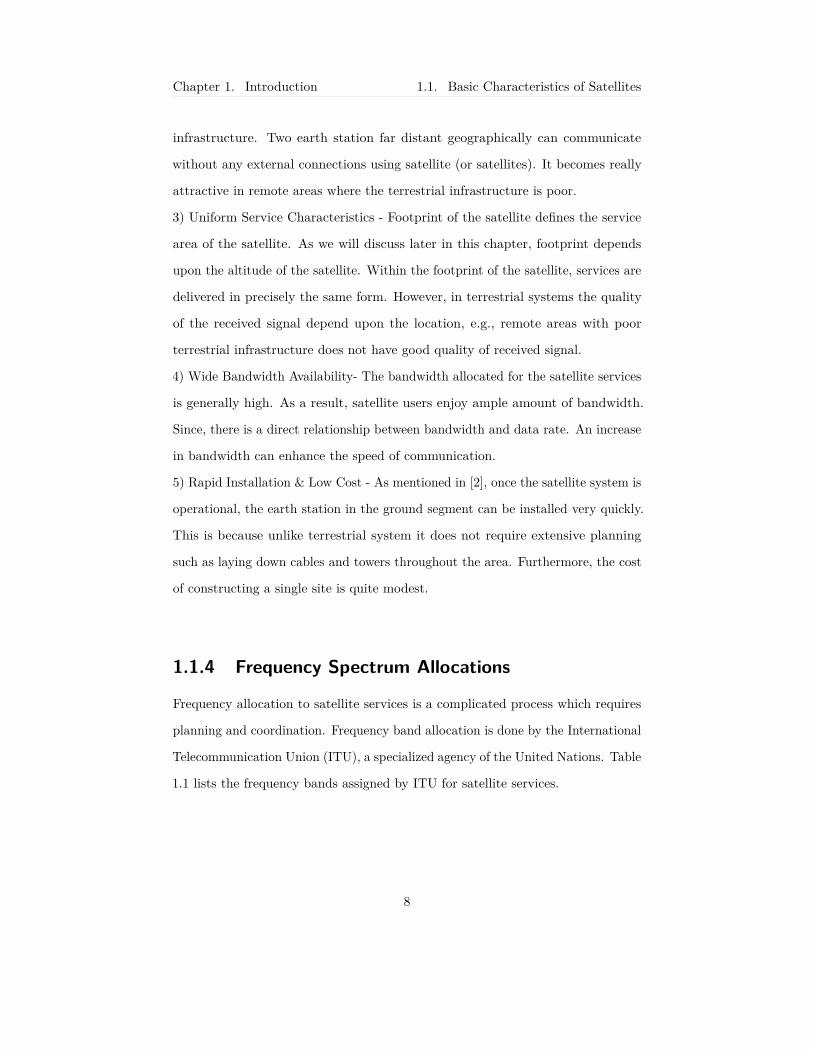
In the same way we will repeat the calculations when the temperature outside the

satellite is 123∘C (396 K). In upper bound analysis we will consider the transmit

power to be 1 mW and the carrier frequency to be 1 THz.

Table 4.2 indicates the parameters considered in the lower bound analysis.

Table 4.2: Parameters - Upper bound

Figure 4.4: Gain required for SNR of 10 dB vs Distance (Upper Bound)

48

Fe = 1 THz, Pt= 1 mW, Tsys = 712.4 K 0.3 ~------------------------~

0.25

QJ 0.2 ~ i ~ ~ 0.15

-~ ro Q)

Ill 0.1

0.05 ------

--8=1 GHz ~ 8=5GHz - - 8=10GHz

-----o~-~--~-~--~-~--~-~--~--~-~

0 100 200 300 400 500 600 700 800 900 1000

Distance[km]

Fe = 1 THz, Pt= 1 mW, Tsys = 712.4 K

--8=1 GHz 0.9 ~ 8=5GHz

0.8

"f 0.7 6 .; ., 0.6 E ro ~ 05 ro Q)

Ill 0.4

0.3

0.2

- - 8=10 GHz

0.1 ~-~-~--~-~--~-~-~--~-~---' 0 100 200 300 400 500 600 700 800 900 1000

Distance[km]

Chapter 4. Link Budget Analysis 4.2. Antenna Gain Required - Upper Bound

Figure 4.5: Beamwidth vs Distance (Upper Bound)

Figure 4.6: Beam diameter vs Distance (Upper Bound)

The efective noise temperature in the upper bound analysis is 712.4 K. On

49

Chapter 4. Link Budget Analysis 4.3. Terahertz ISL vs Optical ISL

comparing the corresponding fgures in the lower bound and upper bound analysis,

we can say that there is a diference of about 10 dB in the gain of the antenna

required to achieve an SNR of 10 dB. It is also important to note that the

beamwidth is as low as 0.05 degrees in the upper bound analysis. This will lead to

the increase in the pointing requirements between transmitter and receiver.

4.3 Terahertz ISL vs Optical ISL

In this section, we will do a comparative analysis between the THz based ISL and

optical/laser based ISL. This comparison will be done on the basis of pointing

requirements in both the cases.

From [21], the beam diameter of a gaussian laser beam at a position z is given

by √ ( )2�

�(�) = 2�0 1 + , (4.4)��

where ��0

2

�� = , (4.5)�

and z is the axial distance, and �0 is the waist size. Waist size is the radius of the

laser beam at its narrowest point.

In our analysis, we will consider a red laser with wavelength of 650 nm.We

will assume the waist size to be 1 cm.This value is deliberately taken to be large

in order to show the big diference in the beam diameter of THz based ISL and

optical/laser based ISL. We will calculate the beam diameter for the same range

of distances, i.e., 50 km to 1000 km.

50

0.045

E o.04 6 .; a3 .~ 0.035

~ ~

CO 0.03

0.025

0.02 L--=--~--~-~--~-~-~--~-~---' 0 100 200 300 400 500 600 700 800 900 1000

Distance[km]


Figure 4.7: Beam diameter in Optical ISL

From Figure 4.7, we can see that the beam diameter is very less in the case

of optical/laser based ISL. Also, from Figure 4.8 the beam diameter in lower

bound analysis and upper bound analysis at 10 GHz is much higher than the

beam diameter in optical/laser based ISL. As a result, pointing requirements in

the case of optical/laser based ISL will be very high in comparison to THz based

ISL. We will need a highly accurate ATP subsystem in order to communicate with

the receiver. Thus, we can say that the efciency of THz based ISL is more in

comparison to optical based ISL.

51

0.5 ~------------------------~

0

I ;;; a3 -0.5 E .!!!

~ ro .., -1 ~ en ..9

-1 .5

--THz l ov.oer bound - - THz Upper bound -G- Laser

/' /

,,,,. ,,,,. --

--- ------- -------

-2 ~-~--~-~--~-~--~-~--~--~-~ 0 100 200 300 400 500 600 700 800 900 1000

Distance[km]


Figure 4.8: Optical ISL vs THz ISL

In this chapter, we devised link budget analysis and calculated the gain of the

transmitter and receiver antenna required to achieve an SNR of 10 dB. In the

worst case scenario of maximum distance between satellites (1000 km), maximum

noise temperature of 712.4 K, transmit power of 1 mW, carrier frequency of 1 THz

and bandwidth of 10 GHz, we have found the gain required to be 76 dB. This

high gain of the antenna can be achieved by using an array or refector antenna.

A mechanically scanned confocal ellipsoidal refector antenna system was reported

in [22]. The simulation results show to achieve a gain of 75 dB at 0.67 THz.

52

CHAPTER 5

Additional Challenges in THz based ISL

In this chapter we will look at some of the additional challenges that needs to be

addressed in THz based ISL. We will begin by looking at the possibility of multi

path propagation due to the presence of debris in the space and its impact on the

quality of communication. We will also consider the impact of the high relative

motion between the satellites.

5.1 Space Debris

Space debris is the collection of non-functional human made objects in the earth

orbit such as old satellites, fragments from disintegration, erosion and collisions.

As of July 2013, more than 170 million debris smaller than 1 cm, about 670,000

debris 1-10 cm, and around 29000 larger debris were estimated to be in orbit.

Most of these debris are present in LEO and MEO [23]. In our analysis,we are

making use of THz radiation which means a wavelength of around 10−4 m. From

Sec.2.4, we can say that the scattering which will occur due to the space debris

will be geometric scattering. We need to take into account the refections which

53

Chapter 5. Additional Challenges in THz based ISL 5.1. Space Debris

will occur due to the space debris which can lead to multi path propagation.

In the next section, we will develop a simulation model for the multi path

propagation due to space debris in THz based ISL.

5.1.1 System Model

To model the number of multipath components, we need to take into account

propagation loss, the geometry of the network and the density of space debris.

LOS & NLOS propagation loss

Using equation (2.5), we can say that the total path loss for the line-of-sight (LOS)

component can be given by

( )24�� (�, �) = , (5.1)

�

where f is the operating frequency in Hz, d is the separation between the transmitter

and receiver, c is the speed of light in free space.

For the components which are not in line-of-sight (NLOS),we need to account

for the refection loss which occurs when the signal collides with an obstacle. In

this case, the total path loss can be given by

( )24�� (�, �) = �(�), (5.2)

�

where �(� ) is the refection coefcient.

Network Topology

The origin of the coordinate system is assumed to be at the mid-point of the distance

between two satellites. The transmitting and receiving satellites are placed at

equal distance d/2 from the origin on the x axis. We consider directional antennas

54


�2

�

� � ��

(−�/2, 0) �1

(�/2, 0)

Figure 5.1: Geometry of the Network considered. Refection occuring at point A.

are deployed at both the transmitter and receiver with �� as the beamwidth. We

also consider that diferent obstacles are randomly distributed in the space by

following a spatial Poisson process with rate �. Since poisson process is a stationary

independent increment process, the probability of fnding k objects in the area A

is given by (��)�

�−�� (�∈�) = . (5.3)�!

As shown in Figure 5.1, due to an obstacle (space junk) at point A there is

refection of the signal. As a result, another copy of the same transmitted signal is

received at ��. In our analysis, we have considered only single bounce refections.

5.1.2 Simulation Model

In this section we will perform simulations to fnd out the number of multipaths

due to space debris in THz based ISL with respect to time. We chose the frequency

55

1 x 104

0.8

0.6 + + 0.4 +

E 0.2 ij. +

.r u C 0 + ++ ro cii + + 0 -02 + + +

-0.4 + + + -0.6

-0.8

-1 -5 -4 -3 -2 -1 0 1 2 3 4 5

Distance[m] x 105


at which we are transmitting to be 0.34 THz. The value of of beamwidth is

considered to be 0.5 degree. The distance between the satellites is considered to be

1000 km. Also, the value of refection coefcient is considered to be 1. The fnal

result was found by taking 1000 realizations of the system. The simulation result

is calculated by plotting the histogram of the number of multipaths with time.

In our analysis we have considered the density of the space debris to be 10-9 per

�2. We can see from the Figure 5.2 all the space debris that are enclosed in the

receive and transmit beam. These space debris will lead to multipath propagation.

Figure 5.2: Space debris enclosed in Transmit & Receive Beam,� = 10-9 per �2

56

4

3.5

,,, 3 .c ro _g. 2.5 "3 E 0 2 0 z

1.5

0.5

o~-~-~-~--~-~-~-~~-~-~-~ 3.3333 3.33332 3.33334 3.33336 3.33338 3.3334

Delay[ms]


Figure 5.3: Multipath components as function of path delay, � = 10-9 per �2

From Figure 5.3, we can see that as time increases the number of multipath

decreases. We can observe that the frst path arrives at the receiver at time 3.33

ms. This is because we have considered distance between transmitter and receiver

to be 1000 kilometer and the speed of light is 3 × 108 m/s. This plot is drawn

by calculating the total distance traversed by the signal from the transmitter to

the receiver via the refector. This total distance is divided by the speed of light

to calculate the time at which signal will arrive at the receiver. After that a

histogram is plotted for all the multipaths. This experiment is conducted 1000

times to calculate the average number of multipaths with time.

The model that we have developed in this chapter is very general which means

that it is independent of the technology used in PHY layer. This model can also

be extended to terrestrial environment with directional antennas. However, the

model that we have described above will change in the case of a bounded area

application.

57


From Figure 5.3, we can also see that the delay spread is about 0.1 ��. As

mentioned in Chapter 2, a high delay spread can lead to Intersymbol Interference

(ISI). ISI happens when the duration of the signal that we are transmitting is less

than the delay spread. In our scenario, since the bandwidth is in the order of GHz,

the duration of the signal will be of the order of nanoseconds. As a result, there

are chances of ISI in THz based ISL. So we need to take into account the impact

of space debris on the quality of the link.

5.1.3 Power Delay profle

In this section, we will develop a power delay profle for THz based ISL in presence

of space debris. In order to fnd the power delay profle we need to know the

probability that any multipath component does not get blocked in the way while

reaching at the receiver. We will consider the obstacles to be of circular shape with

radius r and they follow the same Poisson distribution as mentioned in Sec.5.1.1.

As described in [18], the probability that the signal does not get blocked in the

way while reaching at the receiver is given by

2)�� (�) = �−�(��+�� , (5.4)

where r is the radius of the object and d is the distance traveled by the multipath

component from the transmitter to the receiver. The power delay profle can now

be readily found by � �� (�, �� )

� �� (� ) = (5.5)�(�)�� (� = �� )

.

In our analysis,we have assumed the radius of the obstacles to be 5 cm and the

carrier frequency is taken to be 0.34 THz.

58

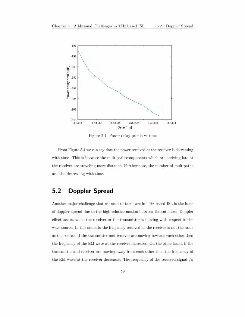
-198

cii'-200 ~ Q)

0: e -202 0. >,

"' -.; -o -204 t,:;

~ a. -206

-208

-210 ~-~-~--~-~--~-~-~--~-~-~ 3.3333 3.33332 3.33334 3.33336 3.33338 3.3334

Delay[ms]

Chapter 5. Additional Challenges in THz based ISL 5.2. Doppler Spread

Figure 5.4: Power delay profle vs time

From Figure 5.4 we can say that the power received at the receiver is decreasing

with time. This is because the multipath components which are arriving late at

the receiver are traveling more distance. Furthermore, the number of multipaths

are also decreasing with time.

5.2 Doppler Spread

Another major challenge that we need to take care in THz based ISL is the issue

of doppler spread due to the high relative motion between the satellites. Doppler

efect occurs when the receiver or the transmitter is moving with respect to the

wave source. In this scenario the frequency received at the receiver is not the same

as the source. If the transmitter and receiver are moving towards each other then

the frequency of the EM wave at the receiver increases. On the other hand, if the

transmitter and receiver are moving away from each other then the frequency of

the EM wave at the receiver decreases. The frequency of the received signal ��

59


can be given by

�� = �� − ��, (5.6)

where �� is the transmitter frequency and �� is the doppler frequency [24]. The

doppler frequency is given by �

�� = , (5.7)�

where v is the relative speed in the moving direction and � is the wavelength of

the EM wave.

In our analysis, the impact of the doppler spread can be very signifcant.

This is because the relative speed at which the satellites move can get very high.

Furthermore,we are transmitting at very low wavelength of about 30 �� to 3000

��. This high speed of the motion between the transmitter and receiver leads

to change in the impulse response of the channel. If the time within which the

channel changes is more than the duration of the signal then channel is considered

to be slow fading channel. On the other hand, if the channel response changing

time is less than the duration of the signal then the channel changes during the

transmission of the signal and there is distortion at the receiver. This channel is

considered to be fast fading channel.

In order to fnd the maximum duration of the signal that can be transmitted

without distortion at the receiver, we defne a measure called coherence time.

Coherence time is the statistical measure of the time duration over which the

channel impulse response is considered to be not varying [24].

Coherence time is related to the doppler frequency and is approximately given

by 9

�� = , (5.8)16��

where �� is the doppler frequency.

As calculated in [25], the maximum relative speed between satellites can go

60


as high as 8 km/sec. In our analysis we are making use of �� = 0.34� ��. Using

equation (5.7), we can calculate the doppler frequency to be 9 MHz. We can use

this value to calculate the coherence time. The value of the coherence time is

around 0.02 ��. Thus, if we want to transmit a signal without distortion at the

receiver the duration of the symbol should be less than 0.02 ��.In our analysis,

we used the transmission bandwidth to be 1 GHz, 5 GHz and 10 GHz. Since the

duration of the signal has an inverse relationship with the bandwidth, the duration

in our case would be of the order of nanoseconds. As a result, we will not be facing

the issue of fast fading at the receiver. However, we still need to compensate for

the doppler spread at the receiver.

61

CHAPTER 6

Conclusions and Future Work

In this research, we studied the feasibility of THz band for Inter-satellite communi-

cation. We developed the propagation model and analyzed the factors which can

afect THz wave propagation in ISL. We also studied about the noise sources which

can impact the quality of the signal. In order to maintain a specifed quality of the

link, we calculated the gain of the antenna required at the transmitter and receiver

in the worst case scenario. Based upon the pointing requirements, a comparative

analysis between laser based ISL and THz based ISL was also conducted and it

was shown that the latter has more efciency. Lastly, we analyzed the impact of

space debris leading to multipath propagation and doppler spread on THz based

ISL.

As part of future work, we need to design the modulation techniques to be

used for implementing THz based ISL. Also, the value of beamwidth required

to maintain the quality of the link is low, as a result, an accurate tracking and

pointing subsystem needs to be implemented on the satellites. Furthermore, we

need to properly choose high gain antennas considering the budget on the size of

the payload.

62

Bibliography

[1] Bruce Elbert. Introduction to Satellite Communication. Artech House,2008.

[2] Dennis Roddy. Satellite Communications. 2nd edition,McGraw Hill,1990.

[3] S. U. Hwu and K. B. deSilva and C. T. Jih. Terahertz (THz) wireless systems for space applications. IEEE Sensors Applications Symposium Proceedings,2013.

[4] S. W. Dong and Z. b. Zhu and Y. Wang Advances of terahertz research and terahertz satellite communications. International Conference on Electronics, Communications and Control (ICECC),2011.

[5] W. Dou and L. Zhang and H. Meng and Z. Wang Tracking antennas for inter-satellite communications at sub-millimeter wavelengths. 3rd Asia-Pacifc Conference on Antennas and Propagation,2014.

[6] R. Radhakrishnan, W. W. Edmonson, F. Afghah, R. M. Rodriguez-Osorio, F. Pinto and S. C. Burleigh Survey of Inter-Satellite Communication for Small Satellite Systems. IEEE Communications Surveys & Tutorials, vol. 18, no. 4, pp. 2442-2473, Fourthquarter 2016.

[7] Sun, R and Maessen, D and Guo, Jian and Gill, Eberhard Enabling inter-satellite communication and ranging for small satellites. 2017.

[8] J. Y. Suen, M. T. Fang, S. P. Denny and P. M. Lubin Modeling of Terabit Geostationary Terahertz Satellite Links From Globally Dry Locations. IEEE Journal of Selected Topics in Quantum Electronics, vol. 16, no. 5, pp. 1051-1057, Sept.-Oct. 2010.

[9] Z. Sodnik, B. Furch and H. Lutz, Optical Intersatellite Communication. IEEE Transactions on Terahertz Science and Technology, vol. 5, no. 2, pp. 299-313, March 2015.

[10] M. Guelman, A. Kogan, A. Kazarian, A. Livne, M. Orenstein and H. Michalik, Optical Intersatellite Communication. IEEE Transactions on Aerospace and Electronic Systems, vol. 40, no. 4, pp. 1239-1248, Oct. 2004.

[11] Zell, Holly Earth’s Atmospheric Layers. NASA, 2 Mar 2015.

63

Bibliography Bibliography

[12] H.Kaushal and G.kaddoum Optical Communication in Space: Challenges and Mitigation Techniques. IEEE Communications Surveys & Tutorials, vol. 19, no. 1, pp. 57-96, Firstquarter 2017.

[13] Rayleigh scattering. Wikipedia(2018, April 26).

[14] R. N. Mahalati and J. M. Kahn, Efect of fog on free-space optical links employing imaging receivers Opt. Exp., vol. 20, no. 2, pp. 1649–661, 2012.

[15] J. M. Wallace and P. V. Hobbs Atmospheric Science: An Introductory. Acad-emic Press, 1977.

[16] H. Willebrand and B. S. Ghuman Free Space Optics: Enabling Optical Con-nectivity in Today’s Networks. Sams Publishing, 2002

[17] P.F Panter Communications System Design. McGraw Hill,New York, 1972

[18] Z.Hossain,C.Mollica and J.M.Jornet Stochastic Multipath Channel Model-ing and Power Delay Profle Analysis for Terahertz-band Communication. Nanocom,2017.

[19] T. Nagatsuma, H. Song, and Y. Kado Challenges for ultrahighspeed wireless communications using Terahertz waves. Terahertz Sci. Technol., vol. 3, no. 2, pp. 55-65, Jun. 2010

[20] C.A Balanis Antenna Theory: Analysis and Design. 3rd edition,Wiley,2005

[21] D.G Aviv Laser Space Communications. Arctech House,2006

[22] N. Llombart, K. B. Cooper, R. J. Dengler, T. Bryllert and P. H. Siegel Confocal Ellipsoidal Refector System for a Mechanically Scanned Active Terahertz Imager. IEEE Transactions on Antennas and Propagation, vol. 58, no. 6, pp. 1834-1841, June 2010.

[23] Garcia, Mark. Space Debris and Human Spacecraft.NASA NASA, 14 Apr. 2015.

[24] E.bernal Mor Principles of cellular communication network 2016.

[25] M. T. Fatehi, H. Valencia, M. R. Davenport, A. Pandya, M. Trinca and V. Mehta A Study of the Relative Speed and Doppler Efects in Space-Based Networks 2008 IEEE Aerospace Conference, Big Sky, MT, 2008, pp. 1-11.

[26] Y. Matsumoto, M. Tanaka, S.Kozono, and T. Takahashi Evaluation of System Noise Temperature of S-Band Intersatellite Communications Equipment on ETS-VI satellite equipment Electronics and Communications in Japan, Part 1, Vol.80, No.1,1997

[27] I. F. Akyildiz, J. M. Jornet and M. Pierobon Propagation Models for Nanocom-munication Networks Proc. of the 4th European Conference on Antennas and Propagation (EuCAP),Barcelona, Spain, April 2010

64

Bibliography Bibliography

[28] Thuraya SatSleeve+ Satellite Phone for IPhone & Android | Outftter Satellite Phones. Outftter Satellite Inc.

[29] Space Segment.GPS.gov Agricultural Applications.

[30] Catalog of Earth Satellite Orbits : Feature Articles NASA.

[31] R/spacex - Iridium NEXT Constellation Mission 5 Launch Campaign Thread. Reddit

[32] Dunbar, Brian. "Tracking and Data Relay Satellite (TDRS)." NASA. NASA, 28 Apr. 2015

[33] JAXA | Optical Inter-orbit Communications Engineering Test Satellite "KI-RARI" (OICETS) Japan Aerospace Exploration Agency

[34] Atmospheric Absorption & Transmission.Electromagnetic Spectrum. HSU

[35] Satellite Coverage.Introduction to Radar Systems Dept of ECE, The University of Choice

65

https://Segment.GPS.gov

TERAHERTZ COMMUNICATION FOR SATELLITE NETWORKS

Documents

Transcript of TERAHERTZ COMMUNICATION FOR SATELLITE NETWORKS