TeraData Material

TCS Confidential

Teradata Parallel Architecture

Table of Contents

Table of Contents..............................................................................2

Chapter 1: Teradata Parallel Architecture..........................................11

Teradata Introduction..............................................................................11

Teradata Architecture..............................................................................12Teradata Components...........................................................................................................13

A Teradata Database...............................................................................16CREATE / MODIFY DATABASE Parameters.............................................................................16

Teradata Users........................................................................................17{ CREATE | MODIFY } DATABASE or USER (in common)........................................................17{ CREATE | MODIFY } USER (only).........................................................................................17

Symbols Used in this Book.......................................................................17

DATABASE Command...............................................................................18

Use of an Index.......................................................................................18Primary Index........................................................................................................................20Secondary Index....................................................................................................................21

Determining the Release of Your Teradata System:...................................22

Chapter 2: Fundamental SQL Using Select.........................................23

Fundamental Structured Query Language (SQL)........................................23

Basic SELECT Command...........................................................................24

WHERE Clause.........................................................................................26

Compound Comparisons (AND / OR)..........................................................27

Impact of NULL on Compound Comparisons..............................................30

Using NOT in SQL Comparisons................................................................31

Multiple Value Search (IN).......................................................................35Using NOT IN.........................................................................................................................36

Using Quantifiers Versus IN.....................................................................37

Multiple Value Range Search (BETWEEN)..................................................38

Character String Search (LIKE).................................................................39

Derived Columns.....................................................................................42

Creating a Column Alias Name.................................................................46AS.......................................................................................................................................... 46NAMED..................................................................................................................................47Naming conventions..............................................................................................................48Breaking Conventions...........................................................................................................49

ORDER BY...............................................................................................49

TCS Confidential

TOP Rows Option.....................................................................................52

DISTINCT Function...................................................................................53

Chapter 3: Online-HELP and SHOW commands...................................55

SHOW commands....................................................................................65

EXPLAIN..................................................................................................68

Adding Comments...................................................................................72ANSI Comment......................................................................................................................72Teradata Comment...............................................................................................................72

User Information Functions......................................................................73ACCOUNT Function................................................................................................................73DATABASE Function..............................................................................................................73SESSION Function..................................................................................................................74

Chapter 4: Data Conversions............................................................75

Data Conversions....................................................................................75

Data Types..............................................................................................75

CAST.......................................................................................................78

Implied CAST...........................................................................................79

Formatted Data.......................................................................................80Tricking the ODBC to Allow Formatted Data..........................................................................83

TITLE Attribute for Data Columns.............................................................83

Transaction Modes..................................................................................84

Case Sensitivity of Data...........................................................................85

CASESPECIFIC.........................................................................................86

LOWER Function......................................................................................87

UPPER Function.......................................................................................87

Chapter 5: Aggregation....................................................................89

Aggregate Processing..............................................................................89Math Aggregates...................................................................................................................89The SUM Function..................................................................................................................89The AVG Function..................................................................................................................89The MIN Function...................................................................................................................89The MAX Function..................................................................................................................89The COUNT Function.............................................................................................................90Aggregates and Derived Data...............................................................................................91

GROUP BY...............................................................................................92

Limiting Output Values Using HAVING......................................................95

Statistical Aggregates.............................................................................96The KURTOSIS Function.........................................................................................................97The SKEW Function...............................................................................................................98The STDDEV_POP Function....................................................................................................98

TCS Confidential

The STDDEV_SAMP Function.................................................................................................99The VAR_POP Function........................................................................................................100The VAR_SAMP Function......................................................................................................100The CORR Function..............................................................................................................101The COVAR Function...........................................................................................................102The REGR_INTERCEPT Function...........................................................................................103The REGR_SLOPE Function..................................................................................................104Using GROUP BY..................................................................................................................105Use of HAVING.....................................................................................................................105

Using the DISTINCT Function with Aggregates........................................106

Aggregates and Very Large Data Bases (VLDB).......................................106Potential of Execution Error.................................................................................................107GROUP BY versus DISTINCT.................................................................................................107

Performance Opportunities....................................................................109

Chapter 6: Subquery Processing.....................................................110

Subquery..............................................................................................110Using NOT IN.......................................................................................................................114Using Quantifiers.................................................................................................................114

Qualifying Table Names and Creating a Table Alias..................................116Qualifying Column Names...................................................................................................116Creating an Alias for a Table...............................................................................................117

Correlated Subquery Processing.............................................................117

EXISTS..................................................................................................119

Chapter 7: Join Processing..............................................................121

Join Processing......................................................................................121

Original Join Syntax...............................................................................122

Product Join..........................................................................................126

Newer ANSI Join Syntax.........................................................................129INNER JOIN..........................................................................................................................129OUTER JOIN.........................................................................................................................132LEFT OUTER JOIN.................................................................................................................133RIGHT OUTER JOIN...............................................................................................................135FULL OUTER JOIN.................................................................................................................137CROSS JOIN.........................................................................................................................140Self Join...............................................................................................................................142Alternative JOIN / ON Coding...............................................................................................143

Adding Residual Conditions to a Join.......................................................144INNER JOIN..........................................................................................................................144OUTER JOIN.........................................................................................................................145

OUTER JOIN Hints..................................................................................148

Parallel Join Processing..........................................................................149

Join Index Processing.............................................................................150

Chapter 8: Date and Time Processing..............................................151

TCS Confidential

DATE, TIME, and TIMESTAMP..................................................................151

ANSI Standard DATE Reference..............................................................152

INTEGERDATE........................................................................................152

ANSIDATE.............................................................................................153

DATEFORM............................................................................................153System Level Definition.......................................................................................................153User Level Definition...........................................................................................................153Session Level Declaration....................................................................................................154

DATE Processing....................................................................................154

ADD_MONTHS........................................................................................157

ANSI TIME.............................................................................................158

EXTRACT...............................................................................................159

Implied Extract of Day, Month and Year..................................................161

ANSI TIMESTAMP...................................................................................162

TIME ZONES..........................................................................................162Setting TIME ZONES............................................................................................................163Using TIME ZONES...............................................................................................................163Normalizing TIME ZONES.....................................................................................................165

DATE and TIME Intervals........................................................................166Using Intervals....................................................................................................................167INTERVAL Arithmetic with DATE and TIME...........................................................................167CAST Using Intervals...........................................................................................................169

OVERLAPS.............................................................................................170

System Calendar...................................................................................171

Chapter 9: Character String Processing...........................................176

Transforming Character Data.................................................................176

CHARACTERS Function...........................................................................177

CHARACTER_LENGTH Function................................................................179

OCTET_LENGTH Function........................................................................180

TRIM.....................................................................................................182

SUBSTRING...........................................................................................183

SUBSTR.................................................................................................185

SUBSTRING and Numeric Data................................................................186

POSITION..............................................................................................187

INDEX...................................................................................................188

SUBSTRING and POSITION or INDEX Used Together.................................189

Concatenation of Character Strings........................................................189

TCS Confidential

Chapter 10: OLAP Functions...........................................................194

On-Line Analytical Processing (OLAP) Functions......................................194

OLAP Functions.....................................................................................196

Cumulative Sum Using the CSUM Function..............................................196Cumulative Sum with Reset Capabilities.............................................................................200Generating Sequential Numbers with CSUM........................................................................202

Moving Sum Using the MSUM Function...................................................203Moving Sum with Reset Capabilities....................................................................................206

Moving Average Using the MAVG Function..............................................208Moving Average with Reset Capabilities..............................................................................210

Moving Difference Using the MDIFF Function..........................................212Moving Difference with Reset Capabilities...........................................................................214

Cumulative and Moving SUM Using SUM / OVER......................................216Cumulative Sum with Reset Capabilities.............................................................................220

Moving Average Using AVG / OVER.........................................................223Moving Average with Reset Capabilities..............................................................................225

Moving Linear Regression Using the MLINREG Function...........................226

Partitioning Data Using the QUANTILE Function......................................228QUALIFY to Find Products in the top Partitions....................................................................230

Ranking Data using RANK......................................................................234QUALIFY to Find Top Best or Bottom Worse.........................................................................236RANK with Reset Capabilities..............................................................................................238

Internal RANK operations.......................................................................239

Sampling Rows using the SAMPLE Function............................................239

RANDOM Number Generator Function.....................................................243

Chapter 11: SET Operators.............................................................244

Set Operators........................................................................................244

Considerations for Using Set Operators..................................................245

INTERSECT............................................................................................245

UNION...................................................................................................248

EXCEPT.................................................................................................251

MINUS...................................................................................................252

Using Multiple Set Operators in a Single Request....................................252

Chapter 12: Data Manipulation.......................................................255

Data Maintenance.................................................................................255Considerations for Data Maintenance..................................................................................255Safeguards..........................................................................................................................255

INSERT Command..................................................................................256

TCS Confidential

Using Null for DEFAULT VALUES..........................................................................................257

INSERT / SELECT Command....................................................................258Fast Path INSERT / SELECT..................................................................................................259

UPDATE Command.................................................................................260Fast Path UPDATE................................................................................................................262

DELETE Command..................................................................................263Fast Path DELETE................................................................................................................265

UPSERT.................................................................................................267

ANSI Vs Teradata Transactions...............................................................268

Performance Issues With Data Maintenance............................................268Impact of FALLBACK on Row Modification...........................................................................269Impact of PERMANENT JOURNAL Logging on Row Modification............................................269Impact of Primary Index on Row Modification......................................................................270Impact of Secondary Indices on Row Modification...............................................................270

Chapter 13: Data Interrogation.......................................................271

Data Interrogation.................................................................................271

NULLIFZERO..........................................................................................271

NULLIF..................................................................................................274

ZEROIFNULL..........................................................................................276

COALESCE.............................................................................................278

CASE.....................................................................................................280Flexible Comparisons within CASE.......................................................................................282Comparison Operators within CASE.....................................................................................284CASE for Horizontal Reporting.............................................................................................285Nested CASE Expressions....................................................................................................286CASE used with the other DML............................................................................................288

Using CASE to avoid a join.....................................................................289

Chapter 14: View Processing...........................................................290

Views....................................................................................................290Reasons to Use Views..........................................................................................................290Considerations for Creating Views.......................................................................................290

Creating and Using VIEWS......................................................................291

Deleting Views......................................................................................295

Modifying Views....................................................................................295

Modifying Rows Using Views..................................................................296DML Restrictions when using Views.....................................................................................296INSERT using Views.............................................................................................................296UPDATE or DELETE using Views..........................................................................................297WITH CHECK OPTION...........................................................................................................297

Locking and Views.................................................................................298

TCS Confidential

CREATE MACRO.....................................................................................300

REPLACE MACRO...................................................................................301

DROP MACRO........................................................................................304

Generating SQL from a Macro.................................................................304

Chapter 16: Transaction Processing................................................305

What is a Transaction............................................................................305

Locking.................................................................................................306

Transaction Modes................................................................................308

Comparison Chart..................................................................................309

ANSI Mode Transactions........................................................................312

Aborting Teradata Transactions.............................................................313

Aborting ANSI Transactions....................................................................314

Chapter 17: Reporting Totals and Subtotals.....................................315

Totals and Subtotals..............................................................................315

Totals (WITH)........................................................................................316

Subtotals (WITH…BY).............................................................................318Multiple Subtotals on a Single Break...................................................................................320Multiple Subtotal Breaks......................................................................................................321

Chapter 18: Data Definition Language.............................................324

Creating Tables.....................................................................................324

Table Considerations.............................................................................324Maximum Columns per Table..............................................................................................325

CREATE TABLE.......................................................................................325Column Data Types.............................................................................................................327Specifying the Database in a CREATE TABLE Statement.....................................................328

PRIMARY INDEX considerations..............................................................329Table Type Specifications of SET VS MULTISET...................................................................330SET and MULTISET Tables...................................................................................................330

Protection Features...............................................................................331FALLBACK............................................................................................................................332Permanent Journal...............................................................................................................333BEFORE Journal...................................................................................................................333AFTER Journal......................................................................................................................333

Internal Storage Options........................................................................334DATABLOCKSIZE..................................................................................................................335FREESPACE PERCENTAGE....................................................................................................335

Column Attributes.................................................................................336

Constraints...........................................................................................338UNIQUE Constraint..............................................................................................................339

TCS Confidential

CHECK Constraint................................................................................................................339Referential Integrity (RI) Constraint.....................................................................................340Defining Constraints at the Column level............................................................................340Defining Constraints at the Table Level...............................................................................341

Utilizing Default Values for a Table.........................................................341

CREATE TABLE to Copy an existing table.................................................342

Altering a Table.....................................................................................343

Dropping a Table...................................................................................345Dropping a Table versus Deleting Rows..............................................................................345

Renaming a Table..................................................................................345

Using Secondary Indices........................................................................346

Join Index..............................................................................................348

Hashing Functions.................................................................................351HASHROW...........................................................................................................................351HASHBUCKET......................................................................................................................352HASHAMP............................................................................................................................353HASHBAKAMP......................................................................................................................355

Conclusion............................................................................................357

Chapter 19: Temporary Tables........................................................357

Temporary Tables..................................................................................357Creating Interim or Temporal Tables...................................................................................358

Temporary Table Choices.......................................................................362

Derived Tables......................................................................................362

Volatile Temporary Tables......................................................................366

Global Temporary Tables.......................................................................369GLOBAL Temporary Table Examples...................................................................................370

General Practices for Temporary use Tables............................................373

Chapter 20: Trigger Processing.......................................................374

Triggers................................................................................................374Terminology........................................................................................................................374Logic Flow...........................................................................................................................375

CREATE TRIGGER Syntax........................................................................376Row Trigger.........................................................................................................................376Statement Trigger...............................................................................................................377‘BEFORE’ Trigger.................................................................................................................378‘AFTER’ Trigger....................................................................................................................379‘INSTEAD OF’ Trigger...........................................................................................................379

Cascading Triggers................................................................................380

Sequencing Triggers..............................................................................383

Chapter 21: Stored Procedures.......................................................383

TCS Confidential

Teradata Stored Procedures...................................................................383

CREATE PROCEDURE..............................................................................385

Stored Procedural Language (SPL) Statements.......................................385BEGIN / END Statements.....................................................................................................386

Establishing Variables and Data Values..................................................388DECLARE Statement to Define Variables.............................................................................388SET to Assign a Data Value as a Variable............................................................................389Status Variables..................................................................................................................390Assigning a Data Value as a Parameter...............................................................................390

Additional SPL Statements.....................................................................391CALL Statement...................................................................................................................391IF / END IF Statement..........................................................................................................392LOOP / END LOOP Statements.............................................................................................394LEAVE Statement................................................................................................................394WHILE / END WHILE Statement...........................................................................................395FOR / END FOR Statements.................................................................................................396ITERATE Statement.............................................................................................................398PRINT Statement.................................................................................................................399

Exception Handling................................................................................399DECLARE HANDLER Statement............................................................................................399

DML Statements....................................................................................400

Using Column and Alias Names...............................................................401

Comments and Stored Procedures..........................................................402Commenting in a Stored Procedure.....................................................................................402Commenting on a Stored Procedure....................................................................................402

On-line HELP for Stored Procedures........................................................403HELP on a Stored Procedure................................................................................................403HELP on Stored Procedure Language (SPL).........................................................................405

REPLACE PROCEDURE............................................................................406

DROP PROCEDURE.................................................................................406

RENAME PROCEDURE.............................................................................406

SHOW PROCEDURE................................................................................406

Other New V2R4.1 Features...................................................................407

Considerations When Using Stored Procedures.......................................407

Compiling a Procedure...........................................................................407Temporary Directory Usage................................................................................................408

TCS Confidential

Chapter 1: Teradata Parallel Architecture

Teradata Introduction

TCS Confidential

The world's largest data warehouses commonly use the superior technology of NCR's Teradata relational database management system (RDBMS). A data warehouse is normally loaded directly from operational data. The majority, if not all of this data will be collected on-line as a result of normal business operations. The data warehouse therefore acts as a central repository of the data that reflects the effectiveness of the methodologies used in running a business.

As a result, the data loaded into the warehouse is mostly historic in nature. To get a true representation of the business, normally this data is not changed once it is loaded. Instead, it is interrogated repeatedly to transform data into useful information, to discover trends and the effectiveness of operational procedures. This interrogation is based on business rules to determine such aspects as profitability, return on investment and evaluation of risk.

For example, an airline might load all of its maintenance activity on every aircraft into the database. Subsequent investigation of the data could indicate the frequency at which certain parts tend to fail. Further analysis might show that the parts are failing more often on certain models of aircraft. The first benefit of the new found knowledge regards the ability to plan for the next failure and maybe even the type of airplane on which the part will fail. Therefore, the part can be on hand when and maybe where it is needed or the part might be proactively changed prior to its failure.

If the information reveals that the part is failing more frequently on a particular model of aircraft, this could be an indication that the aircraft manufacturer has a problem with the design or production of that aircraft. Another possible cause is that the maintenance crew is doing something incorrectly and contributing to the situation. Either way, you cannot fix a problem if you do not know that a problem exists. There is incredible power and savings in this type of knowledge.

Another business area where the Teradata database excels is in retail. It provides an environment that can store billions of sales. This is a critical capability when you are recording and analyzing the sales of every item in every store around the world. Whether it is used for inventory control, marketing research or credit analysis, the data provides an insight into the business. This type of knowledge is not easily attainable without detailed data that records every aspect of the business. Tracking inventory turns, stock replenishment, or predicting the number of goods needed in a particular store yields a priceless perspective into the operation of a retail outlet. This information is what enables one retailer to thrive while others go out of business.

Teradata is flourishing with the realization that detail data is critical to the survival of a business in a competitive, lower margin environment. Continually, businesses are forced to do more with less. Therefore, it is vital to maximize the efforts that work well to improve profit and minimize or correct those that do not work.

One computer vendor used these same techniques to determine that it cost more to sell into the desktop environment than was realized in profit. Prior to this realization, the sales effort had attempted to make up the loss by selling more computers. Unfortunately, increased sales meant increased losses. Today, that company is doing much better and has made a huge step into profitability by discontinuing the small computer line.

Teradata Architecture

The Teradata database currently runs normally on NCR Corporation's WorldMark Systems in the UNIX MP-RAS environment. Some of these systems consist of a single processing node (computer) while others are several hundred nodes working together in a single system. The NCR nodes are based entirely on industry standard CPU processor chips, standard internal and external bus architectures like PCI and SCSI, and standard memory modules with 4-way interleaving for speed.

TCS Confidential

At the same time, Teradata can run on any hardware server in the single node environment when the system runs Microsoft NT and Windows 2000. This single node may be any computer from a large server to a laptop.

Whether the system consists of a single node or is a massively parallel system with hundreds of nodes, the Teradata RDBMS uses the exact same components executing on all the nodes in parallel. The only difference between small and large systems is the number of processing components.

When these components exist on different nodes, it is essential that the components communicate with each other at high speed. To facilitate the communications, the multi-node systems use the BYNET as the interconnect between the nodes. It is a high speed, multi-path, dual redundant communications channel. Another amazing capability of the BYNET is that the bandwidth increases with each consecutive node added into the system. There is more detail on the BYNET later in this chapter.

Teradata Components

As previously mentioned, Teradata is the superior product today because of its parallel operations based on its architectural design. It is the parallel processing by the major components that provide the power to move mountains of data. Teradata works more like the early Egyptians who built the pyramids without heavy equipment using parallel, coordinated human efforts. It uses smaller nodes running several processing components all working together on the same user request. Therefore, a monumental task is completed in record time.

Teradata operates with three major components to achieve the parallel operations. These components are called: Parsing Engine Processors, Access Module Processors and the Message Passing Layer. The role of each component is discussed in the next sections to provide a better understanding of Teradata. Once we understand how Teradata works, we will pursue the SQL that allows storage and access of the data.

Parsing Engine Processor (PEP or PE)

The Parsing Engine Processor (PEP) or Parsing Engine (PE), for short, is one of the two primary types of processing tasks used by Teradata. It provides the entry point into the database for users on mainframe and networked computer systems. It is the primary director task within Teradata.

As users "logon" to the database they establish a Teradata session. Each PE can manage 120 concurrent user sessions. Within each of these sessions users submit SQL as a request for the database server to take an action on their behalf. The PE will then parse the SQL statement to establish which database objects are involved. For now, let's assume that the database object is a table. A table is a two-dimensional array that consists of rows and columns. A row represents an entity stored in a table and it is defined using columns. An example of a row might be the sale of an item and its columns include the UPC, a description and the quantity sold.

Any action a user requests must also go through a security check to validate their privileges as defined by the database administrator. Once their authorization at the object level is verified, the PE will verify that the columns requested actually exist within the objects referenced.

Next, the PE optimizes the SQL to create an execution plan that is as efficient as possible based on the amount of data in each table, the indices defined, the type of indices, the selectivity level of the indices, and the number of processing steps needed to retrieve the data. The PE is responsible for passing the optimized execution plan to other components as the best way to gather the data.

An execution plan might use the primary index column assigned to the table, a secondary index or a full table scan. The use of an index is preferable and will be discussed later in this chapter. For now, it is

TCS Confidential

sufficient to say that a full table scan means that all rows in the table must be read and compared to locate the requested data.

Although a full table scan sounds really bad, within the architecture of Teradata, it is not necessarily a bad thing because the data is divided up and distributed to multiple, parallel components throughout the database. We will look next at the AMPs that perform the parallel disk access using their file system logic. The AMPs manage all data storage on disks. The PE has no disks.

Activities of a PE: Convert incoming requests from EBCDIC to ASCII (if from an IBM mainframe) Parse the SQL to determine type and validity Validate user privileges Optimize the access path(s) to retrieve the rows Build an execution plan with necessary steps for row access Send the plan steps to Access Module Processors (AMP) involved

Access Module Processor (AMP)

The next major component of Teradata's parallel architecture is called an Access Module Processor (AMP). It stores and retrieves the distributed data in parallel. Ideally, the data rows of each table are distributed evenly across all the AMPs. The AMPs read and write data and are the workhorses of the database. Their job is to receive the optimized plan steps, built by the PE after it completes the optimization, and execute them. The AMPs are designed to work in parallel to complete the request in the shortest possible time.

Optimally, every AMP should contain a subset of all the rows loaded into every table. By dividing up the data, it automatically divides up the work of retrieving the data. Remember, all work comes as a result of a users' SQL request. If the SQL asks for a specific row, that row exists in its entirety (all columns) on a single AMP and other rows exist on the other AMPs.

If the user request asks for all of the rows in a table, every AMP should participate along with all the other AMPs to complete the retrieval of all rows. This type of processing is called an all AMP operation and an all rows scan. However, each AMP is only responsible for its rows, not the rows that belong to a different AMP. As far as the AMPs are concerned, it owns all of the rows. Within Teradata, the AMP environment is a "shared nothing" configuration. The AMPs cannot access each other's data rows, and there is no need for them to do so.

Once the rows have been selected, the last step is to return them to the client program that initiated the SQL request. Since the rows are scattered across multiple AMPs, they must be consolidated before reaching the client. This consolidation process is accomplished as a part of the transmission to the client so that a final comprehensive sort of all the rows is never performed. Instead, all AMPs sort only their rows (at the same time — in parallel) and the Message Passing Layer is used to merge the rows as they are transmitted from all the AMPs.

Therefore, when a client wishes to sequence the rows of an answer set, this technique causes the sort of all the rows to be done in parallel. Each AMP sorts only its subset of the rows at the same time all the other AMPs sort their rows. Once all of the individual sorts are complete, the BYNET merges the sorted rows. Pretty brilliant!

Activities of the AMP: Store and retrieve data rows using the file system Aggregate data Join processing between multiple tables Convert ASCII returned data to EBCDIC (IBM mainframes only)

TCS Confidential

Sort and format output data

Message Passing Layer (BYNET)

The Message Passing Layer varies depending on the specific hardware on which the Teradata database is executing. In the latter part of the 20th century, most Teradata database systems executed under the UNIX operating system. However, in 1998, Teradata was released on Microsoft's NT operating system. Today it also executes under Windows 2000. The initial release of Teradata, on the Microsoft systems, is for a single node.

When using the UNIX operating system, Teradata supports up to 512 nodes. This massively parallel system establishes the basis for storing and retrieving data from the largest commercial databases in the world, Teradata. Today, the largest system in the world consists of 176 nodes. There is much room for growth as the databases begin to exceed 40 or 50 terabytes.

For the NCR UNIX systems, the Message Passing Layer is called the BYNET. The amazing thing about the BYNET is its capacity. Instead of a fixed bandwidth that is shared among multiple nodes, the bandwidth of the BYNET increases as the number of nodes increase. This feat is accomplished as a result of using virtual circuits instead of using a single fixed cable or a twisted pair configuration.

To understand the workings of the BYNET, think of a telephone switch used by local and long distance carriers. As more and more people place phone calls, no one needs to speak slower. As one switch becomes saturated, another switch is automatically used. When your phone call is routed through a different switch, you do not need to speak slower. If a natural or other type of disaster occurs and a switch is destroyed, all subsequent calls are routed through other switches. The BYNET is designed to work like a telephone switching network.

An additional aspect of the BYNET is that it is really two connection paths, like having two phone lines for a business. The redundancy allows for two different aspects of its performance. The first aspect is speed. Each path of the BYNET provides bandwidth of 10 Megabytes (MB) per second with Version 1 and 60 MB per second with Version 2. Therefore the aggregate speed of the two connections is 20MB/second or 120MB/second. However, as mentioned earlier, the bandwidth grows linearly as more nodes are added.

Using Version 1 any two nodes communicate at 40MB/second (10MB/second * 2 BYNETs * 2 nodes). Therefore, 10 nodes can utilize 200MB/second and 100 nodes have 2000MB/second available between them. When using the version 2 BYNET, the same 100 nodes communicate at 12,000MB/second (60MB/second * 2 BYNETs * 100 nodes).

The second and equally important aspect of the BYNET uses the two connections for availability. Regardless of the speed associated with each BYNET connection, if one of the connections should fail, the second is completely independent and can continue to function at its individual speed without the other connection. Therefore, communications continue to pass between all nodes.

Although the BYNET is performing at half the capacity during an outage, it is still operational and SQL is able to complete without failing. In reality, when the BYNET is performing at only 10MB/second per node, it is still a lot faster than many normal networks that typically transfer messages at 10MB per second.

All messages going across the BYNET offer guaranteed delivery. So, any messages not successfully delivered because of a failure on one connection automatically route across the other connection. Since half of the BYNET is not working, the bandwidth reduces by half. However, when the failed connection is returned to service, its topology is automatically configured back into service and it begins transferring messages along with the other connection. Once this occurs, the capacity returns to normal.

TCS Confidential

A Teradata Database

Within Teradata, a database is a storage location for database objects (tables, views, macros, and triggers). An administrator can use Data Definition Language (DDL) to establish a database by using a CREATE DATABASE command.

A database may have PERMANENT (PERM) space allocated to it. This PERM space establishes the maximum amount of disk space for storing user data rows in any table located in the database. However, if no tables are stored within a database, it is not required to have PERM space. Although a database without PERM space cannot store tables, it can store views and macros because they are physically stored in the Data Dictionary (DD) PERM space and require no user storage space. The DD is in a "database" called DBC.

Teradata allocates PERM space to tables, up to the maximum, as rows are inserted. The space is not pre-allocated. Instead, it is allocated, as rows are stored in blocks on disk. The maximum block size is defined either at a system level in the DBS Control Record, at the database level or individually for each table. Like PERM, the block size is a maximum size. Yet, it is only a maximum for blocks that contain multiple rows. By nature, the blocks are variable in length. So, disk space is not pre-allocated; instead, it is allocated on an as needed basis, one sector (512 bytes) at a time. Therefore, the largest possible wasted disk space in a block is 511 bytes.

A database can also have SPOOL space associated with it. All users who run queries need workspace at some point in time. This SPOOL space is workspace used for the temporary storage of rows during the execution of user SQL statements. Like PERM space, SPOOL is defined as a maximum amount that can be used within a database or by a user. Since PERM is not pre-allocated, unused PERM space is automatically available for use as SPOOL. This maximizes the disk space throughout the system.

It is a common practice in Teradata to have some databases with PERM space that contain only tables. Then, other databases contain only views. These view databases require no PERM space and are the only databases that users have privileges to access. The views in these databases control all access to the real tables in other databases. They insulate the actual tables from user access. There will be more on views later in this book.

The newest type of space allocation within Teradata is TEMPORARY (TEMP) space. A database may or may not have TEMP space, however, it is required if Global Temporary Tables are used. The use of temporary tables is also covered in more detail later in the SQL portion of this book.

A database is defined using a series of parameter values at creation time. The majority of the parameters can easily be changed after a database has been created using the MODIFY DATABASE command. However, when attempting to increase PERM or TEMP space maximums, there must be sufficient disk space available even though it is not immediately allocated. There may not be more PERM space defined that actual disk on the system.A number of additional database parameters are listed below along with the user parameters in the next section. These parameters are tools for the database administrator and other experienced users when establishing databases for tables and views.

CREATE / MODIFY DATABASE Parameters PERMANENT TEMPORARY SPOOL ACCOUNT FALLBACK JOURNAL DEFAULT JOURNAL

TCS Confidential

http://www.books24x7.com/viewer.asp?bkid=16589&destid=33#33


Teradata Users

In Teradata, a user is the same as a database with one exception. A user is able to logon to the system and a database cannot. Therefore, to authenticate the user, a password must be established. The password is normally established at the same time that the CREATE USER statement is executed. The password can also be changed using a MODIFY USER command.

Like a database, a user area can contain database objects (tables, views, macros and triggers). A user can have PERM and TEMP space and can also have spool space. On the other hand, a user might not have any of these types of space, exactly the same as a database.

The biggest difference between a database and a user is that a user must have a password. This similarity between the two makes administering the system easier and allows for default values that all databases and users can inherit.

The next two lists regard the creation and modification of databases and users.

{ CREATE | MODIFY } DATABASE or USER (in common) PERMANENT TEMPORARY SPOOL ACCOUNT FALLBACK JOURNAL DEFAULT JOURNAL

{ CREATE | MODIFY } USER (only) PASSWORD STARTUP DEFAULT DATABASE

By no means are these all of the parameters. It is not the intent of this chapter, nor the intent of this book to teach database administration. There are reference manuals and courses available to use. Teradata administration warrants a book by itself.

Symbols Used in this Book

Since there are no standard symbols for teaching SQL, it is necessary to understand some of the symbols used in our syntax diagrams throughout this book.

This chart should be used as a reference for SQL syntax used in the book:

Open table as spreadsheet This chart should be used as a reference for SQL syntax used in the book:

<database-name>

Substitute an actual database name in this location

<table-name> Substitute an actual table name in this location

TCS Confidential

Open table as spreadsheet This chart should be used as a reference for SQL syntax used in the book:

<comparison> Substitute a comparison in this location, i.e. a=1

<column-name> Substitute an actual column name in this location

<data-value> Substitute a literal data value in this location

[ optional entry ] Everything between the [ ] is optional, not required to be valid syntax , use when needed

{ use this | or this }

Use one of the keywords or symbols on either side of the "|", but not both. I.e. { LEFT | RIGHT } use either "LEFT" or "RIGHT" but not both and the left { and the right } are never used in SQL.

Figure 1-1

DATABASE Command

When users negotiate a successful logon to Teradata, they are automatically positioned in a default database as defined by the database administrator. When an SQL request is executed, by default, it looks in the current database for all referenced objects.

There may be times when the object is not in the current database. When this happens, the user has one of two choices to resolve this situation. One solution is to qualify the name of the object along with the name of the database in which it resides. To do this, the user simply associates the database name to the object name by connecting them with a period (.) or dot as shown below:

<database-name>.<table-name>

The second solution is to use the database command. It repositions the user to the specified database. After the database command is executed, there is no longer a need to qualify the objects in that database. Of course, if the SQL statement references additional objects in another database, they will have to be qualified in order for the system to locate them. Normally, you will DATABASE to the database that contains most of the objects that you need. Therefore it reduces the number of object names requiring qualification.

The following is the syntax for the DATABASE command.

DATABASE <database-name> ;

If you are not sure what database you are in, either the HELP SESSION or SELECT DATABASE command may be used to make that determination. These commands and other HELP functions are covered in the SQL portion of this book.

Use of an Index

Although a relational data model uses Primary Keys and Foreign Keys to establish the relationships between tables, that design is a Logical Model. Each vendor uses specialized techniques to implement a Physical Model. Teradata does not use keys in its physical model. Instead, Teradata is implemented using indices, both primary and secondary.

TCS Confidential

http://www.books24x7.com/book/id_16589/outputobject.asp?bookid=16589&chunkid=549645810&objectid=nr-N27&objecttype=spreadsheet

The Primary Index (PI) is the most important index in all of Teradata. The performance of Teradata can be linked directly to the selection of this index. The data value in the PI column(s) is submitted to the hashing function. The resulting row hash value is used to map the row to a specific AMP for data distribution and storage.

To illustrate this concept, I have on several occasions used two decks of cards. Imagine if you will, fourteen people in a room. To the largest, most powerful looking man in the room, you give one of the decks of cards. His large hands allow him to hold all fifty-two cards at one time, with some degree of success. The cards are arranged with the ace of spades continuing through the king of spades in ascending order. After the spades, the hearts come next, then the clubs and last, the diamonds. Each suit is arranged starting with the ace and ascending up to the king. The cards are partitioned by suit.

The other deck of cards is divided among the other thirteen people. Using this procedure, all cards with the same value (i.e. aces) all go to the same person. Likewise, all the deuces, treys and subsequent cards each go to one of the thirteen people. Each of the four cards will be in the same order as the suits contained in the single deck that went to the lone man: spades, hearts, clubs and diamonds. Once all the cards have been distributed, each of the thirteen people will be holding four cards of the same value (4*13=52). Now, the game can begin.

The requests in this game come in the form of "give-me," one or more cards.

To make it easy for the lone player, we first request: give-me the ace of spades. The person with four aces finds their ace, as does the lone player with all 52 cards, both on the top other their cards. That was easy!

As the difficulty of the give-me requests increase, the level of difficulty dramatically increases for the lone person. For instance, when a give-me request is for all of the twos, only one of the thirteen people holds up all four of their cards and it is finished. The lone man must locate the 2 of spades between the ace and trey. Then, go and locate the 2 of hearts, thirteen cards later between the ace and trey. Then, find the 2 of clubs, thirteen cards after that, as well as the 2 of diamonds, and thirteen cards after that to finally complete the request.

Another request might be give-me all of the diamonds. For the thirteen people, each person locates and holds up one card of their cards and the request is finished. For the lone person with the single deck, the request means finding and holding up the last thirteen cards in their deck of fifty-two. In each of these give-me requests, the lone man had to negotiate all fifty two cards while the thirteen other people only needed to determine which of the four cards applied to the request, if any. This is the same procedure used by Teradata. It divides up the data like we divided up the cards.

As illustrated, the thirteen people are faster than the lone man. However, the game is not limited to thirteen players. If there were 26 people who wished to play on the same team, the cards simply need to be divided or distributed differently.

When using the value (ace through king) there are only 13 unique values. In order for 26 people to play, we need a way to come up with 26 unique values for 26 people. To make the cards more unique, we might combine the value of the card (i.e. ace) with the color. Therefore, we have two red aces and two black aces as well as two sets for every other card. Now when we distribute the cards, each of the twenty-six people receives only two cards instead of the original four. The distribution is still based on fifty-two cards (2 times 26).

At the same time, the optimum number of people for the game is not 26. Based on what has been discussed so far, what is the optimum number of people?

If your answer is 52, then you are absolutely correct.

TCS Confidential

With this many people, each person has one and only one card. Any time a give-me is requested of the participants, their one card either qualifies or it does not. It doesn't get any simpler or faster than this situation.

As easy as this may sound, to accomplish this distribution the value of the card alone is not sufficient to manifest 52 unique values. Neither is using the value and the color. That combination only gives us a distribution of 26 unique values when 52 unique values are desired.

To achieve this distribution we need to establish still more uniqueness. Fortunately, we can use the suit along with the value. Therefore, the ace of spades is different than the ace of hearts, which is different from the ace of clubs and the ace of diamonds. In other words, there are now 52 unique identities to use for distribution.

To relate this distribution to Teradata, one or more columns of a table are chosen to be the Primary Index.

Primary Index

The Primary Index can consist of up to 16 different columns prior to V2R6 and 64 columns with that release. These columns, when considered together, provide a comprehensive technique to derive a Unique Primary Index (UPI, pronounced as "you-pea") value as we discussed previously regarding the card analogy. That is the good news.

To store the data, the value(s) in the PI are hashed via a calculation to determine which AMP will own the data. The same data values always hash the same row hash and therefore are always associated with the same AMP.

The advantage to using up to sixteen columns is that row distribution is very smooth or evenly based on unique values. This simply means that each AMP contains the same number of rows. At the same time, there is a downside to using several columns for a PI. The PE needs every data value for each column as input to the hashing calculation to directly access a particular row. If a single column value is missing, a full table scan will result because the row hash cannot be recreated. Any row retrieval using the PI column(s) is always an efficient, one AMP operation.

Although uniqueness is good in most cases, Teradata does not require that a UPI be used. It also allows for a Non-Unique Primary Index (NUPI, pronounced as new-pea). The potential downside of a NUPI is that if several duplicate values (NUPI dups) are stored, they all go to the same AMP. This can cause an uneven distribution that places more rows on some of the AMPs than on others. This means that any time an AMP with a larger number of rows is involved, it has to work harder than the other AMPs. The other AMPs will finish before the slower AMP. The time to process a single user request is always based on the slowest AMP. Therefore, serious consideration should be used when making the decision to use a NUPI.

Every table must have a PI and it is established when the table is created. If the CREATE TABLE statement contains: UNIQUE PRIMARY INDEX (<column-list>), the value in the column(s) will be distributed to an AMP as a UPI. However, if the statement reads: PRIMARY INDEX (<column-list>), the value in the column(s) will be distributed as a NUPI and allow duplicate values. Again, all the same values will go to the same AMP.

If the DDL statement does not specify a PI, but it specifies a PRIMARY KEY (PK), the named column(s) are used as the UPI. Although Teradata does not use primary keys, the DDL may be ported from another vendor's database system.

A UPI is used because a primary key must be unique and cannot be null. By default, both UPIs and NUPIs allow a null value to be stored unless the column definition indicates that null values are not allowed using a NOT NULL constraint.

TCS Confidential

Now, with that being said, when considering JOIN accesses on the tables, sometimes it is advantageous to use a NUPI. This is because the rows being joined between tables must be on the same AMP. If they are not on the same AMP, one of the rows must be moved to the same AMP as the matching row. Teradata will use one of two different strategies to temporarily move rows. It can copy all needed rows to all AMPs or it can redistribute them using the hashing mechanism on the column defined as the join domain that is a PI. However, if neither join column is a PI, it might be necessary to redistribute all participating rows from both tables by hash code to get them together on a single AMP.

Planning data distribution, using access characteristics, can reduce the amount of data movement and therefore improve join performance. This works fine as long as there are a consistent number of duplicate values or only a small number of duplicate values. The logical data model needs to be extended with usage information in order to know the best way to distribute the data rows. This is done during the physical implementation phase before creating tables.

Secondary Index

A Secondary Index (SI) is used in Teradata as a way to directly access rows in the data, sometimes called the base table, without requiring the use of PI values. Unlike the PI, an SI does not effect the distribution of the data rows. Instead, it is an alternate read path and allows for a method to locate the PI value using the SI. Once the PI is obtained, the row can be directly accessed using the PI. Like the PI, an SI can consist of up to 16 columns until V2R6 and then up to 64 columns.

In order for an SI to retrieve the data row by way of the PI, it must store and retrieve an index row. To accomplish this Teradata creates, maintains and uses a subtable. The PI of the subtable is the value in the column(s) that are defined as the SI. The "data" stored in the subtable row is the previously hashed value of the real PI for the data row or rows in the base table. The SI is a pointer to the real data row desired by the request. An SI can also be unique (USI, pronounced as you-sea) or non-unique (NUSI, as new-sea).

The rows of the subtable contain the row hashed value of the SI, the actual data value(s) of the SI, and the row hashed value of the PI as the row ID. Once the row ID of the PI is obtained from the subtable row, using the hashed value of the SI, the last step is to get the actual data row from the AMP where it is stored. The action and hashing for an SI is exactly the same as when starting with a PI. When using a USI, the access of the subtable is a one AMP operation and then accessing the data row from the base table is another one AMP operation. Therefore, USI accesses are always a two AMP operation based on two separate row hash operations. When using a NUSI, the subtable access is always an all AMP operation. Since the data is distributed by the PI, NUSI duplicate values may exist and probably do exist on multiple AMPs. So, the best plan is to go to all AMPs and check for the requested NUSI value.

To make this more efficient, each AMP scans its subtable. These subtable rows contain the row hash of the NUSI, the value of the data that created the NUSI and one or more row IDs for all the PI rows on that AMP. This is still a fast operation because these rows are quite small and several are stored in a single block. If the AMP determines that it contains no rows for the value of the NUSI requested, it is finished with its portion of the request. However, if an AMP has one or more rows with the requested NUSI value, it then goes and retrieves the data rows into spool space using the index.

With this said, the SQL optimizer may decide that there are too many base table data rows to make index access efficient. When this happens, the AMPs will do a full base table scan to locate the data rows and ignore the NUSI. This situation is called a weakly selective NUSI. Even using old-fashioned indexed sequential files, it has always been more efficient to read the entire file and not use an index if more than 15% of the records were needed. This is compounded with Teradata because the "file" is read in parallel instead of all data from a single file. So, the efficiency percentage is probably closer to being less than 3%

TCS Confidential

of all the rows in order to use the NUSI. If the SQL does not use a NUSI, you should consider dropping it, due to the fact that the subtable takes up PERM space with no benefit to the users. The Teradata EXPLAIN is covered in this book and it is the easiest way to determine if your SQL is using a NUSI. Furthermore, the optimizer will never use a NUSI without STATISTICS.

There has been another evolution in the use of NUSI processing. It is called NUSI Bitmapping. This means that if a table has two different NUSI indices and individually they are weakly selective, but together they can be bitmapped together to eliminate most of the non-conforming rows; it will use the two different NUSI columns together because they become highly selective. Therefore, many times, it is better to use smaller individual NUSI indices instead of a large composite (more than one column) NUSI.

There is another feature related to NUSI processing that can improve access time when a value range comparison is requested. When using hash values, it is impossible to determine any value within the range. This is because large data values can generate small hash values and small data values can produce large hash values. So, to overcome the issue associated with a hashed value, there is a range feature called Value Ordered NUSIs. At this time, it may only be used with a four byte or smaller numeric data column. Based on its functionality, a Value Ordered NUSI is perfect for date processing. See the DDL chapter in this book for more details on USI and NUSI usage.

Determining the Release of Your Teradata System:SELECT * FROM DBC.DBCINFO;

InfoKey InfoData

RELEASE V2R.05.01.03.00

VERSION 05.01.03.00

TCS Confidential

Chapter 2: Fundamental SQL Using Select

Fundamental Structured Query Language (SQL)

The access language for all modern relational database systems (RDBMS) is Structured Query Language (SQL). It has evolved over time to be the standard. The ANSI SQL group defines which commands and functionality all vendors should provide within their RDBMS.

There are three levels of compliance within the standard: Entry, Intermediate and Full. The three level definitions are based on specific commands, data types and functionalities. So, it is not that a vendor has incorporated some percentage of the commands; it is more that each command is categorized as belonging to one of the three levels. For instance, most data types are Entry level compliant. Yet, there are some that fall into the Intermediate and Full definitions.

Since the standard continues to grow with more options being added, it is difficult to stay fully ANSI compliant. Additionally, all RDBMS vendors provide extra functionality and options that are not part of the standard. These extra functions are called extensions because they extend or offer a benefit beyond those in the standard definition.

At the writing of this book, Teradata was fully ANSI Entry level compliant based on the 1992 Standards document. NCR also provides much of the Intermediate and some of the Full capabilities. This book indicates feature by feature which SQL capabilities are ANSI and which are Teradata specific, or extensions. It is to NCR's benefit to be as compliant as possible in order to make it easier for customers of other RDBMS vendors to port their data warehouse to Teradata.

As indicated earlier, SQL is used to access, store, remove and modify data stored within a relational database, like Teradata. The SQL is actually comprised of three types of statements. They are: Data Definition Language (DDL), Data Control Language (DCL) and Data Manipulation Language (DML). The primary focus of this book is on DML and DDL. Both DDL and DCL are, for the most part, used for administering an RDBMS. Since the SELECT statement is used the vast majority of the time, we are concentrating on its functionality, variations and capabilities.

Everything in the first part of this chapter describes ANSI standard capabilities of the SELECT command. As the statements become more involved, each capability will be designated as either ANSI or a Teradata Extension.

TCS Confidential

Basic SELECT Command

Using the SELECT has been described like playing the game, Jeopardy. The answer is there; all you have to do is come up with the correct question.

The basic structure of the SELECT statement indicates which column values are desired and the tables that contain them. To aid in the learning of SQL, this book will capitalize the SQL keywords. However, when SQL is written for Teradata, the case of the statement is not important. The SQL statements can be written using all uppercase, lowercase or a combination; it does not matter to the Teradata PE.

The SELECT is used to return the data value(s) stored in the columns named within the SELECT command. The requested columns must be valid names defined in the table(s) listed in the FROM portion of the SELECT.The following shows the format of a basic SELECT statement. In this book, the syntax uses expressions like: <column-name> (see Figure 1-1) to represent the location of one or more names required to construct a valid SQL statement:

SEL[ECT] { <column-name> | * }

[…,<column-name]

FROM <table-name> ;

The structure of the above command places all keywords on the left in uppercase and the variable information such as column and table names to the right. Like using capital letters, this positioning is to aid in learning SQL. Lastly, although the use of SEL is acceptable in Teradata, with [ECT] in square brackets being optional, it is not ANSI standard.

Lastly, when multiple column names are requested in the SELECT, a comma must separate them. Without the separator, the optimizer cannot determine where one ends and the next begins.

The following syntax format is also acceptable:

SEL[ECT] <column-name> FROM <table-name> ;

Both of these SELECT statements produce the output report, but the above style is easier to read and debug for complex queries. The output display might appear as:

3 Rows Returned

<column-name>

aaaaaaaaaaaaaaaaaa

bbbbbbbbbbbbbbbb

cccccccccccccccccc

In the output, the column name becomes the default heading for the report. Then, the data contained in the selected column is displayed once for each row returned.

The next variation of the SELECT statement returns all of the columns defined in the table indicated in the FROM portion of the SELECT.

SEL[ECT] *

FROM <table-name> ;

The output of the above request uses each column name as the heading and the columns are displayed in the same sequence as they are defined in the table. Depending on the tool used to submit the request,

TCS Confidential


care should be taken, because if the returned display is wider than the media (i.e. terminal=80 and paper=133); it may be truncated.

At times, it is desirable to select the same column twice. This is permitted and to accomplish it, the column name is simply listed in the SELECT column list more than once. This technique might often be used when doing aggregations or calculating a value, both are covered in later chapters.

The table below is used to demonstrate the results of various requests. It is a small table with a total of ten rows for easy comparison.For Example: the next SELECT might be used with Figure 2-1, to display the student number, the last name, first name, the class code and grade point for all of the students in the Student table:

SELECT *

FROM Student_Table ;

Open table as spreadsheet Student Table - contains 10 students

Student_ID Last_Name First_name Class_code Grade_Pt

PK

FK

UPI NUSI

NUSI

123250 Phillips Martin SR 3.00

125634 Hanson Henry FR 2.88

234121 Thomas Wendy FR 4.00

231222 Wilson Susie SO 3.80

260000 Johnson Stanley

280023 McRoberts Richard JR 1.90

322133 Bond Jimmy JR 3.95

324652 Delaney Danny SR 3.35

333450 Smith Andy SO 2.00

423400 Larkins Michael FR 0.00

Figure 2-1

10 Rows returned

Student_ID Last_Name First_Name Class_Code Grade_Pt




260000 Johnson Stanley ? ?

TCS Confidential


http://www.books24x7.com/book/id_16589/viewer_r.asp?bookid=16589&chunkid=905243847#ch02fig01568563DA-4631-4281-B789-D756B9D3D1CB%23ch02fig01568563DA-4631-4281-B789-D756B9D3D1CB








Notice that Johnson has question marks in the grade point and class code columns. Most client software uses the question mark to represent missing data or an unknown value (NULL). More discussion on this condition will appear throughout this book. The other thing to note is that character data is aligned from left to right, the same as we read it and numeric is from right to left, from the decimal.

This SELECT returns all of the columns except the Student ID from the Student table:

SELECT First_name

,Last_name

,Class_Code

,Grade_Pt


10 Rows returned

First_Name Last_Name Class_Code Grade_Pt

Michael Larkins FR 0.00

Henry Hanson FR 2.88

Richard McRoberts JR 1.90

Stanley Johnson ? ?

Susie Wilson SO 3.80

Wendy Thomas FR 4.00

Danny Delaney SR 3.35

Martin Phillips SR 3.00

Jimmy Bond JR 3.95

Andy Smith SO 2.00

There is no short cut for selecting all columns except one or two. Also, notice that the columns are displayed in the output in the same sequence they are requested in the SELECT statement.

WHERE Clause

The previous "unconstrained" SELECT statement returned every row from the table. Since the Teradata database is most often used as a data warehouse, a table might contain millions of rows. So, it is wise to request only certain types of rows for return.

TCS Confidential

By adding a WHERE clause to the SELECT, a constraint is established to potentially limit which rows are returned based on a TRUE comparison to specific criteria or set of conditions.

SEL[ECT] * | <column-name> }

[…,<column-name> ]

FROM <table-name>

WHERE { <column-name> | <expression> } <comparison> <data-value> ;

Open table as spreadsheet The conditional check in the WHERE can use the ANSI comparison operators (symbols are ANSI / alphabetic are Teradata Extension):

Equal Not Equal

Less Than

Greater Than

Less Than or Equal

Greater Than or Equal

= <> < > <= >=

EQ NE LT GT LE GE

Figure 2-2

The following SELECT can be used to return the students with a B (3.0) average or better from the Student table:

SELECT Student_ID

,Last_Name

,Grade_Pt

FROM Student_Table

WHERE Grade_Pt >= 3.0 ;

5 Rows returned

Student_ID Last_Name Grade_Pt

231222 Wilson 3.80

234121 Thomas 4.00

324652 Delaney 3.35

123250 Phillips 3.00

322133 Bond 3.95

Without the WHERE clause, the AMPs return all of the rows in the table to the user. ore and more Teradata user systems are getting to the point where they are storing illions of rows in a single table. There must be a very good reason for needing to see all of them. More simply put, you will always use a WHERE clause whenever you want to see only a portion of the rows in a table.

Compound Comparisons (AND / OR)

Many times a single comparison is not sufficient to specify the desired rows. To add more functionality to the WHERE clause, it is common to use more than one comparison. The multiple condition checks and column names are not separated by a comma, like column names. Instead, they must be connected using a logical operator.

TCS Confidential


The following is the syntax for using the AND logical operator:

SEL[ECT] <column-name>


FROM <table-name>

WHERE <column-name> <comparison> <data-value> { AND | OR }

<column-name> <comparison> <data-value> ;

Notice that the column name is listed for each comparison separated by a logical operator; this will be true even when it is the same column being compared twice. The AND signifies that each individual comparison on both sides of the AND must be true. The final result of the comparison must be TRUE for a row to be returned.

Open table as spreadsheet This Truth Table illustrates this point using AND.

First Test Result AND Second Test Result Final Result

True True True

True False False

False True False

False False False

Figure 2-3

When using AND, different columns must be used because a single column can never contain more than a single data value.

Therefore, it does not make good sense to issue the next SELECT using an AND on the same column because no rows will ever be returned.

SELECT Last_Name

,First_Name

FROM Student_Table

WHERE Grade_Pt = 3.0 AND Grade_Pt = 4.0;

No rows found

The above SELECT will never return any rows. It is impossible for a column to contain more than one value. No student has a 3.0 grade average AND a 4.0 average. They might have one or the other, but not both. It might contain one or the other, but never both at the same time. The AND operator indicates both must be TRUE and should never be used between two comparisons on the same column.

By substituting an OR logical operator for the previous AND, rows will now be returned.

The following is the syntax for using OR:

SELECT Student_ID

,Last_Name

,First_Name

,Grade_Pt

FROM Student_Table

TCS Confidential


WHERE Grade_Pt = 3.0 OR Grade_Pt = 4.0 ;

2 Rows returned

Student_ID Last_Name First_Name Grade_Pt

234121 Thomas Wendy 4.00

123250 Phillips Martin 3.00

The OR signifies that only one of the comparisons on each side of the OR needs to be true for the entire test to result in a true and the row to be selected.

Open table as spreadsheet This Truth Table illustrates the results for the OR:

First Test Result OR Second Test Result Final Result

True True True

True False True

False True True

False False False

Figure 2-4

When using the OR, the same column or different column names may be used. In this case, it makes sense to use the same column because a row is returned when a column contains either of the specified values as opposed to both values as seen with AND.

It is perfectly legal and common practice to combine the AND with the OR in a single SELECT statement.

The next SELECT contains both an AND as well as an OR:

SELECT *

FROM Student_Table

WHERE Grade_Pt = 3.0 OR Grade_Pt = 4.0 AND Class_Code = 'FR' ;

2 Rows returned




At first glance, it appears that the comparison worked correctly. However, upon closer evaluation it is incorrect because Phillips is a senior and not a freshman.

When mixing AND with OR in the same WHERE clause, it is important to know that the AND is evaluated first. The previous SELECT actually returns all rows with a grade point of 3.0. Hence, Phillips was returned. The second comparison returned Thomas with a grade point of 4.0 and a class code of 'FR'.

When it is necessary for the OR to be evaluated before the AND the use of parentheses changes the priority of evaluation. A different result is seen when doing the OR first. Here is how the statement should be written:

SELECT Last_Name

TCS Confidential


,Class_Code

,Grade_Pt

FROM Student_Table

WHERE (Grade_Pt = 3.0 OR Grade_Pt = 4.0) AND Class_Code = 'FR' ;

1 Row returned

Last_Name Class_Code Grade_Pt

Thomas FR 4.00

Now, only Thomas is returned and the output is correct.

Impact of NULL on Compound Comparisons

NULL is an SQL reserved word. It represents missing or unknown data in a column. Since NULL is an unknown value, a normal comparison cannot be used to determine whether it is true or false. All comparisons of any value to a NULL result in an unknown; it is neither true nor false. The only valid test for a null uses the keyword NULL without the normal comparison symbols and is explained in this chapter.

When a table is created in Teradata, the default for a column is for it to allow a NULL value to be stored. So, unless the default is over-ridden and NULL values are not allowed, it is a good idea to understand how they work.A SHOW TABLE command (chapter 3) can be used to determine whether a NULL is allowed. If the column contains a NOT NULL constraint, you need not be concerned about the presence of a NULL because it is disallowed.

Open table as spreadsheet This AND Truth Table must now be used for compound tests when NULL values are allowed:

First Test Result AND Second Test Result Final Result

True Unknown Unknown

Unknown True Unknown

False Unknown False

Unknown False False

Unknown Unknown Unknown

Figure 2-5

Open table as spreadsheet This OR Truth Table must now be used for compound tests when NULL values are allowed:


True Unknown True

Unknown True True

False Unknown Unknown

TCS Confidential



Open table as spreadsheet This OR Truth Table must now be used for compound tests when NULL values are allowed:


Unknown False Unknown

Unknown Unknown Unknown

Figure 2-6

For most comparisons, an unknown (null) is functionally equivalent to a false because it is not a true. Therefore, when using any comparison symbol a row is not returned when it contains a NULL.

At the same time, the next SELECT does not return Johnson because all comparisons against a NULL are unknown:

SELECT *

FROM Student_Table

WHERE Grade_Pt = NULL AND Class_Code = NULL ;

No rows foundV2R5: *** Failure 3731 The user must use IS NULL or IS NOT NULL to test for NULL values.

As seen in the above Truth tables, a comparison test cannot be used to find a NULL.To find a NULL, it becomes necessary to make a slight change in the syntax of the conditional comparison. The coding necessary to find a NULL is seen in the next section.

Using NOT in SQL Comparisons

It can be fairly straightforward to request exactly which rows are needed. However, sometimes rows are needed that contain any value other than a specific value. When this is the case, it might be easier to write the SELECT to find what is not needed instead of what is needed. Then convert it to return everything else. This might be the situation when there are 100 potential values stored in the database table and 99 of them are needed. So, it is easier to eliminate the one value than it is to specifically list the desired 99 different values individually.

Either of the next two SELECT formats can be used to accomplish the elimination of the one value:


FROM <table-name>

WHERE <column-name> NOT <comparison> <data-value> ;

Or


FROM <table-name>

WHERE NOT (<column-name> <comparison> <data-value>) ;

This second version of the SELECT is normally used when compound conditions are required. This is because it is usually easier to code the SELECT to get what is not wanted and then to enclose the entire set of comparisons in parentheses and put one NOT in front of it. Otherwise, with a single comparison, it is easier to put NOT in front of the comparison operator without requiring the use of parentheses.

TCS Confidential



The next SELECT uses the NOT with an AND comparison to display seniors and lower classmen with grade points less than 3.0:

SELECT Last_Name

,First_Name

,Class_Code

,Grade_Pt

FROM Student_Table

WHERE NOT (Grade_Pt >= 3.0 AND Class_Code <> 'SR') ;

6 Rows returned

Last_Name First_Name Class_Code Grade_Pt

McRoberts Richard JR 1.90

Hanson Henry FR 2.88

Delaney Danny SR 3.35

Larkins Michael FR 0.00

Phillips Martin SR 3.00

Smith Andy SO 2.00

Without using the above technique of a single NOT, it is necessary to change every individual comparison. The following SELECT shows this approach, notice the other change necessary below, NOT AND is an OR:

Since you cannot have conditions like: NOT >= and NOT <>, they must be converted to < (not < and not =) and = (not, not =). It returns the same 5 rows, but also notice that the AND is now an OR:

SELECT Last_Name

,First_Name

,Class_Code

,Grade_Pt

FROM Student_Table

WHERE Grade_Pt < 3.0 OR Class_Code = 'SR' ;

6 Rows returned







Smith Andy SO 2.00

TCS Confidential




Open table as spreadsheet Chart of individual conditions and NOT:

Condition Opposite condition

NOT condition

>= < NOT >=

<> = NOT <>

AND OR OR

OR AND AND

Figure 2-7

To maintain the integrity of the statement, all portions of the WHERE must be changed, including AND, as well as OR. The following two SELECT statements illustrate the same concept when using an OR:

SELECT Last_Name

FROM Student_Table

WHERE NOT (Grade_Pt >= 3.0 OR Grade_Pt <= 2.0) ;

Or

SELECT Last_Name

FROM Student_Table

WHERE Grade_Pt < 3.0 AND Grade_Pt > 2.0 ;

1 Row returned

Last_Name

Hanson

In the earlier Truth table, the NULL value returned an unknown when checked with a comparison operator. When looking for specific conditions, an unknown was functionally equivalent to a false, but really it is an unknown.

These two Truth tables can be used together as a tool when mixing AND and OR together in the WHERE clause along with NOT.

Open table as spreadsheet This Truth Table helps to gauge returned rows when using NOT with AND:

First Test Result AND Second Test Result Result

NOT(True)=False NOT(Unknown)=Unknown False

NOT(Unknown)=Unknown NOT(True)=False False

NOT(False)=True NOT(Unknown)=Unknown Unknown

TCS Confidential


Open table as spreadsheet This Truth Table helps to gauge returned rows when using NOT with AND:

First Test Result AND Second Test Result Result

NOT(Unknown)=Unknown NOT(False)=True Unknown

NOT(Unknown)=Unknown NOT(Unknown)=Unknown Unknown

Figure 2-8

Open table as spreadsheet This Truth Table can be used to gauge returned rows when using NOT with OR:

First Test Result OR Second Test Result Result

NOT(True)=False NOT(Unknown)=Unknown Unknown

NOT(Unknown)=Unknown NOT(True)=False Unknown

NOT(False)=True NOT(Unknown)=Unknown True

NOT(Unknown)=Unknown NOT(False)=True True

NOT(Unknown)=Unknown NOT(Unknown)=Unknown Unknown

Figure 2-9

There is an issue associated with using NOT. When a NOT is done on a true condition, the result is a false. Likewise, the NOT of a false is a true. However, when a NOT is done with an unknown, the result is still an unknown. Whenever a NULL appears in the data for any of the columns being compared, the row will never be returned and the answer set will not be what is expected.

It takes some practice and consideration when using NOT. Another area where care must be taken is when allowing NULL values to be stored in one or both of the columns. As mentioned earlier, previous versions of Teradata had no concept of "unknown" and if a compare didn't result in a true, it was false. With the emphasis on ANSI compatibility the unknown was introduced.

If NULL values are allowed and there is potential for the NULL to impact the final outcome of compound tests, additional tests are required to eliminate them. One way to eliminate this concern is to never allow a NULL value in any columns. However, this may not be appropriate and it will require more storage space because a NULL can be compressed. Therefore, when a NULL is allowed, the SQL needs to check for a NULL.

Using the expression IS NOT NULL is the only technique when NULL is allowed in a column and the NOT is used with a single or a compound comparison written as:

SELECT Last_Name, First_Name

,Class_Code

,Grade_Pt

FROM Student_Table

WHERE NOT (Grade_Pt >= 3.0 AND Grade_Pt IS NOT NULL AND

Class_Code <> 'SR' AND Class_Code IS NOT NULL) ;

TCS Confidential



7 Rows returned




McRoberts Richard R 1.90

Johnson Stanley ? ?



Smith Andy SO 2.00

Notice that Johnson came back this time and did not appear previously because of the NULL values.

Later in this book, the COALESCE will be explored as another way to eliminate NULL values directly in the SQL instead of in the database.

Multiple Value Search (IN)

Previously, it was shown that adding a WHERE clause to the SELECT limited the returned rows to those that meet the criteria. The IN comparison is an alternative to using one or more OR comparisons on the same column in the WHERE clause of a SELECT statement and the IN comparison also makes it a bit easier to code:



FROM <table-name>

WHERE <column-name> IN (<value-list>) ;

The value list normally consists of multiple values separated by commas. When the value in the column being compared matches one of the values in the list, the row is returned.

The following is an example for the alternative method when any one of the conditions is enough to satisfy the request using IN:

SELECT Last_Name

,Class_Code

,Grade_Pt

FROM Student_Table

WHERE Grade_Pt IN (2.0, 3.0, 4.0) ;

3 Row returned


Phillips SR 3.00

Thomas FR 4.00

Smith SO 2.00

TCS Confidential

The use of multiple conditional checks as well as the IN can be used in the same SELECT request. Considerations include the use of AND for declaring that multiple conditions must all be true. Earlier, we saw the solution using a compound OR.

Using NOT IN

As seen earlier, sometimes the unwanted values are not known or it is easier to eliminate a few values than to specify all the values needed. When this is the case, it is a common practice to use the NOT IN as coded below.

The next statement eliminates the rows that match and return those that do not match:

SELECT Last_Name

,Grade_Pt

FROM Student_Table

WHERE Grade_Pt NOT IN (2.0, 3.0, 4.0) ;

6 Rows returned

Last_Name Grade_Pt

McRoberts 1.90

Hanson 2.88

Wilson 3.80

Delaney 3.35

Larkins 0.00

Bond 3.95

The following SELECT is a better way to make sure that all rows are returned when using a NOT IN:

SELECT Last_Name

,Class_Code

,Grade_Pt

FROM Student_Table

WHERE Grade_Pt NOT IN (2.0, 3.0, 4.0) OR Grade_Pt IS NULL ;

7 Rows returned


Larkins FR 0.00

Hanson FR 2.88

McRoberts JR 1.90

Johnson ? ?

Wilson SO 3.80

Delaney SR 3.35

Bond JR 3.95

TCS Confidential

Notice that Johnson came back in this list and not the previous request using the NOT IN.

You may be thinking that if the NULL reserved word is used within the IN list it will cover the situation. Unfortunately, you are forgetting that this comparison always returns an unknown. Therefore, the next request will NEVER return any rows:

SELECT Last_Name

,Class_Code

,Grade_Pt

FROM Student_Table

WHERE Grade_Pt NOT IN (2.0, 3.0, 4.0, NULL) ;

No Rows found

Making this mistake will cause no rows to ever be returned. This is because every time the column is compared against the value list the NULL is an unknown and the Truth table shows that the NOT of an unknown is always an unknown for all rows.If you are not sure about this, do an EXPLAIN (chapter 3) of the NOT IN and a subquery to see that the AMP step will actually be skipped when a NULL exists in the list. There are also extra AMP steps to compensate for this condition. It makes the SQL VERY inefficient.

Using Quantifiers Versus IN

There is another alternative to using the IN. Quantifiers can be used to allow for normal comparison operators without requiring compound conditional checks.

The following is equivalent to an IN:



FROM <table-name>

WHERE <column-name> = ANY (<value-list>)

;

This next request uses ANY instead of IN:

SELECT Last_Name

,Class_Code

,Grade_Pt

FROM Student_Table

WHERE Grade_Pt = ANY (2.0, 3.0, 4.0) ;

3 Row returned


Phillips SR 3.00

Thomas FR 4.00

Smith SO 2.00

TCS Confidential


Using a qualifier, the equivalent to a NOT IN is:



FROM <table-name>

WHERE <column-name> NOT = ALL (<value-list>) ;

Notice that like adding a NOT to the compound condition, all elements need to be changed here as well. To reverse the = ANY, it becomes NOT = ALL. This is important, because the NOT = ANY selects all the rows except those containing a NULL. The reason is that as soon as a value is not equal to any one of the values in the list, it is returned.

The following SELECT is converted from an earlier NOT IN:

SELECT Last_Name

,Grade_Pt

FROM Student_Table

WHERE Grade_Pt NOT = ALL (2.0, 3.0, 4.0) ;

6 Rows returned

Last_Name Grade_Pt

McRoberts 1.90

Larkins 0.00

Hanson 2.88

Wilson 3.80

Delaney 3.35

Bond 3.95

Multiple Value Range Search (BETWEEN)

The BETWEEN comparison can be used as another technique to request multiple values for a column that are all in a specific range. It is easier than writing a compound OR comparison or a long value list of sequential numbers when using the IN.

This is a good time to point out that this chapter is incrementally adding new ways to compare for values within a WHERE clause. However, all of these techniques can be used together in a single WHERE clause. One method does not eliminate the ability to use one or more of the others using logical operators between each comparison.

The next SELECT shows the syntax format for using the BETWEEN:



FROM <table-name>

WHERE <column-name> BETWEEN <low-value> AND <high-value> ;

TCS Confidential

The first and second values specified are inclusive for the purposes of the search. In other words, when these values are found in the data, the rows are included in the output.

As an example, the following code returns all students whose grade points of 2.0, 4.0 and all values between them:

SELECT Grade_Pt

FROM Student_Table

WHERE Grade_Pt BETWEEN 2.0 and 4.0 ;

7 Rows returned

Grade_Pt

3.00

2.88

4.00

3.80

3.95

3.35

2.00

Notice that due to the inclusive nature of the BETWEEN, both 2.0 and 4.0 were included in the answer set. The first value of the BETWEEN must be the lower value, otherwise, no rows will be returned. This is because it looks for all values that are greater or equal to the first value and less than or equal to the second value.

A BETWEEN can also be used to search for character values. When doing this, care must be taken to insure that rows are received with the values that are needed. The system can only compare character values that are the same length. So, if one column or value is shorter than the other, the shortest will automatically be padded with spaces out to the same length as the longer value.Comparing 'CA' and 'CALIFORNIA' never constitutes a match. In reality, the database is comparing 'CA' with 'CALIFORNIA ' and they are not equal. Sometimes, it is easier to use the LIKE comparison operator which will be covered in the next section. Although, easier to code, it does not always mean faster to execute. There is always a trade-off to consider.

The next SELECT finds all of the students whose last name starts with an L:

SELECT Last_Name

FROM Student_Table

WHERE Last_Name BETWEEN 'L' AND 'LZ' ;

1 Row returned

Last_Name

Larkins

In reality, the WHERE could have used BETWEEN 'L' and 'M' as long as no student's last name was 'M'. The data needs to be understood when using BETWEEN for character comparisons.

Character String Search (LIKE)

TCS Confidential


The LIKE is used exclusively to search for character data strings. The major difference between the LIKE and the BETWEEN is that the BETWEEN looks for specific values within a range. The LIKE is normally used when looking for a string of characters within a column. Also, the LIKE has the capability to use "wildcard" characters.

Open table as spreadsheet The wildcard characters are:

Wildcard symbol

What it does

_ (underscore) matches any single character, but a character must be present

% (percent sign) matches any single character, a series of characters or the absence of characters

Figure 2-10

The next SELECT finds all rows that have a character string that begins with 'Sm':

SELECT *

FROM Student_Table

WHERE Last_Name LIKE 'sm%' ;

1 Row returned



The fact that the 's' is in the first position dictates its location in the data. Therefore, the 'm' must be in the second position. Then, the '%' indicates that any number of characters (including none) may be in the third and subsequent positions. So, if the WHERE clause contained: LIKE '%sm', it only looks for strings that end in "SM." On the other hand, if it were written as: LIKE '%sm%', then all character strings containing "sm" anywhere are returned.

Also, remember that in Teradata mode, the database is not case sensitive. However, in ANSI mode, the case of the letters must match exactly and the previous request must be written as 'Sm%' to obtain the same result. Care should be taken regarding case when working in ANSI mode. Otherwise, case does not matter.

The '_' wildcard can be used to force a search to a specific location in the character string. Anything in that position is considered a match but a character must be in there.

The following SELECT uses a LIKE to find all last names with an "A" in the second position of the last name:

SELECT *

FROM Student_Table

WHERE Last_Name LIKE ('_a%') ;

2 Rows returned




TCS Confidential


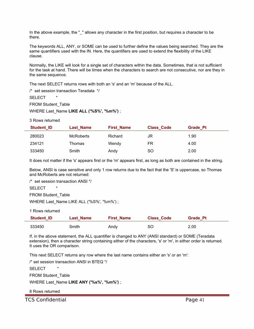
In the above example, the "_" allows any character in the first position, but requires a character to be there.

The keywords ALL, ANY, or SOME can be used to further define the values being searched. They are the same quantifiers used with the IN. Here, the quantifiers are used to extend the flexibility of the LIKE clause.

Normally, the LIKE will look for a single set of characters within the data. Sometimes, that is not sufficient for the task at hand. There will be times when the characters to search are not consecutive, nor are they in the same sequence.

The next SELECT returns rows with both an 's' and an 'm' because of the ALL.

/* set session transaction Teradata */

SELECT *

FROM Student_Table

WHERE Last_Name LIKE ALL ('%S%', '%m%') ;

3 Rows returned





It does not matter if the 's' appears first or the 'm' appears first, as long as both are contained in the string.

Below, ANSI is case sensitive and only 1 row returns due to the fact that the 'S' is uppercase, so Thomas and McRoberts are not returned:

/* set session transaction ANSI */

SELECT *

FROM Student_Table

WHERE Last_Name LIKE ALL ('%S%', '%m%') ;

1 Rows returned



If, in the above statement, the ALL quantifier is changed to ANY (ANSI standard) or SOME (Teradata extension), then a character string containing either of the characters, 's' or 'm', in either order is returned. It uses the OR comparison.

This next SELECT returns any row where the last name contains either an 's' or an 'm':

/* set session transaction ANSI in BTEQ */

SELECT *

FROM Student_Table

WHERE Last_Name LIKE ANY ('%s%', '%m%') ;

8 Rows returned

TCS Confidential





260000 Johnson Stanley ? ?





Always be aware of the issue regarding case sensitivity when using ANSI Mode. It will normally affect the number of rows returned and usually reduces the number of rows.

There is a specialty operation that can be performed in conjunction with the LIKE. Since the search uses the "_" and the "%" as wildcard characters, how can you search for actual data that contains a "_" or "%" in the data?

Now that we know how to use the wildcard characters, there is a way to take away the special meaning and literally make the wildcard characters an '_' and a '%'. That is the purpose of ESCAPE. It tells the PE to not match anything, but instead, match the actual character of '_' or '%'.

The next SELECT uses the ESCAPE to find all table names that have a "_" in the 8th position of the name from the Data Dictionary.

SELECT Tablename

FROM DBC.tables

WHERE Tablename LIKE ('_ _ _ _ _ _ _ \_%') ESCAPE '\'

AND Databasename = 'mikel' ;

2 Rows returnedTablename

Student_Table

Student_Course_Table

In the above output, the only thing that matters is the '_' in position eight because of the first seven '_' characters are still wildcards.

Derived Columns

The majority of the time, columns in the SELECT statement exist within a database table. However, sometimes it is more advantageous to calculate a value than to store it.

An example might be the salary. In the employee table, we store the annual salary. However, a request comes in asking to display the monthly salary. Does the table need to be changed to create a column for storing the monthly salary? Must we go through and update all of the rows (one per employee) and store the monthly salary into the new column just so we can select it for display?

TCS Confidential

The answer is no, we do not need to do any of this. Instead of storing the monthly salary, we can calculate it from the annual salary using division. If the annual salary is divided by 12 (months per year), we "derive" the monthly salary using mathematics.

Open table as spreadsheet Chart of ANSI operands for math operations:

Operator Operation performed

() parentheses, (all math operations in parentheses done first)

** exponentiation, (10**12 derives 1,000,000,000,000 or 1 trillion)

* multiplication, (10*12 derives 120)

/ division, (10/12 derives 0, both are integers and truncation of decimal occurs)

+ addition, (10+12 derives 22)

- subtraction, (10–12 derives -2, since 12 is greater than 10 and negative values are allowed)

Figure 2-11

These math functions have a priority associated with their order of execution when mixed in the same formula. The sequence is basically the same as their order in the chart. All exponentiation is performed first. Then, all multiplication and division is performed and lastly, all addition and subtraction is done. Whenever two different operands are at the same priority, like addition and subtraction, they are performed based on their appearance in the equation from left to right.

Although the above is the default priority, it can be over-ridden within the SQL. Normally an equation like 2+4*5 yields 22 as the answer. This is because the 4*5 = 20 is done first and then the 2 is added to it. However, if it is written as (2+4)*5, now the answer becomes 30 (2+4=6*5=30).

The following SELECT shows these and the results of an assortment of mathematics:

SELECT 2+4*5, (2+4)*5

,2+4/5, (2+4)/5

,2+4.0/5, (2+4.0)/5

,10**9 ;

1 Row Returned

2+4*5 (2+4)*5 2+4/5 (2+4)/5 2+4.0/5 (2+4.0)/5 10**9

22 30 2 1 2.8 1.2 1000000000

Note: starting with integer values, as in the above, the answer is an integer. If decimals are used, the result is a decimal answer. Otherwise, a conversion can be used to change the characteristics of the data before being used in any calculation. Adding the decimal makes a difference in the precision of the final answer. So, if the SQL is not providing the answer expected from the data, convert the data first (CAST function later in this book).

TCS Confidential


The next SELECT shows how the SQL can be written to implement the earlier example with annual and monthly salaries:

SELECT salary (format 'ZZZ,ZZ9.99')

,salary/12 (format 'Z,ZZ9.99')

FROM Pay_Table ;

2 Rows returned

salary salary/12

48,024.00 4,002.00

10,800.00 900.00Since the column name is the default column heading, the derived column is called salary/12, which is not probably what we wish to see there. The next section covers the usage of an alias to temporarily change the name of a column during the life of the SQL.

Derived data can be used in the WHERE clause as well as the SELECT. The following SQL will only return the columns when the monthly salary is greater than $1,000.00:

SELECT salary (format 'ZZZ,ZZ9.99')

,salary/12 (format 'Z,ZZ9.99')

FROM Pay_Table

WHERE salary/12 > 1000 ;

1 Row returned

salary salary/12

48,024.00 4,002.00

Teradata contains several functions that allow a user to derive data for business and engineering. This is a chart of those Teradata arithmetic, trigonometric and hyperbolic math functions:

Open table as spreadsheet Operator

Operation performed

MOD x Modulo returns the remainder from a division (1 mod 2 derives 1, as the remainder of division, 2 goes into 1, 0 times with a remainder of 1. Then, 2 mod 10 derives 2, 10 goes into 2, 0 times with a remainder of 2). MOD always returns 0 thru x-1. As such, MOD 2 returns 0 for even numbers and 1 for odd; MOD 7 can be used to determine the day of the week; and MOD 10, MOD 100, MOD 1000, etc can be used to shift the decimal of any number to the left by the number of zeroes in the MOD operator.

ABS(x) Absolute value, the absolute value of a negative number is the some number as a positive x. (ABS(10–12)=2)

TCS Confidential



Operation performed

EXP(x) Exponentiation, e raised to a power, (EXP(10) derives 2.20264657948067E004)

LOG(x) Logarithm calculus function, (LOG(10) derives the value 1.0000000000000E000)

LN(x) Natural logarithm, (LN(10) derives the value 2.30258509299405E000)

SQRT(x) Square root, (SQRT(10) derives the value 3.16227766016838E000)

COS(x) Takes an angle in radians (x) and returns the ratio of two sides of a right triangle. The ratio is the length of the side adjacent to the angle divided by the length of the hypotenuse. The result lies in the range -1 to 1, inclusive where x is any valid number expression that expresses an angle in radians.

SIN(x) Takes an angle in radians (x) and returns the ratio of two sides of a right triangle. The ratio is the length of the side opposite to the angle divided by the length of the hypotenuse. The result lies in the range -1 to 1, inclusive where x is any valid number expression that expresses an angle in radians.

TAN(x) Takes an angle in radians (x) and returns the ratio of two sides of a right triangle. The ratio is the length of the side opposite to the angle divided by the length of the side adjacent to the angle where x is any valid number expression that expresses an angle in radians.

ACOS(x) Returns the arccosine of x. The arccosine is the angle whose cosine is x where x is the cosine of the returned angle. The values of x must be

between -1 and 1, inclusive. The returned angle is in the range 0 to radians, inclusive.

ASIN(x) Returns the arcsine of (x). The arcsine is the angle whose sine is x where x is the sine of the returned angle. The values of x must be between -1 and 1,

inclusive. The returned angle is in the range /2 to /2 radians, inclusive.

ATAN(x) Returns the arctangent of (x). The arctangent is the angle whose tangent is

arg. The returned angle is in the range /2 to /2 radians, inclusive.

ATAN2 (x,y) Returns the arctangent of the specified (x,y) coordinates. The arctangent is the angle from the x-axis to a line contained the origin(0,0) and a point with

coordinates (x,y). The returned angle is between and radians, excluding . A positive result represents a counterclockwise angle from the x-axis where a negative result represents a clockwise angle. The ATAN2(x,y) equals ATAN(y/x), except that x can be 0 in ATAN2(x,y) and x cannot be 0 in ATAN(y/x) since this will result in a divide by zero error. If both x and y are 0, an error is returned.

COSH(x) Returns the hyperbolic cosine of (x) where x is any real number.

SINH(x) Returns the hyperbolic sine of (x) where x is any real number.

TANH(x) Returns the hyperbolic tangent of (x) where arg is any real number.

ACOSH(x) Returns the inverse hyperbolic cosine of (x). It is the value whose hyperbolic cosine is a number so that x is any real number equal to, or

TCS Confidential


Operation performed

greater than, 1.

ASINH(x) Returns the inverse hyperbolic sine of (x). The inverse hyperbolic sine is the value whose hyperbolic sine is a number so that x is any real number.

ATANH(x) Returns the inverse hyperbolic tangent of (x). It is the value whose hyperbolic tangent is a number so that x is any real number between 1 and -1, excluding 1 and -1).

Figure 2-12

Some of these functions are demonstrated below and throughout this book. Here they are also using alias names for the columns. Their application will be specific to the type of application being written. It is not the intent of this book to teach the meaning and use in engineering and trigonometry, but more to educate regarding their existence.

Creating a Column Alias Name

Since the name of the selected column or derived data formula appears as the heading for the column, it makes for strange looking results. To make the output look better, it is a good idea to use an alias to dress up the heading name used in the output. Besides making the output look better, an alias also makes the SQL easier to write because the new column name can be used anywhere in the SQL statement.

AS

Compliance: ANSI

The previous SELECT used salary/12, which is probably not what we wish to see in the heading. Therefore, it is preferable to alias the column within the execution of the SQL. This means that a temporary name is assigned to the selected column for use only in this statement.

To alias a column, use an AS and any legal Teradata name after the real column name requested or math formula using the following technique:

SELECT salary AS Annual_salary

,salary/12 AS Monthly_salary

FROM Pay_Table ;

2 Rows returned

Annual_salary Monthly_salary

48024.00 4002.00

10800.00 900.00

Once the alias name has been assigned, it is literally the name of the column for the life of the SQL statement.

The next request is a valid example of using of the alias in the WHERE clause:

TCS Confidential



SELECT salary (format '$$$,$$9.99') AS annual_salary

,salary/12 (format '$$$,$$9.99') AS monthly_salary

FROM Pay_Table

WHERE monthly_salary > 1000 ;

1 Row returned

annual_salary monthly_salary

$48,024.00 $4,002.00

The math functions are very helpful for calculating and evaluating characteristics of the data. The following examples incorporate most of the functions to demonstrate their operational functionality.

The next SELECT uses literals and aliases to show the data being input and results for each of the most common business applicable operations:

SELECT 200/100 AS Div200

,204 MOD 100 AS Last2

,2 MOD 2 AS Even

,3 MOD 2 AS Odd

,ABS(1) AS WasPositive

,ABS(-1) AS PositiveNow

,SQRT(4) AS SqRoot ;

1 Row returned

Div200 Last2 Even Odd WasPositive PositiveNow SqRoot

2 4 0 1 1 1 2.00

The output of the SELECT shows some interesting results. The division is easy; we learned that in elementary school. The first MOD 100 results in 4, because the result of the division is 2, but the remainder is 4 (204 - 200 = 4). A MOD 100 can result in any value between 0 and 99. In reality, the MOD 100 moves the decimal point two positions to the left. On the other hand, the MOD 2 will always be 0 for even numbers and 1 for odd numbers. The ABS always returns the positive value of any number and lastly, 2 is the square root of 4.

Many of these will be incorporated into SQL throughout this book to demonstrate additional business applications.

NAMED

Compliance: Teradata Extension

Prior to the AS becoming the ANSI standard, Teradata used NAMED as the keyword to establish an alias. Although both currently work, it is strongly suggested that an AS be used for compatibility. Also, as hard as it is to believe, I have heard that NAMED may not work in future releases.

The following is the same SELECT as seen earlier, but here it uses the NAMED instead of the AS:

SELECT salary (NAMED Annual_salary)

,salary/12 (NAMED Monthly_salary)

TCS Confidential

FROM Pay_Table ;

2 Rows returned

Annual_salary Monthly_salary

48024.00 4002.00

10800.00 900.00

Naming conventions

When creating an alias only valid Teradata naming characters are allowed. The alias becomes the name of the column for the life of the SQL statement. The only difference is that it is not stored in the Data Dictionary.

The charts below list the valid characters to use and then the rules (on the left) to follow when ANSI compliance is desired. Also listed are the more flexible Teradata (on the right) allowable characters and extended character sets with its rules.

Open table as spreadsheet Chart of Valid Characters for ANSI and Teradata:

ANSI Characters Allowed Teradata Characters Allowed

(up to 18 in a single name) (up to 30 in a single name)

A through Z A through Z and a through z

0 through 9 0 through 9

_ (underscore / underline) _ (underscore / underline)

# (octathrope / pound sign / number sign)

$ (dollar sign / currency sign)

Figure 2-13

Open table as spreadsheet Chart of ANSI and Teradata Naming Conventions

ANSI Rules for column names

Teradata Rules for column names

Must be entirely in upper case

Can be all upper, all lower or a mixture of case using any of these characters

Must start with A through Z Can start with any valid character

Must end with underscore _ Can end with any valid character

Figure 2-14

Teradata uses all of the ANSI characters as well as the additional ones listed in the above charts.

TCS Confidential



Breaking Conventions

It is not recommended to break these conventions. However, sometimes it is necessary or desirable to use non-standard characters in a name. Also, sometimes words have been used as table or column names and then in a later release, the name becomes a reserved word. There needs to be a technique to assist you when either of these requirements becomes necessary.

The technique uses double quotes (") around the name. This technique tells the PE that the word is not a reserved word and makes it a valid name. This is the only place that Teradata uses a double quote instead of a single quote (').

As an example, the previous SELECT has been modified to use double quotes (") instead of NAMED:

SELECT salary "Annual salary"

,salary/12 "Monthly salary"

FROM Pay_Table

ORDER BY "Annual Salary" ;

2 Rows returned

Annual salary

Monthly salary

10800.00 900.00

48024.00 4002.00Although it is not obvious due to the underlining, the column heading for the first column is Annual Salary, including the space. A space is not a valid naming character, but this is the column name and it is valid because of the double quotes. This can be seen in the ORDER BY where it uses the column name. The next section provides more details on the use of ORDER BY.

ORDER BY

The Teradata AMPs generally bring data back randomly unless the user specifies a sort. The addition of the ORDER BY requests a sort operation to be performed. The sort arranges the rows returned in ascending sequence unless you specifically request descending. One or more columns may be used for the sort operation. The first column listed is the major sort sequence. Any subsequent columns specified are minor sort values in the order of their appearance in the list.

The syntax for using an ORDER BY:


[…,<column-name>]

FROM <table-name>

ORDER BY { <column-name> | <relative-column-number> } [ ASC | DESC ]

{…, <column-name> | <relative-column-number> } [ ASC | DESC ] ;

In Teradata, if the sequence of the rows being displayed is important, then an ORDER BY should be used in the SELECT. Many other databases store their data sequentially by the value of the primary key. As a result, the data will appear in sequence when it is returned. To be faster, Teradata stores it differently.

TCS Confidential


Teradata organizes data rows in ascending sequence on disk based on a row ID value, not the data value. This is the same value that is calculated to determine which AMP should be responsible for storing and retrieving each data row.

When the ORDER BY is not used, the data will appear vaguely in row hash sequence and is not predictable. Therefore, it is recommended to use the ORDER BY in a SELECT or the data will come back randomly. Remember, everything in Teradata is done in parallel, this includes the sorting process.

The next SELECT retrieves all columns and sorts by the Grade point average:

SELECT *

FROM Student_Table

WHERE Grade_Pt > 3

ORDER BY Grade_Pt ;

4 Rows returned






Notice that the default sequence for the ORDER BY is ascending (ASC), lowest value to highest. This can be over-ridden using DESC to indicate a descending sequence as shown using the following SELECT:

SELECT *

FROM Student_Table

WHERE Grade_Pt > 3

ORDER BY Grade_Pt DESC;

4 Rows returned






As an alternative to using the column name in an ORDER BY, a number can be used. The number reflects the column's position in the SELECT list. The above SELECT could also be written this way to obtain the same result:

SELECT *

FROM Student_Table

WHERE Grade_Pt > 3

ORDER BY 5 DESC ;

TCS Confidential

In this case, the grade point column is the fifth column in the table definition because of its location in the table and the SELECT uses * for all columns. This adds flexibility to the writing of the SELECT. However, always watch out for the ability words, like flexibility because it adds another ability word: responsibility. When using the column number, if the column that is used for the sort is moved to another location in the select list, a different column is now used for the sort. Therefore, it is important to be responsible to change the list and the number in the ORDER BY.

Many times it is necessary that the value in one column needs to be sorted within the sequence of a second column. This technique is said to have a major sort column or key and one or more minor sort keys.

The first column listed in the ORDER BY is the major sort key. Likewise, the last column listed is the most minor sort key within the sequence. The minor keys are referred to as being sorted within the major sort key. Additionally, some columns can ascend while others descend.

This SELECT sorts two different columns: the last name (minor sort) ascending (ASC), within the class code (major sort) descending (DESC):

SELECT Last_Name

,Class_Code

,Grade_Pt

FROM Student_Table

ORDER BY 2 DESC, 1 ;

10 Rows returned


Delaney SR 3.35

Phillips SR 3.00

Smith SO 2.00

Wilson SO 3.80

Bond JR 3.95

McRoberts JR 1.90

Hanson FR 2.88

Larkins FR 0.00

Thomas FR 4.00

Johnson ? ?

Notice that in the above statement, the ORDER BY uses relative column numbers instead of column names to define the sort. The numbers 2 and 1 were used instead of Class_Code and Last_Name. When you select columns and then use numbers in the sort, the numbers relate to the order of the columns after the keyword SELECT. When you SELECT * (all columns) then the sort number reflects its position within the table.

An additional capability of Teradata is that a column can be used in the ORDER BY that is not selected. This is possible because the database uses a tag sort for speed and flexibility. In other words, it builds a tag area that consists of all the columns specified in the ORDER BY as well as the columns that are being selected.

TCS Confidential

Open table as spreadsheet This diagram shows the layout of a row in SPOOL used with an ORDER BY:

Tag column1

…Tag columnN

AMP# Select column1

Select column2

…Select columnN

Figure 2-15

Although it can sort on a column that is not selected, the sequence of the output may appear to be completely random. This is due to the sorted value not seen in the display.

Additionally, within a Teradata session the user can request a Collation Sequence and a Code Set for the system to use. By requesting a Collation Sequence of EBCDIC, the sort puts the data into the proper sequence for the IBM mainframe system. Therefore, is the automatic default code set when connecting from the mainframe.

Likewise, if a user were extracting to a UNIX computer, the normal code set is ACSII. However, if the file is transferred from UNIX to a mainframe and converted there, it is in the wrong sequence. When it is known ahead of time that the file will be used on a mainframe but extracted to a different computer, the Collation Sequence can be set to EBCDIC. Therefore, when the file code set is converted, the file is in the correct sequence for the mainframe without doing another sort.

Like the Collation Sequence, the Code Set can also be set. So, a file can be in EBCDIC sequence and the data in ASCII or sorted in ASCII sequence with the data in EBCDIC. The final use of the file needs to be considered when making this choice.

TOP Rows Option

With Release V2R6, Teradata provides the ANSI capability of using TOP to limit the output rows to a specific number of the percentage for the total number of rows in an ordered answer set.

The syntax for using TOP:

SEL[ECT] TOP { <integer-value> | <decimal-value> } [ PERCENT ] [ WITH TIES ]

<column-list>

FROM <table-name> ;

The TOP request follows the SELECT keyword. Then a number appears which indicates how many rows are returned to the client. This number can be either an integer or a decimal number. However, Teradata cannot return a portion of a row; it must return entire rows. Therefore, the decimal number only is allowed when the option PERCENT specification is used. In other words, you could bring back .5 or one-half percent of the rows in the table.

The last option that can be used with TOP is WITH TIES. This notation means that if a row is to be included but the next row or series of rows have the same exact value as the last row, than the additional rows will also be included in the output even though it exceeds the number of rows requested.

This SELECT is the same as previously shown but uses the TOP to limit the output:

SELECT TOP 3 Last_Name

,Class_Code, Grade_Pt

TCS Confidential


FROM Student_Table


3 Rows returned


Delaney SR 3.35

Phillips SR 3.00

Smith SO 2.00

If the WITH TIES option is used, than an extra row returns because there are 2 with SO:

SELECT TOP 3 WITH TIES Last_Name

,Class_Code, Grade_Pt

FROM Student_Table


4 Rows returned


Delaney SR 3.35

Phillips SR 3.00

Smith SO 2.00Wilson SO 3.80

Because of the location of TOP within the SELECT and the elimination of some of the rows, it is not compatible with the following SQL constructs presented later in this book:

ISTINCT — chapter 1 QUALIFY — chapter 10 (replaces QUALIFY with RANK and ROW_NUMBER)SAMPLE — chapter 10 WITH and WITH BY — chapter 17

DISTINCT Function

All of the previous operations of the SELECT returned a row from a table based on its existence in a table. As a result, if multiple rows contain the same value, they all are displayed.

Sometimes it is only necessary to see one of the values, not all. Instead of contemplating a WHERE clause to accomplish this task, the DISTINCT can be added in the SELECT to return unique values by eliminating duplicate values.

The syntax for using DISTINCT:

TCS Confidential





SELECT DISTINCT <column-name> […, <column-name> … ]

FROM <table-name> ;

The next SELECT uses DISTINCT to return only unique row values:

SELEC59T DISTINCT Class_code

FROM student_table

ORDER BY class_code;

5 Rows Returned

Class_code

?

FR

JR

SO

SR

There are a couple noteworthy situations in the above output. First, although there are three freshman, two sophomores, two juniors, two seniors and one row without a class code, only one output row is returned for each of these values. Lastly, the NULL is considered a unique value whether there is one row or multiple rows containing it. So, it is displayed one time.

The main considerations for using DISTINCT, it must:1. Appear only once2. Apply to all columns listed in the SELECT to determine uniqueness3. Appear before the first column name

The following SELECT uses more than one column with a DISTINCT:

SELECT DISTINCT class_code, grade_pt

FROM student_table

ORDER BY class_code, grade_pt;

10 Rows Returned

class_code grade_pt

? ?

FR 0.00

FR 2.88

FR 4.00

JR 1.90

JR 3.95

SO 2.00

SO 3.80

SR 3.00

SR 3.35

TCS Confidential

The DISTINCT in this SELECT returned all ten rows of the table. This is due to the fact that when the class code and the grade point are combined for comparison, they are all unique. The only potential for a duplicate exists when two students in the same class have the same grade point average. Therefore, as more and more columns are listed in a SELECT with a DISTINCT, there is a greater opportunity for more rows to be returned due to a higher likelihood for unique values.

If, when using DISTINCT, spool space is exceeded, see chapter 5 and the use of the GROUP BY versus DISTINCT for eliminating duplicate rows. It may solve the problem and that chapter tells the reason for it.

Chapter 3: Online-HELP and SHOW commands

HELP commands

The Teradata Database offers several types of help using an interactive client. For convenience, this reduces or eliminates the need to look information up in a hardcopy manual or on a CD-ROM. Therefore, using the help and show operations in this chapter can save you a large amount of time and make you more productive. Since Teradata allows you to organize database objects into a variety of locations, sometimes you need to determine where certain objects are stored and other detail information about them.

Open table as spreadsheet This chart is a list of available HELP commands on Objects:

HELP DATABASE <database-name> ;

Displays the names of all the tables (T), views (V), macros (M), and triggers (G) stored in a database and user written table comments

HELP USER <user-name> ; Displays the names of all the tables (T), views (V), macros (M), and triggers (G) stored in a user area and user written table comments

HELP TABLE <table-name>; Displays the column names, type identifier, and any user written comments on the columns within a table.

HELP VOLATILE TABLE ; Displays the names of all Volatile temporary tables active for the user session.

HELP VIEW <view-name> ; Displays the column names, type identifier, and any user written comments on the columns within a view.

HELP MACRO <macro-name> ;

Displays the characteristics of parameters passed to it at execution time.

HELP PROCEDURE <procedure-name> ;

Displays the characteristics of parameters passed to it at execution time.

HELP TRIGGER <trigger-name> ;

Displays details created for a trigger, like action time and sequence.

HELP COLUMN <table-name>.* ;HELP COLUMN <view-name>.* ;

Displays detail data describing the column level characteristics.

TCS Confidential


Open table as spreadsheet This chart is a list of available HELP commands on Objects:

HELP COLUMN<table-name>.<column-name>, .…;

Figure 3-1

To see the database objects stored in a Database or User area, either of the following HELP commands may be used:HELP DATABASE My_DB ;

Or

HELP USER My_User ;4 Rows Returned

Table/View/Macro name Kind Comment

employee T T = Table with 1 row per employee

employee_v V V = View for accessing Employee Table

Employee_m1 M M = Macro to report on Employee Table

Employee_Trig G G = Trigger to update Employee Table

Since Teradata considers a database and a user to be equivalent, both can store the same types of objects and therefore, the two commands produce similar output.Now that you have seen the names of the objects in a database or user area, further investigation displays the names and the types of columns contained within the object.

For tables and views, use the following commands:

TCS Confidential


HELP TABLE My_Table ;7 Rows Returned

Column NameType Comment Nullable Format Title

Column1 I This column is an integer

Y -(10)9 ?

Column2 I2 This column is a smallint

Y -(5)9 ?

Column3 I1 This column is a byteint

Y -(3)9 ?

Column4 CF This column is a fixed length

Y X(20) ?

Column5 CV This column is a variable length

Y X(20) ?

Column6 DA This column is a date

Y YYYY-MM-DD

?

Column7 D This column is a decimal

Y --------.99

?

Max Length Decimal Total Digits

Decimal Fractional Digits

Range Low

Range High

4 ? ? ? ? N2 ? ? ? ? N1 ? ? ? ? N20 ? ? ? ? N20 ? ? ? ? N4 ? ? ? ? N4 9 2 ? ? N

UpperCase Table/View? Default value

Char Type

IdCol Type

N T ? ? ?N T ? ? ?

TCS Confidential


Char Type

IdCol Type

N T ? ? ?N T ? 1 ?N T ? 1 ?N T ? ? ?N T ? ? ?

The above output has been wrapped to multiple lines to show all the detail information available on the columns of a table.

HELP VIEW My_View ;(notice that the vast majority of the column data is not available for a view, it comes from the table, not the SELECT that creates a view)7 Rows Returned


Column1 ? This column is an integer

? ? ?

Column2 ? This column is a smallint

? ? ?

Column3 ? This column is a byteint

? ? ?

Column4 ? This column is a fixed length

? ? ?

Column5 ? This column is a variable length

? ? ?

Column6 ? This column is a date

? ? ?

Column7 ? This column is a decimal

? ? ?

Max Length Decimal Total Digits


Range Low

Range High

TCS Confidential


Column1 ? This column is an integer

? ? ?

Column2 ? This column is a smallint

? ? ?

? ? ? ? ? ?? ? ? ? ? ?? ? ? ? ? ?? ? ? ? ? ?? ? ? ? ? ?? ? ? ? ? ?? ? ? ? ? ?


Char Type

IdCol Type

? ? ? ? ? ? ? ? ? ? ? ? ? ? ? ? ? ? 1 ? ? ? ? 1 ? ? ? ? ? ? ? ? ? ? ?

The above output is wrapped to multiple lines, displays the column name and the kind, which equates to the data type and any comment added to a column. Notice that a view does not know the data type of the columns from a real table. Teradata provides a COMMENT command to add these comments on tables and columns.The following COMMENT commands add a comment to a table and a view:

COMMENT ON TABLE <table-name> 'This is the new table comment' ;

COMMENT ON VIEW <view-name> 'This is the new view comment' ;

This COMMENT command adds a comment to a column:

COMMENT ON COLUMN <table-name>.<column-name> 'This is the new column comment' ;

TCS Confidential

The above column information is helpful for most of the column types, such as INTEGER (I), SMALLINT (I2) and DATE (DA) because the size and the value range is a constant. However, the lengths of the DECIMAL (D) and the character columns (CF, CV) are not shown here. These are the most common of the data types. See chapter 18 (DDL) for more details on data types.

The next HELP COLUMN command provides more details for all of the columns:HELP COLUMN My_Table.* ;The output is not shown again, since it is exactly the same as the newer version of the HELP TABLE command.

The next chart shows HELP commands for information on database tables and sessions, as well as SQL and SPL commands:The above chart does a pretty good job of explaining the HELP functions. These functions only provide additional information if the table object has one of these characteristics defined on it. The INDEX, STATISTICS and CONSTRAINT functions will be further discussed in the Data Definition Language Chapter (DDL) because of their relationship to the objects.

Open table as spreadsheet Help Commands:

HELP INDEX <table-name> ;

Displays the indexes and their characteristics like unique or non-unique and the column or columns involved in the index. This data is used by the Optimizer to create a plan for SQL.

HELP STATISTICS <table-name> ;

Displays values associated with the data demographics collected on the table. This data is used by the Optimizer to create a plan for SQL.

HELP CONSTRAINT<table-name>.<constraint-name> ;

Displays the checks to be made on the data when it is inserted or updated and the columns are involved.

HELP SESSION; Displays the user name, account name, logon date and time, current database name, collation code set and character set being used, transaction semantics, time zone and character set data.

HELP 'SQL'; Displays a list of available SQL commands and functions.

HELP 'SQL <command>';

Displays the basic syntax and options for the actual SQL command inserted in place of the <command>.

HELP 'SPL'; Displays a list of available SPL commands.

HELP 'SPL <command>'; Displays the basic syntax and options for the actual SPL command inserted in place of the <command>.

Figure 3-2

At this point in learning SQL, and in the interest of getting to other SQL functions, one of the most useful of these HELP functions is the HELP SESSION.The following HELP returns index information on the department_table:

TCS Confidential



HELP INDEX Department_table ;3 rows returnedUnique? Primary or

Secondary?Column Names Index

IdApproximate Count

Index Name

Ordered or Partitioned?

Y P Dept_No 1 8.00 ? HN S Department_name 4 8.00 ? HN S Mgr_No 8 6.00 ? H

The following HELP returns information on the session from the PE:HELP SESSION ;1 Row Returned (columns wrapped for viewing)User Name Account

NameLogon Date

Logon Time

Current Database

Collation Character Set

DBC DBC 99/12/12 11:45:13 Personnel ASCII ASCIITransaction Semantics Current

DateFormTime Zone

Default Character Type

Export Latin

Teradata Integerdate 00:00 LATIN 1

Export Unicode Export Unicode Adjust

Export KanjiSJIS

Export Graphic

1 0 1 0Default Date Format Radix

SeparatorGroup Separator

Grouping Rule

YY/MM/DD . , 3

Currency Radix Separator Currency Group Separator

Currency Grouping Rule

Currency Name

. , 3 US Dollars

Currency ISOCurrency Dual Currency Name

Dual Currency

Dual ISOCurrency

$ USD US Dollars

$ USD

Default ByteInt format Default Default Default

TCS Confidential

Integer format

SmallInt format

Numeric format

Default Real format Default Time format

Default Timestamp format Current Role

-(3)9

-(10)9

-(5)9

--(I).9(F)

-9.99999999999999E-999

HH:MI:SS.S(F)Z YYYY-MM-DDBHH:MI:SS.S(F)Z

DBC

The above output has been wrapped for easier viewing. Normally, all headings and values are on a single line.

The current date form, time zone and everything that follows them in the output are new with the V2R3 release of Teradata. These columns have been added to make their reference here, easier than digging through the Data Dictionary using SQL.When using a tool like BTEQ, the line is truncated. So, for easier viewing, the .SIDETITLES and .FOLDLINE commands show the output in a vertical display.

The next sequence of commands can be used within BTEQ:.sidetitles on.foldline on

HELP SESSION;1 Row ReturnedUser Name MIKEL

Account Name

DBC

Logon Date 00/06/25Logon Time 01:02:52Current DataBase

MIKEL

Collation ASCIICharacter Set

ASCII

Transaction Semantics

Teradata

Current DateForm

IntegerDate

TCS Confidential

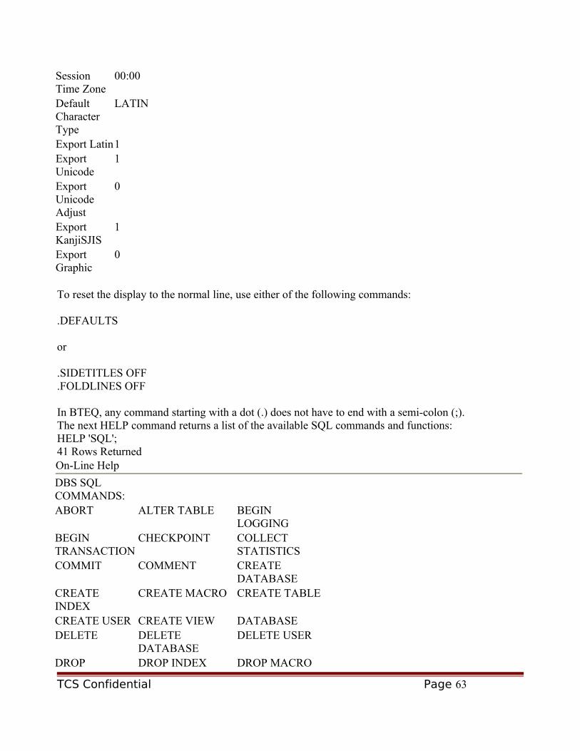
Session Time Zone

00:00


LATIN

Export Latin1Export Unicode

1

Export Unicode Adjust

0

Export KanjiSJIS

1

Export Graphic

0

To reset the display to the normal line, use either of the following commands:

.DEFAULTS

or

.SIDETITLES OFF

.FOLDLINES OFF

In BTEQ, any command starting with a dot (.) does not have to end with a semi-colon (;).The next HELP command returns a list of the available SQL commands and functions:HELP 'SQL';41 Rows ReturnedOn-Line Help

DBS SQL COMMANDS:

ABORT ALTER TABLE BEGIN LOGGING

BEGIN TRANSACTION

CHECKPOINT COLLECT STATISTICS

COMMIT COMMENT CREATE DATABASE

CREATE INDEX

CREATE MACRO CREATE TABLE

CREATE USER CREATE VIEW DATABASEDELETE DELETE

DATABASEDELETE USER

DROP DROP INDEX DROP MACRO

TCS Confidential

On-Line Help

DATABASEDROP TABLE DROP VIEW DROP

STATISTICSECHO END LOGGING END

TRANSACTION.DBS SQL FUNCTIONS:

ABS ADD_MONTHS AVERAGECHARACTERS CAST CHAR2HEXINTCOUNT CORR COVAR_POPCSUM EXP EXTRACTFORMAT INDEX HASHAMPHASHBKAMP HASHBUCKET HASHROWKURTOSIS LN LOGMAVG MAXIMUM MCHARACTERSMDIFF MINDEX MINIMUMMLINREG MSUBSTR MSUMNAMED NULLIFZERO OCTET_LENGTHQUANTILE REGR_INTERCEPT REGR_SLOPERANDOM RANK SKEWSQRT STDDEV_POP STDDEV_SAMPSUBSTR SUM TITLETRIM TYPE UPPERVARGRAPHIC VAR_POP VAR_SAMPZEROIFNULL

The above output is not a complete list of the commands. The three dots in the center represent the location where commands were omitted so it fit onto a single page. All commands are seen when performed on a terminal.Once this output has been used to find the command, than the following HELP command provides additional information on it:

HELP 'SQL END TRANSACTION' ;5 Rows ReturnedOn-Line Help

{ END TRANSACTION }{ } ;{ ET }

Since the terminal is used most of the time to access the database, take advantage of it and use the terminal for your HELP commands.

TCS Confidential

Tools like Queryman also have a variety of HELP commands and individual menus. Always look for ways to make the task easier.

SET SESSION command

The Teradata Database provides user access only by allocating a session with a Parsing Engine. The Parsing engine will use default attributes based on the user and host computer from which the user is connecting. When a different session option is needed, the SET SESSION command is needed. It over-rides the default for this session only. The next time the user logs into Teradata, the original default will be used again.

Syntax for SET SESSION:

SET SESSION { COLLATION <collation-sequence> | ACCOUNT=<account-id> FOR { REQUEST | SESSION } | DATEFORM = { INTEGERDATE | ANSIDATE } | DATABASE <database-name> } ;

The SET SESSION can be abbreviated as: SS.Collation sequence: ASCII, EBCDIC, MULTINATIONAL (European (diacritical) character or Kanji character), CHARSET_COLL (binary ordering based on the current client character set), JIS_COLL (logical ordering of characters based on the Japanese Industrial Standards collation), HOST (EBCDIC for IBM channel-attached clients and ASCII for all other clients — default collation).

Account-id: allows for the temporary changing of accounting data for charge back and priority. The account-id specified must be a valid one assigned to the user and the priority can only be down graded.INTEGERDATE: uses the YY/MM/DD format and ANSIDATE uses the YYYY-MM-DD format for a date.

Database-name: becomes the database to use as the current database for SQL operations during this session.

SHOW commands

There are times when you need to recreate a table, view, or macro that you already have, or you need to create another object of the same type that is either identical or very similar to an object that is already created. When this is the case, the SHOW command is a way to accomplish what you need. The intent of the SHOW command is to output the CREATE statement that could be used to recreate the object of the type specified.

Open table as spreadsheet This chart shows the commands and their formats:

SHOW TABLE <table-name> ;

Displays the CREATE TABLE statement needed to create this table.

TCS Confidential

Open table as spreadsheet This chart shows the commands and their formats:

SHOW VIEW <view-name> ; Displays the CREATE VIEW statement needed to create this view.

SHOW MACRO <macro-name> ;

Displays the CREATE MACRO statement needed to create this macro.

SHOW TRIGGER <trigger-name> ;

Displays the CREATE TRIGGER statement needed to create this trigger.

SHOW PROCEDURE <procedure-name> ;

Displays the CREATE PROCEDURE statement needed to create this stored procedure.

SHOW <SQL-statement> ; Displays the CREATE TABLE statements for all tables/views referenced by the SQL statement .

Figure 3-3

We will be discussing all of these object types and their associated Data Definition Language (DDL) commands later in this course.

To see the CREATE TABLE command for the Employee table, we use the command:

SHOW TABLE Employee ;

13 Rows Returned

CREATE SET TABLE MJL.Employee ,NO FALLBACK ,

NO BEFORE JOURNAL,

NO AFTER JOURNAL

(

Emp_Nbr INTEGER,

Last_Name CHAR(30) CHARACTER SET LATIN NOT CASESPECIFIC NOT NULL,

First_Name VARCHAR(20) CHARACTER SET LATIN NOT CASESPECIFIC NOT NULL,

Social_Sec_Nbr INTEGER,

Birth_Date DATE NOT NULL,

Department_Nbr SMALLINT,

Job_Nbr INTEGER,

Salary DECIMAL(10,2) NOT NULL)

UNIQUE PRIMARY INDEX (Emp_Nbr);

To see the CREATE VIEW command, we use a command like:

SHOW VIEW TODAY ;

3 Rows Returned

CREATE VIEW MJL.TODAY AS

SELECT * FROM SYS_CALENDAR.CALENDAR

WHERE CALENDAR_DATE = '2001-09-21';

TCS Confidential


To see the CREATE MACRO command for the macro called MYREPORT, we use a command like:

SHOW MACRO MYREPORT ;

9 Rows Returned

CREATE MACRO MJL01.MYREPORT (INPARM1 INTEGER, INPARM2 CHAR(10)) AS

(SELECT DEPT,

DAY_OF_WEEK,

AVG(SAL)

FROM SYS_CALENDAR.CALENDAR SC, MYTABLE

WHERE CALENDAR_DATE = :INPARM2 (DATE, FORMAT 'YYYYMMDD')

AND DEPT = :INPARM1

GROUP BY 1,2;);

To see the CREATE TRIGGER command for AVG_SAL_T, we use:

SHOW TRIGGER AVG_SAL_T ;

20 Rows Returned

CREATE TRIGGER MJL.AVG_SAL_T

AFTER UPDATE OF (SALARY) ON MJL.EMPLOYEE

REFERENCING OLD AS OLDROW

NEW AS NEWROW

FOR EACH ROW

WHEN (NEWROW.SALARY >

(SELECT AVG(BUDGET) * .10 (DECIMAL(10,2))

FROM MJL01.DEPARTMENT) )

(INSERT INTO MJL01.GREATER_10_PERCENT

(EMP_NUM

,SAL_DATE

,OLDSAL

,NEWSAL

,PERC_OF_BUDGET)

VALUES (NEWROW.EMP_NBR

,CURRENT_DATE

,OLDROW.SALARY

,NEWROW.SALARY);

) ;

Since the SHOW command returns the DDL, it can be a real time saver. It is a very helpful tool when a database object needs to be recreated, a copy of an existing object is needed, or another object is needed that has similar characteristics to an existing object. Plus, what a great way to get a reminder on the syntax needed for creating a table, view, macro, or trigger.

TCS Confidential

It is a good idea to save the output of the SHOW command in case it is needed at a later date. However, if the object's structure changes, the SHOW command should be re-executed and the new output saved. It returns the DDL that can be used to create a new table exactly the same as the current table. Normally, at a minimum, the table name is changed before executing the command.

EXPLAIN

The EXPLAIN command is a powerful tool provided with the Teradata database. It is designed to provide an English explanation of what steps the AMP must complete to satisfy the SQL request. The EXPLAIN is based on the PE's execution plan.

The Parsing Engine (PE) does the optimization of the submitted SQL, the creation of the AMP steps and the dispatch to any AMP involved in accessing the data. The EXPLAIN is an SQL modifier; it modifies the way the SQL operates.

When an SQL statement is submitted using the EXPLAIN, the PE still does the same optimization step as normal. However, instead of building the AMP steps, it builds the English explanation and sends it back to the client software, not to the AMP. This gives users the ability to see resource utilization, use of indices, and row and time estimates.

Therefore, it can predict a Cartesian product join in seconds, instead of hours later when the user gets suspicious that the request should have been finished. The EXPLAIN should be run every time changes to an object's structure occur, when a request is first put into production and other key times during the life of an application. Some companies require that the EXPLAIN always be run before execution of any new queries.

The syntax for using the EXPLAIN is simple: just type the EXPLAIN keyword preceding your valid SQL statement. For example:

EXPLAIN

<SQL-command> ;

The EXPLAIN can be used to translate the actions for all valid SQL. It cannot provide a translation when syntax errors are present. The SQL must be able to execute in order to be explained.

Open table as spreadsheet Chart for some of the keywords that may be seen in the output of an EXPLAIN:

Locking Pseudo Table Serial lock on a symbolic table. Every table has one. Used to prevent deadlocks situations between users.

Locking table for Indicates that an ACCESS, READ, WRITE, or EXCLUSIVE lock has been placed on the table

Locking rows for <type> Indicates that an ACCESS, READ, or WRITE, lock is placed on rows as they are read or written

Do an ABORT test Guarantees a transaction is not in progress for this user

All AMPs retrieve All AMPs are receiving the AMP steps and are involved in providing the answer set

By way of an all rows scan

Rows are read sequentially on all AMPs

TCS Confidential

Open table as spreadsheet Chart for some of the keywords that may be seen in the output of an EXPLAIN:

By way of primary index Rows are read using the Primary index column(s)

By way of index number Rows are read using the Secondary index — number from HELP INDEX

BMSMS Bit Map Set Manipulation Step, alternative direct access technique when multiple NUSI columns are referenced in the WHERE clause

Residual conditions WHERE clause conditions, other than those of a join

Eliminating duplicate rows

Providing unique values, normally result of DISTINCT, GROUP BY or subquery

Where unknown comparison will be ignored

Indicates that NULL values will not compare to a TRUE or FALSE. Might be seen in a subquery using NOT IN or NOT = ALL because no rows will be returned if comparison is ignored.

Nested join The fastest join possible. It uses a UPI to retrieve a single row after using a UPI or a USI in the WHERE to reduce the join to a single row.

Merge join Rows of one table are matched to the other table on common domain columns after being sorted into the same sequence, normally Row Hash

Product join Rows of one table are matched to all the rows of the other table without concern for a domain match

ROWID join The newest (V2R6) and other fastest join possible. It uses the ROWID of a UPI to retrieve a single row after using a UPI or a USI in the WHERE to reduce the join to a single row.

Duplicated on all AMPs Participating rows for the table (normally smaller table) of a join are duplicated on all AMPS

Hash redistributed on all AMPs

Participating rows of a join are hashed on the join column and sent to the same AMP that stores the matching row of the table to join

SMS Set Manipulation Step, result of an INTERSECT, UNION, EXCEPT or MINUS operation

Last use SPOOL file is no longer needed after the step and space is released

Built locally on the AMPs As rows are read, they are put into SPOOL on the same AMP

Aggregate Intermediate Results are computed locally

The aggregation values are all on the same AMP and therefore no need to redistribute them to work with rows on other AMPs

Aggregate Intermediate Results are computed globally

The aggregation values are not all on the same AMP and must be redistributed on one AMP, to accompany the same value with from the other AMPs

TCS Confidential


Figure 3-4

Once you attain more experience with Teradata and SQL, these terms lead you to a more detailed understanding of the work involved in any SQL request.

The following charts list the confidence levels indicated by the optimizer:

Open table as spreadsheet This chart is for phrases that accompany the estimated number of rows:

No confidence

The PE has no degree of certainty with the values used. This is normally a result of not collecting STATISTICS and working with multiple steps in SPOOL

Low confidence

The PE is not sure of the values being used. This is normally a result of processing involving several steps in SPOOL instead of the actual rows in a table

High confidence

Normally indicates that STATISTICS have been collected on the columns or indices of a table. Allows the optimizer to be more aggressive in the access plan.

Index Join confidence

Indicates that a join is being done there uses a join condition via a unique index.

Figure 3-5

The first is the estimated number of rows that will be returned. This number is an educated guess that the PE has made based on information available at the time of the EXPLAIN. This number may or may not be accurate. If there are current STATISTICS on the table, the numbers are more accurate. Otherwise, the PE calculates a guess by asking a random AMP for the number of rows it contains. Then, it multiples the answer by the number of AMPs to guess a "total row count." At the same time, it lets you know how accurate the number provided might be using the terms in the next chart.

The second area to check in the output of the EXPLAIN is the estimated cost, expressed in time, to complete the SQL request. Although it is expressed in time, do not confuse it with either wall-clock or CPU time. It is strictly a cost factor calculated by the optimizer for comparison purposes only. It does not take the number of users, the current workload or other system related factors into account. After looking at the potential execution plans, the plan with the lowest cost value is selected for execution. Once these two values are checked, the question that should be asked is: Are these values reasonable?

For instance, if the table contains one million rows and the estimate is one million rows in 45 seconds, that is probably reasonable if there is not a WHERE clause. However, if the table contains a million rows and is being joined to a table with two thousand rows and the estimate is that two hundred trillion rows will be returned and it will take fifty days, this is not reasonable.

The following EXPLAIN is for a full table scan of the Student Table:

EXPLAIN

SELECT * FROM Student_table ;

12 Rows Returned

TCS Confidential


Explanation

1. First, we lock a distinct MIKEL."pseudo table" for read on a RowHash to prevent global deadlock for MIKEL.Student_table.

2. Next, we lock MIKEL.Student_table for read.3. We do an all-AMPs RETRIEVE step from MIKEL.Student_table by way of an all-rows scan

with no residual conditions into Spool 1, which is built locally on the AMPs. The size of Spool 1 is estimated with low confidence to be 8 rows. The estimated time for this step is 0.15 seconds.

4. Finally, we send out an END TRANSACTION step to all AMPs involved in processing the request.

-> The contents of Spool 1 are sent back to the user as the result of statement 1. The total estimated time is 0.15 seconds.

The EXPLAIN estimates, 8 rows and .15 seconds. Since there are 10 rows in the table, the EXPLAIN is slightly off in its estimate. However, this is reasonable based on the contents of the table and the SELECT statement submitted.

The next EXPLAIN is for a join that has an error in it, can you find it?:

EXPLAIN

SELECT *

FROM Student_table S, Course_table C, Student_Course_table SC

WHERE s.student_id = sc.student_id ;

Explanation

1. First, we lock a distinct MIKEL."pseudo table" for read on a RowHash to prevent global deadlock for MIKEL.SC.

2. Next, we lock a distinct MIKEL."pseudo table" for read on a RowHash to prevent global deadlock for MIKEL.C.

3. We lock a distinct MIKEL."pseudo table" for read on a RowHash to prevent global deadlock for MIKEL.S.

4. We lock MIKEL.SC for read, we lock MIKEL.C for read, and we lock MIKEL.S for read.5. We do an all-AMPs JOIN step from MIKEL.SC by way of a RowHash match scan with no

residual conditions, which is joined to MIKEL.S. MIKEL.SC and MIKEL.S are joined using a merge join, with a join condition of ("MIKEL.S.Student_ID = MIKEL.SC.Student_ID"). The result goes into Spool 2, which is duplicated on all AMPs. The size of Spool 2 is estimated with low confidence to be 128 rows. The estimated time for this step is 0.19 seconds.

6. We do an all-AMPs JOIN step from MIKEL.C by way of an all-rows scan with no residual conditions, which is joined to Spool 2 (Last Use). MIKEL.C and Spool 2 are joined using a product join, with a join condition of ("(1=1)"). The result goes into Spool 1, which is built locally on the AMPs. The size of Spool 1 is estimated with low confidence to be 512 rows. The estimated time for this step is 0.20 seconds.

7. Finally, we send out an END TRANSACTION step to all AMPs involved in processing the request.

-> The contents of Spool 1 are sent back to the user as the result of statement 1. The total estimated time is 0.39 seconds.

TCS Confidential

The EXPLAIN estimates nearly 512 rows will be returned and it will take .39 seconds. Although the time estimate sounds acceptable, this is a very small table. Looking at the number of rows returned as 512 with only 14 rows in the largest of these tables. This is not reasonable based on the contents of the tables.

Upon further examination, the product join in step 6 is using (1=1) as the join condition where it should be a merge join. Therefore, this is a Cartesian product join. A careful analysis of the SELECT shows a single join condition in the WHERE clause. However, this is a three-table join and should have two join conditions. The WHERE clause needs to be fixed and by using the EXPLAIN we have saved valuable time.

If you can get to the point of using the EXPLAIN in this manner, you are way ahead of the game. No one will ever have to slap your hand for writing SQL that runs for days, uses up large amounts of system resources and accomplishes absolutely nothing. You say, "Doctor, it hurts when I do this." The Doctor says, "Don't do that." We are saying, "Don't put extensive SELECT requests into production without doing an EXPLAIN on it.

Remember, always examine the EXPLAIN for reasonable results. Then, save the EXPLAIN output as a benchmark against any future EXPLAIN output. Then, if the SQL starts executing slower or using more resources, you have a basis for comparison. You might also use the benchmark if you decide to add a secondary index. This prototyping allows you to see exactly what your SQL is doing.

Some users have quit using the EXPLAIN because they have gotten inaccurate results. From our experience, when the numbers are consistently different than the actual rows being returned and the cost estimate is completely wrong, it is normally an indicator that STATISTICS should be collected or updated on the involved tables.

Adding Comments

Sometimes it is necessary or desirable to document the logic used in an SQL statement within the query. A comment is not executed and is ignored by the PE at syntax checking and resolution time.

ANSI Comment

To comment a line using the ANSI standard form of a comment: -- the double dash at the start of a single line denotes a comment is on that line

Each line that is a comment must be started with the same two dashes for each comment line. This is the only technique available for commenting using ANSI compliancy.

At the writing of this book, Queryman sometimes gets confused and regards all lines after the - - as part of the comment. So, be careful regarding various client tools.

-- This is an ANSI form of comment that consists of a single line of user explanation or -- add notes to an SQL command. This is a second line and needs additional dashes

Teradata Comment

To comment a line using the Teradata form of a comment: /* the slash asterisk at the start of a line denotes the beginning of a comment */ the asterisk slash (reversed from the start of a comment) is used to end a comment.

TCS Confidential

Both the start and the end of a comment can be a single line or multiple lines. This is the most common form of comment seen in Teradata SQL, primarily since it was the original technique available.

/* This is the Teradata form of comment that consists of a single line of user explanation or add notes to an SQL command. Several lines of comment can be added within a single notation. This is the end of the comment. */

User Information Functions

The Teradata RDBMS (Relational DataBase Management System) has incorporated into it functions that provide data regarding a user who has performed a logon connection to the system. The following functions make that data available to a user for display or storage.

ACCOUNT Function

Compatibility: Teradata Extension

A user within the Teradata database has an account number. This number is used to identify the user, provide a basis for charge back, if desired and establish a basic priority.

Previously, this number was used exclusively by the database administrator to control and monitor access to the system. Now, it is available for viewing by the user via SQL.

Syntax for using the ACCOUNT function:

SEL[ECT] ACCOUNT ;

As an example, the following returns the account information for my user:

SELECT ACCOUNT;

1 Row returned

ACCOUNT

$M13678

If your account starts with a $M, you are running at a medium priority. Where $L is low and $H is high. At the same time, the account does not have to begin with one of these and can be any site specific value.

DATABASE Function

Compatibility: Teradata ExtensionChapter 1 of this book discussed the concept of a database and user area within the Teradata RDBMS. Knowing the current database within Teradata is sometimes an important piece of information needed by

TCS Confidential


a user. As mentioned above, the HELP SESSION is one way to determine it. However, a lot of other information is also presented. Sometimes it is advantageous to have only that single tidbit of data not only to see but also for storage. When this is the case, the DATABASE function is available.

Syntax for using the DATABASE function:

SEL[ECT] DATABASE ;


SELECT DATABASE;

1 Row returned

DATABASE

Mikel

SESSION Function

Compatibility: Teradata ExtensionChapter 1 of this book discussed the PEP and the concept of a session and its role involving the user's SQL requests. The HELP SESSION provides a wealth of information regarding the individual session established for a user. One of those pieces of data is the session number. It uniquely identifies every user session in existence at any point in time. Teradata now makes the session number available using SQL.

Syntax for using the SESSION function:

SEL[ECT] SESSION ;


SELECT SESSION;

1 Row returned

SESSION

1059

TCS Confidential


Chapter 4: Data Conversions

Data Conversions

In order for data to be managed and used, it must have characteristics associated with it. These characteristics are called attributes that include a data type and a length. The values that a column can store are directly related to these two attributes.

There are times when the data type or length defined is not convenient for the use or output display needed. For instance, when character data is too long for display, an option might be to reduce its length. At other times, the defined numeric data type is not sufficient to store the result of a mathematical operation. Therefore, conversion to a larger numeric type may be the only way to successfully complete the request.

When one of these situations interrupt the execution of the SQL, it is necessary to use one or more of the conversion techniques. They are covered here in detail to enhance the understanding and the use of these capabilities.

In normal practices, there should be little need to convert from a number to a character on a regular basis. This requirement is one indicator that the table or column design is questionable. However, if a conversion must be performed, it is much safer to use the ANSI Standard CAST (Convert And Store) function when going from numeric to character instead of the older Teradata implied conversion. Both of these techniques are discussed here.

Conversions should be used only when absolutely necessary because they are intensive on system resources. As an example, I saw an SQL statement that converted four columns six different times. There were around a million rows in the table. The SQL did a lot of processing and it took about one hour to run. By eliminating these 6 million conversions, the SQL ran in under five minutes. Conversions can have an impact, but sometimes you need them. Use them only when absolutely necessary!

Data Types

Teradata supports many formats for storing data on disk and most of the data types conform to the ANSI standard. At the same time, there are data types specific to Teradata. Most of these unique data types are provided to save storage space on disk or support an international code set.

Since Teradata was originally designed to store terabytes worth of data in millions or billions of rows, saving a single byte one million times becomes a space savings of nearly a megabyte. The savings

TCS Confidential

increases dynamically as more rows are added and more bytes per row are saved. This space savings can be very significant.

Likewise, the speed advantage associated with smaller rows cannot be ignored. Since data is read from a disk in a block, smaller rows mean that more rows are stored in a single block. Therefore, fewer blocks need to be read and it is faster.

The following charts indicate the data types currently supported by Teradata. The first chart shows the ANSI standard types and the second is for the additional data types that are extensions to the standard.

Open table as spreadsheet This chart indicates which data types that Teradata currently supports as ANSI Standards:

Data Type Description Data Value Range

INTEGER Signed whole number -2,147,483,648 to 2,147,483,647

SMALLINT Signed smaller whole number

-32,768 to 32,767

DECIMAL(X,Y)

Where: X=1 thru 18, total number of digits in the number And Y=0 thru 18 digits to the right of the decimal

Signed decimal number 18 digits on either side of the decimal point

Largest value DEC(18,0)

Smallest value DEC(18,18)

NUMERIC(X,Y)

Same as DECIMAL

Synonym for DECIMAL Same as DECIMAL

FLOAT | REAL | PRECISION | DOUBLE PRECISION

Floating Point Format (IEEE)

<value>x10307 to <value>x10-308

CHARACTER(X)

CHAR(X)

Where: x=1thru 64000

Fixed length character string, 1 byte of storage per character,

1 to 64,000 characters long, pads to length with space

VARCHAR(X)

CHARACTER VARYING(X)

CHAR VARYING(X)

Where: X=1 thru 64000

Variable length character string, 1 byte of storage per character, plus 2 bytes to record length of actual data

1 to 64,000 characters as a maximum. The system only stores the characters presented to it.

CLOB (X { K | M | G })

CHARACTER LARGE

OBJECT (X { K | M | G })

Large character object, for manipulating chunks. Can also specify character set and attribute.

Max for LATIN in K, M or G: 2097088000 bytes

Max for UNICODE in K or M: 1048544000 bytes. See manual.

BLOB (X { K | M | G })

BINARY LARGE OBJECT (X { K | M | G })

Large binary object, for manipulating chunks.

Specified in Kilobytes, Megabytes or Gigabytes. Max is 2097088000 bytes. See manual.

TCS Confidential

Open table as spreadsheet This chart indicates which data types that Teradata currently supports as ANSI Standards:


DATE Signed internal representation of YYYYMMDD

See chapter 8 for details

TIME Identifies a field as a TIME value with Hour, Minutes and Seconds

TIMESTAMP Identifies a field as a TIMESTAMP value with Year, Month, Day, Hour, Minute, and Seconds

Figure 4-1

Open table as spreadsheet This chart indicates which data types that Teradata currently supports as extensions:


BYTEINT Signed whole number -128 to 127

BYTE (X)


Binary 1 to 64,000 bytes

VARBYTE (X)


Variable length binary 1 to 64,000 bytes

LONG VARCHAR Variable length string 64,000 characters (maximum data length) The system only stores the characters provided, not trailing spaces.)

GRAPHIC (X)


Fixed length string of 16-bit bytes (2 bytes per character)

1 to 32,000 KANJI characters

VARGRAPHIC (X)


Variable length string of 16-bit bytes

1 to 32,000 characters as a maximum. The system only stores characters provided.

Figure 4-2

These data types are all available for use within Teradata. Notice that there are fixed and variable length data formats. The fixed data types always require the entire defined length on disk for the column. The variable types can be used to maximize data storage within a block by storing only the data provided within a row by the client software.

TCS Confidential




You should use the appropriate type for the specific data. It is a good idea to use a VAR data type when most of the data is less than the maximum size. This is due to the addition of an extra 2-byte length indicator that is stored along with the actual data.

CAST

Compatibility: ANSI

Under most conditions, the data types defined and stored in a table should be appropriate. However, sometimes it is neither convenient nor desirable to use the defined type. Data can be converted from one type to another by using the CAST function. As long as the data involved does not break any data rules (i.e. placing alphabetic or special characters into a numeric data type) the conversion works. The name of the CAST function comes from the Convert And STore operation that it performs.

Care must also be taken when converting data to manage any potential length issues. In Teradata mode, truncation occurs if a length is requested that is shorter than the original data. However, in ANSI mode, an SQL error is the result because ANSI says, "Thou shall not truncate data."

The basic syntax of the CAST statement follows:

SELECT CAST(<column-name> AS <data-type>[(<length>)])

FROM <table-name> ;

Examples using CAST:

CAST ( <smallint-data> AS CHAR(5) ) /* smallint to character */

CAST ( <decimal-data> AS INTEGER ) /* truncates decimals */

CAST ( <byteint-data> AS SMALLINT ) /* binary to smallint */

CAST ( <char-data> AS BYTE (128) ) /* character to binary */

CAST ( <byteint-data> AS VARCHAR(5) ) /* byteint to character */

CAST ( <integer-data> AS FLOAT) /* integer to float point */

These are only some of the potential conversions and are primarily here for illustration of how to code a CAST. The CAST could also be used within the WHERE clause to control the length characteristics or the type of the data to compare.

Again, when using the CAST in ANSI mode, any attempt to truncate data causes the SQL to fail because ANSI does not allow truncation.

The next SELECT uses literal values to show the results of conversion:

SELECT CAST('ABCDE' AS CHAR(1) ) AS Trunc

,CAST(128 AS CHAR(3) ) AS OK

,CAST(127 AS INTEGER) AS Bigger

,CAST(121.53 AS SMALLINT) AS Whole

,CAST(121.53 AS DECIMAL(3,0)) AS Rounder ;

1 Row Returned

Trunc OK .

Bigger Whole Rounder

A 128 127 121 122

TCS Confidential

In the above example, the first CAST truncates the five characters (left to right) to form the single character 'A'. In the second CAST, the integer 128 is converted to three characters and left justified in the output. The 127 was initially stored in a SMALLINT (5 digits - up to 32767) and then converted to an INTEGER. Hence, it uses 11 character positions for its display, ten numeric digits and a sign (positive assumed) and right justified as numeric.

The value of 121.53 is an interesting case for two reasons. First, it was initially stored as a DECIMAL as 5 total digits with 2 of them to the right of the decimal point. Then it is converted to a SMALLINT using CAST to remove the decimal positions. Therefore, it truncates data by stripping off the decimal portion. It does not round data using this data type. On the other hand, the CAST in the fifth column called Rounder is converted to a DECIMAL as 3 digits with no digits (3,0) to the right of the decimal, so it will round data values instead of truncating. Since .53 is greater than .5, it is rounded up to 122.

Implied CAST


Although the CAST function is the ANSI standard, it has not always been that way. Prior to the CAST function, Teradata had the ability to convert data from one type to another.

This conversion is requested by placing the "implied' data type conversion in parentheses after the column name. Therefore, it becomes a part of the select list and the column request. The new data type is written as an attribute for the column name.

The following is the format for requesting a conversion:

SELECT <column-name> (<data-type> [(<length>)]

FROM <table-name> ;

At first glance, this appears to be the best and shortest technique for doing conversions. However, there is a hidden danger here when converting from numeric to character that is demonstrated in this SELECT that uses the same data as above to do implied CAST conversions:

SELECT 'ABCDE' (CHAR(1)) AS Shortened

,128 (CHAR(3)) AS OOPS1

,-128 (CHAR(3)) AS OOPS2

,128 (INTEGER) AS Bigger

,121.13 (SMALLINT) AS Whole ;

1 Row Returned

Shortened OOPS1 OOPS2 Bigger Whole

A - 128 121

What happened in the column named OK and N_OK?

The answer to this question is: the value 128 is 1 greater than 127 and therefore too large of a value to store in a BYTEINT. So it is automatically stored as a SMALLINT (5 digits plus a sign) before the conversion. The implicit conversion changes it to a character type with the first 3 characters being returned. As a result, only the first 3 spaces are seen in the report (_ _ _ 128). Likewise, OOPS2 is stored as (_ _ -128) with the first three characters (2 spaces and -) shown in the output.

TCS Confidential

Always think about the impact of the sign as a valid part of the data when converting from numeric to character. As mentioned earlier, if you find that conversions of this type are regularly necessary, the table design needs to be re-examined. As demonstrated in the above output, it is always safer to use CAST when going from character to numeric data types.

Formatted Data


Remember that truncation works in Teradata mode, but not in ANSI mode. So, another way to make data appear to be truncated is to use the Teradata FORMAT in the SELECT list with one or more columns when using a tool like BTEQ. Since FORMAT does not truncate data, it works in ANSI mode.

The syntax for using FORMAT is:

SELECT '<char-data>' (FORMAT 'X(4)') /* alphabetic format 4 characters */

,<numeric-data>' (FORMAT '999') /* numeric format characters */

,<date-data> (FORMAT 'YYYY-MM-DD') /* date format characters */

FROM <table-name> ;

The next SELECT demonstrates the use of FORMAT:

SELECT 'ABCDE' (FORMAT 'XXX') AS Shorter

,121.53 (FORMAT '99999') AS Fmt_121

,121.53

,991001(date) (FORMAT 'MM/dd/Yy') AS Fmt_NumDate

,991001(date) (FORMAT 'mmmbdd,byyyy') AS Fmt_Date ;

1 Row Returned

Shorter Fmt_121 121.53 Fmt_NumDate Fmt_Date

ABC 00121 121.53 10/01/99 OCT 01, 1999

There are a couple of things to notice in this output. First, it works in ANSI mode because truncation does not occur. The distinction is that all of the data from the column is in spool. It is only the output that is shortened, not truncated. The character data types use the 'X' for the formatting character.

Second, formatting does not round a data value as with the 121.53, the display is shortened. The numeric data types use a '9' as the basic formatting character. Others are shown in this chapter.

Next, DATE type data uses the 'M' for month, the 'D' for day of the month and 'Y' for the year portion of a valid date. Lastly, the case of the formatting characters does not matter. The formatting characters can be written in all uppercase, lowercase, or a mixture of both cases.

The two following charts show the valid formatting characters for Teradata and provide an explanation of the impact each one has on the output display when using BTEQ:

Basic Numeric and Character Data Formatting Symbols

TCS Confidential

Open table as spreadsheet Symbol

Mask character and how used

X or x Character data. Each X represents one character. Can repeat value- i.e. XXXXX or X(5).

9 Decimal digit. Holds place for numeric digit for a display 0 through 9. All leading zeroes are shown if the format mask is longer than the data value. Can repeat value- i.e. 99999 or 9(5).

V or v Implied decimal point. Aligns data on a decimal value. Primarily used on imported data without actual decimal point.

E or e Exponential. Aligns the end of the mantissa and the beginning of the exponent.

G or g Graphic data. Each G represents one logical (double byte- KANJI or Katakana) character. Can repeat value- i.e. GGGGG or G(5).

Figure 4-3

Open table as spreadsheet Advanced Numeric and Character Formatting Symbols

Symbol Mask character and how used

$ Fixed or floating dollar sign. Inserts a $ or leaves spaces and moves (floats) over to the first character of a currency value. With the proper keyboard, additional currency signs are available: Cent, Pound and Yen.

, Comma. Inserted where appears in format mask. Used primarily to make large numbers easier to read.

. Period. Primary use to align decimal point position. Also used for: dates and comma in some currencies.

- Dash character. Inserted where appears in format mask. Used primarily for dates and negative numeric values. Also used for: phone numbers, zip codes, and social security (USA).

/ Slash character. Inserted where appears in format mask. Used primarily for dates.

% Percent character. Inserted where appears in format mask. Used primarily for display of percentage — i.e. 99% vs. .99

Z or z Zero-suppressed decimal digit. Holds place for numeric digit displays 1 through 9 and 0, when significant. All leading zeroes (insignificant) are shown as space since their presence does not change the value of the number being displayed.

B or b Blank data. Insert a space where appears in format mask.

Figure 4-4

The next chart shows the formatting characters used in conjunction with DATE data:

Open table as spreadsheet Date Formatting Symbols

Symbol Mask character and how used (not case specific)

TCS Confidential




Open table as spreadsheet Date Formatting Symbols

Symbol Mask character and how used (not case specific)

D or d Day. Allows day to be displayed any where in the date display. When 'DD' is specified, the numeric (01–31) value is available. When 'DDD' is specified, the three-digit day of the year (001–366) value is available.

E or e Day of the week. Provides the day of the week as three or four characters. Using 'eee' yields 'Sun' and 'eeee' yields 'Sund' for Sunday.

Y or y Year. Allows day to be displayed any where in the date display. The normal 'YY' has been used for many years for the 20th century with the 19YY assumed. However, since we have moved into the 21st century, it is recommended that the 'YYYY' be used.

Figure 4-5

There is additional information on date formatting in a later chapter dedicated exclusively to date processing.

The next SELECT demonstrates some of the additional formatting symbols:

SELECT 'ABCDE' (FORMAT 'XxX') AS Fmt_Shorter

,2014859999 (FORMAT '999-999-9999') AS Fmt_Phone

,1021.53 (FORMAT 'ZZZZZZ9.9999') AS Z_Press

,991001(date) (FORMAT 'Yyddd') AS Fmt_Julian

,991001(date) (FORMAT 'eee') As Weekday

,991001 (FORMAT '$$$$,$$$.99') AS Fmt_Pay ;

1 Row Returned

Fmt_Shorter Fmt_Phone Z_Press Fmt_Julian Weekday Fmt_Pay

ABC 201-485-9999

1021.53 99274 Fri $991,001.00

There are only two things that need to be watched when using the FORMAT function. First, the data type must match the formatting character used or a syntax error is returned. So, if the data is numeric, use a numeric formatting character and the same condition for character data. The other concern is configuring the format mask big enough for the largest data column. If the mask is too short, the SQL command executes, however, the output contains a series of ************* to indicate a format overflow, as demonstrated by the following SELECT:

SELECT 2014859999 (FORMAT '999-9999') AS Fmt_Phone ;

1 Row Returned

Fmt_Phone

*********

All of these FORMAT requests work wonderfully if the client software is BTEQ. After all, it is a report writer and these are report writer options. The issue is that the ODBC and Queryman look at the data as data, not as a report. Since many of the formatting symbols are "characters" they cannot be numeric. Therefore, the ODBC strips off the symbols and presents the numeric data to the client software for display.

TCS Confidential


Tricking the ODBC to Allow Formatted Data

If a tool uses the ODBC, the FORMAT in the SELECT is ignored and the data comes back as data, not as a formatted field. This is especially noticeable with numeric data and dates.

To force tools like Queryman to format the data, the software must be tricked into thinking the data is character type, which it leaves alone. This can be done using the CAST function.The next SELECT uses the CAST operation to trick the software into thinking the formatted data is character:

SELECT CAST( (4859999 (FORMAT '999-9999') ) AS CHAR(8)) /* explicit CAST */

AS Fmt_CAST_Phone /* implicit cast */

,991001(date) (FORMAT 'yyyy.mm.dd') (CHAR(10) )

AS Fmt_CAST_Date

,CAST((991001 (FORMAT '$$$$,$$$.99')) AS CHAR(11) )

AS Fmt_CAST_Pay ;

1 Row Returned

Fmt_CAST_Phone Fmt_CAST_Date Fmt_CAST_Pay

485–9999 1999.10.01 $991,001.00

Do not let the presence of AS in the above SELECT confuse you. The first AS, inside the parentheses, goes with the new data type for the CAST. Notice that the parentheses enclose both the data and the FORMAT so that they are treated as a single entity. The second AS is outside the parentheses and is used to name the alias.

TITLE Attribute for Data Columns


As seen earlier, an alias may be used to change the column name. This can be done for ease of reference or to alter the heading for the column in the output. The TITLE is an alternative to using an alias name when a column heading needs to be changed. There is a big difference between TITLE and an alias. Although an alias does change the title on a report, it is normally used to rename a column (throughout the SQL) as a new name. The TITLE only changes the column heading.

The syntax for using TITLE follows:

SELECT <column-name> (TITLE 'Column title to appear in output')

, <column-name> (TITLE 'Level 1 // Level 2 // Level 3')

FROM <table-name> ;

Like FORMAT, TITLE changes the attribute of the displayed data. Therefore, it is written in parentheses also. Also like FORMAT, tools using the ODBC may not work as well as they do in BTEQ, the report writer. This is especially true when using the // stacking symbols. In tools like Queryman, the title literally contains // and is probably not the intent. Also, if you attempt to use TITLE in Queryman and it does not work, there is a configuration option in the ODBC. When "Use Column Names" is checked, it will not use the title designation.

The following SELECT uses the TITLE to show the result:

TCS Confidential

SELECT 'Character Data'

, 'Character Data' (TITLE 'Character // Data')

,123 (TITLE 'Numeric Data') ;

1 Row Returned

Character Data

Character Data

Numeric Data

Character Data

Character Data

123

Notice that the word 'Character' is stacked over the 'Data' portion of the heading for the second column using BTEQ. So, as an alternative, a TITLE can be used instead of an alias and allows the user to include spaces in the output title.

Another neat trick for TITLE is to use two single quotes together (TITLE ''). This technique creates a zero length TITLE, or no title at all, as seen in the next SELECT:

SELECT 'Character Data'

, 'Character Data' (TITLE '')

,123 (TITLE '') ;

1 Row Returned

Character Data

Character Data

Character Data

123

Remember, this TITLE is two separate single quotes, not a single double quote. A double quote by itself does not work because it is unbalanced without a second double quote.

Transaction Modes

Transaction mode is an area where the perspective of the Teradata RDMBS and ANSI experience a departure. Teradata, by default, is completely non-case specific. ANSI requires just the opposite condition, everything is case specific and as we saw earlier, dictates that table and column names be in capital letters.

This is probably a little restrictive and I tend to agree completely with the Teradata implementation. At the same time, Teradata allows the user to work in either mode within a session when connected to the RDBMS. The choice is up to the user when BTEQ is the client interface software.

For instance, within BTEQ either of the following commands can be used before logging onto the database:

.SET SESSION TRANSACTION ANSI

or

.SET SESSION TRANSACTION BTET

The BTET transaction is simply an acronym made from a consolidation of the BEGIN TRANSACTION (BT) and END TRANSACTION (ET) commands to represent Teradata mode.

TCS Confidential

When using SQL Assistant, an ODBC can be configured to use the "Mode" of ANSI.

The system administrator defines the system default mode for Teradata. A setting in the DBS Control record determines the default session mode. The above commands allow the default to be over-ridden for each logon session. The SET command must be executed before the logon to establish the transaction mode for the next session(s).

However, not all client software supports the ability to change modes between Teradata and ANSI. When it is desirable for functionality or processing characteristics of the other mode, other options are available and are presented below. There is more information on transactional processing later in this book.

Case Sensitivity of Data

It has been discussed earlier that there is no need for concern regarding the use of lower or upper case characters when coding the SQL. As a matter of fact, the different case letters can be mixed in a single statement. Normally, the Teradata database does not care about the case when comparing the stored data either.

However, the ANSI mode implementation of the Teradata RDBMS is case sensitive, regarding the data. This means that it knows the difference between a lower case letter like 'a' and an upper case letter 'A'. At the same time, when using Teradata mode within the Teradata database, it does not distinguish between upper and lower case letters. It is the mode of the session that dictates the case sensitivity of the data.

The SQL can always execute ANSI standard commands in Teradata mode and likewise, can always execute Teradata extensions in ANSI mode. The SQL is always the same regardless of the mode being used. The difference comes when comparing the results of the data rows being returned based on the mode.

For example, earlier in this chapter, it was stated that ANSI mode does not allow truncation. Therefore, the FORMAT could be used in either mode because it did not truncate data.

To demonstrate this issue, the following uses the different modes in BTEQ:

.set session transaction ansi

.logon user1

SELECT 'They match' (title '') WHERE 'A' = 'a';

No Rows Returned

The above SQL execution is case specific due ANSI mode and 'A' is different than 'a'. The same SQL is executed again here, however, the transaction mode for the session is set to Teradata mode (BTET) prior to the logon:

.set session transaction btet

.logon user1

SELECT 'They match' (title '') WHERE 'A' = 'a';

1 Row Returned

They match

Now that the defaults have been demonstrated, the following functions can be used to mimic the operation of each mode while executing in the other (ANSI vs Teradata) where case sensitivity is concerned.

TCS Confidential

CASESPECIFIC


The CASESPECIFIC attribute may be used to request that Teradata compare data values with a distinction made between upper and lower case. The logic behind this designation is that even in Teradata mode, case sensitivity can be requested to make the SQL work the same as ANSI mode, which is case specific. Therefore, when CASESPECIFIC is used, it normally appears in the WHERE clause.

The syntax of the next two statements execute exactly the same:

SELECT <column-name>

FROM <table-name>

WHERE <column-name>(CASESPECIFIC) = { '<character-literal>' | <column-name> } ;

Or, it may be abbreviated as CS:


FROM <table-name>

WHERE <column-name>(CS) = { '<character-literal>' | <column-name> } ;

Conversely, if ANSI is the current mode and there is a need for it to be non-case specific, the NOT can be used to adjust the default operation of the SQL within a mode.

The following SQL forces ANSI to be non-case specific:


FROM <table-name>

WHERE <column-name> (NOT CASESPECIFIC) =

{ '<character-literal>' | <column-name> } ;

Or, it may be abbreviated as:


FROM <table-name>

WHERE <column-name>(NOT CS) = { '<character-literal>' | <column-name> } ;

The next SELECT demonstrates the functionality of CASESPECIFIC and CS for comparing an equality condition like it executed above in ANSI mode:

.set session transaction btet

.logon user1

SELECT 'They match' (title '') WHERE 'A'(CASESPECIFIC) = 'a'(CS) ;

No Rows Returned

No rows are returned, because 'A' is different than 'a' when case sensitivity is used. At first glance, this seems to be unnecessary since the mode can be set to use either ANSI or Teradata. However, the dot (.) commands are BTEQ commands. They do not work in Queryman. If case sensitivity is needed when using other tools, this is one of the options available to mimic ANSI comparisons while in Teradata mode.

TCS Confidential

The SQL extensions in Teradata may be used to eliminate the absolute need to log off to reset the mode and then log back onto Teradata in order to use a characteristic like case sensitivity. Instead, Teradata mode can be forced to use a case specific comparison, like ANSI mode by incorporating the CASESPECIFIC (CS) into the SQL. The case specific option is not a statement level feature; it must be specified for each column needing this type of comparison in both BTEQ and Queryman.

LOWER Function

Compatibility: ANSI

The LOWER case function is used to convert all characters stored in a column to lower case letters for display or comparison. It is a function and therefore requires that the data be passed to it.

The syntax for using LOWER:

SELECT LOWER(<column-name>)

FROM <table-name>

WHERE LOWER(<column-name>) = { '<character-literal>' | <column-name> } ;

The following SELECT uses an upper case literal value as input and outputs the same value, but in lower case:

SELECT LOWER ('ABCDE') AS Result ;

1 Row Returned

Result

abcde

When LOWER is used in a WHERE clause, the result is a predictable string of all lowercase characters. When compared to a lowercase value, the result is a case blind comparison. This is true regardless of how the data was originally stored.

SELECT 'They match' (title 'Do they match?')

WHERE LOWER('aBcDe') = 'abcde' ;

1 Row Returned

Do They match?

They match

UPPER Function

Compatibility: ANSI

The UPPER case function is used to convert all characters stored in a column to the same characters in upper case. It is a function and therefore requires that data be passed to it.

The syntax for using UPPER:

SELECT UPPER(<column-name>)

FROM <table-name>

WHERE UPPER(<column-name>) = { '<character-literal>' | <column-name> } ;

TCS Confidential

The next example uses a literal value within UPPER to show the output all in upper case:

SELECT UPPER('aBcDe') AS Result ;

1 Row Returned

Result

ABCDE

It is also possible to use both the LOWER and UPPER case functions within the WHERE clause. This technique can be used to make ANSI non-case specific, like Teradata, by converting all the data to a known state, regardless of the starting case. Thus, it does not check the original data, but instead it checks the data after the conversion.

The following SELECT uses the UPPER function in the WHERE:

SELECT'They match' (title 'Do they match?')

WHERE UPPER('aBcDe') = 'ABCDE' ;

1 Row Returned

Do They match?

They match

When the data does not meet the requirements of the output format, it is time to convert the data. The UPPER and LOWER functions can be used to change the appearance or characteristics of the data to a known state.

When case sensitivity is needed, ANSI is one way to accomplish it. If that is not an option, the CASESPECIFIC function can be incorporated into the SQL.

TCS Confidential

Chapter 5: Aggregation

Aggregate Processing

The aggregate functions are used to summarize column data values stored in rows. Aggregates eliminate the detail information from the rows and only return the answer. Therefore, the result is one or more aggregated values as a single line or one line per unique value, as a group. The other characteristic of these functions is that they all ignore null values stored in column data passed to them.

Math Aggregates

The math aggregates are the original functions used to provide simple types of arithmetic operations for the data values. Their names are descriptive of the operation performed. The functions are listed below with examples following their descriptions. The newer, V2R4 statistical aggregates are covered later in this chapter.

The SUM Function

Accumulates the values for the named column and prints one total from the addition.

The AVG Function

Accumulates the values for the named column and counts the number of values added for the final division to obtain the average.

The MIN Function

Compares all the values in the named column and returns the smallest value.

The MAX Function

Compares all the values in the named column and returns the largest value.

TCS Confidential

The COUNT Function

Adds one to the counter each time a value other than null is encountered.

The aggregates can all be used together in a single request on the same column, or individually on different columns, depending on your needs.

The following syntax shows all six aggregate functions in a single SELECT to produce a single line answer set:

SELECT SUM(<column-name>)

,AVG(<column-name>)

,MIN(<column-name>)

,MAX(<column-name>)

,COUNT(<column-name>)

FROM <table-name>

[ GROUP BY ]

[HAVING <aggregated-value> <comparison-test> <value> ]

;

The following table is used to demonstrate the aggregate functions:

Figure 5-1

The next SELECT uses the Student table, to show all aggregates in one statement working on the same column:

SELECT SUM(Grade_pt)

,AVG(Grade_pt)

,MIN(Grade_pt)

,MAX(Grade_pt)

,COUNT(Grade_pt)

FROM Student_table;

1 Row Returned

SUM(Grade_pt) AVG(Grade_pt) MIN(Grade_pt) MAX(Grade_pt) COUNT(Grade_pt)

24.88 2.76 0.00 4.00 9

Notice that Stanley's row is not included in the functions due to the null in his grade point average. Also notice that no individual grade point data is displayed because the aggregates eliminate this level of

TCS Confidential

column and row detail and only returns the summarized result for all included rows. The way to eliminate rows from being included in the aggregation is through the use of a WHERE clause.

Since the name of the selected column appears as the heading for the column, aggregate names make for funny looking headings. To make the output look better, it is a good idea to use an alias to dress up the name used in the output. Additionally, the alias can be used elsewhere in the SQL as the column name.

The next SELECT demonstrates the use of alias names for the aggregates:

SELECT SUM(Grade_Pt) AS "Total"

,AVG(Grade_Pt) AS "Average"

,MIN(Grade_Pt) AS Smallest

,MAX(Grade_Pt) AS Highest

,COUNT(Grade_Pt) AS "Count"

FROM Student_table ;

1 Row Returned

Total Average Smallest Largest Count

24.88 2.76 0.00 4.00 9

Notice that when using aliases in the above SELECT they appear as the heading for each column. Also the words Total, Average and Count are in double quotes. As mentioned earlier in this book, the double quoting technique is used to tell the PE that this is a column name, opposed to being the reserved word. Whereas, the single quotes are used to identify a literal data value.

Aggregates and Derived Data

The various aggregates can work on any column. However, most of the aggregates only work with numeric data. The COUNT function might be the primary one used on either character or numeric data. The aggregates can also be used with derived data.

The following table is used to demonstrate derived data and aggregation:

Figure 5-2

This SELECT totals the salaries for all employees and show what the total salaries will be if everyone is given a 5% or a 10% raise:

SELECT SUM(salary) (Title 'Salary Total', Format '$$$$,$$9.99')

,SUM(salary*1.05) (Title '+5% Raise', Format '$$$$,$$9.99')

,SUM(salary*1.10) (Title '+10% Raise', format '$$$$,$$9.99')

,AVG(salary) (Title 'Average Salary', format '$$$$,$$9.99')

TCS Confidential

,SUM(salary) / COUNT(salary) (Title 'Computed Average Salary')

( format '$$$$,$$9.99')

FROM Employee_table;

1 Row Returned

Salary Total

+5% Raise +10% Raise_

Average Salary

Computed Average Salary

$421,039.38 $442,091.35 $463,143.32 $46,782.15 $46,782.15

Notice that since both TITLE and FORMAT require parentheses, they can share the same set. Also, the AVG function and dividing the SUM by the COUNT provide the same answer.

GROUP BY

It has been shown that aggregates produce one row of output with one value per aggregate. However, the above SELECT is inconvenient if individual aggregates are needed based on different values in another column, like the class code. For example, you might want to see each aggregate for freshman, sophomores, juniors, and seniors.

The following SQL might be run once for each unique value specified in the WHERE clause for class code, here the aggregates only work on the senior class (‘SR’):

SELECT SUM(Grade_Pt) AS "Total"





FROM Student_table

WHERE class_code = 'SR' ;

1 Row Returned

Total Average Smallest Largest Count

6.35 3.175 3.00 3.35 2

Although this technique works for finding each class, it is not very convenient. The first issue is that each unique class value needs to be known ahead of time for each execution. Second, each WHERE clause must be manually modified for the different values needed. Lastly, each time the SELECT is executed, it produces a separate output. In reality, it might be better to have all the results in a single report format.

Since the results of aggregates are incorporated into a single output line, it is necessary to create a way to provide one line returned per a unique data value. To provide a unique value, it is necessary to select a column with a value that groups various rows together. This column is simply selected and not used in an aggregate. Therefore, it is a not an aggregated column.

However, when aggregates and "non-aggregates" (normal columns) are selected at the same time, a 3504 error message is returned to indicate the mixture and that the non-aggregate is not part of an associated group. Therefore, the GROUP BY is required in the SQL statement to identify every column selected that is not an aggregate.

TCS Confidential

The resulting output consists of one line for all aggregate values for each unique data value stored in the column(s) named in the GROUP BY. For example, if the department number is used from the Employee table, the output consists of one line per department with at least one employee working in it.

The next SELECT uses the GROUP BY to create one line of output per unique value in the class code column:

SELECT Class_code

,SUM(Grade_Pt) AS "Total"





FROM Student_table

GROUP BY Class_code ;

5 Rows Returned

Class_code Total Average Smallest Largest Count

FR 6.88 2.29 0.00 4.00 2

? ? ? ? ? 0

JR 5.85 2.925 1.90 3.95 2

SR 6.35 3.175 3.00 3.35 2

SO 5.80 2.9 2.00 3.80 2

Notice that the null value in the class code column is returned. At first, this may seem contrary to the aggregates ignoring nulls. However, class code is not being aggregated and is selected as a "unique value." All the aggregate values on the grade point for this row are null, except for COUNT. Although, the COUNT is zero and this does indicate that the null value is ignored. The COUNT value initially starts at zero, so: 0 + 0 = 0.

The GROUP BY is only required when a non-aggregate column is selected along with one or more aggregates. Without both a non-aggregate and a GROUP BY clause, the aggregates return only one row. Whereas, with a non-aggregate and a GROUP BY clause designating the column(s), the aggregates return one row per unique value in the column, as seen above.

Additionally, more than one non-aggregate column can be specified in the SELECT and in the GROUP BY clause. The normal result of this is that more rows are returned. This is because one row appears whenever any single column value changes, the combination of each column constitutes a new value. Remember, all non-aggregates selected with an aggregate must be included in the GROUP BY, or a 3504 error is returned.

As an example, the last name might be added as a second non-aggregate. Then, each combination of last name and class code are compared to other students in the same class. This combination creates more lines of output. As a result, each aggregate value is primarily the aggregation of a single row. The only time multiple rows are processed together is when multiple students have the same last name and are in the same class. Then they group together based on the values in both columns being equal.

This SELECT demonstrates the correct syntax when using multiple non-aggregates with aggregates and the output is one line of output for each student:

TCS Confidential

SELECT Last_name

,Class_code






FROM Student_table

GROUP BY 1, 2 ;

10 Rows Returned

Last_name Class_code Total Average Smallest Largest Count

Johnson ? ? ? ? ? 0

Thomas FR 4.00 4.00 4.00 4.00 1

Smith SO 2.00 2.00 2.00 2.00 1

McRoberts JR 1.90 1.90 1.90 1.90 1

Larkins FR 0.00 0.00 0.00 0.00 1

Phillips SR 3.00 3.00 3.00 3.00 1

Delaney SR 3.35 3.35 3.35 3.35 1

Wilson SO 3.80 3.80 3.80 3.80 1

Bond JR 3.95 3.95 3.95 3.95 1

Hanson FR 2.88 2.88 2.88 2.88 1

Beyond showing the correct syntax for multiple non-aggregates, the above output reveals that it is possible to request too many non-aggregates. As seen above, every output line is a single row. Therefore, every aggregated value consists of a single row. Therefore, the aggregate is meaningless because it is the same as the original data value. Also notice that without an ORDER BY, the GROUP BY does not sort the output rows.

Like the ORDER BY, the number associated with the column's relative position within the SELECT can also be used in the GROUP BY. In the above example, the two columns are the first ones in the SELECT and therefore, it is written using the shorter format: GROUP BY 1,2.

Caution: Using the shorter technique can cause problems if the location of a non-aggregate is changed in the SELECT list and the GROUP BY is not changed. The most common problem is a 3504 error message indicating that a non-aggregate is not included in the GROUP BY, so the SELECT does not execute.

As previously shown, the default for a column heading is the column name. It is not very pretty to see the name of the aggregate and column used as a heading. Therefore, an alias is suggested in all tools or optionally, a TITLE in BTEQ to define a heading.

Also seen earlier, a COUNT on the grade point for department null is zero. Actually, this is misleading in that 1 row contains a null not zero rows. But, because of the null value, the row is not counted. A better technique might be the use of COUNT(*), for a row count. Although this implies counting all columns, in reality it counts the row. The objective of this request is to find any column that contains a non-null data value.

TCS Confidential

Another method to provide the same result is to count any column that is defined as NOT NULL. However, since it takes time to determine such a column and its name is longer than typing an asterisk (*), it is easier to use the COUNT(*).

Again, the GROUP BY clause creates one line of output per unique value, but does not perform a sort. It only creates the distinct grouping for all of the columns specified. Therefore, it is suggested that you always include an ORDER BY to sort the output.

The following might be a better way to code the previous request, using the COUNT(*) and an ORDER BY:

SELECT Class_code





,COUNT(*) AS "Count"

FROM Student_table

GROUP BY 1

ORDER BY 1 ;

5 Rows Returned

Class_code Total Average Smallest Largest Count

? ? ? ? ? 1

FR 6.88 2.29 0.00 4.00 3

JR 5.85 2.925 1.90 3.95 2

SO 5.80 2.9 2.00 3.80 2

SR 6.35 3.175 3.00 3.35 2

Now the output is sorted by the class code with the null appearing first, as the lowest "value." Also notice the count is one for the row containing mostly NULL data. The COUNT(*) counts the row.

Limiting Output Values Using HAVING

As in any SELECT statement, a WHERE clause can always be used to limit the number or types of rows used in the aggregate processing. Therefore, something besides a WHERE is needed to evaluate aggregate values because the aggregate is not finished until all eligible rows have been read. Again, a WHERE clause eliminates rows during the process of reading the base table rows. To allow for the elimination of specific aggregate results, the HAVING clause is used to make the final comparison before the aggregate results are returned.

The previous SELECT is modified below to compare the aggregates and only return the students from spool with a grade point average of B (3.0) or better:

TCS Confidential

SELECT Class_code




FROM Student_table

HAVING "Average" > 3.00

GROUP BY 1

ORDER BY 1;

1 Rows Returned

Class_code Total Average Count

SR 6.35 3.18 2

Notice that all of the previously seen output with an average value less than 3.00 has been eliminated as a result of using the HAVING clause. The WHERE clause eliminates rows; the HAVING provides the last comparison after the calculation of the aggregate and before results are returned to the user client.

Statistical Aggregates

In Teradata Release 4 (V2R4) there are several new aggregates that perform statistical operations. Many of them are used in other internal functions and now they are available for use within SQL.

Not only are these statistical functions the newest, but there are two types of statistical functions. They are unary (single input value) functions, and binary (dual input value) functions.

The unary functions look at individual column values for each row included and compare all of the values for trends, similarities and groupings. All the original aggregate functions are unary in that they accept a single value to perform their processing.

The statistical unary functions are:KurtosisSkewStandard Deviation of a sampleStandard Deviation of a populationVariance of a sampleVariance of a population

The binary functions examine the relationship between the two different values. Normally these two values represent two separate points on an X axis and Y-axis.

The binary functions are:CorrelationCovarianceRegression Line InterceptRegression Line Slope

The results from the statistical functions are not as obvious to demonstrate and figure out as the original functions, like SUM or AVG. The Stats table in Figure 5-3 is used to demonstrate the statistical functions. Its column values have certain patterns in them. For instance COL1 increases sequentially from 1 to 30 while COL4 decreases sequentially from 30 to 1. The remaining columns tend to have the same value

TCS Confidential

http://www.books24x7.com/book/id_5558/viewer_r.asp?bookid=5558&chunkid=599904937#ch05fig03568563DA-4631-4281-B789-D756B9D3D1CB%23ch05fig03568563DA-4631-4281-B789-D756B9D3D1CB

repeated and some values repeat more than others. These values are used in both the unary and binary functions to illustrate the types of answers generated using these statistical functions.

Figure 5-3

The following table demonstrates the operation and output from the new statistical aggregate functions in V2R4.

The KURTOSIS Function

The KURTOSIS function is used to return a number that represents the sharpness of a peak on a plotted curve of a probability function for a distribution compared with the normal distribution.

A high value result is referred to as leptokurtic. While a medium result is referred to as mesokurtic and a low result is referred to as platykurtic.

A positive value indicates a sharp or peaked distribution and a negative number represents a flat distribution. A peaked distribution means that one value exists more often than the other values. A flat distribution means there is the same quantity values exist for each number.

If you compare this to the row distribution associated within Teradata, most of the time a flat distribution is best, with the same number of rows stored on each AMP. Having skewed data represents more of a lumpy distribution.

Syntax for using KURTOSIS:

KURTOSIS(<column-name>)

The next SELECT uses KURTOSIS to compare the distribution of the Stats table:

SELECT KURTOSIS(col1) AS KofCol1

,KURTOSIS(col2) AS KofCol2


TCS Confidential




FROM Stats_table;

1 Row Returned

KofCol1 KofCol2 KofCol3 KofCol4 KofCol5 KofCol6

−1 −1 1 −1 −1 −1

The SKEW Function

The Skew indicates that a distribution does not have equal probabilities above and below the mean (average). In a skew distribution, the median and the mean are not coincident, or equal.

Where: a median value < mean value = a positive skew a median value > mean value = a negative skew a median value = mean value = no skew

Syntax for using SKEW:

SKEW(<column-name>)

The following SELECT uses SKEW to compare the distribution of the Stats table:

SELECT SKEW(col1) AS SKofCol1

,SKEW(col2) AS SKofCol2





FROM Stats_table;

1 Row Returned

SKofCol1 SKofCol2 SKofCol3 SKofCol4 SKofCol5 SKofCol6

0 −0 1 0 0 −0

The STDDEV_POP Function

The standard deviation function is a statistical measure of spread or dispersion of values. It is the root's square of the difference of the mean (average). This measure is to compare the amount by which a set of values differs from the arithmetical mean.

The STDDEV_POP function is one of two that calculates the standard deviation. The population is of all the rows included based on the comparison in the WHERE clause.

Syntax for using STDDEV_POP:

STDDEV_POP(<column-name>)

TCS Confidential

The next SELECT uses STDDEV_POP to determine the standard deviation on all columns of all rows within the Stats table:

SELECT STDDEV_POP(col1) AS SDPofCol1

,STDDEV_POP(col2) AS SDPofCol2





FROM Stats_table;

1 Row Returned

SDPofCol1 SDPofCol2 SDPofCol3 SDPofCol4 SDPofCol5 SDPofCol6

9 4 14 9 4 27

The STDDEV_SAMP Function

The standard deviation function is a statistical measure of spread or dispersion of values. It is the root's square of the difference of the mean (average). This measure is to compare the amount by which a set of values differs from the arithmetical mean.

The STDDEV_SAMP function is one of two that calculates the standard deviation. The sample is a random selection of all rows returned based on the comparisons in the WHERE clause. The population is for all of the rows based on the WHERE clause.

Syntax for using STDDEV_SAMP:

STDDEV_SAMP(<column-name>)

The following SELECT uses STDDEV_SAMP to determine the standard deviation on all columns of a sample of the rows within the Stats table:

SELECT STDDEV_SAMP(col1) AS SDSofCol1

,STDDEV_SAMP(col2) AS SDSofCol2





FROM Stats_table;

1 Row Returned

SDSofCol1 SDSofCol2 SDSofCol3 SDSofCol4 SDSofCol5 SDSofCol6

9 4 14 9 5 27

TCS Confidential

The VAR_POP Function

The Variance function is a measure of dispersion (spread of the distribution) as the square of the standard deviation. There are two forms of Variance in Teradata, VAR_POP is for the entire population of data rows allowed by the WHERE clause.

Although standard deviation and variance are regularly used in statistical calculations, the meaning of variance is not easy to elaborate. Most often variance is used in theoretical work where a variance of the sample is needed.

There are two methods for using variance. These are the Kruskal-Wallis one-way Analysis of Variance and Friedman two-way Analysis of Variance by rank.

Syntax for using VAR_POP:

VAR_POP(<column-name>)

The following SELECT uses VAR_POP to compare the variance of the distribution on all rows from the Stats table:

SELECT VAR_POP(col1) AS VPofCol1

,VAR_POP(col2) AS VPofCol2





FROM Stats_table;

1 Row Returned

VPofCol1 VPofCol2 VPofCol3 VPofCol4 VPofCol5 VPofCol6

75 19 191 75 20 723

The VAR_SAMP Function

The Variance function is a measure of dispersion (spread of the distribution) as the square of the standard deviation. There are two forms of Variance in Teradata, VAR_SAMP is used for a random sampling of the data rows allowed through by the WHERE clause.

Although standard deviation and variance are regularly used in statistical calculations, the meaning of variance is not easy to elaborate. Most often variance is used in theoretical work where a variance of the sample is needed to look for consistency.

There are two methods for using variance. These are the Kruskal-Wallis one-way Analysis of Variance and Friedman two-way Analysis of Variance by rank.

Syntax for using VAR_SAMP:

VAR_SAMP(<column-name>)

The next SELECT uses VAR_SAMP to compare the variance of the distribution on a row sample from the Stats table:

TCS Confidential

SELECT VAR_SAMP(col1) AS VSofCol1

,VAR_SAMP(col2) AS VSofCol2





FROM Stats_table;

1 Row Returned

VSofCol1 VSofCol2 VSofCol3 VSofCol4 VSofCol5 VSofCol6

78 20 198 78 20 748

The CORR Function

The CORR function is a binary function, meaning that two variables are used as input to it. It measures the association between 2 random variables. If the variables are such that when one changes the other does so in a related manner, they are correlated. Independent variables are not correlated because the change in one does not necessarily cause the other to change.

The correlation coefficient is a number between -1 and 1. It is calculated from a number of pairs of observations or linear points (X,Y).

Where: 1 = perfect positive correlation 0 = no correlation −1 = perfect negative correlation

Syntax for using CORR:

CORR(<column-name1>, <column-name2>)

The following SELECT uses CORR to compare the association of values stored in various columns from the Stats table:

SELECT CORR(col1, col2) AS CofCol1#2

,CORR(col1, col3) AS CofCol1#3




FROM Stats_table;

1 Row Returned

CofCol1#2 CofCol1#3 CofCol1#4 CofCol1#5 CofCol1#6

0.986480 0.885155 −1.000000 −0.151877 0.991612

Since there are two column values passed to this function and the first example has data values that sequentially ascend, the next example uses col4 as the first value because it sequentially descends. It demonstrates the impact of this sequence change on the result:

TCS Confidential

SELECT CORR(col4, col2) AS CofCol4#2





FROM Stats_table;

1 Row Returned

CofCol4#2 CofCol4#3 CofCol4#1 CofCol4#5 CofCol4#6

−0.986480 −0.885155 −1.000000 0.151877 −0.991612

The COVAR Function

The covariance is a statistical measure of the tendency of two variables to change in conjunction with each other. It is equal to the product of their standard deviations and correlation coefficients.

The covariance is a statistic used for bivariate samples or bivariate distribution. It is used for working out the equations for regression lines and the product-moment correlation coefficient.

Syntax:

COVAR(<column-name1>, <column-name2>)

The next SELECT uses COVAR to compare the covariance association of values stored in various columns from the Stats table:

SELECT COVAR_POP(col1, col2) AS CVofCol1#2

,COVAR_POP(col1, col3) AS CVofCol1#3




FROM Stats_table;

1 Row Returned

CVofCol1#2 CVofCol1#3 CVofCol1#4 CVofCol1#5 CVofCol1#6

38 106 −75 −6 231


SELECT COVAR_POP(col4, col2) AS CvofCol4#2

,COVAR_POP(col4, col3) AS CvofCol4#3



TCS Confidential


FROM Stats_table;

1 Row Returned

CvofCol4#2 CvofCol4#3 CvofCol4#1 CvofCol4#5 CvofCol4#6

−37 −106 −75 6 −231

The REGR_INTERCEPT Function

A regression line is a line of best fit, drawn through a set of points on a graph for X and Y coordinates. It uses the Y coordinate as the Dependent Variable and the X value as the Independent Variable.

Two regression lines always meet or intercept at the mean of the data points(x,y), where x=AVG(x) and y=AVG(y) and is not usually one of the original data points.

Syntax for using REGR_INTERCEPT:

REGR_INTERCEPT(dependent-expression, independent-expression)

The following SELECT uses REGR_INTERCEPT to find the intercept point between the values stored in various columns from the Stats table:

SELECT REGR_INTERCEPT(col1, col2) AS RIofCol1#2

,REGR_INTERCEPT(col1, col3) AS RIofCol1#3




FROM Stats_table;

1 Row Returned

RIofCol1#2 RIofCol1#3 RIofCol1#4 RIofCol1#5 RIofCol1#6

−1 3 31 18 −1


SELECT REGR_INTERCEPT(col4, col2) AS RIofCol4#2





FROM Stats_table;

1 Row Returned

TCS Confidential

RIofCol4#2 RIofCol4#3 RIofCol4#1 RIofCol4#5 RIofCol4#6

32 28 0 13 32

The REGR_SLOPE Function

A regression line is a line of best fit, drawn through a set of points on a graph of X and Y coordinates. It uses the Y coordinate as the Dependent Variable and the X value as the Independent Variable.

The slope of the line is the angle at which it moves on the X and Y coordinates. The vertical slope is Y on X and the horizontal slope is X on Y.

Syntax for using REGR_SLOPE:

REGR_SLOPE(dependent-expression, independent-expression)

The next SELECT uses REGR_SLOPE to find the slope for the values stored in various columns from the Stats table:

SELECT REGR_SLOPE(col1, col2) AS RSofCol1#2

,REGR_SLOPE(col1, col3) AS RSofCol1#3




FROM Stats_table;

1 Row Returned

RSofCol1#2 RSofCol1#3 RSofCol1#4 RSofCol1#5 RSofCol1#6

2 1 −1 −0 0


SELECT REGR_SLOPE(col4, col2) AS RSofCol4#2





FROM Stats_table;

1 Row Returned

RSofCol4#2 RSofCol4#3 RSofCol4#1 RSofCol4#5 RSofCol4#6

−2 −1 1 0 −0

TCS Confidential

Using GROUP BY

Like the original aggregates, the new statistical aggregates may also take advantage of using non-aggregates with the aggregates. The GROUP BY is used to identify and form groups for each unique value in the selected non-aggregate column.

Likewise, the new statistical aggregates are compatible with the original aggregates as seen in the following SELECT:

SELECT col3

,count(*) AS Cnt

,avg(col1) AS Avg1

,stddev_pop(col1) AS SD1

,var_pop(col1) AS VP1

,avg(col4) AS Avg4



,avg(col6) AS Avg6



FROM Stats_table

GROUP BY 1

ORDER BY 1;

7 Rows Returned

col3 Cnt Avg1 SD1 VP1 Avg4 SD4 VP4 Avg6 SD6 VP6

1 2 2 0 0 30 0 0 2 2 6

10 7 6 2 4 25 2 4 24 9 74

20 14 16 4 16 14 4 16 54 11 116

30 2 24 0 0 6 0 0 75 5 25

40 2 26 0 0 4 0 0 88 2 6

50 2 28 0 0 2 0 0 92 2 6

60 1 30 0 0 1 0 0 100 0 0

Use of HAVING

Also like the original aggregates, the HAVING may be used to eliminate specific output lines based on one or more of the final aggregate values.

The next SELECT uses the HAVING to perform a compound comparison on both the count and the covariance:

SELECT col3

,count(*) AS Cnt

TCS Confidential

,avg(col1) AS Avg1



FROM Stats_table

GROUP BY 1

ORDER BY 1

HAVING Cnt > 2 and VP1 < 20;

2 Rows Returned

col3 Cnt Avg1 SD1 VP1

10 7 6 2 4

20 14 16 4 16

Using the DISTINCT Function with Aggregates

At times throughout this book, examples are shown using a function within a function and the power it provides. The COUNT aggregate provides another opportunity to demonstrate a capability that might prove itself useful. It combines the DISTINCT and aggregate functions.

The following may be used to determine how many courses are being taken instead of the total number of students (10) with a valid class code:

SELECT COUNT(DISTINCT(Class_code)) AS Unique_Courses


1 Row Returned

Unique_Courses

4

Versus using all of the values:

SELECT COUNT(Class_code) AS Unique_Courses


1 Row Returned

Unique_Courses

9

It is allowable to use the DISTINCT in multiple aggregates within a SELECT. The only restriction is that all aggregates must use the same column for each DISTINCT function.

Aggregates and Very Large Data Bases (VLDB)

As great as huge databases might be, there are considerations to take into account when processing large numbers of rows. This section enumerates a few of the situations that might be encountered. Read them and think about the requirement or benefit of incorporating them into your SQL.

TCS Confidential

Potential of Execution Error

Aggregates use the data type of the column they are aggregating. On most databases, this works fine. However, when working on a VLDB, this may cause the SELECT to fail on a numeric overflow condition. An overflow occurs when the value being calculated exceeds the maximum size or value for the data type being used.

For example, one billion (1,000,000,000) is a valid value for an integer column because it is less than 2,147,483,647. However, if three rows each have one billion as their value and a SUM operation is performed, it fails on the third row.

Try the following series of commands to demonstrate an overflow and its fix:

-- Create a table called Overflow with 2 columns

CT Overflow_tbl (Ovr_byte BYTEINT, Ovr_int INT);

-- Insert 3 rows with very large values of 1 billion where max value is 2,147,438,647

INS overflow_tbl values (1, 10**9);



-- A SUM aggregate on these values will result in 3 billion

SEL SUM(ovr_int) AS sum_col FROM overflow_tbl;

***** 2616 numeric overflow

Attempting this SUM, as written, results in a 2616 numeric overflow error. That is because 3 billion is too large to be stored in the default data type of integer. This is the default because of the data type of the column being used within the aggregate. To fix it, use either of the following techniques to convert the data column to a different type before performing the aggregation.

/* Explicit CAST conversion */

SEL SUM( CAST(ovr_int AS DECIMAL(12,0)) ) AS sum_col

FROM overflow_tbl;

/* Implicit conversion */

SEL SUM( (ovr_int (DECIMAL(12,0))) ) AS sum_col FROM overflow_tbl;

1 Row Returned

sum_col

3,000,000,000

Whenever you find yourself in a situation where the SQL is failing due to a numeric overflow, it is most likely due to the inherited data type of the column. When this happens, be sure to convert the type before doing the math.

GROUP BY versus DISTINCT

TCS Confidential

As seen in chapter 2, DISTINCT is used to eliminate duplicate values. In this chapter, the GROUP BY is used to consolidate multiple rows with the same value into the same group. It does the consolidation by eliminating duplicates. On the surface, they provide the same functionality.

The next SELECT uses GROUP BY without aggregation to eliminate duplicates:

SELECT class_code

FROM student_table

GROUP BY 1

ORDER BY 1;

5 Rows Returned

class_code

?

FR

JR

SO

SR

The GROUP BY without aggregation returns the same rows as the DISTINCT. So the obvious question becomes, which is more efficient? The answer is not a simple one. Instead, something must be known about the characteristics of the data. Generally, with more duplicate data values – GROUP BY is more efficient. However, if only a few duplicates exist – DISTINCT is more efficient. To understand the reason, it is important to know how each of them eliminates the duplicate values.

Technique used to eliminate duplicates (can be seen in EXPLAIN): DISTINCT

o Reads a row on each AMPo Hashes the column(s) value identified in the DISTINCTo Redistributes the row value to the appropriate AMPo Once all participating rows have been redistributed

o Sorts the data to combine duplicates on each AMPo Eliminates duplicates on each AMP

GROUP BYo Reads all the participating rowso Eliminates duplicates on each AMP using "buckets"o Hashes the unique values on each AMPo Redistributes the unique values to the appropriate AMPo Once all unique values have been redistributed from every AMP

o Sorts the unique values to combine duplicates on each AMP

o Eliminates duplicates on each AMP

Back to the original question: which is more efficient?

Since DISTINCT redistributes the rows immediately, more data may move between the AMPs, compared to GROUP BY that only sends unique values between the AMPs. So, GROUP BY sounds more efficient. However, when you consider that if the data is nearly unique, GROUP BY spends time attempting to eliminate duplicates that do not exist. Therefore, it is wasting the time to check for duplicates the first time. Then, it must redistribute the same amount of data anyway.

TCS Confidential


Therefore, for efficiency, when there are: Many duplicates – use GROUP BY Few to no duplicates – use DISTINCT SPOOL space is exceeded – try GROUP BY

Performance Opportunities

The Teradata optimizer has always had options available to it when performing SQL. It always attempts to use the most efficient path to provide the answer set. This is true for aggregation as well.

When performing aggregation, the main shortcut available might include the use of a secondary index. The index row is maintained in a subtable. This row contains the row ID (row hash + uniqueness value) and the actual data value stored in the data row.

Therefore, an index row is normally much shorter than a data row. Hence, more index rows exist in an index block than in a data block.

As a result, the read of an index block makes more values available than the actual data block. Since I/O is the slowest operation on all computer systems, less I/O equates to faster processing. If the optimizer can obtain all the values it needs for processing by using the secondary index, it will. This is referred to as a "covered query."

The creation of a secondary index is covered in this book as part of the Data Definition Language (DDL) chapter.

TCS Confidential

Chapter 6: Subquery Processing

Subquery

The subquery is a commonly used technique and powerful way to select rows from one table based on values in another table. It is predicated on the use of a SELECT statement within a SELECT and takes advantage of the relationships built into a relational database. The basic concept behind a subquery is that it retrieves a list of values that are used for comparison against one or more columns in the main query. To accomplish the comparison, the subquery is written after the WHERE clause and normally as part of an IN list.

In an earlier chapter, the IN was used to build a value list for comparison against the rows of a table to determine which rows to select. The next example illustrates how this technique can be used to SELECT all the columns for rows containing any of the three different values 10, 20 and 30:

SELECT *

FROM My_table

WHERE column1 IN ( 10, 20, 30 ) ;

4 Rows Returned

Column1 Column2 _

10 A row with 10 in column1




TCS Confidential

As powerful as this is, what if the three values turned into a thousand values. That is too much work and too many opportunities to forget one of the values. Instead of writing the values manually, a subquery can be used to generate the values automatically.

The coding technique of a subquery replaces the values previously written in the IN list with a valid SELECT. Then the subquery SELECT dynamically generates the value list. Once the values have been retrieved, it eliminates the duplicates by automatically performing a DISTINCT.

The following is the syntax for a subquery:


[,<column-name>]

FROM <table-name>

-- the subquery starts here to form the list of values to compare for the IN

WHERE <column-name>[, <column-name2> [,<column-nameN> ]] IN

( SELECT <column-name> [,<column-name2>[, <column-nameN> ] ]

FROM <table-name> )

;

Conceptually, the subquery is processed first so that all the values are expanded into the list for comparison with the column specified in the WHERE clause. These values in the subquery SELECT can only be used for comparison against the column or columns referenced in the WHERE.

Columns inside the subquery SELECT cannot be returned to the user via the main SELECT. The only columns available to the client are those in the tables named in the main (first) FROM clause. The query in parentheses is called the subquery and it is responsible for building the IN list.

At the writing of this document, Teradata allows up to 64 tables in a single query. Therefore, if each SELECT accessed only one table, a query might contain 63 subqueries in a single statement.

The next two tables are used to demonstrate the functionality of subqueries:

Figure 6-1

Figure 6-2

TCS Confidential

The next SELECT uses a subquery to find all customers that have an order of more than $10,000.00:

SELECT Customer_name

,Phone_number

FROM Customer_Table

WHERE Customer_number IN ( SELECT Customer_number

FROM Order_table WHERE Order_total > 10000 ) ;

3 Rows Returned

Customer_name Phone_number

Billy's Best Choice 555-1234

XYZ Plumbing 347-8954

Databases N-U 322-1012

This is an appropriate place to mention that the columns being compared between the main and subqueries must be from the same domain. Otherwise, if no equal condition exists, no rows are returned. The above SELECT uses the customer number (FK) in the Order table to match the customer number (PK) in the Customer table. They are both customer numbers and therefore have the opportunity to compare equal from both tables.

The next subquery swaps the queries to find all the orders by a specific customer:

SELECT Order_number

,Order_total

FROM Order_Table

WHERE Customer_number IN ( SELECT Customer_number

FROM Customer_table WHERE Customer_name LIKE 'Bill%');

3 Rows Returned

Order_number Order_total

123456 12347.53

123512 8005.91

Notice that the Customer table is used in the main query to answer a customer question and the Order table is used in the main query to answer an order question. However, they both compare on the customer number as the common domain between the two tables.

Both of the previous subqueries work fine for comparing a single column in the main table to a value list in the subquery. Thus, it is possible to answer questions like, "Which customer has placed the largest order?" However, it cannot answer this question, "What is the maximum order for each customer?"

To make Subqueries more sophisticated and powerful, they can compare more than one column at a time. The multiple columns are referenced in the WHERE clause, of the main query and also enclosed in parentheses.

The key is this: if multiple columns are named before the IN portion of the WHERE clause, the exact same number of columns must be referenced in the SELECT of the subquery to obtain all the required values for comparison.

TCS Confidential

Furthermore, the corresponding columns (outside and inside the subquery) must respectively be of the same domain. Each of the columns must be equal to a corresponding value in order for the row to be returned. It works like an AND comparison.

The following SELECT uses a subquery to match two columns with two values in the subquery to find the highest dollar orders for each customer:

SELECT Customer_number AS Customer

,Order_number

,Order_total

FROM Order_table

WHERE (customer_number, order_total) IN

(SELECT customer_number, MAX(order_total) FROM order_table

GROUP BY 1) ;

4 Rows Returned

Customer_number Order_number Order_total

11111111 123546 12347.53

57896883 123777 23454.84

31323134 123552 5111.47

87323456 123585 15231.62

Although this works well for MIN and MAX type of values (equalities), it does not work well for finding values greater than or less than an average. For this type of processing, a Correlated subquery is the best solution and will be demonstrated later in this chapter.

Since 64 tables can be in a single Teradata SQL statement, as mentioned previously, this means that a maximum of 63 subqueries can be written into a single statement. The following shows a 3-table access using two separate subqueries. Additional subqueries simply follow the same pattern.

From the above tables, it is also possible to find the customer who has ordered the single highest dollar amount order. To accomplish this, the Order table must be used to determine the maximum order. Then, the Order table is used again to compare the maximum with each order and finally, compared to the Customer Table to determine which customer placed the order.

The next subquery can be used to find them:


,Phone_number

FROM Customer_Table

WHERE customer_number IN

(SELECT customer_number FROM Order_Table

WHERE Order_total IN

(SELECT MAX(Order_total) FROM Order_Table) ) ;

1 Row Returned

TCS Confidential



It is now known that XYZ Plumbing has the highest dollar order. What is not known is the amount of the order. Since the order total is in the Order table, which is not referenced in the main query, it cannot be part of the SELECT list.In order to see the order total, a join must be used. Joins will be covered in the next chapter.

Using NOT IN

As seen in a previous chapter, when using the IN and a value list, the NOT IN can be used to find all of the rows that do not match.

Using this technique, the subquery above can be modified to find the customers without an order. The only changes made are to 1) add the NOT before the IN and 2) eliminate the WHERE clause in the subquery:


,Phone_number

FROM Customer_Table

WHERE Customer_number NOT IN

( SELECT Customer_number FROM Order_table) ;

1 Row Returned


Databases R Us 322-1012

Caution needs to be used regarding the NOT IN when there is a potential for including a NULL in the value list. Since the comparison of a NULL and any other value is unknown, and the NOT of an unknown is still an unknown no rows are returned. Therefore when there is potential for a NULL in the subquery, it is best to also code a compound comparison as seen in the following SELECT:


,Phone_number

FROM Customer_Table

WHERE Customer_number NOT IN

( SELECT Customer_number FROM Order_table

WHERE customer_number IS NOT NULL) ;

Using Quantifiers

In other RDBMS systems and early Teradata versions, using an equality symbol (=) in a comparison normally proved to be more efficient than using an IN list. The reason was that it allowed for indices, if they existed, to be used instead of a sequential read of all rows. Today, Teradata automatically uses indices whenever they are more efficient. So, the use of quantifiers is optional and an IN works exactly the same.

TCS Confidential


Another powerful use for quantifiers is when using inequalities. It is sometimes necessary to find all rows that are greater than or less than one or more other values.

To use quantifiers, replace the IN with an =, <, >, ANY, SOME or ALL as demonstrated in the following syntax:


[,<column-name> ]

FROM <table-name>

WHERE <column-name>[, <column-name2> [,<column-nameN> ] ]

{ = | > | < | >= | <= | <>} { ANY | SOME | ALL }

( SELECT <column-name>[,<column-name2>[, <column-nameN> ] ]

FROM <table-name> )

;

Earlier in this chapter, a two level subquery was used to find the customer who spent the most money on a single order. It used an IN list to find equal values. The next SELECT uses = ANY to find the same customers:


,Phone_number

FROM Customer_Table

WHERE customer_number = ANY

(SELECT customer_number FROM Order_Table

WHERE Order_total >

( SELECT AVG(Order_total) FROM Order_Table ) );

2 Rows Returned


Billy's Best Choice 555-1234


In order to accomplish this, the Order table is first used to determine the average order amount. Then, the Order table is used again to compare the average with each order and finally, compared to the Customer table to determine which of the customers qualify.

The quantifiers of SOME and ANY are interchangeable. However, the use of ANY conforms to ANSI standard and SOME is the Teradata extension. The = ANY is functionally equivalent to using an IN list.

The ALL and the = are more limited in their scope. In order for them to work, there can only be a single value from the subquery for each of the values in the WHERE clause. However, earlier the NOT IN was explored. When using quantifiers and the NOT, consider the following:

Figure 6-3

TCS Confidential

Of these, the NOT = ALL takes the most thought. It forces the system to examine every value in the list to make sure that the value being compared is checked against all the values. Otherwise, as soon as any of the values is different, the row is returned without looking at the other values (ALL).Although the above describes the conceptual approach of a subquery, the Teradata optimizer will normally use a join to optimize and locate the rows that are needed from within the database. This usage may be seen using the EXPLAIN. Joins are discussed in the next chapter.

Qualifying Table Names and Creating a Table Alias

This section provides techniques to specifically reference table and columns throughout all databases and to temporarily rename tables with an alias name. Both of these techniques are necessary to provide specific and unique names to the optimizer at SQL execution time.

Qualifying Column Names

Since column names within a table must be unique, the system knows which data to access simply by using the column name. However, when more that one table is referenced by the FROM in a single SELECT, this may not be the case. The potential exists for columns of the same domain to have the same name in more than one table. When this happens, the system does not guess which column to reference. The SQL must explicitly declare which table to use for accessing the column.This declaration is called qualifying the column name. If the SQL does not qualify the column name appearing in more than one table, the system displays an error message that indicates too much ambiguity exists in the query. Correlated subqueries, addressed next, and join processing, in the next chapter, both make use of more than one table at the same time. Therefore, many times it is important to make sure the system knows which table's columns to use for all portions of the SQL statement.

To qualify a column name, the table name and column name are connected using a period or sometimes referred to as a dot (.). The dot connects the names without a space to make the two names work as a single reference name. However, if the column has different names in the multiple tables, there is no confusion within the system and therefore, no need to qualify the name.

To illustrate this concept, lets consider people instead of tables. For instance, Mike is a common name. If two Mikes are in different rooms and someone uses the name in either room, there is no confusion. However, if both Mikes are in the same room and someone uses the name, both Mikes respond and therefore confusion exists. To eliminate the conflict, the use of the first and last names makes the identification unique.

The syntax for qualification levels follow:

3-level reference: <database-name>.<table-name>.<column-name>

2-level reference: <database-name>.<table-name>

2-level reference: <table-name>.<column-name>

Whenever all 3 levels are used, the first name is always the database, the second is the table and the last is the column. However, when two names appear in a 2-level qualification, the location of the names within the SQL must be examined to know for sure their meaning. Since the FROM names the tables, the first name of the qualified names is a database name and the second is a table. Since columns are referenced in the SELECT list and WHERE clause, the first name is a table name and the second is an * (all columns) or a single column.

In Teradata, the following is a valid statement, including the abbreviation for SELECT and missing FROM:

SEL DBC.TABLES.* ;

TCS Confidential




This technique is not ANSI standard, however, the PE has everything needed to get all columns and rows out of the TABLES table in the DBC database.

Creating an Alias for a Table

Since table names can be up to 30 characters long, to save typing when the name is used more than once, a commonly used technique is to provide a temporary name for the table within the SELECT. The new temporary name for a table is called an alias name.

Once the alias is created for the table, it is important to use the alias name throughout the request. Otherwise the system looks at the use of the full table name as another table and it causes undesirable results. To establish an alias for a table, in the FROM, simply follow the name of the table with an AS: FROM <table-name> AS <table-alias-name>.

Correlated Subquery Processing

The correlated subquery is a very powerful tool. It is an excellent technique to use when there is a need to determine which rows to SELECT based on one or more values from another table. This is especially true when the value for comparison is based on an aggregate. It combines subquery processing and join processing into a single request.

For example, one Teradata user has the need to bill their customers and incorporate the latest payment date. Therefore, the latest date needs to be obtained from the table. So, the payment date is found using the MAX aggregate in the subquery. However, it must be the latest payment date for that customer, which might be different for each customer. The processing involves the subquery locating the maximum date only for one customer account.

The correlated subquery is perfect for this processing. It is more efficient and faster than using a normal subquery with multiple values. One reason for its speed is that it can perform some processing steps in parallel, as seen in an EXPLAIN. The other reason is that it only finds the maximum date when a particular account is read for processing, not for all accounts like a normal subquery.

The operation for a correlated subquery differs from that of a normal subquery. Instead of comparing the selected subquery values against all the rows in the main query, the correlated subquery works backward. It first reads a row in the main query, and then goes into the subquery to find all the rows that match the specified column value. Then, it gets the next row in the main query and retrieves all the subquery rows that match the next value in this row. This processing continues until all the qualifying rows from the main SELECT are satisfied.

Although this sounds terribly inefficient and is inefficient on other databases, it is extremely efficient in Teradata. This is due to the way the AMPs handle this type of request. The AMPs are smart enough to remember and share each value that is located.

Thus, when a second row comes into the comparison that contains the same value as an earlier row, there is no need to re-read the matching rows again. That operation has already been done once and the AMPs remember the answer from the first comparison.

The following is the syntax for writing a correlated subquery:


[,<column-name> ]

FROM <table-name1> [ AS <table-alias-name>]

WHERE <column-name> { = | < | > | <= | >= | <> }

TCS Confidential

( SELECT { MIN | MAX | AVG }(<column-name>)

FROM <table-name2> [AS <table-alias-name> ]

WHERE <table-name1>.<column-name>=<table-name2>.<column-name> )

;

The subquery does not have a semi-colon of its own. The SELECT in the subquery is all part of the same primary query and shares the one semi-colon.

The aggregate value is normally obtained using MIN, MAX or AVG. Then this aggregate value is in turn used to locate the row or rows within a table that compares equals, less than or greater than this value.

This table is used to demonstrate correlated subqueries:

Figure 6-4

Using the above table, this Correlated subquery finds the highest paid employee in each department:

SELECT Last_name

,First_name

,Dept_no

,Salary ( format '$$$$,$$9.99' )

FROM Employee_Table AS emp

WHERE Salary =

( SELECT MAX(Salary) FROM Employee_table AS emt

WHERE emp.Dept_no = emt.Dept_no )

ORDER BY 3,1 ;

5 Rows Returned

Last_name First_name Dept_no Salary _

Smythe Richard 10 $64,300.00

Chambers Mandee 100 $48,850.00

Smith John 200 $48,000.00

Larkins Loraine 300 $40,200.00

Strickling Cletus 400 $54,500.00

Notice that both of the tables have been assigned alias names (emp for the main query and emt for the correlated subquery). Because the same Employee table is used in the main query and the subquery, one

TCS Confidential

of them must be assigned an alias. The aliases are used in the subquery to qualify and match the common domain values between the two tables. This coding technique "correlates" the main query table to the one in the subquery.

The following Correlated subquery uses the AVG function to find all employees who earn less than the average pay in their department:

SELECT Last_name

,First_name

,Dept_no

,Salary ( format '$$$$,$$9.99' )

FROM Employee_Table AS emp

WHERE Salary <= ( SELECT AVG(Salary) FROM Employee_table AS e

WHERE emp.Dept_no = e.Dept_no )

ORDER BY 3,1 ;

5 Rows Returned

Last_name _

First_name Dept_no Salary _

Smythe Richard 10 $64,300.00

Chambers Mandee 100 $48,850.00

Coffing Billy 200 $41,888.88

Larkins Loraine 300 $40,200.00

Reilly William 400 $36,000.00

Earlier in this chapter, it was indicated that a column from the subquery cannot be referenced in the main query. This is still true. However, nothing is wrong with using one or more column references from the main query within the subquery to create a Correlated subquery.

EXISTS

Another powerful resource that can be used with a correlated subquery is the EXISTS. It provides a true-false test within the WHERE clause.

In the syntax that follows, it is used to test whether or not a single row is returned from the subquery SELECT:

SELECT '<character-literal>'

WHERE EXISTS ( SELECT <column-name> [,<column-name> ]

FROM <table-name>

WHERE <column-name> { = | < | > | <= | >= | <>}

( SELECT {MIN | MAX | AVG }(<column-name>)

FROM <table-name>) )

;

TCS Confidential

If a row is found, the EXISTS test is true, and conversely, if a row is not found, the result is false. When a true condition is determined, the value in the SELECT is returned from the main query. When the condition is determined to be false, no rows are selected.

Since EXISTS returns one or no rows, it is a fast way to determine whether or not a condition is present within one or more database tables. The correlated subquery can also be part of a join to add another level of test. It has potential to be very sophisticated.

As an example, to find all customers that have not placed an order the NOT IN subquery can be used. Remember, when you use the NOT IN clause the NULL needs to be considered and eliminated using the IS NOT NULL check in the subquery. When using the NOT EXISTS with a correlated subquery, the same answer is obtained, it is faster than a normal subquery and there is no concern for getting a null into the subquery. These next examples show the EXISTS and the NOT EXISTS tests.

Notice that the next SELECT is the same correlated subquery as seen earlier, except here it is utilizing the subquery to find all customers with orders:


FROM Customer_table AS CUST

WHERE EXISTS ( SELECT * FROM Order_table AS OT

WHERE CUST.Customer_number = OT.Customer_number ) ;

4 Rows Returned

Customer_name _

Ace Consulting

Databases R Us

Billy's Best Choice

XYZ PlumbingBy changing the EXISTS to a NOT EXISTS, the next SELECT finds all customers without orders:


FROM Customer_table AS CUST

WHERE NOT EXISTS ( SELECT * FROM Order_table AS OT

WHERE CUST.Customer_number = OT.Customer_number ) ;

1 Row Returned

Customer_name

Acme Products

Since the Customer and Order tables are used in the above Correlated subquery, the table names did not require an alias. However, it was done to shorten the names to ease the equality coding in the subquery.

An added benefit of this technique (NOT EXISTS) is that the presence of a NULL does not affect the performance. Notice that in both subqueries, the asterisk (*) is used for the columns. Since it is a true or false test, the columns are not used and it is the shortest way to code the SELECT. If the column in the subquery table is a Primary Index or a Unique Secondary Index, the correlated subquery can be very fast.The examples in this chapter only use a single column for the correlation. However, it is common to use more than one column from the main query in the correlated subquery. Although the techniques presented

TCS Confidential

in this last chapter seem relatively simple, they can be very powerful. Understanding subqueries and Correlated subqueries can help you unleash the power.

Chapter 7: Join Processing

Join Processing

A join is the combination of two or more tables in the same FROM of a single SELECT statement. When writing a join, the key is to locate a column in both tables that is from a common domain. Like the correlated subquery, joins are normally based on an equal comparison between the join columns.

An example of a common domain column might be a customer number. Whether it represents a particular customer, as the primary key, in the Customer table, or the customer that placed a specific order, as a foreign key, in the Order table, it represents the same entity in both tables. Without a common value, a match cannot be made and therefore, no rows can be selected using a join. An equality join returns matching rows.

TCS Confidential


Any answer set that a subquery can return, a join can also provide. Unlike the subquery, a join lists all of its tables in the same FROM clause of the SELECT. Therefore, columns from multiple tables are available for return to the user. The desired columns are the main factor in deciding whether to use a join or a subquery. If only the columns come from a single table are desired, a subquery or a join work fine. However, if columns from more than one table are needed, a join must be used. In Version 2 Release 3, the number of tables allowed in a single join increased from sixteen (16) to sixty-four (64) tables.

Original Join Syntax

The SQL join is a traditional and powerful tool in a relational database. The first difference between a join and a single table SELECT is that multiple tables are listed using the FROM clause. The first technique, shown below, uses a comma between the table names. This is the same technique used when listing multiple columns in the SELECT, ORDER BY or most other area that allows for the identification of more than one object.

The following is the original join syntax for a two-table join:

SELECT [<table-name>.]<column-name>

[,<table-name>.<column-name> ]

FROM <table-name1> [ AS <alias-name1> ]

,<table-name2> [ AS <alias-name2> ]

[ WHERE [<table-name1>.]<column-name>= [<table-name2>.]<column-name> ]

;

The following tables will be used to demonstrate the join syntax:

Figure 7-1

Figure 7-2

The common domain between these two tables is the customer number. It is used in the WHERE clause with the equal condition to find all the rows from both tables with matching values. Since the column has exactly the same name in both tables, it becomes mandatory to qualify this column's name so that the PE knows which table to reference for the data. Every appearance of the customer number in the SELECT must be qualified.

TCS Confidential

The next SELECT finds all of the orders for each customer and shows the Customer's name, Order number and Order total using a join:

SELECT cust.Customer_number

,Customer_name

,Order_number

,Order_total (FORMAT '$$$,$$9.99' )

FROM Customer_table AS cust

,Order_table AS ord

WHERE cust.customer_number = ord.customer_number

ORDER BY 2 ;

5 Rows Returned

Customer_number Customer_name Order_number Order_total

31323134 ACE Consulting 123552 $5,111.47

11111111 Billy's Best Choice

123456 $12,347.53


123512 $8,005.91

87323456 Databases N-U 123585 $15,231.62

57896883 XYZ Plumbing 123777 $23,454.84

In the above output, all of the customers, except one, have a single order on file. However, Billy's Best Choice has placed two orders and is displayed twice, once for each order. Notice that the Customer number in the SELECT list is qualified and returned from the Customer table. Does it matter, in this join which table is used to obtain the value for the Customer number?

Your answer should be no. This is because the value in the two tables is checked for equal in the WHERE clause of the join. Therefore, the value is the same regardless of which table is used. However, as mentioned earlier, you must use the table name to qualify any column name that exists in more than one table with the same name. Teradata will not assume which column to use.

The following shows the syntax for a three-table join:

SELECT [<table-name1>.]<column-name>

[,<table-name2>.]<column-name> ]]

[,<table-name3>.]<column-name> ]]

FROM <table-name1> [ AS <alias-name1> ]



WHERE [<table-name1>.]<column-name> = [<table-name2>.]<column-name>

[AND [<table-name1>.]<column-name> = [<table-name3>.]<column-name> ]

;

The next three tables are used to demonstrate a three-table join:

TCS Confidential

Figure 7-3

Figure 7-4

Figure 7-5

The first two tables represent the students and courses they can attend. Since a student can take more than one class, the third table Student_Course is used to associate the two main tables. It allows for one student to take many classes and one class to be taken by many students (a many-to-many relationship).

The following SELECT joins these three tables on the common domain columns to find all courses being taken by the students:

TCS Confidential

SELECT Last_name (Title 'Last Name')

,First_name AS First

,S.Student_ID

,C.Course_Name AS Course

FROM Student_table AS S

,Course_table AS C

,Student_Course_table AS SC

WHERE S.student_id = SC.student_id

AND C.course_id = SC.course_id

ORDER BY Course, Last_name ;

13 Rows Returned

Last Name

First Student_ID Course

McRoberts Richard 280023 Advanced SQL

Wilson Susie 231222 Advanced SQL

Johnson Stanley 260000 Database Administration

Smith Andy 333450 Database Administration

Delaney Danny 324652 Introduction to SQL

Hanson Henry 125634 Introduction to SQL

Bond Jimmy 322133 Physical Database Design

Hanson Henry 125634 Teradata Concepts

Phillips Martin 123250 Teradata Concepts

Thomas Wendy 234121 Teradata Concepts

Bond Jimmy 322133 V2R3 SQL Features

Hanson Henry 125634 V2R3 SQL Features

Wilson Susie 231222 V2R3 SQL Features

TCS Confidential

It is required to have one less equality test in the WHERE than the number of tables being joined. Here there are three tables and two equalities on common domain columns in the tables. If the maximum of 64 tables is used, this means that there must be 63 comparisons with 63 AND logical operators. If one comparison is forgotten, the result is not a syntax error; it is a Cartesian product join.

Many times the request adds some residual conditions to further refine the output. For instance, the need might be to see all the students that have taken the V2R3 SQL class. This is very common since most tables will have thousands or millions of rows. A way is needed to limit the rows returned. The residual conditions also appear in the WHERE clause.

In the next join, the WHERE of the previous SELECT has been modified to add an additional comparison for the course:



,S.Student_ID

, CAST(Course_name AS char(19)) AS Course


,Course_table AS C




AND course_name LIKE '%V2R3%'


3 Rows Returned

Last Name





The added residual condition does not replace the join conditions. Instead it adds a third condition for the course. If one of the join conditions is omitted, the result is a Cartesian product join (explained next).

Product Join

TCS Confidential


It is very important to use an equal condition in the WHERE clause. Otherwise you get a product join. This means that one row of a table is joined to multiple rows of another table. A mathematic product means that multiplication is used.

The next join example uses a WHERE clause, but it only limits which rows participate in the join and does not provide a join condition:


,Order_number



,Order_table AS ord

WHERE customer_name = 'Billy" Best Choice';

5 Rows Returned

Customer_name Order_number Order_total

Billy's Best Choice 123456 12347.53





The above output resulted from 1 row in the customer table being joined to all the rows of the order table. The WHERE limited the customer rows that participated in the join, but did not specify an equal comparison between the join columns. As a result, it looks like Billy placed five orders, which is not correct. So, be careful when using product joins because SQL answers the question as asked, not necessarily as intended.

When all rows of one table are joined to all rows of another table, it is called a Cartesian product join or an unconstrained product join. Think about this: if one table has one million rows and the other table contains one thousand rows, the output is one trillion rows (1,000,000 rows * 1,000 rows = 1,000,000,000 rows).

As seen above, the vast majority of the time, a product join has no meaningful output and is usually a mistake. The mistake is either that the WHERE clause is omitted, a column comparison is omitted for one of the tables using an AND, or the table is given an alias and the alias is not used (system thought it was an additional table without a comparison).

The next SELECT is the same as the one above, except this time the entire WHERE clause has been commented out using /* and */:



,S.Student_ID

, CAST(Course_name AS char(19)) AS Course


,Course_table AS C


/* the bolded comment eliminates the join and residual conditions

TCS Confidential



AND course_name LIKE '%V2R3%' */

ORDER BY Course, Last_name;

Since the join condition is converted into a comment, the output from the SELECT is a Cartesian product that will return 980 rows (10*70*14=980) using these very small tables. The output is completely meaningless and implies that every student is taking every class. This output does not reflect the correct situation.

Forgetting to include the WHERE clause does not make the join syntax incorrect. Instead, it results in a Cartesian product join. Always use the EXPLAIN to verify that the result of the join is reasonable before executing the actual join. The following shows the output from an EXPLAIN of the above classic Cartesian product join. Notice that steps 6 and 7 indicate a product join on the condition that (1=1). Since 1 is always equal to 1 every time a row is read, all rows are joined with all rows.

Explanation

1. First, we lock a distinct MIKEL."pseudo table" for read on a RowHash to prevent global deadlock for MIKEL.SC.

2. Next, we lock a distinct MIKEL."pseudo table" for read on a RowHash to prevent global deadlock for MIKEL.C.

3. We lock a distinct MIKEL."pseudo table" for read on a RowHash to prevent global deadlock for MIKEL.S.

4. We lock MIKEL.SC for read, we lock MIKEL.C for read, and we lock MIKEL.S for read.5. We do an all-AMPs RETRIEVE step from MIKEL.C by way of an all-rows scan with no

residual conditions into Spool 2, which is duplicated on all AMPs. The size of Spool 2 is estimated with high confidence to be 28 rows. The estimated time for this step is 0.15 seconds.

6. We do an all-AMPs JOIN step from MIKEL.S by way of an all-rows scan with no residual conditions, which is joined to Spool 2 (Last Use). MIKEL.S and Spool 2 are joined using a product join, with a join condition of ("(1=1)"). The result goes into Spool 3, which is duplicated on all AMPs. The size of Spool 3 is estimated with high confidence to be 280 rows. The estimated time for this step is 0.20 seconds.

7. We do an all-AMPs JOIN step from MIKEL.SC by way of an all-rows scan with no residual conditions, which is joined to Spool 3 (Last Use). MIKEL.SC and Spool 3 are joined using a product join, with a join condition of ("(1=1)").The result goes into Spool 1, which is built locally on the AMPs. Then we do a SORT to order Spool 1 by the sort key in spool field1. The size of Spool 1 is estimated with high confidence to be 980 rows. The estimated time for this step is 0.21 seconds.

8. Finally, we send out an END TRANSACTION step to all AMPs involved in processing the request.-> The contents of Spool 1 are sent back to the user as the result of statement 1. The total estimated time is 0.56 seconds.

If you remember from Chapter 3, the EXPLAIN shows immediately that this situation will occur if the SELECT is executed. This is better than waiting, potentially hours, to determine that the SELECT is running too long, stealing valuable computer cycles, doing data transfer, and interfering with valid SQL from other users. Be a good corporate citizen and database user: EXPLAIN your join syntax before executing! Make sure the estimates are reasonable for the size of the database tables involved.

TCS Confidential


Newer ANSI Join Syntax

The ANSI committee has created a new form of the join syntax. Like most ANSI compliant code, it is a bit longer to write. However, I personally believe that it is worth the time and the effort due to better functionality and safeguards. Plus, it is more difficult to get an accidental product join using this form of syntax. This chapter describes and demonstrates the use of the INNER JOIN, the OUTER JOIN, the CROSS JOIN and the Self-join.

INNER JOIN

Although the original syntax still works, there is a newer version of the join using the INNER JOIN syntax. It works exactly the same as the original join, but is written slightly different.

The following syntax is for a two-table INNER JOIN:


[[,<table-name2>.]<column-name> ]

FROM <table-name1> [AS <alias-name>] [INNER] JOIN

<table-name2> [AS <alias-name>]

ON [<table-name1>.]<column-name> = [<table-name2>.]<column-name>

[ WHERE <condition-test> ]

;

There are two primary differences between the new INNER JOIN and the original join syntax. The first difference is that a comma (,) no longer separates the table names. Instead of a comma, the words INNER JOIN are used. As shown in the above syntax format, the word INNER is optional. If only the JOIN appears, it defaults to an INNER JOIN.

The other difference is that the WHERE clause for the join condition is changed to an ON to declare an equal comparison on the common domain columns. If the ON is omitted, a syntax error is reported and the SELECT does not execute. So, the result is not a Cartesian product join as seen in the original syntax. Therefore, it is safer to use.

Although the INNER JOIN is a slightly longer SQL statement to code, it does have advantages. The first advantage, mentioned above, is fewer accidental Cartesian product joins because the ON is required. In the original syntax, when the WHERE is omitted the syntax is still correct. However, without a comparison, all rows of both tables are joined with each other and results in a Cartesian product.

The last and most compelling advantage of the newer syntax is that the INNER JOIN and OUTER JOIN statements can easily be combined into a single SQL statement. The OUTER JOIN syntax, explanation and significance are covered in this chapter.

The following is the same join that was performed earlier using the original join syntax. Here, it has been converted to use an INNER JOIN:

SELECT cust.Customer_number

,Customer_name

,Order_number

,Order_total (FORMAT'$$$,$$9.99' )

FROM Customer_table AS cust INNER JOIN Order_table AS ord

TCS Confidential

ON cust.customer_number = ord.customer_number

ORDER BY 2 ;

5 Rows Returned

Customer_number Customer_name Order_number Order_total

31323134 ACE Consulting 123552 $5,111.47


123456 $12,347.53


123512 $8,005.91

87323456 Databases N-U 123585 $15,231.62

57896883 XYZ Plumbing 123777 $23,454.84

Like the original syntax, more than two tables can be joined in a single INNER JOIN. Each consecutive table name follows an INNER JOIN and associated ON clause to tell which columns to match. Therefore, a ten-table join has nine JOIN and nine ON clauses to identify each table and the columns being compared. There is always one less JOIN / ON combination than the number of tables referenced in the FROM.

The following syntax is for an INNER JOIN with more than two tables:


[, <table-name2>.]<column-name> ]]

[, <table-nameN>.]<column-name> ]]

FROM <table-name1> [AS <alias-name1> ]

[INNER] JOIN <table-name2> [AS <alias-name2> ]


[INNER] JOIN <table-nameN> [AS <alias-nameN> ]

ON [<table-name2>.]<column-name> = [<table-nameN>.]<column-name>

[WHERE <condition-test> ]

;

The <table-nameN> reference above is intended to represent a variable number of tables. It might be a 3-table, a 10-table or up to a 64-table join. The same approach is used regardless of the number of tables being joined together in a single SELECT.

The other difference between these two join formats is that regardless of the number of tables in the original syntax, there was only a single WHERE clause. Here, each additional INNER JOIN has its own ON condition.

If one ON is omitted from the INNER JOIN, an error code of 3706 will be returned. This error keeps the join from executing, unlike the original syntax, where a forgotten join condition in the WHERE is allowed, but creates an accidental Cartesian product join.

TCS Confidential

The next INNER JOIN is converted from the 3-table join seen earlier:



,S.Student_ID

,Course_name AS Course

FROM Student_table AS S INNER JOIN Student_Course_table AS SC

ON S.student_id = SC.student_id

INNER JOIN Course_table AS C

ON C.course_id = SC.course_id

AND course_name LIKE '%V2R3%'


3 Rows Returned

Last Name





The INNER JOIN syntax can use a WHERE clause instead of a compound ON comparison. It can be used to add one or more residual conditions. A residual condition is a comparison that is in addition to the join condition. When it is used, the intent is to potentially eliminate rows from one or more of the tables.

In other words, as rows are read the WHERE clause compares each row with a condition to decide whether or not it should be included or eliminated from the join processing. The WHERE clause is applied as rows are read, before the ON clause. Eliminated rows do not participate in the join against rows from another table. For more details, read the section on WHERE clauses at the end of this chapter.

The following is the same SELECT using a WHERE to compare the Course name as a residual condition instead of a compound (AND) comparison in the ON:



,S.Student_ID ,Course_name AS Course

FROM Student_table AS S INNER JOIN Student_Course_table AS SC



TCS Confidential


WHERE course_name LIKE '%V2R3%'


As far as the INNER JOIN processing is concerned, the PE will normally optimize both of these last two joins exactly the same. The EXPLAIN is the best way to determine how the optimizer uses specific Teradata tables in a join operation.

OUTER JOIN

As seen previously, the join processing matches rows from multiple tables on a column containing values from a common domain. Most of the time, each row in a table has a matching row in the other table. However, we do not live in a perfect world and sometimes our data is not perfect. Imperfect data is never returned when a normal join is used and the imperfection may go unnoticed.

The sole purpose of an OUTER JOIN is to find and return rows that do not match at least one row from another table. It is for "exception" reporting, but at the same time, it does the INNER JOIN processing too. Therefore, the intersecting (matching) common domain rows are returned along with all rows without a matching value from another table. This non-matching condition might be due to the existence of a NULL or invalid data value in the join column(s).

For instance, if the employee and department tables are joined using an INNER JOIN, it displays all the employees who work in a valid department. Mechanically, this means it returns all of the employee rows that contain a value in the department number column, as a foreign key, that matches a department number value in the department table, as a primary key.

What it does not display are employees without a department number (NULL) and employees with invalid department numbers (breaks referential integrity rules). These additional rows can be returned with the intersecting rows using one of the three formats for an OUTER JOIN listed below.

The three formats of an OUTER JOIN are:

Left_table LEFT OUTER JOIN Right_table -left table is outer table

Left_table RIGHT OUTER JOIN Right_table -right table is outer table

Left_table FULL OUTER JOIN Right_table -both are outer tables

The OUTER JOIN has an outer table. The outer table is used to direct which exception rows are output. Simply put, it is the controlling table of the OUTER JOIN. As a result of this feature, all the rows from the outer table will be returned, those containing matching domain values and those with non-matching values. The INNER JOIN has only inner tables. To code an OUTER JOIN it is wise to start with an INNER JOIN. Once the join is working, the next step is to convert the word INNER to OUTER. The SELECT list for matching rows can display data from any of the tables in the FROM. This is because a row with a matching row exists in the tables. However, all non-matching rows with NULL or invalid data in the outer table do not have a matching row in the inner table. Therefore, the entire inner table row is missing and no column is available for the SELECT list. This is the equivalent of a NULL. Since the exception row is missing, there is no data available for display. All referenced columns from the missing inner table rows will be represented as a NULL in the display.

The basic syntax for a two-table OUTER JOIN follows:


[,<table-name2>.]<column-name>

FROM <table-name1> [AS <alias-name1>]

TCS Confidential

{LEFT | RIGHT | FULL} [OUTER] JOIN

<table-name2> [AS <alias-name2>]


[ WHERE <condition-test> ]

;

Unlike the INNER JOIN, there is no original join syntax operation for an OUTER JOIN. The OUTER JOIN is a unique answer set. The closest functionality to an OUTER JOIN comes from the UNION set operator, which is covered later in this book. The other fantastic quality of the newer INNER and OUTER join syntax is that they both can be used in the same SELECT with three or more tables.

The next several sections explain and demonstrate all three formats of the OUTER JOIN. The primary issue when using an OUTER JOIN is that only one format can be used in a SELECT between any two tables. The FROM list determines the outer table for processing. It is important to understand the functionality in order to chose the correct outer join.

LEFT OUTER JOIN

The outer table is determined by its location in the FROM clause of the SELECT as shown here:

<Outer-table> LEFT OUTER JOIN <Inner-table>

Or

<Outer-table> LEFT JOIN <Inner-table>

In this format, the Customer table is the one on the left of the word JOIN. Since this is a LEFT OUTER JOIN, the Customer is the outer table. This syntax can return all customer rows that match a valid order number (INNER JOIN) and Customers with NULL or invalid order numbers (OUTER JOIN).

The next SELECT shows customers with matching orders and those that need to be called because they have not placed an order:


,Order_number

,Order_total (format '$$$,$$9.99-' )

FROM Customer_table cust LEFT OUTER JOIN Order_table ord


ORDER BY 1

;

6 Rows Returned


Ace Consulting 123552 $5,111.47

Acme Products ? ?

Billy's Best Choice 123456 $12,347.53


TCS Confidential


Databases N-U 123585 $15,231.62

XYZ Plumbing 123777 $23,454.84

The above output consists of all the rows from the Customer table because it is the outer table and there are no residual conditions. Unlike the earlier INNER JOIN, Acme Products is now easily seen as the only customer without an order. Since Acme Products has no order at this time, the order number and the order total are both extended with the "?" to represent a NULL, or missing value from a non-matching row of the inner table. This is a very important concept.

The result of the SELECT provides the matching rows like the INNER JOIN and the non-matching rows, or exceptions that are missed by the INNER JOIN. It is possible to add the order number to an ORDER BY to put all exceptions either at the front (ASC) or back (DESC) of the output report.

When using an OUTER JOIN, the results of this join are stored in the spool area and contain all of the rows from the outer table. This includes the rows that match and all the rows that do not match from the join step. The only difference is that the non-matching rows are carrying the NULL values for all columns for missing rows from the inner table.

The concept of a LEFT OUTER JOIN is pretty straight forward with two tables. However, additional thought is required when using more then two tables to preserve rows from the first outer table.

Remember that the result of the first join is saved in spool. This same spool is then used to perform all subsequent joins against any additional tables, or other spool areas. So if you join 3 tables using an outer join the first two tables are joined together with the spooled results representing the new outer table and then joined with the third table which becomes the RIGHT table.

Using the Student, Course and Student_Course tables, the following SELECT preserves the exception rows from the Student table as the outer table, throughout the entire join. Since both joins are written using the LEFT OUTER JOIN and the Student table is the table name that is the furthest to the left it remains as the outer table:





LEFT OUTER JOIN Student_Course_table AS SC


LEFT OUTER JOIN Course_table AS C



14 Rows Returned

Last Name


Larkins Michael 423400 ?

McRoberts Richard 280023 Advanced

TCS Confidential

Last Name


SQL













The above output contains all the rows from the Student table as the outer table in the three-table LEFT OUTER JOIN. The OUTER JOIN returns a row for a student named Michael Larkins even though he is not taking a course. Since, his course row is missing, no course name is available for display. As a result, the output is extended with a NULL in course name, but becomes part of the answer set.

Now, it is known that a student isn't taking a course. It might be important to know if there are any courses without students. The previous join can be converted to determine this fact by rearranging the table names in the FROM to make the Course table the outer table, or by using the RIGHT OUTER JOIN.

RIGHT OUTER JOIN

As indicated earlier, the outer table is determined by its position in the FROM clause of the SELECT. Consider the following:

<Inner-table> RIGHT OUTER JOIN <Outer-table>

TCS Confidential

Or

<Inner-table> RIGHT JOIN <Outer-table>

In the next example, the Customer table is still written before the Order table. Since it is now a RIGHT OUTER JOIN and the Order table is on the right of the word JOIN, it is now the outer table. Remember, all rows can be returned from the outer table!

To include the orders without customers, the previously seen LEFT OUTER JOIN has been converted to a RIGHT OUTER JOIN. It can be used to return all of the rows in the Order table, those that match customer rows and those that do not match customers.

The following is converted to a RIGHT OUTER JOIN to find all orders:


,Order_number


FROM Customer_table cust RIGHT OUTER JOIN Order_table ord


ORDER BY 1 ;

6 Rows Returned


? 999999 $1.00-




Databases N-U 123585 $15,231.62

XYZ Plumbing 123777 $23,454.84

The above output from the SELECT consists of all the rows from the Order table, which is the outer table. In a 2-table OUTER JOIN without a WHERE clause, the number of rows returned is usually equal to the number of rows in the outer table. In this case, the outer table is the Order table. It contains 6 rows and all 6 rows are returned.

This join returns all orders with a valid customer ID (like the INNER JOIN) and orders with a missing or an invalid customer ID (OUTER JOIN). Either of these last two conditions constitute a critical business problem that needs immediate attention. It is important to determine that orders were placed, but that the buyer of them is not known. Since the output was sorted by the customer name, the exception row is returned first. This technique makes the exception easy to find, especially in a large report. Not only is the customer missing for this order, it obviously has additional problems. The total is negative and the order number is all nines. We can now correct a situation we knew nothing about or correct the procedure or policy that allowed for the error to occur.

Using the same Student and Course tables from the previous 3-table join, it can be converted from the two LEFT OUTER JOIN operations to two RIGHT OUTER JOIN operations in order to find the students taking courses and also find any courses without students enrolled:


TCS Confidential


,S.Student_ID



RIGHT OUTER JOIN Student_Course_table AS SC


RIGHT OUTER JOIN Course_table AS C


ORDER BY Course_name, Last_name ;

8 Rows Returned

Last Name






? ? ? Logical Database Design




Now, using the output from the OUTER JOIN on the Course table, it is apparent that no one is enrolled in the Logical Database Design course. The enrollment needs to be increased or the room needs to be freed up for another course. Where inner joins are great at finding matches, outer joins are great at finding both matches and problems.

FULL OUTER JOIN

The last form of the OUTER JOIN is a FULL OUTER JOIN. If both Customer and Order exceptions are to be included in the output report, then the syntax should appear as:

<Outer-table> FULL OUTER JOIN <Outer-table>

Or

<Outer-table> FULL JOIN <Outer-table>

TCS Confidential

A FULL OUTER JOIN uses both of the tables as outer tables. The exceptions are returned from both tables and the missing column values from either table are extended with NULL. This puts the LEFT and RIGHT OUTER JOIN output into a single report.

To return the customers with orders, and include the orders without customers and customers without orders, the following FULL OUTER JOIN can be used:


,Order_number


FROM Customer_table cust FULL OUTER JOIN Order_table ord


ORDER BY 1 ;

7 Rows Returned


? 999999 $1.00-


Acme Products ? ?



Databases N-U 123585 $15,231.62

XYZ Plumbing 123777 $23,454.84

The output from the SELECT consists of all the rows from the Order and Customer tables because they are now both outer tables in a FULL OUTER JOIN.

The total number of rows returned is more difficult to predict with a FULL OUTER JOIN. The answer set contains: one row for each of the matching rows from the tables, plus one row for each of the missing rows in the left table, plus one for each of the missing rows in the right table.

Since both tables are outer tables, not as much thought is required for choosing the outer table. However, as mentioned earlier the INNER and OUTER join processing can be combined in a single SELECT. The INNER JOIN still eliminates all non-matching rows. This is when the most consideration needs to be given to the appropriate outer tables.

Like all joins, more than two tables can be joined using a FULL OUTER JOIN, up to 64 tables. The next FULL OUTER JOIN syntax uses Student and Course tables for the outer tables through the entire join process:



,S.Student_ID



FULL OUTER JOIN Student_Course_table AS SC


TCS Confidential

FULL OUTER JOIN Course_table AS C



15 Rows Returned

Last Name


Larkins Michael 423400 ?















The above SELECT uses the Student, Course and "Student Course" (associative) tables in a FULL OUTER JOIN. All three tables are outer tables. The above includes one non-matching row from the Student table with a null in the course name and one non-matching row from the course table with nulls in all three columns from the Student table. Since the Student Course table is also an outer table, if there

TCS Confidential

were any non-matching rows in it, they can also be returned containing a null in its columns. However, since it is an associative table used only for a many-to-many relationship between the Student and Course tables, missing rows in it would indicate a serious business problem.

As a reminder, the result of the first join step is stored in spool, which is temporary work space that the system uses to complete each step of the SELECT. Then, the spool area is used for each consecutive JOIN step. This continues until all of the tables have been joined together, two at a time. However, the spool areas are not held until the end of the SELECT. Instead, when the spool is no longer needed, it is released immediately. This makes more spool available for another step, or by another user. The release can be seen in the EXPLAIN output as (Last Use) for a spool area.

Also, when using Teradata, do not spend a lot of time worrying about which tables to join first. The optimizer makes this choice at execution time. The optimizer always looks for the fastest method to obtain the requested rows. It uses data distribution and index demographics to make its final decision on a methodology. So, the tables joined first in the syntax, might be the last tables joined in the execution plan.

All databases join tables two at a time, but most databases just pick which tables to join based on their position in the FROM. Sometimes when the SQL runs slow, the user just changes the order of the tables in the join. Otherwise, join schemas must be built to tell the RDBMS how to join specific tables.

Teradata is smart enough, using explicit or implicit STATISTICS, to evaluate which tables to join together first. Whenever possible, four tables might be joined at the same time, but it is still done as two, two-table joins in parallel. Joins involving millions of rows are considered difficult for most databases, but Teradata joins them with ease.

It is a good idea to use the Teradata EXPLAIN, to see what steps the optimizer plans to use to accomplish the request. Primarily in the beginning you are looking for an estimate of the number of rows that will be returned and the time cost to accomplish it. I recommend using the EXPLAIN before each join as you are learning to make sure that the result is reasonable.

If these numbers appear to be too high for the tables involved, it is probably a Cartesian product; which is not good. The EXPLAIN discovers the product join within seconds instead of hours. If it were actually running, it would be wasting resources by doing all the extra work to accomplish nothing. Use the EXPLAIN to learn this fact the easy way and fix it.

CROSS JOIN

A CROSS JOIN is the ANSI way to write a product join. This means that it joins one or more rows participating from one table with all the participating rows from the other table. As mentioned earlier in this chapter, there is not a large application for a product join and even fewer for a Cartesian join.

Although there are not many applications for a CROSS JOIN, consider this: an airline might use one to determine the location and number of routes needed to fly from one hub to all of the other cities they serve. A potential route "joins" every city to the hub. Therefore, the result needs a product join. Probably what should still be avoided is to fly from every city to every other city (Cartesian join).

A CROSS JOIN is controlled using a WHERE clause. Unlike the other join syntax, a CROSS JOIN results in a syntax error if an ON clause is used.

The following is the syntax for the CROSS JOIN:


[[,<table-name2>.]<column-name> ]

FROM <table-name1> [AS <alias-name1>]

TCS Confidential

CROSS JOIN <table-name2> [AS <alias-name2>]

[WHERE <condition-test> ]

;

The next SELECT performs a CROSS JOIN (product join) using the Student and Course tables:

SELECT Last_name, Course_name

FROM Student_table CROSS JOIN Course_table

WHERE Course_ID = 100 ;

10 Rows Returned

Last_name Course_name

Phillips Teradata Concepts

Hanson Teradata Concepts

Thomas Teradata Concepts

Wilson Teradata Concepts

Johnson Teradata Concepts

McRoberts Teradata Concepts

Bond Teradata Concepts

Delaney Teradata Concepts

Smith Teradata Concepts

Larkins Teradata Concepts

Since every student is not taking every course, this output has very little meaning from a student and course perspective. However, this same data can be valuable in determining a potential for a situation or the resources that are needed to determine maximum room capacities. For example, it helps if the Dean wants to know the maximum number of seats needed in a classroom if every student were to enroll for every SQL class. However, the rows are probably counted (COUNT(*)) and not displayed.

This SELECT uses a CROSS JOIN to populate a derived table (discussed later), which is then used to obtain the final count:

SELECT SUM(nbrstudent) (TITLE 'Total SQL Seats Needed')

FROM (SELECT Course_ID, COUNT(*) AS NbrStudent


WHERE Course_ID BETWEEN 200 and 299

GROUP BY 1) DT ;

TCS Confidential

1 Row Returned

Total SQL Seats Needed

30

The previous SELECT can also be written to use the WHERE clause to the main SELECT to compare the rows of the derived table called DT instead of only building those rows. Compare the previous SELECT with the next one and determine which is more efficient.

SELECT SUM (nbrstudent) (TITLE 'Total SQL Seats Needed')

FROM (SELECT Course_ID, COUNT(*) AS NbrStudent


GROUP BY 1) DT

WHERE Course_ID BETWEEN 200 and 299;

Which do you find to be more efficient?

At first glance, it would appear that the first is more efficient because the CROSS JOIN inside the parentheses for a derived table is not a Cartesian product. Instead, the CROSS JOIN that populates the derived table is constrained in the WHERE to only SQL courses rather than all courses. However, the PE optimizes them the same. I told you that Teradata was smart!

Self Join

A Self Join is simply a join that uses the same table more than once in a single join operation. The first requirement for this type of join is that the table must contain two different columns of the same domain. This may involve de-normalized tables.

For instance, if the Employee table contained a column for the manager's employee number and the manager is an employee, these two columns have the same domain. By joining on these two columns in the Employee table, the managers can be joined to the employees.

The next SELECT joins the Employee table to itself as an employee table and also as a manager table to find managers. Then, the managers are joined to the Department table to return the first ten characters of the manager's name and their entire department name:

SELECT Mgr.Last_name (Title 'Manager Name', format 'X(10) )

,Department_name (Title 'For Department ')

FROM Employee_table AS Emp

INNER JOIN Employee_table AS Mgr

ON Emp.Manager_Emp_ID = Mgr.Employee_Number

INNER JOIN Department_table AS Dept

ON Emp.Department_number = Dept.Department_number

ORDER BY 2 ;

The self join can be the original syntax (table , table), an INNER, OUTER, or CROSS join. Another requirement is that at least one of the table references must be assigned an alias. Since the alias name becomes the table name, the table is now treated as two completely different tables.

TCS Confidential

Normally, a self join requires some degree of de-normalization to allow for two columns in the same table to be part of the same domain. Since our Employee table does not contain the manager's employee number, the output cannot be shown. However, the concept is shown here.

Alternative JOIN / ON Coding

There is another format that may be used for coding both the INNER and OUTER JOIN processing. Previously, all of the examples and syntax for joins of more than two tables used an ON immediately following the JOIN table list.

The following demonstrates the other coding syntax technique:




FROM <table-name1> [AS <alias-name1> ]

[ INNER ] JOIN <table-name2> [AS <alias-name2> ]

[ INNER ] JOIN <table-nameN> [AS <alias-nameN> ]

ON [<table-name2>.]<column-name> = [<table-nameN>.]<column-name>


;

When using this technique, care should be taken to sequence the JOIN and ON portions correctly. There are two primary differences with this style compared to the early syntax. First, the JOIN statements and table names are all together. In one sense, this is more like the syntax of: tablename1, tablename2 as seen in the original join.

Second, the ON statement sequence is reversed. In the above syntax diagram, the ON reference for tablename2 and tablenameN is before the ON reference for tablename1 and tablename2. However, the JOIN for <table-name1> and <table-name2> are still before the JOIN of <table-name2> and <table-nameN>. In other words, the first ON goes with the last JOIN when they are nested using this technique.

The following three-table INNER JOIN seen earlier is converted here to use this reversed form of the ON comparisons:





INNER JOIN Student_Course_table AS SC




WHERE course_name LIKE '%V2R3%'


Personally, we prefer the first technique in which every JOIN is followed immediately by its ON condition. Here are our reasons:

It is harder to accidentally forget to code an ON for a JOIN, they are together.

TCS Confidential

Less debugging time needed, and when it is needed, it is easier. Because the join allows 64 tables in a single SELECT, the SQL involving several tables

may be longer than a single page can display. Therefore, many of the JOIN clauses will be on a different page than its corresponding ON condition. It might require paging back and forth multiple times to locate all of the ON conditions for every JOIN clause. This involves too much effort. Using the JOIN / ON, they are physically next to each other.

Adding another table into the join requires careful thought and placement for both the JOIN and the ON. When using the JOIN / ON, they can be placed almost anywhere in the FROM clause.

Adding Residual Conditions to a Join

Most of the examples in this book have included all rows from the tables being joined. However, in the world of Teradata with millions of rows being stored in a single table, additional comparisons are probably needed to reduce the number of rows returned. There are two ways to code residual conditions. They are: the use of a compound condition using the ON, or a WHERE clause may be used in the new JOIN. These residual conditions are in addition to the join equality in the ON clause.

Consideration should be given to the type of join when including the WHERE clause. The following paragraphs discuss the operational aspects of mixing an ON with a WHERE for INNER and OUTER JOIN operations.

INNER JOIN

The WHERE clause works exactly the same when used with the INNER JOIN as it does on all other forms of the SELECT. It eliminates rows at read time based on the condition being checked and any index columns involved in the comparison.

Normally, as fewer rows are read, the faster the SQL will run. It is more efficient because fewer resources such as disk, I/O, cache space, spool space, and CPU are needed. Therefore, whenever possible, it is best to eliminate unneeded rows using a WHERE condition with an INNER JOIN. I like the use of WHERE because all residual conditions are located in one place.

The following samples are the same join that was performed earlier in this chapter. Here, one uses a WHERE clause and the other a compound comparison via the ON:


,Order_number




WHERE Customer_name LIKE 'Billy%'

ORDER BY 3 DESC

;

Or


,Order_number



TCS Confidential


AND Customer_name LIKE 'Billy%'

ORDER BY 3 DESC ;

2 Rows Returned




The output is exactly the same with both coding methods. This can be verified using the EXPLAIN. We recommend using the WHERE clause with an inner join because it consolidates all residual conditions in a single location that is easy to find when changes are needed. Although there are multiple ON comparisons, there is only one WHERE clause.

OUTER JOIN

Like the INNER JOIN, the WHERE clause can also be used with the OUTER JOIN. However, its processing is the opposite of the technique used with an INNER JOIN and other SQL constructs. If you remember, with the INNER JOIN the intent of the WHERE clause was to eliminate rows from one or all tables referenced by the SELECT.

When the WHERE clause is coded with an OUTER JOIN, it is executed last, instead of first. Remember, the OUTER JOIN returns exceptions. The exceptions must be determined using the join (matching and non-matching rows) and therefore rows cannot be eliminated at read time. Instead, they go into the join and into spool. Then, just before the rows are returned to the client, the WHERE checks to see if rows can be eliminated from the spooled join rows.

The following demonstrates the difference when using the same two techniques in the OUTER JOIN. Notice that the results are different:



,S.Student_ID







WHERE Course LIKE '%SQL%'

ORDER BY Course_name, Last_name

;

7 Rows Returned

TCS Confidential

Last Name









Notice that only courses with SQL as part of the name are returned.

Whereas the next SELECT using the same condition as a compound comparison has a different result:



,S.Student_ID






ON C.course_id = SC.course_id AND Course LIKE '%SQL%'


11 Rows Returned

Last Name




? ? ? Database Administration

Delaney Danny 324652 Introduction

TCS Confidential

Last Name


to SQL



? ? ? Physical Database Design

? ? ? Teradata Concepts




The reason for the difference makes sense after you think about the functionality of the OUTER JOIN. Remember that an OUTER JOIN retains all rows from the outer table, those that match and those that do not match the ON comparison. Therefore, the row shows up, but as a non-matching row instead of as a matching row.

There is one last consideration when using a WHERE clause with an OUTER JOIN. Always use columns from the outer table in the WHERE. The reason: if columns of the inner table are referenced in a WHERE, the optimizer will perform an INNER JOIN and not an OUTER JOIN, as coded. It does this since no rows will be returned except those of the inner table. Therefore, an INNER JOIN is more efficient. The phrase "merge join" can found be in the EXPLAIN output instead of "outer join" to verify this event.

The next SELECT was executed earlier as an inner join and returned 2 rows. Here it has been converted to an outer join. However, the output from the EXPLAIN shows in step 5 that an inner (merge) join will be used because customer name is a column from the inner table (Customer table):

EXPLAIN


,cust.Customer_number

,Order_number


FROM Customer_table AS cust RIGHT OUTER JOIN Order_table AS ord


WHERE Customer_name LIKE 'Billy%'

ORDER BY 3 DESC ;

Explanation

TCS Confidential

1. First, we lock a distinct MIKEL."pseudo table" for read on a RowHash to prevent global deadlock for MIKEL.cust.

2. Next, we lock a distinct MIKEL."pseudo table" for read on a RowHash to prevent global deadlock for MIKEL.ord.

3. We lock MIKEL.cust for read, and we lock MIKEL.ord for read.4. We do an all-AMPs RETRIEVE step from MIKEL.ord by way of an all-rows scan with no

residual conditions into Spool 2, which is redistributed by hash code to all AMPs. Then we do a SORT to order Spool 2 by row hash. The size of Spool 2 is estimated with low confidence to be 4 rows. The estimated time for this step is 0.03 seconds.

5. We do an all-AMPs JOIN step from MIKEL.cust by way of a RowHash match scan with a condition of ("MIKEL.cust.Customer_name LIKE ‘Billy%’"), which is joined to Spool 2 (Last Use). MIKEL.cust and Spool 2 are joined using a merge join, with a join condition of ( "MIKEL.cust.Customer_number = Customer_number"). The result goes into Spool 1, which is built locally on the AMPs. Then we do a SORT to order Spool 1 by the sort key in spool field1. The size of Spool 1 is estimated with no confidence to be 4 rows. The estimated time for this step is 0.18 seconds.


OUTER JOIN Hints

The easiest way to begin writing an OUTER JOIN is to:

1. Start with an INNER JOIN and convert to an OUTER JOIN.

Once the INNER JOIN is working, change the appropriate INNER descriptors to LEFT OUTER, RIGHT OUTER or FULL OUTER join based on the desire to include the exception rows. Since INNER and OUTER joins can be used together, one join at a time can be changed to validate the output. Use the join diagram below to convert the INNER JOIN to an OUTER JOIN.

2. For joins with greater than two tables, think of it as: JOIN two tables at a time.

It makes the entire process easier by concentrating on only two tables instead of all tables. The optimizer will always join two tables, whether serially or in parallel and it is smart enough to do it in the most efficient manner possible.

3. Don't worry about which tables you join first.

The optimizer will determine which tables should be joined first for the optimal plan.4. The WHERE clause, if used in an OUTER JOIN to eliminate rows.

A. It is applied after then join is complete, not when rows are read like the Inner Join.B. It should reference columns from the outer table. If columns from the Inner table

are referenced in a WHERE clause, the optimizer will most likely perform a merge join (INNER) for efficiency. This is actually an INNER JOIN operation and can be seen in the EXPLAIN output.

TCS Confidential

Parallel Join Processing

There are four basic types of joins that Teradata can perform depending on the characteristics of the table definition. When the join domain is the primary index (PI) column, with a unique secondary index (USI) the join is referred to as a nested join and involves, at most, three AMPs. The second type of join is a merge join, with three different forms of a merge join, based on the request. The newest type of join in Teradata is the Row Hash join using the pre-sorted Row Hash value instead of a sorted data value match. This is beneficial since the data row is stored based on the row hash value and not the data value. The last type is the product join.

In Teradata, each AMP performs all join processing in parallel locally. This means that matching values in the join columns must be on the same AMP to be matched. When the rows are not distributed and stored on the same AMP, they must be temporarily moved to the same AMP, in spool. Remember, rows are distributed on the value in the PI column(s). If joins are performed on the PI of both tables, no row movement is necessary. This is because the rows with the same PI value are on the same AMP – easy, but not always practical. Most joins use a primary key, which might be the UPI and a foreign key, which is probably not the PI.

Regardless of the join type, in a parallel environment, the movement of at least one row is normally required. This movement puts all matching rows together on the same AMP. The movement is usually required due to the user's choice of a PI. Remember, it is the PI data value that is used for hashing and row distribution to an AMP. Therefore, since the joined columns are mostly columns other than the PI, rows need to be redistributed to another AMP. The redistributed rows will be temporarily stored in spool space and used from there for the join processing.

The optimizer will attempt to determine the most efficient path for data row movement. Its choice will be based on the amount of data involved. The three join strategies available are: 1- duplicate all rows of one table onto every AMP, 2- redistribute the rows of one table by hashing the non-PI join column and sending them to the AMP containing the matching PI row, and 3- redistribute both tables by hashed join column value.

TCS Confidential

The duplication of all rows is a popular approach when the non-PI column is on a small table. Therefore, copying all rows is faster than hashing and distributing all rows. This technique is also used when doing a product join and worse, a Cartesian product join.

When both tables are large, the redistribution of the non-PI column row to the AMP with the PI column will be used to save space on each AMP. All participating rows are redistributed so that they are on the same AMP with the same data value used by the PI for the other table.

The last choice is the redistribution of all participating row from both tables by hashing on the join column. This is required when the join is on a column that is not the PI in either table. Using this last type of join strategy will require the most spool space. Still, this technique allows Teradata to quickly join tables together in a parallel environment. By combining the speed of the BYNET, the experience of the PE optimizer, and the hashing capabilities of Teradata the data can be temporarily moved to meet the demands of the SQL query. Do not underestimate the importance or brilliance of this capability. As queries change and place new demands on the data, Teradata is flexible and powerful enough to move the data temporarily and quickly to the proper location.Redistribution requires overhead processing. It has nothing to do with the join processing, but everything to do with preparing for the join. This is the primary reason that many tables will use a column that is not the primary key column as a NUPI. This way, the join columns used in the WHERE or the ON are used for distribution and the rows are stored on the same AMP. Therefore, the join is performed without need to redistribute data. However, normally some re-distribution is needed. So, make sure to COLLECT STATISTICS (see DDL chapter) on the join columns. The strategy that the optimize chooses can be seen in output from an EXPLAIN.

Join Index Processing

Sometimes, regardless of the join plan or indices defined, certain joins cannot be performed in a short enough time frame to satisfy the users. When this is the case, another alternative must be explored. Later chapters in this book discuss temporary tables and summary tables as available techniques. If none of these provide a viable solution, yet another option is needed.

The other way to improve join processing is the use of a JOIN INDEX. It is a pre-join that stores the joined rows. Then, when the join index "covers" the user's SELECT columns, the optimizer automatically uses the stored join index rows to retrieve the pre-joined rows from multiple tables instead of doing the join again. The term used here is covers. It means that if all columns requested by the user are present in the join index it is used. If even one column is requested that is not in the join index, it cannot be used. Therefore, the actual join must be processed to get that extra column.

The speed of the join index is its main advantage. To enhance its on-going use, whenever a value in a column in a row for a table used within a join index is changed, the corresponding value in the join index row(s) is also changed. This keeps the join index consistent with the rows in the actual tables.

The syntax for using a join index:

CREATE JOIN INDEX <join-index-name> AS

<valid-join-select-goes-here>

;

There is no way for a client to directly reference a join index. The optimizer is the only compound that has access to the join index.

For more information on join index usage, see the NCR reference manual.

TCS Confidential


Chapter 8: Date and Time Processing

DATE, TIME, and TIMESTAMP

TCS Confidential

Teradata has a date function and a time function built into the database and the ability to request this data from the system. In the early releases, DATE was a valid data type for storing the combination of year, month and day, but TIME was not. Now, TIME and TIMESTAMP are both valid data types that can be defined and stored within a table.

The Teradata RDBMS stores the date in YYYMMDD format on disk. The YYY is an offset value from the base year of 1900. The MM is the month value from 1 to 12 and the DD is the day of the month. Using this format, the database can currently work with dates beyond the year 3000. So, it appears that Teradata is Y3K compliant. Teradata always stores a date as a numeric INTEGER value.

The following calculation demonstrates how Teradata converts a date to the YYYMMDD date format, for storage of January 1, 1999:

The stored data for the date January 1, 1999 is converted to:

Although years prior to 2000 look fairly "normal" with an implied year for the 20th Century, after 2000 years do not look like the normal concept of a year (100). Fortunately, Teradata automatically does all the conversion and makes it transparent to the user. The remainder of this book will provide SQL examples using both a numeric date as well as the character formats of ‘YY/MM/DD’ and ‘YYYY-MM-DD’.

The next conversion shows the data stored for January 1, 2000 (notice that YYY=100 or 100 years from 1900):

Additionally, since the date is stored as an integer and an integer is a signed value, dates prior to the base year of 1900 can also be stored. The same formula applies for the date conversion regardless of which century. However, since dates prior to 1900, like 1800 are smaller values, the result of the subtraction is a negative number.

ANSI Standard DATE Reference

CURRENT_DATE is the ANSI Standard name for the date function. All references to the original DATE function continues to work and return the same date information. Furthermore, they both display the date in the same format.

INTEGERDATE

INTEGERDATE is the default display format for most Teradata database client utilities. It is in the form of YY/MM/DD. It has nothing to do with the way the data is stored on disk, only the format of the output display. The current exception to this is Queryman. Since it uses the ODBC, it displays only the ANSI date, as seen below.

TCS Confidential

Later in this book, the Teradata FORMAT function is also addressed to demonstrate alternative arrangements regarding year, month and day for output presentation.

Figure 8-1

To change the output default display, see the DATEFORM options in the next section of this chapter.

ANSIDATE

Teradata was updated in release V2R3 to include the ANSI date display and reserved name. The ANSI format is: YYYY-MM-DD.

Figure 8-2

Since we are now beyond the year 1999, it is advisable to use this ANSI format to guarantee that everyone knows the difference between all the years of each century as: 2000, 1900 and 1800. If you regularly use tools via the ODBC, which is software for Open Data Base Connectivity, this is the default display format for the date.

DATEFORM

Teradata has traditionally been Y2K compliant. In reality, it is compliant to the years beyond 3000. However, the default display format using YY/MM/DD is not ANSI compliant.

In Teradata, release V2R3 allows a choice of whether to display the date in the original display format (YY/MM/DD) or the newer ANSI format (YYYY-MM-DD). When installed, Teradata defaults at the system level to the original format, called INTEGERDATE. However, this system default DATEFORM may be over-ridden by updating the DBS Control record.

The DATEFORM:Controls default display of selected datesControls expected format for import and export of dates as character strings (‘YY/MM/DD’ or

‘YYYY-MM-DD’) in the load utilitiesCan be over-ridden by USER or within a Session at any time.

System Level DefinitionMODIFY GENERAL 14 = 0 /* INTEGERDATE (YY/MM/DD) */

MODIFY GENERAL 14 = 1 /* ANSIDATE (YYYY-MM-DD) */

User Level DefinitionCREATE USER username .......

TCS Confidential


•

•

•

DATEFORM={INTEGERDATE | ANSIDATE} ;

Session Level Declaration

In addition to setting the system default in the control record, a user can request the format for their individual session. The syntax is:

SET SESSION DATEFORM = {ANSIDATE | INTEGERDATE} ;

In the above settings, the "|" is used to represent an OR condition. The setting can be ANSIDATE or INTEGERDATE. Regardless of the DATEFORM being used, ANSIDATE or INTEGERDATE, these define load and display characteristics only. Remember, the date is always stored on disk in the YYYMMDD format, but the DATEFORM allows you to select the format for display.

DATE Processing

Much of the time spent processing dates is dedicated to storage and reference. Yet, there are times that one date yields or derives a second date. For instance, once a bill has been sent to a customer, the expectation is that payment comes 60 days later. The challenge becomes the correct calculation of the exact due date.

Since Teradata stores the date as an INTEGER, it allows simple and complex mathematics to calculate new dates from dates. The next SELECT operation uses the Teradata date arithmetic and DATEFORM=INTEGERDATE to show the month and day of the payment due date in 60 days:

SELECT Order_date+60 (Title 'Due Date')

,Order_date

,Order_total (FORMAT '$$$$,$$$.99')

FROM Order_table

WHERE Order_date > '98/12/31' ;

4 Rows Returned

Due Date

Order_date Order_total

99/12/09 99/10/10 $15,231.62

99/03/02 99/01/01 $8,005.91

99/11/08 99/09/09 $23,454.84

99/11/30 99/10/01 $5,111.47

Besides a due date, the SQL can also calculate a discount period date 10 days prior to the payment due date using the alias name:

SELECT Order_date

,Order_date +60 AS Due_Date


TCS Confidential

,Due_date -10 (Title 'Discount Date')

,Order_total*.98 (FORMAT '$$$$,$$$.99', Title 'Discounted')

FROM Order_table

WHERE Order_date > 981231 ;

4 Rows Returned

Order_date Due Date

Order_total Discount Date

Discounted

99/10/10 99/12/09 $15,231.62 99/11/29 $14,926.99

99/01/01 99/03/02 $8,005.91 99/02/20 $7,845.79

99/09/09 99/11/08 $23,454.84 99/10/29 $22,985.74

99/10/01 99/11/30 $5,111.47 99/11/20 $5,009.24In the above example, it was demonstrated that a DATE + or − an INTEGER results in a new date (date { + | − } integer = date). However, it probably does not make a lot of sense to multiply or divide a date by a number.

As seen earlier in this chapter, the stored format of the date is YYYMMDD. Since DD is the lowest component, the 60 being added to the order date in the above SELECT is assumed to be days. The system is smart enough to know that it is dealing with a date. Therefore, it is smart enough to know that a normal year contains 365 days.The associative properties of math tell us that equations can be rearranged and still be valid. Therefore, a DATE – a DATE results in an INTEGER (date +|− date = integer). This INTEGER represents the number of days between the dates.

Figure 8-3

This SELECT uses this principal to display the number of days I was alive on my last birthday:

sel (1001001(date)) - (521001(date)) (Title 'Mike"s Age In Days');

1 Row Returned

Mike's Age in Days

17532

The above example subtracted one of my birthdays (October 1, 2000) with my actual birthday in 1952. Notice how awful an age looks in days! More importantly, notice how I slipped it into the Title the fact that you can use two single quotes to store or display a literal single quote in a character string.

As mentioned above, an age in days looks awful and that is probably why we do not use that format. I am not ready to tell someone I am just a little over 17000. Instead, we think about ages in years. To convert the days to years, again math can be used as seen in the following SELECT:

sel ((1001001(date)) - (521001(date)))/365 (Title 'Mike"s Age In Years');

1 Row Returned

Mike's Age in Years

48

TCS Confidential

Wow! I feel so much younger now. This is where division begins to make sense, but remember, the INTEGER is not a DATE. At the same time, it assumes that all years have 365 days. It only does the math operations specified in the SQL statement.

Now, what day was he born?

The next SELECT uses the concatenation, date arithmetic and a blank TITLE to produce the desired output:

sel 'Mike was born on day ' || ((521001(date)) - (101(date))) MOD 7 (TITLE ");

1 Row Returned

Mike was born on day

2

The above subtraction results in the number of days between the two dates. Then, the MOD 7 divides by 7 to get rid of the number of weeks and results in the remainder. A MOD 7 can only result in values 0 thru 6 (always 1 less than the MOD operator). Since January 1, 1900 ( 101(date) ) is a Monday, Mike was born on a Wednesday.

Figure 8-4

The following SELECT uses a year's worth of days to derive a new date that is 365 days away:

SELECT Order_date

,Order_date +365 (Title 'Year Later Date')


FROM Order_table

ORDER BY 1 ;

5 Rows Returned

Order_date Year Later Date

Order_total

98/05/04 99/05/04 $12,347.53

99/01/01 00/01/01 $8,005.91

99/09/09 00/09/08 $23,454.84

99/10/01 00/09/30 $5,111.47

99/10/10 00/10/09 $15,231.62

In the above, the year 1999 was not a leap year. Therefore, the value of 365 is used. Likewise, had the beginning year been 2000, then 366 needs to be used because it is a Leap Year. Remember, the system

TCS Confidential

is simply doing the math that is indicated in the SQL statement. If a year were always needed, regardless of the number of days, see the ADD_MONTHS function.

ADD_MONTHS


The Teradata ADD_MONTHS function can be used to calculate a new date. This date may be in the future (addition) or in the past (subtraction). The calendar intelligence is built-in for the number of days in a month as well as leap year processing. Since the ANSI CURRENT_DATE and CURRENT_TIME are compatible with the original DATE and TIME functions, the ADD_MONTHS works with them as well.

Below is the syntax for the ADD_MONTHS function:

SELECT ADD_MONTHS(<date-column>, <number-of-months>)

FROM <table-name>

;

The next SELECT uses literals instead of table rows to demonstrate the calendar logic used by the ADD_MONTHS function when beginning with the last day of a month and arriving at the last day of February:

SELECT ADD_MONTHS('2000-10-30', 4) AS FEB_Non_Leap

,(1001030(date)) + 120 AS Oct_P120

,ADD_MONTHS('2000-10-30', -8) AS FEB_Leap_Yr

,(1001030(date)) - 240 AS Oct_M240

,ADD_MONTHS('2000-10-30', 12*4) AS FEB_Leap_Yr2

,(1001030(date)) + 365*4+1 AS Oct_4Yrs ;

1 Row Returned

FEB_Non_Leap Oct_P120 FEB_Leap_Yr Oct_M240 FEB_Leap_Yr2 Oct_4Yrs

2001-02-28 01/02/27 2000-02-29 00/03/04 2004-10-30 04/10/30

Notice, when using the ADD_MONTHS function, that all the output displays in ANSI date form. This is true when using BTEQ or Queryman. Conversely, the date arithmetic uses the default date format. Likewise, the second ADD_MONTHS uses –8, which equates to subtraction or going back in time versus ahead. Additionally, because months have a varying number of days, the output from math is likely to be different than the ADD_MONTHS.

The next SELECT uses the ADD_MONTHS function as an alternative to the previous SELECT operations for showing the month and day of the payment due date in 2 months:

SELECT ADD_MONTHS(Order_date, 2) (Title 'Due Date')

,Order_date (FORMAT 'YYYY-MM-DD')


FROM Order_table

ORDER BY 2 ;

5 Rows Returned

TCS Confidential

Due Date

Order_date Order_total

1998-07-04

1998-05-04 $12,347.53

1999-03-01

1999-01-01 $8,005.91

1999-11-09

1999-09-09 $23,454.84

1999-12-01

1999-10-01 $5,111.47

1999-12-10

1999-10-10 $15,231.62

The ADD_MONTHS function also takes into account the last day of each month. The following goes from the last day of one month to the last day of another month:

SELECT ADD_MONTHS('1998-02-28',12*2) AS Leap_Ahead_2yrs

, ADD_MONTHS('2000-03-31',-1) AS Leap_Back_2yrs

, ADD_MONTHS('2001-06-30',1) AS With30_31 ;

1 Row Returned

Leap_Ahead_2yrs Leap_Back_2yrs With30_31_

2000-02-29 2000-02-29 2001-07-31

Whether going forward or backward or backward in time, a leap year is still recognized using ADD_MONTHS.

ANSI TIME

Teradata has also been updated in V2R3 to include the ANSI time display, reserved name and the new TIME data type. Additionally, the clock is now intelligent and can carry seconds over into minutes.

CURRENT_TIME is the ANSI name of the time function. All current SQL references to the original Teradata TIME function continue to work.

Figure 8-5

Although the time could be displayed prior to release V2R3, when stored, it was converted to a character column type. Now, TIME is also a valid data type, may be defined in a table, and retains the HH:MM:SS properties.

As well as creating a TIME data type, intelligence has been added to the clock software. It can increment or decrement TIME with the result increasing to the next minute or decreasing from the previous minute based on the addition or subtraction of seconds.

TCS Confidential

Figure 8-6

TIME representation character display length:

TIME (0) - 10:14:38 CHAR(8)

TIME (6) - 10:14:38.201163 CHAR(15)

EXTRACT

Compatibility: ANSI

Both DATE and TIME data are special in terms of relational design. Since each is comprised of 3 parts and they are decomposable. Decomposable data is data that is not at its most granular level. For example, you may only want to see the hour.

The EXTRACT function is designed to do the decomposition on these data types. It works with both the DATE and TIME functions. This includes the original and newer ANSI expressions. The operation is to pull a specific portion of the SQL techniques.

The syntax for EXTRACT:

SELECT EXTRACT(YEAR FROM <date-data>)

,EXTRACT(MONTH FROM <date-data>)

,EXTRACT(DAY FROM <date-data>)

,EXTRACT(HOUR FROM <time-data>)

,EXTRACT(MINUTE FROM <time-data>)

,EXTRACT(SECOND FROM <time-data>)

FROM <table-name>

;

The next SELECT uses the EXTRACT with date and time literals to demonstrate the coding technique and the resulting output:

SELECT EXTRACT(YEAR FROM '2000-10-01') AS Yr_Part

,EXTRACT(MONTH FROM '2000-10-01') AS Mth_Part

,EXTRACT(DAY FROM '2000-10-01') AS Day_Part

,EXTRACT(HOUR FROM '10:01:30') AS Hr_Part

,EXTRACT(MINUTE FROM '10:01:30') AS Min_Part

,EXTRACT(SECOND FROM '10:01:30') AS Sec_Part ;

1 Row Returned

Yr_Part Mth_Part Day_Part Hr_Part Min_Part Sec_Part

2000 10 01 10 1 30

TCS Confidential

The EXTRACT can be very helpful when there is a need to have a single component for controlling access to data or the presentation of data. For instance, when calculating aggregates, it might be necessary to group the output on a change in the month. Since the data represents daily activity, the month portion needs to be evaluated separately.

The Order table below is used to demonstrate the EXTRACT function in a SELECT:

Figure 8-7

The following SELECT uses the EXTRACT to only display the month and also to control the number of aggregates displayed in the GROUP BY:

SELECT EXTRACT(Month FROM Order_date)

,COUNT(*) AS Nbr_of_rows

,AVG(Order_total)

FROM Order_table

GROUP BY 1

ORDER BY 1 ;

4 Rows Returned

EXTRACT(MONTH FROM(Order_date)

Nbr_of_rows Average(Order_total)

1 1 8005.91

5 1 12347.53

9 1 23454.84

10 2 10171.54

The next SELECT operation uses entirely ANSI compliant code with DATEFORM=ANSIDATE to show the month and day of the payment due date in 2 months and 4 days, notice it uses double quotes to allow reserved words as alias names and ANSIDATE in the comparison and display:

SELECT 'Due Date:' (Title ") /* title as 2 single quotes for no title */

,EXTRACT(Month FROM Order_date+64) AS "Month"

,EXTRACT(Day FROM Order_date+64) AS "Day"

,EXTRACT(Year FROM Order_date+64) AS "Year"

,Order_date (FORMAT 'mmmbdd,byyyy')

,Order_total

FROM Order_table

WHERE Order_date > '1998-12-31'

TCS Confidential

ORDER BY 2,3 ;

4 Rows Returned

Month Day Year Order_date Order_total

Due Date:

3 6 1999 Jan 01, 1999

8005.91

Due Date:

11 12 1999 Aug 09, 1999

23454.84

Due Date:

12 4 1999 Oct 10, 1999

5111.47

Due Date:

12 13 1999 Oct 10, 1999

15231.62

Implied Extract of Day, Month and Year


Although the EXTRACT works great and it is ANSI compliant, it is a function. Therefore, it must be executed and the parameters passed to it to identify the desired portion as data. Then, it must pass back the answer. As a result, there is additional overhead processing required to use it.

It was mentioned earlier that Teradata stores a date as an integer and therefore allows math operations to be performed on a date.

The syntax for implied extract:

SELECT <date-data> MOD 100 /* extracts the day */

,(<date-data> /100) MOD 100 /* extracts the month */

,<date-data> /10000 +1900 /* extracts the year */

FROM <table-name>

;

The following SELECT uses math to extract the three portions of Mike's literal birthday:

SELECT ((1011001(date)) MOD 100 ) AS Day_portion

, (((1011001(date))/100) MOD 100 ) AS Month_portion

, ((1011001(date))/10000 + 1900) AS Year_portion ;

1 Row Returned

Day_portion Month_portion Year_portion

1 10 2001

TCS Confidential

Remember that the date is stored as yyymmdd. The literal values are used here to provide a date of Oct. 1, 2001. The day portion is obtained here by making the dd portion (last 2 digits) the remainder from the MOD 100. The month portion is obtained by dividing by 100 to eliminate the dd to leave the mm (new last 2 digits) portion the remainder of the MOD 100. The year portion is the trickiest. Since it is stored as yyy (yyyy – 1900), we must add 1900 to the stored value to convert it back to the yyyy format. What do you suppose the EXTRACT function does? Same thing.

ANSI TIMESTAMP

Another new data type, added to Teradata in V2R3 to comply with the ANSI standard, is the TIMESTAMP. TIMESTAMP is now a display format, a reserved name and a new data type. It is a combination of the DATE and TIME data types combined together into a single column data type.

Figure 8-8

Timestamp representation character display length:

TIMESTAMP(0) 1998-12-07 11:37:58 CHAR(19)

TIMESTAMP(6) 1998-12-07 11:37:58.213000 CHAR(26)

Notice that there is a space between the DATE and TIME portions of a timestamp. This is a required element to delimit or separate the day from the hour.

TIME ZONES

In V2R3, Teradata has the ability to access and store both the hours and the minutes reflecting the difference between the user's time zone and the system time zone. From a World perspective, this difference is normally the number of hours between a specific location on Earth and the United Kingdom location that was historically called Greenwich Mean Time (GMT). Since the Greenwich observatory has been "decommissioned," the new reference to this same time zone is called Universal Time Coordinate (UTC).

A time zone relative to London (UTC) might be:

A time zone relative to New York (EST) might be:

Here, the time zones used are represented from the perspective of the system at EST. In the above, it appears to be backward. This is because the time zone is set using the number of hours that the system is from the user.

To show an example of TIME values, we randomly chose a time just after 10:00AM. Below, the various TIME with time zone values are designated as:

TIME '10:17:38' - TIME(0)

TIME '10:17:38-08:00' - TIME(0) WITH TIME ZONE

TIME '10:17:38.213000+09:30' - TIME WITH TIME ZONE

TCS Confidential

TIMESTAMP with time zone is represented as:

TIMESTAMP '1999-10-01 10:17:58' - TIMESTAMP(0)

TIMESTAMP '1999-10-01 10:17:58-08:00'

- TIMESTAMP(0) WITH TIME ZONE

TIMESTAMP '1999-10-01 10:17:58.213000+09:30'

- TIMESTAMP WITH TIME ZONE

The default, for both TIME and TIMESTAMP, is to display six digits of decimal precision in the second's portion.

Time zones are set either at the system level (DBS Control), the user level (when user is created or modified), or at the session level as an override.

Setting TIME ZONES

A Time Zone should be established for the system and every user in each different time zone.

Setting the system default time zone:

MODIFY GENERAL 16 = x /* Hours, n= -12 to 13 */

MODIFY GENERAL 17 = x /* Minutes, n = -59 to 59 */

Setting a User's time zone requires choosing either LOCAL, NULL, or a variety of explicit values:

CREATE USER mjl

TIME ZONE = LOCAL /* use system level */

= NULL /* no default, set to system or session level at logon

*/

= '16:00' /* explicit setting */

= -'06:30' /* explicit setting */

Setting a Session's time zone:

SET TIME ZONE LOCAL ; /* use system level */

SET TIME ZONE USER ; /* use user level */

SET TIME ZONE INTERVAL '08:00' HOUR TO MINUTE ; /* explicit setting */

A Teradata session can modify the time zone during normal operations without requiring a logoff and logon.

Using TIME ZONES

A user's time zone is now part of the information maintained by Teradata. The settings can be seen in the extended information available in the HELP SESSION request.

/* In BTEQ - adjust output format */

.foldline on

.sidetitles

HELP SESSION;

TCS Confidential

1 Row Returned

User Name MJL

Account Name

MJL

Logon Date 00/10/15

Logon Time 08:43:45

Current DataBase

Accounting

Collation ASCII

Character Set

ASCII

Transaction Semantics

Teradata

Current DateForm

IntegerDate

Session Time Zone

00:00


LATIN

Export Latin 1

Export Unicode

1

Export Unicode Adjust

0

Export KanjiSJIS

1

Export Graphic

0

By creating a table and requesting the WITH TIME ZONE option for a TIME or TIMESTAMP data type, this additional offset is also stored.

The following SHOW command displays a table containing one timestamp column with TIME ZONE and one column as a timestamp column without TIME ZONE:

SHOW TABLE Tstamp_test;

Text of DDL Statement Returned

CREATE SET TABLE MIKEL.Tstamp_test ,NO FALLBACK ,

NO BEFORE JOURNAL,

NO AFTER JOURNAL

( TS_zone CHAR(3) CHARACTER SET LATIN NOT CASESPECIFIC,

TS_with_zone TIMESTAMP(6) WITH TIME ZONE,

TCS Confidential

TS_without_zone TIMESTAMP(6))

UNIQUE PRIMARY INDEX ( TS_zone );

INSERT INTO Tstamp_test ('EST', timestamp '2000-10-01 08:12:00',

timestamp '2000-10-01 08:12:00');

SET TIME ZONE INTERVAL '05:00' HOUR TO MINUTE ;

INSERT INTO Tstamp_test ('UTC', timestamp '2000-10-01 08:12:00',

timestamp '2000-10-01 08:12:00');

SET TIME ZONE INTERVAL -'03:00' HOUR TO MINUTE ;

INSERT INTO Tstamp_test ('PST', timestamp '2000-10-01 08:12:00',

timestamp '2000-10-01 08:12:00');

SET TIME ZONE INTERVAL -'11:00' HOUR TO MINUTE ;

INSERT INTO Tstamp_test ('HKT', timestamp '2000-10-01 08:12:00',

timestamp '2000-10-01 08:12:00');

As rows were inserted into the table, the time zone of the user's session was automatically captured along with the data for TS_with_zone. Storing the time zone requires an additional 2 bytes of storage beyond the date+time requirements.

The next SELECT show the data rows currently in the table:

SELECT * FROM Tstamp_test ;

4 Rows Returned

TS_zone TS_with_zone TS_without_zone

UTC 2000-10-01 08:12:00.000000+05:00

2000-10-01 08:12:00.000000

EST 2000-10-01 08:12:00.000000+00:00

2000-10-01 08:12:00.000000

PST 2000-10-01 08:12:00.000000-03:00

2000-10-01 08:12:00.000000

HKT 2000-10-01 08:12:00.000000-11:00

2000-10-01 08:12:00.000000

Normalizing TIME ZONES

Teradata has the ability to incorporate the use of time zones into SQL for a relative view of the data based on one locality versus another.

TCS Confidential

This SELECT adjusts the data rows based on their TIME ZONE data in the table:

SELECT Ts_zone

,TS_with_zone

,CAST(TS_with_zone AS TIMESTAMP(6)) AS T_Normal

FROM Tstamp_test

ORDER BY 3 ;

4 Rows Returned

TS_zone TS_with_zone T_Normal

UTC 2000-10-01 08:12:00.000000+05:00

2000-10-01 03:12:00.000000

EST 2000-10-01 08:12:00.000000+00:00

2000-10-01 08:12:00.000000

PST 2000-10-01 08:12:00.000000-03:00

2000-10-01 11:12:00.000000

HKT 2000-10-01 08:12:00.000000-11:00

2000-10-01 19:12:00.000000

Notice that the Time Zone value was added to or subtracted from the time portion of the time stamp to adjust them to a perspective of the same time zone. As a result, at that moment, it has normalized the different Times Zones in respect to the system time.

As an illustration, when the transaction occurred at 8:12 AM locally in the PST Time Zone, it was already 11:12 AM in EST, the location of the system. The times in the columns have been normalized in respect to the time zone of the system.

DATE and TIME Intervals

To make Teradata SQL more ANSI compliant and compatible with other RDBMS SQL, NCR has added INTERVAL processing. Intervals are used to perform DATE, TIME and TIMESTAMP arithmetic and conversion.

Although Teradata allowed arithmetic on DATE and TIME, it was not performed in accordance to ANSI standards and therefore, an extension instead of a standard. With INTERVAL being a standard instead of an extension, more SQL can be ported directly from an ANSI compliant database to Teradata without conversion.

Additionally, when a data value was used to perform date or time math, it was always "assumed" to be at the lowest level for the definition (days for DATE and seconds for TIME). Now, any portion of either can be expressed and used.

TCS Confidential

Figure 8-9

Using Intervals

To use the ANSI syntax for intervals, the SQL statement must be very specific as to what the data values mean and the format in which they are coded. ANSI standards tend to be lengthier to write and more restrictive as to what is and what is not allowed regarding the values and their use.

Simple INTERVAL Examples using literals:

INTERVAL '500' DAY(3)

INTERVAL '3' MONTH

INTERVAL -'28' HOUR

Complex INTERVAL Examples using literals:

INTERVAL '45 18:30:10' DAY TO SECOND

INTERVAL '12:12' HOUR TO MINUTE

INTERVAL '12:12' MINUTE TO SECOND

For several of the INTERVAL literals, their use seems obvious based on the literal nonnumeric literals used. However, notice that the HOUR TO MINUTE and the MINUTE TO SECOND above, are not so obvious. Therefore, the declaration of the meaning is important.For instance, notice that they are coded as character literals. This allows for use of a slash (/), colon (: ) and space as part of the literal. Also, notice the use of a negative time frame requires a "−" sign to be outside of the quotes. The presence of the quotes also denotes that the numeric values are treated as character for conversion to a point in time.

The format of a timestamp requires the space between the day and hour when using intervals. For example, notice the blank space between the day and hour in the compound DAY TO HOUR interval. Without the space, it is an error.

INTERVAL Arithmetic with DATE and TIME

To use DATE and TIME arithmetic, it is important to keep in mind the results of various operations.

Figure 8-10

TCS Confidential

Figure 8-11

Note: It makes little sense to add two dates together.

Traditionally, the output of the subtraction is an integer, up to 2.147 billion. However, Teradata knows that when an integer is used in a formula with a date, it must represent a number of days. The following uses the ANSI representation for a DATE:

SELECT (DATE '1999-10-01' - DATE '1988-10-01') AS Assumed_Days ;

1 Row Returned

Assumed_Days

4017

The next SELECT uses the ANSI explicit DAY interval:

SELECT (DATE '1999-10-01' - DATE '1988-10-01') DAY AS Actual_Days ;

**** Failure 7453 Internal Field Overflow

The above request fails on an overflow of the INTERVAL. Using this ANSI interval, the output of the subtraction is an interval with 4 digits. The default for all intervals is 2 digits and therefore the overflow occurs until the SELECT is modified with DAY(4), below:

SELECT (DATE '1999-10-01' - DATE '1988-10-01') DAY(4) AS Actual_Days ;

1 Row Returned

Actual_Days

4017

Normally, a date minus a date yields the number of days between them. To see months instead, the following SELECT operations use literals to demonstrate the conversions performed on various DATE and INTERVAL data:

SELECT (DATE '2000-10-01' – DATE '1999-10-01') MONTH (Title 'Months') ;

1 Row Returned

Months

12

The next SELECT shows INTERVAL operations used with TIME:

SELECT (TIME '12:45:01' - TIME '10:10:01') HOUR AS Actual_hours

,(TIME '12:45:01' - TIME '10:10:01') MINUTE(3) AS Actual_minutes

,(TIME '12:45:01' - TIME '10:10:01') SECOND(4) AS Actual_seconds

,(TIME '12:45:01' - TIME '10:10:01') SECOND(4,4) AS Actual_seconds4 ;

TCS Confidential

1 Row Returned

Actual_hours Actual_minutes Actual_seconds Actual_seconds4

2 155 9300.000000 9300.0000

Although Intervals tend to be more accurate, they are more restrictive and therefore, more care is required when coding them into the SQL constructs. However, one miscalculation, like in the overflow example, and the SQL fails. Additionally, 9999 is the largest value for any interval. Therefore, it might be required to use a combination of intervals, such as: MONTHS to DAYS in order to receive an answer without an overflow occurring.

CAST Using Intervals

Compliance: ANSI

The CAST function was seen in an earlier chapter as the ANSI method for converting data from one type to another. It can also be used to convert one INTERVAL to another INTERVAL representation. Although the CAST is normally used in the SELECT list, it works in the WHERE clause for comparison reasons.

Below is the syntax for using the CAST with a date:

SELECT CAST (<interval> AS INTERVAL <interval> )

FROM <table-name> ;

<Interval> = { DAY | DAY TO HOUR | DAY TO MINUTE | DAY TO SECOND |

HOUR | HOUR TO MINUTE | MINUTE | MINUTE TO SECOND }

The following converts an INTERVAL of 6 years and 2 months to an INTERVAL number of months:

SELECT CAST( (INTERVAL '6-02' YEAR TO MONTH) AS INTERVAL MONTH );

1 Row Returned

‘6-02’

74

Logic seems to dictate that if months can be shown, the years and months should also be available. This request attempts to convert 1300 months to show the number of years and months:

SELECT CAST(INTERVAL '1300' MONTH AS YEAR TO MONTH)

(Title 'Years & Months') ;

*** Failure 7453 Interval Field Overflow.

The above failed because the number of months takes more than two digits to hold a number of years greater than 99. The fix is to change the YEAR to YEAR(3) and rerun:

SELECT CAST((INTERVAL '1202' MONTH) AS INTERVAL YEAR(3) TO MONTH )

(Title 'Years & Months') ;

1 Row Returned

Years & Months

100-02

TCS Confidential

The biggest advantage in using the INTERVAL processing is that SQL written on another system is now compatible with Teradata.At the same time, care must be taken to use a representation that is large enough to contain the answer. The default is 2 digits and anything larger, 4 digits maximum, must be literally requested. The incorrect size results in an SQL runtime error. The next section on the System Calendar demonstrates another way to convert from one interval of time to another.

OVERLAPS


When working with dates and times, sometimes it is necessary to determine whether two different ranges have common points in time. Teradata provides a Boolean function to make this test for you. It is called OVERLAPS; it evaluates true, if multiple points are in common, otherwise it returns a false.

The syntax of the OVERLAPS is:

SELECT <literal>

WHERE (<start-date-time>, <end-date-time>) OVERLAPS

(<start-date-time>, <end-date-time>)

;

The following SELECT tests two literal dates and uses the OVERLAPS to determine whether or not to display the character literal:

SELECT 'The dates overlap' (TITLE ")

WHERE (DATE '2001-01-01', DATE '2001-11-30') OVERLAPS

(DATE '2001-10-15', DATE '2001-12-31') ;

1 Row Returned

The dates overlap

The literal is returned because both date ranges have from October 15 through November 30 in common.

The next SELECT tests two literal dates and uses the OVERLAPS to determine whether or not to display the character literal:

SELECT 'The dates overlap' (TITLE ")

WHERE (DATE '2001-01-01', DATE '2001-11-30') OVERLAPS

(DATE '2001-11-30', DATE '2001-12-31') ;

No Rows Found

The literal was not selected because the ranges do not overlap. So, the common single date of November 30 does not constitute an overlap. When dates are used, 2 days must be involved and when time is used, 2 seconds must be contained in both ranges.

The following SELECT tests two literal times and uses the OVERLAPS to determine whether or not to display the character literal:

SELECT 'The times overlap' (TITLE ")

WHERE (TIME '08:00:00', TIME '02:00:00') OVERLAPS

(TIME '02:01:00', TIME '04:15:00') ;

TCS Confidential


1 Row Returned

The times overlap

This is a tricky example and it is shown to prove a point. At first glance, it appears as if this answer is incorrect because 02:01:00 looks like it starts 1 second after the first range ends. However, the system works on a 24-hour clock when a date and time (timestamp) is not used together. Therefore, the system considers the earlier time of 2AM time as the start and the later time of 8 AM as the end of the range. Therefore, not only do they overlap, the second range is entirely contained in the first range.

The following SELECT tests two literal dates and uses the OVERLAPS to determine whether or not to display the character literal:

SELECT 'The times overlap' (TITLE ")

WHERE (TIME '10:00:00', NULL) OVERLAPS (TIME '01:01:00', TIME '04:15:00') ;

No Rows Found

When using the OVERLAPS function, there are a couple of situations to keep in mind:1. A single point in time, i.e. the same date, does not constitute an overlap. There must be at

least one second of time in common for TIME or one day when using DATE.2. Using a NULL as one of the parameters, the other DATE or TIME constitutes a single

point in time versus a range.

System Calendar


Also in V2R3, Teradata has a system calendar that is very helpful when date comparisons more complex than month, day and year are needed. For example, most businesses require comparisons from 1st quarter to 2nd quarter. It is best used to avoid maintaining your own calendar table or performing your own sophisticated SQL calculations to derive the needed date perspective.

Teradata's calendar is implemented using a base date table named caldates with a single column named CDATES. The base table is never referenced. Instead, it is referenced using the view named CALENDAR. The base table contains rows with dates January 1, 1900 through December 31, 2100. The system calendar table and views are stored in the Sys_calendar database. This is a calendar from January through December and has nothing to do with fiscal calendars.

The purpose of the system calendar is to provide an easy way to compare dates. For example, comparing activities from the first quarter of this year with the same quarter of last year can be quite valuable. The System Calendar makes these comparisons easy compared to trying to figure out the complexity of the various dates.

The next page contains a list of column names, their respective data types, and a brief explanation of the potential values calculated for each when using the CALENDAR view:

Column Name Data Type Description

calendar_date DATE Standard Teradata date

Equivancy: DATE

day_of_week BYTEINT 1-7, where 1

TCS Confidential


is Sunday Equivancy: (DATE –

DATE) MOD 7

day_of_month BYTEINT 1-31, some months have less

Equivancy: DATE MOD 7

day_of_year SMALLINT 1-366, Julian day of the year

Equivancy: DATE MOD 100 or EXTRACT Day

day_of_calendar INTEGER Number of days since 01/01/1900

Equivancy: DATE – 101(date)

weekday_of_month BYTEINT The sequence of a day within a month, first Sunday=1, second Sunday=2, etc

Equivancy: None known

week_of_month BYTEINT 0-5, sequential week number within a month, partial week starts at 0


week_of_year BYTEINT 0-53, sequential week number within a year, partial

TCS Confidential


week starts at 0


week_of_calendar INTEGER Number of weeks since 01/01/1900

Equivancy: (DATE – 101(date))/7

month_of_quarter BYTEINT 1-3, each quarter has 3 months

Equivancy: CASE EXTRACT Month

month_of_year BYTEINT 1-12, up to 12 months per year

Equivancy: DATE/100 MOD 100 or EXTRACT Month

month_of_calendar INTEGER Number of months since 01/01/1900

Equivancy: None needed

quarter_of_year BYTEINT 1-4, up to 4 quarters per year

Equivancy: CASE EXTRACT Month

quarter_of_calendar INTEGER Number of quarters since 01/01/1900

Equivancy: None needed

year_of_calendar SMALLINT Starts at 1900

Equivancy: EXTRACT Year

TCS Confidential

It appears that the least useful of these columns are all the names that end with "_of_calendar." As seen in the above descriptions, these values are all calculated starting at the calendar reference date of January 1, 1900. Unless a business transaction occurred on that date, they are meaningless.

The biggest benefit of the System Calendar is for determining the following: Day of the Week, Week of the Month, Week of the Year, Month of the Quarter and Quarter of the Year.

Most of the values are very straightforward. However, the column called Week_of_Month deserves some discussion. The description indicates that a partial week is week number 0. A partial week is any first week of a month that does not start on a Sunday. Therefore, not all months have a week 0 because some do start on Sunday.

Having these column references available, there is less need to make as many compound comparisons in SQL. For instance, to simply determine a quarter requires 3 comparisons, one for each month in that quarter. Worse yet, each quarter of the year will have 3 different months. Therefore, the SQL might require modification each time a different quarter was desired.

The next SELECT uses the System Calendar to obtain the various date related rows for October 1, 2001:

In BTEQ

.foldline on

.sidetitles on

sel * from sys_calendar.calendar

where calendar_date=1011001 ;

1 Row Returned

calendar_date 01/10/01

day_of_week 2

day_of_month 1

day_of_year 274

day_of_calendar 37164

weekday_of_month 1

week_of_month 0

week_of_year 39

week_of_calendar 5309

month_of_quarter 1

month_of_year 10

month_of_calendar 1222

quarter_of_year 3

quarter_of_calendar 407

year_of_calendar 2001

Since the calendar is a view, it is used like any other table and columns are selected or compared from it. However, not all columns of all rows are needed for every application. Unlike a user created calendar, it will be faster. The primary reason for this is due to reduced input requirements.

TCS Confidential

Each date is only 4 bytes stored as DATE. The desired column values are materialized from the stored date. It makes sense that less IO equates to a faster response. So, 4 bytes per date are read instead of 32 or more bytes per date needed. There may be hundreds of different dates in a table with millions of rows. Therefore, utilizing the Teradata system calendar makes good sense.

Since the system calendar is a view or virtual table, its primary access is via a join to a stored date (i.e. billing or payment date). Whether the date is the current date or a stored date, it can be joined to the calendar. When a join is performed, a row is materialized in cache to represent the various aspects of that date.

The following examples demonstrate the use of the WHERE clause for these comparisons using months instead of quarters (WHERE Month_of_Year = 1 OR Month_of_Year = 2 OR Month_of_Year = 3 vs. WHERE Quarter_of_Year = 1) and the Day_of_week column instead of DATE MOD 7 to simplify coding:

SELECT Order_date


,Quarter_of_Year

,Week_of_Month

FROM Order_table INNER JOIN Sys_Calendar.Calendar

ON Order_date = calendar_date

WHERE Quarter_of_Year = 3

AND Week_of_Month < 2;

2 Rows Returned

Order_date Order_total Quarter_of_Year Week_of_Month

99/09/09 $23,454.84 3 1

99/10/01 $5,111.47 3 0

As nice as it is to have a number that represents the day of the week, it still isn't as clear as it might be with a little creativity.

This CREATE TABLE builds a table called Week_Days and populates it with the English name of the week days:

CT Week_Days

( Wkday_no SMALLINT unique not null

,Wkday_Day CHAR(9) ) ;

ins into Week_Days (1,'Sunday');

ins into Week_Days (2,'Monday');

ins into Week_Days (3,'Tuesday');

ins into Week_Days (4,'Wednesday');

ins into Week_Days (5,'Thursday');

ins into Week_Days (6,'Friday');

ins into Week_Days (7,'Saturday');

TCS Confidential

Once the table is available, it can be incorporated into SQL to make the output easier to read and understand, like the following:

SELECT Order_date


,Day_of_Week

,Wkday_Day

FROM Order_table INNER JOIN Sys_Calendar.Calendar

ON order_date = calendar_date

INNER JOIN Week_Days

ON Day_of_Week = Wkday_no

WHERE Quarter_of_Year = 3

AND Week_of_Month < 2

;

2 Rows Returned

Order_date Order_total Day_of_Week Wkday_Day

99/09/09 $23,454.84 5 Thursday

99/10/01 $5,111.47 6 Friday

As demonstrated in this chapter, there are many ways to incorporate dates and date logic into SQL. The format of the date can be adjusted using the DATEFORM. The SQL may use ANSI functions or Teradata capabilities and functions. Now you are ready to go back and forth with a date (pun intended).

Chapter 9: Character String Processing

Transforming Character Data

Most of the time, it is acceptable to display data directly as it is stored in the database. However, there are times when it is not acceptable and the character data must be temporarily transformed. It might need shortening or something as simple as eliminating undesired spaces from a value. The tools to make these changes are discussed here.

Earlier, we saw the CAST function as a technique to convert data. It can be used to truncate data unless running in ANSI mode, which does not allow truncation. These functions provide an alternative to using CAST, because they do not truncate data. Instead, they allow a portion of the data to be returned. This is a slight distinction, but enough to allow the processing to provide some interesting capabilities.

We will examine the CHARACTERS, TRIM, SUBSTRING, SUBSTR, POSITION and INDEX functions. Alone, each function provides a capability that can be useful within SQL. However, when combined, they provide some powerful functionality.

TCS Confidential

This is an excellent time to remember one of the primary differences between ANSI mode and Teradata mode. ANSI mode is case sensitive and Teradata mode is not. Therefore, the output from most of these functions is shown here in both modes.

CHARACTERS Function


The CHARACTERS function is used to count the number of characters stored in a data column. It is easiest to use and the most helpful when the characters being counted are stored in a variable length as a VARCHAR column. A VARCHAR stores only the characters input and no trailing spaces after the last non-space character.

When referencing a fixed length CHAR column, the CHARACTERS function always returns a number that represents the maximum number of characters defined. This is because the database must store the data and pad to the full length using literal spaces. A space is a valid character and therefore, the CHARACTERS function counts every space.

The syntax of the CHARACTERS function:

CHARACTERS ( <column-name> )

Or

CHAR ( <column-name> )

To use the CHARACTERS (can be abbreviated as CHAR) function, simply pass it a column name. When referenced in the SELECT list, it displays the number of characters. When written into the WHERE clause, it can be used as a comparison value to decide whether or not the row should be returned.

The Employee table is used to demonstrate the functions in this chapter. The contents of this table is listed below:

Figure 9-1

The next SELECT demonstrates how to code using the CHAR function in both the SELECT list as well as in the WHERE, plus the answer set:

SELECT First_name /* a VARCHAR(12) column */

,CHARACTERS(First_name) AS C_length

FROM Employee_table

WHERE CHARACTERS(First_name) < 7 ;

TCS Confidential

4 Rows Returned

First_name C_length

Mandee 6

Cletus 6

Billy 5

John 4

If there are leading and imbedded spaces stored within the column, the CHAR function counts them as valid or significant data characters.

The answer is exactly the same using CHAR in the SELECT list and the alias in the WHERE instead of repeating the CHAR function:


,CHARACTERS(First_name) AS C_length

FROM Employee_table

WHERE C_length < 7 ;

4 Rows Returned

First_name C_length

Mandee 6

Cletus 6

Billy 5

John 4

As mentioned earlier, the CHAR function works best on VARCHAR data. The following demonstrates its result on CHAR data by retrieving the last name and the length of the last name where the first name contains more than 7 characters:

SELECT Last_name /* a CHAR(20) column */

,CHAR(Last_name) AS C_length

FROM Employee_table

WHERE CHARACTERS(First_name) < 7

ORDER BY 1 ;

4 Rows Returned

Last_name C_length

Chambers 20

Coffing 20

Smith 20

Strickling 20

TCS Confidential

Again, the space characters are present in the data and therefore counted. Hence, all the last names are 20 characters long. The comparison is on the first name but the display is based entirely on the last name.

The CHAR function is helpful for determining demographic information regarding the VARCHAR data stored within the Teradata database. However, sometimes this same information is needed on fixed length CHAR data. When this is the case, the TRIM function is helpful.

CHARACTER_LENGTH Function

Compatibility: ANSI

The CHARACTER_LENGTH function is used to count the number of characters stored in a data column. It is the ANSI equivalent of the Teradata CHARACTERS function available in V2R4. Like CHARACTERS, it's easiest to use and the most helpful when the characters being counted are stored in a variable length VARCHAR column. A VARCHAR stores only the characters input and no trailing spaces.

When referencing a fixed length CHAR column, the CHARACTER_LENGTH function always returns a number that represents the maximum number of characters defined. This is because the database must store the data and pad to the full length using literal spaces. A space is a valid character and therefore, the CHARACTER_LENGTH function counts every space.

The syntax of the CHARACTER_LENGTH function:

CHARACTER_LENGTH ( <column-name> )

To use the CHARACTER_LENGTH function, simply pass it a column name. When referenced in the SELECT list, it displays the number of characters. When written into the WHERE clause, it can be used as a comparison value to decide whether or not the row should be returned.

The contents of the same Employee table above is also used to demonstrate the CHARACTER_LENGTH function.

The next SELECT demonstrates how to code using the CHARACTER_LENGTH function in both the SELECT list as well as in the WHERE, plus the answer set:


,CHARACTER_LENGTH(First_name) AS C_length

FROM Employee_table

WHERE CHARACTER_LENGTH(First_name) < 7 ;

4 Rows Returned

First_name C_length

Mandee 6

Cletus 6

Billy 5

John 4

If there are leading and imbedded spaces stored within the column, the CHARACTER_LENGTH function counts them as valid or significant data characters.

TCS Confidential

As mentioned earlier, the CHARACTER_LENGTH function works best on VARCHAR data. The following demonstrates its result on CHAR data by retrieving the last name and the length of the last name where the first name contains more than 7 characters:



FROM Employee_table

-- notice it compares first name but displays last name

WHERE CHARACTER_LENGTH(First_name) < 7

ORDER BY 1 ;

4 Rows Returned

Last_name C_length

Chambers 20

Coffing 20

Smith 20

Strickling 20


The CHARACTER_LENGTH function is helpful for determining demographic information regarding the VARCHAR data stored within the Teradata database. However, sometimes this same information is needed on fixed length CHAR data. When this is the case, the TRIM function is helpful.

OCTET_LENGTH Function

Compatibility: ANSI

The OCTET_LENGTH function is used to count the number of characters stored in a data column. It is another ANSI equivalent of the Teradata CHARACTERS function available in V2R4. Like CHARACTERS, it's easiest to use and the most helpful when the characters being counted are stored in a variable length VARCHAR column. A VARCHAR stores only the characters input and no trailing spaces.

When referencing a fixed length CHAR column, the OCTET_LENGTH function always returns a number that represents the maximum number of characters defined. This is because the database must store the data and pad to the full length using literal spaces. A space is a valid character and therefore, the OCTET_LENGTH function counts every space.

The syntax of the OCTET_LENGTH function:

OCTET_LENGTH ( <column-name> )

To use the OCTET_LENGTH function, simply pass it a column name. When referenced in the SELECT list, it displays the number of characters. When written into the WHERE clause, it can be used as a comparison value to decide whether or not the row should be returned.

TCS Confidential

The contents of the same Employee table above is also used to demonstrate the OCTET_LENGTH function.

The next SELECT demonstrates how to code using the OCTET_LENGTH function in both the SELECT list as well as in the WHERE, plus the answer set:


,OCTET_LENGTH(First_name) AS C_length

FROM Employee_table

WHERE OCTET_LENGTH(First_name) < 7 ;

4 Rows Returned

First_name C_length

Mandee 6

Cletus 6

Billy 5

John 4

If there are leading and imbedded spaces stored within the column, the OCTET_LENGTH function counts them as valid or significant data characters.

As mentioned earlier, the OCTET_LENGTH function works best on VARCHAR data. The following demonstrates its result on CHAR data by retrieving the last name and the length of the last name where the first name contains more than 7 characters:



FROM Employee_table

-- notice it compares first name but displays last name

WHERE OCTET_LENGTH(First_name) < 7

ORDER BY 1 ;

4 Rows Returned

Last_name C_length

Chambers 20

Coffing 20

Smith 20

Strickling 20


The OCTET_LENGTH function is helpful for determining demographic information regarding the VARCHAR data stored within the Teradata database. However, sometimes this same information is needed on fixed length CHAR data. When this is the case, the TRIM function is helpful.

TCS Confidential

TRIM

Compatibility: ANSI

The TRIM function is used to eliminate space characters from fixed length data values. It has the ability to get rid of trailing spaces, those after the last non-space character as well as leading spaces, those before the first data character.

The following are the four different syntax options for the TRIM function:

TRIM( TRAILING FROM <column-name> )

/* Trims only spaces stored after all text characters */

TRIM( LEADING FROM <column-name> )

/* Trims only spaces stored before all text characters */

TRIM( BOTH FROM <column-name> )/* spaces before and after */

/* Trims all spaces stored before and after all text characters */

TRIM( <column-name> ) /* defaults to BOTH */

The TRIM function does not affect spaces that are imbedded between actual characters. It eliminates only those at the beginning or at the end of a string, never in the middle.

Sometimes, it is necessary to shorten fixed length data. This may be to save spool space or to combine multiple columns into a single display. This is where the TRIM function can be of great assistance. At the end of this chapter, the concatenation or combining of columns is shown. First, it is important to understand the option available with TRIM

The following table is used to demonstrate the TRIM function. Although the Employee table can be used, this sample table contains data with leading, trailing and imbedded spaces. The imbedded spaces in the middle of the data are to show that they are not affected by the TRIM function.

Figure 9-2

By using the TRIM function inside the CHARACTERS function, they work together to eliminate the desired spaces and count all characters that remain in the data. As seen previously, the CHARACTERS function always returns the number of bytes equal to the full size of a fixed length character column because of the space characters.

TCS Confidential

Therefore, there is a need to eliminate the spaces to obtain the actual length of the data. By putting the TRIM function inside the CHARACTERS function, they work together to count the actual characters without the insignificant spaces.

The next SELECT uses the fixed length column from the above table to produce an answer set that includes the count of the characters stored in the column, the trimmed data and the length of the trimmed data:

SELECT Column1 /* column1 is CHAR(10) */

,CHAR( column1 ) (TITLE 'Ct1')

,TRIM(column1 ) ) AS Both_Gone

,CHAR( TRIM(column1 )) (TITLE 'Ct2')

,TRIM(TRAILING FROM column1 ) AS No_Trail

,CHAR( TRIM(TRAILING FROM column1 ) ) (TITLE 'Ct3')

FROM Fixed_Length_table ;

4 Rows Returned

Column1 Ct1 Both_Gone Ct2 No_Trail Ct3

ABC DE 10 ABC DE 6 ABC DE 6

F G H 10 F G H 5 F G H 6

I J K L 10 I J KL 5 I J K L 6

MNOP 10 MNOP 4 MNOP 6

In this example, the TRIM function is used to eliminate the trailing spaces, following the last non-space character. By default, the TRIM function eliminates the trailing and the leading spaces. In none of the values did it eliminate the imbedded spaces.

These two are equivalent coding:

TRIM (column1)

TRIM (BOTH FROM column1)

The TRIM function is helpful anytime the normal storage of spaces in a fixed length column needs to be eliminated for the output or evaluation.

SUBSTRING

Compatibility: ANSI

The SUBSTRING function is used to retrieve a portion of the data stored in a column. Earlier, we saw the CAST function and that a column's data could be converted and that conversion might include truncation, allowed in Teradata mode.

TCS Confidential

There are potential problems associated with the CAST function. First, ANSI mode does not allow truncation and second, it only allows for the return of one or more characters at the beginning of the string, not the last or center characters. When characters other than the first ones are needed, or the session is in ANSI mode, the SUBSTRING is the correct SQL function to use. Like other functions, when using SUBSTRING, the name of the column is passed to the function along with the starting character location for the retrieval and lastly, the number of characters to retrieve (length).

The syntax of the SUBSTRING follows:

SUBSTRING(<column-name> FROM <start-location> [ FOR <length> ] )

Notice that the FOR is optional. When it is omitted, the length defaults to the end of the data, including the last character.

The next SELECT uses literal data as input to demonstrate the functionality of the SUBSTRING to what is returned:

SELECT SUBSTRING('Partners' FROM 2 FOR 3) AS F2F3

, SUBSTRING('Partners' FROM 2) AS F2ALL

, SUBSTRING('Partners' FROM -1 FOR 6) AS BeforeF6

, SUBSTRING('Partners' FROM 6 FOR 3) AS TooFar

, SUBSTRING('Partners' FROM 6 FOR 0) AS F6None ;

1 Row Returned

F2F3 F2ALL BeforeF6 TooFar F6None

art artners Part ers

In this output, there are two columns that deserve some additional discussion. First, BeforeF6 starts at −1 and returns 6 characters. Since the "P" of "Partners" is in position 1, one position to the left is 0 and −1 is two positions to the left (prior to the "P"). Therefore, these two positions plus "Part" account for six characters.

The second discussion point is for column F6None. It returns no output. This is due to the fact that a 0 is specified for the length. It is not an error and a zero length string is returned. A character string with a length of 0 is different than a NULL. Earlier in this book a zero length TITLE was shown as a blank.

At this point, a logical question is: why would anyone code the SUBSTRING with numbers like, −1 as seen in BeforeF6. The reason is that sometimes, these FOR and FROM values come from other programs, shell scripts or SQL functions (seen later in this chapter). Anytime variables are used, the content is not always strictly controlled. Therefore, the command will execute without failing.

To this point in this chapter, the emphasis is on the use of SUBSTRING in the SELECT. Once this is understood, it is easier to apply the same logic to its use in the WHERE clause. Whenever the decision of whether or not to read a row is made on a partial string comparison, SUBSTRING is another available tool to use.

The following incorporates the SUBSTRING into the WHERE clause:

SELECT column1

FROM Fixed_Length_table

WHERE SUBSTRING(column1 FROM 4 FOR 2) = 'DE' ;

1 Row Returned

TCS Confidential

column1

ABC DE

Since I love to combine functions, consider a situation where the last couple of characters are needed from a string. The key is to determine the length of the string. Hopefully, you just thought of the CHARACTERS function. If so, I applaud you.

The following SELECT uses TRIM, CHAR and SUBSTRING to display the last two characters of column1:

SELECT SUBSTRING(column1 FROM CHAR( TRIM(TRAILING FROM column1)-2)

FOR 2) AS Last_two

FROM Fixed_Length_table ;

4 Row Returned

Last_two

DE

H

L

OP

It is important in this request to TRIM TRAILING instead of BOTH. Otherwise, the wrong length is used when there are LEADING spaces. An alternative is to TRIM column1 in both the SUBSTRING and the FROM.

SUBSTR


The SUBSTR function is the original Teradata substring operation. It was written to be compatible with DB/2. Like the newer ANSI SUBSTRING function, it can be used in the SELECT list to return any portion of the character data stored in a column to a client or in the WHERE clause.

When using the SUBSTR function, like SUBSTRING, the name of the column needs to be provided along with the starting character location and the length or number of characters to return. The main difference is that commas are used as delimiters between these three parameters instead of FROM and FOR.

The syntax of the SUBSTR follows:

SUBSTR ( <column-name>, <start-location> [ , <length> ] )

The following produces exactly the same output as the SUBSTRING using the original SUBSTR Teradata syntax:

SELECT SUBSTR('Partners', 2 , 3) AS F2F3

, SUBSTR('Partners' , 2) AS F2ALL

, SUBSTR('Partners' , -1 , 6) AS BeforeF6

, SUBSTR('Partners' , 6 , 3) AS TooFar ,

SUBSTR('Partners' , 6 , 0)xs AS F6None;

TCS Confidential

1 Row Returned

F2F3 F2ALL BeforeF6 TooFar F6None

art artners Part ers

Like the SUBSTRING function, the length is optional. When it is not included, all remaining characters to the end of the column are returned. In the earlier releases of Teradata, the SUBSTR was much more restrictive in the values allowed. This situation increased the chances of the SQL statement failing due to unexpected data or values.

Again, both SUBSTRING and SUBSTR allow for partial character data strings to be returned, even in ANSI mode. Like CAST, these functions only store the requested data in spool, not the entire column. Therefore, the amount of spool space required can be reduced or tuned using the substring functions.

In the current release, the SUBSTR is more compatible and tolerant regarding the parameter values passed to them, like the newer SUBSTRING. However, SUBSTRING is the ANSI standard and therefore, is the better choice between these two functions.

SUBSTRING and Numeric Data

Both substring functions are fairly straightforward when working with character data. However, they are not limited to character columns. They can also be used with numeric data. The caution here is that these functions are designed to work with character data. Therefore, all numeric data is automatically converted to character before it can be used.The biggest issue is that Teradata uses the same type of implicit conversion that was seen in an earlier chapter. As a reminder, the database uses the full length required to store the largest possible data value for each numeric data type. The length must include one additional character for the sign in the event of a negative (−) number.A value like −32,000 as a SMALLINT is "−32000" with a length of six characters (5 digits + sign). At the same time, a value like 128 is also assumed to be a SMALLINT as "128" with a length of six characters. The difference here is that the first three digits are spaces (sign is assumed positive and becomes a space).However, if the −32,000 is stored in a column of INTEGER data type, it has a character length of eleven and is internally stored as "−32000" with five leading spaces. This must be taken into consideration when using substring functions with numeric data.

The next SELECT demonstrates this conversion using literal data:

SELECT SUBSTRING('ABCDE' FROM 1 FOR 1) AS Shortened

, SUBSTRING(128 FROM 1 FOR 3) AS Lost

, SUBSTRING(-128 FROM 1 FOR 4) AS N_OK

/* the value of 128 is an implied type of SMALLINT, larger than 127 */

, SUBSTRING(128 FROM 4 FOR 3) AS OK ;

1 Row Returned

Shortened Lost N_OK OK

A −1 128

This example demonstrates the attention that must be applied when using a numeric data type with character functions. A safer way to do the above processing is the following SELECT:

TCS Confidential

SELECT SUBSTRING('ABCDE' FROM 1 FOR 1) AS Shortened

,SUBSTRING(CAST(128 AS CHAR(3)) FROM 1 FOR 3) AS OK

,SUBSTRING(CAST(-128 AS CHAR(4)) FROM 1 FOR 4) AS OK2 ;

1 Row Returned

Shortened OK N_OK

A 128 −128

As seen in these examples, it is a good idea to use CAST to explicitly convert the numeric data to character data first. Then, the SUBSTRING or SUBSTR operations perform as expected.

POSITION

Compatibility: ANSI

The POSITION function is used to return a number that represents the starting location of a specified character string with character data. To use the POSITION function, you must specify two pieces of information. First, pass it the name of the column containing the data to examine and second, the character string that it should look for within the data.

The function returns a single numeric value that points to the location of the first occurrence of the character string in the data. If the character string is not found, the function returns a zero to indicate that the string does not exist. This is important to remember: a zero means the character string was not found!

Since POSITION returns a single value, it does not indicate all locations or the number of times the search string might occur in the data. It only shows the first. Multiple POSITION functions and one or more SUBSTRING functions are required to do this type of search. An example of this is shown at the end of this chapter.

The syntax of the POSITION follows:

POSITION ( <character-string> IN <column-name> )

It is possible to use the POSITION function in the WHERE clause as well as in the SELECT list. This provides the ability to return data based on the presence or absence of a character string within the data.

The following is an example of using the POSITION function in a SELECT; it uses a column called Alphabet that contains all 26 letters, A through Z:

SELECT POSITION('A' IN alphabet) AS Find_A

/* alphabet is a 26-byte character column that contains A-Z */

,POSITION('M' IN alphabet) AS Find_M

,POSITION('m' IN alphabet) AS Find_m

/* returns the location of the X when the string has all 3, XYZ */

,POSITION('XYZ' IN alphabet) AS Find_XYZ

FROM Alpha_Table

WHERE POSITION('ABC' IN alphabet) > 0 ;

1 Row Returned (in Teradata Mode)

TCS Confidential

Find_A Find_M Find_m Find_XYZ

1 13 13 24



1 13 0 24

Notice that the Find_m in Teradata mode returns the value of 13. Yet, in ANSI mode, it returns 0 because it was not found. Remember, ANSI is case specific and it considers ‘m’ and ‘M’ different characters.

You may notice that using the POSITION function in the WHERE clause works the same as the LIKE comparison that we used earlier in this book. The good news is that it works as fast as the LIKE and there is no need to use the wildcard characters. At the same time, it does not have the ability to use wildcard characters to force the search to look in a certain location or for multiple non-consecutive characters, as does the LIKE.The case sensitivity issue is applied in the WHERE clause just as in the SELECT list. Therefore, it is best to always code it as if ANSI is the default mode, or else force case by using either the UPPER or LOWER conversions (see Data Conversion Chapter).

INDEX


The INDEX function is used to return a number that represents the starting position of a specified character string with character data. To use the INDEX function, specify the name of the column containing the data to examine and the character string to find. It returns a numeric value that is the first occurrence of the character string. If the character string is not found, a zero is returned to indicate that the string does not exist.

The INDEX function is the original Teradata function to search for a character string within data. However, POSITION is the ANSI standard.

The syntax of the INDEX follows:

INDEX ( <column-name>, <character-string> )

It is common to use the INDEX function in the WHERE clause as well as in the SELECT list. This provides the ability to return data based on the presence or absence of a character string within the data.

Example of using the INDEX function:

/* alphabet is a 26-byte character column that contains A-Z */

SELECT INDEX(alphabet, 'A') AS Find_A

,INDEX(alphabet, 'M') AS Find_M

,INDEX(alphabet, 'm') AS Find_m

,INDEX(alphabet, 'XYZ') AS Find_XYZ

/* returns the location of the X when the string has all 3, XYZ */

FROM Alpha_Table

WHERE INDEX(alphabet, 'C') > 0 ;

TCS Confidential




1 13 13 24

1 Row Returned (in ANSI Mode)


1 13 0 24

The INDEX function has been available in Teradata for a long time. This function worked before there was a defined standard command to provide this functionality. Today, it is recommended to use the POSITION function instead of the INDEX function because it is now the ANSI standard. However, I have seen situations when using POSITION inside the SUBSTRING did not work and INDEX did, as an alternative.

SUBSTRING and POSITION or INDEX Used Together

When two of these functions are used in combination, they deliver a lot of power to the SQL statement. The utilization below illustrates the ability to change one character to another character based on the stored data. Assume that the data should have been stored as an ‘M’ for male and an ‘F’ for female. However, due to a misunderstanding, the values have been reversed in every row stored in the table. How would you fix this?

This change can be accomplished using SQL. The following UPDATE statement manages it very well:

UPDATE Mytable

SET Gender_column=SUBSTRING('FM', POSITION('F' IN Gender_column)+1, 1 );

If this looks too simple to work, you need to look at it again. There is not always a need to be long and involved in order to accomplish a big task. What does the SQL do?

First, it examines the data stored in every row of Mytable. When the Gender_column contains an ‘F’, the POSITION function returns a 1 as the starting location of the only character stored there. Then, it adds 1 to the 1 (POSITION value) to calculate the value 2. It uses the 2 in the SUBSTRING function to return the character starting in position 2 of the literal string ‘FM’ or the ‘M’. Therefore, this row that was an ‘F’ becomes an ‘M’ and this now reflects a female instead of a male.

That is great for the females, but what about the ‘M’ values being converted to an ‘F’? It works the same way, but with different values being returned from the POSITION functions. Let's walk through this scenario. When the Gender_column contains an ‘M’, the POSITION function returns a 0 because the ‘F’ is not found. Then, it adds 1 to the 0 to calculate the value 1. It uses the 1 in the SUBSTRING function to return the character starting in position 1 of the literal string ‘FM’ which is the ‘F’ and converts this row from a male into a female.

Similar processing can be accomplished for more than a single character or multiple concurrent characters. Make sure that all multiple character values are the same length, even if literal spaces must be added at the end of the string.

Concatenation of Character Strings

Other examples of using POSITION or INDEX with SUBSTRING are presented below. However, to fully understand them, concatenation must be discussed.

TCS Confidential

Concatenation is the process of taking two or more columns and combining them into a single column. This is also a character operation. Math is used to combine numbers, not concatenation. However, if number columns are concatenated, they must first be converted to a character string.

The || is used in SQL to concatenate columns. The following uses literals to demonstrate its use:

SELECT 'ABC' || 'XYZ' AS One_column ;

1 Row Returned

One_column

ABCXYZ

Since they are combined into a single column, they need only one alias name.

The Department table is used with the Employee table to show more capabilities of concatenation.

Figure 9-3

The next SELECT uses the Employee table to incorporate the concatenation:

SELECT First_name ||' '|| Last_name as "Name"

,Department_name AS Department

FROM Employee_table AS E INNER JOIN Department_table AS D

ON E.dept_no = D.dept_no

WHERE POSITION(" IN Department_name) > 0

/* Department Name defined as a VARCHAR column otherwise TRIM

must be used to eliminate TRAILING spaces */

ORDER BY 2,1 ;

5 Rows Returned

Name Department

Cletus Strickling

Customer Support

Herbert Harrison

Customer Support

William Reilly

Customer Support

Billy Coffing

Research and Development

TCS Confidential

Name Department

John Smith


Each of the rows above is selected because the name of the department has more than one word in it, based on a space in the department name found by the WHERE clause. The POSITION function found them. Then, the INNER JOIN matched the department to the employees working there.

Now, let's say that it has been determined that the entire name is too long. To make matters worse, the name should be sorted by the last name, not the first. So the SELECT has been converted below to incorporate these changes:

SELECT First_name ||' '|| Last_name as "Name"

,SUBSTRING(Department_name FROM 1 FOR

POSITION(" IN Department_name) -1 )

AS Department






ORDER BY 2, Last_name

;

5 Rows Returned

Name Department

Herbert Harrison

Customer

William Reilly

Customer

Cletus Strickling

Customer

Billy Coffing

Research

John Smith

Research

It has been determined the answer set is better. The POSITION function found the space in the name of the department and subtracted 1 from it. This provides the length of the first word and is used in the FOR portion of the SUBSTRING. Thus, only the first word of the department name is returned.

At the same time, it is not exactly what is needed. The last name should come before the first name and be separated by a comma:

TCS Confidential

SELECT TRIM(Last_name) ||', '||First_name as "Name and Department"

-- Last name is a fixed length character column and must be trimmed

,SUBSTRING(Department_name FROM 1 FOR

POSITION(" IN Department_name) -1 )

(TITLE ")






ORDER BY 2 DESC, Last_name ;

5 Rows Returned

Name and Department

Coffing, Billy

Research

Smith, John

Research

Harrison, Herbert

Customer

Reilly, William

Customer

Strickling, Cletus

Customer

Two changes were made to the SELECT. First, the last name is a fixed length character column so it needed to be trimmed. Second, the concatenation reversed the order of the names and added a comma between the last name and the first name. Lastly, the TITLE was used to eliminate the column heading above the portion of the department name.

As mentioned earlier, the true power of some functions becomes fully available when they are combined. Remember, although this book tends to present one or two capabilities at a time, it is done to enhance learning the functionality of each and to make suggestions as to their combined use in a production environment. Every production environment is unique and it is impossible to address them all.

Returning the first word with SUBSTRING has been demonstrated. However, what if the second or third word is needed. The next SELECT shows how to return from the second word to the end:

SELECT DISTINCT Department_name AS "Name"

,SUBSTRING(Department_name FROM

POSITION(" IN Department_name) +1 )

AS Second_Department_Word

FROM Department_table

TCS Confidential

WHERE POSITION(" IN Department_name) >0 ;

3 Rows Returned

Department_name Second_Department_Word


and Development

Human Resources Resources

Customer Support Support

Returning the second word with SUBSTRING is really nothing more than using the POSITION function in the FROM instead of the FOR. However, what if only the third word is needed?

The next SELECT shows how to return the third word:

SELECT Department_name

,SUBSTRING(Department_name FROM

POSITION(" IN Department_name) + 2 +

POSITION(" IN SUBSTRING(Department_name

FROM POSITION(" IN Department_name ))) + 2 )

AS Third_Department_Word


WHERE POSITION(" IN

TRIM(SUBSTRING(Department_name FROM

POSITION(" IN Department_name) +1 ))) >0;

1 Row Returned

Department_name Third_Department_Word


Development

In order to accomplish this processing, everything from the second word to the end must be presented to the POSITION function in the WHERE clause to verify a third word. Once a row with a third word is found, the SUBSTRING in the SELECT uses the POSITION of the first space and the POSITION of the second space as a starting point and returns all characters to the end.

TCS Confidential

Chapter 10: OLAP Functions

On-Line Analytical Processing (OLAP) Functions

Computing has evolved at an incredible pace. The first form of computer processing was batch. Later, OLTP (On-Line Transaction Processing) was born and allowed transactions to be recorded at the source of the transaction via terminals. Next, came OLCP (On-Line Complex Processing) that stormed the industry with complex queries. Now, powerful OLAP (On-Line Analytical Processing) functions provide data mining capabilities to discover a wealth of knowledge from the data.

When OLAP functions are combined with standard SQL within the data warehouse, they provide the ability to analyze large amounts of historical, business transactions from the past through the present. Plus, they provide the ability to project possible future values.

The OLAP functions are the cousins of the aggregate functions, but are very different in their use. Like traditional aggregates, OLAP functions operate on groups of rows and permit qualification and filtering of the group result. Unlike aggregates, OLAP functions also return the individual row detail data and not just the final aggregated value.

TCS Confidential

In demonstrating these capabilities both the ANSI and Teradata extensions are provided. It is up to the reader to decide which is most appropriate for a given situation.

The following charts contain the OLAP commands and their functions:

Figure 10-1

Figure 10-2

The Sales table below, is used in this chapter to demonstrate the OLAP functions:

Figure 10-3

TCS Confidential

OLAP Functions

The OLAP functions are built into the Teradata database to provide data mining capabilities and trend analysis. These functions provide processing not available using the standard aggregation. As mentioned earlier, an aggregate eliminates the detail data from a row. These OLAP functions provide the result of their operation and display the detail data values used in the function.

This technique produces output that is somewhat like the Teradata extensions of WITH and WITH BY. The similarity is in the fact that the detail row data is also displayed as part of the answer set. However, since the output is in row format and not in a report format like WITH, the OLAP functions may be performed on all tables or views and may be used to populate tables in conjunction with INSERT/SELECT. The biggest difference is that these can be used in Queryman, unlike WITH.

Cumulative Sum Using the CSUM Function


The process of creating a cumulative sum means that data values in sequential rows are added together. The same addition was seen earlier in this book when using the SUM aggregate, with some major differences that are contrasted here.

The Cumulative Sum (CSUM) function provides a running or cumulative total for a column's numeric value. This allows users to see what is happening with column totals over an ongoing progression. The results will be sorted in ascending or descending order and the sort list can consist of a single or multiple columns, listed as sort keys.

The syntax for CSUM is:

SELECT CSUM( <column-name>, <sort-key> [ASC | DESC]

[, <sort-key> [ASC | DESC] ... )

FROM <table-name>

[GROUP BY <column-name> [,<column-number> ... ] ]

;

The CSUM command uses the first parameter as the column containing a numeric value to sum. This value will be added to the previous data values and provide a running or cumulative answer.

The second parameter is entered as a sort key that sequences the output rows. This column determines the major sort sequence of the detail data from the row along with the CSUM. By default, the sort sequence is ascending (ASC). The DESC can be specified to request a descending (highest to lowest) sequence. Optionally, additional sort keys can be entered to specify one or more minor sort sequences.

To understand the use of CSUM, we will use a table that stores sales data for all products for each store on a daily basis. The CSUM function can be used to show the daily sales data for any or all of the products and accumulate the sales data for both running and final totals.

TCS Confidential

The column specified in this CSUM should contain the sales dollar figure for each day and the sort key as the date. Then, the WHERE clause provides a beginning and ending date for the query.

The next SELECT accumulates the daily sales for products 1000 and 2000, and sorts on the date of the sale:

SELECT Product_ID

,Sale_Date

,Daily_Sales

,CSUM(Daily_Sales, Sale_Date) AS "CSum"

FROM Sales_table

WHERE Product_ID BETWEEN 1000 and 2000 ;

14 Rows Returned

Product_ID Sale_Date Daily_Sales CSum

2000 2000-09-28

41888.88 41888.88

1000 2000-09-28

48850.40 90739.28

2000 2000-09-29

48000.00 138739.28

1000 2000-09-29

54500.22 193239.50

1000 2000-09-30

36000.07 229239.57

2000 2000-09-30

49850.03 279089.60

1000 2000-10-01

40200.43 319290.03

2000 2000-10-01

54850.29 374140.32

1000 2000-10-02

32800.50 406940.82

2000 2000-10-02

36021.93 442962.75

1000 2000-10-03

64300.00 507262.75

2000 2000-10-03

43200.18 550462.93

1000 2000-10-04

54553.10 605016.03

2000 2000-10-04

32800.50 637816.53

TCS Confidential

From the above output, it is easy to see that the report is in sequence by the Sale date column. Since OLAP functions are capable of sorting on more than a single column, it might be advisable to sequence by the product ID too. Adding an ORDER BY is most everyone's first thought to provide a sort for the product ID. Although it is syntactically correct, it is not the correct approach.

You can also see the true purpose of the CSUM command. The first data row contains 41,888.88 and is added to 0 by CSUM to obtain 41,888.88. The second row returned a daily sale of 48,850.40 that is added to 41,888.88 for a CSUM of 90,739.28. This continues adding each consecutive value until the last row is processed with a final total of 637,816.53.The following demonstrates the INCORRECT way to add the product ID by using an ORDER BY:

SELECT Product_ID

,Sale_Date

,Daily_Sales

,CSUM(Daily_Sales, Sale_Date) AS "CSum"

FROM Sales_table

WHERE Product_ID BETWEEN 1000 and 2000

ORDER BY Product_ID /* never do this */

;

14 Rows Returned


1000 2000-09-28

48850.40 90739.28

1000 2000-09-29

54500.22 193239.50

1000 2000-09-30

36000.07 229239.57

1000 2000-10-01

40200.43 319290.03

1000 2000-10-02

32800.50 406940.82

1000 2000-10-03

64300.00 507262.75

1000 2000-10-04

54553.10 605016.03

2000 2000-09-28

41888.88 41888.88

2000 2000-09-29

48000.00 138739.28

2000 2000-09-30

49850.03 279089.60

2000 2000-10-01

54850.29 374140.32

2000 2000-10- 36021.93 442962.75

TCS Confidential


02

2000 2000-10-03

43200.18 550462.93

2000 2000-10-04

32800.50 637816.53

Notice that the final answer is the same. However, this incorrect technique produces CSUM values that are not continually increasing in value, as they should. The first value is 48,850.40 for a total of 90,739.28; this is not correct. In reality, the CSUM worked fine, but the answer output is re-sorted after the addition completed.

The next SELECT modifies the above query to eliminate the ORDER BY and make the Product ID the major sort within the CSUM sort list (appears first) and the sales date as the minor sort:

SELECT Product_ID

,Sale_Date

,Daily_Sales

,CSUM(Daily_Sales, Product_ID, Sale_Date) AS "CSum"

FROM Sales_table


14 Rows Returned


1000 2000-09-28

48850.40 48850.40

1000 2000-09-29

54500.22 103350.62

1000 2000-09-30

36000.07 139350.69

1000 2000-10-01

40200.43 179551.12

1000 2000-10-02

32800.50 212351.62

1000 2000-10-03

64300.00 276651.62

1000 2000-10-04

54553.10 331204.72

2000 2000-09-28

41888.88 373093.60

2000 2000-09-29

48000.00 421093.60

2000 2000-09-30

49850.03 470943.63

TCS Confidential


2000 2000-10-01

54850.29 525793.92

2000 2000-10-02

36021.93 561815.85

2000 2000-10-03

43200.18 605016.03

2000 2000-10-04

32800.50 637816.53

Although the CSUM column contains the same final total result as the previous report, the intermediate results are different due to the new sequencing on the product ID. This sorting should always be requested within the CSUM function and never at the end of the query where we traditionally see most sort intentions. Otherwise, the total may be correct, but the accumulation will look incorrect. Remember that the ORDER BY sorts as the last operation before returning the rows. The addition is performed as part of the CSUM, after its sort and before the ORDER BY sort.Using the above SQL, the only way to see totals for each product is to formulate a WHERE clause that only allows the rows for an individual product to be used. Although this works, it is not as convenient as having all products in a single output display with subtotals. The next section demonstrates the technique used with CSUM to obtain subtotals.

Cumulative Sum with Reset Capabilities

The CSUM has the ability to reset values throughout the accumulation process to obtain a subtotal. It uses the GROUP BY designation to specify a data column that, when the value changes, causes the accumulation value to be reset back to zero.

Using CSUM and GROUP BY

A cumulative sum may be reset to zero at a specified breakpoint by merely adding a GROUP BY clause to the query when using the CSUM function. The GROUP BY provides for subtotals within the output.

Below, another previously used SELECT is modified to show the cumulative sales with a reset (subtotal) when the date changes:

SELECT Product_ID

,Sale_Date

,Daily_Sales

,CSUM(Daily_Sales, Sale_Date) (format '$$$$,$$$.99') AS "CSum"

FROM Sales_table

WHERE Sale_Date between 1001001 and 1001003

GROUP BY Sale_Date ;

9 Rows Returned


1000 2000-10-01

40200.43 $40,200.43

TCS Confidential



3000 2000-10-01

28000.00 $68,200.43

2000 2000-10-01

54850.29 $123,050.72

1000 2000-10-02

32800.50 $32,800.50

3000 2000-10-02

19678.94 $52,479.44

2000 2000-10-02

36021.93 $88,501.37

1000 2000-10-03

64300.00 $64,300.00

3000 2000-10-03

21553.79 $85,853.79

2000 2000-10-03

43200.18 $129,053.97

Now the CSUM value increases for all sales on October 1, but returns to the amount of the first sale amount on October 2 and essentially starts the CSUM over at zero. Every time the value in the Sale date column changes, the CSUM value is reset to zero and the first sale on that date is added to it. This operation is a result of using the GROUP BY on the sale date. If the reset is to occur on the Product ID for total sales of each product, it should be in the sort list for the CSUM and also in the GROUP BY. This provides the equivalent of a subtotal for each of the sales on the same day.

What makes this example interesting is that traditionally, anytime a query uses aggregates with non-aggregates a GROUP BY statement must by used to add more detail data to the output. This is not the case with the OLAP functionality. Here the GROUP BY list simply provides a column to sort and break or reset when the value changes.

The next SELECT demonstrates the way to reset on Product ID and sequence the output using the sales date also:

SELECT Product_ID

,Sale_Date

,Daily_Sales

,CSUM(Daily_Sales, Sale_Date, Product_ID) (format '$$$$,$$$.99')

AS CummSum

FROM Sales_table

WHERE Sale_Date between 1001001 and 1001003

GROUP BY 2 ;

9 Rows Returned

Product_ID Sale_Date Daily_Sales CummSum

1000 2000-10-01

40200.43 $40,200.43

TCS Confidential

Product_ID Sale_Date Daily_Sales CummSum

2000 2000-10-01

54850.29 $95,050.72

3000 2000-10-01

28000.00 $123,050.72

1000 2000-10-02

32800.50 $32,800.50

2000 2000-10-02

36021.93 $68,822.43

3000 2000-10-02

19678.94 $88,501.37

1000 2000-10-03

64300.00 $64,300.00

2000 2000-10-03

43200.18 $107,500.18

3000 2000-10-03

21553.79 $129,053.97

As seen earlier in the chapter, adding an ORDER BY is not the correct technique. Use the CSUM for all sorting whether requesting one column or several columns; do not use the ORDER BY.

Generating Sequential Numbers with CSUM

Another more obscure use of CSUM is to generate sequential numbers. Sometimes, it is helpful to have a number like this to identify individual rows from a table. For instance, at times, it is advantageous to store data with a unique identifier as a UPI instead of using actual user data. Until the CSUM became available, generating a sequential number for this use, this was a more difficult task.

The following SELECT demonstrates the ability to generate a sequential number:

SELECT Product_ID

,Sale_Date

,Daily_Sales

,CSUM(1, Product_ID, Sale_Date) AS Sequential_CSum

FROM Sales_table

WHERE Sale_Date between 1001001 and 1001003 ;

9 Rows Returned

Product_ID Sale_Date Daily_Sales Sequential_CSum

1000 2000-10-01

40200.43 1

1000 2000-10-02

32800.50 2

1000 2000-10-03

64300.00 3

TCS Confidential

Product_ID Sale_Date Daily_Sales Sequential_CSum

2000 2000-10-01

54850.29 4

2000 2000-10-02

36021.93 5

2000 2000-10-03

43200.18 6

3000 2000-10-01

28000.00 7

3000 2000-10-02

19678.94 8

3000 2000-10-03

21553.79 9

Notice that the first argument passed to the CSUM is no longer a column name. Instead, it is the literal value of 1. Since the value of the first argument is added to all the previous values, every time a row is read, this CSUM adds 1 to the previous value.

Hence, adding 1 obtains a sequential incremented value every time a row is read. Furthermore, the GROUP BY may still be used to restart the CSUM value if it is used as a part of a composite primary index.In a normal SELECT, this is probably of little use. However, when storing data rows, an INSERT/SELECT can be built using this technique to store the sequential number as part of a new row in another table. See chapters 13 and 18 for creating tables and the use of the INSERT/SELECT.

Moving Sum Using the MSUM Function


A moving sum incorporates the same addition as seen in the CSUM function. However, the aspect of moving involves establishing a window based on a number of rows to be used in the addition.

The Moving Sum (MSUM) function provides the moving sum or total on a column's value, based on a defined number of rows. The number of rows is referred to as the query width. Like the CSUM, the MSUM defaults to sorting the results in ascending order.

The syntax for MSUM is:

SELECT MSUM( <column-name>, <width>, <sort-key> [ASC | DESC]

[, <sort-key> [ASC | DESC] )

FROM <table-name>

[GROUP BY <column-name> [,<column-number>] ]

;

The MSUM uses the first parameter as the column containing a numeric value to sum.

The second parameter of the MSUM is the width number. It represents the number of rows included in the summation. Valid values are from 1 to 4096. If the number of rows is less than the width defined then the

TCS Confidential



calculation will be based on the rows present and it will act like the CSUM. Although a value of 1 is allowed, it makes no sense to sum every row.

The third parameter is entered as one or more sort keys that sequence the spooled rows. The sort will determine the sequence of the detail row data for the MSUM operation. By default, the sort sequence is ascending (ASC). The DESC can be specified to request a descending (highest to lowest) sequence. Optionally, additional sort keys can be entered to request one or more minor sort sequences. Again, this sort is performed inside the MSUM and not by the ORDER BY statement at the end of the query.

The next SELECT shows a 3-row (day) moving sum for all products from the Sales table using MSUM.

SELECT Product_ID

,Sale_Date

,Daily_Sales

,MSUM(Daily_Sales, 3, Sale_Date) AS MovSum

FROM Sales_table

WHERE EXTRACT(MONTH FROM Sale_Date) = 9 ;

9 Rows Returned

Product_ID Sale_Date Daily_Sales MovSum

3000 2000-09-28

61301.77 61301.77

1000 2000-09-28

48850.40 110152.17

2000 2000-09-28

41888.88 152041.05

3000 2000-09-29

34509.13 125248.41

1000 2000-09-29

54500.22 130898.23

2000 2000-09-29

48000.00 137009.35

2000 2000-09-30

49850.03 152350.25

3000 2000-09-30

43868.86 141718.89

1000 2000-09-30

36000.07 129718.96

In the above report, notice how the MSUM on the amount of the daily sales continues to increase until September 29. At that time, it drops by 26792.64 (row 1=61301.77 minus row 4=34509.13). In other words, with a width of 3, as the next row for product 3000 comes into the MSUM, the first row drops out of the total. By the time the last row comes into the sum operation it adds all three rows for September 30 to arrive at a total of 129,718.96.

So, the first few lines of output, less than the value of <width>, are the sum of those lines. However, after the initial <width> has been reached, the value will always be for the number of lines specified by <width> in the MSUM until the last row of the output has been returned.

TCS Confidential

The following SELECT modifies the above query for a 5-day window, makes the Product ID the major sort within the MSUM sort list (appears first) and the sales date as the minor sort:

SELECT Product_ID

,Sale_Date

,Daily_Sales

,MSUM(Daily_Sales, 5, Product_ID, Sale_Date) AS "MSum"

FROM Sales_table

WHERE Product_ID BETWEEN 1000 and 2000

;

14 Rows Returned

Product_ID Sale_Date Daily_Sales _ MSum

1000 2000-09-28

48850.40 48850.40

1000 2000-09-29

54500.22 103350.62

1000 2000-09-30

36000.07 139350.69

1000 2000-10-01

40200.43 179551.12

1000 2000-10-02

32800.50 212351.62

1000 2000-10-03

64300.00 227801.22

1000 2000-10-04

54553.10 227854.10

2000 2000-09-28

41888.88 233742.91

2000 2000-09-29

48000.00 241542.48

2000 2000-09-30

49850.03 258592.01

2000 2000-10-01

54850.29 249142.30

2000 2000-10-02

36021.93 230611.13

2000 2000-10-03

43200.18 231922.43

2000 2000-10-04

32800.50 216722.93

Now, 5 rows go into the accumulation and the value fluctuates for product 1000 on October 3 as the sixth row come into the operation and the first row drops out. This continues for each five rows until arriving at the 216,722.93 for the last five rows for product 2000. This allows us to see trends during certain time

TCS Confidential

frames of our choosing. When we see a big or small number jump out at us in the accumulation we can investigate why. Did we run an ad campaign or have a sale? Was it a holiday?

Moving Sum with Reset Capabilities

The moving sum operation can also be written to provide the equivalence of a subtotal. When the GROUP BY designation is added to the query it indicates which column or columns to monitor for a change to occur. It also indicates the order of the sort to perform. When the data value in the column changes, the GROUP BY causes the accumulation value to be reset back to zero. Hence a subtotal is provided within a moving window.

Using MSUM and GROUP BY

A moving sum may be reset to zero at a specified breakpoint. Like the CSUM, this is accomplished by merely adding a GROUP BY clause to the query using the MSUM. Although, it is important to remember that this is an additional reset because the reset also occurs when the width has been exceeded by new rows being read and used in the moving window.

The next SELECT produces a report like the above using the MSUM, however, it is sorting and breaking on the Product ID instead of the sale date and limits the scope of the products to1000 and 2000:

SELECT Product_ID

,Sale_Date

,Daily_Sales (Format '$$$,$$$.99')

,MSUM(Daily_Sales, 3, Product_ID, Sale_Date) (Format '$$$$,$$$.99')

AS Sales_By_Product

FROM Sales_table

WHERE Product_ID IN (1000, 2000)

GROUP BY Product_ID ;

14 Rows Returned

Product_ID Sale_Date Daily_Sales Sales By Product

1000 2000-09-28

$48,850.40 $48,850.40

1000 2000-09-29

$54,500.22 $103,350.62

1000 2000-09-30

$36,000.07 $139,350.69

1000 2000-10-01

$40,200.43 $130,700.72

1000 2000-10-02

$32,800.50 $109,001.00

1000 2000-10-03

$64,300.00 $137,300.93

1000 2000-10-04

$54,553.10 $151,653.60

TCS Confidential


2000 2000-09-28

$41,888.88 $41,888.88

2000 2000-09-29

$48,000.00 $89,888.88

2000 2000-09-30

$49,850.03 $139,738.91

2000 2000-10-01

$54,850.29 $152,700.32

2000 2000-10-02

$36,021.93 $140,722.25

2000 2000-10-03

$43,200.18 $134,072.40

2000 2000-10-04

$32,800.50 $112,022.61

Now the report demonstrates a 3-day moving average by product instead of for all products. This is a more meaningful report. The sales volume continues to move with the next three days (rows), but the reset occurs when the first occurrence of product 2000 is encountered.

At that time, the counter returns to zero and increases for 3 rows as determined by <width> and then fluctuates based on the new value from the next row and the removal of the value from the row that was read <width> rows ago. In simple terms you can almost pick any row and examine the MSUM column. You will notice that the calculation was made using the current row plus the two previous rows only. This is the purpose of the width.

Now we can look for trends to see where the data seems to jump high or low and then we can utilize our SQL to probe deeper to find why. Once we see that in one 3-day period we sold double the amount we usually do we might find that we had ran an advertising campaign that day or provided coupons.

The next SELECT produces a report like the above using the MSUM, however, it is sorting and breaking on both the Product ID and on the sale date and limits the scope of the processing to products 1000 and 2000:

SELECT Product_ID

,Sale_Date


,MSUM(Daily_Sales, 3, Product_ID, Sale_Date) (Format '$$$$,$$$.99')

AS Sales_By_Product

FROM Sales_table


GROUP BY Product_ID ;

14 Rows Returned

TCS Confidential


1000 2000-09-28

$48,850.40 $48,850.40

1000 2000-09-29

$54,500.22 $103,350.62

1000 2000-09-30

$36,000.07 $139,350.69

1000 2000-10-01

$40,200.43 $130,700.72

1000 2000-10-02

$32,800.50 $109,001.00

1000 2000-10-03

$64,300.00 $137,300.93

1000 2000-10-04

$54,553.10 $151,653.60

2000 2000-09-28

$41,888.88 $41,888.88

2000 2000-09-29

$48,000.00 $89,888.88

2000 2000-09-30

$49,850.03 $139,738.91

2000 2000-10-01

$54,850.29 $152,700.32

2000 2000-10-02

$36,021.93 $140,722.25

2000 2000-10-03

$43,200.18 $134,072.40

2000 2000-10-04

$32,800.50 $112,022.61

Moving Average Using the MAVG Function


A moving average incorporates the same window of rows and addition as seen in the MSUM. However, the aspect of the average incorporates a count of all the values involved and then divides the sum by the count to obtain the average.

The Moving Average (MAVG) function provides a moving average on a column's value, based on a defined number of rows also known as the query width. Like the MSUM, the MAVG defaults to ascending order for the sort. So, once you learn the MSUM, the MAVG is easier to learn because of the similarities.

If the number of rows is less than the width defined then the calculation will be based on the rows present.

TCS Confidential

The syntax for MAVG is:

SELECT MAVG( <column-name>, <width>, <sort-key> [ASC | DESC])


FROM <table-name>

[GROUP BY <column-name> [,<column-number> ] ]

;

The MAVG command uses the first parameter as the column containing a numeric value to average.

The second parameter used by the MAVG is the width number. It represents the number of rows included in the summation. Valid values are from 1 to 4096. If the number of rows is less than the width defined then the calculation will be based on the rows present. Although 1 is an acceptable value, it does not make sense to use it. This would mean that every average was the value for that one row.

The third parameter is entered as a major sort key that sequences the output rows. This column will be sorted to determine the sequence of the detail row data along with the MAVG. By default, the sort sequence is ascending (ASC). The DESC can be specified to request a descending (highest to lowest) sequence. Optionally, additional sort keys can be entered to request one or more minor sort sequences.

The following SELECT shows a 5-row (day) moving average for product 1000 from the Sales table using MAVG:

SELECT Product_ID

,Sale_Date

,Daily_Sales

,MAVG(Daily_Sales, 5, Sale_Date) AS "MAvg"

FROM Sales_table

WHERE Product_ID = 1000;

7 Rows Returned

Product_ID Sale_Date Daily_Sales _ MAvg

1000 2000-09-28

48850.40 48850.40

1000 2000-09-29

54500.22 51675.31

1000 2000-09-30

36000.07 46450.23

1000 2000-10-01

40200.43 44887.78

1000 2000-10-02

32800.50 42470.32

1000 2000-10-03

64300.00 45560.24

1000 2000-10-04

54553.10 45570.82

TCS Confidential

The above output averages 5 rows (5 days) all the way through the end of the returned rows. As the sixth row comes into the average operation, the first row drops out. This continues through the end of the rows.

To make the sequence more refined, the next SELECT uses an additional sort column based on the product number:

SELECT Product_ID

,Sale_Date

,Daily_Sales

,MAVG(Daily_Sales, 5, product_id, Sale_Date) AS "MAvg"

FROM Sales_table

WHERE Product_ID IN (1000,2000) AND

Sale_Date BETWEEN '2000-09-28' and '2000-09-30' ;

6 Rows Returned

Product_ID Sale_Date Daily_Sales _ MAvg

1000 2000-09-28

48850.40 48850.40

1000 2000-09-29

54500.22 51675.31

1000 2000-09-30

36000.07 46450.23

2000 2000-09-28

41888.88 45309.89

2000 2000-09-29

48000.00 45847.91

2000 2000-09-30

49850.03 46047.84

Now, the major sequence is the product ID with it being sorted by date within the ID.

Moving Average with Reset Capabilities

The moving sum operation can also be written to provide the equivalence of a sub- average. When the GROUP BY designation is added to the query it indicates which column or columns to monitor for a change to occur. It also indicates the order of the sort to perform. When the data value in the column changes, the GROUP BY causes the accumulation value to be reset back to zero. Hence a sub-average is provided within a moving window.

Using MAVG and GROUP BY

The next SELECT shows a 5-row (day) moving average for products 1000 and 2000 from the Sales table using MAVG with a break on the year and month portion of the sale date in the GROUP BY:

SELECT Product_ID

,Sale_Date

,Daily_Sales (Format '$$$$,$$$.99')

TCS Confidential

,MAVG(Daily_Sales, 5, product_id, Sale_Date)

(Format '$$$$,$$$.99' ,Title ' 5 Day Moving Avg')

FROM Sales_table

WHERE Product_ID IN (1000,2000)

AND sale_date < 1001005

GROUP BY sale_date/100 ; /* breaks on year and month portion */

7 Rows Returned

Product_ID Sale_Date Daily_Sales 5-Day Moving Avg

1000 2000-09-28

$48,850.40 $48,850.40

1000 2000-09-29

$54,500.22 $51,675.31

1000 2000-09-30

$36,000.07 $46,450.23

2000 2000-09-28

$41,888.88 $45,309.89

2000 2000-09-29

$48,000.00 $45,847.91

2000 2000-09-30

$49,850.03 $46,047.84

1000 2000-10-01

$40,200.43 $40,200.43

1000 2000-10-02

$32,800.50 $36,500.46

1000 2000-10-03

$64,300.00 $45,766.98

1000 2000-10-04

$54,553.10 $47,963.51

2000 2000-10-01

$54,850.29 $49,340.86

2000 2000-10-02

$36,021.93 $48,505.16

2000 2000-10-03

$43,200.18 $50,585.10

2000 2000-10-04

$32,800.50 $44,285.20

In the above output, the biggest change occurs on October 1, for product 1000. There, the average is the same as the sales for that day when the reset occurred as a result of finishing all rows for September.

TCS Confidential

Moving Difference Using the MDIFF Function


The Moving Difference (MDIFF) function provides a moving difference on a column's value, based on a defined number of rows known as the query width. Since the MDIFF function does subtraction, it works differently than all the other OLAP functions. This difference is based on the fact that addition allows more than two numbers to be added at a time. Where as, subtraction operations can only be performed on two numbers at a time.

The syntax for MDIFF is:

SELECT MDIFF(<column-name>, <width>, <sort-key> [ASC | DESC] )


FROM <table-name>

[GROUP BY <column-name> [,<column-number>] ]

;

The MDIFF command uses the first parameter as the column containing a numeric value to subtract.

The second parameter used by the MDIFF is the width number. The width determines how many rows back to count for the subtrahend. Valid values are from 1 to 4096. If width is greater than the number of rows in the table, all preceding rows will display a NULL for MDIFF. Therefore, the first rows displayed less than the width will always be represented by a NULL. Another distinction of the MDIFF is that a width of 1 might be a good value.

The third parameter is entered as a sort key that sequences the output rows. This column will be sorted to determine the sequence of the detail row data along with the MDIFF. By default, the sort sequence is ascending (ASC). The DESC can be specified to request a descending (highest to lowest) sequence. Optionally, additional sort keys can be entered to request one or more minor sort sequences.

The following SELECT shows a 2-day moving difference for product 1000:

SELECT Product_ID

,Sale_Date

,Daily_Sales

,MDIFF(Daily_Sales, 2, Sale_Date) AS "MDiff"

FROM Sales_table

WHERE Product_ID = 1000 ;

7 Rows Returned

Product_ID Sale_Date Daily_Sales _ MDiff

1000 2000-09-28

48850.40 ?

1000 2000-09-29

54500.22 ?

1000 2000-09- 36000.07 −12850.33

TCS Confidential


30

1000 2000-10-01

40200.43 −14299.79

1000 2000-10-02

32800.50 −3199.57

1000 2000-10-03

64300.00 24099.57

1000 2000-10-04

54553.10 21752.60

In the above output, the MDIFF represents the difference between the sales on any two days. Notice the MDIFF for the last row having Daily_Sales of 54553.10. The MDIFF had a width of two so the last rows Daily_Sales is calculated with the row two rows up. Thus, 54,553.10 subtracting 32800.50 gives a difference of 21752,60. Now, comes a different question. Why are there nulls in the first two rows?

Since the MDIFF needs to use a column value <width> rows ago, the first <width> rows will contain a NULL. This is due to the fact that until one more row beyond <width> has been read, there is no value for the subtrahend. Therefore, a missing value is NULL and the first <width> row will always be NULL because the result, of any math operation using a NULL, is a NULL.

The next SELECT is performing a 7-day moving difference for a weekly comparison between the products 1000 and 2000 based on all sales stored in the table:

SELECT Product_ID

,Sale_Date

,Daily_Sales

,MDIFF(Daily_Sales, 7, Product_ID, Sale_Date) AS "MDiff"

FROM Sales_table

WHERE Product_ID IN (1000, 2000);

14 Rows Returned

Product_ID Sale_Date Daily_Sales MDiff

1000 2000-09-28

48850.40 ?

1000 2000-09-29

54500.22 ?

1000 2000-09-30

36000.07 ?

1000 2000-10-01

40200.43 ?

1000 2000-10-02

32800.50 ?

1000 2000-10-03

64300.00 ?

TCS Confidential


1000 2000-10-04

54553.10 ?

2000 2000-09-28

41888.88 −6961.52

2000 2000-09-29

48000.00 −6500.22

2000 2000-09-30

49850.03 13849.96

2000 2000-10-01

54850.29 14649.86

2000 2000-10-02

36021.93 3221.43

2000 2000-10-03

43200.18 −21099.82

2000 2000-10-04

32800.50 −21752.60

Still, this output between products may not be meaningful enough by itself, even when values are present. One of the best uses for MDIFF is graphing the difference between two activity periods.

If the sales data for the previous year is available, the difference might constitute the same day a year ago. The data from previous and current years as well as the difference could then be plotted or graphed to show the increase or decrease in sales.

If the sales data was daily, the <width> might be 365 for the days in a year. The width might also be dependent on issues such as whether or not activity took place on a Sunday. To be as meaningful as possible, the data being compared might represent two different entities or two different time periods. Remember, this is subtraction and it involves two numbers at a time.

The MDIFF function is probably the only OLAP function where using a width of 1 makes sense. Since each row is a month, one day, one week, one month or one year it can easily be compared to the previous.

Moving Difference with Reset Capabilities

Like the other OLAP functions of SUM or AVG, the MDIFF can use the break capability. In order to obtain a break, the data in one or more columns must be monitored and when it changes, it causes the accumulation value to be reset back to zero. Then, the subtraction can start over for the data columns associated with the new value in the column being monitored.

Using MDIFF and GROUP BY

Like all the other OLAP functions, MDIFF may also use the GROUP BY to designate one or more columns to monitor for a change. However, here it must be used carefully because of the subtraction aspect of its operation.

As shown in the next SELECT, care should be taken in attempts to show a 4-day moving difference for all products with only 2 days of data:

TCS Confidential

SELECT Product_ID

,Sale_Date

,Daily_Sales

,MDIFF(Daily_Sales, 2, Product_ID) AS "MDiff"

FROM Sales_table

WHERE Sale_Date between 1001001 and '2000-10-04'

GROUP BY Product_ID

;

12 Rows Returned


1000 2000-10-02

32800.50 ?

1000 2000-10-01

40200.43 ?

1000 2000-10-03

64300.00 31499.50

1000 2000-10-04

54553.10 14352.67

2000 2000-10-03

43200.18 ?

2000 2000-10-04

32800.50 ?

2000 2000-10-02

36021.93 −7178.25

2000 2000-10-01

54850.29 22049.79

3000 2000-10-03

21553.79 ?

3000 2000-10-04

15675.33 ?

3000 2000-10-02

19678.94 −1874.85

3000 2000-10-01

28000.00 12324.67

However, as shown in the following SELECT, care should be taken in attempts to show a 4-day moving difference for all products with only 4 days of data:

SELECT Product_ID

,Sale_Date

,Daily_Sales

,MDIFF(Daily_Sales, 4, Product_ID) AS "MDiff"

TCS Confidential

FROM Sales_table

WHERE Sale_Date between 1001001 and '2000-10-04'

GROUP BY Product_ID;

12 Rows Returned


1000 2000-10-02

32800.50 ?

1000 2000-10-01

40200.43 ?

1000 2000-10-03

64300.00 ?

1000 2000-10-04

54553.10 ?

2000 2000-10-03

43200.18 ?

2000 2000-10-04

32800.50 ?

2000 2000-10-02

36021.93 ?

2000 2000-10-01

54850.29 ?

3000 2000-10-03

21553.79 ?

3000 2000-10-04

15675.33 ?

3000 2000-10-02

19678.94 ?

3000 2000-10-01

28000.00 ?

Don't get too detailed so that nothing is seen, as in the above output. Know what the data looks like to pick the best representation in the output. You cannot see 4 days worth of date difference when the data contains only 4 rows.

Also, notice that the above SQL uses two different versions of a date in the WHERE clause. The first is the numeric Teradata native format and the second is the ANSI version. The first could have been written as 1001001(date). However, since it is longer, the only advantage in doing so is the ease of understanding by another person.

Cumulative and Moving SUM Using SUM / OVER

TCS Confidential

Compatibility: ANSI

An accumulative sum can now be obtained using ANSI standard syntax. This process is requested using the SUM and by requesting an OVER option. This option causes the aggregate to act like an OLAP function. It provides a running or cumulative total for a column's numeric value. This allows users to see what is happening with certain column totals over an ongoing progression. The results will be sorted in ascending or descending order and the sort list can consist of a single or multiple columns as sort keys.

The following ANSI syntax is used with SUM to provide CSUM OLAP functionality:

SELECT SUM(<column-name>) OVER (ORDER BY <column-name> [ASC | DESC]

[,<column-name> [ASC | DESC ] ]

[ ROWS [BETWEEN] UNBOUNDED PRECEDING

[ AND { UNBOUNDED | x } FOLLOWING ] ] )

FROM <table-name>

;

Unlike the SUM used as an aggregate, the major difference is the OVER specification. Within the OVER is the ORDER BY request. It may specify a single column or multiple columns in a comma-separated list. It is not optional and it is part of the SUM / OVER. The default sequence is ascending (ASC).

Adding a second and final ORDER BY would be as incorrect here as it was with the CSUM. The ORDER BY must be specified in the OVER. Whereas, the CSUM function simply uses one or more columns in the sort list.

The optional ROWS UNBOUNDED portion indicates the width or number of rows to use. The UNBOUNDED specification allows all rows to participate in the addition.

Below, the SELECT shows the cumulative sales using the SUM / OVER:

SELECT Product_ID

,Sale_Date

,Daily_Sales

,SUM(Daily_Sales) OVER ( ORDER BY Sale_Date

ROWS UNBOUNDED PRECEDING)

AS Like_CSum

FROM Sales_table


14 Rows Returned

Product_ID Sale_Date Daily_Sales Like_CSum

2000 2000-09-28

41888.88 41888.88

1000 2000-09-28

48850.40 90739.28

2000 2000-09-29

48000.00 138739.28

1000 2000-09- 54500.22 193239.50

TCS Confidential


29

1000 2000-09-30

36000.07 229239.57

2000 2000-09-30

49850.03 279089.60

1000 2000-10-01

40200.43 319290.03

2000 2000-10-01

54850.29 374140.32

1000 2000-10-02

32800.50 406940.82

2000 2000-10-02

36021.93 442962.75

1000 2000-10-03

64300.00 507262.75

2000 2000-10-03

43200.18 550462.93

1000 2000-10-04

54553.10 605016.03

2000 2000-10-04

32800.50 637816.53

To make the output a bit more organized, it might help to have all of the sales for a particular product together. To accomplish this sequencing, the product ID column must also be used in the sort. The next SELECT adds the product ID to the ORDER BY:

SELECT Product_ID

,Sale_Date

,Daily_Sales

,SUM(Daily_Sales) OVER ( ORDER BY Product_ID, Sale_Date


AS Like_CSum

FROM Sales_table


14 Rows Returned


1000 2000-09-28

48850.40 48850.40

1000 2000-09-29

54500.22 103350.62

TCS Confidential


1000 2000-09-30

36000.07 139350.69

1000 2000-10-01

40200.43 179551.12

1000 2000-10-02

32800.50 212351.62

1000 2000-10-03

64300.00 276651.62

1000 2000-10-04

54553.10 331204.72

2000 2000-09-28

41888.88 373093.60

2000 2000-09-29

48000.00 421093.60

2000 2000-09-30

49850.03 470943.63

2000 2000-10-01

54850.29 525793.92

2000 2000-10-02

36021.93 561815.85

2000 2000-10-03

43200.18 605016.03

2000 2000-10-04

32800.50 637816.53

Like the CSUM, had a second ORDER BY been used, the output would be wrong and look like the SUM had been reset. Now, with that being said, there are times when it is beneficial to have the accumulation process reset. For instance, maybe product subtotals are needed instead of the total for all products. The next section demonstrates the techniques (Teradata and ANSI) to make this processing happen.

To make the output a moving sum, the range of the rows to use must be established. The next SELECT adds ROWS 2 (like width of 3) and the product ID to the ORDER BY:

SELECT Product_ID

,Sale_Date

,Daily_Sales

,SUM(Daily_Sales) OVER ( ORDER BY Product_ID, Sale_Date

ROWS 2 PRECEDING) AS Like_MSum

FROM Sales_table


14 Rows Returned

Product_ID Sale_Date Daily_Sales Like_MSum

1000 2000-09- 48850.40 48850.40

TCS Confidential


Product_ID Sale_Date Daily_Sales Like_MSum

28

1000 2000-09-29

54500.22 103350.62

1000 2000-09-30

36000.07 139350.69

1000 2000-10-01

40200.43 130700.72

1000 2000-10-02

32800.50 109001.00

1000 2000-10-03

64300.00 137300.93

1000 2000-10-04

54553.10 151653.60

2000 2000-09-28

41888.88 160741.98

2000 2000-09-29

48000.00 144441.98

2000 2000-09-30

49850.03 139738.91

2000 2000-10-01

54850.29 152700.32

2000 2000-10-02

36021.93 140722.25

2000 2000-10-03

43200.18 134072.40

2000 2000-10-04

32800.50 112022.61

This output is the same as a MSUM with a width of 3. However, here it is required to specify the use of the 2 preceding rows.

Cumulative Sum with Reset Capabilities

As mentioned with the CSUM, this version of the cumulative sum can be reset a to provide the equivalent of a subtotal. This method uses the ANSI Standard SUM with OVER and PARTITION BY designators to specify a data value that, when it changes, causes the accumulation value to be reset back to zero.

SUM Using SUM and OVER / PARTITION BY

Normally aggregate functions and OLAP functions are incompatible. This is because aggregates provide only the final single row answer and eliminate row detail data. Conversely, the OLAP functions provide the row detail data and the answer. Using this ANSI syntax, the SUM aggregate can be made to act more as an OLAP function to provide both the answer and the row detail.

TCS Confidential

As seen above, CSUM is a Teradata Extension. It may use the GROUP BY designation to reset the accumulation process for the equivalent of a subtotal. The ANSI method does not use GROUP BY. Instead, it uses the OVER to design that a partition or group can be established using the PARTITION BY designator.

One of the major advantages to the PARTITION is that each column that is a SUM can be based on a different value. Whereas, there can only be a single GROUP BY in a SELECT.

The following ANSI syntax used with SUM to provide OLAP functionality:

SELECT SUM(<column-name>) OVER ( PARTITION BY <column-name>

ORDER BY <column-name> [ASC | DESC]

[,<column-name> [ASC | DESC] ] )

FROM <table-name>

;

Below, the previously used SELECT is again modified with SUM and OVER / PARTITION to show the equivalent cumulative sales with a reset on a change in the date as seen with the CSUM:

SELECT Product_ID

,Sale_Date

,Daily_Sales

,SUM(Daily_Sales) OVER ( PARTITION BY Sale_Date

ORDER BY Sale_Date


(format '$$$$,$$$.99') AS Like_CSum

FROM Sales_table


9 Rows Returned


2000 2000-10-01

54850.29 $54,850.29

1000 2000-10-01

40200.43 $95,050.72

3000 2000-10-01

28000.00 $123,050.72

2000 2000-10-02

36021.93 $36,021.93

1000 2000-10-02

32800.50 $68,822.43

3000 2000-10-02

19678.94 $88,501.37

2000 2000-10-03

43200.18 $43,200.18

1000 2000-10- 64300.00 $107,500.18

TCS Confidential


03

3000 2000-10-03

21553.79 $129,053.97

The PARTITION has the same effect here as the GROUP BY does in the proprietary Teradata extension OLAP functions.

There are two advantages to using this syntax. First, it is the ANSI standard. Second, and the biggest advantage, is that it is compatible with other OLAP functions because the detail data is retained as well as the use of aggregate functions within the formulas for derived data.

Now that the daily total has been seen above, it might be useful to see totals by product. To accomplish this, the product ID needs to be part of the ORDER BY and the PARTITION must be based on the product ID:

SELECT Product_ID

,Sale_Date

,Daily_Sales

,SUM(Daily_Sales) OVER ( PARTITION BY Product_ID

ORDER BY Product_ID, Sale_Date DESC


(format '$$$$,$$$.99') AS Like_CSum

FROM Sales_table


9 Rows Returned


1000 2000-10-03

64300.00 $64,300.00

1000 2000-10-02

32800.50 $97,100.50

1000 2000-10-01

40200.43 $137,300.93

2000 2000-10-03

43200.18 $43,200.18

2000 2000-10-02

36021.93 $79,222.11

2000 2000-10-01

54850.29 $134,072.40

3000 2000-10-03

21553.79 $21,553.79

3000 2000-10-02

19678.94 $41,232.73

3000 2000-10- 28000.00 $69,232.73

TCS Confidential


01Now that the SUM OVER has been shown, to this point, there has not been demonstrated a compelling reason to use it instead of the MSUM or CSUM extensions. Since this book is called Teradata SQL – Unleash the Power, lets explore the power.

The following shows the true benefit of these new OLAP functions for mixing them with the original OLAP functions:

SELECT Product_id

,Daily_Sales

,Rank(daily_sales)

,SUM(daily_sales) OVER (PARTITION BY product_id

ROWS BETWEEN UNBOUNDED PRECEDING

AND UNBOUNDED FOLLOWING )

,Daily_Sales * 100 / SUM(daily_sales) OVER (PARTITION BY product_id

ROWS BETWEEN UNBOUNDED PRECEDING

AND UNBOUNDED FOLLOWING )

AS Contribution

FROM sales_table

QUALIFY RANK(daily_sales) <= 2

ORDER BY Contribution DESC;

2 Rows Returned

Product_ID Daily_Sales Rank(daily_sales) Group Sum(daily_sales)

Contribution

3000 61301.77 2 224587.82 27.30

1000 64300.00

Moving Average Using AVG / OVER

Compatibility: ANSI

A moving average can now be obtained using ANSI syntax. This process is requested using the AVG by using the OVER option. This option causes the aggregate to act like an OLAP function. It provides a running average for a column's numeric value. This allows users to see what is happening with certain column averages over an ongoing progression. The results will be sorted in ascending or descending order and the sort list can consist of single or multiple columns as sort keys.

The following ANSI syntax is used with AVG to provide MAVG OLAP functionality:

SELECT AVG(<column-name>) OVER ( ORDER BY <column-list>

[ROWS [BETWEEN] { UNBOUNDED | x } PRECEDING


TCS Confidential

FROM <table-name>

;

However, in order to provide the moving functionality it is necessary to have a method that designates the number of rows to include in the AVG. The ANSI version of MAVG also uses a ROWS specification in the OVER to request the number of rows to involve in the operation as width. Like the MAVG, valid values for the width specification can be between 2 and 4096.

Furthermore and unlike the MAVG, it allows the AVG to add values from columns contained in rows that are before the current row and also rows that are after the current row. The MAVG only allows rows that precede (before) the current row.

The next SELECT uses AVG to produce a similar report as the previous seen MAVG, sorting on the sales date, for the dates in September:

SELECT Product_ID

,Sale_Date


,AVG(Daily_Sales) OVER ( ORDER BY sale_date

ROWS 2 PRECEDING)

(Format '$$$$,$$$.99') AS Like_MAvg

FROM Sales_table


9 Rows Returned

Product_ID Sale_Date Daily_Sales Like_MAvg

1000 2000-09-28

$48,850.40 $48,850.40

3000 2000-09-28

$61,301.77 $55,076.08

2000 2000-09-28

$41,888.88 $50,680.35

1000 2000-09-29

$54,500.22 $52,563.62

2000 2000-09-29

$48,000.00 $48,129.70

3000 2000-09-29

$34,509.13 $45,669.78

1000 2000-09-30

$36,000.07 $39,503.07

3000 2000-09-30

$43,868.86 $38,126.02

2000 2000-09-30

$49,850.03 $43,239.65

The ROWS 2 is the equivalent of using width of 3 in the MAVG.

TCS Confidential

To see product averages for the same period, the SELECT can be modified to add the product ID to the sort:

SELECT Product_ID

,Sale_Date


, AVG(Daily_Sales) OVER ( ORDER BY product_ID, sale_date

ROWS 2 PRECEDING)

(Format '$$$$,$$$.99') AS Like_MAvg

FROM Sales_table


9 Rows Returned

Product_ID Sale_Date Daily_Sales Like_MAvg

1000 2000-09-28

$48,850.40 $48,850.40

3000 2000-09-28

$61,301.77 $51,675.31

2000 2000-09-28

$41,888.88 $46,450.23

1000 2000-09-29

$54,500.22 $44,129.72

2000 2000-09-29

$48,000.00 $41,962.98

3000 2000-09-29

$34,509.13 $46,579.64

1000 2000-09-30

$36,000.07 $53,050.60

3000 2000-09-30

$43,868.86 $48,553.64

2000 2000-09-30

$49,850.03 $46,559.92

Moving Average with Reset Capabilities

Like the other OLAP functions, there is a method to reset a moving average to provide a break or reset to occur.

Using AVG and OVER / ROWS and PARTITION BY

A reset on a moving average can now be obtained using ANSI syntax. This process is requested using the AVG by requesting the OVER option. The PARTITION BY identifies the column used to initiate a reset when its value changes.

The following ANSI syntax is used with AVG to provide MAVG OLAP functionality:

SELECT AVG(<column-name>) OVER ( PARTITION <column-name>

TCS Confidential

ORDER BY <column-list>

[ROWS [BETWEEN] { UNBOUNDED | x } PRECEDING


FROM <table-name>

;

The next SELECT uses AVG to produce a similar report as the previous seen MAVG, sorting and breaking on the Product ID, but only for the dates prior to October 2:

SELECT Product_ID

,Sale_Date


,AVG(Daily_Sales) OVER ( PARTITION BY product_id

ORDER BY product_id, sale_date

ROWS 3 PRECEDING) (Format '$$$$,$$$.99') AS Sales_Average

FROM Sales_table

WHERE Product_ID IN (1000, 2000) AND Sale_Date<'2000-10-02' ;

8 Rows Returned

Product_ID Sale_Date Daily_Sales Sales Average

1000 2000-09-28

$48,850.40 $48,850.40

1000 2000-09-29

$54,500.22 $51,675.31

1000 2000-09-30

$36,000.07 $46,450.23

1000 2000-10-01

$40,200.43 $44,887.78

2000 2000-09-28

$41,888.88 $41,888.88

2000 2000-09-29

$48,000.00 $44,944.44

2000 2000-09-30

$49,850.03 $46,579.64

2000 2000-10-01

$54,850.29 $48,647.30

The result of the PARTITION BY causes the reset to occur when the product number changes from 1000 to 2000 on the fifth row. Therefore, the average is $41,888.88 for that row only. Then, the averaging begins again for all of the rows for product 2000.

Moving Linear Regression Using the MLINREG Function

TCS Confidential


The Moving Linear Regression (MLINREG) function provides a moving projection of what the next value in a series might be based on the values of two other variables. The operation of the MLINREG is to project or forecast the next value based on the data received using the dependent and independent variables as a guide.

No one should ever assume that MLINREG can predict the exact future value. The MLINREG uses extensive mathematics to predict the next value thru trending the existing data.

The syntax for MLINREG is:

SELECT MLINREG(<column-name>, <width>, <column-name> )

FROM <table-name>

;

The MLINREG command uses the first parameter as the column containing a numeric value to use as the dependent variable. The dependent variable is used to establish a pattern in the data.

The second parameter used by the MLINREG is the width number. It represents the number of rows included in the summation. Valid values are from 3 to 4096. If the number of rows is less than the width defined then the calculation will be based on the rows present.

The third parameter is entered as the column containing a numeric value to use as the independent variable. The independent variable is used to provide the projection for the next value to forecast.

The following SELECT uses MLINREG with three different width values to demonstrate the smoothing effect as the number increases:

SELECT A, B

,MLINREG(B, 3, A) AS MLINREG_3



FROM LINEAR_table

ORDER BY A ;

20 Rows Returned

A B MLINREG_3 MLINREG_10 MLINREG_40

1 104 ? ? ?

2 108 ? ? ?

3 112 112 112 112

4 116 116 116 116

5 120 120 120 120

6 140 124 124 124

7 148 160 139 139

8 164 156 150 150

9 200 180 164 164

TCS Confidential

A B MLINREG_3 MLINREG_10 MLINREG_40

10 400 236 189 189

11 184 600 297 284

12 140 −32 286 270

13 180 96 251 244

14 200 220 232 237

15 280 220 218 237

16 240 360 239 258

17 200 200 233 264

18 400 160 206 260

19 1000 600 276 300

20 1500 1600 657 459

Notice that the first two values are NULL. This will always be the case regardless of the value specified as the width. It takes at least two values to predict the third value. The output of the MLINREG varies dramatically based on the linearity of both variables. So, the higher the value used for the width, the smoother the value curve of the output. Likewise, the smaller the number used for width, the more erratic the curve.

The default sort is ascending (ASC) on the first parameter as the independent variable column and is performed on the dependent variable's data values.

Partitioning Data Using the QUANTILE Function


A Quantile is used to divide rows into a number of partitions of roughly the same number of rows in each partition. The percentile is the QUANTILE most commonly used in business. This means that the request is based on a value of 100 for the number of partitions. It is also possible to have quartiles (based on 4), tertiles (based on 3) and deciles (based on 10).

By default, both the QUANTILE column and the QUANTILE value itself will be output in ascending sequence. As in some cases, the ORDER BY clause may be used to reorder the output for display. Here the order of the output does not change the meaning of the output, unlike a summation where the values are being added together and all need to appear in the proper sequence.

The syntax of the QUANTILE function is:

SELECT QUANTILE (<partitions>, <column-name> ,<sort-key> [DESC | ASC])

FROM <table-name>

[QUALIFY QUANTILE (<column-name>) {< | > | = | <= | >=} <number-of-rows>]

;

The next SELECT determines the percentile for every row in the Sales table based on the daily sales amount and sorts it into sequence by the value being partitioned, in this case the daily sales amount:

SELECT Product_ID

TCS Confidential

,Sale_Date

,Daily_Sales

,QUANTILE (100, Daily_Sales )

FROM Sales_table

WHERE Product_ID < 3000 and Sale_Date > 1000930 ;

8 Rows Returned

Product_ID Sale_Date Daily_Sales Quantile

1000 2000-10-02

32800.50 0

2000 2000-10-04

32800.50 0

2000 2000-10-02

36021.93 25

1000 2000-10-01

40200.43 37

2000 2000-10-03

43200.18 50

1000 2000-10-04

54553.10 62

2000 2000-10-01

54850.29 75

1000 2000-10-03

64300.00 87

Notice that the amount of 32800.50 in the first two rows has the same percentile value. They are the same value and will therefore be put into the same partition.

The next SELECT uses a DESC in the sort list of the QUANTILE function:

SELECT Product_ID

,Sale_Date

,Daily_Sales

,QUANTILE (100, Daily_Sales , Sale_Date DESC )

FROM Sales_table

WHERE Product_ID < 3000 and Sale_Date >= 1000930 ;

9 Rows Returned


2000 2000-10-04

32800.50 0

1000 2000-10-02

32800.50 12

2000 2000-10- 36021.93 25

TCS Confidential


02

1000 2000-10-01

40200.43 37

2000 2000-10-03

43200.18 50

1000 2000-10-04

54553.10 62

2000 2000-10-01

54850.29 75

1000 2000-10-03

64300.00 87

Notice that the only difference, between these two example outputs is in the first two rows of the second example. This is because the Sale date DESC, impacts the first two rows. Why?

Since these rows have the same value, it uses the Sale_Date column as a tiebreaker for the sequencing and makes them different from each other. Hence, they are assigned to different values in different partitions.

QUALIFY to Find Products in the top Partitions

Like the aggregate functions, OLAP functions must read all required rows before performing their operation. Therefore, the WHERE clause cannot be used. Where the aggregates use HAVING, the OLAP functions uses QUALIFY. The QUALIFY evaluates the result to determine which ones to return.

The following SELECT uses a QUALIFY to show only the products that sell in the top 60 Percentile:

SELECT Product_ID

,Sale_Date ,Daily_Sales

,QUANTILE (100, Daily_Sales, Sale_Date ) as "Percentile"

FROM Sales_table

QUALIFY "Percentile" >= 60 ;

8 Rows Returned

Product_ID Sale_Date Daily_Sales Percentile

2000 2000-09-29

48000.00 61

1000 2000-09-28

48850.40 66

2000 2000-09-30

49850.03 71

1000 2000-09-29

54500.22 76

1000 2000-10-04

54553.10 80

TCS Confidential


2000 2000-10-01

54850.29 85

3000 2000-09-28

61301.77 90

1000 2000-10-03

64300.00 95

Although ascending is the default sequence for both the QUANTILE and data value, many people think of the percentile with the highest number being best and therefore wish to see it listed first.

The following modifies the previous SELECT to incorporate the ORDER BY to obtain a different sequence in the answer set:

SELECT Product_ID

,Sale_Date ,Daily_Sales

,QUANTILE (100, Daily_Sales, Sale_Date ) as "Percentile"

FROM Sales_table

QUALIFY "Percentile" >= 60

ORDER BY "percentile" DESC

;

8 Rows Returned


1000 2000-10-03

64300.00 95

3000 2000-09-28

61301.77 90

2000 2000-10-01

54850.29 85

1000 2000-10-04

54553.10 80

1000 2000-09-29

54500.22 76

2000 2000-09-30

49850.03 71

1000 2000-09-28

48850.40 66

2000 2000-09-29

48000.00 61

The ORDER BY changes the sequence of the rows being listed, not the meaning of the percentile. The above functions both determined that the highest number in the column is the highest percentile. The data value sequence ascends as the percentile ascends or descends as the percentile descends.

TCS Confidential

When the sort in the QUANTILE function is changed to ASC the data value sequence changes to ascend as the percentile descends. In other words, the sequence of the percentile does not change, but the data value sequence is changed to ascend (ASC) instead of the default, which is to descend (DESC).

The following SELECT uses the ASC to cause the data values to go contradictory to the percentile:

SELECT Product_ID

,Sale_Date

,Daily_Sales

,QUANTILE (100, Daily_Sales ASC, Sale_Date )

as "Percentile"

FROM Sales_table

QUALIFY "Percentile" >=60 ;

8 Rows Returned


1000 2000-09-30

36000.07 61

3000 2000-09-29

34509.13 66

1000 2000-10-02

32800.50 71

2000 2000-10-04

32800.50 76

3000 2000-10-01

28000.00 80

3000 2000-10-03

21553.79 85

3000 2000-10-02

19678.94 90

3000 2000-10-04

15675.33 95

The next SELECT modifies the above query to incorporate the Product ID as a tiebreaker for the two rows with sales of $32,800.50:

SELECT Product_ID

,Sale_Date

,Daily_Sales

,QUANTILE (100, Daily_Sales ASC, Sale_Date DESC)

as "Percentile"

FROM Sales_table

QUALIFY "Percentile" >= 60 ;

8 Rows Returned

TCS Confidential


1000 2000-09-30

36000.07 61

3000 2000-09-29

34509.13 66

1000 2000-10-02

32800.50 71

2000 2000-10-04

32800.50 76

3000 2000-10-01

28000.00 80

3000 2000-10-03

21553.79 85

3000 2000-10-02

19678.94 90

3000 2000-10-04

15675.33 95

Although the previous queries were all based on percentiles (100) other values can be used with interesting results.

The following SELECT uses a quartile (QUANTILE based on 4 partitions):

SELECT Product_ID

,Sale_Date

,Daily_Sales

,QUANTILE (4, Daily_Sales , Sale_Date ) AS "Decile"

FROM Sales_table

;

21 Rows Returned

Product_ID Sale_Date Daily_Sales Decile

3000 2000-10-04

15675.33 0

3000 2000-10-02

19678.94 0

3000 2000-10-03

21553.79 0

3000 2000-10-01

28000.00 0

1000 2000-10-02

32800.50 0

2000 2000-10-04

32800.50 0

TCS Confidential

Product_ID Sale_Date Daily_Sales Decile

3000 2000-09-29

34509.13 1

1000 2000-09-30

36000.07 1

2000 2000-10-02

36021.93 1

1000 2000-10-01

40200.43 1

2000 2000-09-28

41888.88 1

2000 2000-10-03

43200.18 2

3000 2000-09-30

43868.86 2

2000 2000-09-29

48000.00 2

1000 2000-09-28

48850.40 2

2000 2000-09-30

49850.03 2

1000 2000-09-29

54500.22 3

1000 2000-10-04

54553.10 3

2000 2000-10-01

54850.29 3

3000 2000-09-28

61301.77 3

1000 2000-10-03

64300.00 3

Assigning a different value to the <partitions> indicator of the QUANTILE function changes the number of partitions established. Each Quantile partition is assigned a number starting at 0 increasing to a value that is one less than the partition number specified. So, with a quantile of 4 the partitions are 0 through 3 and for 10, the partitions are assigned 0 through 9. Then, all the rows are distributed as evenly as possible into each partition from highest to lowest values. Normally, extra rows with the lowest value begin back in the lowest numbered partitions.

Ranking Data using RANK

Compatibility: Teradata Extension and ANSI

TCS Confidential

The Ranking function (RANK) permits a column to be evaluated and compared, either based on high or low order, against all other rows to create the output set. The order will be sorted by default in descending sequence of the ranking column, which correlates to descending rank.

This style of selecting the best and the worst has been available using SQL in the past. However, it was very involved and required extensive coding and logic in order to make it work. The new RANK function replaces all the elaborate SQL previously required to create this type of output.

The output of the RANK function is the highest or the lowest data values in the column, depending on the sort requested. A query can return a specified number of the "best" rows (highest values) or the "worst" rows (lowest values). These capabilities and output options will be demonstrated below.

Here is the syntax for RANK:

SELECT RANK( <column-name> [DESC | ASC] )

FROM <table-name>

[GROUP BY <column-name> [,<column-number> ] ] [ { ASC | DESC } ]

[QUALIFY RANK(<column-name>) {< | <=} <number-of-rows> ]

;

The next SELECT ranks all columns of the Sales table by the daily sales for all available days:

SELECT Product_ID

,Sale_Date

,Daily_Sales

,RANK(Daily_Sales)

FROM Sales_table

;

21 Rows Returned

Product_ID _ Sale_Date

Daily_Sales Rank

1000 2000-10-03

64300.00 1

3000 2000-09-28

61301.77 2

2000 2000-10-01

54850.29 3

1000 2000-10-04

54553.10 4

1000 2000-09-29

54500.22 5

2000 2000-09-30

49850.03 6

1000 2000-09-28

48850.40 7

TCS Confidential

Product_ID _ Sale_Date

Daily_Sales Rank

2000 2000-09-29

48000.00 8

3000 2000-09-30

43868.86 9

2000 2000-10-03

43200.18 10

2000 2000-09-28

41888.88 11

1000 2000-10-01

40200.43 12

2000 2000-10-02

36021.93 13

1000 2000-09-30

36000.07 14

3000 2000-09-29

34509.13 15

1000 2000-10-02

32800.50 16

2000 2000-10-04

32800.50 16

3000 2000-10-01

28000.00 18

3000 2000-10-03

21553.79 19

3000 2000-10-02

19678.94 20

3000 2000-10-04

15675.33 21

In the above output, there were 21 rows. The highest RANK is 21, the lowest is 1 and everything seems correct. Although it is correct, notice the fact that product 1000 on October 2 and product 2000 on October 4 each had sales of $32,800.50. Therefore, they both rank the same as 16 with 17 not seen in the output. The two values tied for the 16th position.

QUALIFY to Find Top Best or Bottom Worse

The above report could have been created without the columns in the RANK function and RANK value. It is a list in descending sequence by the sales amount. With a small number of rows, the best and the worst is readily available. However, when there are hundreds or millions of rows, returning all the rows takes far too much time.

Instead, it is preferable to only return the rows desired. For instance, the best 20 or the worst 20 might be needed. Like the QUANTILE function, the RANK function uses a QUALIFY clause to allow for control of how many rows to output in the final result.

TCS Confidential

The following SELECT is the same as the above, but uses the QUALIFY to limit the output to the best 3 (highest values) rows:

SELECT Product_ID

,Sale_Date

,Daily_Sales

,RANK(Daily_Sales)

FROM Sales_table

QUALIFY RANK(Daily_Sales) < 4 ;

3 Rows Returned

Product_ID Sale_Date Daily_Sales Rank

1000 2000-10-03

64300.00 1

3000 2000-09-28

61301.77 2

2000 2000-10-01

54850.29 3

Displaying the value of the rank is optional. This is especially true when the data value being ranked is also displayed.

The next SELECT is the same as the above, with one exception. It uses the ASC to reverse the default sequence of DESC. Now, the worst (lowest) 3 values are returned:

SELECT Product_ID

,Sale_Date

,Daily_Sales

,RANK(Daily_Sales)

FROM Sales_table

QUALIFY RANK(Daily_Sales ASC) < 4 ;

3 Rows Returned

Product_ID Sale_Date Daily_Sales Rank

3000 2000-10-04

15675.33 21

3000 2000-10-02

19678.94 20

3000 2000-10-03

21553.79 19

The twist here is that the QUALIFY was not changed. It still checks for "<4" in this form of the query. So, it acts more like a row counter instead of a value comparison.

TCS Confidential

RANK with Reset Capabilities

There is a method available to reset a RANK function to provide the best or worst rank of a group of rows that contain a common value in another column. It uses the GROUP BY designation to specify a data value that, when it changes, causes the accumulation value to be reset back to zero.

As indicated above, the reset process takes place using either technique. The only difference is the syntax used to request and define the values.

Using RANK with GROUP BY


As previously seen, the RANK function permits a column to be ranked, either based on high or low order, against other rows. The GROUP BY can be used in conjunction with a RANK function to change the ranking function's scope. This allows a check on which items were in the top sales bracket for each store.

The following SELECT ranks the daily sales for each product using the GROUP BY and creates an alias for the RANK column to use in the QUALIFY to find the best 2 days:

SELECT Product_ID

,Sale_Date

,Daily_Sales

,RANK(Daily_Sales) AS Ranked

FROM Sales_table

GROUP BY Product_ID

QUALIFY Ranked <= 2

;

6 Rows Returned

Product_ID Sale_Date Daily_Sales Ranked

1000 2000-10-03

64300.00 1

1000 2000-10-04

54553.10 2

2000 2000-10-01

54850.29 1

2000 2000-09-30

49850.03 2

3000 2000-09-28

61301.77 1

3000 2000-09-30

43868.86 2

All of the examples of the RANK function seen so far are based on daily sales. What if the RANK was requested for monthly sales instead?

TCS Confidential

The next SELECT gets data from a monthly view of the sales table for monthly activity:

SELECT Product_ID

,Yr_Month (format '9999-99')

,Monthly_Sales (format '$$$$,$$$.99')

,RANK(Monthly_Sales) AS Ranked

FROM Monthly_Sales_V

;

6 Rows Returned

Product_ID Yr_Month Monthly_Sales Ranked

1000 2000-10 $191,854.03 1

2000 2000-10 $166,872.90 2

2000 2000-09 $139,738.91 3

3000 2000-09 $139,679.76 4

1000 2000-09 $139,350.69 5

3000 2000-

Internal RANK operations

In the initial releases of RANK, Teradata read all participating rows via the WHERE clause into spool and then performed the ranking processing. On millions of rows, this technique is not terribly effective regarding CPU and space utilization.

In release V2R4, NCR has implemented First N Optimization for RANK processing. This means that the QUALIFY clause is used to determine the number of rows (N) on each AMP. Therefore, each AMP returns only that many qualifying rows instead of all participating rows. Then, the AMPs aggregate the selected rows to determine the final ranking of the rows for return to the client. This can dramatically reduce the overall number of rows being read and compared.

The current way to determine whether or not this processing is being used is through the EXPLAIN. The phrases "all-AMP STAT FUNCTION" and "redistributed by hash code" are signs that it is working. The caveat is that either phrase can change in future releases. The main telltale sign of its use should be the improved performance characteristic.

Now, with that being said, there might be occasions when the client wishes for Teradata to disable the First N Optimization processing and examine all participating rows. To force this type of processing a dummy condition like (1=1) may be added to the QUALIFY.

The following demonstrates the syntax for using this technique:

QUALIFY RANK(<column-name>) <= <literal-value> AND (1=1)

Sampling Rows using the SAMPLE Function


TCS Confidential

The Sampling function (SAMPLE) permits a SELECT to randomly return rows from a Teradata database table. It allows the request to specify either an absolute number of rows or a percentage of rows to return. Additionally, it provides an ability to return rows from multiple samples.

The syntax for the SAMPLE function:

SELECT { <column-name> | * }

[,<column-name> ]

[,SAMPLEID ]

FROM <table-name>

SAMPLE { <number-of-rows> | <percentage> }

[ ,<number-of-rows> | <percentage> ]

;

The next SELECT uses the SAMPLE to get a random sample of the sales table:

SELECT *

FROM student_course_table

SAMPLE 5;

5 Rows Returned

Student_ID Course_ID

280023 210

260000 400

125634 100

125634 220

333450 500

This next SELECT uses the SAMPLE function to request multiple samples to create a derived table (cover later). Then, the unique rows will be counted to show the random quality of the SAMPLE function:

SELECT count(distinct(course_id))

FROM (SEL course_id FROM student_course_table SAMPLE 5) DT ;

1 Row Returned

count(distinct(course_id)

4

In the above execution, all five rows contained a different data value in the course ID. A second run of the same SELECT might very well yield these results:

1 Row Returned

count(distinct(course_id)

5

Sometimes, a single sampling of the data is not sufficient. The SAMPLE function can be used to request more than one sample by listing either the number of rows or the percentage of the rows to be returned.

TCS Confidential

The next SELECT uses the SAMPLE function to request multiple samples:

SELECT *


SAMPLE .25, .25

ORDER BY 1,2 ;

8 Rows Returned

Student_ID Course_ID

123250 100

125634 100

125634 220

231222 220

260000 400

280023 210

322133 300

333450 500

Although multiple samples were taken, the rows came back as a single answer set consisting of 50% (.25 + .25) of the data. When it is necessary to determine which rows came from which sample, the SAMPLEID column name can be used to distinguish between each sample.

This SELECT uses the SAMPLE function with the SAMPLEID to request multiple samples and denote which sample each row came from:

SELECT Student_ID

,Course_ID

,SAMPLEID


SAMPLE 5, 5, 5

ORDER BY 3, 1, 2 ;

14 Rows Returned

Student_ID Course_ID SampleId

125634 100 1

125634 220 1

260000 400 1

280023 210 1

333450 500 1

123250 100 2

125634 200 2

231222 220 2

TCS Confidential


322133 220 2

322133 300 2

231222 210 3

234121 100 3

324652 200 3

333450 400 3

Since the previous request asks for more rows than are currently in the table, a warning message 7473 is received. Regardless, it is only a warning and the SELECT works and all rows are returned. If there is any doubt in the number of rows, instead of using a fixed number and receiving the warning message, the use of percentage is a better choice.

The next SELECT uses the SAMPLE function with the SAMPLEID to request multiple samples as a percentage and denotes which sample each row came from:

SELECT Student_ID

,Course_ID

,SAMPLEID


SAMPLE .25, .25, .25, .25

ORDER BY SAMPLEID ;

14 Rows Returned


280023 210 1

260000 400 1

333450 500 1

125634 100 1

231222 220 2

123250 100 2

125634 220 2

322133 300 2

231222 210 3

234121 100 3

322133 220 3

125634 200 3

333450 400 4

324652 200 4

Since SAMPLEID is a column, it can be used as the sort key.

TCS Confidential

The OLAP functions provide some very interesting and powerful functionality for examining and evaluating data. They provide an insight into the data that was not easily obtained prior to these functions.

Although they look like Aggregates, they are not normally compatible with them in the same SELECT list. As demonstrated here, aggregation can be performed, however, they must be calculated in a temporary or derived table.

RANDOM Number Generator Function


The RANDOM function generates a random number that is inclusive for the numbers specified in the SQL that is greater than or equal to the first argument and less than or equal to the second argument.

The RANDOM function may be used in the SELECT list, in a CASE, in a WHERE clause, in a QUALIFY, in a HAVING and in an ORDER BY.

The syntax for RANDOM is:

RANDOM(<low-literal-value>, <high-literal-value>)

Although RANDOM can be used in many parts of an SQL statement, some constructs would not make sense when used together. For instance, the following is meaningless:

SEL RANDOM(1,20) HAVING RANDOM(1,20) ;

At the same time, used creatively it can provide some powerful functionality within SQL.

The next SELECT uses the RANDOM function to return a random number between 1 and 20:

SELECT RANDOM(1, 20);

1 Row Returned

RANDOM(1,20)

14

The next SELECT uses RANDOM to randomly select 1% of the rows from the table:

SELECT *

FROM Sales_table

WHERE RANDOM(1, 100) = 1;

2 Row Returned

Product_ID sale_date daily_sales

3000 2000-09-29

34509.13

1000 2000-09-30

36000.07

There is roughly a 1% (1 out of 100) chance that a row will be returned using RANDOM in the WHERE clause, completely at random. Since SAMPLE randomly selects rows out of spool, currently RANDOM will be faster than SAMPLE. However, SAMPLE will be more accurate regarding the number of rows being

TCS Confidential

returned with both the percent and row count. There is discussion that NCR is changing SAMPLE to randomly select from the AMPs instead of from spool. When this occurs, their performance characteristics should be more similar.

The next example uses RANDOM to randomly set the value in the column to a random number between 1000 and 3000 for a random 10% of the rows:

UPDATE Sales_table

SET Daily_Sales = RANDOM(1000, 3000)

WHERE RANDOM(1, 100) BETWEEN 1 and 10;

This last example uses RANDOM to randomly generate a number that will determine which rows from the aggregation will be returned:

SELECT Product_ID, COUNT(daily_sales)

FROM Sales_table

GROUP BY 1

HAVING COUNT(daily_sales) > RANDOM(1, 10) ;

2 Rows Returned

Product_ID Count(daily_sales)

2000 7

3000 7

Then, on the very next execution of the same SELECT, the following might be returned:

No Rows Returned

Whenever a random number is needed within the SQL, RANDOM is a great tool.

Chapter 11: SET Operators

Set Operators

The Teradata database provides the ANSI standard SET operators: INTERSECT, UNION, and EXCEPT, as well as the Teradata MINUS extension. They are quite simply named for the way they work. It is said that SQL is set oriented with each SELECT returning a set of rows. The SET operators are used to combine answer sets from multiple SELECT statements into a single answer set. The benefit to these operators is that the separate SELECT operations can run in parallel, prior to being combined. Additionally, they all run as a single transaction.

TCS Confidential

Considerations for Using Set Operators

The following considerations are guidelines for writing each SELECT when using SET operators:1. Must specify the same number of columns in the list. Each column must be of the same

domain (data type and value range)2. If using aggregation, each SELECT must have an individual GROUP BY3. Must have a FROM4. First SELECT

a. Used to specify FORMATb. Used to specify TITLEc. Used to specify alias names

5. Last SELECTa. Used to specify ORDER BY, only one shared by all setsb. Contains the single semi-colon which ends the statement

6. When using combined Operatorsa. All INTERSECT operators performed firstb. All UNION operators performed secondc. All EXCEPT and MINUS operators performed lastd. Parentheses can be used to change the above order of evaluation

7. Duplicate rowsa. Eliminated from the answer setsb. ALL specification can be added to SET operator to return duplicate rows

8. Can be used in most SQL operations9. WITH and WITH BY not supported, treated as data, not a report

The following tables are used in the examples of SET operators:

Figure 11-1

Figure 11-2

INTERSECT

Compatibility: ANSI

The INTERSECT set operator is used to match or join the common domain values from two or more sets. When using the INTERSECT, all SELECT statements must have the same number of columns and all columns will be used in the join operation. This should provoke the thought that columns such as a

TCS Confidential

person's name will probably not be used. The join performed is equivalent of an INNER JOIN. By default, only the identical row from the multiple answer sets will be returned.

Since SET operators are normally used to create a single desired answer set, the INTERSECT is commonly used to prepare for subsequent processing. In other words, the rows from the INTERSECT become the catalyst set used to join with another table to return the detail data rows that are actually needed.

The syntax of the INTERSECT:

SELECT <column-name> [ (TITLE 'Column Title', FORMAT '---' ) ]

[,<column-name> ... ] [AS <alias-name> ]

FROM <table-name>

INTERSECT [ ALL ]


[,<column-name> ... ]

FROM <table-name>

[ORDER BY <displayed-columns> ]

;

The following INTERSECT could be used to find all of the departmental managers:

SELECT Employee_no AS Manager

FROM Employee_table

INTERSECT

SELECT Mgr_no


ORDER BY 1;

4 Rows Returned

Manager

1000234

1121334

1256349

1333454

As obvious as this might appear, it contains some subtle traps. There are four rows output, but five different departments. In viewing this output, it appears that no manager is responsible for more than one department and one department does not have a manager. However, this could be a misconception.

Earlier, the considerations section indicated that SET operators eliminate duplicate rows. Therefore, if a manager's employee number were selected more than once, the SET operator throws away all duplicates and returns only one row.

In order to see the duplicates, the process of eliminating them must be turned off. This is easily accomplished by coding the above statement as an INTERSECT ALL. As a matter of fact the keyword ALL actually speeds up the set operator queries because Teradata does not have to look for and eliminate duplicates.

TCS Confidential

Anytime you are using SET operators and you know the information has no duplicates you should use the ALL keyword to speed up the request processing. Because we did not use the ALL keyword in our last example, the output contains the manager's employee number only once.

Therefore, the following is another way to determine all departmental managers using the INTERSECT ALL to prevent the identical employee numbers from being eliminated:


FROM Employee_table

INTERSECT ALL

SELECT Mgr_no


ORDER BY 1;

5 Rows Returned

Manager

1000234

11213341256349 1256349

1333454

Now, it is known that one employee manages two departments. As useful as this might be, this request might be a better way to determine departmental managers by also including the department number they manage:


,Dept_no (TITLE 'Department Number' )

FROM Employee_table

INTERSECT ALL

SELECT Mgr_no

,Dept_no


ORDER BY 2,1;

1 Row Returned

Department Number

Manager

400 1256349

Now, there is only one row returned. Since there are two columns from each table, both columns are used in the join. Therefore, employee 1256349 works in department 400, so both matched and it was returned. This person also manages department 100, but since 400 is not equal to 100, that row is not returned. There are limitations that need to be considered when using INTERSECT.

As this illustrates, the INTERSECT is a bit limited in its flexibility to return columns that are outside the domain of both tables. Therefore, one of the best techniques for using the INTERSECT is for populating a derived table or in a view.

TCS Confidential

Once the table has been derived, in parallel using the SET operator, it can then be used to perform either an INNER or OUTER join to obtain the additional columns from one or more other tables.

The next INTERSECT populates a derived table (see Temporary Tables chapter) and then joins it to the Employee table to find out the students taking Introduction to SQL:


,TRIM(Last_name)||', '||First_name AS "Name"

FROM ( SELECT Employee_no FROM Employee_table

INTERSECT

SELECT Mgr_no FROM Department_table )

DT (empno) INNER JOIN Employee_table

ON empno = Employee_no

ORDER BY "Name" ;

4 Rows Returned

Manager Name

1256349 Harrison, Herbert

1333454 Smith, John

1000234 Smythe, Richard

1121334 Strickling, Cletus

This is not a great example since the INNER JOIN could have been performed on the two tables to get the same result. However, it does demonstrate the mechanics of using a SET operator in a derived table. This example will be used again with the EXCEPT because it does provide an ability not easily achieved with other techniques.

UNION

Compatibility: ANSI

The UNION set operator is used to merge the rows from two or more sets. The join performed for a UNION is more similar to an OUTER JOIN.

The following is the syntax of the UNION:



FROM <table-name>

UNION [ ALL ]



TCS Confidential

FROM <table-name>

[ORDER BY <displayed-columns> ] ;

To demonstrate the elimination of duplicates, the following UNION selects rows from the same table twice and does not use the ALL:

SELECT Department_name, Dept_no FROM Department_table

UNION


ORDER BY 1;

5 Rows Returned

Department_name Dept_no

Customer Support 400

Human Resources 500

Marketing 100


200

Sales 300

Now, the ALL is added to allow duplicates:


UNION ALL


ORDER BY 1;

10 Rows Returned

Department_name Dept_no



Human Resources 500

Human Resources 500

Marketing 100

Marketing 100


200


200

Sales 300

Sales 300

TCS Confidential

As mentioned previously, the second version using ALL runs faster. When there is no possibility of duplicates, always use ALL. However, if duplicates will cause a problem in the output, by all means, don't use the ALL.

The UNION is commonly used to create reports that combine data from slightly different domains. For instance, managers are responsible for departments and employees work in departments, for a manager.

The next UNION will return the departmental information and combine it with the employee information:

SELECT Dept_no (TITLE 'Department' )

,'Employee' (TITLE ' ' )

,First_name||Last_name AS "Name"

FROM Employee_table

UNION ALL

SELECT Dept_no

,'Department'

,Department_name


ORDER BY 1,2;

10 Rows Returned

Department

Name

100 Department Marketing

100 Employee Mandee Chambers

200 Department Research and Development

200 Employee John Smith

300 Department Sales

300 Employee Loraine Larkins

400 Department Customer Support

400 Employee Herbert Harrison

400 Employee William Reilly

400 Employee Cletus Strickling

TCS Confidential

Like the other SET operators, UNION will eliminate duplicates and the ALL can be used to prevent this from happening. Although there would never be any duplicates on this output, the ALL should be used to provide peak performance. Since there are no duplicates, do not force Teradata to attempt to eliminate them and the query will run faster.

EXCEPT

Compatibility: ANSI

The EXCEPT set operator is used to eliminate common domain values from the answer set by throwing away the matching values. This is the primary SET operator that provides a capability not available using either an INNER or OUTER JOIN. Although the OUTER JOIN does return missing row data, it also includes the matching or intersecting rows. The EXCEPT will only return the missing domain rows and therefore provides a unique capability.

The syntax of the EXCEPT:



FROM <table-name>

EXCEPT [ ALL ]



FROM <table-name>


;

The following example will return all departments without employees, therefore, the Department table is in the first SELECT:

SELECT Dept_no AS Department_Number FROM Department_Table

EXCEPT

SELECT Dept_no FROM Employee_Table ;

1 Row Returned

Department_Number

500

As mentioned earlier in this chapter, the restriction regarding the use of only domain columns, makes the output a bit cryptic and it might be nice to see the department name.

The next SELECT uses a derived table to obtain the department for a join with the department data to return the name of the department without employees working in it:

SELECT Department_name AS Departments_without_Employees

FROM (SELECT dept_no FROM Department_table

EXCEPT

SELECT dept_no FROM Employee_table )

TCS Confidential

DT (depno) INNER JOIN Department_table

ON depno = dept_no

ORDER BY 1

;

1 Row Returned

Departments_without_Employees

Human Resources

MINUS


The MINUS set operator is exactly the same as the EXCEPT. It was the original SET operator in Teradata before EXCEPT became the standard. Its name is actually more descriptive than the EXCEPT. Both of these SET operators select the first answer set and eliminate or minus all rows that match. However, EXCEPT should probably be used for compatibility.

The syntax of the MINUS:



FROM <table-name>

MINUS [ ALL ]



FROM <table-name>


;

MINUS makes more sense when thinking about the way it works. Once both answer sets are in spool, the rows from the second are subtracted from the first (minus). However, since the MINUS and the EXCEPT perform the exact same function, it is recommended to use EXCEPT for compatibility reasons. Therefore, for examples of its use see those above using EXCEPT.

Using Multiple Set Operators in a Single Request

As mentioned earlier, all of the Set operators may be combined into a single request. The list of considerations indicated that the order of processing is: INTERSECT, UNION and EXCEPT/MINUS. If there is more than one of any of these SET operators, they will be performed in the order coded, from top to bottom. However, the sequence may be changed at any time by enclosing any operator and its associated SELECT requests in parentheses.

The following combines one of each operator without changing the natural sequence:

TCS Confidential

SELECT Dept_no (TITLE 'Department' ) ,Employee_no (TITLE ' ' )

FROM Employee_table

UNION ALL

SELECT Dept_no ,employee_no

FROM Employee_table

INTERSECT ALL

SELECT Dept_no ,mgr_no


MINUS



WHERE department_name LIKE '%sales%'

ORDER BY 1,2;

9 Rows Returned

Department

? 2000000

10 1000234

100 1232578

200 1324657

200 1333454

300 2312225

400 1121334

400 1256349

400 2341218

Then, to change the processing order of the set operators, parentheses are used below to cause the EXCEPT to execute first, then the INTERSECT and lastly, the UNION:

SELECT Dept_no (TITLE 'Department' ) ,Employee_no (TITLE ' ' )

FROM Employee_table

UNION ALL

(SELECT Dept_no ,employee_no

FROM Employee_table

INTERSECT ALL

(SELECT Dept_no ,mgr_no


EXCEPT



TCS Confidential

WHERE department_name LIKE '%sales%') )

ORDER BY 1,2;

10 Rows Returned

Department

? 2000000

10 1000234

100 1232578

200 1324657

200 1333454

300 2312225

400 1121334

400 1256349

400 1256349

400 2341218

As mentioned earlier, it takes some planning to combine them. Also be sure to notice that every SELECT must have the same number of columns and they must be of the same domain. It becomes apparent that it is not necessarily an easy request to write and it is a bit limited in its flexibility. That is why we tend to use them individually to populate derived tables or in views for joining against other tables or to eliminate rows from multiple answer sets.

TCS Confidential

Chapter 12: Data Manipulation

Data Maintenance

In a data-warehousing environment, the trend is to spend 90 to 96% of the time selecting data. The rows of the table are there to provide insight into the operation of the business. Everyone is looking for the golden query, the one that saves the corporation, $10,000,000.00.

Another 2 to 3% of the time using the data warehouse is spent loading new data. Most of this data is pulled from the operational on-line systems or the operations of the business. Of the remaining time, 1 to 2% will be spent deleting old rows. For the most part, a data warehouse might never update or modify existing data; since to a large degree, it is historic data.

Regardless of how the Teradata RDBMS data warehouse is used, there will come a point in time when you need to use the functionality of the other Data Manipulation Language (DML) commands besides SELECT. This chapter is dedicated to those other DML statements.

Considerations for Data Maintenance

Whenever data maintenance is being performed attention needs to be paid to the result of the operation. All changes made by one of these DML commands should be verified in a test database before being executed on a production database. Unless the before data image of rows is stored in the Permanent Journal, once changes are made and committed to the database, they are permanent. So, make sure the SQL is making the changes that were intended.

Safeguards

In order to use the commands in this chapter, the appropriate privileges are required to make changes to a given table within a database. These privileges are named the same as the DML operation: INSERT, UPDATE, and DELETE.

All three of these DML statements need to obtain a write lock on a table or row. Therefore, a row cannot be changed by one DML statement while another DML statement is reading or modifying the row. This is because a lock is placed on the object during an update. Any conflicting SQL commands are queued until the previous lock is released. Likewise, a row cannot obtain a read lock on a row while it is being updated.

A row cannot be changed or inserted if a new data value breaks the rules established in the constraint. Constraints are sometimes placed on one or more columns in a table. The constraint defines rules regarding the characteristics of and the types of data values that may be stored within the column(s) of a row.

TCS Confidential

Constraints are of these types: Check, a specific or range of values Referential Integrity, Primary key exists for a Foreign key Unique, there is one and only one row per legal value NOT NULL, there must be a value and NULL is not allowed

There is additional information on constraints in the Data Definition Language (DDL) chapter in this book.

INSERT Command

The INSERT statement is used to put a new row into a table. A status is the only returned value from the database; no rows are returned to the user. It must account for all the columns in a table using either a data value or a NULL. When executed, the INSERT places a single new row into a table. Although it can run as a single row insert, primarily it is used in utilities like BTEQ, FastLoad, MultiLoad, TPump or some other application that reads a data record and uses the data to build a new row in a table.

The following syntax of the INSERT does not use the column names as part of the command. Therefore, it requires that the VALUES portion of the INSERT match each and every column in the table with a data value or a NULL.

INS[ERT] [ INTO ] <table-name>

VALUES ( <literal-data-value1> [ ,

<literal-data-value2> [ ... , <literal-data-valueN> ] ] ;

Note Using INS instead of INSERT is not ANSI compliant.

Since the column names are not used the INSERT sequences the data values column by column. Therefore, the INSERT must exactly match the sequence of the columns as defined by the CREATE TABLE. This includes a correct match on the data types as well.

This chapter uses the following table called My_table, defined as:

Figure 12-1

An example of an INSERT statement might appear like this:

INSERT INTO

My_table VALUES ( 'My character data', 124.56, 102587, , NULL, '2000-12-31' ) ;

After the execution of the above INSERT, there is a new row with the first character data value of ‘My character data’ going into Column1, the decimal value of 124.56 into Column2, the integer 102587 into Column3, NULL values into Column4 and Column5, and a date into Column6.

The NULL expressed in the VALUES list is the literal representation for no data. However, the two commas (,,) that follow the positional value for Column3 also represent missing data. The commas are placeholders or delimiters for the data values. When no data value is coded, the end result is a NULL.

TCS Confidential


Unlike many of the columns in My_table, Column4 and Column5 are defined to allow a NULL. Any attempt to place a NULL into a column defined as NOT NULL, will cause an error and the row is not inserted. In Teradata, the default in a CREATE TABLE is to allow NULL. However, a NOT NULL can be used in the DDL to alter this default functionality.

There is another form of the INSERT statement that can be used when some of the data is not available. It allows for the missing values (NULL) to be eliminated from the list in the VALUES clause. It is also the best format when the data is arranged in a different sequence than the CREATE TABLE, or when there are more nulls (unknown values) than available data values.

The syntax of the second type of INSERT follows:

INS[ERT] [ INTO ]

<table-name> ( <column-name1> [ ,<column-name2> [

,<column-nameN> ] ] VALUES ( <literal-data-value1> [

,<literal-data-value2> [,<literal-data-valueN> ] ] ;

This form of the INSERT statement could be used to insert the same row as the previous INSERT example. However, it might look like this:

INSERT INTO My_table ( Column2,

Column1, Column3, Column6 ) VALUES ( 124.56, 'My character data', 12587,

'2000-12-31');

The above statement incorporates both of the reasons to use this syntax. First, notice that the column names Column2 and Column1 have been switched, to match the data values. Also, notice that Column4 and Column5 do not appear in the column list, therefore they are assumed to be NULL. This is a good format to use when the data is coming from a file and does not match the order of the table columns.

The third form of the INSERT statement can be used to insert the same row as the previous INSERT. It might look like this:

INSERT INTO My_table

(Column2=124.56, Column1='My character data', Column3=12587,

Column6='2000-12-31' ) ;

Using Null for DEFAULT VALUES

Teradata now has the ANSI DEFAULT VALUES functionality. Although an INSERT statement could easily put a null value into a table column, it requires it to use the NULL reserved word or by omitting a value for that column(s) between commas.

The either of the next two INSERT statements may be used to build a row with no data values in My_table:

INSERT INTO My_table VALUES (, , ,

, , ) ; INSERT INTO My_table VALUES (NULL,NULL,NULL,NULL,NULL,NULL) ;

Since the Teradata release of V2R3, it is now easier to insert null values into all columns. The following INSERT can now be used:

INSERT INTO My_table DEFAULT VALUES;

TCS Confidential

Although all of these INSERT options build a row with all NULL values, it is probably not an option that is needed very often. For instance, if a table uses a UPI (Unique Primary Index) column, any of these above commands could only be executed one time. Once a NULL is the value stored in the PI column, it can be the only row (unique) with that value.Therefore, to get the most benefit from any of these INSERT options, the table should have a NUPI (Non-Unique Primary Index). Additionally, the table should have DEFAULT values defined using the CREATE TABLE (see DDL chapter). That way, the NULL values are replaced by the DEFAULT. Even then, all NULL or DEFAULT values in the column(s) of the PI all go to the same AMP. This provides an ability to insert many nulls, it also creates a very high potential for skewed data rows with all the nulls going to the same AMP. Its use is a bit limited.

INSERT / SELECT Command

Although the INSERT is great for adding a single row not currently present in the system, an INSERT/SELECT is even better when the data already exists within Teradata. In this case, the INSERT is combined with a SELECT. However, no rows are returned to the user. Instead, they go into the table as new rows.

The SELECT reads the data values from the one or more columns in one or more tables and uses them as the values to INSERT into another table. Simply put, the SELECT takes the place of the VALUES portion of the INSERT.

This is a common technique for building data marts, interim tables and temporary tables. It is normally a better and much faster alternative than extracting the rows to a data file, then reading the data file and inserting the rows using a utility.

If the data needed is already in the data warehouse, why reload it? Instead select it and insert it.

The syntax of the INSERT / SELECT follows:

INS[ERT] [ INTO ] <table-name1>

SELECT <column-name1> [

,<column-name2> [ ,<column-nameN> ] ] FROM <table-name2> ;

When all columns are desired to make an exact copy of the second table and both tables have the exact same number of columns in the exact same order with the exact same data types; an * may be used in the SELECT to read all columns without a WHERE clause, as in the next example:

INSERT INTO My_table SELECT * FROM

My_original_table;

Like all SELECT operations without a WHERE clause, a full table scan occurs and all the rows of the second table are inserted into My_table, using only the data values from the columns listed.

When fewer than all the columns are desired, either of the following INSERT / SELECT statements will do the job:

INSERT INTO My_table SELECT (

Column1, Column2, Column3 , , , '2010-01-01' ) FROM My_original_table ;

or

INSERT INTO My_table ( Column2,

TCS Confidential


Column1, Column3, Column6) SELECT Column2, Column1, Column3 , CURRENT_DATE FROM

My_original_table ;

In both of the above examples, only the first three and the last columns are receiving data. In the first INSERT, the data is a literal date. The second INSERT uses the CURRENT_DATE. Both are acceptable, depending on what is needed.

Working with the same concept of a normal INSERT, when using the column names the only data values needed are for these columns and they must be in the same sequence as the column list, not the CREATE TABLE. Therefore, omitted data values or column names become a NULL data value.

Since the second part of this INSERT is a SELECT, it can contain any of the functions of a SELECT. It might be an inner or outer join, subquery or correlated subquery. The SELECT also may contain aggregates, literals, substrings or derived data.

Regardless, it is still very important to list the selected data values to match the sequence of the columns in the CREATE TABLE. The columns to be inserted must be listed in a sequence that matches the columns in the SELECT from the original table.

As an example of a data mart, it might be desirable to build a summary table using something like the following:

INSERT INTO My_table SELECT (

Column1, SUM(Column2), AVG(Column3), COUNT(Column4), AVG(CHAR(Column5)),

AVG(CHAR(Column6)) ) FROM My_original_table GROUP BY 1 ;

However used, the INSERT / SELECT is a powerful tool for creating rows from the rows already contained in one or more other tables.

Fast Path INSERT / SELECT

When the table being loaded is empty, the INSERT / SELECT is very fast. This is especially true when all columns and all rows are being copied. Remember, the table being loaded must be empty to attain the speed. If there is even one row already in the table, it negates the ability to take the Fast Path.

There are two reasons behind this speed. First, there is no need to Transient Journal an identifier for each inserted row. Recovery, if needed, is to empty the table. No other type of recovery can be easier or faster.

Second, when all columns and all rows are requested from the existing table and they exactly match the columns in the new table, there is no need to use spool. The rows go straight into the table being loaded. Additionally, when all rows are being selected Teradata does not bother to read the individual rows. Instead, each AMP literally copies the blocks of the original table to blocks for the new table.

These reasons are why it is called the Fast Path. To use this technique, the order of the columns in both tables must match exactly and so must the data types, otherwise spool must be used to rearrange the data values or translate from one data type to the other.

What if it is necessary to retrieve the rows from multiple tables for the INSERT?

Multiple INSERT / SELECT operations could be performed as follows:


My_original_table_1 ; INSERT INTO My_table SELECT * FROM My_original_table_2 ;

TCS Confidential

INSERT INTO My_table SELECT * FROM My_original_table_3 ;

The first INSERT/SELECT into My_table loads the empty table extremely fast, even with millions of rows. However, the table is no longer empty and the subsequent INSERT is much slower because it cannot use the fast path. All inserted rows must be identified in the Transient Journal. It can more than double the processing time.

The real question is: How to make all of the individual SELECT operations act as one so that the table stays empty until all rows are available for the INSERT?

One way to do this uses the UNION command to perform all SELECT operations in parallel before the first row is inserted into the new table. Therefore all rows are read from the various tables, combined into a single answer set in spool and then loaded into the empty table. All of this is done at high speed.

For instance, if all the rows from three different tables are needed to populate the new table, the applicable statement might look like the following:


My_original_table_1 UNION SELECT * FROM My_original_table_2 UNION SELECT * FROM

My_original_table_3 ;

Again, the above statement assumes that all four tables have exactly the same columns. Whether or not that would ever be the case in real life, this is used as an example. However, at this point we know the columns in the SELECT must match the columns in the table to be loaded, no matter how that is accomplished.

A second alternative method is available using BTEQ. The key here is that BTEQ can do multiple SQL statements as a single transaction for the SELECT and the INSERT operations. The only way to do that is to delay the actual INSERT, until all of the rows from all the select operations have completed. Then the INSERT is performed as a part of the same transaction into the empty table.

The BTEQ trick mentioned above is achieved in this manner:


My_original_table_1 ; INSERT INTO My_table SELECT * FROM My_original_table_2 ;

INSERT INTO My_table SELECT * FROM My_original_table_3 ;

By having another SQL command on the same line as the semi-colon (;), in BTEQ, they all become part of the same multi-statement transaction. Therefore, all are inserting into an empty table and it is much faster than doing each INSERT individually. Now you know the secret too.

This does not work as fast in Queryman, because it considers each INSERT as a single transaction. Therefore, the table is no longer empty for the second and third transactions after the first INSERT transaction completes. Since it is not an empty table after the first insert, the transient journal is used for all subsequent inserts and they are all much slower due to rollback considerations and use of the Transient Journal.

UPDATE Command

The UPDATE statement is used to modify data values in one or more columns of one or more existing rows. A status is the only returned value from the database; no rows are returned to the user. In a data

TCS Confidential

warehouse environment, it is not normally a heavily used SQL command. That is because it changes data stored within a row and much of that data is historic in nature. Therefore, history is not normally changed.

However, when business requirements call for a change to be made in the existing data, then the UPDATE is the SQL statement to use. In order for the UPDATE to work, it must know a few things about the data row(s) involved. Like all SQL, it must know which table to use for making the change, which column or columns to change and the change to make within the data.

For privileges, the user issuing the UPDATE command needs UPDATE privilege against the table or database in order for it to work. Additionally, the UPDATE privilege can be set at the column level. Therefore, the ability to modify data can be controlled at that level.

The basic syntax for the UPDATE statement follows:

UPD[ATE] <table-name> [ AS

<alias-name> ] [ FROM <table-name2> [AS <alias-name2> ] ]

SET <column-name> =

<expression-or-data-value> [ , <column-name> =

<expression-or-data-value> ... ] [ WHERE <condition-test> ] [ AND

<condition-test> ... ] [ OR <condition-test> ... ] [ALL] ;

Note Using UPD instead of UPDATE is not ANSI compliant

The UPDATE can be executed interactively when all of the new data values are known ahead of time. However, when the data is being imported from an external source, using BTEQ, TPump, FastLoad, or MultiLoad with the data values being substituted from a record in a file. Additionally, the UPDATE command can modify all or some of the rows in a table using a mathematics algorithm against the current data to increase or decrease it accordingly.

An example of each of these types follows. The first UPDATE command modifies all rows that contain ‘My character data’ including the one that was inserted earlier in this chapter. It changes the values in three columns with new data values provided after the equal sign (=):

UPDATE My_table SET Column2 = 256 , Column4 = 'Mine' , Column5 =

'Yours' WHERE Column1 = 'My character data' ;

The next UPDATE uses the same table as the above statement. However, this time it modifies the value in a column based on its current value and adds 256 to it. The UPDATE determines which row(s) to modify with compound conditions written in the WHERE clause based on values stored in other columns:

UPDATE My_table SET Column2 =

Column2 + 256 WHERE Column1 = 'My character data' AND Column4 = 'Mine' AND

Column5 = 'Yours' ;

Sometimes it is necessary to update rows in a table when they match rows in another table. To accomplish this, the tables must have one or more columns in the same domain. The matching process then involves either a subquery or join processing.

The subquery syntax for the UPDATE statement follows:

UPD[ATE] <table-name> [ AS

<alias-name> ] [ FROM <table-name2> [AS <alias-name2> ] ]

TCS Confidential

WHERE <column-name> [ ,

<column-name2> [, <column-nameN> ]] IN ( SELECT <column-name> [,<column-name2>

[,<column-nameN> ]] FROM <table-name> [ AS <alias-name> ] [

WHERE <condition-test> ... ] ) [ ALL ] ;

Let's see this technique in action. To change rows in My_table using another table called Ctl_tbl, the following UPDATE uses a subquery operation to accomplish the operation:

UPDATE My_table SET Column3 =

20000000 WHERE Column2 IN ( SELECT Column2 FROM ctl_tbl WHERE Column3 > 5000

AND ctl_tbl.Column4 IS NOT NULL ) ;

The join syntax for the UPDATE statement follows:

UPD[ATE] <table-name1> [ AS

<alias-name1> ] [ FROM <table-name2> [ AS <alias-name2> ] ]

WHERE

[<table-name1>.]<column-name> =

[<table-name1>.]<column-name> [ AND <condition-test> ] [ OR

<condition-test> ] [ ALL ] ; Note When adding an alias to the UPDATE, the alias becomes the table name and

MUST be used in the WHERE clause when qualifying columns.

To change rows in My_table using another table called Ctl_tbl the following UPDATE uses a join to accomplish the operation:

UPDATE My_table AS mtbl FROM Ctl_tbl

AS ctbl SET mtbl.Column3 = 20000000 ,mtbl.Column5 = 'A' WHERE mtbl.Column2 =

ctbl.Column2 AND mtbl.Column3 > 5000 AND ctl_tbl.Column4 IS NOT NULL ) ;

In reality, the FROM is optional. This is because Teradata can dynamically include a table by qualifying the join column with the table name. The FROM is only needed to make an alias for the join tables.

The next UPDATE is the same as the above without the FROM for Ctl_tbl:

UPDATE My_table AS mtbl SET

mtbl.Column3 = 20000000 ,mtbl.Column5 = 'A' WHERE mtbl.Column2 =

Ctl_tbl.Column2 AND mtbl.Column3 > 5000 AND Ctl_tbl.Column4 IS NOT NULL ) ;

Additionally, when you use the FROM, a derived table may be used for the join.

Fast Path UPDATE

The UPDATE command is the only DML that starts with a row, modifies the row and rewrites the row to the table. Therefore, it cannot start nor end with an empty table. As a result, there really isn't such a thing as a Fast Path UPDATE.

TCS Confidential

However, the database can be tricked into doing a fast UPDATE. To accomplish this, the INSERT/SELECT may be used. However, instead of selecting the rows as they currently exist, the change or update is made during the SELECT portion of the INSERT/SELECT into an empty table.

The following INSERT/SELECT "updates" the values in Column3 and Column5 in every row of My_table, using My_Table_Copy via BTEQ:

INSERT INTO My_Table_Copy SELECT

Column1 ,Column2 ,Column3*1.05 ,Column4

,'A' ,Column6 FROM My_Table ;

When the above command finishes, My_Table_Copy contains every row from My_Table with the needed update. Next, all of the rows must be deleted from My_Table and a second Fast Path INSERT/SELECT puts all the rows back into My_table. Otherwise, My_Table can be dropped and My_Table_Copy renamed to My_Table. Depending on the table size this may be the fastest solution.

The above combination of these statements will be very fast. However, caution must be exercised so that another user does not make a different change to any rows in My_Table before it is dropped and the rows deleted. If this should happen, that change will be lost.

Later in this chapter, the concept and methods to create a multi-step "transaction" will be explained.

When the UPDATE modifies less than all of the rows, the above Fast Path operation cannot be used. There is an alternative that requires a second SELECT:

INSERT INTO

My_Table_Copy SELECT Column1, Column2, Column3*1.05, Column4, 'A', Column6 FROM

My_Table WHERE Column6 > '2000-10-01' UNION ALL SELECT * FROM My_Table WHERE

Column6 <= '2000-10-01';

Since the two SELECT operations can be done in parallel and then combined, they both execute fairly fast, but spool is required. Then, the results are combined and inserted into My_Table_Copy.

Like the previous Fast Path, extra space is needed for a period of time, because the rows in the original table must be dropped and the new copy must be renamed to the same name as the original table. Otherwise, the rows of the original table are deleted and copied back from the updated copy. Additionally, all this must occur without any other update operations occurring on the original table.

It is fast, but there are many considerations to take into account. It may not be Nirvana in all cases. Like all tools, use them responsibly.

DELETE Command

TCS Confidential

The DELETE statement has one function and that is to remove rows from a table. A status is the only returned value from the database; no rows are returned to the user. One of the fastest things that Teradata does is to remove ALL rows from a table.

The reason for its speed is that it simply moves all of the sectors allocated to the table onto the free sector list in the AMP's Cylinder Index. It is the fast path and there is no OOPS command, unless the explicit transaction has not yet completed. In that case, a ROLLBACK statement can be issued to undo the delete operation before a COMMIT. Otherwise, the rows are gone and it will take either a backup tape or a BEFORE image in the Permanent Journal to perform a manual rollback. Be Very CAREFUL with DELETE.

The basic syntax for the DELETE statement follows:

DEL[ETE] [

FROM ] <table-name> [ AS <alias-name> ] [ WHERE

condition ] [ ALL ] ; Note Using DEL instead of DELETE is not ANSI compliant. Also, if the optional keyword

ALL is used, it must be the last word in the statement.

The syntax for a DELETE statement to remove all rows is very easy to write:

DELETE FROM <table-name> [ ALL

] ;

Since the FROM and the ALL are optional, and the DELETE can be abbreviated, the next command still removes all rows from a table and executes exactly the same as the above statement:

DEL <table-name> ;

In the earlier releases of Teradata, the ALL was required to delete all rows. Now, ANSI rules say that ALL is the default for all rows. The ALL is optional and with or without it, all rows are deleted. Make sure that the intent really is to delete all rows! Teradata can delete one billion rows in a heartbeat.

Normally, removing all rows from a table is not the intent. Therefore, it is a common practice for a WHERE clause to limit the scope of the DELETE operation to specific rows. Usually, it is the oldest data that is removed.

As seen previously, the following command deletes all of the rows from My_table.

DELETE FROM My_table;

Whereas, the next DELETE command only removes the rows that contained a date value less than 1001231 (December 31, 2000) in Column6 (DATE, data type) and leaves all rows newer than or equal to the date:

DELETE FROM My_table WHERE Column6

< 1001231 ;

Many times in a data warehouse the previous format of the DELETE statement can accomplish most of the processing to remove old rows. It is also commonplace to use the above statement in MultiLoad.

Sometimes it is desirable to delete rows from one table based on their existence in or by matching a value stored in another table. For example, you may be asked to give a raise to all people in the Awards Table.

TCS Confidential

To access these rows from another table for comparison, a subquery or a join operation can be used, as seen in either of these two formats:

The subquery syntax for the DELETE statement follows:

DEL[ETE] <table-name> [ AS

<alias-name> ] WHERE <column-name>

[ , <column-name2> [,<column-nameN> ] ] IN ( SELECT

<column-name> [,<column-name2> [,<column-nameN> ] ] FROM

<table-name> [ AS <alias-name> ] [ WHERE condition ... ] ) [ ALL ]

;

The join syntax for DELETE statement follows:

DEL[ETE] <table-name1> [ FROM

<table-name2> [ AS <alias-name> ] ] WHERE

<table-name1>.<column-name>=<table-name1>.<column-name>

[ AND <condition> ] [ OR <condition> ] [ ALL ] ;

Unlike a join performed in a SELECT, it is not necessary to use a FROM clause. If an alias is established on the table and then the statement references the actual table name, the resulting join is a Cartesian product and probably not what was intended.

To remove rows from My_table using another table called Control_del_tbl the next DELETE uses a subquery operation to accomplish the operation:

DELETE FROM

My_table WHERE Column2 IN ( SELECT Column2 FROM Control_del_tbl WHERE Column3

> 5000 AND Column4 IS NULL ) ;

To remove the same rows from My_table using a join with the table called Control_del_tbl, the following is another technique to accomplish the same DELETE operation as the subquery above:

DELETE My_table FROM Control_del_tbl

AS ctl_tbl WHERE My_table.Column2 = ctl_tbl.Column2 AND My_table.Column1 =

ctl_tbl.Column1 AND ctl_tbl.Column4 IS NULL ;

The previous statement could also be written using the format below. However, an alias cannot be used with this format:

DELETE My_table WHERE

My_table.Column2 = Control_del_tbl.Column2 AND My_table.Column1 =

Control_del_tbl.Column1 AND Control_del_tbl.Column4 IS NULL ;

Fast Path DELETE

The Fast Path DELETE always occur when the WHERE clause is omitted.

However, most of the time, it is not desirable to delete all of the rows. Instead, it is more practical to remove older rows to make room for newer rows or periodically purge data rows beyond the scope of business requirements.

TCS Confidential

For instance, the table is supposed to contain twelve months worth of data and it is now month number thirteen. It is now time to get rid of rows that are older than twelve months.

As soon as a WHERE clause is used in a DELETE, it must take the slow path to delete the rows. This simply means that it must log or journal a copy of each deleted row. This is to allow for the potential that the command might fail. If that should happen, Teradata can automatically put the deleted rows back into the table using a ROLLBACK. As slow as this additional processing makes the command, it is necessary to insure data integrity.

To use the Fast Path, a technique is needed that eliminates the journal logging. The trick is again to use a Fast Path INSERT / SELECT. Which means, we insert the rows that need to be kept into an empty table.

All three of the following transactions remove the same rows from My_table, as seen in a previous DELETE. (repeated here):

Normal Path Processing for the DELETE (uses the Transient Journal):

DELETE FROM My_table WHERE Column6

< 1001231 ;

There are three different methods for using Fast Path Processing in BTEQ for a DELETE. The first method uses an INSERT/SELECT. It will be fast, but it does require privileges for using the appropriate DDL. It also requires that additional PERM space be available for temporarily holding both the rows to be kept and all of the original rows at the same time.

INSERT INTO My_table_copy SELECT *

FROM My_table WHERE Column6 > 1001230 ; DROP TABLE My_table ; RENAME

My_table_copy to My_table ;

This next method also uses an INSERT/SELECT and will be fast. It does not require privileges for using any DDL. It probably will not be faster than the first method, since the rows must all be put back into the original table. However, the table is empty and the Fast Path will be used:

INSERT INTO My_table_copy SELECT *

FROM My_table WHERE Column6 >= 1001230 ; DELETE My_table ; INSERT INTO

My_table SELECT * FROM My_table_copy ;

Both of these require additional PERM space for temporarily holding the rows to be kept and all of the original rows at the same time. Additionally, it is essential that all statements complete successfully, or none of them complete. This is the definition of a transaction only when using BTEQ. Don't forget that the reason this is one transaction is because the semi-colon is on the same line as the next DML statement. So, don't place the semi-colon at the end of the line because this ends the transaction prematurely.

This last INSERT/SELECT covered here uses a Global Temporary Table, which was introduced in Teradata with V2R3 and covered in the Temporary Tables chapter. It is also fast and does not require privileges for using any DDL. However, there is some Data Dictionary involvement to obtain the definition for the Global Temporary Table, but it does not need DDL and its space comes from TEMP space, not from PERM.

The next INSERT/SELECT uses a Global temporary table to prepare for the single transaction to copy My_table in BTEQ:

INSERT INTO My_Global_table_copy

SELECT * FROM My_table WHERE Column6 >= 1001230 ; DELETE My_table ; INSERT

TCS Confidential

INTO My_table SELECT * FROM My_Global_table_copy ;

It requires that TEMPORARY space be available for temporarily holding the rows to be kept and all of the original rows at the same time. A Volatile Temporary table could also be used. Its space comes from spool. However, it requires a CREATE statement to build the table, unlike Global Temporary tables. More information on Temporary tables is available in this book.

If you are not using BTEQ, these statements can be used in a macro. This works because macros always execute as a transaction.

There are many operational considerations to take into account when deciding whether or not to use a Fast Path operation and which one to use. Always consider recovery and data integrity when performing any type of data maintenance. Also consider how large the table is that is being manipulated. The larger the table the more advantageous it might be to use the Fast Path. But remember, to test it on non-production data. Please be careful of the risks when using production data.

UPSERT


In V2R4.1, NCR is incorporating a new syntax for an atomic UPSERT command into Teradata. It is targeted for use with a CLIv2, program, like BTEQ or other SQL interfaces (ODBC, Queryman, JDBC, etc):

An UPSERT is the combination of an UPDATE and an INSERT. It works by monitoring the UPDATE. If it fails because the row it is supposed to change is missing, the system automatically does an INSERT of the row.

The syntax for the new UPSERT command:

UPDATE <table-name> SET

<column-name> = <expression> [ ,<column-name> =

<expression> ... ] WHERE [<table-name1>.]<column-name> =

[<table-name1>.]<column-name> [ AND <condition-test> ] [ OR <condition-test> ]

ELSE INSERT INTO <table-name> VALUES (

<value-list> ) ;

The primary reason for this functionality is to support TPump. TPump takes advantage of this new command to more efficiently implement its UPSERT capability. Both TPump and MultiLoad have an internal UPSERT capability. However, an UPSERT requires the UPDATE statement to fail in order for the INSERT to be performed. In MultiLoad, every part of the UPSERT processing is executed within the Teradata database while working with entire blocks of data rows. Conversely, TPump does its work at the row level, not the block level.

This means, using TPump for an UPSERT to a Teradata database prior to V2R4.1, that when the UPDATE statement fails the database sends a status back to TPump on the originating host (mainframe or other computer) where it is executing. Then, TPump must package up the data for the INSERT and send it back to Teradata. This is rather slow and requires additional processing on the host computer. With V2R4.1, TPump submits a single command to perform the requested UPSERT.

The UPSERT syntax for TPump and Multiload will not be changed. Therefore, it is compatible with existing scripts and follows this format:

TCS Confidential

.DML LABEL <label-name>

DO INSERT FOR MISSING UPDATE ROWS;

UPDATE <table-name> SET

<column-name> = <expression> [ ,<column-name> =

<expression> ... ] WHERE [<table-name1>.]<column-name> =

[<table-name1>.]<column-name> [ AND <condition-test> ] [ OR

<condition-test> ] ; INSERT INTO <table-name> VALUES (

<value-list> ) ;

Considerations for using UPSERT:1. SAME TABLE: The UPDATE and INSERT specify the same table.2. SAME ROW: The UPDATE and INSERT specify the "same" row – the primary index value

in the inserted row matches the one in the targeted update row.3. HASHED ROW ACCESS: The UPDATE fully specifies the primary index so that the

targeted row can be accessed with a one-AMP hashed operation.

ANSI Vs Teradata Transactions

Remember that the Teradata RDBMS has the ability to execute all SQL in either Teradata mode or in ANSI mode. This makes a slight difference in what code is required to guarantee that all changes made to the rows are permanently kept.

In Teradata mode, all SQL commands are implicitly a complete transaction. Therefore, once a change is made, it is committed and becomes permanent. It contains an implied COMMIT or an explicit END TRANSACTION (ET).

In ANSI mode, just the opposite is true. All SQL commands are considered to be part of the same logical transaction. A transaction is not complete until an explicit COMMIT is executed.

Therefore, each of the DML commands in ANSI mode needs to perform the following command to permanently store the data, and more importantly, release the write locks that are currently held:

COMMIT WORK;

As an example, to remove all rows, both statements below can be needed in ANSI mode.

DELETE FROM My_table; COMMIT WORK;

Without a COMMIT WORK, it is likely that the DELETE will abort and all the rows will be put back. The major downside to this technique is that the Fast Path DELETE is no longer allowed because there is potential that the rows might need to be put back into the table if something fails. Therefore, they must be logged.

Since a macro is always a transaction, it could still be used to improve performance.There is more transactional information in the next chapter of this book.

Performance Issues With Data Maintenance

The very mention of changing data on disk implies that space must be managed by the AMP(s) owning the row(s) to modify. Data cannot be changed unless it is read from the disk.

TCS Confidential


For INSERT operations, a new block might be written or an existing block might be modified to contain the new data row. The choice of which to use depends on whether or not there is sufficient space on the disk to contain the original block plus the number of bytes in the new row.

If the new row causes the block to increase beyond the current number of sectors, the AMP must locate an empty slot with enough contiguous sectors to hold the larger block. Then, it can allocate this new area for the larger block.

A DELETE is going to make one or more blocks shorter. Therefore, it should never have to find a larger slot in which to write the block back to disk. However, it still has to read the existing block, remove the appropriate rows and re-write the smaller block.

The UPDATE is more unpredictable than either the DELETE or the INSERT. This is because an UPDATE might increase the size of the block like the INSERT, decrease the size like the DELETE or not change the size at all.

A larger block might occur because one of the following conditions:A NULL value was compressed and now must be expanded to contain a value. This is the most

likely situation.A longer character literal is stored into a VARCHAR column.

A smaller block might occur because one of these conditions:A data value is changed to a NULL value with compression. This is the most likely situation.A smaller character literal is stored into a VARCHAR column.

A block size does not change:The column is a fixed length CHAR, regardless of the length of the actual character data value,

the length stays at the maximum defined.All numeric columns are stored in their maximum number of bytes.

There are many reasons for performance gains or losses. Another consideration, which was previously mentioned, is the journal entries for the Transient Journal for recovery and rollback processing. The Transient Journal is mandatory and cannot be disabled. Without it, data integrity cannot be guaranteed.

Impact of FALLBACK on Row Modification

When using FALLBACK on tables, it negatively impacts the processing time when changing rows within a table. This is due to the fact that the same change must also be made on the AMP storing the FALLBACK copy of the row(s) involved. These changes involve additional disk I/O operations and the use of two AMPs instead of one for each row INSERT, UPDATE, or DELETE. That equates to twice as much I/O activity.

Impact of PERMANENT JOURNAL Logging on Row Modification

When using PERMANENT JOURNAL logging on tables, it will negatively impact the processing time when changing rows within a table. This is due to the fact that the UPDATE processing also inserts a copy of the row into the journal table. If BEFORE journals are used, a copy of the row as it existed before a change is placed into the log table. When AFTER images are requested, a copy of the row is inserted into the journal table that looks exactly like the changed row.

There is another issue to consider for journaling, based on SINGLE or DUAL journaling. DUAL asks for a second (mirror) copy to be inserted. It is the journals way to provide FALLBACK copies without the table being required to use FALLBACK. The caution here is that if the TABLE is FALLBACK protected, so are the journals. This will further impact the performance of the row modification.

TCS Confidential

Impact of Primary Index on Row Modification

In Teradata, all tables must have a Primary Index (PI). It is a normal and very important part of the storage and retrieval of rows for all tables. Therefore, there is no additional overhead processing involved in an INSERT or DELETE operation for Primary Indices.

However, when using an UPDATE and the data value of a PI is changed, there is more processing required than when changing the content of any other column. This is due to the fact that the original row must be read, literally deleted from the current AMP and rehashed, redistributed and inserted on another AMP based on the new data value.

Remember that Primary Keys do not allow changes, but Primary Indexes do. Since the PI may be a column that is not the Primary Key, this rule does not apply. However, be aware that it will take more processing and therefore, more time to successfully complete the operation when a PI is the column being modified.

Impact of Secondary Indices on Row Modification

In Teradata, a Secondary Index is optional. Currently, a table may have 32 secondary indices. Each index may be a combination of up 16 columns within a table. Every unique data value in a defined index has a row in the subtable and potentially one on each AMP for a NUSI (Non Unique Secondary Index). Additionally, every index has its own subtable.

When using secondary indices on tables, it may also negatively impact the processing time when changing rows within a table. This is due to the fact that when a column is part of an index and its data value is changed in the base table, the index value must also be changed in the subtable.

This normally requires that a row be read, deleted and inserted into a subtable when the column is involved in a USI (Unique Secondary Index). Remember that the delete and insert are probably be on different AMP processors.

For a NUSI, the processing all takes place on the same AMP. This is referred to as AMP Local. At first glance this sounds like a good thing. However, the processing requires a read of the old NUSI, a modification, and a rewrite. Then, most likely it will be necessary to insert an index row into the subtable. However, if the NUSI already exists, Teradata needs to read the existing NUSI, append the new data value to it and re-write it back into the subtable. This is why it is important not to create a Primary Index or a Secondary Index on data that often changes.

The point of this discussion is simple. If secondary indices are used, additional processing is involved when the data value of the index is changed. This is true on an INSERT, a DELETE and an UPDATE. So, if a secondary index is defined, make sure that the SQL is using it to receive the potential access speed benefit. An EXPLAIN can provide this information. If it is not being used, drop the index.

As an added note to consider, when using composite secondary indices, the same column can be included in multiple indices. When this is the case, any data value change requires multiple subtables changes. The result is that the number of indices in which it is defined multiplies the previous AMP and subtable-processing overhead. Therefore, it becomes more important to choose columns with a low probability of change.

TCS Confidential

Chapter 13: Data Interrogation

Data Interrogation

Previously in this book, we explored the functionality of the WHERE clause and its ability to test for a column data value was addressed regarding its ability to determine whether or not to return a row. As functional as this is, sometimes it is not powerful enough. When that is the case, we now have NULLIF, COALESCE and CASE (no pun intended) tests.

When relational databases first started appearing everyone was impressed with their ability to use SQL instead of writing a program to get at the desired data. However, as requests became more sophisticated and new requirements emerged, there came a point in time when people thought, "If I only had an IF statement."

Now SQL contains functions to test the data values after a row passes the WHERE test and is read from the disk. These functions not only allow the data to be tested, but also allow for additional logic to be incorporated into the SQL. This logic provides many options regarding the processing of data before it is returned to the client. These options are explored in this chapter.

Many of the data interrogation functions may be used in either the column name list as well as the WHERE clause. Primarily, these functions are used after the WHERE clause tests determine that the row is needed for the processing of one or more columns.

The Student table below is used to demonstrate the functionality of these functions:

Figure 13-1

NULLIFZERO


The Teradata database software, for many years, has provided the user the ability to test for zero using the original NULLIFZERO function. The purpose of this function was to compare the data value in a column for a zero and when found, convert the zero, for the life of the SQL statement, to a NULL value.

TCS Confidential

The following syntax shows two different uses of the NULLIFZERO function, first on a column and then within an aggregate:

SELECT NULLIFZERO( <column-name> )

,<Aggregate> ( NULLIFZERO(<column-name> ) )

FROM <table-name>

GROUP BY 1;

The next SELECT uses literal values to demonstrate the functionality of the NULLIFZERO:

SELECT NULLIFZERO(0) AS Col1

,NULLIFZERO(NULL) AS Col2

,NULLIFZERO(3) AS Col3

;

1 Row Returned

Col1 Col2 Col3

? ? 3

In the above SQL and its output:Col1 the value 0 is equal to 0, so a NULL is returned.Col2, the NULL is not equal to 0, so the NULL is returned.Col3, the 3 is not equal to 0, so the 3 is returned.

The next SELECT shows what happens when a zero ends up in the denominator of a division request and then, how to avoid it using the NULLIFZERO in division:

SELECT Class_code

,Grade_pt / (Grade_pt * 2 )

FROM Student_table

ORDER BY 1,2 ;

*** 2619 Division by Zero Error

To fix the 2619 error, this next technique might be used:

SELECT Class_code

,Grade_pt / ( NULLIFZERO(Grade_pt) * 2 )

FROM Student_table

ORDER BY 1,2 ;

10 Rows Returned

Class_code (Grade_Pt/(NullIfZero(Grade_Pt)*2))

? ?

FR ?

FR .50

FR .50

TCS Confidential

Class_code (Grade_Pt/(NullIfZero(Grade_Pt)*2))

JR .50

JR .50

SO .50

SO .50

SR .50

SR .50

This can be a lifesaver when a zero will cause an incorrect result or cause the SQL statement to terminate in an error such as dividing by zero. Therefore, it is common to use NULLIFZERO for the divisor when doing a division operation.

Although dividing by NULL returns a NULL, the SQL continues to execute and returns all the values for rows containing good data. At the same time, it also helps to identify the row or rows that need to be fixed.

The next two examples show a different answer when the NULLIFZERO function is used inside an aggregate function to eliminate the ZERO:

First without NULLIFZERO:

SELECT Class_code

, AVG(Grade_pt)

FROM Student_table

GROUP BY 1

ORDER BY 2;

5 Rows Returned

Class_code Average(Grade_Pt)

? .00

FR 2.29

SO 2.90

JR 2.92

SR 3.18

Then with NULLIFZERO:

SELECT Class_code

,AVG(NULLIFZERO(Grade_pt) )

FROM Student_table

GROUP BY 1

ORDER BY 2 ;

5 Rows Returned

TCS Confidential

Class_code Average(NullIfZero(Grade_Pt))

? ?

SO 2.90

JR 2.92

SR 3.18

FR 3.44

As seen in the above answer sets, the zero GPA value came out as is in the first one. Then, the NULLIFZERO converts it to a NULL in the second with FR being higher.

NULLIF

Compatibility: ANSI

As handy as NULLIFZERO is, it only converts a zero to a NULL. Like its predecessor, the newer ANSI standard NULLIF function also can convert a zero to a NULL. However, it can convert anything to a NULL. To use the NULLIF, the SQL must pass the name of the column to compare and the value to compare for equal.

The following is the syntax for using the NULLIF function.

SELECT NULLIF(<column-name>, <value> )

,<Aggregate>(NULLIF(<column-name>, <value> ) )

FROM <table-name>

GROUP BY 1

;

To show the operation of the NULLIF, literal values are shown in the next example:

SELECT NULLIF(0, 0) AS Col1

,NULLIF(0, 3) AS Col2



,NULLIF(NULL, 3) AS Col5 ;

1 Row Returned

Col1 Col2 Col3 Col4 Col5

? 0 3 ? ?

In the above SQL and its output:Col1 the value 0 was equal to 0, so a NULL is returned.Col2, the 0 is not equal to a 3, so the 0 is returned.Col3, the 3 is not equal to 0, so the 3 is returned.Col4, the 3 is equal to 3, so a NULL is returned.Col5, the NULL is not equal to 0, so the NULL is returned.

TCS Confidential

Like the NULLIFZERO the NULLIF is great for situations when the SQL is doing division and aggregation. If a need arises to eliminate a zero or any specific value from the aggregation, the NULLIF can convert that value to a NULL. Earlier we discussed aggregates and the fact that they do ignore a NULL value.

An example of using the NULLIF in division and aggregation follows:

SELECT Grade_pt / (Grade_pt * 2 )

, AVG(NULLIF(Grade_pt,0) )

FROM Student_table

GROUP BY 1 ;

*** 2619 Division by Zero Error

Without the NULLIF, we get an error. Why?

The reason is that the grade point value is multiplied by 2 with the result being zero. The problem occurs when the grade point is divided by 0 and the SQL aborts with a 2619 error condition.

In the next example, the NULLIF is added to the denominator of the first column to fix the division error:

SELECT Grade_pt / (( NULLIF(Grade_pt, 0)) * 2 )

, AVG(NULLIF(Grade_pt, 0) )

FROM Student_table

GROUP BY 1;

2 Rows Returned

(Grade_Pt/(<CASE expression>*2))

Average(<CASE expression>)

.50 3.11

? ?

There are two items to notice from this answer set. First, the 0 in Grade_pt is converted to a NULL and the 2619 error disappears. Next, the NULL value is multiplied by 2 with a result of NULL. Then, the value stored in Grade_pt is divided by a NULL and of course, the result is a NULL. Anytime a value is divided by itself times 2, .5 is the result. Therefore, all valid data values are combined in the output. The only other row(s) are those with a zero in the grade point column.

The second thing about the output is the heading. Notice that both headings contain the word CASE. Later in this chapter CASE is shown as a technique to test values. Now it is seen that the NULLIF and COALESCE both use CASE for their tests. Now that this is known, it also means that using alias or TITLE is probably a good idea to dress up the output.

The good news is that the NULLIF allows the SQL to complete and show values for all rows that do not contain a zero in the column used for division. These zero values probably need to be fixed in the long term.

For the second column in this SELECT, whenever Grade_pt contains a zero, it is converted to a NULL. The resulting NULL is passed to the AVG function and promptly ignored. Therefore, the resulting average will be a higher number than if the zero is allowed to become part of the overall average.

TCS Confidential

ZEROIFNULL


The original Teradata database software also allowed the user to compare for a NULL value. Earlier in this book we saw IS NULL and IS NOT NULL used within the WHERE clause. An additional test is available with the ZEROIFNULL function.

The purpose of this function is to compare the data value in a column and when it contains a NULL, transform it, for the life of the SQL statement, to a zero.

The syntax for the ZEROIFNULL follows:

SELECT ZEROIFNULL(<column-name> )

,<Aggregate> ( ZEROIFNULL(<column-name> ) )

FROM <table-name>

GROUP BY 1

;

Here, literals are used to demonstrate the operation of the ZEROIFNULL function:

SELECT ZEROIFNULL(0) AS Col1

,ZEROIFNULL(NULL) AS Col2

,ZEROIFNULL(3) AS Col3 ;

1 Row Returned

Col1 Col2 Col3

0 0 3

In the above SQL and its output:

Col1 the value 0 is not a NULL, so the 0 is returned.Col2, the NULL is a NULL, so a 0 is returned.Col3, the 3 is not a NULL, so the 3 is returned.

The best use of the ZEROIFNULL is in a mathematics formula. In an earlier chapter it was seen that anytime a NULL is used in math, the answer is a NULL. Therefore, the ZEROIFNULL can convert a NULL to a zero so that an answer is returned.

The next SELECT shows what happens when a zero ends up in the calculation and then, how to avoid it using the ZEROIFNULL:

SELECT Class_code

,Grade_pt * 2

FROM Student_table

WHERE Class_code NOT LIKE 'S%'

ORDER BY 1,2 ;

5 Rows Returned

TCS Confidential

Class_code (Grade_Pt*2)

FR .00

FR 5.76

FR 8.00

JR 3.80

JR 7.90

To fix the problem of the NULL appearing:

SELECT Class_code

,ZEROIFNULL(Grade_pt) * 2 AS AVGGPA

FROM Student_table

ORDER BY 2 ;

10 Rows Returned

Class_code AVGGPA

? 0.00

FR 0.00

JR 3.80

SO 4.00

FR 5.76

SR 6.00

SR 6.70

SO 7.60

JR 7.90

FR 8.00

The following are the same examples seen earlier in this chapter for NULLIFZERO. They are used here to show the contrast:

SELECT Class_code

, AVG(ZEROIFNULL(Grade_pt) )

FROM Student_table

GROUP BY 1

ORDER BY 1;

5 Rows Returned

Class_code Average(ZeroIfNull(Grade_Pt))

? 0.00

FR 2.29

TCS Confidential

Class_code Average(ZeroIfNull(Grade_Pt))

JR 2.92

SO 2.90

SR 3.18

Then again with an alias on the ZEROIFNULL:

SELECT Class_code

, AVG(ZEROIFNULL(Grade_pt) ) AS AVGGPA

FROM Student_table

GROUP BY 1

ORDER BY 1;

5 Rows Returned

Class_code AVGGPA

? .00

FR 2.29

JR 2.92

SO 2.90

SR 3.18

COALESCE

Compatibility: ANSI

As helpful as the ZEROIFNULL is, it only converts a NULL into a zero. The newer ANSI standard COALESCE can also convert a NULL to a zero. However, it can convert a NULL value to any data value as well. The COALESCE searches a value list, ranging from one to many values, and returns the first Non-NULL value it finds. At the same time, it returns a NULL if all values in the list are NULL.

To use the COALESCE, the SQL must pass the name of a column to the function. The data in the column is then compared for a NULL. Although one column name is all that is required, normally more than one column is normally passed to it. Additionally, a literal value, which is never NULL, can be returned to provide a default value if all of the previous column values are NULL.

Whereas NULLIF works with two parameters and compares a column with a value passed to it, the COALESCE can examine many values and continues to check each data value until it finds one that is not a NULL and that value is returned.

However, if all the values passed to the function are NULL, it has no choice and can only return a NULL. The values passed to the COALESCE function can be via column names or a literal value.

The syntax for the COALESCE follows:

SELECT COALESCE (<column-list> [,<literal> ] )

TCS Confidential

,<Aggregate>( COALESCE(<column-list>[,<literal>] ) )

FROM <table-name>

GROUP BY 1 ;

In the above syntax the <column-list> is a list of columns. It is written as a series of column names separated by commas.

SELECT COALESCE(NULL,0) AS Col1

,COALESCE(NULL,NULL,NULL) AS Col2

,COALESCE(3) AS Col3

,COALESCE('A',3) AS Col4 ;

1 Row Returned

Col1 Col2 Col3 Col4

0 ? 3 A

In the above SQL and its output:

Col1 the first value is a NULL, so the 0 is checked. Since it is not a NULL, 0 is returned.Col2, the first value is a NULL, the second and third values are also NULL. Since all values are

NULL, there is no alternative, a NULL is returned.Col3, the 3 is not a NULL, so the 3 is returned. It will never make sense to use a single column

because the result is exactly the same as selecting the column. Always use a minimum of two values with the COALESCE.

Col4, is an interesting case. Since both have a value, the first value ‘A’ is returned and the 3 is never displayed. This means that when coding a COALESCE, never place the literal first, it should always be last if used. Otherwise, the data in subsequent column names will never be checked. The columns should always precede a literal.

Like the ZEROIFNULL, one of the best uses for the COALESCE is in a mathematics formula. In an earlier chapter it was seen that anytime a NULL is used in math, the answer is a NULL. Therefore, the COALESCE can convert a NULL to a zero so that an answer is returned.

The next SELECT displays the student's last name and GPA. However, if there is no GPA, it includes the phrase "Missing GPA" in the output using the COALESCE to search Grade points for a NULL:

SELECT Last_name

,COALESCE(Class_code, 'Missing Class') AS Class_code

FROM Student_table

ORDER BY 2, Last_name;

10 Rows Returned

Last_Name Class_code

Hanson FR

Larkins FR

Thomas FR

TCS Confidential

Last_Name Class_code

Bond JR

McRoberts JR

Johnson MISSING CLASS

Smith SO

Wilson SO

Delaney SR

Phillips SR

The next example uses basically the same SELECT as above, but adds a second column to the column list of the COALESCE.

SELECT Last_name

,COALESCE(Class_code, First_name, 'Both Missing')

AS Classcode_or_Firstname_IfNULL

FROM Student_table

WHERE Class_code = 'SR' or Class_code IS NULL

ORDER BY Last_name ;

3 Rows Returned

Last_Name Classcode_or_Firstname_IfNULL

Delaney SR

Johnson Stanley

Phillips SR

In this example, 2 columns and a literal are used in the COALESCE. Since Johnson had a first name, the literal is not displayed. It is there as an insurance policy in case both columns contained NULL. COALESCE is a great tool any time there is a need to display a single column and insure that missing data is replaced with a substitute value.

CASE

Compatibility: ANSI

The CASE function provides an additional level of data testing after a row is accepted by the WHERE clause. The additional test allows for multiple comparisons on multiple columns with multiple outcomes. It also incorporates logic to handle a situation in which none of the values compares equal.

When using CASE, each row retrieved is evaluated once by every CASE function. Therefore, if two CASE operations are in the same SQL statement, each row has a column checked twice, or two different values each checked one time.

The basic syntax of the CASE follows:

CASE <column-name>

TCS Confidential

WHEN <value1> THEN <true-result1>

WHEN <value2> THEN <true-result2>

WHEN <valueN> THEN <true-resultN>

[ ELSE <false-result> ]

END

The above syntax shows that multiple WHEN tests can be made within each CASE. The data value test continues from the first WHEN to the last WHEN or until it finds an equal condition. At that point, it does the THEN and exits the CASE logic by going directly to the END. If the CASE checks all values and does not find an equal condition in any of the WHEN tests, it does the optional ELSE logic and then proceeds to the END.

The ELSE portion of the CASE statement is the only component that is optional. If there is no ELSE and no equal conditions in the WHEN tests, it falls through to the END without doing anything.

It is a common practice to use the ELSE for the ability to provide an alternate value when the condition does not exist in any of the WHEN comparisons. A variation of this basic format is to use a literal value following the CASE and use column names in the WHEN.

Figure 13-2

This SELECT uses the Course table to show the basic CASE operation:

SELECT Course_Name

,CASE Credits

WHEN 1 THEN '1 Credit'

WHEN 2 THEN '2 Credits'

WHEN 3 THEN '3 Credits'

ELSE 'More than 3 Credits'

END "Number of Credits"

FROM Course_table

ORDER BY credits, 1;

7 Rows Returned

Course_name Number of Credits

Logical Database Design

2 Credits

V2R3 SQL 2 Credits

TCS Confidential

Course_name Number of Credits

Features

Advanced SQL 3 Credits

Introduction to SQL

3 Credits

Teradata Concepts

3 Credits

Database Administration

More than 3 Credits

Physical Database Design

More than 3 Credits

The above answer set demonstrates three things. First, the CASE does a comparison on a numeric data value called Credits with a numeric literal and returns a character string. The SELECT may return numbers or character strings, regardless of their source.

Second, the output is sorted on the credits column and not the <CASE expression> display column. Therefore, the sequence will not change even if the words in the literal change in the SQL statement.

Lastly, the heading is not the phrase <CASE expression> because of the alias "Number of Credits". It is advisable to either alias or TITLE on columns with CASE expressions.

The above syntax is great for comparing equal conditions. However, we do not live in a perfect world and sometimes it is necessary to compare for unequal conditions.

Flexible Comparisons within CASE

When it is necessary to compare more than just equal conditions within the CASE, the format is modified slightly to handle the comparison. Many people prefer to use the following format because it is more flexible and can compare inequalities as well as equalities.

This is a more flexible form of the CASE syntax and allows for inequality tests:

CASE

WHEN <condition-test1> THEN <true-result1>

WHEN <condition-test2> THEN <true-result2>

WHEN <condition-testN> THEN <true-resultN>

[ ELSE <false-result> ]

END

The above syntax shows that multiple tests can be made within each CASE. The value stored in the column continues to be tested until it finds a true condition. At that point, it does the THEN portion and exits the CASE logic by going directly to the END.

TCS Confidential

If the CASE tests the value and does not find a true condition in any of the WHEN checks, it can do the ELSE portion of the logic and then proceed to the END. If there is no ELSE, it falls to the END without doing anything to the data. As a result, if this is a selected column, a null is returned. Worse yet, if this is in the SET portion of an UPDATE statement, the column is set to a null.

Remember that the ELSE portion of the CASE statement is optional. It can work without it, however, it is common to use that ability to have an alternate value if the condition does not exist in any WHEN comparisons.

The next SELECT is similar to the previous example and also demonstrates that you could compare for a numeric data value with a numeric literal and then return a character literal. The primary difference is that it uses the comparisons inside the WHEN and an ELSE for the default literal:

SELECT Course_Name

, CASE

WHEN credits = 1 THEN '1 Credit'

WHEN credits = 2 THEN '2 Credits'

WHEN credits = 3 THEN '3 Credits'

ELSE 'More than 3 Credits'

END AS Number_of_Credits

FROM Course_table

ORDER BY credits, 1;

7 Rows Returned

Course_name Number_of_Credits

Logical Database Design

2 Credits

V2R3 SQL Features

2 Credits

Advanced SQL 3 Credits

Introduction to SQL

3 Credits

Teradata Concepts

3 Credits

Database Administration

More than 3 Credits

Physical Database Design

More than 3 Credits

Both of the previous CASE statements used an equal comparison. In reality, when equal conditions are desired, the first form of the CASE is shorter to write, but not as flexible. The second format could easily be modified to check for inequalities and allows multiple columns to be tested in the same CASE.

TCS Confidential

Comparison Operators within CASE

In this section, we will investigate adding more power to the CASE statement. In the above examples, a literal value was returned. In most cases, it is necessary to return data. The returned value can come from a column name just like any selected column or a mathematical operation.

Additionally, the above examples used a literal ‘=’ as the comparison operator. The CASE comparisons also allow the use of IN, BETWEEN, NULLIF and COALESCE. In reality, the BETWEEN is a compound comparison. It checks for values that are greater than or equal to the first number and less than or equal to the second number.

The next example uses both formats of the CASE in a single SELECT with each one producing a column display. It also uses AS to establish an alias after the END:

SELECT CASE WHEN Grade_pt IS NULL THEN 'Grade Point Unknown'

WHEN Grade_pt IN (1,2,3) THEN 'Integer GPA'

WHEN Grade_pt BETWEEN 1 AND 2 THEN 'Low Decimal value'

WHEN Grade_pt < 3.99 THEN 'High Decimal value'

ELSE '4.0 GPA'

END AS Grade_Point_Average

,CASE Class_code

WHEN 'FR' THEN 'Freshman'

WHEN 'SO' THEN 'Sophomore'

WHEN 'JR' THEN 'Junior'

WHEN 'SR' THEN 'Senior'

ELSE 'Unknown Class'

END AS Class_Description

FROM Student_table

ORDER BY Class_code ;

10 Rows Returned

Grade_Point_Average Class_Description

Grade Point Unknown Unknown Class

4.0 GPA Freshman

High Decimal value Freshman

High Decimal value Freshman

Low Decimal value Junior

High Decimal value Junior

High Decimal value Sophomore

Integer GPA Sophomore

Integer GPA Senior

High Decimal value Senior

TCS Confidential

A word of caution is warranted here. Since the CASE stops comparing when it finds a true condition and inequalities are being used, it is important to sequence the comparisons carefully. The above CASE tests for Grade_pt IN (1,2,3) first. If the data is exactly one of these values, the THEN portion is used and the CASE is finished. Therefore, only decimal values and the 4.0 gets through all the subsequent WHEN tests.

Once all the decimal value possibilities have been eliminated in the two other WHEN tests, the only value left is 4.0. That is where the ELSE comes in automatically without requiring an additional test.

When I first saw an IN comparison with the CASE statement, I got very excited because an IN comparison is often seen with a subquery. However, I soon realized that subqueries are only located in the WHERE clause. Currently, subqueries cannot be used in a CASE statement.

CASE for Horizontal Reporting

Another interesting usage for the CASE is to perform horizontal reporting. Normally, SQL does vertical reporting. This means that every row returned is shown on the next output line of the report as a separate line. Horizontal reporting shows the output of all information requested on one line as columns instead of vertically as rows.

Previously, we discussed aggregation. It eliminates detail data and outputs only one line or one line per unique value in the non-aggregate column(s) when utilizing the GROUP BY. That is how vertical reporting works, one output line below the previous. Horizontal reporting shows the next value on the same line as the next column, instead of the next line.

Using the normal SELECT structure we return one row per unique value in the vertical format for the column named in the GROUP BY, the report appears as:

Class_code Average_GPA

FR 3.44

SO 2.90

JR 2.92

SR 3.18

Using the next SELECT statement, we achieve the same information in a horizontal reporting format by making each value a column:

SELECT AVG(CASE Class_code

WHEN 'FR' THEN Grade_pt

ELSE NULL END) (format 'Z.ZZ') AS Freshman_GPA

,AVG(CASE Class_code

WHEN 'SO' THEN Grade_pt

ELSE NULL END) (format 'Z.ZZ') AS Sophomore_GPA


WHEN 'JR' THEN Grade_pt

ELSE NULL END) (format 'Z.ZZ') AS Junior_GPA


WHEN 'SR' THEN Grade_pt

ELSE NULL END) (format 'Z.ZZ') AS Senior_GPA

TCS Confidential

FROM Student_Table

WHERE Class_code IS NOT NULL ;

1 Row Returned

Freshman_GPA Sophomore_GPA Junior_GPA Senior_GPA

2.29 2.90 2.92 3.18

When using horizontal reporting, it is important that the column heading in the report indicate what the data represents. Normally, one of the selected columns identifies the origin of the data being reported in the vertical format. To accomplish this type of reporting, the number of the columns and the desired values must be known ahead of time. Therefore, it is not as flexible as the normal SQL statement.

The WHERE clause in the previous example is not required since the CASE will eliminate the NULL for missing class codes. Also, by using the WHERE, the NULL is not compared 4 times with each test producing an unknown result. As it is, every ‘FR’ row is compared 1 time, every ‘SO’ row is compared 2 times, every ‘JR’ row is compared 3 times and every ‘SR’ row is compared 4 times. Every comparison takes time.

Therefore, it is best to eliminate as many comparisons as possible by eliminating the row in the WHERE clause. Likewise, if there are more seniors than freshmen, it is faster to compare the ‘SR’ first. This way, instead of testing each senior 4 times, they are only compared once. As a result, the CASE checks fewer values and the entire SELECT will execute much faster.

Always think about the impact on performance when using special SQL features and look for opportunities to reduce comparisons. Remember, the tests are performed from the first WHEN through the last WHEN or until a true result is found.

Nested CASE Expressions

After becoming comfortable with the previous examples of the CASE, it may become apparent that a single check on a column is not sufficient for more complicated requests. When that is the situation, one CASE can be imbedded within another. This is called nested CASE statements.

The CASE may be nested to check data in a second column in a second CASE before determining what value to return. It is common to have more than one CASE in a single SQL statement. However, it is powerful enough to have a CASE statement within a CASE statement.

So that the system can tell where each CASE starts and ends, the nested CASE statements must be imbedded in parentheses and each CASE must have its own END. The size of the SQL statement is more of the limiting factor than is the number of CASE statements in a SELECT.

Prior to V2R3, the CASE could only check one column. Although it is permissible to use different values, only one column per CASE comparison was allowed. To check multiple values, multiple CASE statements were imbedded within each other.

The first CASE tests the first value of one column and the nested CASE normally tests for another value of a different column. This is getting into an advanced technique and it will probably require some practice to get it working exactly as desired.

The next example of nested CASE statements provides a sample to begin coding your own:

SELECT Last_name

,CASE Class_code WHEN 'JR'

TCS Confidential

THEN 'Junior ' ||(CASE WHEN Grade_pt < 2 THEN 'Failing'

WHEN Grade_pt < 3.5 THEN 'Passing'

ELSE 'Exceeding' END)

ELSE 'Senior ' ||(CASE WHEN Grade_pt < 2 THEN 'Failing'

WHEN Grade_pt < 3.5 THEN 'Passing'

ELSE 'Exceeding' END)

END AS Current_Status

FROM Student_Table

WHERE Class_code IN ('JR','SR')

ORDER BY class_code, last_name;

4 Rows Returned

Last_name Current_Status _

Bond Junior Exceeding

McRoberts Junior Failing

Delaney Senior Passing

Phillips Senior Passing

The above nested CASE first compares the class code using the equality-checking format. Then, when the class code is equal to ‘JR’, it starts the literal with ‘Junior ‘. Then it begins the nested CASE to test the grade point average. If the row is not for a junior it knows it must be a senior because the WHERE clause selects only juniors and seniors. It immediately tests the seniors GPA to finish the output literal.

For both juniors and seniors, the nested CASE tests the GPA compared to the literal value of 2, meaning that they are not doing well in school. If it is greater than 2, the value is then compared against 3.5. When it is less than 3.5, this means it is also greater than or equal to 2 since these rows failed the first test. These are passing grades. The only rows left are the ones containing a GPA greater than 3.5 that represent students doing very well in school.

There are two reasons why the WHERE clause is very important here. First, it speeds up the SELECT by eliminating all rows except juniors and seniors. Second and more importantly, without the WHERE, all students who are not juniors are assumed to be seniors.

Since there are freshman and sophomores, this is a bad thing and the CASE requires changes to make it correct. Since both the CASE and the WHERE provide testing, they can be written to work together and compliment each other. With the advent of V2R3, the need to imbed nested CASE statements has been reduced, but not eliminated.

The next CASE is equivalent to the one above without using nesting:

SELECT Last_name

,CASE WHEN class_code = 'JR' AND grade_pt < 2

THEN 'Junior Failing'

WHEN class_code = 'JR' AND grade_pt < 3.5

TCS Confidential

THEN 'Junior Passing'

WHEN class_code = 'JR'

THEN 'Junior Exceeding'

WHEN class_code = 'SR' AND grade_pt < 2

THEN 'Senior Failing'

WHEN class_code = 'SR' AND grade_pt < 3.5

THEN 'Senior Passing'

ELSE 'Senior Exceeding'

END AS Current_Status


When comparing the two CASE statements, these statements are true:1. It takes longer to code without nesting2. It takes 5 comparisons to separate juniors and seniors instead of 2. Therefore, less

efficient than nesting.

Many third-party tools generate this form of CASE, because they can create each WHEN without evaluating the totality of the processing being performed.

When additional data value comparisons are needed after the row has been read, there is now a powerful tool. The CASE statement adds IF functionality to the SELECT.

CASE used with the other DML

All of the examples have been using the SELECT. The good news is that it can be used with all four DML statements (SELECT, INSERT, UPDATE, and DELETE). This might be especially helpful when using the CASE within an UPDATE SQL statement.

Many times in this chapter, the answer set was sorted by the class code. Although this grouped them very well, it also put juniors ahead of sophomores. So, it has been determined that the easiest way to put sophomores first is to add a BYTEINT column to the Student table called class_no and store the values 1 through 4 to represent the class. This value is used by the sort, but most likely never displayed.

Now that the column exists within the table (see Data Definition Language Chapter for details), it needs data. Remember, when a table is altered with a new column, it contains a NULL value for all existing rows and needs to be populated.

The following UPDATE statements could be used to accomplish this:

UPDATE Student_table set class_no = 1

WHERE class_code = 'FR';


WHERE class_code = 'SO';


WHERE class_code = 'JR';

TCS Confidential


WHERE class_code = 'SR';

Although this technique satisfies the requirements, four different UPDATE statements are needed. Each one locks the table for WRITE. Due to the WRITE lock, they cannot be executed concurrently and each one takes time to complete. Therefore, more time is taken away from the users, or it must be done at night and may interfere with normal batch processing.

As a result, it is best to accomplish this as fast as possible and in a single run if possible. Using the CASE, it is possible. The next UPDATE does the same processing as the 4 statements above:

UPDATE Student_table set class_no =

CASE

WHEN class_code = 'FR' THEN 1

WHEN class_code = 'SO' THEN 2

WHEN class_code = 'JR' THEN 3

WHEN class_code = 'SR' THEN 4 END ;

This approach is faster because it only requires a single pass through all the rows instead of 4 separate passes. However, there are always two sides to every story. Since all rows are being updated at once, the Transient Journal must have enough space in DBC to store all of the before images. With the four different statements, the Transient Journal should require less space for each of the individual statements. The total space used is the same, but it is used at different times. If space is an issue on a system, the choice may not be based solely on efficiency. This is probably an indicator that more disk space needs to be added to the system.

Using CASE to avoid a join

Another trick associated with the CASE is the ability to avoid a costly join for a small number of values. For instance, the CASE could be used to test the department number and return the department name instead of doing a join.

TCS Confidential

Chapter 14: View Processing

Views

Compatibility: ANSI

A View is a SELECT statement that is stored in the Data Dictionary (DD). It is sometimes referred to as a virtual table because a view is used exactly like a table with columns and rows. Views are used to provide customized access to data tables for the purpose of restricting the number of columns, to derive columns, to combine columns from multiple data tables (join), to restrict the number of rows returned from one or more data tables, to simplify SQL creation or isolate the actual table from the user.

Restricting access to columns from one or more data tables is normally done for reasons of security. If the view does not select a column, it is not available to the user. By creating a view to explicitly request the desired column names from the data table(s) and omitting the restricted columns, it looks as though the columns do not exist. Therefore, they are secure from the users' restricted access to columns through the view.

To restrict rows from user access, the view can be written to disallow access to rows by using a WHERE clause in the stored SELECT. The WHERE clause limits the rows returned to the user by rejecting all rows that do not meet the stated criteria.

Reasons to Use Views

If SQL were the only tool available for a site, views would be strongly recommended. Then, any user can be taught to code a simple "SELECT * FROM Viewname" without having to possess more in depth SQL expertise. All the sophisticated SQL would be stored in a variety of views.

Another factor is that some 4GL languages are not written to perform all the newer more sophisticated functions available in SQL. A view can provide these functions and the 4GL can simply access the view as a virtual table.

Another powerful functionality within views is the use of aggregates. Since data marts often involve summary tables, views can be used to build a logical data mart. When this is done within Teradata, no data movement or extra storage space is required on a separate system. Instead, all summary "virtual tables" are created dynamically using views when they are needed.

Views also provide insulation between the users and the actual data tables. Because Views are stored in the DD, they require no Permanent space in a user's database.

Therefore, they can be tailored to the needs of specific users or organizations without directly impacting the actual data table.

Considerations for Creating Views

When creating a view, there are certain considerations that must be taken into account. In Teradata, a view may not contain:

An ORDER BY – rows are not ordered in a table, nor in a view

TCS Confidential

Indices – however, any index on underlying tables may be used Column names must use valid characters

o Aggregates must be assigned an alias due to ( )o Derived data with mathematics symbols must have an alias

Creating and Using VIEWS

Views are created using a special form of Data Definition Language (DDL). The CREATE requests a new VIEW, provides the name and the SELECT for the view. It is suggested that the name of the view either start with "v_" or end with "_v" to identify it as a view name (check your site standards). That way, it is visibly obvious to people that this is a view and not a table. The name of the view must be unique from the names of other objects in the database. The CREATE VIEW verifies that the name does not already exist and return an error if it does.

The rest of the statement is the SELECT statement required to return the desired columns and rows. The syntax for creating a view follows:

CREATE VIEW <view-name> [( <alias-name>, <alias-name>, ... ) ] AS

SELECT <column-name> [AS <alias-name> ]

[ , <column-name> [AS <alias-name> ] ]


FROM <table-name>

[ WHERE <conditional-tests> ]

[ WITH CHECK OPTION ]

;

Or

-- CREATE VIEW may be abbreviated as CV

CV <view-name> [( <alias-name>, <alias-name>, ... ) ] AS

SELECT <column-name> [AS <alias-name> ]



FROM <table-name>



;

A view, if created with "SELECT * FROM <table-name>" reflects the column definitions at the time the CREATE VIEW is executed. If the data table is altered afterwards, it will not be seen when using the view definition. Therefore, using this technique is discouraged.

The Employee table is used to demonstrate the use of views:

TCS Confidential

Figure 14-1

The following creates a view to return the employees (above table) in department 200. It limits the view to an employee's number, last name, and salary. This view restricts both columns (i.e. first_name) and rows not for department number 200:

CREATE VIEW empl_200_v

AS SELECT employee_no AS Emp_No

,last_name AS Last

,salary/12 (format '$$$$,$$9.99')

AS Monthly_Salary

FROM employee_table

WHERE dept_no = 200 ;

The next SELECT can be used to return all the columns and rows from this VIEW:

SELECT *

FROM empl_200_v ;

Emp_No Last _ Monthly_Salary

1324657 Coffing $3,490.74

1333454 Smith $4,000.00

This above view contains alias names for all the columns using the AS to define the alias in the SELECT. The view was created using them and they become the column names of the view. However, if the original SELECT does not contain alias names and they are needed in the view, alias names may be assigned as part of the CREATE VIEW.

The following creates the same view as above, however, it establishes the alias using this other technique:

CREATE VIEW empl_200_v (Emp_Nbr, Last, Monthly_Salary)

AS SELECT employee_nbr

,last_name

,salary (format '$$$$,$$9.99')

FROM employee_table

WHERE department_nbr = 200 ;

TCS Confidential

Using this second technique, if one alias is established in the parentheses, all columns must be represented with an alias column name. The order of the name needs to respectively match the sequence of the columns in the SELECT list. If the SELECT contains an alias, this technique over-rides it using the name in parentheses.

It is a common practice to use views for the purpose of accomplishing a join. The lengthy and sometimes complicated join code and conditions are made easier and automatic when they are stored in a view. By simply selecting from the view name, the join is automatically performed and the appropriate columns and rows are returned. A view does not store the data separately; only the SELECT is stored.

These two tables are used in the following examples:

Figure 14-2

Figure 14-3

The following view performs the join as part of its processing whenever a user does a SELECT from the view:

CREATE VIEW Customer_Order_v AS

SELECT Customer_name AS Customer

,Order_number

,Order_total (FORMAT '$$$,$$9.99' ) AS Total_Amount


,Order_table AS ord

WHERE cust.customer_number = ord.customer_number ;

The next SELECT references the view to perform the join:

SELECT *

FROM Customer_Order_v

ORDER BY 1;

5 Rows Returned

Customer_ Order_number Order_total

ACE Consulting

123552 $5,111.47

Billy's Best Choice

123456 $12,347.53

TCS Confidential

Customer_ Order_number Order_total

Billy's Best Choice

123512 $8,005.91

Databases N-U

123585 $15,231.62

XYZ Plumbing

123777 $23,454.84

Notice that all alias names and formatting defined in the view become the default for the virtual table. Now that there is a view, it can be involved in another join as a table. As a result, there may be a 3-table join executed as two 2-table joins using the view. Virtually, a view is a table.

Another common use for views is to summarize data. Instead of creating an actual table and storing the data twice, many times Teradata is powerful enough to do all the aggregation within a view.

The following creates a view to perform the aggregation of all orders placed by every customer for each month:

CREATE VIEW Aggreg_Order_v AS

SELECT Customer_Number

,Order_Date/100+190000 (format '9999-99') AS Yr_Mth_Orders

,COUNT(Order_total) AS Order_Cnt

,SUM(order_total) AS Order_Sum

,AVG(order_total) AS Order_Avg

FROM Order_Table

WHERE Order_Date BETWEEN 980101 and 991231

GROUP BY Customer_Number, Yr_Mth_Orders ;

The view can then be used to aggregate the columns that are created as a result of an aggregate, as seen next:

SELECT SUM(Order_Sum)

FROM Aggreg_Order_v ;

1 Row Returned

SUM(Order_Sum)

64151.37

Or as a virtual table in a join:

SELECT Customer_Name

,Yr_Mth_Orders

,Order_Sum

FROM Customer_table AS cust INNER JOIN Customer_Order_v AS v

ON cust.customer_number = v.customer_number

WHERE customer_name LIKE 'Bill%' ;

TCS Confidential

2 Rows Returned

Customer_Name Yr_Mth_Orders Order_Sum

Billy's Best Choice 1998-05 $12,347.53

Billy's Best Choice 1999-10 $8,005.91

Notice that the view contains a WHERE and so does the SELECT from the view. All conditions within the view and the user SELECT must be satisfied for the rows to be returned. Together, the conditions are compared using the AND logical operation. This can be seen using an EXPLAIN on the SELECT from the view. Also seen in the EXPLAIN is the use of actual table names, never the view name. Therefore, there is no additional processing overhead compared to selecting the rows directly out of the table. At the same time, this allows companies the option of additional security by not revealing to users if the rows are retrieved directly from a table or through a view.

Deleting Views

When a view is no longer needed, it can be deleted. The following syntax may be used:

DROP VIEW [<database-name<.]<view-name>

;

It removes the view name, column names and SELECT from the DD.

Modifying Views

A view cannot be altered like a table. Instead, the entire view (SELECT) is replaced using the REPLACE VIEW format of DDL. Unlike the CREATE VIEW, the REPLACE VIEW does not verify that the name is unique. Instsead, it anticipates that the view exists and replaces it with the new SELECT statement. Therefore, it is advisable to manually verify that the correct VIEW is being replaced.

It is advisable to do a SHOW VIEW to obtain the latest version of the view. Then, copy and modify it to replace the current view. Besides making it easier than rewriting the DDL, the SHOW VIEW makes it safer and guarantees that nothing is inadvertently missed from a previous REPLACE VIEW operation.

When using the REPLACE VIEW, if the view name does not exist, an error does not occur. Instead, the REPLACE builds a new view the same as using CREATE VIEW.

The syntax of the REPLACE VIEW follows:

REPLACE VIEW [<database-name>.]<view-name>

AS SELECT <column-name>

[ ,<column-name> ]

FROM <table-name>



;

The next example changes the Aggreg_Order_v view to process only orders for the year 2001:

TCS Confidential

REPLACE VIEW Aggreg_Order_v AS


,Order_Date/100+190000 (FORMAT '9999-99')

AS Yr_Mth_Orders




FROM Order_Table


GROUP BY Customer_Number, Yr_Mth_Orders

;

Notice that the keyword REPLACE appears instead of the original CREATE and the WHERE clause is changed from the original CREATE VIEW statement.

Modifying Rows Using Views

Although views are primarily used for retrieving rows from one or more tables, they can also be used for modifying the rows in a data table. That's right views can UPDATE tables! Since views are "virtual tables," users can do anything with a view that their privileges allow, including updates. Privileges work the same on views as they do on tables. Hence, they possess the same ability for row modification, with a few additional rules.

All Data Manipulation Language (DML) commands (INSERT, INSERT/SELECT, UPDATE, and DELETE) may be used. The only difference is that the name of the view and its columns are used instead of the underlying table and column names.

DML Restrictions when using Views

There are a few restrictions that disallow maintenance activity on a view with an INSERT, UPDATE or DELETE request. A view cannot be used for maintenance if it:

Performs a join operation – more than one table Selects the same column twice – wouldn't know which one to use Derives data – does not undo the math or calculation Performs aggregation – eliminates detail data Uses OLAP functions – data does not exist in a column Uses a DISTINCT or GROUP BY – eliminate duplicate rows

INSERT using Views

A view may be used to create new rows within a data table. Like the update process, an INSERT cannot enter data into a column that is not listed in the view. Although this is also a form of security, it can cause operational errors. When a view does not reference a column, that column cannot receive data using that view. Therefore, a NULL will be stored in all columns not named in the view. If one of these columns is declared as NOT NULL in the data table, the INSERT fails.

TCS Confidential

UPDATE or DELETE using Views

A view may be used to modify (UPDATE) the columns of an existing row or remove rows (DELETE) in a data table. However, the UPDATE cannot change the values in columns not specified in the view. Therefore, it is impossible for users to accidentally update data that they do not have access to within the view, hence increasing security and data integrity.

WITH CHECK OPTION

For a long time, Teradata has allowed views to modify data rows. In doing this, only the rows that the view returned were eligible to be updated. Since the incorporation of ANSI functionality into Teradata, this is no longer true. ANSI indicates that when an UPDATE or DELETE reference a view to modify or delete rows of a table, all the rows of the table should be eligible. This means that by default, the WHERE clause is ignored.

Although this can be a good thing, it may not always be the desired outcome. For instance, if a user updates a row using its PI, only the row(s) with that specific value is changed. However, when a non-indexed column is used, there is far more likelihood that more than one row to be updated.

Here is why: Let's say that it is time to give a raise to an employee. Furthermore, it is decided to reference the employee's name for the comparison because every SELECT performed on the view returns only one employee with that name. Remember, when a SELECT uses a view, the internal WHERE clause compares and eliminates rows not meeting the conditional comparison.

However, ANSI indicates that when the view is used for the maintenance, the WHERE clause is ignored. The system looks at all rows for potential modifications. If there are two or more people with the same last name anywhere in the table, all of them get the raise. Therefore, a WHERE should be used to constrain the UPDATE, or the WITH CHECK OPTION should be specified in the view at creation time.

It is worth mentioning that the WITH CHECK OPTION did not exist in previous releases of Teradata. In those releases prior to V2R2.0, the WHERE clause conditions were always applied when an UPDATE or DELETE was performed through a view. In all releases since V2R2.0, any UPDATE or DELETE activity using a view, that does not have a WITH CHECK OPTION explicitly defined, allows an authorized user to manipulate all rows of a table, not just those seen in a SELECT. NCR provided a migration script that added the check option phrase to existing views when upgrading to the later releases.

In Teradata, the additional key phase: WITH CHECK OPTION, indicates that the WHERE clause conditions should be applied during the execution of an UPDATE or DELETE against the view. This is not a concern if views are not used for maintenance activity due to restricted privileges.

With that being stated: in the later V2R3 releases, the WHERE is always being applied against the data, incorrectly, when performing an UPDATE or DELETE against a view. NCR has been notified and is looking at a fix. Currently, when maintenance is performed in ANSI mode, the WITH CHECK OPTION applies the WHERE clause two times (this can be seen in the output of the EXPLAIN on the following page).

show view customer;

*** Text of DDL statement returned.

*** Total elapsed time was 1 second.

replace view customer as

sel customer_number as custno, customer_name as custname

TCS Confidential

, phone_number as phone

from customer_table

where customer_name='myname'

with check option;

explain update customer set custname = 'a' where phone = 1;

9 Rows ReturnedExplanation _

1. First, we lock a distinct MIKEL."pseudo table" for write on a RowHash to prevent global deadlock for MIKEL.customer_table.

2. Next, we lock MIKEL.customer_table for write.3. We do an all-AMPs UPDATE from MIKEL.customer_table by way of an all-rows scan

with a condition of (4. "(MIKEL.customer_table.Customer_name = 'myname') AND5. ((MIKEL.customer_table.Customer_name = 'myname') AND6. (MIKEL.customer_table.phone_number = 1 ))").

−> No rows are returned to the user as the result of statement 1.

Locking and Views

Now that views have been demonstrated there is another consideration to understand. In an active data warehouse, there exists the potential for rows to be locked for a change (WRITE) while other users are attempting to read them. When users need immediate access to rows, the LOCKING modifier is often used in views to request an ACCESS lock to prevent a query from suspending when other users are modifying the underlying table. A WRITE lock does not block an ACCESS lock. That's the good news.

On the other side of the coin, it means that one or more returned rows might be before or after a pending change. In other words, running the same request twice might return different results due to the timing of the modifications. That is why the ACCESS lock is referred to as a "dirty read." There is more information on LOCKING in the transaction chapter in this book.

The following CREATE VIEW uses the LOCKING modifier to downgrade the normal READ lock of the SELECT to an ACCESS lock:

CV Aggreg_Order_v AS

LOCKING Order_table for ACCESS


,Order_Date/100+190000 (FORMAT '9999-99')

AS Yr_Mth_Orders




FROM Order_Table


GROUP BY Customer_Number, Yr_Mth_Orders

;

TCS Confidential

Views are a good option whenever:1. Data values are needed and they are not stored in a real table2. Writing the SQL needs to be simplified3. There is a need to mix OLAP and aggregation4. Aggregation processing on aggregate values is needed5. Table data needs insulation from end user access (protection) or security

a. At the row level with a WHEREb. At the column level by not selecting one or more columns

Chapter 15: Macro Processing

Macros


Macros are SQL statements stored as an object in the Data Dictionary (DD). Unlike a view, a macro can store one or multiple SQL statements. Additionally, the SQL is not restricted to only SELECT operations. INSERT, UPDATE, and DELETE commands are valid within a macro. When using BTEQ, conditional logic and BTEQ commands may also be incorporated into the macro.

The use of macros provide the benefits, listed below:Stored in the DD

o Can be shared by multiple userso SQL is stored in Teradata and not sent across the network or channel

Can be secured to keep users from accessing themProvide the access security to tablesAll updates within a macro are considered a transaction

TCS Confidential

o If all steps work, all work is committedo If a single step fails, all the updated rows are automatically rolled back

(undone) to their original values prior to the macro executing Parameters can be dynamically passed to them for added flexibility

Data Definition Language (DDL) is used to create, delete or modify a macro. The main restriction is that all objects in a database must have unique names. Additionally, since Teradata is case blind, names like Mymacro and mymacro are identical.

Although a macro can have multiple SQL statements within it, if a macro contains DDL, it must be the last statement in the macro. The reason for this is based on the transactional nature of a macro. Since DDL locks one or more rows within the DD and this could prevent user access to the DD, it is desirable to release these locks as soon as possible. Therefore, a macro's DDL transaction needs to finish quickly. Hence, you can only have one DDL statement within a macro.

CREATE MACRO

The CREATE MACRO or CM statement initially builds a new macro. It names the macro and optionally the database where it is to be created. Additionally, it must specify the SQL statement(s) that comprise the execution of the macro.

Each SQL statement within a macro must have its own semi-colon to help the optimizer delineate one SQL statement from another. All the SQL statements must be enclosed in parentheses to be created and treated as a single transaction.

The following two syntax formats are both valid for a CREATE MACRO:

CREATE MACRO <macro-name> AS

( [ INSERT ... ; ]

[ UPDATE ... ; ]

[ DELETE ... ; ]

[ SELECT ... ; ] );

Or

-- CREATE MACRO can be abbreviated as CM (does not work in Queryman)

CM <macro-name> AS

( [ INSERT ... ; ]

[ UPDATE ... ; ]

[ DELETE ... ; ]

[ SELECT ... ; ] );

Here is the creation of a simple macro:

CREATE MACRO Myfirst_macro AS

( UPDATE table2 SET column1 = column1 + 10

WHERE column2 = 1024 ;

SELECT column1, column2, column3

FROM table1 INNER JOIN table2

TCS Confidential

ON table1.column4 = table2.column6

WHERE table2.column2 = 1024; ) ;

Notice first that the macro contains two SQL statements: UPDATE and SELECT. Next, both statements are enclosed in the parentheses, unlike a CREATE VIEW and lastly, each of these statements ends with a semi-colon (;) so the optimizer can determine the scope of each command.

When the above macro is executed, it updates the value in column1 by adding 10 to it for the row(s) identified with a value of 1024 in column2. Then, it immediately turns around and selects the row(s) to display the result of the update operation.

As good as this might be, it is still limited to the row(s) with the value of 1024 in column2. To make the macro more flexible and functional, parameter values can be passed to it dynamically at execution time. That way, each time the macro runs it can change the value in column1 for any row. So, the first run can update rows with 1024 in column2 and the next run perform the same processing, but for the row(s) containing a value of 1028 or any other value in column2.

In order to take advantage of the ability to pass a parameter value, the macro must be built to expect a value and then substitute the value into the SQL statement(s). This gives more power, more flexibility and ease of use to the macro. Therefore, parameters are normally part of a macro and a very good technique.

The next CREATE MACRO incorporates a parameter called invalue:

CREATE MACRO Mybetter_macro (invalue INTEGER) AS

( UPDATE table2 SET column1 = column1 + 10

WHERE column2 = :invalue ;

SELECT column1, column2, column3

FROM table1 INNER JOIN table2

ON table1.column4 = table2.column6

WHERE table2.column2 = :invalue ; ) ;

The parameter must be defined within the macro. As seen above, a parameter called invalue is defined as an INTEGER data type within parentheses following the name of the macro. Any valid Teradata data type is acceptable for use within a macro. Once a variable name and data type are defined, the variable name can be substituted within the macro as many times as needed.

Now that the parameter has a name, the optimizer must be able to distinguish the parameter name from the names of tables and columns. To make this distinction, a colon (:) precedes the name of the parameter. The colon notifies the optimizer that invalue is a variable and not a column found in the DD. Instead, it takes the value stored there and substitutes it into one or more SQL statements.

To add more power and flexibility, additional parameters can be added to the macro. However, every parameter defined must be given a value at execution time. If the parameter list is too long or too short, an error occurs and the execution stops. Now, Mybetter_macro expects one parameter to be passed to it at execution time. The command to execute Mybetter_macro is shown below. However, the method to modify a macro is covered first.

REPLACE MACRO

The REPLACE MACRO statement is used to modify an existing macro. It is written virtually the same as the CREATE MACRO because it replaces an existing macro with a new macro, in its entirety. Therefore, the name must be exactly the same, or it will build a new macro. If the wrong name is used and there is

TCS Confidential

another object by the same name, it might replace the wrong macro. It is a very good idea to do a HELP DATADASE before replacing a macro.

The following is the correct syntax format for a REPLACE MACRO:

REPLACE MACRO <macro-name> AS

( [ INSERT ... ; ]

[ UPDATE ... ; ]

[ DELETE ... ; ]

[ SELECT ... ; ] );

The next REPLACE MACRO changes Mybetter_macro that was previously built. This change adds a second parameter as a character type and changes the SQL to use the new variable. The new variable becomes a secondary comparison to further define the row(s) for the UPDATE and SELECT. Additionally, it changes the INNER JOIN to a RIGHT OUTER JOIN.

REPLACE MACRO Mybetter_macro (invalue1 integer, invalue2 char(3)) AS

(UPDATE mytable

SET column1 = column1 + 10

WHERE column2 = :invalue1 AND column4 = :invalue2 ;

SELECT column1, column2, column3, column4

FROM mytable AS MT RIGHT OUTER JOIN table2

ON MT.column4 = table2.column6

WHERE MT.column2 = :invalue1

AND ( table2.column4 = :invalue2 OR MT.column4 IS NULL ) ; ) ;

Now that we have a couple of macros, it is time to execute them.

EXECUTE MACRO

To run a macro, the EXECUTE or EXEC command is used. If the macro expects parameters, they must be included in the EXEC command enclosed in parentheses. One or more missing parameter values cause the execution to fail. The parameters can be provided in a positional sequence or via the parameter name. If the positional sequence is used, it is your responsibility to list them in the same sequence that they appear in the CREATE MACRO statement. Otherwise use the name of the parameter to set the value.

The syntax for executing a macro is:

EXEC <macro-name> [ ( <parameter-value-list> ) ];

The following are examples to execute both of the macros created above:

The EXEC for Myfirst_macro is:

EXEC Myfirst_macro;

Since there are no parameters, no values are provided in the EXEC command.

The next three EXEC commands are all valid for executing Mybetter_macro that contains two parameters:

EXEC Mybetter_macro (1028, 'ABC');

TCS Confidential

EXEC Mybetter_macro (invalue1=1028, invalue2='ABC');

EXEC Mybetter_macro (invalue2='ABC', invalue1=1028);

The first EXEC above uses positional assignment of values to the parameters in the macro. The order of the values in the EXEC is very important. The next three EXEC commands use the parameter name to assign values. Notice that when the parameter names are used, their sequence in the EXEC does not matter. The EXEC simply matches the names and assigns the values to each variable. Also notice that when all parameter values are present, it is shorter to use a positional assignment list for the values.

All SQL contained in a macro is treated as a single transaction and any output is returned to the user as if it were run directly. The output report from Mybetter_macro using the above values at execution looks like this:

1 Row Returned

column1 column2 column3 column4

110 1028 abc ABC

If the second value of the macro parameter needed to be a NULL, any of the EXEC commands below accomplish this:

EXEC Mybetter_macro (1030, NULL);

EXEC Mybetter_macro (1030, );

EXEC Mybetter_macro (invalue2=NULL, invalue1=1030);

EXEC Mybetter_macro (invalue1=1030);

Since the second value is null, the REPLACE MACRO added the IS NULL comparison. As a result, the above execution returns the following row:

1 Row Returned

column1 column2 column3 column4

135 1030 def ?

Since macros contain SQL, you can EXPLAIN a macro:

EXPLAIN EXEC Myfirst_macro;

EXPLAIN EXEC Mybetter_macro (1028, NULL);

Although the above EXPLAIN works with actual data values passed to it, the explanation is not an accurate estimation. This is due to the nature of the presence of the literal values opposed to dynamic values being passed to a macro in a production environment.

The following displays a more accurate estimation when using parameterized macros:

TCS Confidential

USING A INT, B CHAR(3)

EXPLAIN EXEC Mybetter_macro (:A, :B);Note The USING is called a Modifier because it modifies the SQL statement that follows

it. Its function is to establish variable names with data types. Then, these names are available for use in the SQL statement. The EXPLAIN is another modifier.

As a matter of discussion, the parameter values should match the data type of the columns referenced in the SQL. If they do not match, a conversion must be performed. Plus, we have seen situations where the type difference caused the optimizer to not use a PI and did a full table scan instead. Be sure to EXPLAIN macros before putting them into production.

DROP MACRO

The DROP MACRO statement has only one function. It deletes a macro out of the DD. Therefore, it is a very powerful and easy command to use. Additionally, there is no question that asks if you are sure you want to DROP THE MACRO and there is no undo functionality. If a user has the privilege to DROP a macro and executes a DROP MACRO command, the macro is gone.

The following is the syntax of the DROP MACRO command.

DROP MACRO <macro-name>;

An example:

DROP MACRO Myfirst_macro ;

Unlike the CREATE MACRO that had to establish the parameters and provide the SQL, the DROP MACRO does not care. The name is all it needs to eliminate the macro from the DD.

Since there is no undo function for the DROP MACRO, it is a good idea to have the CREATE MACRO statement stored somewhere on disk available for recovery. If it is not saved at creation, before dropping the macro, a SHOW MACRO can be executed to return the CREATE MACRO statement for saving on disk. However, if a large macro is being built, it should be saved initially. Otherwise, if the CREATE MACRO is too large to store in the DD, part of it may be lost using the SHOW MACRO.

Generating SQL from a Macro

Macros can also be used to easily perform administrative functions that would otherwise require manual intervention. As a matter of fact, NCR distributes several macros with the installation of Teradata to monitor things like space utilization.

I teach several classes for the same Teradata customers. When this occurs, there are usually tables, views and macros left over from the previous class. There is not always a lot of time available to drop these objects either before or after a class. So, I needed a fast way to accomplish that operation. A macro was the perfect solution.

The next macro builds DROP TABLE statements using BTEQ:

REPLACE MACRO Dropper (InUser (CHAR(30)) ) AS

(ECHO '.SET DEFAULTS;';

.EXPORT DATA FILE=dropfile.txt

SELECT 'DROP TABLE ' || tablename || ';' FROM DBC.Tables

WHERE UserName = :InUser and Tablekind = 'T' ;

TCS Confidential

To execute the macro and SQL created from BTEQ:

EXEC Dropper ('mikel');

.RUN FILE=dropfile.txt

The Teradata database has not historically had stored procedures. Instead, it offered the functionality of macros. Stored Procedures are new with V2R4 and provide conditional processing logic in addition to the SQL. Stored Procedures are covered in the last chapter of this book. As a result, conditional and looping logic are now available for use in tools other than BTEQ, such as Queryman.

Chapter 16: Transaction Processing

What is a Transaction

A transaction is the control applied within a database to guarantee data integrity. It relies on and monitors each SQL operation for a successful completion. The philosophy of a transaction is that all work completes or no work completes. It is normally considered an all or nothing proposition.

A transaction can be a single step or a multi-step operation. In Teradata, a single step implies a single SQL statement. Therefore, all SQL statements (INSERT, UPDATE or DELETE) are, by default in Teradata mode, considered individual and complete maintenance transactions. This simply means that a changed data block has been rewritten on disk. The change might be to include a new row (INSERT), a row with at least one column value modified from its original content (UPDATE), or one less row (DELETE). Once the write of a block completes successfully, all other block writes must work correctly, or the previous writes need to be undone or rolled back. Remember, transactions should be all rows are changed, or no rows are changed.

For example, if all employees in a company are to receive an annual increase of 4%, it is not sufficient to give the raise to one person. Everyone is supposed to be treated the same. Therefore, if the UPDATE multiplies everyone's salary by 1.04 successfully, every salary in every row must reflect the increase. However, if the UPDATE fails before everyone receives the raise, the database must go back and reverse out the raise from all the rows already changed and written to disk. This reverse process is called a rollback.

Teradata uses table or row level locks and the Transient Journal to guarantee the all or nothing aspect of a transaction. First, any changed data row is locked for WRITE so no one can READ it until all writes are completed with the new data. Second, the Transient Journal captures a copy of the original row in case a rollback is needed. Then, multiple SQL statements can finish with the assurance that all or none of the changes complete.

As a real world example of a multi-statement request: what if a bank customer needs to transfer money from their savings account to cover a check that is already written? This change requires two SQL UPDATE statements. The first UPDATE subtracts the amount of the transfer from the row in the savings account table. The second UPDATE adds that same amount to the corresponding row in the checking account table.

It is important that both changes work successfully for the operation to be complete satisfactorily. Otherwise, if the subtraction from the savings account works and the addition to the checking account fails, there is a problem. Imagine how unhappy you would be when the monthly statement arrives. There is money missing from your savings account and the check bounced due to insufficient funds.

TCS Confidential


Likewise, it is important to end a transaction. Since a transaction must be all or nothing, two things need to occur during the life of a transaction. First, to prevent access by other users, all changed rows are locked. This means that no user except the one issuing the locks can get to the resource rows.

Second, all updated rows have a copy of the original row (before image) stored in the Transient Journal. The Transient Journal stores these rows in the Permanent space of the DBC user (Data Dictionary).

Once a transaction ends successful, the work is committed, all locks are released and the before images are deleted from the Transient Journal. However, if the transaction fails, all before images in the Transient Journal are put back into the table(s) to undo the effect of the changes made to these rows by the transaction. At that point, the locks can be released. This undo operation is called a rollback. It can take as long or longer to rollback the work as it did to do the work initially.

Locking


Locking in Teradata is automatic and cannot be turned off for normal tables. There are four types of locks that are used and they are:

Figure 16-1

The resource that is locked depends on the SQL command requested by the user. The lock may be set at the database, view, table, or row level.

Figure 16-3

All SQL commands automatically request a lock. The Teradata RDBMS attempts to lock the resource at the lowest level possible. The lowest level is a row lock. However, Teradata places more importance on performance than resource availability. This implies that the optimizer has the last say in the locking level that is used.

For instance, an UPDATE has the option of locking at the table or row level. The optimizer knows that when an entire table is locked, all other users must wait to read even a single row from the table. However, when only a row is WRITE locked, other users still have access to the table, and only have to wait if they need to read the row currently locked. Therefore, normally row level locks are preferable so that rows have a maximum availability for users. This is especially important if another user is requesting a UPI value not used in the UPDATE. This type of locking provides more opportunity for concurrency of user requests and better overall performance.

TCS Confidential

However, the optimizer also knows when all rows in a table are going to be changed. It could follow the row locking to allow as much access as possible. However, eventually all rows are locked. Also, it knows that to lock a row and then read a row over and over again takes longer than locking the table once, reading all rows as fast as possible, and then releasing all locks at once. A full table scan needs all rows. Therefore, the normal row level lock will be escalated to a table level lock for speed on a full table scan. Additionally, by locking the table, it eliminates the potential for a deadlock between multiple user requests.Regardless of the approach to locking that the optimizer chooses, eventually all access to locked rows is denied for a period of time. The chart in Figure 16-2 indicates that a WRITE lock blocks other WRITE locks requested by other users. Additionally all READ lock requests are also blocked because the current data is being changed and therefore, not available until it is finished. This is where the ACCESS lock can be useful.

Figure 16-2

It is also seen in Figure 16-2 that the WRITE lock does not block an ACCESS lock. Therefore, a user can request an ACCESS lock for a SELECT instead of the default READ lock. This does however mean that the data read may or may not be the latest version. Hence, the nickname "Dirty Read." This is commonly done in views. To request a locking change, the LOCKING FOR modifier can be used. It is written ahead of the SQL statement to modify the way it executes.

These are the various syntax formats of the LOCKING Modifier:

LOCKING [<table-name>] FOR <desired-locking> [NOWAIT]

LOCKING ROW FOR <desired-locking>

LOCKING DATABASE <database-name> FOR <desired-locking>

LOCKING VIEW <view-name> FOR <desired-locking>

LOCKING TABLE <table-name> FOR <desired-locking>

The first syntax listed above defaults to a ROW level lock using the desired lock. So, the first two LOCKING requests do the same thing. To make the command shorter, the LOCKING can be abbreviated to LOCK.

The first syntax format also shows the NOWAIT option. It indicates that if a resource is not available the statement should not wait. Instead, it will instantly ABORT. There is another option called MODE that can be used. However, it does not do anything and is there strictly for compatibility with DB/2 SQL. Lastly, also for compatibility, the FOR can be changed to an IN. The NOWAIT is available for all locking requests.

The other specification in the above formats is used for specifying the database object to lock. In reality, multiple LOCKING modifiers might exist on a single SELECT. For instance, in a join operation an ACCESS lock might be requested for one table and not the other.

Figure 16-4

TCS Confidential

http://www.books24x7.com/book/id_5558/viewer_r.asp?bookid=5558&chunkid=273357809#ch16fig0202B42798-A073-4EEF-BC3B-22BBC09583B2%23ch16fig0202B42798-A073-4EEF-BC3B-22BBC09583B2

http://www.books24x7.com/book/id_5558/viewer_r.asp?bookid=5558&chunkid=273357809#ch16fig0202B42798-A073-4EEF-BC3B-22BBC09583B2%23ch16fig0202B42798-A073-4EEF-BC3B-22BBC09583B2

The above chart shows that the SELECT is the only command that can use the LOCKING FOR modifier for anything other than EXCLUSIVE. This is because most locks cannot be downgraded to a lesser lock, without causing potential data integrity issues. Since the SELECT is not changing data, it can be downgraded safely.

It is very common to use the ACCESS locking when creating a view. Since most views only SELECT rows, a WRITE lock is not needed. Plus, if maintenance is being performed on a table, selecting rows using a view with an ACCESS lock is not delayed due to a WRITE lock. So, users are happy and don't call to complain that the "system is slow."

Another time to use the LOCKING modifier is for multi-step transactions. Consider this situation: The first step is a SELECT and obtains a READ lock. This lock allows other users to also SELECT from the table with a READ lock. Then, the next step of the transaction is an UPDATE. It must now upgrade the READ lock to a WRITE lock.

This upgrade of the lock cannot occur while other users have a READ lock on the resource. Therefore, the transaction must wait for the READ locks to disappear. This might dramatically increase the time to complete the maintenance transaction. Therefore, by upgrading the initial default of a READ lock to a WRITE lock for the SELECT it eliminates the potential for a delay in the middle of the transaction.

The next SELECT uses the ACCESS lock, common in a View:

EXPLAIN

LOCKING ROW FOR ACCESS

WHERE customer_name LIKE 'Billy%' ;

10 Rows Returned

Explanation

1. First, we lock MIKEL.Customer_table for access.2. Next, we do an all-AMPs RETRIEVE step from MIKEL.Customer_table by way of an all-

rows scan with a condition of ("MIKEL.Customer_table.Customer_name LIKE ‘Billy%’") into Spool 1, which is built locally on the AMPs. The size of Spool 1 is estimated with no confidence to be 4 rows. The estimated time for this step is 0.15 seconds.


Since the locking modifier can name the table, each table may use different locking when multiple tables are referenced in the same SQL statement. We recommend that you consult the User Reference Manual if you are going to be using the LOCKING modifier extensively. It is not the intent of this book to make you an expert on LOCKING.

Transaction Modes

The Teradata database software was originally written to be compatible with DB/2, the IBM mainframe RDBMS (Relational Data Base Management System). It was developed primarily as a database computer to be connected to mainframe systems. In the years since then, Teradata has evolved to include connections to network attached computers.

TCS Confidential

Another evolution for Teradata is the inclusion of ANSI (American National Standards Institute) standards in its functionality and the format of its SQL commands. This allows users to learn SQL commands once and use them on several RDBMS systems. At the same time, most RDBMS vendors provide extensions to their database that extend the functionality of their SQL. These extensions are what vendors call "value add." Extensions may take advantage of a particular strength of the RDBMS or provide a unique functionality to make the user's life easier.

It is good that all of the RDBMS vendors are conforming to the standards. This way the same request on different systems does not create unexpected results on various systems. Teradata is a mature RDBMS and existed before the standards were defined. Therefore, some of the techniques and commands for Teradata became part of the standard; others did not. When the standard operation contradicts what customers have come to count on, there exists the opportunity for confusion.

To resolve this potential problem, Teradata allows a user to specify which transaction mode to use for any SQL statement. The normal system default for a Teradata system is Teradata mode. However, Teradata can be configured to use ANSI mode as the system default. To establish a site-specific system default, the system administrator can change the DBS Control Record as an administrative function.

Regardless of which mode is set as the system default, a user can over-ride it for a session. This means that a system running in Teradata mode can use ANSI mode for one or more SQL statements and of course, the opposite is also true. As far as the SQL is concerned, the syntax does not change. Whether in Teradata or ANSI mode, the SQL is always written exactly the same. ANSI commands work in Teradata mode and Teradata extensions work in ANSI mode. THE SQL DOES NOT NEED TO CHANGE to match the mode. However, the output data may vary from one mode to the other based on the conditions outlined in the chart on the following page.

Comparison Chart

Figure 16-5

Setting the Transaction Mode


TCS Confidential

As mentioned above, the Teradata default Transaction mode is set at the system level. A Teradata system can default to either Teradata or ANSI mode. The system level setting is established in the DBS Control Record.

When using BTEQ, it is possible to over-ride the transaction mode at the session level. Since the session is established at logon time, it is necessary to set the mode prior to issuing a logon connection request. Remember, the transaction mode impacts the way SQL will execute, so the mode must be established at the Parsing Engine (PE) to affect the session.

In BTEQ, either of the following commands can be used to change to ANSI or Teradata (BTET) mode:

-- set transaction mode to Teradata

.SET SESSION TRANSACTION BTET;

or

-- set transaction mode to ANSI

.SET SESSION TRANSACTION ANSI;Note the dot (.) is necessary because it is a BTEQ command and not SQL.

Although the ANSI specification is obvious, the BTET is not intuitive. In the chart above, it is indicated that BEGIN TRANSACTION (BT) and END TRANSACTION (ET) commands can be used to delineate an explicit transaction. The BTET simply comes from a combination of these two transactional commands to indicate Teradata transaction mode. An explanation of implicit and explicit transactions is addressed in this chapter.

The transaction mode only needs to be specified if the SQL output requires different characteristics than the mode that is established as the default for the system. If the default is acceptable, there is no need to change it.

Teradata Mode Transactions

As mentioned earlier, Teradata mode considers every SQL statement as a stand-alone transaction. This means that if the outcome of the statement is successful, the work is committed to the database. This is particularly important when data is being written onto disk instead of simply read.

When multiple tables are being updated, multiple SQL commands must be used. A single transaction can be established using a couple of different techniques in Teradata. The easiest and surest technique is to put all the SQL statements into a macro. This works well in BTEQ, Queryman, and all client software applications. Therefore, it is the best technique.

A second reliable technique is available only when using BTEQ. It involves taking advantage of the way BTEQ delivers the SQL to the optimizer. The trick is to continue each subsequent SQL statement on the same line as the semi-colon (;) of the previous statement. When BTEQ finds this condition, it automatically delivers the commands as a single transaction.

The following demonstrates this technique:

UPDATE Employee_Table

SET Salary = Salary * 1.1

WHERE Employee_No = 1232578

TCS Confidential

; UPDATE Department_Table FROM Employee_Table AS E

SET Budget_Amount = Budget_Amount + (Salary * .01)

WHERE E.Dept_No = Department_Table.Dept_no

AND E.Employee_no = 1232578

;

In the above script, both updates must work successfully, or both will be rolled back because the second UPDATE is on the same line as the semi-colon for the first UPDATE. When a semicolon (;) is not the last thing on a line, BTEQ treats the next SQL as part of the same transaction.

The last technique uses the Teradata BEGIN TRANSACTION (BT) and END TRANSACTION (ET) commands to delineate the transaction in Teradata mode. Although these work in some of the other client tools, they should primarily be used in BTEQ.

We say this because BTEQ has the ability to execute in batch (background without user interaction) and to check the outcome of the previous SQL statement using a .if command for verification that it was successful. It also provides hooks to terminate the execution of the script or branch around subsequent SQL statements that should not be executed when a failure occurs. This control is important to guarantee the all or nothing philosophy of a transaction.

The next transaction operates exactly the same as the previous two techniques when using BTEQ:

BT;



WHERE Employee_No = 1232578 ;

.if errorcode > 0 then .quit 12

UPDATE Department_Table FROM Employee_Table AS E



AND E.Employee_no = 1232578 ;

ET;

Or

BT;




.if errorcode > 0 then .goto EndTrans





ET;

TCS Confidential

.label EndTrans

.quitNote BT and ET are the abbreviations for BEGIN TRANSACTION and END

TRANSACTION to establish an explicit transaction. In the first script, the if statement checks for an good completion as 0 and uses the .quit 12 as the error return code from the script. The second example uses a "go to" command to branch to the end script. The concept of a script implies a batch (without interactivity of a user) operation and therefore it is important to use the .if to have BTEQ check for a failure.

It is important because if a failure occurs in the first UPDATE, it causes the transaction to abort and the transaction automatically ends. Since there is no longer a transaction in process and the flow is from top to bottom, the second UPDATE is executed as a new and single "implied" transaction in Teradata mode. Then, a warning is issued when the ET is executed because there is no transaction in process, due to the ABORT. See Aborting Teradata Transactions later in this chapter. Therefore, the check is important to prevent the execution of the second UPDATE statement. If this same SQL were executed interactively, the user would never enter the second UPDATE. However, in batch scripts all commands are performed sequentially (top to bottom) from a file stored on disk instead of being typed adhoc by a person.

As seen above, BTEQ can run in either batch or interactive mode, but since Queryman is interactive only, the user is notified immediately of a failure with an error code. Once the error is evaluated, the user takes the appropriate action. However, when doing "batch" or off-line processing, there is no user to take an action. Therefore, it is important to provide the appropriate checks and balances in a script.

ANSI Mode Transactions

ANSI mode transactions work the opposite of Teradata mode in the way they are controlled. It assumes that all SQL statements are part of a single transaction. The user must request the end of a transaction and commit the work to disk in order to save the work, release all held locks and delete the before images from the Transient Journal.

The following command must be used to successfully end an ANSI transaction (single or multi-step command):

COMMIT WORK;

This command requests that, if the outcome of the statement is successful, the work is committed to the database. This is particularly important when data is being changed. Otherwise, if the user never commits the work and logs off, the completed work is automatically be rolled back from the Transient Journal, like it never happened.

To perform the same transaction above using BTEQ in ANSI mode, the following commands can be used:




.if errorcode > 0 then .quit 12




TCS Confidential


COMMIT WORK ;

Again, in batch mode it is still important to use the .if to check the outcome. This is especially true in ANSI mode due to its perception of a transaction. ANSI tends to commit all modifications that work and rollback only the individual statements that failed. This ANSI definition is definitely different than my perception of a transaction. But now you know how it works too.

Aborting Teradata Transactions

Anytime an error occurs in an SQL statement, it is automatically aborted, or ended with a bad outcome (error code greater than 0).

To manually abort a transaction, the user can issue either of the next commands:

ABORT;

or

ROLLBACK;

Logging off and ending the session without performing an ET also constitutes an abort of the transaction. The caution here is that all work is rolled back. The example below starts a transaction and runs several SQL statements. Watch what happens in the end when the transaction is ABORTED.

The next commands use the Customer table to demonstrate the functionality of an explicit BTET transaction:

Figure 16-6

BT;

Sel * from Customer_table;

5 Rows Returned

Customer_number Customer_name Phone_number


555-1234

31313131 Acme Products 555-1111

31323134 ACE Consulting 555-1212

57896883 XYZ Plumbing 347-8954

87323456 Databases N-U 322-1012

DELETE FROM Customer_table;

TCS Confidential


No Rows Returned

ABORT;

*** Failure 3514 User-generated transaction ABORT.


5 Rows Returned



555-1234

31313131 Acme Products 555-1111


57896883 XYZ Plumbing 347-8954

87323456 Databases N-U 322-1012

The interesting aspect of this exercise comes after the DELETE. Because this is a multi- step transaction, all before images of the deleted rows are in the Transient Journal, but not in the table. Therefore, the SELECT returns no rows as the correct status of the table. However, the ABORT tells Teradata that the transaction has failed. So, it rolls the before images from the Transient Journal back into the table. Then, they are again available for the last SELECT just as they were for the first SELECT.

A way to accidentally abort a multi-step transaction is to perform any other SQL statement after using DDL. Since the DD is locked for WRITE, Teradata demands that you commit work as the next step of a multi-statement transaction. Otherwise, the database aborts your transaction and releases the locks.

Aborting ANSI Transactions

To manually abort a transaction in ANSI mode, the user can issue the following command:

ROLLBACK WORK;

Logging off and ending the session without performing a COMMIT will also constitute an abort of the transaction. The caution here is that all work would be rolled back

The previous example in Teradata mode can be duplicated here. The only difference is that ROLLBACK WORK may be used to terminate the transaction. Regardless, if performed carefully, the result is the same. Since ANSI mode is always multi-step, any SQL attempted after DDL causes the transaction to abort.

TCS Confidential

Chapter 17: Reporting Totals and Subtotals

Totals and Subtotals

Earlier, we discovered the ability to execute aggregates to find totals and subtotals using the GROUP BY. However, an individual row's detail column data is available when using aggregates. The actual values are not seen, only the answer.

TCS Confidential

Teradata has the capability to generate the total and subtotals and at the same time display the detail data from the rows that goes into creating the totals. In this chapter, we explore the use of the WITH and WITH…BY functions to provide both totals and subtotals.

The following table is used for the SQL examples in this chapter:

Figure 17-1

Totals (WITH)

Compliance – Teradata Extension

Teradata provides for the creation and display of a final total for all the data values in one or more columns. At the same time, it shows the detail values, row by row, that went into the total. To obtain a grand total the SELECT contains a WITH to identify the column on which to perform an aggregate.

Because it is called a total, the SUM function is normally used, however, the other aggregates may also be used to generate a final value.

To produce a final total, use the following syntax:


, <column-name>

, <column-name>

FROM <table-name>

WITH SUM( <column-name> )

;

The next SELECT shows the detail of the rows in the table with final total displayed at the end of the output report for the salary:

SELECT Last_Name

,First_Name

,Dept_no

,Salary

FROM Employee_table

WITH SUM(Salary);

9 Rows Returned

TCS Confidential

Last_Name First_Name Dept_no Salary

Chambers Mandee 100 48850.00

Jones Squiggy ? 32800.50

Smythe Richard 10 64300.00

Larkins Loraine 300 40200.00

Coffing Billy 200 41888.88

Strickling Cletus 400 54500.00

Harrison Herbert 400 54500.00

Reilly William 400 36000.00

Smith John 200 48000.00

Sum(salary) 421039.38

Since it is preferable not to see a label called SUM(salary), the subtotal needs to have a name or title associated with it. To do this, simply use the TITLE function and Teradata labels the newly created line using the text that is specified.

The above SELECT could be changed to the following:

SELECT Last_Name

,First_Name

,Dept_no

,Salary

FROM Employee_table

WITH SUM(Salary) (TITLE 'Total Salary:')

;

9 Rows Returned



Jones Squiggy ? 32800.50

Smythe Richard 10 64300.00



Strickling Cletus 400 54500.00

Harrison Herbert 400 54500.00

Reilly William 400 36000.00

Smith John 200 48000.00

Total Salary:

421039.38

TCS Confidential

Furthermore, it might be desirable to include an average salary to the previous example as seen in the next SELECT can accomplish this:

SELECT Last_Name

,First_Name

,Dept_no

,Salary

FROM Employee_table

WITH AVG(salary) (TITLE 'Average Salary:')

, SUM(salary ) (TITLE 'Total Salary:', FORMAT '$$$$,$$9.99')

WHERE Dept_no between 100 and 300;

4 Rows Returned





Smith John 200 48000.00

Average Salary:

44734.72

Total Salary:

$178,938.88

As you can see in Teradata, it is relatively easy to obtain a final number for display from an aggregate, title it and format it, all this along with the detail row data that created it. Notice too that the totals can be formatted individually and can be different.The next section of this chapter addresses the ability to calculate and print subtotals.

Subtotals (WITH…BY)

Compliance – Teradata ExtensionAs well as the ability to provide a total, Teradata can also provide one or more subtotals. To obtain a subtotal, the WITH incorporates a BY designation. The WITH…BY can be incorporated into existing SQL to provide a subtotal.When using subtotals, it is important to choose a control column. It must contain a value that groups data together and causes a break to occur when it changes. In addition, the value is also used to sort the data so that all breaks occur only once per unique value. At the break, the subtotal is displayed for the values up to that point and then reset for the next group of values. Unlike the GROUP BY, the WITH…BY performs a sort operation to with a default sequence of ASC order. However, if desired, the DESC can be used to request a descending sort.The basic syntax of the WITH … BY and sample output follows:


,<column-name>

FROM <table-name>

WITH SUM( <column-name> ) BY <column-name>

;

TCS Confidential

The next SELECT uses the WITH…BY to add up the salaries within a department as one subtotal per department:

SELECT Last_Name

,First_Name

,Dept_no

,Salary

FROM Employee_table

WITH SUM(salary) (TITLE 'Departmental Salaries:') BY dept_no

WHERE Dept_no between 100 and 200 ;

3 Rows Returned



Departmental Salaries:

48850.00


Smith John 200 48000.00 Departmental

Salaries: 89888.88

In the output, when the department number changed from 100 to 200 a break occurred. After the sort, all the department 100 rows are together and precede all of the rows for department 200. This break process repeats for as many unique values contained in the data.The next SELECT demonstrates the combination of subtotals (WITH…BY) and total (WITH) in a single request:

SELECT Last_Name

,First_Name

,Dept_no

,Salary

FROM Employee_table

WITH SUM(salary) (TITLE 'Departmental Salaries:', FORMAT '$$$$,$$$.99' )

BY dept_no

WITH SUM(salary) (TITLE 'Total Salary:', FORMAT '$$$$,$$$.99')

WHERE Dept_no IN (100,200) ;

3 Rows Returned




$48,850.00


TCS Confidential


Smith John 200 48000.00


$89,888.88

Total Salary: $138,738.88Like any data value, when using BTEQ, the output can be formatted to dress up its appearance. This is requested in the WITH or WITH…BY.

Multiple Subtotals on a Single BreakLike the WITH, the WITH…BY may be used with more than one aggregate value on a single break. To accomplish this, simply add a comma after the previous aggregate and code the next.

The next SELECT adds an average along with the sum:

SELECT Last_Name

,First_Name

,Dept_no

,Salary

FROM Employee_table

WITH AVG(salary) (TITLE 'Department Average:')

, SUM(salary ) (TITLE 'Department Total: ') BY dept_no

WHERE Dept_no between 100 and 200 ;

3 Rows Returned



Department Average:

48850.00

Department Salary:

48850.00


Smith John 200 48000.00

Departmental Average:

44922.22

Department Salary:

89888.88

In the above example, each time the value in the department number changes, both aggregates are displayed. Then, they are both reset and the next group of rows begins its own calculation.All of these examples contain one column in the BY portion of the WITH … BY to monitor for changes. More than one column may be specified. However, be aware that as more columns are indicated, there is a higher probability that one of the values in the columns is going to change. When this happens, a break occurs and a subtotal is displayed. As a result, there will be more subtotals displayed.

TCS Confidential

Multiple Subtotal Breaks

With that said, it is likely that there is a need to have more than one subtotal in the request. Several WITH…BY subtotals can be incorporated into a single SQL statement. For each additional subtotal, a different column is used for the next subtotaled value from the list.Since each WITH … BY produces an ascending (lowest to highest values) sort, it is important to arrange them carefully to create the sequence desired in the output. The last WITH … BY in the SELECT statement is the major sort sequence. The first occurrence of WITH … BY is the most minor sort and any subtotal between them are also minor sorts, increasing in sort significance to the last WITH … BY.

The Sales table below is used to show the output with subtotal multiple breaks.

Figure 17-2 To code additional subtotals, simply add another WITH … BY as shown in the following SELECT submitted using BTEQ:

SELECT Product_ID

,Sale_date (FORMAT 'MMMbDD,bYYYY')

,Daily_Sales (FORMAT '$$$$,$$$.99')

FROM Sales_table

WITH SUM( Daily_sales ) (TITLE 'By Month:')

TCS Confidential

(FORMAT '$$$$,$$$.99') BY Sale_date/100

/* Sale date / 100 sequences daily sales as monthly sales */

WITH SUM( Daily_sales ) (TITLE 'By Product:' )

(FORMAT '$$$$,$$$.99') BY Product_ID

/* ORDER BY most minor sort puts rows in daily sequence */

WITH SUM(Daily_sales) (TITLE 'Grand Total:', FORMAT '$$$$,$$$.99')


ORDER BY sale_date ;

21 Rows Returned

Product_ID Sale_date Daily_Sales

1000 Sep 28, 2000

$48,850.40

1000 Sep 29, 2000

$54,500.22

1000 Sep 30, 2000

$36,000.07

By Month: $139,350.69

1000 Oct 01, 2000

$40,200.43

1000 Oct 02, 2000

$32,800.50

1000 Oct 03, 2000

$64,300.00

1000 Oct 04, 2000

$54,553.10

By Month: $191,854.03

By Product:

$331,204.72

2000 Sep 28, 2000

$41,888.88

2000 Sep 29, 2000

$48,000.00

2000 Sep 30, 2000

$49,850.03

By Month: $139,738.91

2000 Oct 01, 2000

$54,850.29

2000 Oct 02, 2000

$36,021.93

2000 Oct 03, 2000

$43,200.18

TCS Confidential

Product_ID Sale_date Daily_Sales

2000 Oct 04, 2000

$32,800.50

By Month: $166,872.90

By Product:

$306,611.81

Grand Total:

$637,816.53

Since an explanation of what the subtotal represents is a good idea, it is common to add a TITLE to each subtotal. It dresses up the output instead of seeing the name of the aggregate with the <column-name>.

As a reminder of something mentioned earlier in this chapter, this capability does not work with ODBC and Queryman

TCS Confidential

Chapter 18: Data Definition Language

Creating TablesVictor Hugo once said, "An invasion of armies can be resisted, but not an idea whose time has come." If you talk to a typical Database Administrator setting up RDBMS (Relational Data Base Management) systems you will hear how difficult and time consuming it is to create tables. Teradata, realizing the sheer magnitude and size of most data warehouses, created an idea that the system should manage the difficult pieces of setup and administration. This is an idea whose time has come.

This chapter is dedicated to the art and science of creating Teradata tables and the Data Definition Language (DDL) of SQL. Lots of people confuse a poor database design with destiny. They spend enormous time and energy setting up table space, reorganizing the data, and over indexing, just to get the system to function with limited capabilities. They assume it is just part of the job, but after they experience Teradata they realize and appreciate the straightforward manner in which Teradata functions.

Do not underestimate the importance of understanding how to manage tables in a data warehouse. Most people in data processing start their computer science work in an OLTP environment. This is radically different than most data warehouse environments. In an on-line database there may be dozens or hundreds of different tables. In a data warehouse environment there are often hundreds or thousands of different data tables. Teradata, designed for data warehousing, emphasizes the importance of creating tables easily, effectively, and efficiently. Teradata requires only that you have Permanent space and utilize the CREATE table statement.

Table Considerations

TCS Confidential

All relational database systems store rows in tables. As mentioned in chapter one, a table is a two dimensional array that consists of rows and columns. Rows represent an entity within the database. A row consists of columns that permit the storage of values needed within the row.

Regarding the storage of rows, relational theory states that the order or sequence of rows and columns in a table should be arbitrary. In other words, the storage order does not matter for rows or the arrangement of columns within a row. You are, however, only allowed one row format per table. Although it makes no difference what sequence the columns are in, once you pick a format, all rows contain the same columns in the same sequence.

Columns within a row must have a unique name within the table and a data type. With these two pieces of information, the database can store, manage, retrieve and utilize the data. When it comes to character data, it may be fixed or variable in length. The nice thing about variable length character data is that it can save disk space.

Some database systems require that all fixed length columns appear at the front of the row and the variable length columns at the end. This is not true for Teradata. It automatically places variable length and null-able columns at the end of the row internally and on disk. However, for display purposes, all columns appear in the order in which they are defined in the CREATE TABLE statement. This is one less restriction to worry about with Teradata.

Maximum Columns per Table

A Teradata table may contain a maximum of 256 columns. For most database implementations, this limit is more columns then needed for a business application. Consider this, if each column is 1 byte long, they cannot be displayed as an entire row because the normal printer can only print 132 characters per line.

Originally, Teradata only allowed 50 columns during the creation of a table. Still today, I have seen sites that follow this old restriction. They create the table with 50 columns and then alter the table several times to reach the desired number of columns. If you find yourself changing old DDL and see this situation, simplify your life and everyone else's by doing it all in a single statement. Get it right the first time!

Teradata also has a limit of 512 columns over a table's lifetime. Therefore, if a table has 256 columns, the ALTER TABLE statement can be used to drop and replace up to 256 columns. Once you reach the 512-column limit you must create a new table to continue dropping and adding columns. If this happens, it proves that not enough planning went into the original design of the table. Try not to follow the philosophy of, "There is not enough time to do it right, but plenty of time to redo it later."

Table Naming Conventions

There are certain considerations to take into account when naming tables. The following outline enumerates them:No two databases or users may have the same name in the entire system.No two tables in the same database may have the same name.No two columns in the same table may have the same name.A table can be a maximum of 30 characters. These include:

o Uppercase and lowercase alphabetic characterso Integerso These special characters: _ # $

CREATE TABLE

TCS Confidential


The CREATE table statement establishes the name of the table, a name of each column in the table, its data type and any data attributes. It also defines the Primary Index for the table. In addition, you may specify data protection features, data attributes and constraints that dictate data quality.

The following is the syntax for using CREATE TABLE:

CREATE [<table-type>] TABLE [<database-name>.]<table-name>

[, <table-level-attributes> ]

[ WITH JOURNAL TABLE = <table-name> ]

( <column-definition-attribute-list> )

[ <table-level-constraints> ]

;

or

CT [<database-name>.]<table-name>



( <column-definition-attribute-list> )

[ <table-level-constraints> ]

;

When you use the CREATE TABLE command Teradata uses this to define a table object in the Data Dictionary (DD) for the storage of rows. It inserts a row into the DBC.TVM (Table, View, Macro) table for the table name; one row per column is inserted into the DBC.TVFields table and a row for implicit user rights is inserted into the DBC.AccessRights table.

The following CREATE TABLE statement builds a table definition for a table called employee:

CREATE Table employee

(

emp INTEGER

,dept INTEGER

,lname CHAR(20)

,fname VARCHAR(20)

,salary DECIMAL(10,2)

,hire_date DATE

)

UNIQUE PRIMARY INDEX(emp);

The table created above is designed to show a simple example. The table now exists as a header on each AMP in the system. Teradata is now ready for you to load the data and run the queries. Lets discuss the above fundamentals in detail.The table called employee is composed of six columns (emp, dept, lname, fname, salary, and hire_date). Each column is assigned a data type that defines and controls the internal representation of the data stored there. The emp and dept columns have a data type of INTEGER. An integer is a 4-byte column that uses signed binary to represent numbers ranging from -2,147,483,648 to 2,147,483,647.

TCS Confidential

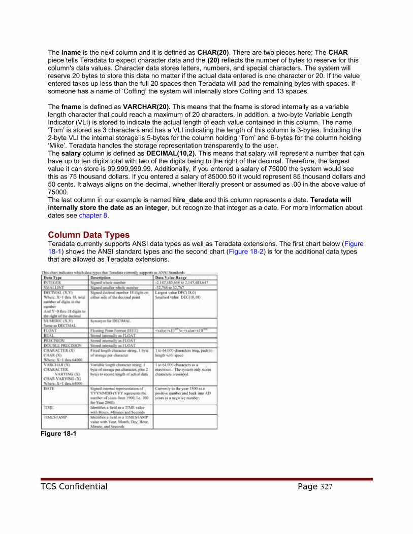
The lname is the next column and it is defined as CHAR(20). There are two pieces here; The CHAR piece tells Teradata to expect character data and the (20) reflects the number of bytes to reserve for this column's data values. Character data stores letters, numbers, and special characters. The system will reserve 20 bytes to store this data no matter if the actual data entered is one character or 20. If the value entered takes up less than the full 20 spaces then Teradata will pad the remaining bytes with spaces. If someone has a name of ‘Coffing’ the system will internally store Coffing and 13 spaces.

The fname is defined as VARCHAR(20). This means that the fname is stored internally as a variable length character that could reach a maximum of 20 characters. In addition, a two-byte Variable Length Indicator (VLI) is stored to indicate the actual length of each value contained in this column. The name ‘Tom’ is stored as 3 characters and has a VLI indicating the length of this column is 3-bytes. Including the 2-byte VLI the internal storage is 5-bytes for the column holding ‘Tom’ and 6-bytes for the column holding ‘Mike’. Teradata handles the storage representation transparently to the user.The salary column is defined as DECIMAL(10,2). This means that salary will represent a number that can have up to ten digits total with two of the digits being to the right of the decimal. Therefore, the largest value it can store is 99,999,999.99. Additionally, if you entered a salary of 75000 the system would see this as 75 thousand dollars. If you entered a salary of 85000.50 it would represent 85 thousand dollars and 50 cents. It always aligns on the decimal, whether literally present or assumed as .00 in the above value of 75000.The last column in our example is named hire_date and this column represents a date. Teradata will internally store the date as an integer, but recognize that integer as a date. For more information about dates see chapter 8.

Column Data TypesTeradata currently supports ANSI data types as well as Teradata extensions. The first chart below (Figure 18-1) shows the ANSI standard types and the second chart (Figure 18-2) is for the additional data types that are allowed as Teradata extensions.

Figure 18-1

TCS Confidential

http://www.books24x7.com/book/id_5558/viewer_r.asp?bookid=5558&chunkid=274824309#ch18fig02A6B32B41-58FA-40C7-9FE4-218ADDD95416%23ch18fig02A6B32B41-58FA-40C7-9FE4-218ADDD95416




Figure 18-2

This chart indicates which data types that Teradata currently supports as ANSI Standards:

This chart indicates which data types that Teradata currently supports as extensions:

The first example was designed to show the CREATE TABLE statement and a simple explanation of the column types. Teradata also allows you to:

Explicitly name the database where the table will reside Create the table as a SET or MULTISET table Define the protection methodologies such as FALLBACK or JOURNALING Define the internal row storage in BLOCKS and FREESPACE Further define column attributes Define CONSTRAINTS Define SECONDARY INDICES Define DEFAULT VALUES

Each will be discussed in detail.

Specifying the Database in a CREATE TABLE Statement

Someone once said, "Life is like a beautiful melody, only the lyrics are messed up". Since we did not specify a database in the previous examples, the system defaults to the current database for the CREATE TABLE statement. Sometimes this is when the lyrics get messed up. To ensure your table is placed in the intended database it is a good idea to qualify the database name in the CREATE statement.

Here is the same example again, with one change. The employee table is created in the database called TomC.

CREATE Table TomC.employee

( emp INTEGER

,dept INTEGER

,lname CHAR(20)

,fname VARCHAR(20)


,hire_date DATE )


TCS Confidential

PRIMARY INDEX considerationsOur examples have had a table level constraint of UNIQUE PRIMARY INDEX (UPI) on the column called emp. You must select a PRIMARY INDEX for a table at TABLE CREATE time or Teradata will choose one for you. There are two types of PRIMARY INDEXES. They are UNIQUE and NON-UNIQUE and are referred to as UPI and NUPI (pronounced ‘you-pea’ and ‘new-pea’). We have seen an example of a UNIQUE PRIMARY INDEX (UPI). Let us show you an example of a NON-UNIQUE PRIMARY INDEX(NUPI).


( emp INTEGER

,dept INTEGER

,lname CHAR(20)

,fname VARCHAR(20)


,hire_date DATE )

PRIMARY INDEX(dept);

Teradata also allows for multicolumn Primary Indexes, but only allow up to 16 combined columns max to represent the Primary Index. Here is an example of a multicolumn Primary Index.


( emp INTEGER

,dept INTEGER

,lname CHAR(20)

,fname VARCHAR(20)


,hire_date DATE )

PRIMARY INDEX(emp, dept, lname);

The data value stored in the column(s) of the PRIMARY INDEX (PI) is used by Teradata to spread the rows among the AMPs. The Primary Index determines which AMP stores an individual row of a table. The PI data is converted into the Row Hash using a mathematical hashing formula. The result is used as an offset into the Hash Map to determine the AMP number. Since the PI value determines how the data rows are distributed among the AMPs, requesting a row using the PI value is always the most efficient retrieval mechanism for Teradata.

If you don't specify a PI at table create time then Teradata must chose one. For instance, if the DDL is ported from another database that uses a Primary Key instead of a Primary Index, the CREATE TABLE contains a PRIMARY KEY (PK) constraint. Teradata is smart enough to know that Primary Keys must be unique and cannot be null. So, the first level of default is to use the PRIMARY KEY column(s) as a UPI. If the DDL defines no PRIMARY KEY, Teradata looks for a column defined as UNIQUE. As a second level default, Teradata uses the first column defined with a UNIQUE constraint as a UPI.

If none of the above attributes are found, Teradata uses the first column defined in the table as a NON-UNIQUE PRIMARY INDEX (NUPI).

The next CREATE TABLE statement builds a table definition for a table called employee, but does not define a Primary Index. Which column do you think it will choose?

TCS Confidential

CREATE Table employee

( emp INTEGER

,dept INTEGER

,lname CHAR(20)

,fname VARCHAR(20)


,hire_date DATE ) ;

Since there is no PI listed, Teradata must chose one. The request does not define a PK nor is there is a UNIQUE constraint. As a result, Teradata utilizes the first column (emp) as a NUPI. We suggest you always name the PI specifically in the DDL. That way there is no confusion about what column(s) are intended to be the primary index.

Table Type Specifications of SET VS MULTISET

There are two different table type philosophies so there are two different type tables. They are SET and MULTISET. It has been said, "A man with one watch knows the time, but a man with two watches is never sure". When Teradata was originally designed it did not allow duplicate rows in a table. If any row in the same table had the same values in every column Teradata would throw one of the rows out. They believed a second row was a mistake. Why would someone need two watches and why would someone need two rows exactly the same? This is SET theory and a SET table kicks out duplicate rows.

The ANSI standard believed in a different philosophy. If two rows are entered into a table that are exact duplicates then this is acceptable. If a person wants to wear two watches then they probably have a good reason. This is a MULTISET table and duplicate rows are allowed. If you do not specify SET or MULTISET, one is used as a default. Here is the issue: the default in Teradata mode is SET and the default in ANSI mode is MULTISET.

Therefore, to eliminate confusion it is important to explicitly define which one is desired. Otherwise, you must know in which mode the CREATE TABLE will execute in so that the correct type is used for each table. The implication of using a SET or MULTISET table is discussed further.

SET and MULTISET Tables

A SET table does not allow duplicate rows so Teradata checks to ensure that no two rows in a table are exactly the same. This can be a burden. One way around the duplicate row check is to have a column in the table defined as UNIQUE. This could be a Unique Primary Index (UPI), Unique Secondary Index (USI) or even a column with a UNIQUE or PRIMARY KEY constraint. Since all must be unique, a duplicate row may never exist. Therefore, the check on either the index or constraint eliminates the need for the row to be examined for uniqueness. As a result, inserting new rows can be much faster by eliminating the duplicate row check.

However, if the table is defined with a NUPI and the table uses SET as the table type, now a duplicate row check must be performed. Since SET tables do not allow duplicate rows a check must be performed every time a NUPI DUP (duplicate of an existing row NUPI value) value is inserted or updated in the table. Do not be fooled! A duplicate row check can be a very expensive operation in terms of processing time. This is because every new row inserted must be checked to see if it is a duplicate of any existing row with the same NUPI Row Hash value. The number of checks increases exponentially as each new row is added to the table.

TCS Confidential

What is the solution? There are two: either make the table a MULTISET table (only if you want duplicate rows to be possible) or define at least one column or composite columns as UNIQUE. If neither is an option then the SET table with no unique columns will work, but inserts and updates will take more time because of the mandatory duplicate row check.

Below is an example of creating a SET table:

CREATE SET Table TomC.employee

( emp INTEGER

,dept INTEGER

,lname CHAR(20)

,fname VARCHAR(20)


,hire_date DATE )


Notice the UNIQUE PRIMARY INDEX on the column emp. Because this is a SET table it is much more efficient to have at least one unique key so the duplicate row check is eliminated.

The following is an example of creating the same table as before, but this time as a MULTISET table:

CREATE MULTISET TABLE employee

( emp INTEGER

,dept INTEGER

,lname CHAR(20)

,fname VARCHAR(20)


,hire_date DATE )

PRIMARY INDEX(emp);

Notice also that the PI is now a NUPI because it does not use the word UNIQUE. This is important! As mentioned previously, if the UPI is requested, no duplicate rows can be inserted. Therefore, it acts more like a SET table. This MULTISET example allows duplicate rows. Inserts will take longer because of the mandatory duplicate row check.

Protection Features

The data warehouse of today is "mission critical" and protecting the data can become a mission. "What goes up must come down – just ask any system administrator." I was recently on a plane when I heard the words, "In case of a water landing your seat cushion will act as a floating device." Personally, this is not my idea of protection! As comedian Steven Wright once said, "Why don't they make the whole plane out of that black box stuff?" Teradata gives you a lot more assurance than a floating seat cover in shark infested waters. In fact, Teradata protects the data in numerous ways and has no single point of failure. These features are built directly into the database and can be assigned at the table level.

Attributes can be assigned within a table to provide a variety of protection features and storage characteristics. Although each of these has a default at the system level, they can be over-ridden at the time a table is created. This section discusses and demonstrates these features.

TCS Confidential

Teradata allows you to specify which data protection features to use for a table. These features include FALLBACK and Permanent Journaling. They can also be added or modified after the table has been created using the ALTER command, which is discussed later in this chapter.

FALLBACK

FALLBACK requests that a second copy of each row inserted into a table be stored on another AMP in the same cluster. This is done in case the AMP goes down or the disks fail. There are usually four AMPs grouped together in a cluster. FALLBACK allows for processing to continue in the event that an AMP is lost. As a matter of fact, FALLBACK allows for the loss of one AMP in each cluster. A cluster is normally comprised of two or four AMPs that work together.

FALLBACK provides an extra insurance policy that guarantees data availability in case an AMP is lost. However, as with all insurance policies, there is a cost. The cost for FALLBACK is that twice as much disk storage space is used for row storage as compared to not using FALLBACK. The cost is also twice the I/O on inserts, updates, and deletes because there are always two copies to write. One copy goes to the primary AMP where it belongs and the other copy goes to different AMP in the same cluster. The good news is that Teradata AMPs operate in parallel; so, it does not take twice as long to store a duplicate row. Both rows are placed on their respective AMPs at nearly the same time.

FALLBACK is an optional feature. You can use FALLBACK protection on all tables, no tables, or some tables. FALLBACK is usually created on important tables that are mission critical. Therefore, the DD is automatically FALLBACK protected. Fallback is a great feature to ensure extra protection on important data that needs to be readily available.

Here is an example of a table created with FALLBACK.

CREATE SET TABLE employee, FALLBACK

( emp INTEGER

,dept INTEGER

,lname CHAR(20)

,fname VARCHAR(20)


,hire_date DATE )


Here is another example that explicitly states NO FALLBACK

CREATE SET TABLE employee, NO FALLBACK

( emp INTEGER

,dept INTEGER

,lname CHAR(20)

,fname VARCHAR(20)


,hire_date DATE )


TCS Confidential

Teradata naturally defaults to NO FALLBACK. Because these protection features can be assigned at the database or user level it can be a good idea to explicitly state whether or not you want FALLBACK. When in doubt spell it out!

Permanent Journal

Fallback is different than the Permanent Journal. Where FALLBACK has a duplicate copy of all rows in a protected FALLBACK table, permanent journaling involves keeping an audit trail of all new, deleted or changed data. For example, if a table has one million rows and is fallback protected then there are one million fallback rows. If a Permanent Journal is used instead of FALLBACK, the only rows copied to the journal are for the inserts, updates, and deletes since the last JOURNAL backup. Therefore, in most cases this is far less expensive than storing the additional one million rows needed for fallback. Plus, you can tailor your JOURNAL with specific options. It is called a Permanent Journal because the rows stay there until the user deletes them. The user deletes them when they have been backed up to tape. This is the philosophy of the Permanent Journal.

Journal options are:

BEFORE JOURNAL - captures an image of a table row before it changes AFTER JOURNAL - captures an image of a table row after it changes DUAL BEFORE JOURNAL - captures two images of a table row before it changes and

stores the images on two different AMPs DUAL AFTER JOURNAL – captures two images of a table row after it changes and

stores the images on two different AMPs

If a table is FALLBACK protected the journal is also FALLBACK protected. However, the NO DUAL option can be added to allow the table to use FALLBACK and the journals not to utilize FALLBACK.

Besides the DUAL option on the JOURNAL table, you can also request LOCAL or NOT LOCAL. These are in reference to the AMP used in respect to the data row. LOCAL puts the journal entry on the same AMP as the data row. The default is NOT LOCAL for minimizing the loss of data relevant to the loss of an AMP.

Permanent journals are optional. They can be used for all tables, no tables, or some tables. There is one purpose for a BEFORE journal and a different purpose for an AFTER journal. The BEFORE journal is designed to perform a manual rollback in case of a programming error. An AFTER journal is designed to perform a manual roll forward in the event of a hardware failure that causes data to be lost on disk. Lets discuss both of these scenarios using two examples.

BEFORE Journal

To explain journaling, lets say that the EMPLOYEE table is created with a BEFORE journal. Then, a programmer is told to give every employee a 5% raise. Instead, every employee is accidentally given a 50% raise. Because there is a BEFORE journal you have the ability to manually rollback the data to a point in time BEFORE the employee update to correct the problem. As you can see, a BEFORE Journal might be used to rollback a programming error.

AFTER Journal

Lets look at an AFTER journal example. Lets say management has decided not to use FALLBACK on any tables. They have concluded that the data is not mission-critical and it can be restored from backup tapes in a reasonable time frame, if necessary. To make sure the system is backed up a FULL SYSTEM

TCS Confidential

BACKUP is performed on the first day of each month. Plus, an AFTER JOURNAL has been defined on all the tables in the system. Every time a new row is added or a change is made to an existing row, Teradata captures the AFTER image. Then, a hardware failure occurs on the 5th day of the month and the data is lost.

To recover, you fix the hardware problem, and then reload your data from the FULL SYSTEM BACKUP done at the 1st of the month. Then apply your AFTER JOURNAL to restore the rows that were added or changed from the 1st to the 5th day of the month. So, as illustrated here, you can use an AFTER JOURNAL to roll data forward. This is usually done to restore data lost due to a hardware problem.

The following example shows the use of the PERMANENT JOURNAL:

CREATE TABLE TomC.employee, FALLBACK

BEFORE JOURNAL,

DUAL AFTER JOURNAL

( emp INTEGER

,dept INTEGER

,lname CHAR(20)

,fname VARCHAR(20)


,hire_date DATE )


This example has created the table called employee in the TomC database. We have chosen a BEFORE JOURNAL and a DUAL AFTER JOURNAL. Journaling has a natural default of NO. That means if you don't specify this protection at either the table or database level the default is NO JOURNALING.

Knowing what you now know from the previous paragraph, how many times do you think the AFTER JOURNAL row will be stored on disk?

The answer is 4 times. This is because the table is FALLBACK protected, so the journals are also FALLBACK protected. Therefore, because the AFTER JOURNAL is DUAL each change to a row is stored twice, and two more times because both DUAL entries are also FALLBACK protected.

As you soon realize, FALLBACK with DUAL journaling can be very expensive in terms of disk space, even more so than FALLBACK by itself.

Internal Storage Options

A frustrated PC user was once quoted as saying, "Who's General Failure and why's he reading my disk?" Most people don't know what is going on inside the disks and in most cases just don't care. In a data warehouse environment having the ability to influence how data is stored inside the disks can be a great advantage. Some tables will be utilized by applications designed to read millions of records while others will operate in an OLTP type environment where updating single records is the focus.

Teradata gives the table creator the ability to influence how the data is stored on the disk. The two optional table level attributes are DATABLOCKSIZE and FREESPACE PERCENTAGE. If either of these options is not specified in the CREATE TABLE, they default to values established in the DBC Control record at the system level. Unless you are a Teradata expert let the system defaults do their job. However,

TCS Confidential

if you can understand the concepts that are about to be explained, as well as your application requirements, you can customize your disk environment to maximize effectiveness.

DATABLOCKSIZE

The DATABLOCKSIZE determines a maximum block size for multiple row storage on disk. The data block is the physical I/O unit for the Teradata file system. Larger block sizes enhance full table scan operations by retrieving more rows in a single I/O. Smaller block sizes are best for on-line transaction-oriented tables to minimize overhead by retrieving smaller blocks. You can specify this number in BYTES, KILOBYTES or KBYTES. BYTES specifications are rounded to the nearest sector of 512 BYTES. KBYTES and KILOBYTES are in set increments of 1024 BYTES.

Teradata is designed to take advantage of DATABLOCKSIZE settings because of the unpredictable nature of the data warehouse environment. While most databases ask that you define table space Teradata does not. This is because Teradata uses variable length blocks. This means that when a table is small it is allocated a few disk sectors at 512 bytes each. Then, as the table grows, the number of sectors used by the block grows with the new rows until it reaches the maximum block size. It is like a balloon. As more air is inserted, the balloon expands. Eventually the balloon gets to the maximum size and the only way to save more air is to get a second balloon.

Teradata's variable block design allows the system to handle the space instead of making the DBA do it. The DATABLOCKSIZE is the setting that determines when it is time to get additional blocks (balloons). On large data warehouse applications that read millions of rows it is best to have a few big balloons. On applications that update on one or two records at a time it is better to have many smaller balloons.

If DATABLOCKSIZE is not specified, the size used is a default of either 32256 (63 sectors) or 65024 (127 sectors), depending on the cylinder size setting. Cylinder size is a system-level value shown as SectsPerCyl with the Filer utility or Number of Disk Blocks Per Cylinder with the pdeconfig utility. Prior to V2R3.0 the default cylinder setting was 1488 sectors. With V2R3.0, the size increased the default cylinder setting to 3872 sectors.

Additionally, the block size is only the maximum when there is more than one row in a block. If a single row exceeds the DATABLOCKSIZE setting it is stored in its own data block. The block will be the length of the row and rows are never split into multiple data blocks.

MINIMUM DATABLOCKSIZE sets the minimum or smallest data block size for blocks that contain multiple rows to the minimum legal value of either 6144 or 7168 bytes (12 sectors or 14 sectors), depending on the cylinder size setting in the DBS Control Record. You can use the keywords of MINIMUM DATABLOCKSIZE or MIN DATABLOCKSIZE to change the default.

MAXIMUM DATABLOCKSIZE is the largest possible DATABLOCKSIZE setting for the table, which is 65024 bytes (127 sectors). You can use the keywords MAXIMUM DATABLOCKSIZE or MAX DATABLOCKSIZE to change the default.

Normally, larger block sizes require less physical disk space. This is because large blocks contain more rows. Therefore, fewer blocks are needed and since each block requires a block header and control data, less space needs to be allocated for them.

FREESPACE PERCENTAGE

The FREESPACE PERCENTAGE tells the system at what percentage Teradata should keep a cylinder free of rows on data loads when using Fastload and Multiload load utilities. A FREESPACE 10 PERCENT keeps 10% of a cylinder's sector space free when loading the data. Valid values for the percentage of free space range from 0-75.

TCS Confidential

The value used for FREESPACE should mimic the usage of the table. As the number of rows being inserted by clients, other than Fastload and Multiload increases, the value of FREESPACE might also increase. This causes the secondary row inserts to execute faster because space is already available on disk to store the new rows in the same cylinder. Therefore, fewer cylinder splits will occur as a result of insufficient space at insert time. In other words, we don't blow the "balloon" all the way up. We know we will be utilizing SQL to do more inserts and we want extra room for the balloon to expand.

On the other hand, if the tables only receive rows loaded by Fastload and Multiload, the FREESPACE value can be set to 0 for maximum utilization of the disk space within each cylinder since inserts are not performed by other clients. If we are not going to use SQL commands to insert additional data we can blow the balloon all the way up because it won't need to expand any further.

Since these parameters have defaults kept in system parameters as part of the DBS Control record, they are seldom used in the CREATE TABLE statement, but Teradata gives you the option of over-riding the default on any particular table.

The following CREATE TABLE specifies FALLBACK and establishes values for both DATABLOCKSIZE and FREESPACE:

CREATE Table TomC.employee, FALLBACK,

DATABLOCKSIZE=16384 BYTES,

FREESPACE = 20 PERCENT

(

emp INTEGER

,dept INTEGER

,lname CHAR(20)

,fname VARCHAR(20)


,hire_date DATE

)


As previously mentioned, if you don't specify a DATABLOCKSIZE or FREESPACE PERCENT then the system builds the table using the default parameters for DATABLOCKSIZE and FREESPACE PERCENT found in the DBS Control Record. Never specify these without a discussion with your database administrator. Remember, to change and to change for the better are two different things. If you don't know it – don't blow it!

Column Attributes

Alfred North Whitehead once said, "We think in generalities, but we live in details". We have seen examples in this chapter of creating tables with simple column definitions. These examples have been generalities, but often we need to model our columns in great detail. It is time to take the next step. When defining a table it is normally advantageous to be more specific regarding the definition of the columns and their attributes.

TCS Confidential

Figure 18-3

The next CREATE TABLE builds a table definition with attributes.


(

emp INTEGER

,dept INTEGER NOT NULL

,lname CHAR(20) NOT CASESPECIFIC

,fname VARCHAR(20) TITLE 'FIRST NAME'

,salary DECIMAL(10,2) FORMAT 'ZZ,ZZZ,ZZ9.99'

,hire_date DATE FORMAT 'mmmBdd,Byyyy'

,Byte_col BYTE(10) compress '000000'xb

) UNIQUE PRIMARY INDEX(emp);

In the above example the columns have been further defined using column attributes. The dept column is defined with the NOT NULL attribute. This means that a NULL value cannot be stored in the dept column.

The lname column has been further defined to state that for comparison purposes, the data is not casespecific. This means that it does not matter if the data is in upper case, lower case, or a combination.

The fname column has a TITLE associated with it. So, whenever it is selected, ‘FIRST NAME’ appears as the report heading instead of the column name.The salary column is automatically formatted as currency in the output when selected using BTEQ.

The hire_date is also formatted. It displays as the alpha month followed by the numeric day and 4-digit year.

Lastly, the Byte_Col column is added. It is a byte column with a length of 10. The example shows how to initialize it with a value of zero. It is provided as a hexadecimal number using the xb designation. This designation would also be a valid comparison for retrieval of the row. Notice the word compress.

This compress does not mean we are going to use WINZIP to shrink the column. Compress allows you to take one specific value and store the default in the table header. Let me explain. Lets say the Dept of Motor Vehicles in California has a database that tracks all people with a California driver's license. Around 99.9% of the drivers would have California as their state code on their address. Instead of storing "CALIFORNIA" in millions of records the compress will store the value "CALIFORNIA" in the table header. Now, a value can be assumed in a row as a default unless another value exists inside the column.

TCS Confidential

Constraints

One of our best Teradata training customers has a data warehouse with over 40,000 users. Even though their enterprise data warehouse may span continents, the data warehouse Return On Investment game is played on a field that is 5 inches wide. The space between the users ears! It is the users that make the data warehouse great. When users gain experience and use intuition, imagination, and experience they can find the company big dollars. When Users can ask any question, at any time, on any data, the boundaries are unlimited.

But sometimes boundaries are necessary! At times it is advisable to add restrictions to the table and columns within a table. This is done to provide data integrity, availability and ease of use to the table and its data. Users can still use their imagination and ask any question, but on all inserts, updates, and deletes Teradata will be watching.

Relational theory describes columns and the attributes a column can have as part of a domain. The domain includes the data type and valid value boundaries based on business requirements or restrictions. Because ANSI does not support a rigorous atomic definition of a domain, it is up to the database designer to define the domains for a table and their legal values by creating constraints on one or more columns. Constraints keep the table in check to enforce certain rules.

Think of domains as standards. If everyone in the company tracking information about employees sets up the employee number as an integer ranging from 1 – 100,000,000 then when there is cross functional analysis across business units each will see employee number as an integer. Comparisons will be easy. Make columns with the same functions the exact same data types (with the same range) and your columns are said to be from the same domain.

Teradata has some fundamental rules about constraints:

Always name table level constraintsConstraint names can be up to 30 charactersConstraint names must be unique among all other constraint names defined for a tableConstraints can be specified at the column or table levelThe system does not assign names to constraints you do not name

You also have the ability to define constraints on column values during the CREATE Table process. This can also be done using the ALTER command once the table has been created. Constraints generally fall into three areas:

UniqueCheckReferential Integrity

Constraints are defined at the column or table level.

TCS Confidential

Figure 18-4

Figure 18-5

UNIQUE Constraint

The great writer Mark Twain was quoted as saying, "Whenever you find you are on the side of the majority, it is time to pause and reflect." Sometimes it is good to be on the side of the majority, but at other times it is best to be UNIQUE. The UNIQUE constraint is used to enforce uniqueness of values stored within the column(s). This means that no two rows in the table can have the same value for the column or columns utilizing the UNIQUE constraint.

An employee number is an excellent example. Each employee must have an employee number, and no two employees can ever have the same employee number. At the same time, we must ensure that no employee has NULL data for their employee number. The Teradata system enforces the uniqueness by making a column with the UNIQUE constraint a Unique Secondary Index (USI). Teradata makes the column a Unique Primary Index (UPI) only if during the TABLE CREATE statement no Primary Index or PRIMARY KEY is explicitly stated.

When a table is created using this constraint, rows containing duplicate values cannot be stored in the table. If the table is not created using a UNIQUE constraint and it is later altered to add the constraint, if the data is not unique the ALTER statement fails because the data violates the constraint.

CHECK Constraint

Even Wayne Gretzky, the greatest hockey player ever missed a check on occasion, but Teradata will not! The CHECK constraint allows for a range of values to be checked or for specific value limits to be placed on a column. For example you can check that a column value falls within a certain range such as EMP BETWEEN 1 AND 99. You can also check to see that a column value is greater than another column or value. As an example: CHECK EMP > 0. You can also CHECK EMP > DEPT. You can even utilize a compound check like EMP BETWEEN 1 AND 99 AND EMP > DEPT.

When a table is created using this constraint, rows containing invalid values cannot be entered into the table. If the table is altered later on with a CHECK, and the data is not valid for the constraint, the ALTER statement fails since the data violates the constraint.

TCS Confidential

Referential Integrity (RI) Constraint

Referential Integrity (RI) insists that a row cannot be inserted unless the value in the column has a corresponding value existing in another table. This also means a row cannot be deleted if a corresponding value in another table still exists. For example, imagine getting fired and your employer deletes you from the employee table, but forgets to delete you from the payroll table. A RI check can be used to enforce data integrity and prevent this scenario. Referential Integrity does not allow anyone to be deleted from the employee table unless they were already deleted from the payroll table. Darn, RI can hurt your Bahamas retirement.

When RI is established on a new table, invalid data values cannot be entered into a column. However, if a table is altered to begin enforcing RI, the data might already be incorrect. When this happens, the ALTER creates a copy of the original table and stores rows in it that violate the RI constraint. It is up to you to look for the table copy and correct any errors in the actual table. RI is the only constraint that can be added with data that violates the constraint.

Defining Constraints at the Column level

It is possible to establish the constraint directly on the column definition. It makes for an easy definition process. However, it does spread the varying constraints throughout the DDL statement. Sometimes the CREATE TABLE can be very large! This makes the constraints a bit more difficult for people to find. We have seen constraints placed at the column level on DDL so large that Magellan couldn't find his way through it.

The other issue for a column level definition is that only one column can be involved. Since some constraints may involve multiple columns, these definitions must be defined at the table level and not the column level. Both levels are covered in this section.

Here is an example of creating a table with column level constraints:


( emp INTEGER NOT NULL

CONSTRAINT EmpPK PRIMARY KEY

,dept INTEGER CONSTRAINT Ref_1 REFERENCES Department(dept)

BETWEEN 10 AND 100

,lname CHAR(20) NOT NULL

,fname VARCHAR(20) NOT NULL

,salary DECIMAL(10,2) CONSTRAINT SalCheck

CHECK (salary >=10000 and salary < 1000000)

,hire_date DATE

,soc_sec INTEGER NOT NULL

CONSTRAINT NameUniq UNIQUE ) ;

In the above table, the emp column must have a value because it cannot be null. It also has a primary key named EmpPK and therefore, becomes the UPI of this table because no Primary Index was explicitly defined.

The dept column has an RI constraint named Ref_1 on the column called dept in the Department table. This means that a dept cannot be entered into the employee table unless that dept exists in the department table. This is referential integrity as its best!

TCS Confidential

There is a CHECK constraint called SalCheck on the salary column and it requires the salary to be at least $10,000.00 up to a maximum of $99,999.99.The last two constraints are on the soc_sec column. First, there is the NOT NULL that requires a value to be stored there. Then, the NameUniq constraint requires that the value be different from any other value in other rows because it must be unique.

Defining Constraints at the Table Level

Besides using column level constraints, table level constraints can also be used. This is the only way to implement multi-column constraints. A multi-column constraint involves more than one column. All table level constraints should always be named. Table level constraints are established after the column definitions. Here is an example:

CREATE Table TomC.employee, FALLBACK

( emp INTEGER NOT NULL

,dept INTEGER

,lname CHAR(20) NOT NULL

,fname VARCHAR(20) NOT NULL

,sal DECIMAL(10,2)

,hire_date DATE

,soc_sec INTEGER NOT NULL,

CONSTRAINT EmpPK PRIMARY KEY (emp),

CONSTRAINT Ref_1 FOREIGN KEY (dept) REFERENCES Department(dept),

CONSTRAINT NameUniq UNIQUE (lname, fname),

CONSTRAINT Sal_Dept_Check CHECK (sal >= 10000 AND sal < 100000

AND dept BETWEEN 10 AND 100),

CONSTRAINT NameUniq UNIQUE (soc_sec) ) ;We feel this type of definition is easier to read and understand than looking for constraints throughout the DDL. These constraints are all the same as in the first example, with one exception. Here, the name constraint called NameUniq uses a combination of both the fname and the lname columns to create a USI. Notice too that NOT NULL must still be at the column level.

Utilizing Default Values for a Table

A default value control phrase determines the action to be taken when you do not supply a value for a field. Default value control phrases are only valid when used with the columns defined in the CREATE TABLE and ALTER TABLE statements as well as parameters defined in the CREATE MACRO and REPLACE MACRO statement.

A default value control phrase determines the action to be taken when you do not supply a value for a field. Instead of placing a NULL the system will place the default value listed in the CREATE or ALTER table command. The following rules and guidelines apply to default value control phrases:

Fields must be defined in CREATE TABLE and ALTER TABLE statementsParameters must be defined in CREATE MACRO and REPLACE MACRO statements

TCS Confidential

Default value controls are not effective for views and expressions.The normal default value for a field is null unless you specify NOT NULL.

Teradata allows you to specify default values when creating a table. As seen earlier, the keyword DEFAULT VALUES can be used in an INSERT. When this is done, any columns that have default values defined in the CREATE TABLE statement use the default instead of a NULL. All columns without a DEFAULT phrase defined for them contain a NULL. However, if a column does not have a DEFAULT defined and has an attribute of NOT NULL, an error is returned and the insert fails.

Below is an example of a table with defaults.

CREATE TABLE TomC.Dept_Defaults

( Dept INTEGER DEFAULT 10

,Dept_name CHAR(20) DEFAULT 'Sales'

,Mgr_Emp# INTEGER

)

PRIMARY INDEX(dept);

We have now created an empty table called Dept_Defaults. We will now insert data in our next example.

INSERT INTO TOMC.DEPT_DEFAULTS DEFAULT VALUES;

We will now select from the DEPT_DEFAULTS table.

SELECT * from TOMC. DEPT_DEFAULTS;

1 Row Returned

Dept Dept_name Mgr_Emp#

10 Sales ?

CREATE TABLE to Copy an existing table

Confucius taught us "A journey of a thousand miles begins with a single step." The journey of the DBA copying a table used to be inefficient and contain too many steps. Teradata V2R4, has taken on the challenge, stepped up to the plate and scored a home run. In Teradata V2R4 and beyond, there is a new format that does it all in one easy command.

It has been modified to create a new table from the definition of an existing table. The only difference between the tables is the table-name. All columns have the same names, data types and constraints. All indices and table options are also identical.

The new syntax is:

CREATE TABLE [<database-name>.]<table-name> AS

[<database-name>.]<original-table-name>

WITH { DATA | NO DATA }

[ [ UNIQUE ] PRIMARY INDEX (<column-list>) ]

;

Notice the specification of WITH. It is required and requests either the DATA or NO DATA specification. When DATA is requested, not only does the system create the new table, but it also copies all of the rows

TCS Confidential

and columns from the original table into the new table. The NO DATA specification means that the original data rows are not to be copied into the new table. It remains empty of rows.

This is nice because it is now easier than using the SHOW TABLE to get the DDL, copying the DDL, changing the table-name and then submitting the DDL. Plus, if you do want the data rows, there is no need to perform a separate INSERT/SELECT. Optionally, another database or user area may be used to qualify the names of the two tables. Creating and duplicating tables has never been easier! In addition, the "existing" table could be a derived table, but you probably want to specify which column or columns to use as the primary index.

Altering a Table

The only thing in life we can consistently count on is change. This is especially true in a data warehouse environment. As business requirements change, sometimes it is necessary to reflect those changes into the tables. Teradata allows for modification of a table at either the table or column level using the ALTER command.

Here is a list of the table changes available to the ALTER TABLE:

Add one or more new columns to an existing table.Add new attributes for one or more columns in a table. Drop one or more new columns to an existing table.Modify constraints on an existing table at the column or table level.Add or remove FALLBACK or JOURNALINGModify the DATABLOCKSIZE or FREESPACE PERCENTChange the name of a column in an existing table

You can ALTER a TABLE at both the column and table level. A table level change includes protection features or internal storage options such as FALLBACK, JOURNALING, FREESPACE PERCENT, etc. The column level allows you to change individual column attributes. For example you might be adding the TITLE, FORMAT, or another column level change.

The syntax for the ALTER statement is:

ALTER TABLE [<database-name>.]<table-name>



[ ADD <column-name> [ <data-type> ] [ <attribute-list> ] ]

[ DROP <column-name>]

[ ADD <table-level-constraint> ]

[ MODIFY <table-level-constraint> ]

[ DROP <table-level-constraint> ]

;

The following ALTER modifies the table to FALLBACK at the table level:

ALTER TABLE TomC.Employee, FALLBACK;

The Employee table in the TomC database now has a FALLBACK copy of each row. You can also remove FALLBACK, which is quick and easy. The system merely places the FALLBACK blocks of a table on the Free Cylinder List and the blocks are gone. This happens immediately. However, adding FALLBACK to a

TCS Confidential

table is another story. This change may take a lot of time, depending on the number of rows in a table. When you add FALLBACK the system duplicates each row and places that row on another AMP in the same cluster. You are essentially doing a Full Table Scan (FTS) and a copy. If you have a million rows in the base table you are creating and distributing a million FALLBACK rows. The good news is that Teradata does this in parallel!

The following ALTER makes journaling changes at the table level:

ALTER TABLE TomC.Employee, NO BEFORE JOURNAL, DUAL AFTER JOURNAL;

The Employee table no longer has a BEFORE JOUNAL and now has a DUAL AFTER JOURNAL.

The following ALTER adds a TITLE of ‘School’ to one of the existing columns:

ALTER TABLE TomC.School

ADD School_Name TITLE 'School';

Although the above appears to be adding a column, the School_Name column already exists. When we explained Teradata to Sherlock Holmes he found another clue. Sherlock said, "Since the School_Name did not contain a data type, it could not possibly be adding a new column, but could only be altering an existing column." Sherlock was impressive. I went on to ask him what type of school he thought this table held. He said, "Elementary my dear".

You can make multiple changes to a table with one ALTER statement. The next request makes multiple changes to a table by adding multiple columns.

This example adds FALLBACK and two new columns (Soc_Sec and Dept_Name) to the table Employee:

ALTER TABLE TomC.Employee, FALLBACK

ADD Soc_Sec INTEGER

,ADD Dept_Name Char(20);

Notice in the above example that when adding new columns you must specify a data type.

The next request makes three changes to the table. The first is a journaling change at the table level. The second is at the column level and it drops the column called Soc_Sec. The third change is also at the column level. It adds a TITLE to the column called Dept_Name:

ALTER TABLE TomC.Employee, DUAL AFTER JOURNAL

DROP Soc_Sec,

ADD Dept_Name TITLE 'Dname';

The next request changes the name of a column. The old column name was lname and the new column name is Last_Name.

ALTER TABLE TomC.Employee

Rename lname to Last_Name;

There are some restrictions when renaming columns, they are:

A new column name cannot match any existing column name in the same tableThe affected column cannot be a part of an indexThe affected column cannot be part of a referential integrity constraintThe affected column cannot be referenced in the UPDATE OF clause of a trigger

TCS Confidential

Dropping a Table

The opposite of the CREATE TABLE command is the DROP TABLE. The DROP command deletes objects out of the Data Dictionary (DD) and the data rows inside the table are deleted from the system. Be CAREFUL! Gone is gone. So, make sure you are in the correct database!

The syntax to drop a table is:

DROP TABLE [<data-base-name>.]<table-name>

;

To ensure you are dropping the correct table you can also specify the database where the table resides by qualifying the table name with the database name.

To drop the table Employee in the database TomC you can use this command:

DROP TABLE TomC.Employee;

You can use two different SQL commands to accomplish the same thing. The first switches to the database TomC And the second drops the table.

DATABASE TomC;

DROP TABLE Employee;

Because you can have the same table names in different databases it is important when performing the DROP function that you are sure you are getting rid of the table you want to drop.

Dropping a Table versus Deleting Rows

In most database systems, it is faster to drop a table than it is to delete of the rows. It is exactly the opposite in Teradata. As mentioned earlier, the delete of all rows of a table is the fastest thing that Teradata does. So, if you wish to get rid of all of the rows, use the DELETE command instead of the DROP command.

Furthermore, once a table is dropped it is no longer in the system. The data definition stored in the DD is gone. The access rights to the table are also deleted from the access rights table. There are times when a database administrator or user drops a table and creates the table again to fill it with fresh data. When doing this, the access rights of previous users need to be re-established.

This is why you drop a table when it is no longer needed, but DELETE the data rows from a table that you want to refresh with new data. A table loaded monthly with new data might fit this category. This allows the access rights to remain the same. The old data is deleted and the new data loaded. The access rights are unaffected because the data definition in the DD has not changed and the access rights table is not affected.Additionally, since the DROP requires locking the DD for WRITE to drop the table and delete the rows, a DELETE for just the data rows is faster. A DELETE of rows within a table is fast. It is much faster than a DROP because a DROP is actually deleting multiple rows from multiple DD tables. For more details on the speed of a DELETE command, see chapter 13 in this book.

Renaming a Table

The next capability discussed here is the ability to rename an existing table. The RENAME TABLE command is useful when a table name needs to be changed.

The syntax of the RENAME command:

TCS Confidential


RENAME TABLE [database-name>.]<table-name>

TO [database-name>.]<table-name>

;

Here is an example:

RENAME TABLE TomC.Employee to TomC.EmpXX;

We have changed the table named Employee to EmpXX.

Using Secondary Indices

The Primary index is always done at table create time. The Primary Index is the mechanism used to distribute the table rows evenly across the AMPs. Every table in Teradata must have one and only one Primary Index and it is the fastest way to retrieve data. A table can also have up to 32 secondary indices. All indices can be single column or multiple columns. A multi-column secondary index can be any combination of up to sixteen columns.

A secondary index becomes an alternate read path to the data. They can be an excellent way to speed up queries. A secondary index can be defined as a Unique Secondary Index (USI) or Non-Unique Secondary Index (NUSI).

The following is the syntax for creating a secondary index:

CREATE [UNIQUE] <index-name> (<column-list>)

[ORDER BY VALUES [ (<column-list>) ] ] on [database.]<table-name>

[ALL]

;

The example below does not specify UNIQUE and therefore creates a non-unique secondary index on the dept column of the table Employee.

CREATE INDEX(dept) on TomC.Employee;

The next example creates a unique secondary index(USI) on the combination of first and last names with an index name of name_idx_1in the Employee table.

CREATE UNIQUE INDEX name_idx_1 (fname, lname) on TomC.Employee;

Why would someone choose to name an index? It is easier to drop if it is a multi-column index. You would just use the syntax:

DROP INDEX name_idx_1 on TomC.Employee

The next example creates a Non-unique secondary index (NUSI) on the last name and assigns a name of name_idx_2 for it:

CREATE INDEX name_idx_2 (lname) on TomC.Employee;

When initially creating an USI, the rows of the table must all be read using a full table scan. During this process, if a duplicate value is encountered, the CREATE INDEX command fails. All duplicate values must be eliminated before an USI can be created.

The table Employee now has three secondary indices. A non-unique index on the column dept, a unique index on the fname and lname combination, and a non-unique index that is named name_idx on lname.

TCS Confidential

Remember, we suggest that you name any index that uses more than one column. If you wish to name an index with one column, the suggestion is to use a name that is shorter than the column name.

You can also drop an index that is not named. The following drops the index on a multi-column key in the Employee table:

Drop index (lname,fname) on TomC.Employee;

A classical secondary index is itself a table made up of rows having two main parts. The first is the data column itself inside the secondary index table, and the second part is a pointer showing the locations of the row in the base table. Because Teradata is a parallel architecture, it requires a different means for distributing and retrieving its data – hashing.

Teradata has a very clever way of utilizing unique secondary indices. When a secondary index command is entered Teradata hashes the secondary index column value for each row and place the hash in a secondary index subtable along with the ROW-ID that points the base row where the desired value resides. This approach allows for all USI requests in the WHERE clause of SQL to become two-AMP operations. A NUSI used in the WHERE clause still requires all AMPs, but the AMPs can easily check the secondary index subtable to see if they have one or more qualifying rows.

Teradata creates a different secondary index subtable for each secondary index placed on a table. The price you pay is disk space and overhead. The disk space comes from PERM for the secondary index subtables and there is overhead associated with keeping them current when a data row is changed or inserted. There are three values stored in every secondary index subtable row. They are:

Secondary Index data valueSecondary Index Row-ID (This is the hashed version of the value)Primary Index Row-ID (This locates the AMP and the row of the base row)

Hashing the secondary index value and storing it in the secondary subtable is a fast and efficient way to gain an alternate path to the data. This is extremely efficient unless the query asks for a range of values to be selected. For example, many queries involving dates ask for a range based on a start and end date using the WHERE clause. The query might try to find all orders where the order_date is between December 25, 2001 and December 31, 2001. A secondary index done on a DATE field does not allow for a range unless it is VALUE-ORDERED instead of HASH-ORDERED.

We suggest that all DATE columns, where you want a secondary index for range queries, should specify the secondary indices to be VALUE-ORDERED. A value ordered NUSI stores the subtable rows in sequence by the data value and not by the row hash value. Therefore, range checks work very well. The golden rule for Value-Ordered secondary indices is that they can only be performed on a single column NUSI that is four-bytes or less. Valid data types supported are:

DATEBYTEINT INTEGERDECIMALSMALLINT

Here is an example of creating a value-ordered secondary index on Hire_date.

CREATE INDEX (Hire_date) ORDER BY VALUES on TomC.Employee ;

There is no such thing as a value ordered USI. So, do not use the UNIQUE keyword when attempting to create this type of index. There are only Value-Ordered NUSI's.

TCS Confidential

If statistics are not collected for a NUSI column (see next section in this chapter for COLLECT STATISTICS), the optimizer will never use the NUSI when referenced in a WHERE clause. Also, a composite NUSI (multi-column) will almost never be used, even with statistics. Instead, it is usually better to make multiple NUSI indices and collect statistics on all of them. This allows Teradata to use what is called Bitmap Set Manipulation (BMSMS in the EXPLAIN output). This uses the selectivity of multiple NUSIs together to make them highly selective and therefore used for row retrieval. .

Join Index


A Join Index is an index table that pre-joins the joined rows of two or more tables and, optionally, aggregates selected columns. They are used to speed up queries that frequently join certain tables. Teradata join indexes can be defined as hash-ordered or value-ordered. Join indexes are defined in a way that allows join queries to be resolved without accessing or joining their underlying base tables.A Join Index takes two or more tables and physically joins the tables together into another physical index table. It also updates the Join Index table when the base rows of the joining base tables are updated. Join indexes are a great way to aggregate columns from tables with a large range of values. A Join Index can play the role of a summary table without denormalizing the logical design of the database and without causing update anomalies presented by denormalized tables. This actually gives you the ability to keep your detail data in 3rd normal form and your summary tables in a star schema format. Brilliant Teradata!

The syntax for a JOIN INDEX is:

CREATE JOIN INDEX [<database-name>.]<index-name>

[[NO] FALLBACK]

AS SELECT

[<columns>]

[SUM numeric-expression]

[COUNT column-expression]

[EXTRACT year | month from date-expression]

FROM [<database-name(s)>.]<table-names>]

[WHERE <search-condition>]

[GROUP BY <column-name>]

[ORDER BY <column-name>]

PRIMARY INDEX(<column-name>)

[index <column-name> ORDER by HASH | VALUES]

;

Here is an example of creating a Join Index between the Employee table and the Department table:

CREATE JOIN INDEX TOMC.emp_dept_idx AS

SELECT emp, e.dept, lname, fname, sal,

TCS Confidential


dname, mgremp, budget

FROM TomC.Employee as e INNER TomC.Department as d

ON e.dept = d.dept;In the example above a JOIN INDEX called emp_dept_idx has been created on the tables Employee and Department. The rows from the two tables have been physically joined together and will be maintained when rows in the Employee or Department tables change because of INSERTS, UDATES, or DELETES. When users run queries they don't specify or mention the JOIN INDEX table. Instead, when they run queries that can be satisfied by the JOIN INDEX table faster the Teradata database will choose to pull the data from the JOIN INDEX table instead of the base tables. When SQL is run and the columns asked for are any combination of the above columns defined in the JOIN INDEX then Teradata may choose to use the JOIN INDEX instead of the actual base tables. This is called a covering query.

You can also explicitly define a Primary Index for a JOIN INDEX. Teradata spreads the rows of the join index across the AMPs. The AMPs read and write the rows in parallel. So, utilizing a good Primary Index can be important.

CREATE JOIN INDEX TOMC.JOINIDX_2 AS

SELECT emp, e.dept, dname

FROM TomC.Employee as e, TomC.Department as d

WHERE e.dept = d.dept

PRIMARY INDEX(emp);

You can also drop a JOIN INDEX. Here is an example:

DROP JOIN INDEX TOMC.JOINIDX_2;

Collecting Statistics

The Teradata PE or optimizer follows the saying, "If you fail to PLAN you PLAN to fail". The PE is responsible for taking users SQL and after optimizing the SQL comes up with a PLAN for the AMPs to follow. The PE is the Boss and the AMPs are the workers. Ask yourself two questions:

1. Could you have a Teradata system without AMPs? Of course not! AMPs read and write the data.

2. Could you have a Teradata system without PE's? Of course not! Could you get along without your boss? (kidding, kidding)

The Teradata Parsing Engine (PE) is the best optimizer in the data warehouse world, but it needs you to COLLECT STATISTICS so it can optimize its work. The statistics allow the optimizer to use its vast experience to PLAN the best way to fulfill the query request. It is particularly important for the optimizer to have accurate table demographics when data is skewed.

The purpose of the COLLECT STATISTICS command is to gather and store demographic data for one or more columns or indices of a table or join index. This process computes a statistical profile of the collected data, and stores the synopsis in the Data Dictionary (DD) for use during the PE's optimizing phase of SQL statement parsing. The optimizer uses this synopsis data to generate efficient table access and join plans.

Lets review: The Parsing Engine Processor (PEP) which is also referred to as the optimizer takes SQL requests from a user and comes up with a Plan for the Access Module Processors

TCS Confidential

(AMPs) to execute. The PEP uses statistics to come up with the most cost efficient plan. You must COLLECT STATISTICS on any columns or indices of a table you want the optimizer to use with high confidence.

If statistics are not collected, the PE randomly chooses an AMP in which it will ask a series of questions. The PEP will then estimate based on the total number of AMPs to estimate the number of rows in the entire table. This "guess-timate" value can be inaccurate, especially if the data is skewed.You should COLLECT STATISTICS on all tables. You also have the ability to COLLECT STATISTICS on a Global temporary tables, but not Volatile tables.

We recommend you refresh the statistics whenever the number of rows in a table is changed by 10%. For example, a MultiLoad job may INSERT a million records in a 9 million-row table. Since the table has an additional 10% of new rows it is definitely time to refresh the COLLECT STATISTICS. In reality, we refresh statistics by using the COLLECT STATISTICS command again any time the table changes by more than 10%.

The first time you collect statistics you collect them at the index or column level. After that you just collect statistics at the table level and all previous columns collected previously are collected again. It is a mistake to collect statistics only once and then never do it again. In reality, it is better to have no statistics than to have ridiculously incorrect statistics. This is because the optimizer is gullible and believes the statistics, no matter how inaccurate.

Collecting Statistics is rough on system resources so it is best to do it at night in a batch job or during other off peak times. You can see what statistics have been collected on a table and the date and time the STATISTICS were last collected with the following:

HELP STATISTICS <table-name> command

;

Here are some excellent guidelines on what you should collect statistics on:

All Non-Unique indicesNon-index join columnsThe Primary Index of small tablesPrimary Index of a Join IndexSecondary Indices defined on any join indexJoin index columns that frequently appear on any additional join index columns that

frequently appear in WHERE search conditionsColumns that frequently appear in WHERE search conditions or in the WHERE clause of

joins.

The two key words to collect and drop statistics are:

COLLECT STATISTICS DROP STATISTICS

Here is the syntax to collect statistics:

COLLECT STATISTICS ON <table-name>

[COLUMN <column-name> | INDEX(<column-name>) ]

;

TCS Confidential

Here is an example of collecting statistics on the column dept and the multicolumn index of lname, fname columns in the employee table.

COLLECT STATISTICS on TomC.Employee column dept;

COLLECT STATISTICS on TomC.Employee Index(lname, fname);We have COLLECTED STATISTICS for the employee table in two separate statements. You will always COLLECT STATISTICS on a column or index one at a time initially. You must use the COLLECT STATISTICS command for each column or index you want to collect in a table. In the above examples, we collected statistics on the column dept and the index(lname, fname). You can collect statistics at either the column or index level. It is best to COLLECT STATISTICS at the column level unless you are dealing with a multi-column index. COLLECT at the index level only for indices that are multicolumn indices. Otherwise collect columns and single column indices at the column level. Single column indices actually perform the same COLLECT STATISTICS functions as if they were collected at the column level. Plus, if you drop an index, you lose the statistics.

The table Employee now has COLLECTED STATISTICS defined within the table. Although you must collect statistics the first time at the column or index level you only collect statistics at the TABLE LEVEL for all refreshing of STATISTICS. Here is an example of COLLECTING STATISTICS at the table level.

COLLECT STATISTICS on TomC.Employee;

The system will refresh the COLLECT STATISTICS on the columns and indices it had previously collected on the table.

Hashing Functions

Teradata uses parallel processing with its architecture of AMPs and PEPs. The Primary Index must be chosen whenever you create a table because it is the sole determinant of which AMPs owns which rows. This concept pertains to data storage and data retrieval. Picking the proper column(s) for the Primary Index is extremely important for distribution and therefore, for performance. The hashing functions introduced in this section provide information pertaining to the selection of the AMP where each individual row is stored.

As mentioned previously, Teradata uses a hashing algorithm to determine which AMP is responsible for a data row's storage and retrieval. This mathematical meat grinder is configured to generate a 32-bit binary number called the Row Hash for any data value passed to it. This makes the placement of rows on AMPs a random process. Yet, it will generate the same 32-bit value whenever the same data value is passed into it. Then, the first 16-bits called the Destination Selection Word (DSW) is used to select the appropriate AMP. Using this technique over a large number of rows with unique values, the system normally generates a good distribution of data rows the vast majority of the time.

There are now hashing functions, which can be incorporated into SQL, to produce and use the same hash value result for testing current or future distribution levels. In other words, these functions can be used to evaluate the distribution of the rows within any or all tables or determine the acceptability of other columns as a potential primary index.

HASHROW

The HASHROW function is used to produce the 32-bit binary (BYTE(4) data type) Row Hash that is stored as part of the data row. It can return a maximum of 4,294,967,295 unique values. The values produced range from 0 to FFFFFFFF.

TCS Confidential

One might think that 16 different values can be passed to the HASHROW function since 16 columns can be used in an index. However, we have used up to 50 different values and it continues to produce unique output values.

The basic syntax for using the HASHROW function follows:

SELECT HASHROW( [ <data-column-value> [, <data-column-value2> ... ] ] )

;

Examples using HASHROW:

SELECT HASHROW(NULL) AS NULL_HASH

,HASHROW('Larkins') AS Lark_HASH

,HASHROW() AS NO_HASH ;

1 Row Returned

NULL_HASH Lark_HASH NO_HASH

00000000 E4E7A3BC FFFFFFFF

Now that the functionality has been demonstrated, a more realistic use might be the following to examine the data distribution and determine the average number of rows per value:

SELECT COUNT(*) / COUNT(DISTINCT(HASHROW(Student_id)))

AS AVG_ROW_CT

FROM Student_table;

1 Row Returned

AVG_ROW_CT

1

As good as this is, the HASHROW function does not provide a lot more help in the evaluation process. However, when combined with the other Hashing Functions, it yields some very helpful data demographics.

HASHBUCKET

The HASHBUCKET function is used to produce the 16-bit binary Hash Bucket (the DSW) that is used with the Hash Map to determine the AMP that should store and retrieve the data row. It can return a maximum of 65,536 unique values. The values range from 0 to 65535, not counting the NULL as a potential result. The input to the HASHBUCKET is the 32-bit Row Hash value.

The basic syntax for using the HASHBUCKET function follows:

SELECT HASHBUCKET( [ <row-hash-value> ] )

;

Example using HASHBUCKET function:

SELECT HASHBUCKET(NULL) AS NULL_BUCKET

,HASHBUCKET() AS NO_BUCKET;

TCS Confidential

1 Row Returned

NULL_BUCKET NO_HASH

? 65535

A more realistic use is to determine the number of rows in each Hash Bucket using the following SELECT:

SELECT COUNT(*) AS NBR_ROWS

,HASHBUCKET(HASHROW (Student_ID)) AS Bucket_No

FROM Student_table

GROUP BY 2 ;

10 Rows Returned

NBR_ROWS Bucket_No

1 1056

1 26871

1 9645

1 11534

1 22451

1 47645

1 59094

1 22211

1 40241

1 30439

The Hash Bucket is also known as the Destination Selection Word (DSW). This is due to its use of the Hash Bucket to determine the destination AMP. Like Teradata, the SELECT can use the HASHBUCKET as input into the HASHAMP function.

HASHAMP

The HASHAMP function returns the identification number of the primary AMP for any Hash Bucket number.

The input to the HASHAMP function is an integer value in the range of 0 to 65535. When no value is passed to the HASHAMP function, it returns a number that is one less than the number of AMPs in the current system configuration. If any other data type is passed to it, a run-time error occurs.

The basic syntax for using the HASHAMP function follows:

SELECT HASHAMP( <hash-bucket> )

;

Examples using HASHAMP function:

SELECT HASHAMP(NULL) AS NULL_BUCKET

,HASHAMP () AS NO_Bucket;

TCS Confidential

1 Row Returned

NULL_BUCKET NO_Bucket

? 3

The following SELECT displays the AMP where each row lives:

SELECT Student_ID

,HASHBUCKET(HASHROW(Student_ID)) AS Bucket_No

,HASHAMP(HASHBUCKET(HASHROW(Student_ID)))

AS AMP_No

FROM Student_table

ORDER BY 1;

10 Rows Returned:

Student_ID Bucket_No AMP_No

123250 26871 3

125634 1056 3

231222 59094 2

234121 22211 0

260000 30439 2

280023 11534 3

322133 40241 0

324652 9645 0

333450 47645 0

423400 22451 0

This example outputs one row for every row in the table. This is a small table so the previous example is feasible. However, most tables have up to millions of rows and this SELECT is not meaningful.

The following makes Teradata do the evaluation:

SELECT COUNT(*) "Count"


AS AMP_No

FROM Student_table

GROUP BY 2

ORDER BY 2 ;

3 Rows Returned:

Count AMP_No

2 0

3 1

TCS Confidential

Count AMP_No

4 2

1 3

The one thing that becomes obvious is that on this system, the Student Table does not have rows on all AMPs. In a production environment, this might be a problem. The Primary Index might need to be re-evaluated.

HASHBAKAMP

The HASHBAKAMP function returns the identification number of the Fallback AMP for any Hash Bucket number.

The input to the HASHBAKAMP function is an integer value in the range of 0 to 65535. When no value is passed to the HASHAMP function, it returns a number that is one less than the number of AMPs in the current system configuration. If any other data type is passed to it, a run-time error occurs.

The basic syntax for using the HASHBAKAMP function follows:

SELECT HASHBAKAMP ( <hash-bucket> )

;

Examples using HASHBAKAMP function:

SELECT HASHBAKAMP (NULL) AS NULL_BUCKET

,HASHBAKAMP () AS N0_Bucket;

1 Row Returned:

NULL_BUCKET NO_Bucket

? 3

The following shows the Student_ID, the Bucket_No and the AMP that contains the fallback rows for each Student_ID.

SELECT Student_ID

,HASHBUCKET(HASHROW(Student_ID)) AS Bucket_No

,HASHBAKAMP(HASHBUCKET(HASHROW(Student_ID)))

AS BAK_AMP_No

FROM Student_table

ORDER BY 3;

10 Rows Returned

Student_ID Bucket_No BAK_AMP_No

125634 1056 0

260000 30439 0

280023 11534 0

324652 9645 1

TCS Confidential

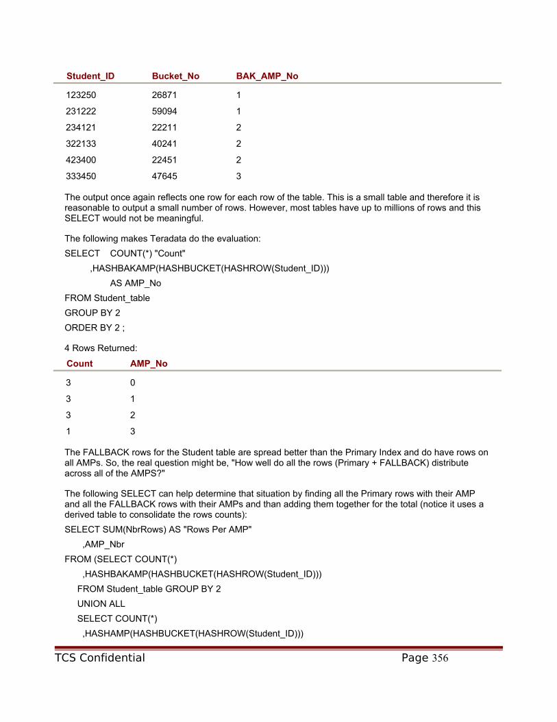
Student_ID Bucket_No BAK_AMP_No

123250 26871 1

231222 59094 1

234121 22211 2

322133 40241 2

423400 22451 2

333450 47645 3

The output once again reflects one row for each row of the table. This is a small table and therefore it is reasonable to output a small number of rows. However, most tables have up to millions of rows and this SELECT would not be meaningful.

The following makes Teradata do the evaluation:

SELECT COUNT(*) "Count"


AS AMP_No

FROM Student_table

GROUP BY 2

ORDER BY 2 ;

4 Rows Returned:

Count AMP_No

3 0

3 1

3 2

1 3

The FALLBACK rows for the Student table are spread better than the Primary Index and do have rows on all AMPs. So, the real question might be, "How well do all the rows (Primary + FALLBACK) distribute across all of the AMPS?"

The following SELECT can help determine that situation by finding all the Primary rows with their AMP and all the FALLBACK rows with their AMPs and than adding them together for the total (notice it uses a derived table to consolidate the rows counts):

SELECT SUM(NbrRows) AS "Rows Per AMP"

,AMP_Nbr

FROM (SELECT COUNT(*)


FROM Student_table GROUP BY 2

UNION ALL

SELECT COUNT(*)


TCS Confidential

FROM Student_table GROUP BY 2)

DT (NbrRows, AMP_Nbr)

GROUP BY 2

ORDER BY 2 ;

4 Rows Returned:

Rows Per AMP

AMP_Nbr

5 0

5 1

5 2

5 3

As seen here, the spread of both the primary data and the fallback data is very consistent. These are great functions to evaluate actual data distribution on the column(s) that are the primary index or any column can be used to test other distribution values.

Conclusion

Teradata makes it easy to create and drop tables. This chapter has discussed the fundamentals and advanced techniques to easily create and maintain the tables in a data warehouse. If you set up the table definitions correctly the first time then you will be well ahead of the game. Understand the simple examples used in the beginning part of this chapter first. That will get you started. Then, utilize the advanced techniques to maximize the flexibility Teradata provides to enhance your data warehouse environment.

Chapter 19: Temporary Tables

Temporary Tables

There may be times when an existing production database table does not provide precisely what you need. Sometimes, a particular query might need summarized or aggregated data. At other times, a small number of rows, from a very large table or data for a specific organization, are required to find an answer.

In a data warehouse with millions of rows, it might take too long to locate, derive or mathematically calculate the data needed. This is especially true when it is needed more than once per day. So, a view might not be the best solution or a view does not exist and you do not have the privilege to create one and both a view and derived table take too long. Any of these conditions prevent the ability to complete the request.

TCS Confidential

In the past, temporary tables have been created and used to help SQL run faster or be more efficient. They are extremely useful for solving problems that require stored "temporary"' results or which require multiple SQL steps. They are also great for holding aggregated or summarized data.

Most databases lose speed when they have to:Read every row in a very large table (full table scan)Perform several aggregationsPerform several data type conversionsJoin rows together from multiple tablesSort data

Temporary tables are often useful in a de-normalization effort. This might be done to make certain queries execute faster. Other times it is done to make the SQL easier to write, especially when using tools that generate SQL. However, these temporary tables are real tables and require manual operations to create, populate, and maintain them.

As a result, better name for these temporary tables might be interim or temporal tables. They exist for a specific period of time and when no longer needed, they are dropped to free up the disk space. During the interim time, they provide a valuable service. However, if the data in the original tables changes, the interim tables must be repopulated to reflect that change. This adds a level of difficulty or complexity regarding their use.

Creating Interim or Temporal Tables

The following series of commands provide an example of creating, inserting, and then entering SQL queries on an interim or temporal table (real table for short-term use):

CREATE TABLE Month_Sum_Sales

(Product_ID INTEGER

,Cal_Year SMALLINT

,Jan_sales DECIMAL(11,2)

,Feb_sales DECIMAL(11,2)

,Mar_sales DECIMAL(11,2)

,Apr_sales DECIMAL(11,2)

,May_sales DECIMAL(11,2)

,Jun_sales DECIMAL(11,2)

,Jul_sales DECIMAL(11,2)

,Aug_sales DECIMAL(11,2)

,Sep_sales DECIMAL(11,2)

,Oct_sales DECIMAL(11,2)

,Nov_sales DECIMAL(11,2)

,Dec_sales DECIMAL(11,2) )

UNIQUE PRIMARY INDEX (Product_ID, Cal_year);

This table breaks First Normal Form (1NF) in that it contains a repeating group for twelve monthly sales columns in every row. Normally, each row in a table represents an hour, a day, a week, or a month worth of sales. However with billions of rows, it requires extra time to read all the rows and consolidate them as calculated subtotals.

TCS Confidential

Therefore, the above table will make summary processing faster. In some cases, it will also make the SQL easier to write. Both of these become important considerations as the frequency of requests and the number of users needing this data, increases.

The Employee, Department and Sales tables below are used to demonstrate temporary tables:

Figure 19-1

Figure 19-2

TCS Confidential

Figure 19-3

To populate the interim table with data for September through December of the year 2000, the next INSERT / SELECT might be used:

/* Insert only September thru December into the table */

INSERT INTO Month_Sum_Sales

(Product_ID, Cal_year, Sep_Sales, Oct_sales, Nov_sales, Dec_sales)

SELECT Product_ID

,EXTRACT (YEAR FROM Sale_date)

,SUM(CASE ((Sale_date/100) MOD 100)

WHEN 9 THEN Daily_Sales ELSE 0 END)







FROM Sales_table

TCS Confidential

WHERE Sale_date BETWEEN 1000901 AND 1001230

GROUP BY 1,2;

Then, to display the sales for the last quarter of the year 2000, all that is required is a SELECT like the following:

SELECT Product_ID AS Product

,Cal_Year AS Cal_Yr

,Sep_sales AS September_sales

,Oct_sales AS October_sales

,Nov_sales AS November_sales

FROM Month_Sum_Sales

WHERE Cal_Year = 2000

ORDER BY 1 ;

3 Rows Returned

Product_ID Cal_Yr September_sales October_sales November_sales

1000 2000 139350.69 191854.03 0.00

2000 2000 139738.91 166872.90 0.00

3000 2000 139679.76 84908.06 0.00

The previous SQL shows how to create, insert, and access an interim table. Aside from the positive aspects of using this technique, there are other considerations. First, to provide current data, the rows in the table might need to be updated periodically. Otherwise, using active data warehouse tables and the summary table result in different answers to the same question.

Another issue regarding this technique is that a "real table" must be created and later it will be dropped manually. Both of these actions require updates in the Data Dictionary (DD). Additionally, you must have the privileges to CREATE and DROP a table as well as available Permanent space. Most data warehouse sites do not allow for this type of loose security and space management. It is not normally an acceptable practice to allow all users to create these temporal tables for this purpose.

Potential gains using an Interim table:

Make the SQL easier to write and run faster Avoid repeated aggregation on the real data rows Provide Primary Index access Data is available to multiple users

The associated costs of this table:

It requires separate steps to create and populate the table originally It must be kept updated with new sales data Requires extra PERM Space for the interim table Requires the table to be manually dropped when no longer needed Requires privileges to execute a CREATE and DROP TABLE Requires DD locking to create and drop table

TCS Confidential

The main problem is that a permanent table had to be created. This action is manual and is done within the DD because it is a real table. Another problem is that the contents of the table may quickly become out of date the moment a row changes in the original table.

The biggest single stumbling block is probably the inability to create a table, due to a lack of the proper privileges or Permanent space. The only solution is to submit a change request to the Database Administrator (DBA). Therefore, the process might take a couple of days to complete. This can be devastating when the data is needed immediately. So instead of using interim tables, this may be a perfect opportunity to use temporary tables.

Temporary Table Choices

There are three types of temporary tables available within Teradata. All of which have advantages over traditional temporary tables.

Derived tables are always local to a single SQL request. They are built dynamically using an additional SELECT within the query. The rows of the derived table are stored in spool and discarded as soon as the query finishes. The DD has no knowledge of derived tables. Therefore, no extra privileges are necessary. Its space comes from the users spool space.

Volatile Temporary tables are local to a session rather than a specific query. This means that the table may be used repeatedly within a user session. That is the major difference between volatile temporary tables (multiple use) and derived tables (single use). Like a derived, a volatile temporary table is materialized in spool space. However, it is not discarded until the session ends or when the user manually drops it. The DD has no knowledge of volatile temporary tables. They are often simply called, volatile tables; no extra privileges are required to use them either. Its space comes from the users spool space.

Global Temporary tables are local to a session, like volatile tables. However, they are known in the DD where a permanent definition is kept. Global temporary tables are materialized within a session in a new type of database area called temporary space. Also like volatile tables, they are discarded at the end of the session or when the user manually requests the table to be dropped. They are often called, global tables. Its space comes from a new type of space called temporary space.

Derived Tables

Derived tables were introduced into Teradata with V2R2. The creation of the derived table is local to the SQL statement and available only for a single request. However, a request may contain multiple derived tables. Once these tables are defined and populated, they may be joined or manipulated just like any other table. Derived tables become an alternative to creating views or the use of interim tables.

Derived tables are very useful. However, since they only exist for the duration of a single request, they may not be a practical solution if the rows are needed for multiple, follow-up queries needing the same data. The derived table is materialized in spool space, used and dropped automatically at the end of the query. Since it is entirely in spool, it only requires the user to have enough spool space. Since there is no DD involvement, special privileges are not required.

The process of deriving a table is much like deriving column data. They are both done dynamically in an SQL statement. The main difference is that column data is normally derived in the SELECT list, but derived tables are defined in the FROM. A derived table is created dynamically by referring to it in the FROM portion of a SELECT, UPDATE or DELETE. Like all tables, it needs a table name, one or more

TCS Confidential

column names and data rows. All of these requirements are established in the FROM portion of an SQL statement.

The following is the syntax for creating a derived table:

SELECT <column-name1> [ , <column-name2> [ ,<column-nameN> ] ]

FROM ( SELECT <column-name1> [ AS <alias-name> ]

[ ... ,<column-nameN> ] FROM <table-name> )

<Derived-table-name> [ ( <alias-name1> [...,<alias-nameN> ] )

;

In the above syntax, everything after the first FROM is used to dynamically name the derived table with its columns and populate it with a SELECT. The SELECT is in parentheses and looks like a subquery. However, subqueries are written in the WHERE clause and this is in the FROM. This SELECT is used to populate the table like an INSERT/SELECT for a real table, but without the INSERT.

The derived table and its columns must have valid names. If desired, the derived table column names can default to the actual column names in the SELECT from a real table. Otherwise, they can be alias names established using AS in the SELECT of the derived table, or specified in the parentheses after the name of the derived table, like in a CREATE VIEW. Using this technique is our preference. It makes the names easy to find because they are all physically close together and does not require a search through the entire SELECT list to find them.

These columns receive their data type from the columns listed in the SELECT from a real table. Their respective data types are established as a result of the sequence that the columns appear in the SELECT list. If a different data type is required, the CAST can be used to make the adjustment.

The following is a simple example using a derived table named DT with a column alias called avgsal and its data value is obtained using the AVG aggregation:

SELECT *

FROM (SELECT AVG(salary) FROM Employee_table) DT(avgsal) ;

1 Row Returned

avgsal

46782.15

Once the derived table has been materialized and populated, the actual SQL statement reads its rows from the derived table, just like any other table. Although this derived table and its SELECT are simplified, it can be any valid SELECT and therefore can use any of the SQL constructs such as: inner and outer joins, one or more set operators, subqueries and correlated subqueries, aggregates and OLAP functions. Like a view, it cannot contain an ORDER BY, a WITH, or a WITH BY. However, these operations can still be requested in the main query, just not in the SELECT for the derived table.

The best thing about a derived table is that the user is not required to have CREATE TABLE privileges and after its use. A derived table is automatically "dropped" to "clean up" after itself. However, since it is dropped the data rows are not available for a second SELECT operation. When these rows are needed in more than a single SELECT, a derived table may not be as efficient as a volatile or global temporary table.

The next example uses the same derived table named DT to join against the Employee table to find all the employees who make less than the average salary:

SELECT Last_name

TCS Confidential

,Salary

,Avgsal

FROM (SELECT AVG(salary) FROM Employee_table) DT(avgsal)

INNER JOIN Employee_table

ON avgsal < salary;

5 Row Returned

Last_name Salary Avgsal _

Chambers 48850.00 46782.15

Smythe 64300.00 46782.15

Smith 48000.00 46782.15

Harrison 54500.00 46782.15

Strickling 54500.00 46782.15

Now that avgsal is a column, it can be selected for display as well as being compared to determine which rows to return.

This derived table below is a bit more involved; it contains two columns and some number of rows created by doing an aggregation with a GROUP BY and then does aggregation on the aggregates in the derived table:

SELECT Derived_Col1

,SUM(Derived_Col2)

,AVG(Derived_Col2)

FROM (SELECT OthT_Col1, SUM(OthT_Col2) FROM Oth_Tbl

WHERE OthT_Col1 < 200 GROUP BY 1)

My_Derived_Tbl ( Derived_Col1, Derived_Col2 )

GROUP BY 1;

Both columns, Derived_Col1 and Derived_Col2, are named in parentheses following the derived table name, My_Derived_Tbl. The FROM is also used to populate My_Derived_Tbl via the SELECT using the table called Oth_Tbl. The derived table is then used to provide the aggregates of SUM and AVG on the column called Derived_Col2. The tables called Oth_Tbl and Payment_Table (later example) do not exist in my data tables. They are used here to illustrate the mechanics of more suffocated derived tables only and not executed to see the rows. Please continue reading the next paragraphs for a detail explanation regarding the usage of derived tables.

The data value for Derived_Col1 is obtained from data in the real column called OthT_Col1. It is selected as a non-aggregate and specified in the GROUP BY of the SELECT of the derived table; it follows normal aggregation rules. The derived table will contain one row for each unique value in OthT_Col1. Then, the column called Derived_Col2 is derived using the SUM aggregate on column OthT_Col2.

Therefore, the main SELECT in this query is from the derived table to perform a SUM and an AVG on the value obtained using a SUM of OthT_Col2. Like using a view, this is a fast, easy way to perform aggregation on aggregates.

This example uses a derived table to accomplish the same processing seen previously with an interim table:

TCS Confidential

SELECT Product_ID AS Product, Cal_yr

,Sep_sales AS September_sales

,Oct_sales AS October_sales

,Nov_sales AS November_sales

FROM (SELECT Product_ID ,EXTRACT(YEAR FROM Sale_date) AS Cal_Yr


WHEN 9 THEN Daily_Sales

ELSE 0

END) AS Sep_sales



ELSE 0

END) AS Oct_sales



ELSE 0

END) AS Nov_sales

FROM Sales_table

WHERE Sale_date BETWEEN 1000901 AND 1001130

GROUP BY 1,2)

DT_Month_Sum_Sales

/* The Derived table above is called DT_Month_Sum_Sales and gets its column names

from the alias names of the above SELECT in parentheses */

WHERE Cal_Yr = 2000

ORDER BY 1 ;

3 Rows Returned

Product_ID Cal_Yr September_sales October_sales November_sales

1000 2000 139350.69 191854.03 0

2000 2000 139738.90 166872.90 0

3000 2000 139679.76 84908.06 0

The next SELECT is rather involved; it builds My_Derived_Tbl as a derived table:

SELECT Derived_Col1

,Derived_Col2

,Payment_date

,Payment_amount

/* The Derived table definition starts below */

FROM (SELECT OthT1_Col1, OthT2_Col2, OthT1_Col3

FROM Oth_Tbl_1 AS OT1

TCS Confidential

INNER JOIN Oth_Tbl_2 AS OT2

ON OT1.Col3 = OT2.Col3

/* The correlated subquery to populate the Derived table starts below */

WHERE OT1.Sale_date = (SELECT MAX(Purchase_Date)

FROM Sales_Tbl

WHERE OT1.OthT1_Col3 = Sales_Product )

My_Derived_Tbl ( Derived_Col1, Derived_Col2, Derived_Col3 )

/* The Derived table definition ends here */

RIGHT OUTER JOIN Payment_Tbl AS PT

ON Derived_Col3 = Payment_Col5

/* The correlated subquery for the main SELECT starts below */

WHERE Payment_Date = (SELECT MAX(Payment_Date) FROM Payment_Tbl

WHERE Payment_Tbl.Account_Nbr=PT.Account_Nbr);

The derived table is created using an INNER JOIN and a Correlated Subquery. The main SELECT then uses the derived table as the outer table to process an OUTER JOIN. It is joined with the Payment table and uses a Correlated Subquery to make sure that only the latest payment is accessed for each account.

Whether your requirements are straightforward or complex, derived tables provide an ad hoc method to create a "table" with data rows and use them one time in an SQL statement without needing a real table to store them.

Volatile Temporary Tables

Volatile tables were introduced in release V2R3 of Teradata. They have two characteristics in common with derived tables. They are materialized in spool and are unknown in the DD. However, unlike a derived table, a volatile table may be used in more than one SQL statement throughout the life of a session. This feature allows other follow-up queries to utilize the same rows in the temporary table without requiring them to be established again. This ability to use the rows multiple times is their biggest advantage over derived tables.

A volatile table may be dropped manually at any time when it is no longer needed. If it is not dropped manually, it will be dropped automatically at the end of the user session. A user can materialize up to a maximum of 64 volatile tables at a time. Each volatile table requires its own CREATE statement. Unlike a real table with its definition stored in the DD, the volatile table name and column definitions are stored only in cache memory of the Parsing Engine. Since the rows of a volatile table are stored in spool and do not have DD entries, they do not survive a system restart. That is why they are called volatile.

The syntax to create a volatile table follows:

CREATE VOLATILE TABLE <table-name> [ , { LOG | NO LOG } ]

( <column-name1> <data-type>

[ , <column-name2> <data-type>

[ , <column-nameN> <data-type> ] )


[ ON COMMIT { PRESERVE | DELETE } ROWS ]

TCS Confidential

;The LOG option indicates the desire for standard transaction logging of "before images" in the transient journal. Without journaling, maintenance activities can be much faster. However, be aware that without journaling, there is no transaction recovery available. LOG is the default, but unlike real tables it can be turned off, by specifying: NO LOG.The second table option regards the retention of rows that are inserted into a volatile table.

The default value is ON COMMIT DELETE ROWS. It specifies that at the end of a transaction, the table rows should be deleted. Although this approach seems unusual, it is actually the default required by the ANSI standard. It is appropriate in situations where a table is materialized only to produce rows and the rows are not needed after the transaction completes. Remember, in ANSI mode, all SQL is considered part of a single transaction until it fails or the user does a COMMIT WORK command.

The ON COMMIT PRESERVE ROWS option provides the more normal situation where the table rows are kept after the end of the transaction. If the rows are going to be needed for other queries in other transactions, use this option or the table will be empty. Since each SQL request is a transaction in Teradata mode, this is the commonly used option to make rows stay in the volatile table for continued use.

Without DD entries, the following options are NOT available with volatile tables:

Permanent JournalingReferential IntegrityCHECK constraintsColumn compressionColumn default valuesColumn titlesNamed indexes

Volatile tables must have names that are unique within the user's session. They are qualified by the user-id of the session, either explicitly or implicitly. A volatile table cannot exist in a database; it can only materialize in a user's session and area.

The fact that a volatile table exists only to a user's session implies a hidden consequence. No other user may access rows in someone else's volatile table. Furthermore, since it is local to a session, the same user cannot access the rows of their own "volatile table" from another session, only in the original session. Instead, another session must run the same create volatile table command to obtain an instance of it and another SELECT to populate it with the same rows if they are needed in a second session.

Although this might sound bad, it provides greater flexibility. It allows for a situation where the same "table" is used to process different requests by storing completely different rows. On the other hand, it means that a volatile table may not be the best solution when multiple sessions or multiple users need access to the same rows on a frequent basis.

The following examples show how to create, populate, and run queries using a volatile table:

CREATE VOLATILE TABLE Dept_Aggreg_vt , NO LOG

( Dept_no Integer

,Sum_Salary Decimal(10,2)

,Avg_Salary Decimal(7,2)

,Max_Salary Decimal(7,2)

,Min_Salary Decimal(7,2)

,Cnt_Salary Integer )

TCS Confidential

ON COMMIT PRESERVE ROWS

;

The definition is built in the PE's cache memory. This is the only place that it resides, not in the DD.

The next INSERT/SELECT populates the volatile table created above with one data row per department that has at least one employee in it:

INSERT INTO Dept_Aggreg_vt

SELECT Dept_no

,SUM(Salary)

,AVG(Salary)

,MAX(Salary)

,MIN(Salary)

,COUNT(Salary)

FROM Employee_Table

GROUP BY Dept_no ;

Now that the volatile table exists in the cache memory of the PE and it contains data rows, it is ready for use in a variety of SQL statements:

SELECT * FROM Dept_Aggreg_vt

ORDER BY 1;

6 Rows Returned

Dept_no Sum_Salary Avg_Salary Max_Salary Min_Salary Cnt_Salary

? 32800.50 32800.50 32800.50 32800.50 1

10 64300.00 64300.00 64300.00 64300.00 1

100 48850.00 48850.00 48850.00 48850.00 1

200 89888.88 44944.44 48000.00 41888.88 2

300 40200.00 40200.00 40200.00 40200.00 1

400 145000.00 48333.33 54000.00 36000.00 3

The same rows are still available for another SELECT:

SELECT Department_Name

,Avg_Salary

,Max_Salary

,Min_Salary

FROM Dept_Aggreg_vt AS VT INNER JOIN Department_Table D

ON VT.dept_no = D.dept_no

WHERE Cnt_Salary > 1 ;

2 Rows Returned

TCS Confidential

Department_Name Avg_Salary Max_Salary Min_Salary


44944.44 48000.00 41888.88

Customer Support 48333.33 54000.00 36000.00

Whenever a single user needs data rows and they are needed more than once in a session, the volatile table is a better solution than the derived table. Then, as the user logs off, the table definition and spool space are automatically deleted.

Since no DD entry is available for a volatile table, they will not be seen with a HELP USER command. The only way to see how many and which volatile tables exist is to use the following command:

HELP VOLATILE TABLE ;

1 Row Returned

Session Id

Table Name

Table Id Protection Creator Name

Commit Option

Transaction Log

1010 my_vt 10C0C40000 N MIKEL P Y

The main disadvantage of a volatile table is that it must be created via the CREATE VOLATILE TABLE statement every time a new session is established. This situation can be overcome using a global temporary table.

Global Temporary Tables

Global Temporary Tables were also introduced in release V2R3 of Teradata. Their table and column definition is stored in the DD, unlike volatile tables. The first SQL DML statement to access a global temporary table, typically an INSERT/SELECT, materializes the table. They are often called global tables.

Like volatile tables, global tables are local to a session. The materialized instance of the table is not shareable with other sessions. Also like volatile tables, the global table instance may be dropped explicitly at any time or it is dropped automatically at the end of the session. However, the definition remains in the dictionary for future materialized instances of the same table. At the same time, the materialized instance or base definition may be dropped with an explicit DROP command, like any table.

The only privilege required to use a global table is the DML privilege necessary to materialize the table, usually an INSERT/SELECT. Once it is materialized, no other privileges are checked.

A special type of space called "Temporary space" is used for global temporary tables. Like Permanent space, Temporary space is preserved during a system restart and thus, global temporary tables are able to survive a system restart.

These global tables are created using the CREATE GLOBAL TEMPORARY TABLE command. Unlike the volatile table, this CREATE stores the base definition of the table in the DD and is only executed once per database. Like volatile tables, the table defaults are to LOG transactions and ON COMMIT DELETE ROWS. Up to 32 materialized instances of a global temporary table may exist for a single user.

Once the table is accessed by a DML command, such as the INSERT/SELECT, the table is considered materialized and a row is entered into a DD table called DBC.Temptables. An administrator may SELECT from this table to determine the users with global tables materialized and how many global tables exist.

Deleting all rows from a global table does not de-materialize the table. The instance of the table must be dropped or the session must be ended for the materialized table to be discarded.

TCS Confidential

The syntax to create a global temporary table follows:

CREATE GLOBAL TEMPORARY TABLE <table-name> [ { LOG | NO LOG } ]

( <column-name1> <data-type>

[ , <column-name2> <data-type> ]


[ ON COMMIT { PRESERVE | DELETE } ROWS ]

;

GLOBAL Temporary Table Examples

This series of commands show how to create, insert, and select from a global temporary table:

CREATE GLOBAL TEMPORARY TABLE Dept_Aggreg_gt

( Dept_no Integer

,Sum_Salary Decimal(10,2)

,Avg_Salary Decimal(7,2)

,Max_Salary Decimal(7,2)

,Min_Salary Decimal(7,2)

,Cnt_Salary Integer )

ON COMMIT PRESERVE ROWS

;

The next INSERT will create one data row per department that has at least one employee in it:

INSERT INTO Dept_Aggreg_gt

SELECT Dept_no ,SUM(Salary) , AVG(Salary) ,MAX(Salary) ,MIN(Salary)

,COUNT(Salary)

FROM Employee_Table GROUP BY Dept_no ;

Now that the global temporary table exists in the DD and it contains data rows, it is ready for use in a variety of SQL statements like the following:

SELECT * FROM Dept_Aggreg_gt

ORDER BY 1;

6 Rows Returned

Dept_no Sum_Salary Avg_Salary Max_Salary Min_Salary Cnt_Salary

? 32800.50 32800.50 32800.50 32800.50 1

10 64300.00 64300.00 64300.00 64300.00 1

100 48850.00 48850.00 48850.00 48850.00 1

200 89888.88 44944.44 48000.00 41888.88 2

300 40200.00 40200.00 40200.00 40200.00 1

400 145000.00 48333.33 54000.00 36000.00 3

It can immediately be used by other SELECT operations:

TCS Confidential

SELECT Department_Name

,Avg_Salary

,Max_Salary

,Min_Salary

FROM Dept_Aggreg_gt AS GT INNER JOIN Department_Table D

ON GT.dept_no = D.dept_no

WHERE Cnt_Salary > 1;

2 Rows Returned

Department_Name Avg_Salary Max_Salary Min_Salary


44944.44 48000.00 41888.88

Customer Support 48333.33 54000.00 36000.00

At this point, it is probably obvious that these examples are the same as those used for the volatile table except for the fact that the table name ends with "gt" instead of "vt." Volatile tables and global temporary tables are very much interchangeable from the user perspective. The biggest advantage to using the global temporary table lies in the fact that the table never needs to be created a second time. All the user needs to do is reference it with an INSERT/SELECT and it is automatically materialized with rows.

Therefore, when multiple users need the same definition, it is better to store it one time and give all users the INSERT privilege on it. It is the standard definition available to all users without requiring each user to run a CREATE statement and overcomes the main disadvantage of a volatile table. However, no user can access or disturb rows belonging to another user. They can only access their own rows due to each user session owning a different instance of the table.

Since the global temporary table's definition is stored in the DD, it may be altered using the ALTER command. It can change any attributes of the table, like real tables. Additionally, for extra flexibility, a materialized instance of the table may be altered without affecting the base definition or other user's materialized instance. Talk about flexibility.

This advantage means that a user is not restricted to having an identical definition as all other users. By using the ALTER TEMPORARY TABLE statement, the user can fine-tune the table for their specific needs, session by session.

Since a global temporary table can be altered and is not in spool space, this means that within an instance, it can take advantage of the following operations:

Add / Drop columns Add / Drop attributes Create / Drop indices Collect Statistics

As an example, if someone did not wish to use the LOG option for his or her instance, the next ALTER could be used:

TCS Confidential

ALTER TEMPORARY TABLE Dept_Aggreg_gt NO LOG;

Therefore, care should be taken to insure that not all users have ALTER privileges on the base table definition in the DD. Otherwise, accidentally omitting the word "temporary" alters the base definition and no one has the LOG option as seen below:

ALTER TABLE Dept_Aggreg_gt NO LOG;

Likewise, the same consideration should be used when defining and collecting Statistics on the stored definition versus the materialized instance. The following defines which statistics to collect on the table definition:

COLLECT STATISTICS ON Dept_Aggreg_gt index (Dept_no);

However, when this is executed there are no rows in the table and therefore no rows to evaluate and no statistics to store. So, why bother? The reason is that once an instance is materialized all a user needs to do is collect statistics at the table level after inserting their rows into their temporary instance of the table.

The following COLLECT specifies the importance of the word TEMPORARY to denote the instance and not the base definition:

COLLECT TEMPORARY STATISTICS on Dept_Aggreg_gt;

The above statement collects all statistics for rows in the volatile table, as defined by the base table. However, a user might wish to collect statistics on a column not originally defined for the table, such as Max_Salary. To accomplish this collection operation, the user could execute the next statement:

COLLECT TEMPORARY STATISTICS on Dept_Aggreg_gt COLUMN Max_Salary;

As a reminder, each instance can only be accessed by a single user and furthermore, only within a single session for that user. Like the volatile table, the same user cannot access rows from their own temporary table from a different session.

Also like a volatile table, a global table releases its temporary space and the instance when the user logs off. If the user wishes to manually drop the instance, use the following command:

DROP TEMPORARY TABLE Dept_Aggreg_gt ;

Again, the word TEMPORARY is very important because without it:

DROP TABLE Dept_Aggreg_gt ;

Will drop the base definition and cause problems for other users. Privileges should be established to prevent a user from accidentally dropping a global table definition.

With that being said, there might come a time when it is desired to drop the base definition. If the above DROP TABLE is executed, it will work unless a user has a materialized instance. One materialized instance is enough to cause the statement to fail. As an alternative, an ALL option can be added, as seen in the next statement, in an attempt to drop the definition:

DROP TABLE Dept_Aggreg_gt ALL ;

This works as long as a user is not in the middle of a transaction. Otherwise, the only option is to wait until the user's transaction completes and then execute the DROP again.

The above format for a Global table indicates the ability to define a primary index as either unique or non-unique. Additionally, since the definition is in the data dictionary, placing a UNIQUE constraint on one or more columns would also make the first unique column a UPI. This logic is the same for a real table.

TCS Confidential

General Practices for Temporary use Tables

The following are guidelines to consider when determining which type of "temporary" table to use. Most of the criteria are based on the number of users needing access to the data. The second issue is related to the frequency of use.

Multiple user access to a table:

Temporal or interim table(short-term real table)

Single user access to a table,

- Single ad hoc SQL use table:

Derived table

- Multiple SQL use table:

Volatile or Global temporary table

- Standardized, multiple SQL use table:

Global temporary table

Use these guidelines to decide which type of table to use based on the needs of the user.

TCS Confidential

Chapter 20: Trigger Processing

Triggers

A trigger is an event driven maintenance operation. The event is caused by a modification to one or more columns of a row in a table. The original modification request, the trigger and all subsequent triggers constitute a single transaction. This means that the SQL and all triggered statements must work successfully, or else, all fail and rollback all changed rows from the Transient Journal.

Triggers are an excellent way to automate many database modifications that previously required manual intervention by the user or DBA. Since triggers occur automatically, they remove the burden from a person's memory to make the subsequent updates in one or more other tables. Therefore, they can be used as a labor savings device and improve data integrity at the same time, two benefits in one.

Triggers can be particularly useful when Referential Integrity (RI) is defined. Teradata incorporates the Prevent logic as its strategy for handling any SQL request that attempts to modify a column with new data that violates RI. Triggers can be established to implement either the Cascade or Nullify strategies.

Triggers are a new form of object in the Teradata database. They are designated with a type of "G" seen with a HELP DATABASE request. My guess is that the developers could not use "T" because of tables and the "RI" reminded them of referential integrity, so "G" was the next character in TRIGGER. The DDL statements used with triggers are: CREATE, DROP, REPLACE, ALTER, HELP and SHOW. These statements manage trigger usage and maintenance. The appropriate database privileges are needed to use any of these commands.

Terminology

Triggering Statement

The user's initial SQL maintenance request that causes a row to change in a table and then causes a trigger to fire (execute).

It can be: INSERT, UPDATE, DELETE, INSERT/SELECT

It cannot be: SELECT

TCS Confidential

Triggered Statement

It is the SQL that is automatically executed as a result of a triggering statement.

It can be: INSERT, UPDATE, DELETE, INSERT/SELECT, ABORT/ROLLBACK, EXEC

It cannot be: BEGIN/END TRANSACTION, COMMIT, CHECKPOINT, SELECT

Logic Flow

The operations performed by a trigger are defined in the Data Dictionary (DD) and stored as an SQL object. Whenever a user issues any SQL request that modifies a row, a column or table that has a trigger defined on it, the trigger SQL is eligible to also execute.

It becomes the "memory" for all subsequent update operations without a person needing to remember to make the appropriate changes on one or more other tables.

The original user SQL is the triggering statement on the Subject table. The subsequent, automatic update to a different table is the triggered statement.

TCS Confidential

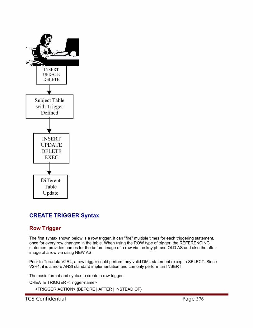
CREATE TRIGGER Syntax

Row Trigger

The first syntax shown below is a row trigger. It can "fire" multiple times for each triggering statement, once for every row changed in the table. When using the ROW type of trigger, the REFERENCING statement provides names for the before image of a row via the key phrase OLD AS and also the after image of a row via using NEW AS.

Prior to Teradata V2R4, a row trigger could perform any valid DML statement except a SELECT. Since V2R4, it is a more ANSI standard implementation and can only perform an INSERT.

The basic format and syntax to create a row trigger:

CREATE TRIGGER <Trigger-name>

<TRIGGER ACTION> {BEFORE | AFTER | INSTEAD OF}

TCS Confidential

[ ORDER <sequence-number> ]

<TRIGGERING ACTION > {INSERT | UPDATE | DELETE | INSERT/SELECT}

[ OF (<column-name>, ... ) ] ON <subject-table>

REFERENCING OLD AS <before-imaged-row>

NEW AS <after-image-row>

FOR EACH ROW

[ WHEN (optional condition) ]

( <TRIGGERED ACTION> { INSERT | INSERT/SELECT} ; )

;

Additional discussion and examples are presented to enhance understanding of trigger use after a discussion of a Statement trigger.

Statement Trigger

The second syntax below is for a STATEMENT trigger. It will only fire once for each triggering statement. When using the STATEMENT type of trigger, the REFERENCING will use OLD_TABLE for all before image rows and NEW_TABLE for all after image rows.

The basic format and syntax to create a statement trigger:

CREATE TRIGGER <Trigger-name>

<TRIGGER ACTION> {BEFORE | AFTER | INSTEAD OF}

[ ORDER <sequence-number> ]

<TRIGGERING ACTION > {INSERT | UPDATE | DELETE | INSERT/SELECT}

[ OF (<column-name>, ... ) ] ON <subject-table>

REFERENCING OLD_TABLE AS <before-image>

NEW_TABLE AS <after-image>

FOR EACH STATEMENT

[ WHEN (optional condition) ]

( <TRIGGERED ACTION> { INSERT | INSERT/SELECT | UPDATE | DELETE |

ABORT/ROLLBACK | EXEC } ; ) ;

To CREATE a trigger, a unique name must be chosen within a database for the new object. Then, chose a trigger action from the three types to dictate when the trigger will execute, they are: BEFORE, AFTER, and INSTEAD OF. The implication here regards when the trigger fires. It either fires BEFORE the user request, AFTER the user request or INSTEAD OF the user request.

The optional ORDER designation is used to sequence the firing of triggers. This is only a consideration when more than one trigger is based on the same trigger action (BEFORE, AFTER or INSTEAD OF). For instance, if there is one BEFORE and one AFTER trigger, then logically the BEFORE fires first and the AFTER fires last. For more information on ORDER, see the Sequencing Triggers section later in the chapter.

Next, determine the action that is to cause the trigger to execute. There are four types of SQL triggering statements that can cause a trigger to fire, they are: INSERT, INSERT/SELECT, UPDATE, and DELETE.

TCS Confidential

When the triggering statement is an UPDATE, the optional OF portion is probably needed. It names one or more specific column(s) to monitor for a change in the data. If data, in all columns named in the OF, is changed the trigger will fire. Otherwise, if the data is changed in only one of the columns, the trigger does not fire. It is all or nothing regarding the columns being monitored for a change. When the OF is not used, the value in every column must change in order for the trigger to fire.

The table name specified by the ON is referred to as the subject table. It is the table to be changed by the triggering statement (user request). A trigger can only have one subject table.

Although there are both OLD AS and NEW AS references, they are only be used together when an UPDATE is the triggering statement. The UPDATE must have an existing row to modify. Therefore, a before image and a modified after image both exist.

When the triggering statement is an INSERT, there is only a NEW AS reference name because there is only a new row and not an old row. Conversely, when the triggering statement is a DELETE, there is only an OLD AS reference name because the row no longer exists.

The optional WHEN designator provides a last conditional test to make before actually executing the trigger. For instance, it might check the time of day or perform a subquery (only place a SELECT is allowed) to check for a specific value, such as an IN or NOT IN. As an example, a test might be performed to determine the amount of work involved using a COUNT and if too many rows are involved, delay the triggering statement until later. The trigger will fire only if the WHEN test compares true.

Lastly, determine the TRIGGERED ACTION. It is an SQL triggered statement that will execute as a result of the triggering statement. There are six SQL statements that can be a triggered statement, they are: INSERT, INSERT/SELECT, UPDATE, DELETE, EXEC and ABORT/ROLLBACK. Remember that a trigger is part of a transaction and cannot begin a new transaction.

‘BEFORE’ Trigger

The BEFORE trigger is executed prior to the maintenance requested by the user's client application. Once the trigger has successfully completed, the actual modification of the row(s) in the subject table is done for the user.

The following creates a BEFORE trigger on the Employee table to provide a Cascade form of RI by making sure that the Department table contains the department in which the new employee works:

CREATE TRIGGER RI_Cascade_Trig

BEFORE INSERT ON Employee_table

REFERENCING NEW AS aftrow

FOR EACH ROW

WHEN ( aftrow.dept_no NOT IN (SELECT Dept_no FROM Valid_Dept_table))

(INSERT INTO Department_table

VALUES (aftrow.dept_no, 'New Department',NULL,NULL);) ;

This is a row trigger because it contains FOR EACH ROW. It is executed once for each row inserted into the Employee table and each triggered INSERT only inserts a single row if the department for the new employee is not a valid department verified against the department table. This request is not allowed if the subquery in the WHEN references the subject table. Therefore, the Valid_Dept_table is required to allow that test.

Other than checking another table, a BEFORE trigger might be useful for making an adjustment in another table before making the final modification in the subject table. In other words, if the update might cause a

TCS Confidential

RI error, the trigger can prepare the other table to conform to an RI constraint before the original update gets rejected. For instance, if a Department were being deleted, the trigger could change the department number for all employees to NULL before the deletion of the department row. This is an example of the Nullify Strategy for RI.

‘AFTER’ Trigger

The AFTER trigger is executed or fired subsequent to the original update requested by the user's client application. Once the trigger has successfully completed, the user request part of the transaction is finished.

The following creates an AFTER trigger on the Parts table to insert an audit row into the Price Log table if the price is changed. However, the trigger only fires if the increase is greater than 10%:

CREATE TRIGGER Update_Trig

AFTER UPDATE OF (price) ON parts

REFERENCING OLD AS beforerow

NEW AS afterrow

FOR EACH ROW

WHEN ( (afterrow.price - beforerow.price) / beforerow.price > .10)

( INSERT INTO price_log values (afterrow.part_num, beforerow.price,

afterrow.price, date); ) ;

This is also a row type of trigger. Therefore, it will be executed once for each and every row that is affected by the original update SQL request.

Here a WHEN determines whether or not the trigger fires. For small price increases, the trigger does not fire, but instead, only for a price change of more than 10%. Without a WHEN test, the trigger fires every time the triggering statement makes a change.

An AFTER trigger is helpful to make an adjustment in one table based on a change made to the subject table. For instance, if a new manager were assigned to a department in the department table, all the rows for employees are updated automatically to reflect the same change in the employee table. This is an example of the Cascade Strategy for RI.

‘INSTEAD OF’ Trigger

The INSTEAD OF trigger provides the ability to execute the trigger and not do the user's client application request at all. Once the trigger has successfully completed, the transaction is finished.

The following INSTEAD OF trigger is created on the parts table to insert an audit row into the delay table indicating that an UPDATE on the parts table should have taken place. However, because it was going to impact more than 10 rows in the subject table, it was not performed:

CREATE TRIGGER DelayUpd

INSTEAD OF UPDATE OF (price) ON parts

REFERENCING OLD_TABLE AS oldtab

NEW_TABLE AS newtab

FOR EACH STATEMENT

WHEN ( 10 < (SELECT COUNT(part_num) FROM oldtab

TCS Confidential

WHERE part_num = oldtab.part_num) )

( INSERT INTO Delay_Tab

SELECT DATE, TIME, 'Upd', newtab.part_num, newtab.price

FROM newtab WHERE newtab.part_num = part_num ; ) ;

Since the update on the parts table was not performed, it probably needs to be made at another time. This actual update becomes someone's responsibility. This is a time when the flexibility to not make the change adds responsibility to manually make the change later. However, the rows in the delay table can be used via a join to actually make the update.

Cascading Triggers

A cascading trigger results when a triggering statement fires a trigger, which in turn fires another trigger. The situation is such that the table being updated by the first trigger also has a trigger associated with it and becomes the new subject table. Then the second trigger updates a table that has a trigger associated with it. So, each triggered statement in turn becomes a triggering statement.

The only thing a trigger cannot do is to change the subject table on which the trigger is defined. However, a subsequent trigger may come back and update the original subject table. Caution should be exercised here so that the triggers do not cascade indefinitely. This constitutes an infinite loop and will cascade until they run out of either Permanent or Transient Journal space, or the transaction is aborted.

TCS Confidential

Cascading Trigger example:

In this cascade example, there are three tables: CasTbl_1, CasTbl_2 and CasTbl_3. Each table is defined with two columns called: Col1 and Col2. At the beginning of the process, all three tables are empty.

All three tables use basically the same CREATE TABLE to build the initial definitions; only the names have been changed.

CREATE TABLE CasTbl_1

(Col1 smallint, Col2 smallint);





TCS Confidential

Now the triggers are defined to monitor the rows in the tables called CasTlb_1 and CasTbl_2:

CREATE TRIGGER CasTrig1

AFTER INSERT ON CasTbl_1

REFERENCING NEW AS afterrow

FOR EACH ROW

( INSERT INTO CasTbl_2 values (afterrow.col1+1, afterrow.col2*2); ) ;

CREATE TRIGGER CasTrig2

AFTER INSERT ON CasTbl_2


FOR EACH ROW

( INSERT INTO CasTbl_3 values (afterrow.col1+1, afterrow.col2*2); ) ;

Now that the tables and triggers have been defined, the trigger statement can be issued:

INSERT INTO CasTbl_1 values (1, 4);

The next SELECT operations are to verify that the triggers worked:

SEL * FROM CasTbl_1;

1 Row Returned

Col1 Col2

1 4

The above output is from the original insert into the first table.

Look what happens when a SELECT is performed on each of the other two tables:

SEL * FROM CasTbl_2;

1 Row Returned

Col1 Col2

2 8

SEL * FROM CasTbl_3:

1 Row Returned

Col1 Col2

3 16

The first trigger inserted a row into CasTbl_2 as a result of the original insert into CasTbl_1. Then, the second trigger inserted a row into CasTbl_3 because of the inserted row into CasTbl_2. All of this happened as a result of the original INSERT; they cascaded from the original row.

Remember the one thing to avoid when using cascading triggers. Do not create a trigger on either CasTbl_2 or CasTbl_3 that will insert a row into CasTbl_1. This causes an indefinite loop of the INSERT operations that will continue until aborted.

TCS Confidential

Sequencing Triggers

All of the previously discussed triggers were independent from each other because the are on different tables and have a different ACTION. Therefore, the sequence in which they are fired does not matter. However, sometimes the sequence does matter. When this is the case, another mechanism must be used to guarantee that the triggers are fired in the proper sequence to insure that all modifications are made in the correct ORDER.

The ORDER option allows for the definition of a sequence number to be associated with each trigger. Valid values are 1 through 32,767. All triggers with an ORDER of 1, fire before the first ORDER 2 trigger. All the ORDER 2 triggers fire before the first 3 and so on until there are no more triggers associated with the initial triggering statement.

This ORDER process continues until there are no more triggers, or until a triggered action fails. Remember, that triggers are always part of a transaction and if part of a transaction fails, it stops and every operation to that point must ROLLBACK. When ORDER is not specified, it defaults to a value of 32,767. Triggers with the same ORDER value fire randomly until the last one with that same value finishes.

As an example, instead of using the cascading triggers seen previously, it might be desirable to have both triggers defined on CasTbl_1. That way, no INSERT need be performed on CasTbl_2, only on CasTbl_1, as seen with the two triggers created below:

CREATE TRIGGER INSTrig1

AFTER INSERT ON CasTbl_1 ORDER 100


FOR EACH ROW

( INSERT INTO CasTbl_2 values (afterrow.col1+1, beforerow.col2*2) ;

CREATE TRIGGER INSTrig2

AFTER INSERT ON CasTbl_1 ORDER 200


FOR EACH ROW

( INSERT INTO CasTbl_3 values (afterrow.col1+2, beforerow.col2*4) ;

Since both of the above triggers are AFTER INSERT, they both have the same trigger action. In this example, it was decided that INSTrig1 should fire before INSTrig2 because its value in the ORDER is less. The result will be identical if the ORDER is not specified for INSTrig2 because the value of 100 is less than 32,767. Using the ORDER allows this level of control, but it is optional and only needed to control sequencing. Without the ORDER, they are both 32,767 and fire randomly.

Chapter 21: Stored Procedures

Teradata Stored Procedures

Compatibility: ANSI

TCS Confidential

In Version 2 Release 4, Teradata provides Stored Procedural Language (SPL) to create Stored Procedures. These procedures allow the combination of both SQL and SPL control statements to manage the delivery and execution of the SQL.

Teradata used always had a scripting language in its utilities, such as BTEQ, to manage loops, conditional tests and processing on the host computer. To differentiate SQL and the scripting language, most of the utilities use a dot (.) command and the Teradata Call Level Interface (CLI).

Later, more standard tools were introduced to access rows stored within Teradata. Instead of using the Call Level Interface directly, they call the Open Data Base Computing (ODBC) software for connectivity across a network.

The call structure for the ODBC is standard. Most database vendors provide an ODBC executable for their database to convert the ODBC calls into calls for the proprietary CLI. The advantage of this technique becomes apparent in that more tools are made available to all users to access any database that has an ODBC connection. However, because these tools are interactive and ODBC based, they do not normally have a scripting language.

One of the advantages to stored procedures is that they are stored and executed within the Teradata database and not as a separate utility on a different computer. Therefore, the SPL commands are available for execution from all tools and not just those with their own scripting language.

Stored procedures constitute a major departure from the way "normal" SQL works within Teradata, like a macro. The following chart lists the differences between macros and stored procedures.

Figure 21-1

Writing a stored procedure is more like writing a program than writing a macro. The macro contains only SQL and maybe dot commands that are only for use in BTEQ. Normally a SELECT results in rows being returned to the user. A stored procedure does not return rows to the user like a macro. Instead, the selected column or columns must be used within the procedure.

A stored procedure contains SQL to access data from within Teradata. However, it must contain SPL to control the execution of the SQL. A stored procedure is a bit like writing a script in the Support Environment front-end for MultiLoad, TPump or FastExport. The major difference with stored procedures is that the language is much more comprehensive, allows the SELECT and is ANSI standard.

Like a macro, stored procedures allow parameter values to be passed to it at execution time. Unlike a macro that allows only input values, a stored procedure also provides output capabilities. A stored procedure only returns output values to a user client as output parameters, not as rows.

We normally think of the client as being the requestor and Teradata being the server. When using stored procedures, another layer is added. When a procedure is called, it is a server to the user program. However, it normally interfaces with Teradata on the behalf of the client. The only way to do that is to become a client too. So, a procedure plays both roles. This is a 3-tiered environment where: Tier 1 is the user as a client, Tier 2 is the procedure as first a server and then as a client and Tier 3 is Teradata as a server. The procedure acts as a server/client in that it is first a server to the user and then a client to Teradata in order to retrieve one or more rows to service the user request.

TCS Confidential

The processing flow of a procedure is more like a program. It is a procedural set of commands, where SQL is a non-procedural language. As mentioned earlier, it does not return rows to the user. Therefore, the use of a SELECT, UPDATE or DELETE statement that processes multiple rows will need to be managed within the stored procedure. In other words, you cannot code a simple procedure with SELECT * FROM <table-name>. A procedure is not a macro and a macro is not a stored procedure.

The intent of this chapter is to show and explain the commands as well as the technique for a successful implementation of procedures. It provides a basis to understand and begin to use stored procedures. The syntax for SPL is very flexible and powerful. So, each command will be discussed individually with an example demonstrating it. The examples will increase in complexity and functionality as more SPL commands are introduced.

Although DDL is not allowed within a procedure, DDL must be used to implement a stored procedure. The DDL is used to CREATE a procedure. Additionally, you will need a recent release of Queryman and the ODBC in order for the CREATE PROCEDURE statement to be recognized and sent to Teradata.

CREATE PROCEDURE

A stored procedure is created like all Teradata objects. However, it is stored as an executable piece of code. To be executable, it must be compiled as part of the CREATE request. Once compiled, the SPL is stored in a user database as an object. It is a new kind of object and seen as a "P" when using a HELP USER or HELP DATABASE request.

The following is the basic syntax to CREATE a procedure:

CREATE PROCEDURE [<database-name>.]<procedure-name>

( [ <parameter-list> ] )

<procedure-body>

;

The <parameter-list> is optional. When used, it allows parameter values to be sent to the procedure. They also allow for parameter values to be passed back to the client. Most of the time, a procedure will use parameters.

The <procedure-body> contains the SPL coding necessary to accomplish the processing desired of the stored procedure.

Stored Procedural Language (SPL) Statements

Within the create request of a procedure, called the procedure body, there will normally be Data Manipulation Language (DML) and SPL. Using Data Definition Language (DDL) and Data Control Language (DCL) is not currently permitted within a procedure.

The DML has already been covered in this book. This chapter primarily concentrates on the SPL. The only exception will be a discussion on SELECT, UPDATE and DELETE regarding cursors and the new SELECT-INTO for setting initial values of variables in a procedure.

The <procedure-body> may contain any or all of the following SPL commands:

BEGIN / END — Defines scope and functionality of the procedure body

TCS Confidential

CALL – Executes a procedure from a procedureDECLARE – Optional, establishes local variables or handler routines for use within the

procedureFOR / END FOR – Allows for a cursor to process commands for each row fetched from

Teradata IF / END IF - Provides for a conditional test of a variable ITERATE - Skips rest of the statements after the iterate statement and continues with the

iteration of the logicLEAVE – Allows for an exit from a loopLOOP / END LOOP – Defines the processing logic to repeat unconditionallyPRINT – Aids in testing and debugging of a new procedureSET – Assigns a value to a variable or parameterWHILE / END WHILE – Establishes a conditional test prior to doing a logic loop

These commands have been listed above in alphabetic sequence. They are normally written in a sequence to accomplish a specific task. Each of these is discussed below in more detail with examples to demonstrate their functionality.

The syntax of the <procedure-body> must contain a BEGIN and END combination statement formatted as:

[ <label-name>:] BEGIN

[ <local-variable-declaration> ]

[ <condition-handler-declaration> ]

[ <statement-list> ]

END [ <label-name> ]

;

BEGIN / END Statements

The BEGIN and END specifications are both required and they define the body of the procedure. All other SPL commands will be contained within the boundaries delineated by these two statements. Again, they are both required and because of the dependency on each other, they are referred to as a compound statement

The following is the syntax of the BEGIN and END commands:

[ <label-name>: ]BEGIN

END [ <label-name> ] ;

Optionally, a BEGIN may specify a label name to identify the SPL section within the procedure. When a label name is desired, it connects to the BEGIN via a colon (:). The END will only use a label name if one is defined on the BEGIN. A label name is optional whenever there is a single section of SPL. When multiple sections (more than one BEGIN and END statements) are used, the interior sections must have a label name.

The next table is used in the next examples:

TCS Confidential

Figure 21-2

Figure 21-3

The following demonstrates a simple procedure with a single section used to INSERT a row with all null values into the Customer table:

CREATE PROCEDURE First_Procedure ( )

BEGIN

INSERT INTO Customer_table WITH DEFAULT VALUES;

END;

After the execution of the above procedure, the next SELECT returns:

SELECT * FROM CUSTOMER_TABLE;

6 Rows Returned


? ? ?


555-1234

31313131 Acme Products 555-1111


57896883 XYZ Plumbing 347-8954

87323456 Databases N-U 322-1012

Notice that a separate SELECT (outside the procedure) is needed to see the row of null values instead of returning them from the procedure. The only output to the client from the execution of this procedure is a resultant status code. It indicates either a successful completion or a failure in the procedure.

More discussion will appear in this chapter to explain why this is the case. For now, suffice it to say that a stored procedure can't return rows to the client as noted in Figure 21-1.

The following demonstrates a technique to nesting one section within another using a label name on the inner section:

CREATE PROCEDURE First_Procedure ( )

TCS Confidential


BEGIN

INSERT INTO Customer_table WITH DEFAULT VALUES;

SecondSection:BEGIN

DELETE FROM Order_table WHERE Customer_number is NULL;

END SecondSection;

END;

In both of these examples, the indentation is optional and used by us to assist in understanding how the coding works. The first section does not use the optional label for the BEGIN and END. It contains an INSERT into the Customer table. Then, another BEGIN and an END called SecondSection is used. This SPL section contains a DELETE from the order table. The END for SecondSection comes before the END for the first BEGIN and specifies the label name SecondSection as defined in the BEGIN. It is nested within the first BEGIN and last END as compound statements.

The normal flow is from top to bottom. So, the customer INSERT is performed first, then the order DELETE is performed. Although this same processing occurs without a nested BEGIN / END for SecondSection, it introduces this technique for use with other commands covered below and the ability to allow repeated processing of one or more sections. It may not always be desirable to repeat all the commands, only specific ones. The procedure must be written to manage all desired processing.

Like all CREATE statements, the procedure name may be qualified to request its creation in a particular database. The parameter list is optional as in a macro. However, the parentheses are not optional and must be coded, even without parameters. When used, the parameters are normally included to make the procedure more flexible and provide communications with the outside world regarding each execution. The procedure body contains SPL to manage the execution of the SQL. The setup and use of parameters and SPL is covered progressively in this chapter to facilitate learning how to use SPL.

Establishing Variables and Data Values

A stored procedure can be written to provide additional functionality by naming local variables to store and manipulate values. The variables receive their values either by being explicitly assigned internally or passed from the client that calls the procedure. A SET statement is used to assign a value to a variable within a procedure. The value may be a literal or an equation. However, before using a variable name, the name and the data type must be defined. A DECLARE statement is used to establish the variable. Both of these commands are covered next.

DECLARE Statement to Define Variables

The DECLARE is primarily used to establish a local variable name for use within the stored procedure. The variable is called a local because the name is only available within the procedure.

The syntax for defining one or more variables is:

DECLARE <variable-name-list> <data-type> [ DEFAULT <initial-value> ] ;

The variable name list may contain one or more variable names. However, only a single data type may be defined within an individual DECLARE statement. So, if three variables are needed and each one is a different data type, three DECLARE statements are required. However, if all three variables are of the same data type, only a single DECLARE is needed. At the same time, it is permissible to use one DECLARE for each variable regardless of its data type. This might be the case when all three variables need to start with an different initial value in each one using the DEFAULT.

TCS Confidential

Two variables in the same procedure may not have the same name. Names must be unique within procedures just as they must be unique within a macro or database. Additionally, a variable name cannot be any of these reserved Status variable names:

SQLCODE SQLSTATE ACTIVITY_COUNT

The data type declared must be valid within Teradata, like in a CREATE TABLE request.

Optionally, a DEFAULT value may be specified. When this is done, every time the procedure is executed, the variable is automatically be set to the value specified. Otherwise, it will contain a NULL value. The DEFAULT value, if specified, applies to all variables specified in a single DECLARE statement.

The scope or validity of a local variable is the BEGIN/END block. Access to the value in a local variable is not directly available from outside of the procedure. A local variable may be used within SQL. When it is specified in an SQL statement, it must be prefixed with a colon (:). The colon indicates that substitution is to occur. At execution time, the value stored in the variable is substituted into the SQL in place of the name. Then, the SQL statement is executed.

The next procedure defines var1 as a local variable and assigns an initial value using a DEFAULT and then substitutes the value into the WHERE clause of a DELETE:

CREATE PROCEDURE Second_Procedure ( )

BEGIN

DECLARE var1 INTEGER DEFAULT 11111111;

DELETE FROM Customer_table WHERE Customer_number = :var1;

END;

This example is only a building block approach to writing stored procedures. This procedure is not flexible enough to delete any other row from the table. Therefore, it is a single use procedure. A procedure is most beneficial when it is used multiple times by multiple users. By incorporating other SPL and SQL, it will evolve into a useful procedure.

SET to Assign a Data Value as a Variable

The SET statement is an assignment statement. Once the variable name and data type have been defined, a value needs to be assigned. As seen above, the DEFAULT can establish an initial value. Otherwise, a value can be assigned or SET within the procedure. Then, it may retain the initial value throughout the life of the procedure, or may be modified at any time using a SET command.

The syntax for the SET statement follows:

SET <assignment-target> = <assignment-source> ;

The assignment target can be either a local variable or a parameter. Parameters are covered later.

The assignment source can be any of the following: a literal value, a local variable, a status variable, a parameter, an SQL CASE expression, a cursor, a column, an alias name, or a mathematical expression.

The following is an alternate Second_Procedure used to SET the value instead of using DEFAULT:

TCS Confidential

CREATE PROCEDURE Second_Procedure ( )

BEGIN

DECLARE var1 INTEGER ;

SET var1 = 11111111 ;


END;Even the SET by itself is still limited, the next section provides the best technique for assigning data values to a procedure with values passed as parameters.

Status Variables

These status variables are provided within the procedure body to determine the outcome of operations requested: SQLSTATE

SQLCODE

ACTIVITY_COUNT

CHAR (5)

SMALLINT

DECIMAL (18, 0)

A successful completion will assign the value of zero to each of the SQLSTATE and SQLCODE variables. Since SQLSTATE is a CHAR field, it will be ‘00000’ for comparison purposes. Other values should be referenced in the V2R4 Reference manual to determine what occurred for debug or correction purposes.

There is another reserved name for use in determining that an SQL error occurred. Its name is SQLEXCEPTION and is handy in checking for any non-zero outcome. It becomes the unknown or unspecified outcome, but is still considered an error condition. Checking for one or more specific outcomes is the purpose of SQLSTATE.

Again, these are all "read only" variables and cannot be used in the SET assignment statement as the assignment target.

Assigning a Data Value as a Parameter

Like macros, stored procedures may receive information passed from the client software. This ability provides much more flexibility and enhances the power of stored procedures.

Unlike macros, a stored procedure can return a parameter value to the calling user or routine. A macro can only return the output rows from a SELECT or status code to indicate the success or failure of the macro. This parameter output capability allows the stored procedure a way to offer functionality different than a macro. Depending on the functionality needed, either a macro or a stored procedure might be written.

When using parameters in a stored procedure, the syntax for a parameter list is comprised of these three elements:

<parameter-usage> <parameter-name> <data-type>

Where each element is defined as: <parameter-usage> can be one of these:

o IN only provides input from the caller (default)o OUT only provides output to the callero INOUT allows both input and output for the caller

TCS Confidential


<parameter-name> is any valid Teradata SQL name <data-type> is any valid Teradata data type

The following is an alternative to and a better version of Second_Procedure that passes the value for var1 instead of using a DECLARE or SET:

CREATE PROCEDURE Second_Procedure (IN var1 INTEGER )

BEGIN


END;

The value of var1 dynamically comes from the client at execution time. It is no longer fixed by the DECLARE or the SET commands. The flexibility now exists within Second_Procedure to delete any row from the table. Furthermore, there is no requirement to change the procedure every time a different row need s to be deleted. The CALL statement for this procedure appears in the next section along with a discussion on its use and the passing of parameter values.

Considerations for parameter definition:

A parameter is valid throughout the entire stored procedure If a parameter is referenced within an SQL statement, it must be prefixed with a colon (:) to

tell the optimizer that it is a variable name and not an object name A parameter name cannot be any of these names since they are reserved for status

variable names:o SQLCODEo SQLSTATEo ACTIVITY_COUNT

The DEFAULT clause cannot be specified for parameters to establish an initial value IN parameters cannot be part of the assignment target for any SPL or SQL statement OUT parameters cannot be part of the assignment source for any SPL or SQL statement

Additional SPL Statements

This section of the book discusses and demonstrates the SPL commands allowed within the body of the stored procedure. The first thing to notice is that they are not covered below in alphabetic sequence; like the list above.

We struggled with this departure. However, it is done in this manner to gradually build up to the more involved capabilities of the commands, like using a FOR loop. We believe you will be grateful for this approach by the end of the chapter.

CALL Statement

The CALL is used to execute a stored procedure. The CALL statement is normally executed either by a client program or interactively by a user. Additionally, a stored procedure is allowed to call another stored procedure.

The syntax to CALL a stored procedure:

CALL [<database-name>.]<stored-procedure-name> ( [<parameter-list> ] ) ;

TCS Confidential


The procedure name can be qualified with a database name to guarantee the correct procedure is used. A parameter list is only used when the procedure is expecting IN parameter values passed to it. The list must match the exact number of parameters in the procedure. Remember, even if you are not passing parameter values in the parameter list, you must still code the ( ) open parenthesis and close parenthesis to call the procedure.

The following CALL executes the first procedure shown above:

CALL First_Procedure ( );

Since the First_Procedure does not define any parameters, none are passed to it. However, Second_Procedure has evolved to the point of expecting a parameter the value at run time to identify the row to delete. The next CALL executes the Second_Procedure and passes the value of 11111111:

CALL Second_Procedure(11111111);

Now, the procedure can be called again and a different row can be deleted using:

CALL Second_Procedure(31313131);

This is where a stored procedure is most beneficial. One procedure performs an operation that is needed more than once. The best situation for creating a stored procedure exists when the execution of the same operation is needed more than once and by more than one user.

Using a procedure makes the operation very consistent because the statements are not rewritten; they are stored in Teradata. It is very efficient because the statements are not transmitted across the network; they are stored. It is very easy because the only request is to call the procedure.

Considerations when executing the CALL:

User must have EXECUTE PROCEDURE privilege on the stored procedure object or on the containing database

Cannot be specified in a multi-statement transaction Number of arguments must match the number of parameters in the stored procedure A value expression as a call argument must not reference tables Can be the only statement in a MACRO Can return at most, one row response If a value expression is used as a call argument (colon preceded identifiers) must refer to

variables associated with a USING clause for the requester issuing the CALL TITLE, FORMAT, and NAMED phrases can be specified with the call arguments via an

SQL CAST function An IN and INOUT argument must be a value expression An OUT argument must have a placeholder (OUT parameter name) The values placed into the INOUT and OUT parameters are returned to client A value expression of NULL can be used to initialize one or more parameters to a NULL

IF / END IF Statement

An IF statement can be used within a procedure to evaluate the result of a comparison. It can check the outcome of an operation or compare the contents of a variable. It has a THEN portion for a TRUE comparison and an optional ELSE when FALSE. Additionally, there is an optional ELSEIF to nest or imbed another comparison within the IF processing. The IF statement is delineated by an END used to specify the end of the conditional processing.

The syntax of the IF statement follows:

TCS Confidential

IF <condition-test>

THEN <statement-list>

[ELSE <statement-list> ]

[ELSEIF <condition > THEN <statement-list> [ELSE <statement-list> ] ]

END IF;

The next example performs three IF statement tests with literals to compare the values of the two input parameters:

CREATE PROCEDURE Test_Proc

(IN var1 BYTEINT, IN var2 BYTEINT, OUT Msg CHAR(20) )

BEGIN

IF var1 = var2 THEN SET Msg = 'They are equal'; END IF;

IF var1 < var2 THEN SET Msg = 'Variable 1 less'; END IF;

IF var1 > var2 THEN SET Msg = 'Variable 1 greater'; END IF;

END;

Although this works, it is not the most efficient way to code it. The above procedure performs all three tests, even if the first test is TRUE. This is due to the execution sequence from top to bottom. Therefore, one of the tests will always "pass" with a TRUE and the other two will always "fail" with a FALSE result, regardless of the values passed.

The following example uses the IF statement to make the same tests as above, but it is more efficient using the ELSEIF and ELSE portions in a single IF, not three:



BEGIN

IF var1 = var2 THEN SET Msg = 'They are equal';

ELSEIF var1 < var2 THEN SET Msg = 'Variable 1 less';

ELSE SET Msg = ' Variable 1 greater';

END IF;

END;

When called with two values for var1 and var2, the procedure tests the values using the IF for all 3 possibilities: equal, less than and greater than. When the equal test condition is found to be TRUE, the THEN portion is used and the comparison is complete. If the variables are not equal, it then does the ELSEIF test for var1 being less than var2. If this test is TRUE, it does the second SET in the THEN and now it is complete. However, if both of these tests fail, the final ELSE is used to set a value for the message variable to indicate that var1 is less than var2.

The above example also demonstrates the usage of OUT for a parameter. The value placed into the Msg variable will be returned to the calling client program. Using OUT and INOUT is the only way for a procedure to return data to a client.

The next CALL statement demonstrates the use of Test_Proc by passing equal values to it and reserves an area for the output message (msg):

TCS Confidential

CALL Test_Proc(1,1,msg);

Msg _

They are equal

The following CALL statement demonstrates the use of Test_Proc using the smaller number first:

CALL Test_Proc (1,2,msg);

Msg _

Variable 1 less

The next CALL statement demonstrates the use of Test_Proc using the smaller number second:

CALL Test_Proc (2,1,msg);

Msg _

Variable 1 greater

The client is responsible for providing the correct number of parameters to the CALL and in the correct order. Since Queryman is used for these examples, the name of the OUT parameter must be used in the CALL to properly connect the two statements (within the CALL and the CREATE PROCEDURE).

LOOP / END LOOP Statements

The LOOP and END LOOP define an unconditional loop. This means that the SQL and SPL contained in the logic loops or repeats indefinitely. Since looping indefinitely is not a good thing, there must be a way to stop the loop when the processing is completed.

The syntax for the LOOP / END LOOP follows:

[<label name>:]LOOP

<statement-list>;

END LOOP [ <label name> ] ;

The label name is optional unless putting a loop within a loop. However, when the label name appears on the LOOP statement, it must also appear on the END LOOP to connect them together and define the statements to repeat.

The statement list in this syntax format contains SPL and DML statements.

Since writing an indefinite loop is probably a bad thing to do, an example does not appear here. Instead, the LOOP example is combined with the LEAVE command, covered next.

LEAVE Statement

The LEAVE is primarily used in conjunction with a looping or repeating set of logic based on one of the looping SPL statements. The LEAVE provides a way to exit or leave the loop. Therefore, it will only be coded within a BEGIN, FOR, LOOP or WHILE section of repeating logic.

The syntax for LEAVE follows:

LEAVE [ label name> ] ;

The following combines the LOOP and LEAVE statements to establish a conditional loop:

TCS Confidential

CREATE PROCEDURE Inserter_Five ( )

LOOPER:BEGIN

DECLARE Cntr INTEGER DEFAULT 0;

Loopit:LOOP

SET Cntr = Cntr + 1;

IF Cntr > 5 THEN LEAVE Loopit;

END IF;

INSERT INTO My_Log_Tbl VALUES (:Cntr, CURRENT_TIME);

END LOOP Loopit ;

END LOOPER;

The above procedure called Inserter_Five incorporates many of the previously discussed SPL commands. It shows all of the pieces needed to process and control a loop. First, the DECLARE establishes a variable called Cntr and sets its initial value to 0 using the DEFAULT option. Second, it enters the loop and increments Cntr by adding 1 on each repetition of the loop. Next, it tests the value in Cntr to see if it is greater than 5. When it is, the loop is exited. Otherwise, the loop performs the INSERT to store a row with the values of Cntr and the current time as columns into the My_Log_Tbl table.

The code allows the loop to repeat and INSERT 5 rows. This is because as soon as the IF test determines that Cntr has reached 6 (1 greater than 5 after the last addition), the THEN performs the LEAVE statement to exit the loop. The LEAVE prevents the INSERT from being performed indefinitely.

WHILE / END WHILE Statement

The WHILE and END WHILE are used to establish a conditional loop. As long as the condition is TRUE, the loop of logic continues. Once the condition is no longer TRUE, the logic is exited.

As seen above, when using the LOOP statement, the IF and LEAVE statements can be used to control the loop by adding a conditional test. The conditional test is built into the WHILE statement and tested each time the loop begins to repeat. So, at the top of the loop, when the test is TRUE the loop logic is performed. However, when the test fails at the top of the loop, the logic is skipped and not performed.

The syntax for the WHILE / END WHILE follows:

[<label-name>:]WHILE <condition-test>

DO

<statement-list>;

END WHILE [ <label-name> ] ;

The statement list contains SPL and DML statements.

The label name is optional unless putting a loop within a loop. When the label name appears on the WHILE, it must also appear on the END WHILE.

The following uses the WHILE statement instead of the LOOP and LEAVE to perform the exact same conditional loop processing seen above:

CREATE PROCEDURE Inserter_Five ( )

LOOPER:BEGIN

DECLARE Cntr INTEGER DEFAULT 0;

TCS Confidential

Loopit:WHILE Cntr < 5

DO


INSERT INTO My_Log_Tbl VALUES (:Cntr, CURRENT_TIME);

END LOOP Loopit ;

END LOOPER;

The WHILE statement above tests Cntr for a value less than 5. When it is, the loop is executed. The LOOP and LEAVE example used an IF to test for Cntr greater than 5. Remember, the WHILE tests before the loop and the IF tests within the loop. Both of these examples inserted five rows into the log table.

FOR / END FOR Statements

The FOR and END FOR statements may also be used to perform loop control. However, its operation is considerably different from both LOOP and WHILE. It is the most involved and requires some additional logic and names that must be established when writing a procedure with it. Therefore, it is being presented after the other looping techniques.

When using SQL within a procedure, it is restricted to accessing one row only. This means that the SQL must use a WHERE clause and reference a column that is defined as either a UPI or a USI index. However, when using a FOR loop multiple rows are allowed to be accessed. The reason for this distinction is that a single row does not use spool space. The results are returned directly to the client. Multiple rows must use spool space and spool must be managed.

In order for a client to retrieve more than one row from spool, it is the responsibility of the client to manage the spooled rows and request each row individually when desired, not all rows at once. The cursor indicates to the database which row to return from spool; again, one row at a time.

If you have use cursor, are you required to pay a syntax (sin tax)? OK, we'll get back to being serious.

A brief discussion on cursors is warranted for anyone not familiar with the Call Level Interface (CLI) or the SQL Preprocessor. Any program that interfaces with a database must request each individual row from the database. Once the rows are returned as records and the columns as fields, the client program can process the data directly or present it to the user for display. This is true for BTEQ as well as Queryman clients. BTEQ builds a report format and Queryman builds a spreadsheet format. Either way, the client software is responsible for building the output format, not Teradata.

The client program performs a standard DECLARE CURSOR command. The program is also responsible to FETCH each row based on the cursor location (row pointer). The standard FETCH command must tell the database (Teradata) which row to retrieve from spool. Therefore, the FETCH must be in a loop and the cursor must be incremented on each repetition of the loop to retrieve the next row.

When using SQL within BTEQ or Queryman, they manage the return of no rows, one row or more than one row. All the user needs to do is provide the DML statement(s). They use a FETCH command to tell the database to send a row from spool. A stored procedure may be called from both of these clients, but rows are not returned to the clients. Remember, stored procedures do not return rows to the user. It is now the responsibility of the stored procedure to FETCH the rows. The FETCH operation requires a cursor to identify the next row to return.

Stored procedures must use this same technique. However, the user is not responsible to code the actual CLI commands. Instead, the FOR and END FOR tell the procedure to request a cursor and loop through the logic with a FETCH occurring automatically. It makes our life easier – which is a good thing!

TCS Confidential

The syntax for the FOR and END FOR is below:

[<label-name>:]FOR <for-loop-variable>

AS [ <cursor-name> CURSOR FOR ] <cursor-specification>

DO

<statement-list>;

END FOR [ <label-name> ] ;

The label name on the FOR is optional. However, if it is used on the FOR, it must also be used on the END FOR statement for identification.

The FOR loop variable is used to establish a name to identify the current row. The row is pointed to using the value stored in the cursor. The writer of the procedure uses the cursor name to fully qualify column references in the procedure.

The cursor name may be used in the WHERE clause or in the SQL to indicate the current row in spool. It is an alias name for the FOR loop pointer variable. The name used in the qualification is the name of the cursor declared in the cursor specification of the FOR statement.

The cursor specification consists of a SELECT statement that returns at least one column from one or more rows. Like creating views and derived tables, all calculations and literals in the SELECT list must have an alias to constitute a valid name.

The statement list is one or more SQL or SPL statements used to further process the current row from the cursor specification. If the statement list contains a positioned UPDATE or DELETE statement, the cursor is treated as "updateable" (allowed only in ANSI mode).

An updateable cursor allows for the value in the cursor to be changed by the user. In other words, if the cursor were pointing at row 12, the user could set it back to 1 and reprocess the same rows again. Otherwise, the cursor will only increment from the first row to the last row, one row at a time.

The statement list cannot contain a transactional control statement if the cursor is updateable. Examples of transactional control statements:

COMMIT for ANSI Mode BEGIN TRANSACTION for Teradata Mode

The next procedure uses a cursor to INSERT rows into a LogTbl after the SELECT retrieves them from My_Table:

CREATE PROCEDURE Muliti_Row_Inserter ( )

BEGIN

FOR cur_ptr AS myptr

CURSOR FOR SELECT Col1, col4 FROM My_Table

DO

INS INTO LogTbl VALUES (:cur_ptr.col1, :cur_ptr.col4, DATE);

END FOR;

END ;

There are several things to note when evaluating the processing of the FOR command in a procedure. First, the FOR names the cursor and an alias for the cursor. These names are available for reference within the SQL appearing after the DO portion of the FOR. Second, the SELECT in the CURSOR FOR is

TCS Confidential

part of the FOR and does not have a semicolon. Lastly, the cursor named cur_ptr is used in the INSERT (INS) to qualify the column names in the retrieval of the next set of values from spool.

The SELECT retrieves its rows from the table and puts them into spool. Lastly, all SQL after the DO uses a semi-colon to designate where one statement ends and the next one begins. Triggers use a technique similar to this as the before image and the after image for changed rows. The difference here is that the image in spool does not change, it is the FOR that establishes the name for the pointer and the SELECT that makes the rows available for use in the procedure.

This is not a complicated FOR example. Additionally, it does not contain an updateable cursor. It is our recommendation that if you chose to pursue either of these types of procedures, you use the reference manual as your guide.

ITERATE Statement

The ITERATE statement is used to skip all statements after the ITERATE statement. It loops back and repeats all logic from the label name specified in a loop back to the ITERATE statement. The label name must be associated with either a WHILE, FOR, or LOOP statement within which the ITERATE statement is located. However, the label name may not be associated with a BEGIN-END block of the procedure body.

The syntax for the ITERATE statement:

ITERATE <label-name> ;

The next procedure example delays for a number of loops that is entered as an input parameter:

CREATE PROCEDURE Paws_Proc (INOUT parm_val INTEGER)

BEGIN

Looper:WHILE parm_val >= 1

DO SET parm_val = parm_val - 1;

IF parm_val > 2 THEN ITERATE Looper; END IF;

INSERT My_Tbl (:parm_val, CURRENT_TIMESTAMP );

IF SQLSTATE > '00000'

THEN parm_val = SQLCODE;

LEAVE;

END IF;

END WHILE Looper;

END;

The ITERATE causes only the SET command to execute until the parm_val decrements to 2. Then, it fails the IF test and instead of repeating, falls through to the INSERT. After that, it loops back to the WHILE test and since it is equal to 1, it continues through for the last time. Once again, it fails the IF test, so the iteration loop is not used and again the INSERT in performed. Notice also that the SQLSTATE and SQLCODE status variables are used to make sure that the INSERT works. If it fails, the SQL status code is sent back to the user as an aid to the debug process.

TCS Confidential

PRINT Statement

The PRINT statement is used for testing and debugging of procedures. Its output values are printed in the DBS I/O Window (screen 5). No output is generated unless the procedure is created with PRINT option enabled. It is not a convenient mode of debug, but if all else fails, it might be the only technique available.

The output is generated in the following format:

<user-name> | <session-id> | <db-name>.<sp-name> | #<line-number> | <timestamp> | <user-specified-

string>

The syntax for the PRINT statement follows:

PRINT <string-literal>, <identifier> ;

The string literal is used to identify each printed value. The PRINT output might be mingled with output from other procedures and utilities running under Teradata.

The identifier is the local variable or parameter value needed to help debug the procedure.

Since it is so difficult to get to the output of the PRINT command, an OUT parameter is probably an easier way to obtain debug information, as seen in the previous procedure example.

Exception Handling

At times, things may happen within stored procedures that are out of the ordinary. The status variables can be a major help in determining what happened. However, at times, the same error handling logic might be needed multiple times within the same procedure. When this is the case, a Handler routine may be written to "handle" the condition. This is an alternative to coding the same IF statements multiple times.

DECLARE HANDLER Statement

The DECLARE is also used to establish a Handler as well as a variable. A Handler is a section of logic that executes automatically based on error conditions that may occur during the execution of a stored procedure.

This is important because the procedure is executing without interaction from the user. It does not return until it is finished. So, rather than having an error occur and returning a code to the user to manually determine the next step, the proper action is coded as part of the procedure. It is programmed to "handle" the error condition and perform the necessary processing. Therefore, it is easier for the user and provides less opportunity for human errors and inconsistent results.

The syntax for DECLARE HANDLER:

DECLARE <handler-type> HANDLER

FOR <condition-value-list> <handler-action>

;

The Handler type is one of these: CONTINUE – Allows for the execution of handler logic within the procedure and then

returns to the next sequential statement within the procedure after the one that caused the error condition

TCS Confidential

EXIT – Allows for the execution of handler logic within the procedure and then returns to the caller (exits procedure)

The Condition Value list is a comparison using one or more of the status variables.

The Handler action is the user logic written using SPL and DML necessary to handle the condition.

The next procedure contains two handler routines, the first one is a CONTINUE type and the second is an EXIT:

CREATE PROCEDURE Samp_Hdlr ( )

BEGIN

DECLARE CONTINUE HANDLER

FOR SQLSTATE '41020', SQLSTATE '52100'

INSERT INTO My_Err_Tbl VALUES (:SQLSTATE, 'Error Handled');

DECLARE EXIT HANDLER

FOR SQLEXCEPTION

INSERT INTO My_Err_Tbl (:SQLSTATE, 'Unknown Error');

<statement-list>

END;

Every time an SQL error occurs that is a 41020 or 52100, a row is inserted into My_err_tbl with the error code and "Error Handled" and continues to execute. However, if any other error occurs, the SQLEXCEPTION picks it up and inserts the error code and "Unknown Error" into My_err_tbl. But, since it is an EXIT, the procedure ends. Granted, inserting a row is not much of a way to handle an error. Therefore, something more substantial is probably needed for your Handler routines. This is just a quick example of the technique involved in writing handler routines.

DML Statements

These DML statements are allowed in a stored procedure:

INSERT (using UPI or USI)UPDATE (using UPI or USI)DELETE (using UPI or USI)SELECT-INTO (using UPI or USI)DELETE using cursor (for multiple rows in FOR statement)UPDATE using cursor (for multiple rows in FOR statement)SELECT using cursor (for multiple rows in FOR statement)Nested CALL statements

Most of the DML is written the same as when used for interactive processing. However, the cursor processing in a FOR was demonstrated using the FOR statement. The CALL statement is also demonstrated previously in this chapter.

Most of the SQL is pretty standard. However, the SELECT-INTO is a major departure from normal SQL. It is used to select a single row (UPI or USI) from a table and assign the value(s) in the specified columns to the respective target variables.

TCS Confidential

The syntax for the SELECT-INTO is:

{ SELECT | SEL } <column-list> INTO <assignment-target-list>

FROM <table-name>

WHERE <comparison>

[ <other-clauses> ]

;

The number of columns or expressions in the SELECT list must match the number of variables or parameters in the assignment target list. The assignment target list may only contain parameters that are defined as OUT or INOUT parameters, and local variables.

The following modifies the earlier procedure named Paws_Proc to eliminate the IN parameter and use the SELECT-INTO to retrieve a single value from the table called My_LoopCtl and stores it in Stopper that is used to determine the number of times for the loop to execute:

CREATE PROCEDURE Paws_Proc ( )

LOOPER:BEGIN

DECLARE Cntr, Stopper INTEGER DEFAULT 0 ;

SELECT Cnt_Col INTO Stopper FROM My_LoopCtl;

MyLoop:LOOP


IF Cntr > Stopper THEN LEAVE Loopit; END IF;

INSERT INTO My_Log_Tbl VALUES (:Cntr, TIME);

END LOOP MyLoop ;

END LOOPER;

In order to use this technique, My_LoopCtl table needs to contain one row only. That row must have a column called Cnt_Col. Then, prior to calling the procedure, the row must be updated in the My_LoopCtl table to change Cnt_Col with a value to control the desired number of times the loop is to be performed. Now, when it is retrieved by the SELECT-INTO, the loop works that many times.

Potential Teradata error codes when using SELECT-INTO:7627 is reported if SELECT attempts to return more than one row7632 is reported if SELECT does not return any rows

Using Column and Alias Names

There are considerations when using column and alias names within a stored procedure:Columns in the cursor specification of a FOR statement may be assigned an aliasAn expression used in the cursor specification must be assigned an aliasA column/alias name must be unique in a FOR statementA column/alias name can be the same as the FOR-loop variable and cursor names in a FOR

statementA column/alias must be referenced in the body of the FOR iteration statement by qualifying it

with the associated FOR-loop variable nameScope of a column/alias of a FOR statement is the body of the statement

TCS Confidential

Comments and Stored Procedures

Comments are allowed in procedures and on procedures as seen below.

Commenting in a Stored Procedure

Stored procedures allow for comments along with the SQL and SPL statements. Either or both the ANSI comment ( – single line) or the Teradata comment ( /* */ multiple lines ) techniques may be used. Again, it is easier using the Teradata method for multiple line comments and the ANSI method easier for single line comments.

The next example shows a comment inside of Test_Proc:



BEGIN

/* Teradata comment, within slash-asterisk & asterisk-slash

The test compares values in var1 and var2 looking for all three possibilities, equal,

less than and greater than.

*/

IF var1 = var2 THEN SET Msg = 'They are equal';

ELSEIF var1 < var2 THEN SET Msg = 'Variable 1 less';

ELSE SET Msg = ' Variable 1 greater';

END IF;

INSERT INTO Customer_table DEFAULT VALUES;

-- ANSI Comment, preceded by dashes

-- Based on the comparison, a message is returned to the client

END;

Commenting on a Stored Procedure

Like other Teradata RDBMS objects, comments may also be added to the object. When comments are present, a HELP DATABASE or USER command displays them along with the name and kind of object. In addition, comments may also be stored on the parameters of a stored procedure. These comments can assist in the execution of the procedure.

The syntax for the COMMENT ON for a stored procedure is:

COMMENT ON PROCEDURE <procedure-name> '<comment-here>'

;

This COMMENT places a comment on the procedure called Test_Proc, used above:

COMMENT ON PROCEDURE Test_Proc

'Procedure tests 2 input values and returns result' ;

TCS Confidential

The syntax for commenting on a parameter in a stored procedure is the same as a column comment for in table or view using COMMENT ON:

COMMENT ON COLUMN <procedure-name>.<argument-name> '<comment-here>'

;

The next COMMENT places a comment on the parameters in the Test_Proc:

COMMENT ON COLUMN test_proc.var1

'This is the first parameter into this test procedure' ;

COMMENT ON COLUMN test_proc.var2

'This is the second parameter into this test procedure' ;

COMMENT ON COLUMN test_proc.msg

'This is the result parameter out of this test procedure' ;

On-line HELP for Stored Procedures

On-line help is available for stored procedures as it is for other Teradata constructs. It may be used to determine information about an existing procedure or the creation of a new procedure.

HELP on a Stored Procedure

To aid in the usage of a stored procedure, on-line help has been added at the workstation. It displays either the number of parameters and their names used in a call statement or the attributes of the parameters.

To see the comment on a procedure, the HELP USER or HELP DATABASE commands are used to look for an object with a "Kind" listed as "P" (output wrapped for viewing ease):

HELP USER mikel ;

Table/View/Macro name Kind Comment _ Protection

Test_Proc P Procedure tests 2 input values and returns result

F

Creator Name Commit Option

Transaction Log

MIKE1 N Y

The syntax of the HELP PROCEDURE is:

HELP PROCEDURE <stored-procedure-name>

[ATTRIBUTES | ATTR | ATTRS]

;

This HELP command requests assistance in using the stored procedure called test_proc and its arguments (output wrapped for viewing):

HELP PROCEDURE Test_Proc ;

TCS Confidential

3 Rows Returned

Parameter Name Type Comment _

Nullable

var1 I1 This is the first parameter into this test procedure

Y

var2 I1 This is the second parameter into this test procedure

Y

Msg CF This is the result parameter out of this test procedure

Y

Format Title Max Length

Decimal Total Digits


−(3)9 ? 1 ? ?−(3)9 ? 1 ? ?

X(20) ? 20 ? ?

Range Low Range High

UpperCase Table/View Default value

Char Type

? ? N P ? 0

? ? N P ? 0

? ? N P ? 1

Parameter Type

I

I

O

This display is important to show: the names, data types and formats of the parameters, if default values exist for their use and what it is, and whether it is an input or output parameter.

This HELP is similar to the above, except that it requests the ATTR (output wrapped for viewing ease):

HELP PROCEDURE Test_Proc ATTR ;

TCS Confidential

1 Row Returned

Transaction Semantics Print Mode

Platform Character Set

TERADATA N UNIX MP-RAS

ASCII

Default Character DataType Collation SPL Text

LATIN ASCII Y

This last display is important for knowing: which mode (BTET vs ANSI) and which operating system environment(UNIX vs NT) is applicable, and whether or not debug printing is enabled.

When the ATTRIBUTES portion is used, it returns:

The creation-time attributes of a stored procedure Session mode Creator's character set Creator's character data type Creator's character collation Server operating environment PRINT attribute SPL attribute

HELP on Stored Procedure Language (SPL)

To aid in the coding of stored procedures, On-line Help, at the workstation has been added to assist with the writing of procedural commands. It is similar to the HELP ‘SQL.’ However, it is for SPL instead of SQL.

The HELP ‘SPL’ provides a list of all the available SPL commands. To see a specific command, the construct above is one of these:

BEGIN – END

CREATE PROCEDURE

DECLARE DECLARE HANDLER

FOR IF

ITERATE LEAVE

LOOP PRINT

REPLACE PROCEDURE

SELECT-INTO

SET WHILE

The syntax of the HELP is:

HELP 'SPL [ <construct> ]'

;

TCS Confidential

The next HELP command returns format help for the DECLARE statement:

HELP 'SPL DECLARE' ;

On-Line Help _

DECLARE variable-name-list data-type

[ DEFAULT { literal | NULL } ] ;

variable-name-list ::= identifier [ { ..., identifier }]

REPLACE PROCEDURE

Like views and macro objects in Teradata, to modify a procedure, it is replaced with another procedure in its entirety.

The following is the basic syntax format to REPLACE a procedure:

PEPLACE PROCEDURE <procedure-name> ( [ <parameter-list> ] )

<procedure-body>;

DROP PROCEDURE

The DROP PROCEDURE is used to remove the definition for a stored procedure object from the DD. The user must have DROP PROCEDURE privilege on the stored procedure or on the database containing it.

The syntax for DROP PROCEDURE is:

DROP PROCEDURE [<db-name>.]<stored-procedure-name>;

RENAME PROCEDURE

The RENAME PROCEDURE can be used to rename a stored procedure database object name to a new name. The user must have DROP PROCEDURE privilege on the stored procedure or on the database containing it and also CREATE PROCEDURE privilege on the same database. A stored procedure cannot be renamed across databases, only within the same database.

The syntax for RENAME PROCEDURE is:

RENAME PROCEDURE

[<db-name>.]<old-stored-procedure-name> { TO | AS }

[<db-name>.]<new-stored-procedure-name>;

SHOW PROCEDURE

The SHOW PROCEDURE command has been added to the Teradata RDBMS. It returns the SPL source text of a stored procedure if the stored procedure is created with SPL option.

SHOW PROCEDURE [<db-name>.]<stored-procedure-name>

;

TCS Confidential

The user may have any privilege on the containing database for the command to work. In order for this command to work, the SPL storage option must be enabled.

Other New V2R4.1 Features

The user may now use a CASE statement inside of a stored procedure. This is in addition to using an IF / END IF.

The other new capability is an UNTIL / END UNTIL for determining loop control. It is similar to the WHILE / END WHILE with the exception that the comparison is based on ending the loop when a condition exists.

Considerations When Using Stored Procedures

There are some considerations to take into account when using stored procedures. They are listed below and some of these may be eliminated in later releases:

DDL and DCL statements are not supported (first release)LOCKING modifier cannot be used with a nested CALL statementWhen created in Teradata mode, a procedure cannot be executed in ANSI mode and vice

versaWhen created on MP-RAS server environment, it cannot be executed on NT environment and

vice versaTransactional control statements valid in ANSI mode (ROLLBACK, ABORT, and COMMIT) are

not allowed with updateable cursorSQLSTATE, SQLCODE, ACTIVITY_COUNT, are local status variables and are not exported to

the calling procedure with nested CALL statementsThey cannot be invoked from triggersThe number of parameters cannot exceed 1024The number of nested calls is limited to 15They cannot call themselves directly and/or indirectlyUpdateable cursors are not allowed in Teradata mode

Compiling a Procedure

The first requirement for using SPL is to create a procedure. The procedure probably contains SQL, but more importantly it must contain procedural commands that determine when or if the SQL is used. If the only requirement were SQL, the capability of a macro is easier to use.

All SPL must be compiled with the SQL in order to create a procedure. The ODBC is written to do this automatically. Therefore, a CREATE PROCEDURE statement can be entered and executed directly within Queryman. However, when using BTEQ, DMTEQ or TeraTalk, a compile must be requested.

The basic syntax to do a compile follows:

[.]COMPILE {FILE | DD | DDNAME} [ = ] <filename>

[WITH [ SPL | NOSPL ] [ PRINT | NOPRINT ] [ ; ]

TCS Confidential

If you are familiar with BTEQ, the format of this command should look familiar. It uses dot (.) commands. When the dot is used, the semi-colon is optional. The COMPILE indicates that a stored procedure is to be created using a compile operation.

To use BTEQ, a host file must be identified that contains the SPL to compile,. This is accomplished using any of these: FILE, DD or DDNAME. The DD and DDNAME are for IBM mainframe usage and indicate which DD statement in the JCL (Job Control Language) statement contains the name and disposition of the CREATE PROCEDURE file. For all other computer systems, FILE is used to provide the name of the file. In other words, the CREATE PROCEDURE cannot be typed directly into BTEQ. It must be read from a disk on the computer running BTEQ.

After the WITH, notice that SPL and NOPRINT are the default values for the compile process. This means that the SPL source text will be stored with the compiled code for the HELP command and no print statements are included with the compiled code to assist in debugging a procedure.

Either of these settings may be over-ridden using the WITH option. The NOSPL option indicates to not store the source text statements. The PRINT option requests that any PRINT statements coded be used to help with debugging new procedures.

When using the ODBC and Queryman to create and compile the SPL, these options may still be used. However, they are set differently.

It will use these options in the setup file:

ProcedureWithPrintStmtProcedureWithSPLSource

These are the setup files for both UNIX and Windows:

UNIX: defined in the ODBC.INI file

Windows: defined in ODBC Setup Options

Temporary Directory Usage

The storage of all stored procedure specific, intermediate files are created in the designated directory for the server operating system environment on which the stored procedure is created. The files are called:

/tmp/TDSPTemp in UNIX MP-RAS

<TDBMS Installation Directory Name>\ DAT\TDConfig\TDSPTemp in NT and Windows 2000

The directory is created during the Teradata start-up, if it does not exist. If it is already there, any leftover temporary files are cleaned up at that time.

TCS Confidential

TCS Confidential

TeraData Material

Documents

Transcript of TeraData Material