arX

iv:1

504.

0155

8v1

[as

tro-

ph.E

P] 7

Apr

201

5

3D climate modeling of Earth-like extrasolar planets orbiting different types of host

stars

M. Godolta,b,∗, J. L. Grenfella, A. Hamann-Reinusc, D. Kitzmannb,d, M. Kunzec, U. Langematzc, P. von Parisa,e,A. B. C. Patzerb, H. Rauera,b, B. Strackea

aExtrasolare Planeten und Atmospharen, Institut fur Planetenforschung, Deutsches Zentrum fur Luft- und Raumfahrt, Rutherfordstr.2,12489 Berlin,Germany

bZentrum fur Astronomie und Astrophysik, Technische Universitat Berlin, Hardenbergstr. 36, 10623 Berlin, GermanycInstitut fur Meteorologie, Freie Universitat Berlin, Carl-Heinrich-Becker-Weg 6-10, 12165 Berlin, Germany

dnow at Center for Space and Habitability (CSH), Sidlerstrasse 5, 3012 Bern, Switzerlandenow at Universite de Bordeaux, LAB, UMR 5804, F-33270, Floirac, France, and CNRS, LAB, UMR 5804, F-33270, Floirac, France

Abstract

The potential habitability of a terrestrial planet is usually defined by the possible existence of liquid water on itssurface, since life as we know it needs liquid water at least during a part of its life cycle. The potential presence of liquidwater on a planetary surface depends on many factors such as, most importantly, surface temperatures. The propertiesof the planetary atmosphere and its interaction with the radiative energy provided by the planet’s host star are therebyof decisive importance.In this study we investigate the influence of different main-sequence stars (F, G, and K-type stars) upon the climateof Earth-like extrasolar planets and their potential habitability by applying a state-of-the-art three-dimensional (3D)Earth climate model accounting for local and dynamical processes. The calculations have been performed for planetswith Earth-like atmospheres at orbital distances (and corresponding orbital periods) where the total amount of energyreceived from the various host stars equals the solar constant. In contrast to previous 3D modeling studies, we includethe effect of ozone radiative heating upon the vertical temperature structure of the atmospheres. The global orbitalmean results obtained have been compared to those of a one-dimensional (1D) radiative convective climate model toinvestigate the approximation of global mean 3D results by those of 1D models.The different stellar spectral energy distributions lead to different surface temperatures and due to ozone heating to verydifferent vertical temperature structures. As previous 1D studies we find higher surface temperatures for the Earth-likeplanet around the K-type star, and lower temperatures for the planet around the F-type star compared to an Earth-likeplanet around the Sun. However, this effect is more pronounced in the 3D model results than in the 1D model becausethe 3D model accounts for feedback processes such as the ice-albedo and the water vapor feedback. Whether the 1Dmodel may approximate the global mean of the 3D model results strongly depends on the choice of the relative humidityprofile in the 1D model, which is used to determine the water vapor profile. Hence, possible changes in the hydrologicalcycle need to be accounted for when estimating the potential habitability of an extrasolar planet.

Keywords: extrasolar planets, Earth-like atmosphere, climate, atmospheric dynamics, habitability

1. Introduction

As instrumental sensitivity increases the number of po-tentially rocky extrasolar planets detected has steadily in-creased since the 1990s. For these kind of objects the ques-tion of habitability, i.e. their potential to have liquid wateron the planetary surface, is of special interest. Whether ornot liquid water is in principle possible on the planetarysurface depends, especially on surface temperatures andpressures, hence planetary climate. Therefore, from theatmospheric modeling point of view, a major objective is

∗Corresponding authorEmail: mareike.godolt@dlr.dePhone: +49-(0)30-67055202

to identify and understand the key processes determiningthe planetary climate.Knowledge of the nature of these small planets is ratherlimited, especially for those within the habitable zone.The classical habitable zone is given by the orbital dis-tances at which liquid water is possible on the surface ofan Earth-like, rocky extrasolar planet assuming e.g. cer-tain atmospheric compositions and masses. The bound-aries of the habitable zone have been studied with 1D mod-els, e.g. Hart (1979), Kasting et al. (1993), Forget (1998),von Paris et al. (2013a), Pierrehumbert and Gaidos (2011),Kopparapu et al. (2013), and recently also with 3D mod-els, e.g. Abe et al. (2011), Wolf and Toon (2014), Leconteet al. (2013b), Yang et al. (2014). For nearby transit-

Preprint submitted to Planetary and Space Science April 8, 2015

ing planets a mean mass density may be determined viaindependent measurements of planetary radius, via thetransit method, and planetary mass, via the radial ve-locity method, as e.g. for CoRoT-7b (Leger et al., 2009),Kepler-10b (Batalha et al., 2011, Dumusque et al., 2014) orGJ1214b (Charbonneau et al., 2009). These kinds of inde-pendent measurements are unfortunately not yet availablefor potentially rocky planets within the habitable zone.However, for most of the planets and planetary candi-dates the orbital distance and the type of central starhave been determined. This allows the estimation whetherthese planets lie within the so-called habitable zone. Theinfluence of the stellar type upon planetary atmospheresof terrestrial planets has been studied extensively with1D models, as e.g. in Kasting et al. (1993), Selsis (2000),Segura et al. (2003, 2005), Grenfell et al. (2007), Kitzmannet al. (2010), Rauer et al. (2011), Kopparapu et al. (2013),Hedelt et al. (2013), Rugheimer et al. (2013), showing thatnot only the total amount of stellar energy has a largeimpact on a planetary atmosphere but also its spectralenergy distribution (SED). The strongly wavelength de-pendent absorption and scattering of stellar light by plan-etary atmospheres influences the surface temperature, thevertical temperature structure and also the atmosphericchemistry, which then may lead to different spectral ap-pearances. 3D modeling studies of terrestrial extrasolarplanets have helped to gain insight into key processes andboundary conditions important for the climate of rockyextrasolar planets. These planets may be very differentfrom Earth due to different rotation rates (Joshi et al.,1997, Joshi 2003, Yang et al., 2013, 2014), different obliqui-ties (Williams and Pollard, 2003), eccentricities (Williamsand Pollard, 2002), and water reservoirs (Abe et al., 2011,Leconte et al., 2013b). These 3D modeling studies all in-dicate that especially the hydrological cycle may have alarge impact on planetary habitability.SEDs different from the Sun have been included in 3D at-mosphere studies, such asWordsworth et al. (2011), Leconteet al. (2013b), Shields et al. (2013, 2014), Yang et al. (2013,2014). The influence of the different SEDs has howeveronly been analyzed in detail by Shields et al. (2013, 2014),who investigate the influence of the stellar SED upon theice-albedo effect. So far all 3D modeling studies includingdifferent stellar SEDs omit ozone in their atmospheres.Ozone (O3) likely has a large impact on the vertical tem-perature structure of such atmospheres and thereby onthe dynamical processes. In the search for O3 as a biosig-nature, its effect on the temperature needs to be takeninto account. Photochemistry studies by Selsis (2000),Segura et al. (2003) and Grenfell et al. (2007) showed thatan O3 layer may be expected for planets around K- andF-type stars with Earth-like atmospheres.The impact of the SED upon the temperature structuresof Earth-like atmospheres and the consequences for plane-tary climate have not yet been studied with a 3D climatemodel as previous studies neglect the influence of O3 uponthe temperature structures. It will be studied in detail

here.

This paper investigates the influence of the spectralstellar energy input upon Earth-like planetary atmospheresutilizing a state-of-the-art 3D General Circulation Model(GCM) of Earth. The response in temperatures, surfaceconditions and the hydrological cycle are analyzed and theglobal mean results are compared to those of a 1D cloud-free radiative-convective climate model.Section 2 gives details about the models used, followed bya description of the scenarios studied in section 2.3. In theresults section (3) we will show the influence of the SEDsupon temperatures (3.1), the hydrological cycle (3.2), andthe surface conditions (3.3). The sensitivity of the 3Dmodel results to selected model parameters is discussed insection 3.4. In section 3.5 the 3D model results are com-pared to those of a 1D climate model. The paper closeswith a summary and conclusion (sec. 4).

2. Computational details

To analyze the impact of different stellar spectra uponthe climate of Earth-like extrasolar planets and the impor-tance of processes such as the water vapor and albedo feed-back or atmospheric dynamics we use a 3D Earth climatemodel. The results are analyzed and the global orbitalmeans are compared to those of a 1D radiative-convectiveclimate model. Details of the atmospheric models and themodeling scenarios are described in the following text.

2.1. 3D atmospheric model for Earth-like planets

For the 3D atmospheric model calculations of Earth-likeexoplanets we use the EMAC (ECHAM/MESSy Atmo-spheric Chemistry) model (Jockel et al., 2006), which hasbeen developed for detailed investigations of the Earth’sclimate. It uses the first version of the Modular Earth Sub-model System (MESSy1) to link multi-institutional com-puter codes. The core atmospheric model is the 5th gener-ation European Centre Hamburg GCM (ECHAM5, Roeck-ner et al., 2006). We apply EMAC (ECHAM5 version5.3.01, MESSy version 1.8) in T42L39-resolution, i.e. witha spherical truncation of T42 (corresponding to a quadraticGaussian grid of approx. 2.8◦ by 2.8◦ in latitude and lon-gitude) and 39 hybrid pressure levels from the planetarysurface up to 0.01 hPa, which corresponds to about 80 kmfor the Earth. Near the surface the grid is terrain fol-lowing whereas constant pressure levels are used in theupper atmosphere. The model setup features the key at-mospheric processes determining the planetary climate,i.e. radiative transfer, convection, the hydrological cycleincluding cloud processes. Atmospheric chemistry is ne-glected in this study, instead a fixed Earth-like atmosphereis assumed (see sec. 2.3).

In EMAC the radiative transfer in the shortwave andthe longwave regimes are treated separately. In the short-wave regime the radiative transfer of the stellar radiation

2

is calculated while in the longwave regime the transfer ofthe thermal radiation originating at the planetary surfaceand within the planetary atmosphere is treated. In theshortwave regime EMAC offers a high resolution scheme,FUBRAD (Freie Universitat Berlin high-resolution RA-Diation scheme), originally developed for solar variabil-ity studies (Nissen et al., 2007), which operates at pres-sures lower than 70 hPa, i.e. in the stratosphere and meso-sphere. In FUBRAD the absorption of stellar radiation bymolecular oxygen (O2) and O3 is calculated in 49 bandsranging from 121.4nm to 682.5 nm. At higher pressures,i.e. at lower heights, the standard radiation scheme RAD4-ALL (Fouquart and Bonnel, 1980) is applied, which treatsthe radiative transfer in the UV and visible in one bandranging from 250 nm to 690 nm. The shortwave radiativetransfer at near-infrared (NIR) wavelengths is calculatedin three bands ranging from 690 nm to 4µm over the en-tire vertical domain. Absorption by water (H2O), carbondioxide (CO2), O3, methane (CH4), nitrous oxide (N2O),and carbon monoxide (CO), as well as Rayleigh scatteringby air, scattering by aerosols, liquid and icy cloud particlesare considered. The scheme uses the δ-Eddington approx-imation.For the calculation of the thermal radiation in the long-wave regime the Rapid Radiative Transfer Model (RRTM,Mlawer et al., 1997) is used, which takes into account thethermal emission of the atmosphere and planetary surface,the absorption by radiative gases (H2O, CO2, O3, CH4,N2O, and chlorofluorocarbons (CFCs)), aerosols and cloudparticles in 16 spectral bands (from 3.08µm to 1000µm)using the correlated-k approach.Convective transport of dry static energy, momentum, andmoisture is calculated using the ECMWF (European Cen-tre of Medium-range Weather Forecasts) mass-flux convec-tion scheme (Bechtold et al., 2004). The stratiform cloudcoverage is calculated based on relative humidity followingSundqvist (1978). Cloud micro physics are parametrizedfollowing Lohmann and Roeckner (1996). The horizon-tal diffusion tendency is formulated via a hyper-Laplacianbased on the method by Laursen and Eliasen (1989), us-ing constant diffusion coefficients, which depend on thehorizontal resolution. The vertical diffusion at the sur-face is obtained from a bulk transfer relation. Above thesurface layer, eddy diffusion is assumed using diffusion co-efficients for moisture and heat, which are parametrizedin terms of turbulent kinetic energy and mixing lengths(Brinkop and Roeckner, 1995).At the lower boundary the atmospheric model is coupledto a mixed layer ocean model (Roeckner et al. 1995). Itcalculates the sea surface temperatures, sea ice coverage,and sea ice thickness for a mixed layer of 50m from thenet surface heat budget and a flux correction, the so-calledq-flux. It accounts for the missing horizontal and verticalheat transport in the ocean and between the ocean and theatmosphere. The flux correction has been derived from areference scenario, see section 2.3.Note that complex Earth climate models such as the one

used here, rely on many complex parameterizations andparameters. Some of these parameters are used to ad-just the model in such a way that it properly reproducespresent day and past climate states of the Earth. Espe-cially parameters concerning the cloud properties are oftenadjusted such as the asymmetry parameter of the water icecrystals or the number density of the condensation nuclei.This is one of the major reasons for differences in modelingresults of Earth’s future climate, especially on seasonal andregional scales (see e.g. Flato et al., 2013). Furthermore,the vertical and horizontal resolutions could also have aninfluence affecting e.g. cloud covers and precipitation pat-terns, as e.g. discussed for ECHAM5 by Roeckner et al.(2004) and for the Community Atmosphere Model 3 inWilliamson (2008). Also the choice of time steps andtime scales may influence the model results as shown byWilliamson (2013). We usually apply a time step of 300 sbut need to reduce it occasionally during spin-up to ensuresmall enough temperature tendencies.

2.2. 1D radiative-convective column model

For comparison we compute vertical global mean atmo-spheric temperature and water profiles with a 1D cloud-free radiative-convective column model, which ranges fromthe surface up to a height with a pressure of 6.6·10−2 hPa.The temperature profile is calculated from energy trans-port by radiative transfer and convective adjustment. Theradiative transfer in the shortwave regime (from 237 nm to4.5µm) is solved in 38 spectral bands, using a δ-Eddingtonapproximation (Toon et al., 1989) and correlated-k expo-nential sums. In the longwave regime either RRTM isused, as in the 3D model calculations, or MRAC (ModifiedRRTM for Application in CO2-dominated atmospheres,von Paris et al. (2010)) for the comparison of different rel-ative humidity profiles, which includes only H2O and CO2

in 25 bands ranging from 1 to 500µm. Whenever the lapserate calculated via radiative equilibrium exceeds the adia-batic lapse rate, convective adjustment is performed to dryor moist adiabatic conditions. The water vapor profile iscalculated from the temperature profile and a relative hu-midity (RH) parametrization by Manabe and Wetherald(1967). For the comparison of different relative humidi-ties (see section 3.5), additionally, a fully saturated atmo-sphere is assumed (RH=100%). A detailed description ofthe atmospheric model is given in Rauer et al. (2011) andvon Paris et al. (2010) and references therein.

2.3. Modeling scenarios

We investigate the influence of different main sequencestars upon the climate of Earth-like extrasolar planets.Planetary parameters are therefore chosen to resemble thepresent Earth, such as planetary radius, mass, hence grav-ity, obliquity, eccentricity, rotation rate, land-sea mask,and orography. Also an Earth-like atmospheric mass andchemical composition is assumed which is dominated bymolecular nitrogen (N2) and O2 and includes spatially and

3

temporally uniform trace gas amounts of CO2 (355 ppm),CH4 (1.64ppm) and N2O (308ppb). For O3 an annualmean of the zonal mean distribution given in Fortuin andKelder (1998) is taken, see Fig. 1. We assumed presentday O3 concentrations, as O3 has a large impact on thetemperature structure and thereby on the dynamical pro-cesses in our present day atmosphere. For the comparisonof different relative humidities in section 3.5 an atmospherecomposed only of N2, H2O and CO2 has been assumed.

In the 3D model the amount of water in the atmo-sphere, i.e. water vapor, liquid water and water ice, is cal-culated considering various processes such as atmospherictransport, phase transitions within clouds and precipita-tion. In the 1D model the amount of water vapor is de-termined by the assumption of a relative humidity profileand the calculated temperature profile.

Figure 1: Ozone concentrations (in ppmv) assumed in the 3D modelcalculations.

In order to allow for ice free conditions in the 3D modelcalculations the background surface albedo of Antarcticaand Greenland is set to 0.15 resembling the albedo of gran-ite. For the other glacier free surface area the albedo mapfrom Hagemann (2002) is used. The surface albedo con-sidered by the radiative transfer is then calculated by themodel taking the snow coverage of the land surfaces andcanopy as well as the sea ice coverage and surface tem-peratures into account. However, no ice surfaces on landare calculated by the model, such as glaciers for instance.Therefore, the surface albedo for the reference scenario ofthe Earth around the Sun does not correspond to presentEarth since snow on ice (e.g. glaciers) has a larger albedothan snow on granite. In the 1D model calculations thesurface albedo is set to 0.2 (or 0.22 for an atmospherecomposed of N2, CO2 and H2O only, see sec. 3.5) whichis the value needed to obtain the mean surface temper-

ature of the Earth (288K) for a solar spectrum with aTotal Solar Irradiance (TSI) of 1366Wm−2 (Gueymard,2004), to mimic the albedo effect of clouds. Note thatthe assumed land-sea mask, the surface albedo, as well asthe water reservoir have an impact on the model results.For planets with a small water reservoir, the humidity ofthe atmosphere would be reduced, and different land-seamasks would also change e.g. the excitation of planetarywaves, possibly leading to a different atmospheric circula-tion. The surface albedo is of great importance for the cal-culation of the radiative energy transport. In the presentwork, however we keep the number of parameters changedto a minimum as we are mainly interested in the impactof different stellar irradiations.For our central stars we use the Sun (G-type star) forthe reference scenario, the F-type star σ Bootis, and theK-type star ǫ Eridani (see table 1). The stellar spectraare depicted in Fig. 2. The orbital distances are chosento yield a total energy input of 1366Wm−2 at the top ofthe atmosphere (TOA), which corresponds to the TSI ofthe present Sun. Since σ Bootis is more luminous thanthe Sun this scaling of the total stellar energy flux cor-responds to a larger orbital distance and thereby longerorbital period. For ǫ Eridani, which is less luminous, theopposite is the case. The orbital periods have been deter-mined using Kepler’s 3rd law and the stellar masses givenin table 1. For these types of central stars and the rela-tively large orbital distances, one may reasonably assumethat the planets are not forced into synchronous rotationby tidal forces (Kasting et al., 1993), therefore a rotationrate of the present Earth may be assumed. Table 1 summa-rizes the stellar properties as well as the orbital distancesand periods of the planets. Details of the stellar spectra,which are a composite of satellite measurements in the UVand synthetic model spectra at larger wavelengths can befound in Kitzmann et al. (2010). The solar spectrum istaken from Gueymard (2004).The mixed layer ocean model which is coupled to the 3Datmospheric model requires a flux correction, the so-calledq-flux, to account for oceanic heat transport in the cal-culation of the sea surface temperatures. For Earth cli-mate calculations this heat flux is usually calculated froma reference scenario with prescribed sea surface tempera-tures (SSTs) and then applied to modeling scenarios witha small disturbance of the reference state. It therefore de-pends on the model and model setup such as horizontal res-olution. For large deviations from the reference state, a fullatmosphere-ocean GCM is usually applied, e.g. for long-term Earth climate predictions. The utilization of a simplemixed-layer ocean model was preferred to a coupled atmo-sphere-ocean circulation model due to computational costand the desire to limit the number of unknown boundaryconditions. We therefore assume that the difference in thestellar spectral flux distribution to be a small disturbanceof the reference state. The q-flux is calculated from netsurface heat fluxes (Fheat), i.e. net radiative, sensible andlatent heat flux, which have been calculated for a reference

4

scenario of the present Earth using prescribed climatolog-ical monthly mean sea surface temperatures (TSST ) fromAMIP II (Atmospheric Model Intercomparison Project II,Taylor et al., 2000) via:

q = Fheat − Cm

∂TSST

∂t, (1)

with Cm the heat capacity of the ocean. We make useof different q-flux corrections:

• q1: the q-flux varies with every time step (∂t). Ituses monthly mean (mm) values of Fheat, which arecalculated from a reference scenario, and ∂TSST

∂t, which

varies with every time step and uses prescribed SSTs. This is the q-flux which would be applied for Earthclimate calculations, as with this parametrizationthe prescribed SSTs of the reference scenario can bereproduced.

For the calculation of planetary climates at different or-bital periods the above is however not useful, since it as-sumes a seasonality of a 365 days orbit. Therefore, differ-ent q-fluxes have been applied and their influence is dis-cussed in section 3.4.

• q2: the q-flux also varies with every time step butit uses the annual mean (am) of Fheat, and

∂TSST

∂t

varies with every time step,

• q3: the q-flux is the monthly mean (mm) of q1,

• q4: the q-flux is the annual mean (am) of q1, and

• q5: the q-flux is equal to zero.

The q-fluxes q2, q3, and q4 represent only a small de-viation from the usually applied q1, mainly affecting thetemporal consideration of the oceanic heat flux. Assumingthe q5 q-flux completely ignores any heat transport. Theq-fluxes q2-q4 test whther a small change in the oceanicheat flux can lead to large deviations of the climate stages,as expected for Earth climate simulations. The q-flux q5tests the robustness of our results.

Note that for the results discussed in sections 3.1–3.3q2 is used for the planet around the K-type star and q4 isused for the planet around the F-type star. The differencein the annual global mean surface temperature owing tothe different q-fluxes is however small as shown in section3.4.

The seasons have different lengths depending on theorbital period. The length of the seasons, as e.g. north-ern hemispheric winter (NHW, used in sec. 3.1 and 3.2),has been determined by the distribution of stellar insola-tion over latitudes and time. Hence, for each scenario theatmospheric temperature has been averaged over a timeperiod for which the stellar insolation over latitudes cor-responds to e.g. December, January and February for the

1e-05

0.0001

0.001

0.01

0.1

1

10

100

1000

10000

0.1 1 10 100

F S (

Wm

-2µm

-1)

λ (µm)

Figure 2: Stellar spectra (stellar energy flux FS) used in this work.Blue: F-type star, Black: Sun, Red: K-type star. The spectra allyield a total energy input of 1366Wm−2 at TOA, corresponding tothe orbital distances given in table 1.

Table 1: Stellar and orbital parameters.

Star stellar type M/MSun a/au P/days

σ Bootis F2V 1.194a 1.89 868.64Sun G2V 1 1 365.25ǫ Eridani K2V 0.82b 0.6 184.00a Boyajian et al. (2012) b Butler et al. (2006)

Earth around the Sun. For the planet around the K-typestar a NHW lasts 44 days and to 212days for the planetaround the F-type star. Furthermore, the results havebeen averaged over several orbits for which the atmospherehas reached a quasi-equilibrium state (after spin-up, whenthe influence of the initial state (e.g. stellar insolation) hasceased and surface temperature variations are caused bythe seasonal cycle only): 6 orbits for the planet aroundthe F-type star, 26 orbits for the planet around the Sun,and 18 orbits for the planet around the K-Star. For theplanet around the F-type star this corresponds to morethan 5000 days due to the longer orbital period (and onlyto about 3000 days for the planet around the K-type star).We limited the number of orbits included in the long termmean to save computing time.In section 3.4 the influence of different orbital periods, andhence different durations of seasons is discussed briefly.The orbital period has been varied because in principledifferent lengths of seasons may lead e.g. to different seasurface temperatures, because the ocean has a large ther-mal inertia. In addition, stellar parameters such as e.g. thestellar mass, which is used to calculate the orbital periods,also has uncertainties. This partly motivates the assump-tion of different various orbital periods.

5

3. Results and discussion

To investigate the consequence of the different input spec-tra upon the climate we first discuss the results of the 3Dmodel calculations for the Earth-like extrasolar planets or-biting different types of main-sequence stars in terms ofsurface temperatures, temperature structures, hydrologi-cal cycle and surface properties, and then compare theseresults to those of the 1D model.

3.1. Temperatures

For the question of a planet’s habitability the tempera-tures at the surface are relevant. In the following firstthe response of the 2-meter-temperature (in the forthcom-ing text termed ’near-surface temperature’), i.e. the atmo-spheric temperature in the lowermost atmospheric layer,hence closest to the surface is discussed. Figure 3 depictsthe orbital mean of the near-surface temperature for theEarth-like planets around different types of stars over lati-tudes and longitudes. Despite the fact that all three plan-etary scenarios receive the same amount of stellar energy,the near-surface temperatures are quite different. Temper-atures are lower for the planet around the F-type star andhigher for the planet around the K-type star in compari-son to the Earth-like planet around the Sun.

For the planet around the F-type star large regions ofthe planetary surface are ice free and habitable, with tem-peratures well above the freezing point of water (273.15K)despite a global mean temperature of 273.6K, see table2. Temperatures below the freezing point of water arefound polewards of about 40◦ latitude. For Early Earth,e.g. Kunze et al. (2014), Charnay et al. (2013), Wolf andToon (2013) have also shown that global mean tempera-tures below the freezing point of water do not necessarilylead to freezing of the entire surface reservoir of liquid wa-ter, to so-called snowball states. Instead, regions of openwater in the equatorial region may be found even for globalmean temperatures as low as 250K. This should be keptin mind when 1D model results are used to evaluate thehabitability of an extrasolar planet, Early Earth or EarlyMars.

For the planet around the K-type star the near surfacetemperature is everywhere higher than the maximum tem-perature obtained for the planet around the Sun, i.e. tem-peratures at polar latitudes for the planet around the K-type star are larger than equatorial temperatures for theplanet around the Sun. The global orbital mean near sur-face temperatures (T2m) for the scenarios are summarizedin table 2.

These temperatures are the result of the interactionof various processes, such as absorption and scattering ofstellar radiation by the atmosphere and surface, the green-house effect, and energy transport by convection and dy-namics. Our results confirm earlier studies (e.g. Kasting

Figure 3: Orbital mean near surface temperatures (K) for Earth-likeplanets around the F-type star (upper panel), the Sun (middle panel)and the K-type star (lower panel). The thick black line correspondsto the melting temperature of water (273.15K)

et al., 1993, Segura et al., 2003, Kitzmann et al., 2010,Shields et al., 2013) which already discussed, that thespectral distribution of the stellar energy leads to differ-ent temperature responses of the atmosphere. The F-typestar has its radiation maximum at shorter wavelengths andthe K-type star at longer wavelengths than the Sun (seeFig. 2). Therefore, radiation from the F-type star is moreeffectively scattered back to space via Rayleigh scatter-ing, while radiation by the K-type star is less effectivelyscattered and more effectively absorbed by water vapor,and carbon dioxide in the NIR. This leads to a higherplanetary albedo for the planet around the F-type starand a lower planetary albedo for the planet around theK-type star (see table 2). The planetary albedo has beendetermined from the outgoing longwave radiation assum-

6

Table 2: Global mean atmospheric and surface response for planets around different types of central stars.

F3D Sun3D K3DStar (Stellar type) σ Boo (F2V) Sun (G2V) ǫ Eri (K2V)T2m (K) 273.6 288.6 334.9GHE (K) 20.8 39.2 73.0Planetary albedo 0.38 0.36 0.23

Water vapor column ( kgm2 ) 10.2 30.1 482.6

Cloud cover (%) 0.75 0.70 0.67

Cloud water column ( kgm2 ) 0.103 0.106 0.203

Cloud ice column ( kgm2 ) 0.037 0.029 0.028

Cloud GHE (K) 9.0 8.9 11.0Surface albedo 0.21 0.15 0.10Sea ice fraction relative to ocean (%) 11.4 3.9 0.0Snow depth (m) 0.0109 0.0039 0.0

ing energy balance at the top of the atmosphere. Hence,the net incoming radiation (incident radiation – backscat-tered radiation) is thereby smaller for the planet aroundthe F-type star and larger for the planet around the K-typestar compared to a planet around the Sun, although thetotal top-of-atmosphere (TOA) incident radiation flux isthe same for all three cases. Furthermore more stellar ra-diation is absorbed by H2O and CO2 for the planet aroundthe K-type star, and less by the planet around the F-typestar, respectively. This results in lower temperatures forthe planet around the F-type star and in higher tempera-tures for the planet around the K-type star, as shown inFig. 3.

This temperature response is intensified by positive cli-mate feedbacks, such as the water vapor feedback cycle orthe ice-albedo feedback which strongly depend on local cir-cumstances, such as temperatures, but have an impact onthe global climate state.

For the planet around the F-type star the lower sur-face temperatures yield lower water vapor concentrations,which is discussed in section 3.2, see Fig. 8. The watervapor column is given in table 2. The lower water va-por concentrations lead to a decrease in the greenhouseeffect. For the planet around the K-type star the oppositeis the case, i.e. higher water vapor concentrations and alarger greenhouse effect. The greenhouse effect (GHE) interms of temperature (given in table 2) has been inferredfrom the difference of the temperature corresponding tothe upwelling longwave radiation at the surface and thetemperature corresponding to upwelling longwave radia-tion at TOA via the Stefan-Boltzmann law. The GHE forthe planet around the Sun is a little higher than that ofthe Earth (about 33K), which is probably caused by theassumption of the low surface albedo map leading to littlehigher temperatures and hence also higher water vapourconcentrations. The strength of the greenhouse effect isillustrated in terms of the net longwave radiation (Flw,net)close to the surface in Fig. 4. Flw,net is the difference

of the upward and downward directed longwave radiation(Flw,net = Flw,down − Flw,up), hence negative values cor-respond to upward directed, positive values to downwarddirected radiation, respectively. Values close to zero, asfor the planet around the K-type star, correspond to alarge greenhouse effect, because a large amount of the up-ward directed radiation is absorbed and re-emitted by theatmosphere leading to less negative values. More nega-tive numbers close to the surface, as for the planet aroundthe F-type star, correspond to a weaker greenhouse effectbecause the upward directed radiation is less effectivelyabsorbed, and thereby the net longwave radiation is morenegative. At larger heights the planet around the K-typestar shows a more negative Flw,net, due to the higher at-mospheric temperatures, and the planet around the F-typestar less negative longwave radiation.

The increase in temperature in the lower atmospherefor the planet around the K-type star is amplified by a cou-pling of the stellar radiation flux to the water vapor feed-back cycle. Due to the SED of the K-type star strongerradiative heating occurs in the lower atmosphere causedby the absorption of NIR radiation by water vapor, car-bon dioxide and clouds, as can be seen in the right panelof Fig. 5. This results in higher tropospheric and surfacetemperatures, leading to a higher amount of water vaporin the atmosphere by evaporation (see Fig. 8). This in-crease in water vapor enhances the greenhouse effect (seealso Fig. 4) and the absorption of stellar radiation in theNIR, consequently yielding higher surface temperatures.This eventually leads to melting of all the ice and snowcover lowering the surface albedo (as discussed in section3.3, shown in Fig. 10), which results in less reflection ofstellar light at the planetary surface, hence more absorp-tion, causing even higher surface and tropospheric temper-atures.

The different SEDs, however, not only result in a change

7

Figure 4: Global orbital mean net longwave radiation, Flw,net =Flw,down − Flw,up, for the planet around the F-type star (blue),planet around the Sun (black), planet around the K-type star (red).The negative values indicate the upward direction.

Figure 5: Global mean shortwave heating rates (for p≤70 hPa) in theNIR (left) and due to O3 (right) for the planet around the F-typestar (blue), planet around the Sun (black), planet around the K-typestar (red).

of the surface conditions, but also affect the vertical tem-perature structure of the atmosphere. Figure 6 showsthe zonal mean temperature structure for northern hemi-spheric winter (NHW, which corresponds to a December-January-February mean for the planet around the Sun)for all three scenarios from the surface up to a top pres-sure of 0.01hPa. The zonal mean temperature structurefor the southern hemispheric winter is not shown since thetemperature differences between the hemispheres are smallcompared to the response to the different stellar spectraldistributions.

For the reference scenario of the planet around the Sun(middle panel of Fig. 6) the typical vertical temperaturestructure of the Earth is visible with highest temperaturesat the surface. Temperatures decline throughout the tro-posphere, reaching a minimum at the tropopause. Within

the stratosphere temperatures increase reaching a maxi-mum in the stratopause and decrease again in the meso-sphere. The zonal temperature structure shows highesttropospheric temperatures in the equatorial region, andlarger temperatures in the summer than in the winterhemisphere. Note that the resulting tropospheric tem-peratures at the summer south pole are higher than forthe Earth, which is a result of the low background albedomap, see sec. 2.3. The tropopause is coldest in the equa-torial region and during polar night. At the stratopausehighest temperatures occur during polar day due to theabsorption of stellar radiation by O3. Similar tempera-tures at the stratopause are also found for polar night.These are the result of the meridional circulation, alsocalled Brewer-Dobson-Circulation, which is indicated bythe black contour lines in Fig. 6 (solid lines show clockwise,dashed lines anti-clockwise circulation, respectively). Airis lifted from the equatorial tropopause through the sum-mer stratosphere and mesosphere, and then transported tothe winter hemisphere where it sinks. During ascent theair cools adiabatically, causing a cold summer mesosphere,and during descent the air heats adiabatically, causing thetemperature maximum at the winter stratopause.

For the planet around the F-type star (upper panelof Fig. 6), the overall temperature structure is similar tothat of the Earth. However, tropospheric temperatures arelower than for the solar spectrum, whereas stratospherictemperatures are much higher, reaching maximum valuesof more than 350K, i.e. larger than the surface tempera-ture. The high stratospheric temperatures in the summerhemisphere are caused by the high amount of stellar radi-ation at wavelengths where ozone absorbs, which is clearlyvisible in the ozone heating rates shown in the right panelof Fig. 5. The stratopause temperatures in the winterhemisphere are similar to those of the summer hemisphere.They result from the stratospheric meridional circulation,which is illustrated by the black contour lines in Fig. 6.

For the planet around the K-type star (lower panelof Fig. 6) the overall temperature structure differs con-siderably from that of the reference scenario around theSun. There is no pronounced temperature increase withinthe stratosphere unlike the other two scenarios, becausethe stellar spectrum features much reduced radiation inthe wavelength region where absorption by ozone occurs(at about 200-800nm) compared to the Earth around theSun, which results in less ozone heating (right panel ofFig. 5). Furthermore, the pronounced cold tropopause inthe equatorial region is missing. At lower pressures, how-ever, atmospheric temperatures become very low (below190K) consistent with adiabatic cooling of air during as-cent.

Due to the high surface temperatures the troposphereexpands and shows nearly constant temperatures over alllatitudes up to a pressure of 50 hPa. At pressures of about5 hPa features similar to the cold lower stratosphere of theEarth appear in both polar regions. Despite the fact that

8

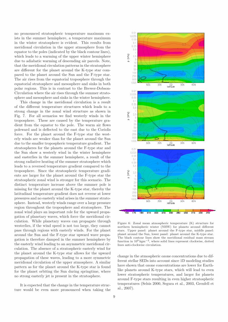
no pronounced stratospheric temperature maximum ex-ists in the summer hemisphere, a temperature maximumin the winter stratosphere is evident. This results frommeridional circulation in the upper atmosphere from theequator to the poles (indicated by the black contour lines),which leads to a warming of the upper winter hemispheredue to adiabatic warming of descending air parcels. Note,that the meridional circulation patterns in the stratosphereare different for the planet around the K-type star com-pared to the planet around the Sun and the F-type star.The air rises from the equatorial troposphere through theequatorial stratosphere and mesosphere and sinks in bothpolar regions. This is in contrast to the Brewer-Dobson-Circulation where the air rises through the summer strato-sphere and mesosphere and sinks in the winter hemisphere.

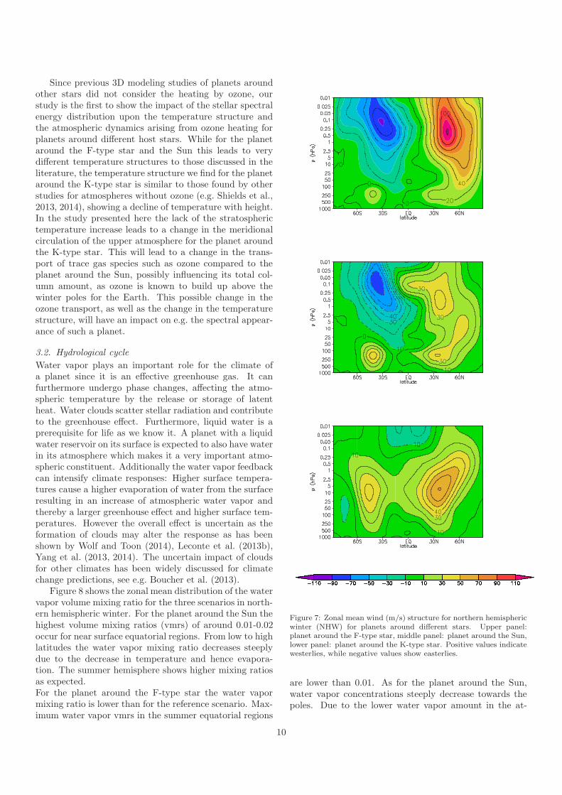
This change in the meridional circulation is a resultof the different temperature structures which leads to astrong change in the zonal wind structure as shown inFig. 7. For all scenarios we find westerly winds in thetroposphere. These are caused by the temperature gra-dient from the equator to the pole. The warm air flowspoleward and is deflected to the east due to the Coriolisforce. For the planet around the F-type star the west-erly winds are weaker than for the planet around the Sundue to the smaller tropospheric temperature gradient. Thestratospheres for the planets around the F-type star andthe Sun show a westerly wind in the winter hemisphereand easterlies in the summer hemisphere, a result of thestrong radiative heating of the summer stratosphere whichleads to a reversed temperature gradient compared to thetroposphere. Since the stratospheric temperature gradi-ents are larger for the planet around the F-type star thestratospheric zonal wind is stronger for this scenario. Thedistinct temperature increase above the summer pole ismissing for the planet around the K-type star, thereby thelatitudinal temperature gradient does not reverse at lowerpressures and no easterly wind arises in the summer strato-sphere. Instead, westerly winds range over a large pressureregion throughout the troposphere and stratosphere. Thezonal wind plays an important role for the upward propa-gation of planetary waves, which force the meridional cir-culation. While planetary waves can propagate throughwesterlies, if the wind speed is not too large, they cannotpass through regions with easterly winds. For the planetaround the Sun and the F-type star upward wave propa-gation is therefore damped in the summer hemisphere bythe easterly wind leading to an asymmetric meridional cir-culation. The absence of a stratospheric easterly wind forthe planet around the K-type star allows for the upwardpropagation of these waves, leading to a more symmetricmeridional circulation of the upper atmosphere. A similarpattern as for the planet around the K-type star is foundfor the planet orbiting the Sun during springtime, whereno strong easterly jet is present in the stratosphere.

It is expected that the change in the temperature struc-ture would be even more pronounced when taking the

Figure 6: Zonal mean atmospheric temperature (K) structure fornorthern hemispheric winter (NHW) for planets around differentstars. Upper panel: planet around the F-type star, middle panel:planet around the Sun, lower panel: planet around the K-type star.The black contour lines show the meridional residual mass streamfunction in 109 kgm−2, where solid lines represent clockwise, dottedlines anti-clockwise circulation.

change in the atmospheric ozone concentrations due to dif-ferent stellar SEDs into account since 1D modeling studieshave shown that ozone concentrations are lower for Earth-like planets around K-type stars, which will lead to evenlower stratospheric temperatures, and larger for planetsaround F-type stars resulting in even higher stratospherictemperatures (Selsis 2000, Segura et al., 2003, Grenfell etal., 2007).

9

Since previous 3D modeling studies of planets aroundother stars did not consider the heating by ozone, ourstudy is the first to show the impact of the stellar spectralenergy distribution upon the temperature structure andthe atmospheric dynamics arising from ozone heating forplanets around different host stars. While for the planetaround the F-type star and the Sun this leads to verydifferent temperature structures to those discussed in theliterature, the temperature structure we find for the planetaround the K-type star is similar to those found by otherstudies for atmospheres without ozone (e.g. Shields et al.,2013, 2014), showing a decline of temperature with height.In the study presented here the lack of the stratospherictemperature increase leads to a change in the meridionalcirculation of the upper atmosphere for the planet aroundthe K-type star. This will lead to a change in the trans-port of trace gas species such as ozone compared to theplanet around the Sun, possibly influencing its total col-umn amount, as ozone is known to build up above thewinter poles for the Earth. This possible change in theozone transport, as well as the change in the temperaturestructure, will have an impact on e.g. the spectral appear-ance of such a planet.

3.2. Hydrological cycle

Water vapor plays an important role for the climate ofa planet since it is an effective greenhouse gas. It canfurthermore undergo phase changes, affecting the atmo-spheric temperature by the release or storage of latentheat. Water clouds scatter stellar radiation and contributeto the greenhouse effect. Furthermore, liquid water is aprerequisite for life as we know it. A planet with a liquidwater reservoir on its surface is expected to also have waterin its atmosphere which makes it a very important atmo-spheric constituent. Additionally the water vapor feedbackcan intensify climate responses: Higher surface tempera-tures cause a higher evaporation of water from the surfaceresulting in an increase of atmospheric water vapor andthereby a larger greenhouse effect and higher surface tem-peratures. However the overall effect is uncertain as theformation of clouds may alter the response as has beenshown by Wolf and Toon (2014), Leconte et al. (2013b),Yang et al. (2013, 2014). The uncertain impact of cloudsfor other climates has been widely discussed for climatechange predictions, see e.g. Boucher et al. (2013).

Figure 8 shows the zonal mean distribution of the watervapor volume mixing ratio for the three scenarios in north-ern hemispheric winter. For the planet around the Sun thehighest volume mixing ratios (vmrs) of around 0.01-0.02occur for near surface equatorial regions. From low to highlatitudes the water vapor mixing ratio decreases steeplydue to the decrease in temperature and hence evapora-tion. The summer hemisphere shows higher mixing ratiosas expected.For the planet around the F-type star the water vapormixing ratio is lower than for the reference scenario. Max-imum water vapor vmrs in the summer equatorial regions

Figure 7: Zonal mean wind (m/s) structure for northern hemisphericwinter (NHW) for planets around different stars. Upper panel:planet around the F-type star, middle panel: planet around the Sun,lower panel: planet around the K-type star. Positive values indicatewesterlies, while negative values show easterlies.

are lower than 0.01. As for the planet around the Sun,water vapor concentrations steeply decrease towards thepoles. Due to the lower water vapor amount in the at-

10

mosphere the greenhouse effect becomes less efficient, asindicated by the more negative near surface values of thenet thermal radiation in Fig. 4.

For the Earth-like planet around the K-type star muchhigher water vapor mixing ratios are obtained than for theplanet around the Sun, reaching vmrs higher than 0.12in the equatorial region near the surface. Mixing ratiostypical for the surface of the Earth occur at much higheraltitudes at pressures of about 100-200hPa. Here the con-centrations are nearly constant over all latitudes, which re-sults from a change in the hydrological cycle, which leadsto recycling of water in the upper atmosphere. Whilefor the Earth, cloud formation and precipitation lead toefficient replenishment of surface water, Figure 9 showsthat for the planet around the K-type star a large partof the precipitation evaporates or melts before reachingthe planetary surface. The high atmospheric temperatureslead to melting of all solid precipitation at pressures largerthan 200 hPa. The amount of water recycled by this melt-ing and evaporation processes in the upper atmosphereconstitutes a reservoir larger than the precipitation reach-ing the surface for the planet around the Sun. Neverthelessrainfall at the surface is intensified on the planet aroundthe K-type star compared to the reference scenario. Thus,these high water vapor concentrations are the result of achange in the water vapor feedback cycle and the hydro-logical cycle.The high water vapor mixing ratios for the planet aroundthe K-type star are also a result of the assumed land-seamask, as about 70% of the planet assumed is covered withwater. For a planetary scenario with a much smaller wa-ter reservoir, e.g. a planet without any ocean, the impactof the hydrological cycle upon surface temperatures wouldbe much smaller as discussed e.g. by Abe et al. (2011),since the greenhouse effect of water vapor would be muchweaker in such a scenario. For a planetary scenario witha larger ocean reservoir, we expect a similar response ofthe hydrological cycle as the amount of water vapor in theatmosphere is related to the surface temperature via phaseequilibrium. Due to a lower surface albedo for an oceanplanet, surface temperatures would probably be higher.

A comparison of the water vapor concentrations forthe planet around the K-type star with model results ofKasting et al. (1993), who investigated the water loss limitas an inner boundary of the habitable zone shows that thestratospheric water vapor vmr (ca. 2×10−4 ) is still belowtheir critical value of 3×10−3 . Thus, according to these re-sults a water reservoir of one Earth ocean should be stableover 4.5Gyrs when considering diffusion limited escape ofhydrogen to space for this scenario. Kasting and Pollack(1983) however calculated atmospheric concentrations inthe upper atmosphere of a Venus-like terrestrial planet,starting with stratospheric water vapor concentrations sim-ilar to those obtained here and found that an increase inthe solar EUV flux by a factor of ten may result in stronghydrogen escape. Therefore, it is possible that even though

the water vapor concentrations are below the critical valuecalculated by Kasting et al. (1993) a different stellar spec-tral energy distribution, especially with increased high-energy radiation may still lead to a water loss for such ascenario.

Figure 8: Zonal mean distribution of water vapor (vmr) for plan-ets around different stars in NHW. Upper panel: results for planetaround the F-type star, middle panel: planet around the Sun, lowerpanel: planet around the K-type star. Note the linear pressure scale.

In addition to water vapor, also clouds can have astrong impact on exoplanetary climate as shown e.g. byKitzmann et al. (2010). We cannot judge whether the for-

11

Figure 9: Global orbital mean rain and snowfall for Earth-like planetsaround different stars. The left panel shows the rainfall profile andthe right panel the vertical snowfall profile. The planet around theF-type star is depicted in blue, the planet around the Sun in black,and the planet around the K-type star in red.

mation of clouds in Earth-like atmospheres of rocky extra-solar planets is captured by the cloud scheme included inour 3D model, since even for Earth climate predictions theimpact of clouds varies over a wide range (Boucher et al.,2013). A first step towards the understanding of the cloudfeedback for rocky extrasolar planets could be a modelcomparison for such scenarios. For the planet around theF-type star we find an increase in cloud cover and a de-crease in cloud cover for the planet around the K-type starcompared to the planet around the Sun, see also table 2.We find the same behavior for the water ice column. Forthe cloud water column however we find an increase forthe planet around the K-type star and a decrease for theplanet around the F-type star, see table 2. The cloud wa-ter column is about twice as high for the planet aroundthe K-type star compared to the planet around the Sun.The greenhouse effect caused by clouds (Cloud GHE intable 2) is calculated from the difference in surface tem-perature and the effective temperature from the longwaveradiation of the planets for cloudy and clear sky condi-tions. Our results suggest the cloud GHE is larger forthe planet around the K and the F-type star than for theplanet around the Sun. This indicates that the influenceof clouds critically depends on cloud properties and at-mospheric temperatures, and cannot be easily estimatedwithout sophisticated cloud modeling. The differences incloud impact of different Earth climate models upon Earthclimate predictions, but also studies of exoplanet scenarios,such as e.g. Wolf and Toon (2014); Leconte et al. (2013b),show that much more work is needed to understand thebehavior and influence of clouds for the Earth and for ex-oplanetary climates. For the planet around the K-typestar, the cloud GHE constitutes only about 15% of thetotal GHE, while for the planet around the F-type starit is about 43% and 22% for the planet around the Sun.Hence, for the warm scenario the cloud GHE seems to beof minor importance.

3.3. Surface conditions

The change in temperature is linked to a change in the sur-face albedo via the albedo feedback. Higher temperatureslead to melting of sea ice whereas lower temperatures willlead to its buildup. Figure 10 shows the zonal orbital meansurface albedo for the three scenarios studied. At low andmid latitudes the albedo is the same for all scenarios. Atmid to high latitudes the albedo differs depending on snowand ice coverage.For the planet around the K-type star no sea ice or snowis present, leading to a uniformly low surface albedo.The highest albedos occur for the planet around the F-typestar at the north pole, which is a result of strong buildupof sea ice. In the southern hemisphere highest albedos oc-cur also for the planet around the F-type star at latitudeswhere sea ice is present.

For the planet around the F-type star the ice-albedofeedback causes an increase in surface albedo due to buildupof sea ice down to latitudes of about 40◦. Despite the factthat water vapor concentrations are low, i.e. the green-house effect of water is smaller than for the planet aroundthe Sun, the increase in surface albedo is not large enoughto cause a runaway glaciation. Note however, that de-pending on the stellar SED, the effect of the surface albedomay differ, since especially the albedo of snow is stronglywavelength-dependent, as e.g. shown by Joshi and Haberle(2012). In our study we do not account for the wavelengthdependence of the surface albedo. Including it may in-crease the ice-albedo feedback for the planet around theF-type star as shown by Shields et al. (2013).

Figure 10: Zonal orbital mean surface albedo for planets arounddifferent stars. The planet around the F-type star is depicted inblue, the planet around the Sun in black, and the planet around theK-type star in red.

3.4. Sensitivity tests

For an extrasolar planet, besides many other parameters,also the oceanic heat flux term is a-priori unknown. Itwas shown, by e.g. Yang et al. (2013), Hu and Yang (2013)and Cullum et al. (2014), that the oceanic heat flux may

12

strongly influence atmospheric GCM results and surfacetemperatures. Therefore, we test the sensitivity of ourmodel results to a change in the q-flux term. Additionally,we vary the orbital period to estimate its influence on themodel results, since different lengths in season may leadto different results due to the large thermal inertia of theocean.The scenarios and their resulting global orbital mean tem-perature are summarized in table 3. Overall, the differencein temperature due to different orbital periods is small,about 1K for the planet around the F-type star (compar-ing scenarios F3D and F3Dq4, which both use the q4 q-fluxbut different orbital periods). However, the seasonalitychanges, hence for longer orbital periods, longer temper-ature maxima and minima are obtained, see Fig. 11. Forthe planet around the F-type star and the Sun the season-ality is more pronounced than for the planet around theK-type star. While for the planet around the K-type starthe atmosphere is dominated by the large amount of watervapor, for the planet around the F-type star and the Sunthe build-up and melting of sea ice are important factorsfor the seasonal temperature variability. Note that for theplanet around the F-type star we conducted most of thesensitivity tests with an orbital period of 450 days, whichwas computationally less expensive than using the physi-cally correct orbital period of 868 days used for the resultsin the previous sections .

The influence of varying the oceanic heat flux (q-flux),used in the mixed layer ocean model to calculate the seasurface temperatures and sea ice, is a little larger, lead-ing to a temperature difference of up to 2K for moderatechanges in the q-flux term. This term partly representsthe oceanic circulation and heat transport. We appliedfive different q-flux terms q1-q5, as described in sec. 2.3.Figure 11 suggests that moderately varying the q-flux term(shown are q2-q4) does not change the global temperatureresponse. A seasonal variation of the temperature can beidentified for the planet around the Sun and the F-typestar. For the planet around the K-type star the the varia-tion of the temperature is less pronounced. A larger vari-ability at smaller timescales is visible which is less periodic.This is caused by the large amount of water compoundsin the atmosphere which are highly variable on timescalessmaller than the seasons.

While on the global scale the near surface temperaturesdeviate by up to 10K for different q-fluxes and orbital pe-riods (except for the planet around the F-type star witha q-flux of 0), on the regional scale the temperature dif-ferences are larger. For the planet around the F-type starwe find a temperature difference of about 30-50K at thesummer pole and of about 20K for the winter pole dueto the difference in orbital period, with higher tempera-tures in summer and lower temperatures in winter for thelonger orbital period (not shown). For the planet aroundthe Sun the different q-fluxes q1-q3 lead to a small changein the global annual mean near surface temperatures from

an exoplanet perspective. For Earth climate calculationsthese differences of about 2K are however large. On thelocal scale we find e.g. larger near surface temperatures (ofabout 5K) above the equatorial ocean and the southernpole for the q-flux q3. The zonal seasonal mean tempera-ture structures are not influenced strongly by the changeof the orbital periods or q-fluxes either, from an exoplanetperspective. Compared with the scenarios with an orbitalperiod of 365 days and the q-flux q1 we find a very simi-lar temperature structure, hydrological cycle, and a simi-lar dynamical behavior, and surface response compared tothose presented in the previous sections. It was not antici-pated that the change in the orbital period and the oceanicheat flux would have such a small effect on the mean 3Dmodel results.

Only the assumption of an extreme and unrealistic q-flux of zero (q5) leads to a strong change in surface condi-tions for the planet around the F-type star, which under-goes global glaciation. Hence, for this scenario, an oceanicheat flux is required to prevent the planet from freezingcompletely. For the planet around the K-type star theorbital mean temperature only decreases by about 5K forthe q5 q-flux, since the greenhouse effect of the atmospheredominates the heat budget.In Shields et al. (2013) a similar scenario has been studied:an Earth-like planet around an F-type star with an oceanicheat flux of zero. They discuss that their planet is closeto global glaciation for a total amount of incoming stellarradiation as Earth receives from the Sun. Hence, althoughthey include a wavelength-dependent ice albedo in theirstudy, which should enhance the response by increasedscattering of stellar light, in their model calculations theplanet does not undergo global glaciation. Their model re-sults differ from ours because they disregard ozone in theircalculations and assume a surface completely covered withwater which lowers the background surface albedo. Fur-thermore, the albedo they assume in the visible wavelengthregime (0.8 cold dry snow) is about equal to the one weassume in our model calculations for the entire shortwaveregime (0.8 for snow on ice). Their albedo in the NIRregime is however lower (0.68 for snow on ice). Addition-ally, from their paper it is unclear whether they also usedifferent amounts of greenhouse gases, such as CO2 andCH4, which may also yield higher surface temperatures.

3.5. Comparison of the 3D to the 1D model results

To evaluate the habitability of rocky extrasolar planets1D atmospheric models are often utilized since the 1D as-sumption keeps the number of boundary conditions small.Furthermore, in future, averaged quantities of these dis-tant worlds will be the first to be retrieved. However, ithas been suggested that for rocky extrasolar planets closeto the inner edge of the habitable zone 3D phenomenamay have to be taken into account for certain scenariosof e.g. tidally-locked extrasolar planets or for planets withsmall water reservoirs (Abe et al., 2011, Leconte et al.,

13

Table 3: Sensitivity test scenarios and global orbital mean near-surface temperatures.

Scenario Star (stellar type) orbital period (d) q-flux term (variability) T2m (K)

F3D σ Boo (F2V) 868.64 q4 (am) 273.6F3Dq0 σ Boo (F2V) 450.0 q5 (=0) 234.0F3Dq4 σ Boo (F2V) 450.0 q4 (am) 274.7F3Dq3 σ Boo (F2V) 450.0 q3 (mm) 275.5F3Dq2 σ Boo (F2V) 450.0 q2 275.2F3Dq1 σ Boo (F2V) 365.25 q1 275.0Sun3D Sun (G2V) 365.25 q2 288.6Sun3Dq3 Sun (G2V) 365.25 q3 (mm) 289.7Sun3Dq1 Sun (G2V) 365.25 q1 287.7K3D ǫ Eri (K2V) 184.00 q2 334.9K3Dq0 ǫ Eri (K2V) 184.00 q5 (=0) 329.2K3Dq2 ǫ Eri (K2V) 184.00 q3 (mm) 336.2K3Dq1 ǫ Eri (K2V) 365.25 q1 334.5

Figure 11: Influence of different q-fluxes and orbital periods on near-surface temperature for planets around different stars. Results forthe planet around the F-type star in blue, for solar radiation in black,and for the planet around the K-type star in red. q-flux corrections:q1 dot-dot dashed, q2 solid, q3 long dashed, q4 dot-dashed for theF3Dq4 scenario with a 450 days orbit, q4 long dashed-short dashedfor the F3D scenario with a 868 days orbit, q5 dotted.

2013b, Yang et al., 2014).

Here we test whether 3D phenomena need to be takeninto account for habitable Earth-like extrasolar planetswhich are not tidally locked by comparing the global or-bital mean results of the 3D model with those of a steady-state radiative-convective model (see section 2.2). The up-per panel in Fig. 12 shows the temperature-pressure pro-files for the three scenarios as computed with the 3D andthe 1D models.

For the planets around the Sun and around the F-typestar, the temperature profiles compare well for pressuresbetween 1000hPa and ≈1 hPa. Differences at larger heightmay be explained by the different model regimes. In par-

ticular, the 3D model extends to 0.01 hPa while the 1Dmodel only ranges to 0.066hPa. Also in the 1D model,e.g. the absorption of radiation at 121.5 nm (Lyman α) bymolecular oxygen is not considered leading to lower tem-peratures in the upper model atmosphere. For the planetaround the K-type star a larger difference between theglobal orbital mean profile of the 3D model calculationsand the 1D model can be found. This mainly results fromthe large difference in the calculated water vapor profiles,which are shown in the lower panel of Fig. 12. In the1D model the water vapor profile is determined from anassumed vertical profile of relative humidity. For the 1Dmodel calculations shown in Fig. 12 (F1D, Sun1D, K1D)a relative humidity profile as measured for present Earth(Manabe and Wetherald, 1967) is assumed for the calcu-lation of the water vapor profile, which starts with a rel-ative humidity of 77% at the surface and then decreasesthroughout the troposphere. This results in the steep de-cline with height of water vapor in the atmospheres ascalculated by the 1D model. However, in the 3D modelcalculations, as shown in section 3.2, the distribution ofwater vapor in the atmosphere differs due to a change inthe hydrological cycle. Therefore, the water vapor profileand thus also the temperature profiles as well as the globalmean surface values (Tab. 4) calculated by the 1D and the3D model disagree for the planet around the K-type star.

To test whether the 3D global orbital mean profiles cannevertheless be approximated by the 1D model, we addi-tionally compared the 3D model results for the K-type starwith 1D model profiles calculated with a relative humidityof 100% by Stracke (2012) (K1DRH100). This study uti-lized the same atmospheric model however with e.g. animproved thermal radiative transfer scheme (applicableto larger temperature and pressure range, von Paris et al.(2010)), and applied it to an Earth-like planet around dif-ferent types of stars however neglecting the influence of

14

0.01

0.1

1

10

100

1000 150 200 250 300 350 400

p (h

Pa)

T (K)

0.01

0.1

1

10

100

1000 1e-06 1e-05 0.0001 0.001 0.01 0.1 1

p (h

Pa)

vmr H2O

Figure 12: Mean temperature (top) and water vapor (bottom) pro-files for Earth-like planets around different types of stars. Globalorbital mean results from the 3D model in solid, profiles from the1D model in dashed lines. Results the planet around the F-type starin blue, for solar radiation in black, and for the planet around theK-type star in red.

Table 4: 1D and 3D global mean temperature (T) and watervapor vmr (H2O) at 1000 hPa for the Earth-like planets arounddifferent stars as calculated in this study, Star1D/3D, and inStracke (2012) with different relative humidity profiles: RHMW fromManabe and Wetherald (1967) RH100 with a relative humidity of100%.

Scenario T (K) H2O (%)

F3D 274.3 0.6F1D 280.1 0.8Sun3D 289.0 1.4Sun1D 287.7 1.3K3D 333.4 15.6K1D 292.9 1.7K1DRHMW 292.0 1.7K1DRH100 329.0 14.1

oxygen, ozone, methane, and nitrous oxide. For thesemodel calculations (K1DRHMW, K1DRH100) a surfacealbedo of 0.22 was assumed. As can be inferred fromFig. 13, for the assumption of a fully saturated atmosphere

(K1DRH100) the tropospheric profiles of the 3D model re-sults for the planet around the K-type star and 1D modelcalculation from Stracke (2012) agree well. Surface tem-peratures and water vapor volume mixing ratios also com-pare better for this assumption, see table 4.

10

100

1000 100 150 200 250 300 350 400

p (h

Pa)

T (K)

Figure 13: Comparison of the global orbital mean tropospheric tem-perature profile of the 3D model results for the planet around theK-type star (red, solid) with 1D model results (Stracke, 2012) forthe corresponding scenario with different RH profiles: orange, dottedwith a relative humidity profile from Manabe and Wetherald (1967),green, short-dashed with a relative humidity of 100%

This implies that the 1D model can indeed approximatethe global orbital mean climate states calculated with the3D model, when assuming an appropriate relative humid-ity profile. Note, that assuming a relative humidity of100% in the 1D model increases the surface temperatureof the planet around the Sun to 305K (for an atmospherewith N2, CO2, and H2O). Thus the agreement of the 3Dand 1D model results strongly depends on the choice ofthe relative humidity profile used for the water vapor pro-file calculation. Which profile to choose is however a-prioriunknown.

Note that the realization of a global mean relative hu-midity of 100% seems unlikely as atmospheric dynamicswill lead to drying of air during ascent (Leconte et al.,2013a), by condensation and cloud formation for most sce-narios. In the 3D model calculations presented in sec. 3.1–3.3 we find a global mean surface relative humidity ofonly 74% for the planet around the K-type star (71%for the planet around the Sun and 69% for the planetaround the F-type star), lower than the relative humid-ity of 100% assumed in the 1D model to find a goodagreement between the results. However, the decreasein relative humidity with height is weaker for the planetaround the K-type star than for the planet around theSun and the F-type star in the 3D model results. Forthese cooler scenarios the decrease is similar to the RHprofile by Manabe and Wetherald (1967) assumed in the1D model. Including the global mean relative humidity

15

profile from the 3D model calculations in the 1D modelresults in an increased surface temperature which reaches315K. We find a similar good agreement between the 1Dand 3D model results as with a constant RH of 100% inthe 1D model, when assuming a fixed water vapor profilecorresponding to the 3D global mean water vapor profileand a global mean surface albedo of 0.1 in the 1D modelcalculations for the planet around the K-type star, yield-ing a surface temperature of 328K.

From our 3Dmodel calculations which include the changein the hydrological cycle, the water vapor feedback, andthe ice-albedo feedback, we deduce a maximum differencein the global orbital mean near-surface temperature of61K, for the planet around the F-type star and the planetaround the K-type star (see table 4) when including anEarth-like oceanic heat transport. Including also the q-fluxsensitivity test scenarios (see section 3.4) the maximumdifference is 102K for the same amount of total energyincident at top of the atmosphere. The largest differencein near surface temperatures obtained by the 1D modelcalculations in this work is 49K, for the planet aroundthe F-type star with a relative humidity profile followingManabe and Wetherald (1967) and the planet around theK-type star with a relative humidity of 100%. The maxi-mum temperature difference obtained by the 1D model cal-culations is smaller because a change in the surface albedois not captured by the 1D model calculations. Note thatthe 3D model results depend on complex parameteriza-tions which are adjusted to reproduce present and pastEarth climates. Therefore, the results may differ in ab-solute numbers for varying the parameter sets and modelcodes. Our results should hence be considered to be ofmore of a qualitative than of quantitative nature.

In 1D model studies, similar to that presented here, thesurface albedo is often tuned to fit the mean temperatureof the Earth (288K), and therefore not only includes thereal surface albedo, but additionally mimics the reflectiv-ity of clouds within the atmosphere. The surface albedo inthe 3D model is calculated and differs for the scenarios in-vestigated here as discussed in section 3.3. As long as theplanets stay habitable the difference in surface albedo ishowever relatively small (∆albedo ∼ 0.1). When includingthe sensitivity scenario where the planet around the F-typestar undergoes global glaciation the difference in albedo islarge (∆albedo ∼ 0.5). The impact of clouds on the plan-etary albedo can be very diverse (see e.g. Kitzmann et al.,2010), and therefore difficult to capture.

Which surface albedo is realized for a certain plan-etary scenario needs to be calculated interactively by acoupled 3D atmosphere-ocean general circulation model(AOGCM), since the resulting surface albedo strongly de-pends on the oceanic heat transport as illustrated in sec-tion 3.4. Therefore atmospheric GCMs coupled to a mixedlayer ocean, as utilized in this work, may only give afirst estimate of the surface albedo for a certain planetaryscenario. It would preferably be calculated with coupled

atmosphere-ocean models. Such calculations will howeverintroduce an even larger amount of parameters which areunknown for extrasolar planets, and are more expensivein terms of computing time. Their impact should never-theless be explored. It should be noted that the planetarysurface albedo is important to deduce the climate of plan-ets with relatively thin atmospheres, as for these planetsit has large impact on the energy budget. For planetswith thicker atmospheres e.g. at the inner edge of thehabitable zone, where one may expect water dominatedatmospheres (e.g. Stracke, 2012) or at the outer edge ofthe habitable zone where one may expect thick CO2-do-minated atmospheres its impact is much smaller becauseit is masked by the thick atmospheres (von Paris et al.,2013b; Shields et al., 2013) .

4. Summary and conclusion

The results of 3D GCM climate modeling of Earth-likeplanets around F, G, and K-type stars have been dis-cussed in this paper. It has been shown that differentstellar spectral energy distributions may lead to very dif-ferent climate states of an Earth-like planet for the sametotal amount of stellar energy incident at the top of theatmosphere. This results from the wavelength-dependentabsorption and scattering properties of the atmosphere,and an amplification of the climate response by positiveclimate feedback cycles, namely the water vapor and theice-albedo feedback.For the planet around the F-type star we find an enhancedheating of the stratosphere by ozone due to the changein the stellar energy distribution compared to the planetaround the Sun. For the planet around the K-type star wefind a strong change in the vertical temperature structurewith no temperature increase in the stratosphere, causedby decreased heating by ozone absorption, and a change inthe hydrological cycle due to the high tropospheric tem-peratures. For nearly all scenarios studied, the Earth-likeplanets result in habitable surface conditions. Only whenneglecting the (parametrized) oceanic heat transport forthe planet around the F-type star, which is rather un-physical, we find uninhabitable surface conditions. Forthis scenario the planet undergoes global glaciation. Amoderate change in the oceanic heat flux term and in theorbital period do not show a strong impact on the meanplanetary surface climate.Comparing the global orbital mean of the 3D model re-sults to those of a cloud-free 1D radiative-convective col-umn model showed that the temperature response maybe approximated by the 1D model. The agreement of theresults, however, crucially depends on the choice of the rel-ative humidity profile utilized to calculate the water vaporprofile.

16

Acknowledgments

We thank the anonymous referees for their helpful com-ments on the manuscript. This work has been partlysupported by the Forschungsallianz Planetary Evolution

and Life and the Postdoc Program ”Atmospheric dynam-ics and Photochemistry of Super Earth planets” of theHelmholtz Gemeinschaft (HGF). This study has partlyreceived financial support from the French State in theframe of the ”Investments for the future” Programme IdExBordeaux, reference ANR-10-IDEX-03-02. The 3D modelcalculations have been performed on the North-GermanSupercomputing Alliance (HLRN) parallel supercomput-ing system. We would like to thank S. Dietmuller andM. Ponater for providing and advising us with the mixedlayer ocean.

References

Abe, Y., Abe-Ouchi, A., Sleep, N. H., Zahnle, K. J., Jun. 2011.Habitable Zone Limits for Dry Planets. Astrobiology 11, 443–460.

Batalha, N. M., Borucki, W. J., Bryson, S. T., Buchhave, L. A.,Caldwell, D. A., Christensen-Dalsgaard, J., Ciardi, D., Dunham,E. W., Fressin, F., Gautier, III, T. N., and 42 coauthors, Mar.2011. Kepler’s First Rocky Planet: Kepler-10b. AstrophysicalJournal 729, 27.

Bechtold, P., Chaboureau, J.-P., Beljaars, A., Betts, A. K., Kohler,M., Miller, M., Redelsperger, J.-L., 2004. The simulation of the di-urnal cycle of convective precipitation over land in a global model.Q. J. R. Meteorol. Soc. 130, 3119–3137.

Boucher, O., Randall, D., Artaxo, P., Bretherton, C., Feingold, G.,Forster, P., Kerminen, V.-M., Kondo, Y., Liao, H., Lohmann, U.,Rasch, P., Satheesh, S., Stevens, S. S. B., Zhang, X., 2013. Cloudsand aerosols. In: Stocker, T., Qin, D., Plattner, G.-K., Tignor,M., Allen, S., Boschung, J., Nauels, A., Xia, Y., Bex, V., Midg-ley, P. (Eds.), Climate Change 2013: The Physical Science Basis.Contribution of Working Group I to the Fifth Assessment Reportof the Intergovernmental Panel on Climate Change. CambridgeUniversity Press, pp. 571–657.

Boyajian, T. S., McAlister, H. A., van Belle, G., Gies, D. R., tenBrummelaar, T. A., von Braun, K., Farrington, C., Goldfinger,P. J., O’Brien, D., Parks, J. R., Richardson, N. D., Ridgway, S.,Schaefer, G., Sturmann, L., Sturmann, J., Touhami, Y., Turner,N. H., White, R., Feb. 2012. Stellar Diameters and Temperatures.I. Main-sequence A, F, and G Stars. Astrophysical Journal 746,101.

Brinkop, S., Roeckner, E., Mar. 1995. Sensitivity of a general circu-lation model to parameterizations of cloud turbulence interactionsin the atmospheric boundary layer. Tellus Series A 47, 197.

Butler, R. P., Wright, J. T., Marcy, G. W., Fischer, D. A., Vogt,S. S., Tinney, C. G., Jones, H. R. A., Carter, B. D., Johnson,J. A., McCarthy, C., Penny, A. J., Jul. 2006. Catalog of NearbyExoplanets. Astrophysical Journal 646, 505–522.

Charbonneau, D., Berta, Z. K., Irwin, J., Burke, C. J., Nutzman,P., Buchhave, L. A., Lovis, C., Bonfils, X., Latham, D. W., Udry,S., Murray-Clay, R. A., Holman, M. J., Falco, E. E., Winn, J. N.,Queloz, D., Pepe, F., Mayor, M., Delfosse, X., Forveille, T., Dec.2009. A super-Earth transiting a nearby low-mass star. Nature462, 891–894.

Charnay, B., Forget, F., Wordsworth, R., Leconte, J., Millour, E.,Codron, F., Spiga, A., Sep. 2013. Exploring the faint young Sunproblem and the possible climates of the Archean Earth with a3-D GCM. Journal of Geophysical Research (Atmospheres) 118,10414.

Cullum, J., Stevens, D., Joshi, M., Aug. 2014. The Importance ofPlanetary Rotation Period for Ocean Heat Transport. Astrobiol-ogy 14, 645–650.

Dumusque, X., Bonomo, A. S., Haywood, R. D., Malavolta, L.,Segransan, D., Buchhave, L. A., Collier Cameron, A., Latham,D. W., Molinari, E., Pepe, F., Udry, S., Charbonneau, D.,Cosentino, R., and 21 Co-authors, Jul. 2014. The Kepler-10 Plan-etary System Revisited by HARPS-N: A Hot Rocky World and aSolid Neptune-Mass Planet. Astrophysical Journal 789, 154.

Flato, G., Marotzke, J., Abiodun, B., Braconnot, P., Chou, S.,Collins, W., Cox, P., Driouech, F., Emori, S., Eyring, V., For-est, C., Gleckler, P., Guilyardi, E., Jakob, C., Kattsov, V., Rea-son, C., Rummukainen, M., 2013. Evaluation of Climate Models.In: Stocker, T., Qin, D., Plattner, G.-K., Tignor, M., Allen, S.,Boschung, J., Nauels, A., Xia, Y., Bex, V., Midgley, P. (Eds.),Climate Change 2013: The Physical Science Basis. Contributionof Working Group I to the Fifth Assessment Report of the In-tergovernmental Panel on Climate Change. Cambridge UniversityPress, Cambridge, United Kingdom and New York, NY, USA, pp.741–866.

Forget, F., 1998. Habitable Zone around other Stars. Earth Moonand Planets 81, 59–72.

Fortuin, J., Kelder, H., Dec. 1998. An ozone climatology based onozonesonde and satellite measurements. Journal of Geophysics Re-search 103, 31709–31734.

Fouquart, Y., Bonnel, B., 1980. Computations of solar heating of theearth’s atmosphere: A new parameterization. Beitrage zur Physikder Atmosphare 53, 35–62.

Grenfell, J. L., Stracke, B., von Paris, P., Patzer, B., Titz, R., Segura,A., Rauer, H., 2007. The response of atmospheric chemistry onearthlike planets around F, G and K stars to small variations inorbital distance. Planetary and Space Science 55 (5), 661–671.

Gueymard, C. A., April 2004. The sun’s total and spectral irradiancefor solar energy applications and solar radiation models. SolarEnergy 76 (4), 423–453.

Hagemann, S., 2002. ”an improved land surface parameter datasetfor global and regional climate models”. Tech. rep., Max-Planck-Institut fur Meteorologie.

Hart, M. H., Jan. 1979. Habitable Zones about Main Sequence Stars.Icarus 37, 351–357.

Hedelt, P., von Paris, P., Godolt, M., Gebauer, S., Grenfell, J. L.,Rauer, H., Schreier, F., Selsis, F., Trautmann, T., May 2013.Spectral features of Earth-like planets and their detectability atdifferent orbital distances around F, G, and K-type stars. Astron-omy and Astrophysics 553, A9.

Hu, Y., Yang, J., 2013. Role of ocean heat transport in climates oftidally locked exoplanets around M dwarf stars. In: Proceedings ofthe National Academy of Sciences of the United States of America.Vol. 111. pp. 1–6.

Jockel, P., Tost, H., Pozzer, A., Brul, C., Buchholz, J., Ganzeveld, L.,Hoor, P., Kerkweg, A., Lawrence, M., Sander, R., Steil, B., Stiller,G., Tanarhte, M., Taraborrelli, D., van Aardenne, J., Lelieveld,J., 2006. The atmospheric chemistry general circulation modelecham5/messy1: consistent simulation of ozone from the surfaceto the mesosphere. Atmospheric Chemistry and Physics 6 (12),5067–5104.

Joshi, M., Jun. 2003. Climate Model Studies of Synchronously Ro-tating Planets. Astrobiology 3, 415–427.

Joshi, M. M., Haberle, R. M., Jan. 2012. Suppression of the Water Iceand Snow Albedo Feedback on Planets Orbiting Red Dwarf Starsand the Subsequent Widening of the Habitable Zone. Astrobiology12, 3–8.

Joshi, M. M., Haberle, R. M., Reynolds, R. T., Oct. 1997. Simula-tions of the Atmospheres of Synchronously Rotating TerrestrialPlanets Orbiting M Dwarfs: Conditions for Atmospheric Collapseand the Implications for Habitability. Icarus 129, 450–465.

Kasting, J. F., Pollack, J. B., Mar. 1983. Loss of water from Venus.I - Hydrodynamic escape of hydrogen. Icarus 53, 479–508.

Kasting, J. F., Whitmire, D. P., Reynolds, R. T., Jan. 1993. Habit-able Zones around Main Sequence Stars. Icarus 101, 108–128.

Kitzmann, D., Patzer, A. B. C., von Paris, P., Godolt, M., Stracke,B., Gebauer, S., Grenfell, J. L., Rauer, H., Feb. 2010. Clouds inthe atmospheres of extrasolar planets. I. Climatic effects of multi-layered clouds for Earth-like planets and implications for habitable

17

zones. Astronomy and Astrophysics 511, A66+.Kopparapu, R. K., Ramirez, R., Kasting, J. F., Eymet, V., Robin-

son, T. D., Mahadevan, S., Terrien, R. C., Domagal-Goldman, S.,Meadows, V., Deshpande, R., Mar. 2013. Habitable Zones aroundMain-sequence Stars: New Estimates. Astrophysical Journal 765,131.

Kunze, M., Godolt, M., Langematz, U., Grenfell, J., Hamann-Reinus, A., Rauer, H., August 2014. Investigating the early Earthfaint young Sun problem with a general circulation model. Plan-etary and Space Science 98, 77–92.

Laursen, L., Eliasen, E., Oct. 1989. On the effects of the dampingmechanisms in an atmospheric general circulation model. TellusSeries A 41, 385–400.

Leconte, J., Forget, F., Charnay, B., Wordsworth, R., Pottier, A.,Dec. 2013a. Increased insolation threshold for runaway greenhouseprocesses on Earth-like planets. Nature 504, 268–271.

Leconte, J., Forget, F., Charnay, B., Wordsworth, R., Selsis, F.,Millour, E., Spiga, A., Jun. 2013b. 3D climate modeling of close-in land planets: Circulation patterns, climate moist bistability,and habitability. Astronomy and Astrophysics 554, A69.

Leger, A., Rouan, D., Schneider, J., Barge, P., Fridlund, M., Samuel,B., Ollivier, M., Guenther, E., Deleuil, M., Deeg, H. J., and151 coauthors, Oct. 2009. Transiting exoplanets from the CoRoTspace mission. VIII. CoRoT-7b: the first super-Earth with mea-sured radius. Astronomy and Astrophysics 506, 287–302.

Lohmann, U., Roeckner, E., Jun. 1996. Design and performance of anew cloud microphysics scheme developed for the ECHAM generalcirculation model. Climate Dynamics 12, 557–572.

Manabe, S., Wetherald, R. T., May 1967. Thermal Equilibrium ofthe Atmosphere with a Given Distribution of Relative Humidity.Journal of Atmospheric Sciences 24, 241–259.

Mlawer, E. J., Taubman, S. J., Brown, P. D., Iacono, M. J., Clough,S. A., Jul. 1997. Radiative transfer for inhomogeneous atmo-spheres: RRTM, a validated correlated-k model for the longwave.Journal of Geophysical Research 102, 16663–16682.

Nissen, K. M., Matthes, K., Langematz, U., Mayer, B., 2007. To-wards a better representation of the solar cycle in general circu-lation models. Atmospheric Chemistry and Physics 7 (20), 5391–5400.

Pierrehumbert, R., Gaidos, E., Jun. 2011. Hydrogen GreenhousePlanets Beyond the Habitable Zone. Astrophysical Journal Let-ters 734, L13.

Rauer, H., Gebauer, S., von Paris, P., Cabrera, J., Godolt, M., Gren-fell, J. L., Belu, A., Selsis, F., Hedelt, P., Schreier, F., May 2011.Potential biosignatures in super-Earth atmospheres. I. Spectralappearance of super-Earths around M dwarfs. Astronomy and As-trophysics 529, A8+.

Roeckner, E., Brokopf, R., Esch, M., Giorgetta, M., Hagemann, S.,Kornblueh, L., Manzini, E., Schlese, U., Schulzweida, U., Septem-ber 2004. The atmospheric general circulation model ECHAM5,PartII, Report No.354. Tech. rep., Max-Planck-Institut fur Mete-orologie.

Roeckner, E., Brokopf, R., Esch, M., Giorgetta, M., Hagemann, S.,Kornblueh, L., Manzini, E., Schlese, U., Schulzweida, U., 2006.Sensitivity of Simulated Climate to Horizontal and Vertical Res-olution in the ECHAM5 Atmosphere Model. Journal of Climate19, 3771.

Roeckner, E., Siebert, T., Feichter, J., 1995. Climatic response toanthropogenic sulfate forcing simulated with a general circulationmodel. Aerosol Forcing of Climate.

Rugheimer, S., Kaltenegger, L., Zsom, A., Segura, A., Sasselov, D.,Mar. 2013. Spectral Fingerprints of Earth-like Planets AroundFGK Stars. Astrobiology 13, 251–269.

Segura, A., Kasting, J. F., Meadows, V., Cohen, M., Scalo, J., Crisp,D., Butler, R. A. H., Tinetti, G., Dec. 2005. Biosignatures fromEarth-Like Planets Around M Dwarfs. Astrobiology 5, 706–725.

Segura, A., Krelove, K., Kasting, J. F., Sommerlatt, D., Meadows,V., Crisp, D., Cohen, M., Mlawer, E., Dec. 2003. Ozone Con-centrations and Ultraviolet Fluxes on Earth-Like Planets AroundOther Stars. Astrobiology 3, 689–708.

Selsis, F., 2000. Review: Physics of Planets I: Darwin and the Atmo-

spheres of Terrestrial Planets. In: Schurmann, B. (Ed.), Darwinand Astronomy : the Infrared Space Interferometer. Vol. 451 ofESA Special Publication. p. 133.

Shields, A. L., Bitz, C. M., Meadows, V. S., Joshi, M. M., Robinson,T. D., Apr. 2014. Spectrum-driven Planetary Deglaciation dueto Increases in Stellar Luminosity. Astrophysical Journal Lettersl785, L9.

Shields, A. L., Meadows, V. S., Bitz, C. M., Pierrehumbert, R. T.,Joshi, M. M., Robinson, T. D., Aug. 2013. The Effect of HostStar Spectral Energy Distribution and Ice-Albedo Feedback onthe Climate of Extrasolar Planets. Astrobiology 13, 715–739.

Stracke, B., 2012. Modeling of terrestrial extrasolar planetary atmo-spheres in view of habitability. Ph.D. thesis, TU Berlin.

Sundqvist, H., 1978. A parameterization scheme for non-convectivecondensation including prediction of cloud water content. Quart.J. R. Met. Soc. 104, 677–690.

Taylor, K., Williamson, D., Zwiers, F., 2000. The sea surface temper-ature and sea-ice concentration boundary conditions for AMIP IIsimulations. PCMDI Report No. 60, Program for Climate ModelDiagnosis and Intercomparison, 25 pp.

Toon, O. B., McKay, C. P., Ackerman, T. P., Santhanam, K., Nov.1989. Rapid calculation of radiative heating rates and photodisso-ciation rates in inhomogeneous multiple scattering atmospheres.Jornal of Geophysical Research 94, 16287–16301.

von Paris, P., Gebauer, S., Godolt, M., Grenfell, J. L., Hedelt, P.,Kitzmann, D., Patzer, A. B. C., Rauer, H., Stracke, B., Nov. 2010.The extrasolar planet Gliese 581d: a potentially habitable planet?Astronomy and Astrophysics 522, A23+.

von Paris, P., Grenfell, J. L., Hedelt, P., Rauer, H., Selsis, F., Stracke,B., Jan. 2013a. Atmospheric constraints for the CO2 partial pres-sure on terrestrial planets near the outer edge of the habitablezone. Astronomy and Astrophysics 549, A94.

von Paris, P., Selsis, F., Kitzmann, D., Rauer, H., Oct. 2013b. TheDependence of the Ice-Albedo Feedback on Atmospheric Proper-ties. Astrobiology 13, 899–909.

Williams, D. M., Pollard, D., Jan. 2002. Earth-like worlds on eccen-tric orbits: excursions beyond the habitable zone. InternationalJournal of Astrobiology 1, 61–69.

Williams, D. M., Pollard, D., Jan. 2003. Extraordinary climates ofEarth-like planets: three-dimensional climate simulations at ex-treme obliquity. International Journal of Astrobiology 2, 1–19.

Williamson, D. L., Oct. 2008. Convergence of aqua-planet simula-tions with increasing resolution in the Community AtmosphericModel, Version 3. Tellus Series A 60, 848–862.

Williamson, D. L., Jan. 2013. The effect of time steps and time-scales on parametrization suites. Quarterly Journal of the RoyalMeteorological Society 139, 548–560.

Wolf, E. T., Toon, O. B., Jul. 2013. Hospitable Archean ClimatesSimulated by a General Circulation Model. Astrobiology 13, 656–673.

Wolf, E. T., Toon, O. B., Jan. 2014. Delayed onset of runaway andmoist greenhouse climates for Earth. Geophysical Research Let-ters 41, 167–172.

Wordsworth, R. D., Forget, F., Selsis, F., Millour, E., Charnay, B.,Madeleine, J.-B., Jun. 2011. Gliese 581d is the First DiscoveredTerrestrial-mass Exoplanet in the Habitable Zone. AstrophysicalJournal Letters 733, L48+.

Yang, J., Boue, G., Fabrycky, D. C., Abbot, D. S., May 2014. StrongDependence of the Inner Edge of the Habitable Zone on PlanetaryRotation Rate. Astrophysical Journal Letters 787, L2.

Yang, J., Cowan, N. B., Abbot, D. S., Jul. 2013. Stabilizing CloudFeedback Dramatically Expands the Habitable Zone of TidallyLocked Planets. Astrophysical Journal Letters 771, L45.

18