CENTRE FOR DYNAMIC MACROECONOMIC ANALYSIS

WORKING PAPER SERIES

* We would like to thank for comments: Michael Burda, Jang-Ting Guo, Ian McLean, Robert Lucas,Richard Rogerson, and the participants in the 2008 NBER Summer Institute DAE workshop, at the2008 AEA-ASSA meetings, and at SWIM 2008. All remaining errors are, of course, our own. LachlanDeer provided expert research assistance.

CASTLECLIFFE, SCHOOL OF ECONOMICS & FINANCE, UNIVERSITY OF ST ANDREWS, KY16 9ALTEL: +44 (0)1334 462445 FAX: +44 (0)1334 462444 EMAIL: cdma@st-and.ac.uk

www.st-and.ac.uk/cdma

CDMA09/01

Technological Change and the RoaringTwenties:

A Neoclassical Perspective

Sharon Harrison *

Barnard College,Columbia University

Mark WederUniversity of Adelaide

CDMA and CAMA

JANUARY 20, 2009

ABSTRACT

In this paper, we address the causes of the Roaring Twenties in the UnitedStates. In particular, we use a version of the real business cycle model totest the hypothesis that an extraordinary pace of productivity growth wasthe driving factor. Our motivation comes from the abundance of evidenceof significant technological progress during this period, fed by innovationsin manufacturing and the widespread introduction of electricity. Ourestimated total factor productivity series generate artificial model outputthat shows high conformity with the data: the model economy sucessfullyreplicates the boom years from

1922-1929.JEL Classification: E32, N12.Keywords: Real Business Cycles, Roaring Twenties.

1 Introduction

�[The 1920s] represent nearly seven years of unparalleled plenty[...] during which the businessman was, as Stuart Chase put it,�the dictator of our destinies,�ousting �the statesman, the priest,the philosopher, as the creator of standards of ethics and behav-ior�and becoming �the �nal authority on the conduct of Ameri-can society.� For nearly seven years, the prosperity band-wagonrolled down Main Street.�[Allen, 1931, 133]

After surviving the woebegone 1920-21 recession, the United States�an-nualized per capita output grew at a staggering pace of over 3.3 percent forthe rest of the decade �about 1.5 percentage points higher than the 20thcentury average. What caused this unique episode in U.S. economic history?In this paper, we address this issue in the context of a neoclassical model ofthe business cycle. In particular, we use a version of the real business cycle(RBC) model to test the hypothesis that an extraordinary pace of produc-tivity growth was the driving factor.1 We also provide historical evidence ofsuch growth.

This paper is not the �rst to apply neoclassical modeling techniques tothe prewar era. Cole and Ohanian (1999, 2004) and Bordo, Erceg and Evans(2000), among others, evaluate the ability of RBC or sticky price moneymodels to explain the Great Depression. In addition, Harrison and Weder(2006) assess the possibility that a model in which self-ful�lling beliefs (akasunspots) drive business cycles might explain it. They provide evidencethat extrinsic pessimism starting in 1930 turned what might have been arecession into the Great Depression.

Our goal here is to follow the lead taken by the above authors by extend-ing the analysis to the experience of the US economy during the RoaringTwenties.2 We believe that the RBC approach is an appropriate frameworkto attack this issue, not only because of its elegant simplicity and successin explaining postwar cycles, but also in light of considerable evidence ofmuch technological progress during the Roaring Twenties. In fact, the cur-rent paper is the �rst that numerically evaluates the general equilibrium

1We de�ne real business cycles in the sense of "[...] recurrent �uctuations in an econ-omy�s incomes, products, and factor inputs �especially labor �that are due to nonmone-tary sources." [McGrattan, 2006, 1]. However, here we stress solely technological progress.

2We acknowledge that other factors might have contributed to the Roaring Twenties.(See for example Harrison and Weder, 2008.) However, the goal here is to examine thee¤ects of technological changes in isolation.

2

e¤ects of how and by how much identi�ed productivity gains during the1920s translated into the unwonted boom in U.S. economic activity.

As will be seen in more detail in the next Section, total factor productiv-ity (TFP) growth during the 1920s was persistently above trend (shown inFigure 1). In addition, beginning right after the recession of 1920-21, out-put remained above trend for the entire decade. As does Field (2006), weattribute these TFP improvements to innovations that originated in manu-facturing, which were chie�y made possible by switching production to theuse of electricity:

"[e]xtraordinary across-the-board gains from exploiting smallelectric motors, and recon�guring factories from the multistorypattern that mechanical distribution of steam power required tothe one story layout that was now possible. [Field, 2006, p 216]

In other words, innovations like the automobile industry�s assembly line,the adoption of electric power and the use of the frictional horsepower elec-tric motor led to increases in production possibilities in many sectors of theeconomy. We present detailed evidence in the next Section.

To evaluate the widespread e¤ects that innovations in manufacturingand the switch to electricity had on the aggregate economy, we feed model-consistent estimates of TFP into a calibrated general equilibrium model. Weuse the canonical version of the RBC model, with the one added feature thatutilization of the capital stock can vary over the cycle. We examine versionsof the model, however, both with and without this feature. Without it, TFPis the standard Solow residual; while with this feature, our estimate of TFPtakes into account a model-consistent measure of utilization.

Our data cover the period 1892-1941. In our analysis we examine thesuccess of each model over the entire period, though our focus is on the1920s. In particular, we examine each model�s ability to replicate both theexpansive nature of the decade in general, and the three recessions that oc-curred: one large, from 1920:I to 1921:III; and two milder, from 1923:II to1924:III, and 1926:III to 1927:IV. The models get the timing of the �rst tworecessions wrong, as in each case the negative technology shocks come toolate. On the other hand, a fall in productive capacity does accompany thelast recession. In addition, our results indicate that increases in the levelof technology during the 1920s are essential for understanding its roaringnature, i.e. the above trend growth. The correlations over this period be-tween model and data for the two models are 0.84 and 0.58 respectively.Eliminating the �rst, deepest recession, these correlations rise to 0.92 and

3

­.2

­.1

.0

.1

.2

3.8

4.0

4.2

4.4

4.6

4.8

5.0

95 00 05 10 15 20 25 30 35 40

CycleTFP (Kendrick)Trend

Figure 1: US total factor productivity, cycle denotes the percentage devia-tions from 1892-1941 trend. Data source: Kendrick (1961,Table A-XXIII).

4

0.73. Our conclusion is that the standard RBC model replicates the dataextremely well, while adjusting for variable utilization of capital weakensthe power of the model.3

The rest of this paper proceeds as follows. In Section 2 we outline thetechnological experiences of the Roaring Twenties, providing supporting ev-idence, in historical perspective. Section 3 describes the model; and inSection 4 we present our results. Section 5 concludes.

2 The Roaring Twenties

�Pick up one of those graphs with which statisticians measurethe economic ups and downs of the Post-war Decade. You will�nd that the line of business activity rises to a jagged peak in1920, drops precipitously into a deep valley in late 1920 and1921, climbs uncertainly upward through 1922 to another peakat the middle of 1923, dips somewhat in 1924 (but not nearly sofar as in 1921), rises again in 1925 and zigzags up to a perfectEverest of prosperity in 1929-only to plunge down at last intothe bottomless abyss of 1930 and 1931. Hold the graph at arm�s-length and glance at it again, and you will see that the cleftsof 1924 and 1927 are mere indentations in a lofty and irregularplateau which reaches from early 1923 to late 1929.�[Allen, 1931,132f]

In this Section we provide economic background on the Roaring Twen-ties, from the perspective of technological change. We begin with data onoutput and on TFP, and conclude with evidence of speci�c innovations thatwere key factors in determining the growth experience of the 1920s.

2.1 Output

Figure 2 portrays US GNP (private domestic nonfarm) per capita over theperiod 1892-1941. GNP data is from Kendrick (1961, Commerce Concept).The population series (16 and over) is from the Historical Statistics of theUS (Colonial Times to 1970). Also plotted is the implied pre-war (whatAllen calls Post-war) trend.

3Temin (2008) questions the ability of the frictionless RBC model to explain the GreatDepression. Here we do not claim that our theory can explain all �uctuations. Forexample, our model does not capture the 1920-21 recession precisely because it appearsto have been caused by other shocks (see also Harrison and Weder, 2008).

5

­.4

­.3

­.2

­.1

.0

.1

.2

3.6

4.0

4.4

4.8

5.2

95 00 05 10 15 20 25 30 35 40

Cycle US output Trend

Figure 2: Prewar per capita output

Table 1 US Annual output and TFP growthYears Output TFP

1892-1906 2.55 1.111906-1919 1.40 1.121919-1929 2.23 2.021921-1929 3.55 2.771929-1941 0.97 2.781941-1948 2.34 0.491948-1973 2.39 1.901973-1989 1.54 0.341989-2000 2.13 0.78

The average annual growth rate over the period is 1.52 percent.4 This isabout 0.4 percentage points lower than the 20th century�s compounded rateof growth. Notable for us is the persistent deviation from trend starting in1919. Figure 2 also shows that, starting in 1923, the economy stays aboveand parallel to trend, until 1929. The peak was in 1926. However, it is

4We are aware of potential problems with Kendrick�s data at business cycle frequenciespredating 1908 (see Romer, 1989, however, Weir, 1986, for criticism of her method). Herewe look at longer run movements, hence, these issues are of minor importance.

6

virtually indistinguishable from the 1929 value. Furthermore, the amplitudeof the �uctuations declines dramatically after 1923. This is all true despitethe two recessions that occurred from 1923:II to 1924:III and 1926:III to1927:IV.

Table 1 provides more evidence of the remarkable growth in output dur-ing the 1920s. It contains, in the �rst column, data on per capita outputgrowth over the period of our sample. The selection of periods follows Field(2003, 2006, 2008), whose aim is to measure peak-to-peak performances ofgrowth cycles. (1892 is the �rst peak year for which Kendrick�s data areavailable at an annual frequency.) The 1919-1929 output growth �gure isabove average. However, it does not stand out. Real vigor becomes visibleby excluding the recession from 1920:I-1921:III, in the 1921-1929 row. Herecompounded annual growth tops 3.5 percent. The 1920-21 recession wasquite deep, with per capita output falling about 5 percent, so many authors(including Olney, 1991) de�ne the Roaring Twenties as starting after it. Infact, some of the highest growth occurs right after it, or as Allen notes:

"The hopeless depression of 1921 had given way to the hope-ful improvement of 1922 and the rushing revival of 1923.�[Allen,1931, 132]

2.2 Technology

Also included in Table 1 is TFP growth rates using Kendrick�s (1961) mea-sure of TFP: the ratio of GNP to an index of total factor input. This inputmeasure is a factor share�weighted average of aggregate capital input andlabor input. TFP growth picks up starting in 1919. While the same peak-to-peak interpretation does not apply here, the growth of TFP from 1921-1929is virtually identical to that of the period Field (2003) coined the "mosttechnologically progressive decade," the 1930s. In addition, as seen in Fig-ure 1, just like output, the cyclical component of TFP remains above-trendfrom 1923-1929. Over no other period in our sample does such a prolongedpositive deviation from trend occur.5

For consistency with our theoretical model, Figure 3 displays TFP usinga calibrated Cobb-Douglas production function with a labor share of 67

5Noteworthy also is the deviation below trend during the war years, in particular thedrop in 1914. There are a number of plausible factors behind this: amongst these standsthe enactment of the Federal personal income tax in 1913. As per the introduction of anincome tax, initially the rates were low with the the highest bracket at 7 percent. Duringthe war however, rates were quickly increased in excess of 70 percent.

7

­.3

­.2

­.1

.0

.1

.2

3.8

4.0

4.2

4.4

4.6

4.8

5.0

95 00 05 10 15 20 25 30 35 40

Cycle US TFP (log) Trend

Figure 3: Naive TFP (Solow residual from Cobb-Douglas production func-tion)

percent. (Details are in the next Section.) Capital input and labor input aretaken from Kendrick (1961, private domestic nonfarm). Again, TFP growthis above trend and signi�cantly less volatile starting in 1923. Of signi�cancefor our later calibration, this TFP, detrended, as shown in Figure 4, is well-described by an AR(1) process with persistence parameter 0.55. Figure 4also displays the residuals from this process. Though relatively small, theseinnovations are mostly positive during the 1920s. In fact, they are positivefor every year from 1923-1929.

2.3 Technological change during the 1920s

"Within business cycle research, some open questions remain.What is the source of large cyclical movements in TFP? [...]Are movements in TFP primarily due to new inventions andprocesses that are, by the nature of research and development,stochastically discovered? Or are movements in TFP primarilydue to changing government regulations that may alter the e¢ -ciency of production? Are they due to unmeasured investmentsthat �uctuate over time?" [McGrattan, 2006, 9]

8

­.2

­.1

.0

.1

.2

70

80

90

100

110

95 00 05 10 15 20 25 30 35 40

Residual Detrended TFP

Figure 4: The dynamic process of TFP

There is much evidence to support the measured surge in TFP duringthe 1920s, in the form of technological change. In particular, we argue thatthe economy-wide innovations were driven by two factors: (1) improvementsmade in manufacturing, and (2) the widespread adoptions of electricity, andthe frictional horsepower electric motor in particular.

Support for both of these comes from the contemporary Report of theCommittee on Recent Economic Changes of the President�s Conference onUnemployment (1929):

"The increased supply of power and its wider uses; the mul-tiplication by man of his strength and skill through machinery,the expert division and arrangement of work in mines and fac-tories, on the farms, and in the trades, so that production perman hour of e¤ort has risen to new heights." [1929, p ix-x]

The e¤ects of these changes were exactly what one would expect frompositive technology shocks:

"[...] both energy savings and increased productivity in man-ufacturing contributed to the dramatic change in the energy-GNP ratio around 1920." [Devine, 1983, 372]

9

80

90

100

110

120

130

140

80

100

120

140

160

1900 1905 1910 1915 1920 1925 1930 1935 1940

TFP (detrended)Real gross GNP per energy consumption (excluding wood)

1917=100

Figure 5: Trends in US energy consumption, original source of energy data:Schurr and Netschert (1960)

The importance of technological change in manufacturing is central toField (2006), who reports that the surge in TFP �rst and foremost origi-nated in that sector. Over the 1919-1929 span, manufacturing TFP�s annualgrowth rate was 5.12 percent: more than double the 2.02 percent average forthe aggregate economy.

Likewise, Oshima (1984) attributes much of the growth in the economyto that in manufacturing:

"Mechanization raised output per worker at a faster rate thancould be accomplished with the steam-driven technology of thenineteenth century [...]. The new machines �faster, more pow-erful [...] raised per capita output." [Oshima, 1984, p 161].

Perhaps the most-cited innovation in manufacturing during this periodis Ford�s adoption of the assembly line, realized between 1908 and 1913.Motor vehicle production rose tenfold from 1913 to 1928; and by the end ofthe 1920s, sixty percent of American families owned an automobile (Smiley,2008).

The adoption of mass production, aided by the specialization of the

10

20

40

60

80

100

120

140

160

180

20 22 24 26 28 30 32 34 36 38 40

US electric power production (billions of kilowatt hours)

Figure 6: Electricity production. Source: NBER Historical Macro database.

assembly line, followed in many other industries, including communication,transportation, and consumer appliances:

"[Executives�] con�dence was strengthened by their almostinvincible ally. And they were all of them aided by the boomin the automobile industry. The phenomenal activity of thisone part of the body economic-which was responsible, directlyor indirectly, for the employment of nearly four million men�pumped new life into all the rest.�[Allen, 1931, 139]

The other important source of growth during the 1920s was the expand-ing use of electricity in production �the

"[...] lever to increase production." [Devine, 1983, 363]

Kyvig notes:

"Electric current, generated and controlled for human use,was not a new phenomenon by the 1920s, but, as with the auto-mobile, in that decade it �rst came to be used by a multitude ofpeople." [Kyvig, 2002, 43].

11

In 1919, 55% of manufacturing�s power was supplied by electricity. By1929, this number had increased to 82% (Atack and Passell, 1994). Figures5 and 6 illustrate. Figure 5 shows the marked increase in the productivityof energy (i.e. the energy-GNP ratio as mentioned by Devine, 1983) inthe United States starting in 1917. Its general pattern is very similar tothe (detrended) aggregate TFP series. Figure 6 plots the upward surge ofelectricity production �electric power production almost tripled from 1919to 1929.

The innovations in manufacturing and the adoption of electricity resultedin a plethora of further inventions that were widespread and spurred ongrowth. These included radios, which helped to revolutionize the advertisingbusiness. After the �rst radio broadcast by KDKA Pittsburgh in November1920, sales of radio sets, parts and accessories surged from $60 million in1922 to over $842 million by 1929. Among the long list of other productinventions is irons, toasters, television and vacuum cleaners. Retail alsoexploded, with Sears opening stores in 1924 �previously, they were strictlymail order. Montgomery Ward and Woolworth, along with several grocerystores, followed (Smiley, 2008).

As an aside, Allen (1931) discusses the adoption of a more sophisticatedorganization of production, which likely also contributed to the observeddampening of the cycle:

"Executives, remembering with a shudder the piled-up inven-tories of 1921, had learned the lesson of cautious hand-to-mouthbuying; and they were surrounded with more expert techni-cal consultants, research men, personnel managers, statisticians,and business forecasters than ever before invaded that cave ofthe winds, the conference room.�[Allen, 1931, 139]

Despite the overall expansionary nature of the decade, there were 3 re-cessions. While the �rst was certainly a post-WWI decline, it is also oftenblamed on inept monetary policy. The third may have been related to Ford�sclosing of his factories to switch from Model T to Model A:

"The 1927 recession was also associated with Henry Ford�sshut-down of all his factories for six months in order to changeoverfrom the Model T to the new Model A automobile. Though theModel T�s market share was declining after 1924, in 1926 Ford�sModel T still made up nearly 40 percent of all the new carsproduced and sold in the United States." [Smiley, 2008]

12

Below we examine our theory�s ability to replicate the cycles that oc-curred during the Roaring Twenties, as well as the economically expansivenature of the decade in general.

3 The arti�cial economy

The arti�cial economy is a one-sector dynamic general equilibrium modelwith variable capital utilization. We assume that the economy is populatedby identical consumer-worker households of measure one, each of which livesforever. There are Nt family members in every household in period t. Theproblem faced by a representative household is

maxfct;ht;ut;kt+1g

E0

1Xt=0

�t [(1� �)lnct + �ln(1� ht)]Nt

subject to

(1 + a)(1 + n)kt+1 = (1� �t)kt + zt(utkt)�(Atht)1�� � ct

�t =1

�u�t

and k0 is given. We restrict the parameters 0 < � < 1, 0 < � < 1, and0 < � < 1. The variables ct, ht, kt, and ut denote consumption, labor,capital (all in per capita terms) and the capital utilization rate. As in moststudies with variable capital utilization, the rate of depreciation, �t, is anincreasing function of the utilization rate, hence � > 1. This formulation fol-lows Greenwood, Hercowitz and Hu¤man (1988). The constant populationgrowth rate is given by n. Labor-augmenting technology, At, grows at theconstant rate a. We denote productivity shocks by zt, and assume that theyfollow the standard AR(1) process. All markets are perfectly competitive.

The �rst order conditions entail

�

1� �ct

1� ht= (1� �) yt

ht

u�t = �ytkt

(1)

(1 + a)(1 + n)

ct= Et

�

ct+1

��yt+1kt+1

+ 1� �t+1�

(1 + a)(1 + n)kt+1 = (1� �t)kt + yt � ctyt = ct + xt = zt(utkt)

�(Atht)1��:

13

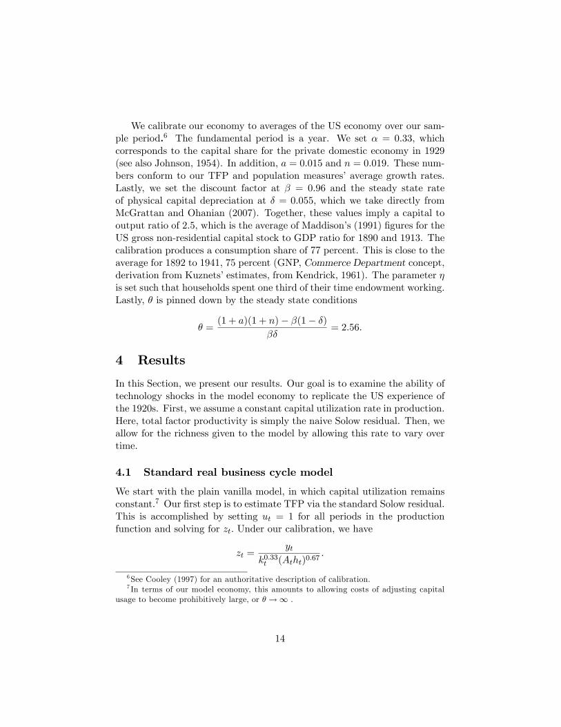
We calibrate our economy to averages of the US economy over our sam-ple period.6 The fundamental period is a year. We set � = 0:33; whichcorresponds to the capital share for the private domestic economy in 1929(see also Johnson, 1954). In addition, a = 0:015 and n = 0:019. These num-bers conform to our TFP and population measures�average growth rates.Lastly, we set the discount factor at � = 0:96 and the steady state rateof physical capital depreciation at � = 0:055; which we take directly fromMcGrattan and Ohanian (2007). Together, these values imply a capital tooutput ratio of 2:5, which is the average of Maddison�s (1991) �gures for theUS gross non-residential capital stock to GDP ratio for 1890 and 1913. Thecalibration produces a consumption share of 77 percent. This is close to theaverage for 1892 to 1941, 75 percent (GNP, Commerce Department concept,derivation from Kuznets�estimates, from Kendrick, 1961). The parameter �is set such that households spent one third of their time endowment working.Lastly, � is pinned down by the steady state conditions

� =(1 + a)(1 + n)� �(1� �)

��= 2:56:

4 Results

In this Section, we present our results. Our goal is to examine the ability oftechnology shocks in the model economy to replicate the US experience ofthe 1920s. First, we assume a constant capital utilization rate in production.Here, total factor productivity is simply the naive Solow residual. Then, weallow for the richness given to the model by allowing this rate to vary overtime.

4.1 Standard real business cycle model

We start with the plain vanilla model, in which capital utilization remainsconstant.7 Our �rst step is to estimate TFP via the standard Solow residual.This is accomplished by setting ut = 1 for all periods in the productionfunction and solving for zt: Under our calibration, we have

zt =yt

k0:33t (Atht)0:67:

6See Cooley (1997) for an authoritative description of calibration.7 In terms of our model economy, this amounts to allowing costs of adjusting capital

usage to become prohibitively large, or � !1 .

14

50

60

70

80

90

100

110

120

20 22 24 26 28 30 32 34 36 38 40

RBC USA

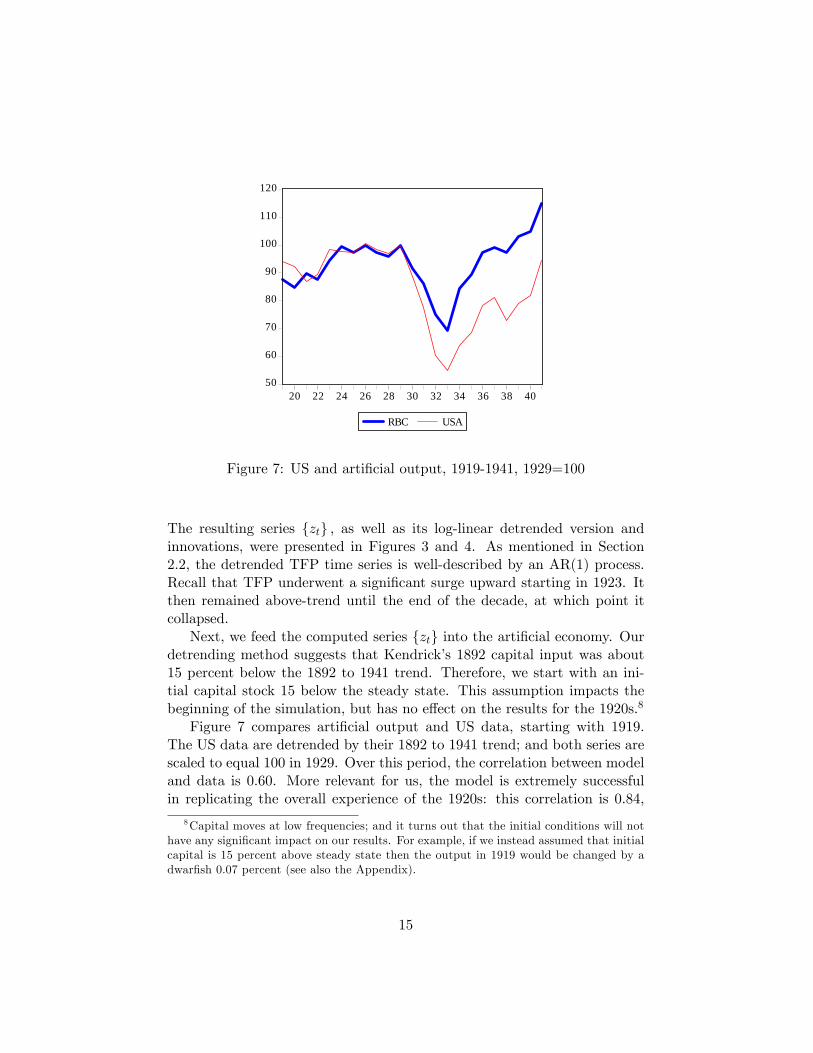
Figure 7: US and arti�cial output, 1919-1941, 1929=100

The resulting series fztg ; as well as its log-linear detrended version andinnovations, were presented in Figures 3 and 4. As mentioned in Section2.2, the detrended TFP time series is well-described by an AR(1) process.Recall that TFP underwent a signi�cant surge upward starting in 1923. Itthen remained above-trend until the end of the decade, at which point itcollapsed.

Next, we feed the computed series fztg into the arti�cial economy. Ourdetrending method suggests that Kendrick�s 1892 capital input was about15 percent below the 1892 to 1941 trend. Therefore, we start with an ini-tial capital stock 15 below the steady state. This assumption impacts thebeginning of the simulation, but has no e¤ect on the results for the 1920s.8

Figure 7 compares arti�cial output and US data, starting with 1919.The US data are detrended by their 1892 to 1941 trend; and both series arescaled to equal 100 in 1929. Over this period, the correlation between modeland data is 0.60. More relevant for us, the model is extremely successfulin replicating the overall experience of the 1920s: this correlation is 0.84,

8Capital moves at low frequencies; and it turns out that the initial conditions will nothave any signi�cant impact on our results. For example, if we instead assumed that initialcapital is 15 percent above steady state then the output in 1919 would be changed by adwar�sh 0.07 percent (see also the Appendix).

15

and for the period from 1922-1929 there is an almost perfect �t (0.92). Justlike in the data, the model�s 1920s peak is in 1926; and the 1929 value isindistinguishable from this peak. As for the three recessions, output risesin the model from 1920-21. Recalling that this recession has been largelyattributed to inept monetary policy (for example, Friedman and Schwartz,1963), this is not surprising. Model output also rises during the period of thenext, much milder, recession: from 1923-24. In both of these cases, however,model output falls in the year following the actual recession. TFP followedthe same pattern: rising during the recession years and falling after. Themodel, by attributing �uctuations only to changes in technology, thereforepredicts that both recessions come too late. The recession from 1926-27,is, however, well-captured by the model, with a simultaneous fall in TFPthat, as discussed above, re�ects the negative technology shock brought onby disruptions related to Ford�s closing of his factories to switch from ModelT to Model A. 9

4.2 Variable utilization

"E¤orts to measure the percentage utilization of the produc-tive capacity of real capital stocks are to be welcomed as addingto our information on explanatory variables. Unfortunately noreliable long-run measures of this variable are available eitherfor the business economy or for most of its individual divisions."[Kendrick, 1973, 26]

There is considerable evidence that utilization rates of capital vary sig-ni�cantly over the short and medium run. The subsequent issue of mis-measurement of TFP at business cycle frequencies goes back at least toSummers� (1986) critique of RBC theory. Unfortunately, we do not havedata for capital utilization over our sample period. Potential solutions tothis include the use of a proxy. For example, Burnside, Eichenbaum andRebelo (1995) employ electricity consumption and �nd that adjusted TFPis much less volatile than the naive Solow residual. Data on electricity pro-duction is in fact available for the 1920s. However, we are reluctant to useit because of the extraordinary structural changes in manufacturing�s use ofelectricity during the 1920s. It would be hard to distinguish between trendand cycle.

9The reader will also notice that the model�s fall in output starting in 1930 is not asdeep as that in the data. This evidence, that productivity cannot explain the weaknessof output, is reminiscent of that of Cole and Ohanian (1999), who �nd that technologyshocks cannot explain fully the depth of and weak recovery from the Great Depression.

16

Hence, we instead compute a series of model-consistent utilization rates.10

In particular, (1) determines the optimal utilization rate as a function ofboth output and the capital stock. We therefore compute11:

ut =

�0:33

ytkt

�1=2:56:

Figure 8 plots the detrended series futg. We see an unusually high, persistentand smooth rate of capital utilization during the 1920s: with 1929=100, theindex varies only from 94 to 101, and is on average quite high, especiallyover the later part of the decade. This is followed by a massive drop inutilization at the start of the Great Depression.12 The high rate in 1941very likely re�ects the e¤ects of the war in Europe on the United States.13

Next, a new series for total factor productivity is computed, accountingfor variable utilization, by

zt =yt

(utkt)0:33(Atht)0:67:

The resulting (log-linearly detrended) series is well-described by a �rst orderautoregressive process with � = 0:54.14 Utilization-adjusted TFP is plottedvis-a-vis the naive version in Figure 9 (normalized in 1929). Since utilizationof capital did not vary much during the 1920s, we expect the two series tobe highly correlated; and their correlation coe¢ cient is in fact 0.99. As istypical, adjusted TFP is less volatile, re�ecting factor hoarding.

Figure 10 displays arti�cial output, when shocked with utilization-adjustedTFP, and US data on per capita output between 1919 and 1941. Again, theUS data are detrended by their 1892 to 1941 trend and both series are scaledto equal 100 in 1929. The two series are again very similar. The year toyear correlation is about the same as the plain vanilla model�s: 0.61 versus0.60 for 1919-1941. Overall, the model again is able to replicate the eight

10See also Weder (2006).11When we apply the same procedure to post-war data, the resulting series replicates

well the Federal Reserve�s Industrial Production and Capacity Utilization Index. SeeAppendix.12As a benchmark for accuracy, Bresnahan and Ra¤ (1991) suggest that about twenty

percent of the aggregate capital stock lay fallow at the depth of the Depression in 1933. Ifwe interpret the values for 1929 being near full utilization, our constructed series matchesthis �gure.13For example, Roosevelt signed the Lend-Lease Act in early 1941, which committed

U.S. weapons to the Allied forces.14Utilization does not a¤ect long run TFP, as it does not follow a trend. Hence, the

growth rates of naive and adjusted TFP are indistinguishable

17

80

85

90

95

100

105

110

95 00 05 10 15 20 25 30 35 40

Capital utilization

Figure 8: Utilization rate of capital, 1892-1941, 1929=100

­.12

­.08

­.04

.00

.04

.08

70

80

90

100

110

95 00 05 10 15 20 25 30 35 40

Naive TFPAdjusted TFPAdjusted TFP shocks

Figure 9: Utilization adjusted TFP (detrended, 1929=100)

18

year boom followed by a massive four year drop in 1929. However, whenevaluated numerically, for the 1920-1929 stretch the arti�cial economy nowperforms worse: the correlation falls to 0.58 from 0.84. (Starting from 1922,however, there is a 73% correlation between model and data.) Since TFPagain falls only after each of the �rst two recessions, model output falls ayear too late in each case. In addition, the model now peaks too early �in1924; and this peak is about 4% higher than the value in 1929. Adjusting forutilization appears to take out some of the e¤ects of technological progressthat the naive accounting suggested for the 1920s.15

To better understand this result, Figure 11 displays the TFP input fromeach simulation. The two series correspond to the cycle component from Fig-ure 3 and the equivalent series constructed from utilization-adjusted TFP.While they appear to be almost identical, the movements of utilization-adjusted TFP are usually smaller, again re�ecting factor hoarding. Theonly exception is 1921 in which the adjusted TFP was larger. Again, otherfactors played a crucial role in this recession. Moreover, as can be seenfrom Figure 9, adjusted TFP is higher than the naive version during mostof the early 1920s. Together with the stronger propagation mechanism ofthe endogenous-utilization economy, this produces two e¤ects. First, thereis a larger response to TFP�s upswing in 1923 and 1924, resulting in outputthat is too high relative to data. Second, once either model is away from its(stable) steady state, it endogenously reverts back to it. This e¤ect is alsostronger in the variable utilization model, so output declines relative to theplain vanilla model, and to the US data. The second e¤ect dominates later,since shocks to TFP are relatively small after 1924. In summary, the pre-dictions for the 1920s of the utilization-corrected model are less successfulthan those of the standard RBC model.

5 Concluding remarks

This paper has examined the origins of the Roaring Twenties in the UnitedStates. In particular, we applied a version of the real business cycle modelto test the hypothesis that an exceptional pace of productivity growth wasthe driving factor behind eight extraordinary years of economic boom.

Our motivation comes from abundant evidence of signi�cant technolog-ical progress during this period. In particular, process innovations and the

15However, the model�s performance is about the same as the standard RBC model�sfor the 1930s. This supports Ohanian�s (2001) suggestion that accounting for utilizationshould not much a¤ect the RBC model�s predictions for the Great Depression.

19

50

60

70

80

90

100

110

120

20 22 24 26 28 30 32 34 36 38 40

RBC USA

Figure 10: Arti�cial economy (variable capital utilization, 1929=100)

­.20

­.15

­.10

­.05

.00

.05

.10

.15

20 22 24 26 28 30 32 34 36 38 40

TFP TFP (adjusted)

Figure 11: TFP (percentage) deviations from trend

20

widespread adoption of electricity in manufacturing and in particular thefrictional horsepower electric motor led to economy-wide increases in pro-ductivity. Therefore, we have included only technology shocks here. In fact,this paper is the �rst that numerically evaluates the general equilibrium ef-fects of the technological change on the US economy during the 1920s. Usinga plain vanilla RBC model, our estimated TFP shocks lead to arti�cial out-put series that are highly correlated with the data, especially over the period1922-1929. Since these years are generally considered the de�ning ones forthe 1920s, we take it from our analysis, that extraordinary technologicalchange was the main force behind the Roaring Twenties. The model alsopredicts well the 1926-27 recession. However, when we allow for variablecapital utilization, the model is considerably less successful at replicatingboth the general nature of the decade, and its ups and downs.

In the future we may extend this analysis in several di¤erent directions.More information may be gleaned from a model in which technical changeis allowed to be investment-speci�c. In addition, Olney (1991) attributesmuch of the robustness of growth during the 1920s to the expansion of theavailability of credit. A model that incorporates this feature of the economywould shed more light on this unique episode in U.S. economic history.

References

[1] Allen, Frederick Lewis (1931): Only Yesterday, Harper & Row, NewYork.

[2] Atack, Jeremy and Peter Passell (1994): A New Economic View ofAmerican History, W.W. Norton New York.

[3] Berry, Thomas S. (1988): Production and Population Since 1789: Re-vised GNP Series in Constant Dollars, The Bostwick Press, Richmond.

[4] Bordo, Michael D., Christopher J. Erceg and Charles N. Evans (2000):"Money, Sticky Wages and the Great Depression", American EconomicReview 90, 1447-1463.

[5] Bresnahan, Timothy F. and Daniel M. Ra¤(1991): "Intra-industry Het-erogeneity and the Great Depression: The American Motor VehiclesIndustry, 1929�1935", Journal of Economic History 51, 317�331.

[6] Burnside, Craig, Martin Eichenbaum and Sergio Rebelo (1995): "Cap-ital Utilization and Returns to Scale", NBER Macroeconomics Annual10, 67-110.

21

[7] Cole, Hal L. and Lee E. Ohanian (1999): "The Great Depression in theUnited States from a Neoclassical Perspective", Federal Reserve Bankof Minneapolis Quarterly Review 23, 2-24.

[8] Cole, Hal L. and Lee E. Ohanian (2004): "New Deal Policies and thePersistence of the Great Depression: A General Equilibrium Analysis",Journal of Political Economy 112, 779-816.

[9] Cooley, Thomas F. (1997): "Calibrated Models ", Oxford Review ofEconomic Policy 13, 55-69.

[10] Devine, Warren D., Jr. (1983): "From Shafts to Wires: Historical Per-spectives on Electri�cation", The Journal of Economic History 43, 347-372.

[11] Evans, Charles L. (1992): "Productivity Shocks and Real Business Cy-cles", Journal of Monetary Economics 29, 191-208

[12] Field, Alexander (2003): "The Most Technologically ProgressiveDecade of the Century", American Economic Review 93, 1399-1414.

[13] Field, Alexander (2006): "Technological Change and U.S. ProductivityGrowth in the Interwar Years", The Journal of Economic History, 66,203-236.

[14] Field, Alexander (2008): "US Economic Growth in the Gilded Age",Journal of Macroeconomics (forthcoming).

[15] Freidman, Milton and Anna Jacobson Schwartz (1963): A MonetaryHistory of the United States, 1867-1960, Princeton University Press,Princeton.

[16] Greenwood, Jeremy, Zvi Hercowitz and Gregory Hu¤man (1988): "In-vestment, Capacity Utilization, and the Real Business Cycle", Ameri-can Economic Review 78, 402-417.

[17] Harrison, Sharon G. and Mark Weder (2006): "Did Sunspot ForcesCause the Great Depression?", Journal of Monetary Economics 53,1327-1339.

[18] Harrison, Sharon G. and Mark Weder (2008): �Technology, Credit andCon�dence During the Roaring Twenties�, Barnard College and Uni-versity of Adelaide, mimeographed.

22

[19] Johnson, G. (1954): "The Functional Distribution of Income in theUnited States 1850-1952", Review of Economics and Statistics 36, 175-182.

[20] Kendrick, John W. (1961): Productivity Trends in the United States,Princeton University Press, Princeton.

[21] Kendrick, John W. (1973): Postwar Productivity Trends in the UnitedStates 1948-1969, Princeton University Press, Princeton.

[22] Kyvig, David E. (2002): Daily Life in the United States, 1920-1939:Decades of Promise and Pain, Greenwood Press.

[23] McGrattan, Ellen R. and Lee E. Ohanian (2007): "Does NeoclassicalTheory Account for the E¤ects of Big Fiscal Shocks? Evidence fromWorld War II", Sta¤Report 315, Federal Reserve Bank of Minneapolis.

[24] McGrattan, Ellen R. (2006): "Real Business Cycles", in: The New Pal-grave Dictionary of Economics, 2nd Ed (forthcoming).

[25] Maddison, Angus (1991): Dynamic Forces in Capitalist Development,Oxford University Press, Oxford.

[26] Ohanian. Lee E. (2001): "Why Did Productivity Fall So Much duringthe Great Depression?", American Economic Review 91, 34-38.

[27] Olney, Martha (1991): Buy Now, Pay Later: Advertising, Credit andConsumer Durables in the 1920s, The University of North CarolinaPress.

[28] Oshima, Harry T. (1984): "The Growth of U.S. Factor Productivity:The Signi�cance of New Technologies in the Early Decades of the Twen-tieth Century", The Journal of Economic History 44, 161-70.

[29] Report of the Committee on Recent Economic Changes of the Pres-ident�s Conference on Unemployment (1929), in Recent EconomicChanges in the United States, Volumes 1 and 2

[30] Romer, Christina D. (1989): "The Prewar Business Cycle Reconsidered:New Estimates of Gross National Product, 1869-1908", The Journal ofPolitical Economy 97, 1-37.

[31] Schurr, Samuel H. and Bruce C. Netschert (1960): Energy in the Amer-ican Economy, 1850-1975, John Hopkins Press, Baltimore.

23

[32] Smiley, Gene (2008): "US Economy in the 1920s".EH.Net Encyclopedia, edited by Robert Whaples,http://eh.net/encyclopedia/article/Smiley.1920s.�nal

[33] Summers, Lawrence H. (1986): "Some Skeptical Observations on RealBusiness Cycle Theory", Quarterly Review Federal Reserve Bank ofMinneapolis, 23-27.

[34] Temin, Peter (2008): "Real Business Cycle Views of the Great Depres-sion and Recent Events: A Review of Timothy J. Kehoe and EdwardC. Prescott�s Great Depressions of the Twentieth Century", Journal ofEconomic Literature 46, 669�84.

[35] Weder, Mark (2006): "The Role of Preference Shocks and Capital Uti-lization in the Great Depression", International Economic Review 47,1247-1268.

[36] Weir, David (1986): "The Reliability of Historical Macroeconomic Datafor Comparing Cyclical Stability, Journal of Economic History 46, 353-365.

6 Appendix

This Appendix presents robustness checks of our reported results. First, weshow that our data representation is not overly dependent on the detrendingmethod. Let us follow Cole and Ohanian (1999) and trend-adjust by dividingoutput by its 20th century long-run trend growth rate �1.9 percent relativeto the reference date. Figure 12 illustrates. Except for the brief 1906-07boom, the US economy did not spend much time as aloft as in 1920s. Overall,the higher trend does not change the punch-line of our paper. We arereluctant to use the "1.9 percent de�ator" since TFP grew at a much smallerrate during the prewar era: the 1892 to 1941 grow rate was about 1.5 percent.Perhaps it is sensible to assume that there was a structural break after thewar, in any case, we do not elaborate on this break issue here. Hence, wede�ate by the prewar rate in the paper. We also note that our cyclicaloutput time series is very similar to Berry�s (1988).

Our other robustness check involves our decision to begin our simulationsin 1892 with an initial capital stock 15% below trend. To show the smalle¤ect of this� resulting from the low frequency movements of the capitalstock �we alternatively begin the simulation in 1919 with an initial capitalstock that is ten percent below the model steady state. The ten percent

24

50

60

70

80

90

100

110

95 00 05 10 15 20 25 30 35 40

US output

1929=100

Figure 12: Detrended per capita output

re�ect the resulting value after detrending the series on capital. Figure 13shows that this has a negligible e¤ect.

Figure 14 shows that our capital utilization series is very similar to theFederal Reserve Bank�s measure. The �t is not perfect but in the absence ofany data for the 1920s, we have used our best estimate. The correlation is0.72 overall, and 0.92 for the �rst twenty years. The two series diverge themost in the second half of the 1990s. This likely re�ects IT-related structuralchanges �i.e. a break in trend �in the US economy (source of data: BEA).

Lastly, using the sample 1919-1941, we test if technology evolves exoge-nously. The results for an Evans (1992) like test were

lnz0t+1 = 2:53(2:33)

+ 0:44(1:86)

lnz0t � 0:003(0:60)

�mt � 0:003(0:23)

it � 0:00001(0:58)

�Gt

where the numbers in parenthesis are absolute t statistics. Here z0 denotes(detrended) TFP, �mt stands for the change in M2, i is the three monthTreasury Bill and �Gt is the change in (real) government purchases. Allthree additional variables were found to be statistically insigni�cant. Uti-lization adjusted TFP yields similar results.

25

60

70

80

90

100

110

120

20 22 24 26 28 30 32 34 36 38 40

Simulation starting 1919Simulation starting 1892

Figure 13: Simulation with di¤erent intial conditions.

64

68

72

76

80

84

88

92

1960 1965 1970 1975 1980 1985 1990 1995 2000 2005

Utilization rate from focIndustrial Production and Capacity Utilization (Manufacturing, SIC)

Figure 14: Capital utilization rates

26

www.st-and.ac.uk/cdma

ABOUT THE CDMA

The Centre for Dynamic Macroeconomic Analysis was established by a direct grant from theUniversity of St Andrews in 2003. The Centre funds PhD students and facilitates a programme ofresearch centred on macroeconomic theory and policy. The Centre has research interests in areas such as:characterising the key stylised facts of the business cycle; constructing theoretical models that can matchthese business cycles; using theoretical models to understand the normative and positive aspects of themacroeconomic policymakers' stabilisation problem, in both open and closed economies; understandingthe conduct of monetary/macroeconomic policy in the UK and other countries; analyzing the impact ofglobalization and policy reform on the macroeconomy; and analyzing the impact of financial factors onthe long-run growth of the UK economy, from both an historical and a theoretical perspective. TheCentre also has interests in developing numerical techniques for analyzing dynamic stochastic generalequilibrium models. Its affiliated members are Faculty members at St Andrews and elsewhere withinterests in the broad area of dynamic macroeconomics. Its international Advisory Board comprises agroup of leading macroeconomists and, ex officio, the University's Principal.

Affiliated Members of the School

Dr Fabio Aricò.Dr Arnab Bhattacharjee.Dr Tatiana Damjanovic.Dr Vladislav Damjanovic.Prof George Evans.Dr Gonzalo Forgue-Puccio.Dr Laurence Lasselle.Dr Peter Macmillan.Prof Rod McCrorie.Prof Kaushik Mitra.Prof Charles Nolan (Director).Dr Geetha Selvaretnam.Dr Ozge Senay.Dr Gary Shea.Prof Alan Sutherland.Dr Kannika Thampanishvong.Dr Christoph Thoenissen.Dr Alex Trew.

Senior Research Fellow

Prof Andrew Hughes Hallett, Professor of Economics,Vanderbilt University.

Research Affiliates

Prof Keith Blackburn, Manchester University.Prof David Cobham, Heriot-Watt University.Dr Luisa Corrado, Università degli Studi di Roma.Prof Huw Dixon, Cardiff University.Dr Anthony Garratt, Birkbeck College London.Dr Sugata Ghosh, Brunel University.Dr Aditya Goenka, Essex University.Prof Campbell Leith, Glasgow University.Prof Paul Levine, University of Surrey.Dr Richard Mash, New College, Oxford.Prof Patrick Minford, Cardiff Business School.Dr Gulcin Ozkan, York University.Prof Joe Pearlman, London Metropolitan University.

Prof Neil Rankin, Warwick University.Prof Lucio Sarno, Warwick University.Prof Eric Schaling, South African Reserve Bank and

Tilburg University.Prof Peter N. Smith, York University.Dr Frank Smets, European Central Bank.Prof Robert Sollis, Newcastle University.Prof Peter Tinsley, Birkbeck College, London.Dr Mark Weder, University of Adelaide.

Research Associates

Mr Nikola Bokan.Mr Farid Boumediene.Mr Johannes Geissler.Mr Michal Horvath.Ms Elisa Newby.Mr Ansgar Rannenberg.Mr Qi Sun.

Advisory Board

Prof Sumru Altug, Koç University.Prof V V Chari, Minnesota University.Prof John Driffill, Birkbeck College London.Dr Sean Holly, Director of the Department of Applied

Economics, Cambridge University.Prof Seppo Honkapohja, Bank of Finland and

Cambridge University.Dr Brian Lang, Principal of St Andrews University.Prof Anton Muscatelli, Heriot-Watt University.Prof Charles Nolan, St Andrews University.Prof Peter Sinclair, Birmingham University and Bank of

England.Prof Stephen J Turnovsky, Washington University.Dr Martin Weale, CBE, Director of the National

Institute of Economic and Social Research.Prof Michael Wickens, York University.Prof Simon Wren-Lewis, Oxford University.

www.st-and.ac.uk/cdmaRECENT WORKING PAPERS FROM THE

CENTRE FOR DYNAMIC MACROECONOMIC ANALYSIS

Number Title Author(s)

CDMA07/10 Optimal Sovereign Debt Write-downs Sayantan Ghosal (Warwick) andKannika Thampanishvong (StAndrews)

CDMA07/11 Bargaining, Moral Hazard and SovereignDebt Crisis

Syantan Ghosal (Warwick) andKannika Thampanishvong (StAndrews)

CDMA07/12 Efficiency, Depth and Growth:Quantitative Implications of Financeand Growth Theory

Alex Trew (St Andrews)

CDMA07/13 Macroeconomic Conditions andBusiness Exit: Determinants of Failuresand Acquisitions of UK Firms

Arnab Bhattacharjee (St Andrews),Chris Higson (London BusinessSchool), Sean Holly (Cambridge),Paul Kattuman (Cambridge).

CDMA07/14 Regulation of Reserves and InterestRates in a Model of Bank Runs

Geethanjali Selvaretnam (StAndrews).

CDMA07/15 Interest Rate Rules and Welfare in OpenEconomies

Ozge Senay (St Andrews).

CDMA07/16 Arbitrage and Simple Financial MarketEfficiency during the South Sea Bubble:A Comparative Study of the RoyalAfrican and South Sea CompaniesSubscription Share Issues

Gary S. Shea (St Andrews).

CDMA07/17 Anticipated Fiscal Policy and AdaptiveLearning

George Evans (Oregon and StAndrews), Seppo Honkapohja(Cambridge) and Kaushik Mitra (StAndrews)

CDMA07/18 The Millennium Development Goalsand Sovereign Debt Write-downs

Sayantan Ghosal (Warwick),Kannika Thampanishvong (StAndrews)

CDMA07/19 Robust Learning Stability withOperational Monetary Policy Rules

George Evans (Oregon and StAndrews), Seppo Honkapohja(Cambridge)

CDMA07/20 Can macroeconomic variables explainlong term stock market movements? Acomparison of the US and Japan

Andreas Humpe (St Andrews) andPeter Macmillan (St Andrews)

www.st-and.ac.uk/cdmaCDMA07/21 Unconditionally Optimal Monetary

PolicyTatiana Damjanovic (St Andrews),Vladislav Damjanovic (St Andrews)and Charles Nolan (St Andrews)

CDMA07/22 Estimating DSGE Models under PartialInformation

Paul Levine (Surrey), JosephPearlman (London Metropolitan) andGeorge Perendia (LondonMetropolitan)

CDMA08/01 Simple Monetary-Fiscal Targeting Rules Michal Horvath (St Andrews)

CDMA08/02 Expectations, Learning and MonetaryPolicy: An Overview of Recent Research

George Evans (Oregon and StAndrews), Seppo Honkapohja (Bankof Finland and Cambridge)

CDMA08/03 Exchange rate dynamics, asset marketstructure and the role of the tradeelasticity

Christoph Thoenissen (St Andrews)

CDMA08/04 Linear-Quadratic Approximation toUnconditionally Optimal Policy: TheDistorted Steady-State

Tatiana Damjanovic (St Andrews),Vladislav Damjanovic (St Andrews)and Charles Nolan (St Andrews)

CDMA08/05 Does Government Spending OptimallyCrowd in Private Consumption?

Michal Horvath (St Andrews)

CDMA08/06 Long-Term Growth and Short-TermVolatility: The Labour Market Nexus

Barbara Annicchiarico (Rome), LuisaCorrado (Cambridge and Rome) andAlessandra Pelloni (Rome)

CDMA08/07 Seignioprage-maximizing inflation Tatiana Damjanovic (St Andrews)and Charles Nolan (St Andrews)

CDMA08/08 Productivity, Preferences and UIPdeviations in an Open EconomyBusiness Cycle Model

Arnab Bhattacharjee (St Andrews),Jagjit S. Chadha (Canterbury) and QiSun (St Andrews)

CDMA08/09 Infrastructure Finance and IndustrialTakeoff in the United Kingdom

Alex Trew (St Andrews)

..

For information or copies of working papers in this series, or to subscribe to email notification, contact:

Johannes GeisslerCastlecliffe, School of Economics and FinanceUniversity of St AndrewsFife, UK, KY16 9ALEmail: jg374@at-andrews.ac.uk; Phone: +44 (0)1334 462445; Fax: +44 (0)1334 462444.