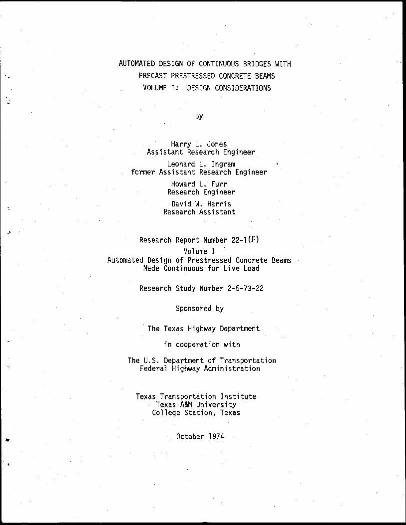
.t

1. Report No. 2. Government Accession No.

4. Title and Subtitle

AUTOMATED DESIGN OF CONTINUOUS BRIDGES WITH PRECAST PRESTRESSED CONCRETE BEAMS--VOLUME I: DESIGN CON~ SIDERATIONS 7, Authorl s) Harry L. Jones Leonard L. Ingram

Howard L. Furr David W. Harris

9, Performing Orgoni zotion Name and Address

Texas Transportation Institute Texas A&M University College Station, Texas 77843

TECHNICAL REPORT STANDARD TITLE PACf

3. Recipient's Catalog No.

5. Report Date

October 1974 6. Performing Organization Code

8. Performing Organization Report No.

Research Report 22-lF

10. Work Unit No.

11. Contract or Grant No.

1-;-;;--;-~--:---:--:---~---:--:-:-:--------------------J 13. Type of Report and Period Covered 12. Sponsoring Agency Name and Address

Texas Highway Department 11th and Brazos Austin, Texas 78701

Final - September 1972 October 1974

14. Sponsoring Agency Code

1 S. Supplementary Notes Research performed in cooperation with DOT, FHWA

~ Research Study Title: "Automated Design of Prestressed Concrete Beams Made Con-tinuous for Live Load"

16. Abstract

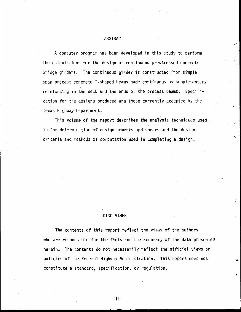
A computer program has been developed in this study to perform the calculations for the design of continuous prestressed concrete bridge girders. The continuous girder is constructed from simple span precast concrete.I-shaped beams made con­tinuous by supplementary·reinforcing in the deck and the ends of the precast beams. Specification for the designs produced are those currently accepted by the Texas Highway Department.

This volume of the report describes the analysis techniques used in the deter­mination of design moments and shears and the design criteria and methods of com­putation used in completing a design.

17. Key Words , Cont1nuous Bridges, Precast Prestressed Concrete Beams, Computer Program, Design

18. Distribution Statement

19. Security Clouif. (of this report)

Unclassified

20. Security Claaaif. (of this page)

Unclassified

Form DOT F 1700.7 CB·69l

21. No. of Pages 22. Price

58

!

r .....

..

AUTOMATED DESIGN OF CONTINUOUS BRIDGES WITH PRECAST PRESTRESSED CONCRETE BEAMS

VOLUME I: DESIGN CONSIDERATIONS

by

Harry L. Jones Assistant Research Engineer

Leonard L. Ingram former Assistant Research Engineer

Howard L. Furr Research Engineer David W. Harris

Research Assistant

Research Report Number 22-l(f) Volume I

Automated Design of Prestressed Concrete Beams Made Continuous for Live Load

Research Study Number 2-5-73-22

Sponsored by

The Texas Highway Department

in cooperation with

The U.S. Department of Transportation Federal Highway Administration

Texas Transportation Institute Texas A&M University

College Station, Texas

October 1974

ABSTRACT

A computer program has been developed in this study to perform

the calculations for the design of continuous prestressed concrete

bridge girders. The continuous girder is constructed from simple

span precast concrete !-shaped beams made continuous by supplementary

reinforcing in the deck and the ends of the precast beams. Specifi~

cation for the designs produced are those currently accepted by the

Texas Highway Department.

This volume of the report describes the analysis techniques used

in the determination of design moments and shears and the design

criteria and methods of computation used in completing a design.

DISCLAIMER

The contents of this report reflect the views of the authors

who are responsible for the facts and the accuracy of the data presented

herein. The contents do not necessarily reflect the official views or

policies of the Federal Highway Administration. This report does not

constitute a standard, specification, or regulation.

ii

:

...

SUMMARY

This report describes the analysis techniques and design calcula­

tions used in a computer program developed for the design of continuous

prestressed concrete bridge girders. The continuous girder is con­

structed from simple span precast prestressed concrete !-shaped beams

made continuous by supplemental reinforcing in the deck and the ends of

the beam. The program is limited to continuous girders in which precast

.beams in all spans are of identical shape. The program considers live

loads produced by standard AASHTO trucks and lane loadings, by an 11 axle

train 11 of up to 15 wheels of arbitrary weight and spacing and by a uni­

form distributed load on the continuous beam. Dead load due to beam

weight, diaphrams and slab weight are also included. Provisions are

made to treat cases where a portion of the deck over interior supports

is cast first to establish continuity and the remaining deck weight is

carried by the continuous beam.

The program computes for each span of the girder the number of pre­

stressing strands and their placement, the area of conventional rein­

forcing required in the deck to resist negative moment, the area of rein­

forcing required at interior supports to resist positive moment and the

spacing of stirrups.

iii

RECOMMENDATION FOR IMPLEMENTATION

A computer program was developed in this study to carry out the

necessary calculations for the design of continuous bridge girders

constructed from simple span precast prestressed concrete !-shaped

beams.

This program is being used by the Texas Highway Department, and

its continued use is recommended.

iv

ABSTRACT •

SUMMARY ..

TABLE OF CONTENTS Page

ii

. • iii

RECOMMENDATION FOR IMPLEMENTATION.

LIST OF FIGURES.

. . . . i v

vi

LIST OF TABLES . . . vii

I. INTRODUCTION . 1

II. LIVE LOAD AND DEAD LOAD SHEAR AND MOMENT COMPUTATIONS. 3

2.1 Influence Lines for Continuous Beams. . . . . . . . . 3 2.2 Maximum and Minimum Values for Moment and Shear-

Moving Loads. . . . . . • . . . . • • . . . . . • 9 2.3 Maximum and Minimum Values for Moment and Shear-

Lane and Uniformly Distributed Loads. . . . . 11 2.4 Moments and Shears Produced by Dead Loads . 14

III. CREEP AND SHRINKAGE RESTRAINT FORCE COMPUTATIONS . . . . . 15

3.1 Computation of Unsealed Restraint Moments ...... 17 3.2 Computation of Scale Factors for Restraint

Moments . . 22

IV. DESIGN CRITERIA. • . . . 30

4.1 Predesign Decisions • 30 4.2 Beam Design Loads . . . . . . . . . . . . . . . 31 4.3 Criteria for Strand Pattern Selection . . . . . . 32 4.4 Computation of Positive Ultimate Moment Capacity. 41 4.5 Computation of Negative Moment Deck Reinforcement 51 4.6 Computation of Positive Moment Reinforcement at

Supports. . . . . . . . . . . . . . . . • . 55 4.7 Computation of Shear Reinforcing 55

REFERENCES . . . . . . . . . . • . . . . 58

v

No.

1

2

3

4

5

6

7

8

9

10

11

12

13

14

LIST OF FIGURES

Title

Continuous Beam with N Spans

Influence Lines for Moment and Shear .

Start and Terminal Positions for Axle Train at Extreme Point 1. . . . . . . . . . . . . . . .

Starting and Terminal Configurations for HS-Truck.

Creep Restraint Moments ....

Shrinkage Restraint Moments ..

Fixed End Moments for Dead Load Creep.

Fixed End Moments for Prestress Creep.

Fixed End Moments for Shrinkage ..

Shrinkage Strain Correction Factor ..

Shrinkage Humidity Correction Factor ..

Variables Defining Strand Pattern .•

Stress and Strain Profiles at Ultimate for Positive Moment . . . . . . . . . . . . . . . . . . . . .

Stress-Strain Curves for Prestressing Strands ...

15 Comparison of Moment Capacities for Neutral Axis in

Page

4

10

12

13

16

18

19

20

21

26

28

35

47

48

Slab . . . . . . . . . . . . . . . . . . . . . . 50

16

17

Stress and Strain Profiles at Ultimate for Negative Moment at Interior Tenth Points ..•........

Stress and Strain Profile at Ultimate for Negative Moment at End of Beam. . . . . . . . • . . . . . .

vi

52

53

\.

.-

--

LIST OF TABLES

No. Title Page

1 Strength and Moduli Values from Reference (I). . . 24

2 Expressions for Shrinkage Strain and Unit Creep Strain for 3 in. x 3 in. x 16 in. Prisms Stored Under Laboratory Conditions. . . 24

3

4

5

6

Location of Hold Down Points .

Stress Checks for Design ...

Verbal Description of Constraints.

Standard Longitudinal T~mperature and Distribu-tion Reinforcing ............... .

vii

. 33

33

. . 42

46

·-

•

J

I. INTRODUCTION

This report provides a general description of the design considera­

tions incorporated in a computer program for the automated design of

continuous bridges, constructed with precast, prestressed concrete beams.

This type of bridge differs from conventional simple span prestressed

concrete beam and cast-in-place deck construction in that the deck slab

is continuous over interior supports and is reinforced to withstand

negative moments arising from continuity. The construction sequence for

such a structure consists of placement of the beams on bent caps and

pouring of a portion of the deck over each interior support to establish

continuity. After the initial continuity pours have gained sufficient

strength, the remaining segments of deck are cast. A common variation on

this construction sequence is the casting of the entire deck at one time,

without the initial continuity pours. The first construction sequence

subjects the simple span beams to the dead load force of the initial deck

segment placed for continuity, while the remainder of the dead load of

the slab and all subsequent 1 ive loads are carried by the continuous beam.

·This mode of construction is said to be partially continuous for dead load.

In the latter construction sequence, all dead load produced by the deck is

carried by the simple beams, while subsequent live loads are carried by

the continuous beam. This construction sequence is said to be continuous

for live load only.

With either method, some economy in design is obtained through the

reduction of the maximum positive moments that a beam must sustain. The

design of this type of bridge beam requires certain additional considera­

tions which do not arise in the design of simple span prestressed concrete

1

highway beams. The computation of live load moments and shears involves

the analysis of a statically indeterminate structure. In addition, if

the bridge is partially continuous for dead load, the forces produced by

the casting of the remainder of the deck must be obtained from an indeter­

minate structural analysis. Concrete bridge structures are subject to

time dependent deformations produced by creep of the deck and beam concrete . and by differential shrinkage between the deck and beams. In continuous

structures, these deformations cannot occur freely due to the restraint

of continuity. As a result, additional moments and shears are produced in

the beam which must be considered during design. Negative moments are

produced in the continuous beam by live loads and by a portion of the dead

load of the deck in the case of beams partially continuous for dead load.

The negative moments are resisted by conventional reinforcing bars, whose

required area must be determined at those sections which resist negative

moment.

This mode of construction depends on adequate continuity connections

at interior supports. References 4 and 8 devote considerable attention

to the details of such a connection and the reader is referred to these

studies for additional information.

The remainder of this report describes the design calculations and

analysis methodology incorporated in the computer program. Sections II

and III are devoted to the development of analysis techniques to determine

the forces which the bridge beam must sustain, while Section IV describes

the design criteria on which the program is based. The details of program

operation, and specific instructions for its use are contained in Vol. II

of this report.

2

•

.:

J

II. LIVE LOAD AND DEAD LOAD SHEAR AND MOMENT COMPUTATIONS

The most expedient means of determining the maximum and minimum

moments and largest (in absolute value) shear force produced at a point

in a continuous beam by moving or variable loads is through the use of

influence lines. The method found to be the most efficient computa­

tionally for the requirements of this work is construction of influence

lines for the reactions of the beam. The influence lines for both shear

and moment at a specified point can then be constructed directly through

the application of statics and these in turn are utilized for the calcu­

lation of live load and dead load design moments and shears.

2.1 Influence Lines for Continuous Beams

Consider the continuous prismatic beam of N spans with (N+l) reaction

forces, shown in Fig. 1. The computation of reaction forces R1 , ... , RN+l

produced by the unit load at position Z can be accomplished through the

application of Castigliano•s Second Theorem. That is,

i=l, ... , (N-1) (1)

In Equation (1), Ri is the ith support reaction, and the expression applies

to only (N-1) of the reactions which are chosen as redundant. Let

i

1 i = I: Li j=l

3

1 =0 0

(2)

N

)(

4

z ..J

I z ..J

C\1 I z

..J

I() ..J

C\1 ..J

..J

en z ~

I en z a: z

J: 1-3=

... ~ <( w m en ::::> 0

"'" ::::>

a: z 1-z 0 u _:

w a:: I() ::::> a: ~

u..

C\1 a:

:

J

·.

l(x-a)n (x-a>" =

0

; x.:_a

; x<a

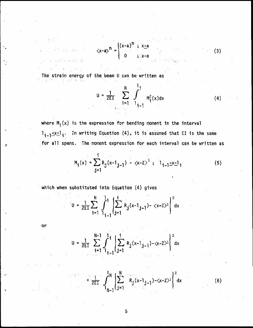
The strain energy of the beam U can be written as

LN Jli

U - 1 - 2EI M~(x)dx

i=l li-1

where Mi(x) is the expression for bending moment in the interval

(3)

(4)

1. 1<x<1 .. In writing Equation (4), it is assumed that EI is the same 1- -- 1

for all spans. The moment expression for each interval can be written as

i . I: 1 M. (x) = R. (x-1 . 1) - (x-Z) ; 1 J J-

j=1 1. 1 <X<l. ,_-- 1

which when substituted into Equation (4) gives

or

. N 1 . I i . 2

· U = 2 ~ 1 ~ j1 ~ Rj (x-1 j-l )- (x-Z)1 dx

1=1 li-1 J=l

- 1 U - 2EI

5

(5)

(6)

Equation (6) contains reactions R1 through RN. Since the structure is

indeterminate to the (N-1) degree, only (N-1) reaction forces may be

treated as independent variables in Equation (6). Applying statics

through the summation of moments about support (N+l) yields the following

expression for RN in terms of the remaining {N-1) independent reactions.

(7}

Hence, Equation (6) becomes

N-1 ·r: j=l

(8)

The application of Equation (1) to Equation (8) yields (N-1) linear

equations in the (N-1) redundant reactions R1, ..• , RN-l" This system of

equations can be conveniently written in matrix notation as

[A][R] = [li] (9)

6

I

·.

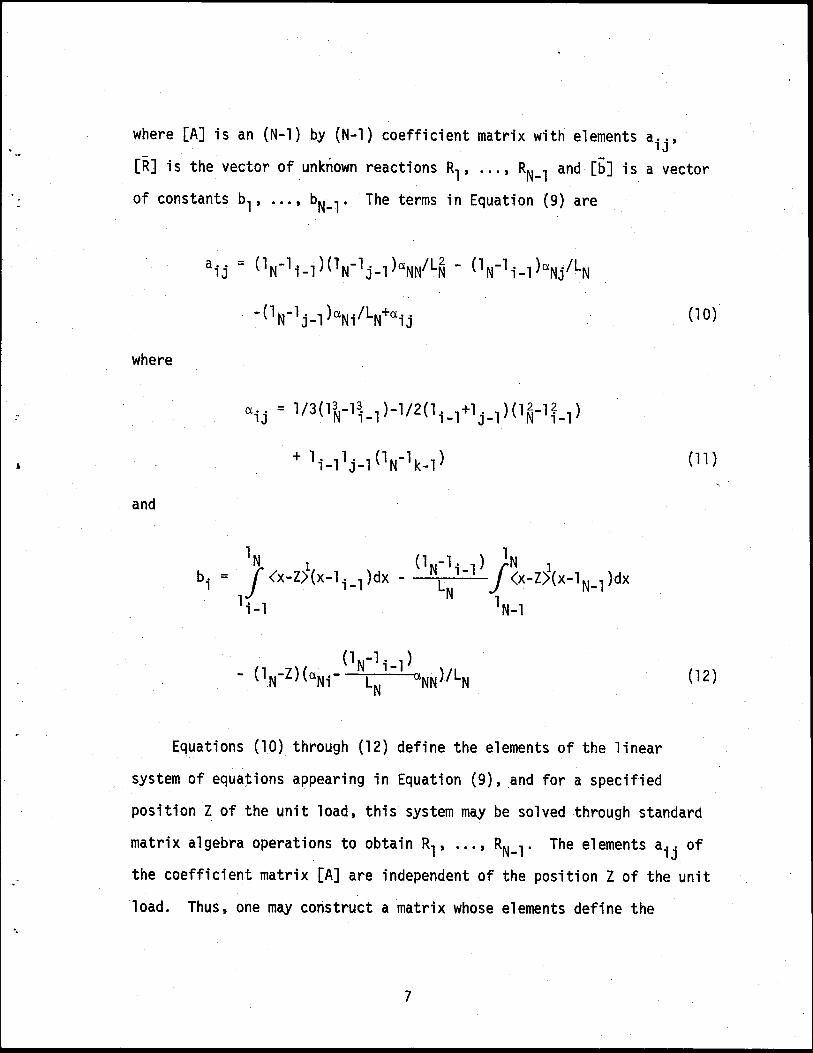
where [A] is an (N-1) by {N-1) coefficient matrix with elements aij'

[R] is the vector of unknown reactions R1 , ... , RN-l and [b] is a vector

of constants b1, •.. , bN-l' The terms in Equation (9) are

- { l N·.- l • 1 ) a.N. /LN+a. .. J- 1 lJ {lO)

where

(11)

and

( 12)

Equations (10) through (12) define the elements of the linear

system of equations appearing in Equation (9), and for a specified

position Z of the unit load, this system may be solved through standard

matrix algebra operations to obtain R1, .•• , RN-l' The elements aij of

the coefficient matrix [A] are independent of the position Z of the unit

load. Thus, one may construct a matrix whose elements define the

7

reaction forces for a number of different unit load positions (e.g.,

Z=l ft, Z=2 ft, ... , Z=lN ft) by writing

[A][R] = [B]

where

and

The term bi in Equation (15) is obtained from Equation (12), with Z

being the jth value of Z (unit load j ft from the left support).

( 13)

(14)

( 15)

Equation (13) can be solved for the matrix of support reactions [B] quite

effeciently by a standard computer routine. If the solution to Equation (13)

is stored in the matrix [B],' the element in the ith row and jth column of

[B] is the value of Ri when the unit load is j ft from the left support.

The values of shear and moment at a point y ft from the left end of

the beam and with the unit load Z ft from the left end of the beam follow

from statics to give

N+l

V = L: R;(Y-1;_1>0-l.O

i=l

8

( 16)

'

.·

.•

·-

N

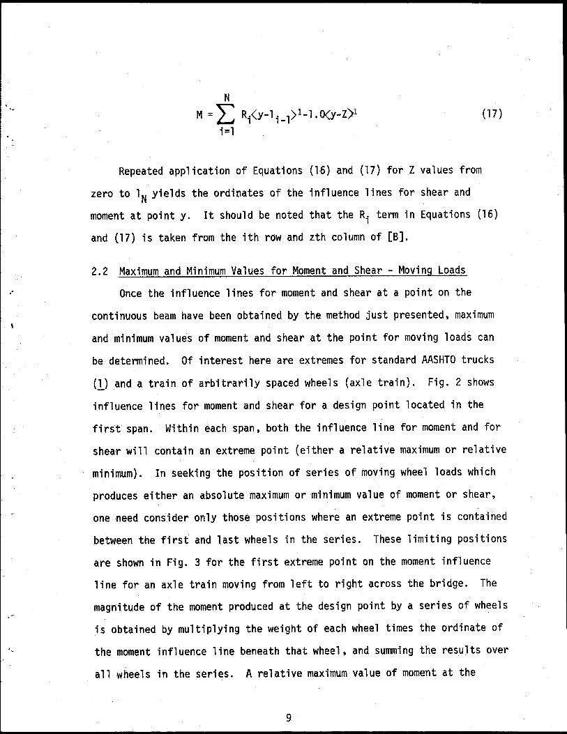
M =I: Ri(y-1 i _1)1-1. O(y-Z)l i=l

(17)

Repeated application of Equations (16) and (17) for Z values from

zero to lN yields the ordinates of the influence lines for shear and

moment at pointy. It should be noted that the Ri term in Equations (16)

and (17} is taken from the ith row and zth column of [B].

2.2 Maximum and Minimum Values for Moment and Shear - Moving Loads

Once the influence lines for moment and shear at a point on the

continuous beam have been obtained by the method just presented, maximum

and minimum values of moment and shear at the point for moving loads can

be determined. Of interest here are extremes for standard AASHTO trucks

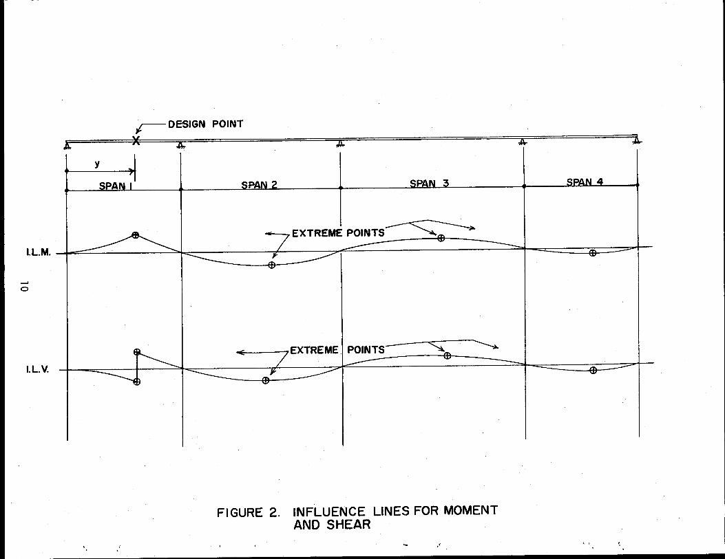
(!) and a train of arbitrarily spaced wheels (axle train). Fig. 2 shows

influence lines for moment and shear for a design point located in the

first span. Within each span, both the influence line for moment and for

shear will contain an extreme point (either a relative maximum or relative

minimum). In seeking the position of series of moving wheel loads which

produces either an absolute maximum or minimum value of moment or shear,

one need consider only those positions where an extreme point is contained

between the first and last wheels in the series. These limiting positions

are shown in Fig. 3 for the first extreme point on the moment influence

line for an axle train moving from left to right across the bridge. The

magnitude of the moment produced at the design point by a series of wheels

is obtained by multiplying the weight of each wheel times the ordinate of

the moment influence line beneath that wheel, and summing the results over

all wheels in the series. A relative maximum value of moment at the

9

r- DESIGN POINT

A X ~ A f ~ y

SPA

EXTREME POINTS~ -I.L.M. I ===-====== ~0:::::::::::::: ,/ ~ r-===== ~ (f) ::::::="" I -' 0

I. LV.

FIGURE 2. INFLUENCE LINES FOR MOMENT AND SHEAR

.•

·.

design point will occur for some intermediate position of the wheel series

lying between the starting and terminal positions shown in Fig. 3. The

position for maximum moment can be found in an efficient manner by sequen­

tially moving the leading wheel (W1 in Fig. 3) from its starting to

terminal position and computing the moment for each move. Once the trailing

wheel (W4 in Fig. 3) has reached its terminal- position, the wheel series

"skips" to the starting position for the next extreme point on the influence

line. This procedure is repeated until the last extreme point is traversed

and then the process is repeated, with the wheel series moving from right

to left, beginning at the right - most extreme point. An inspection of

the relative maximum and minimum values of moment obtained for each extreme

point produces the absolutely largest and smallest (most negative) values

of moment at the design point. The largest and smallest values of shear

force at the design point are obtained by the same procedure.

A slight variation on this method is necessary to accommodate the

AASHTO HS-truck, which has a variable wheel spacing. For each position of

the leading wheel w1, the spacing of the rear wheels w2 and w3 must be

varied )between the limits of 14 and 30 ft to find the relative maximum

moment for that leading wheel position. The terminal position of the HS­

truck is reached when the rear wheel w3 is over the influence line

extreme point and the rear wheel spacing is 30ft. These limiting positions

are shown in Fig. 4 for an HS-truck moving from left to right.

2.3 Maximum and Minimum Values for Moment and Shear - Lane and Uniformly Distributed Loads ·

Influence lines for shear and moment may be integrated to compute the

shear or moment at a design point produced by a uniform load. For uniformly

11

_rDESIGN POINT

SPAN I

w4 w3 W2 w

1 __, N

w4 w3.

I.L.M.-}c===========--------------------==========~L--

•. ,'

FIGURE 3. START AND TERMINAL POSITIONS FOR AXLE TRAIN AT EXTREME POINT I

·'

__, w

,· ·. ... .,

. r DESIGN POINT

4 A ~ T

w3 w3 w2 I I I I I W1 I I

STARTING POSITION I I FOR HS-TRUCK I J 14ft. t 14ft. l

30ft. . . 14ft

TERMINAL POSITION FOR HS-TRUCK

1

w3 w2

30ft.

FIGURE 4. STARTING AND TERMINAL CONFIGURATIONS FOR HS- TRUCK

distributed loads extending over the entire beam, the total area under

the curves in Fig. 2, scaled by the magnitude of the uniform load, will

give the moment and shear at the design point. With AASHTO lane loading,

partial spans may be loaded to produce maximum effects. In Fig. 2, inte­

gration should be carried over spans 1 and 3 to produce maximum at the

design point. In general, the maximum and minimum values of moment and

shear are obtained by summing all positive or negative areas beneath the

curves, respectively. Lane loadings also include an additional concen­

trated force (two in the case of negative moment) positioned to produce

maximum effect. The position of the concentrated force can be determined

from inspection of the ordinates of the influence lines. The requisite

integrations can be executed numerically since ordinates of the influence

lines are known at discrete points along the span.

2.4 Moments and Shears Produced by Dead Load

Dead load moments and shears are produced by the weight of the beams

themselves, diaphrams and deck slab. The moments and shears due to beam

weight are computed in the usual manner. The forces resulting from

diaphrams is computed from simple beam theory, based on their number and

spacing input to the program.

Forces resulting from the weight of the slab depend on deck place­

ment sequence. The program computes moments and shears due to the place­

ment of slab segments over supports for continuity, using simple beam

theory. Forces resulting from the placement of the remainder of the

deck utilizes numerical integration of the influence lines as described

above.

14

'

.·

·.

III. CREEP AND SHRINKAGE RESTRAINT FORCE COMPUTATIONS . '

The manner in which restraint forces are created in a continuous

beam can be visualized as those forces necessary to re-establish continuity

when each span of the beam is allowed to deform without restraint.

Figure 5(a) and (b) shows a prestressed beam immediately after placement

on its supports and at some later period after creep has occurred.

Hith the passage of time, the simple beam will continue to deform from

its initial position. Two opposing effects are at work; creep under

dead weight stresses which tend to sag the beam downward, and creep

under prestress forces which tend to camber the beam upward. The latter

effect dominates for the situation shown in Fig. 5. The two simple

beams are not free to deform independently as shown, because continuity

is established at the outset. The moment that would exist at some time

t, assuming that no stress redistribution was produced in the beam by

creep, is that moment necessary to establish continuity of slope (the

angles e in Fig. 5) at the supports. Obviously, stress redistribution

does occur as the result of creep, and the true final restraint moments

at time t are obtained from scaling the moments which re-establish

continuity by (~)

SFcreep = 1!q,

where

Ec =creep strain at timet due to unit stress,

Ee = initial strain due to unit stress, and

a = fraction of E which has occurred when continuity connection is established.

15

( 18)

( 19)

(a) INITIAL DEFORMATION

M1

I {c) RESTORATION OF CONTINUITY

ld) CREEP RESTRAINT MOMENT DIAGRAM

FIGURE 5. CREEP RESTRAINT MOMENT

16

.~

The end result is a linearly varying moment superimposed on those

described in the previous section. The creep restraint moments may be

either positive or negative, depending on the amount and location of

prestressing.

Figure 6 indicates the deformation produced by differential

shrinkage between slab and beam concrete. When the deck is cast, a

substantial portion of the shrinkage in the beams has already occurred.

Thus, the shrinkage rate in the slab is more rapid, and overruns the

rate of shrinkage of the beams. The result is an overall compression

of the top of the beams, where they interface with the deck, which

produces downward deflection. The final moments which occur in the

beam as a result of its continuity are the moments necessary to re-

establish continuity, scaled by (_g)

1 SFshrinkage = 1+~

where~ is defined by Eq. (19).

3.1 Computation of Unsealed Restraint Moments

(20)

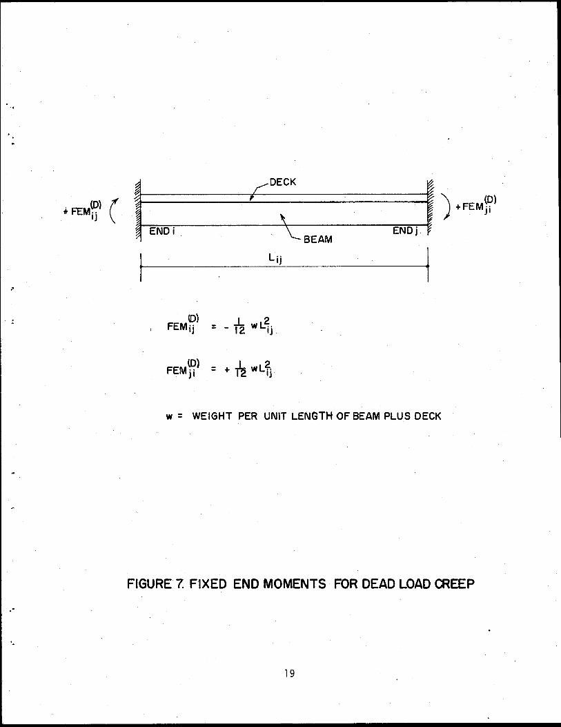
The unsealed restraint moments produced by shrinkage and dead load

and prestress creep are computed by the slope-deflection method of

elastic analysis. The fixed end moments for span (i ,j) of the continuous

beam are denoted by FEM .. and FEM ... Positive fixed end moments are lJ Jl those which tend to rotate the support in a counterclockwise direction.

Expressions for the fixed end moments from each of the three restraint

moment sources are given in Figs. 7 through 9.

17

r------------------

(a) INITIAL DEFORMATION

I (b) DEFORMATION AT TIME t

1tr1i ~r=::=.========~ ~~q_

~ M2 I

(c) RESTORATION OF CONTINUITY.

(d) SHRINKAGE RESTRAINT MOMENT DIAGRAM

FIGURE 6. SHRINKAGE RESTRAINT MOMENTS

18

~ rOECK :;-

,t FEM~~) ( ~ ,

) + FEM~~) IJ ~ \

J I

~ ENOi \._BEAM

ENOj

Lij j ..

1 (D) j_ 2 FEMij = - 12 wl..!ij

FEM~) = + 12 wL~· Jl IJ .

w = WEIGHT PER UNIT LENGTH OF BEAM PLUS DECK

FIGURE 7. FIXED END MOMENTS FOR DEAD LOAD CREEP

.·

·.

19

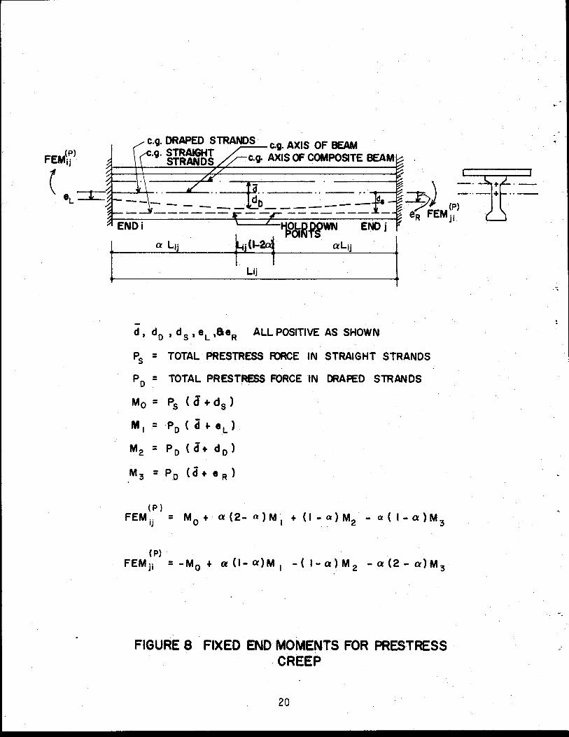
e.g. DRAPED STRANDS e.g. AXIS OF BEAM e.g. STRAIGHT e.g. AXIS OF COMPOSITE BEAM

STRANDS

d, d0 , ds, eL ,&eR ALL POSITIVE AS SHOWN

P5 = TOTAL PRESTRESS FORCE IN. STRAIGHT STRANDS

P 0 = TOTAL PRESTRESS FORCE IN DRAPED STRANDS

Mo = P5 ( d + ds )

M 1 P0 ( d .. eL)

M2 =P 0 (d+d 0 )

M 3 = Po ( d + e R )

( p)

FEMij = M0 + a(2- a)M 1 + (1-a)M2

- a( l-a)M3

( P) FEMji =-M0 + (r(l-a)M 1 -(1-a)M 2 -a(2-a)M 3

FIGURE 8 FIXED END MOMENTS FOR PRESTRESS CREEP

20

.·

·~

+FEM~~l IJ

( e · C e.g. a= coMPOsT£ BEAM )(!I

3------------------~ +FEMji £NDi END j

! FEM (~ = ·. iJ

(S) FEM ji = 'soEAe

• SO= DIFFERENTIAL SHRINKAGE STRAIN 8ETWEEN DECK AND BEAM CONCRETE (see Section 3.2)

E = MODULUS OF ELASTICITY OF DECK CONCRETE

A = CROSS SECTIONAL AREA OF DECK

e = DISTANCE BETWEEN MID DEPTH OF DECK AND CENTROID OF·COMPOSITE SECTION

FIGURE 9. FIXED END MOMENTS FOR SHRINKAGE

21

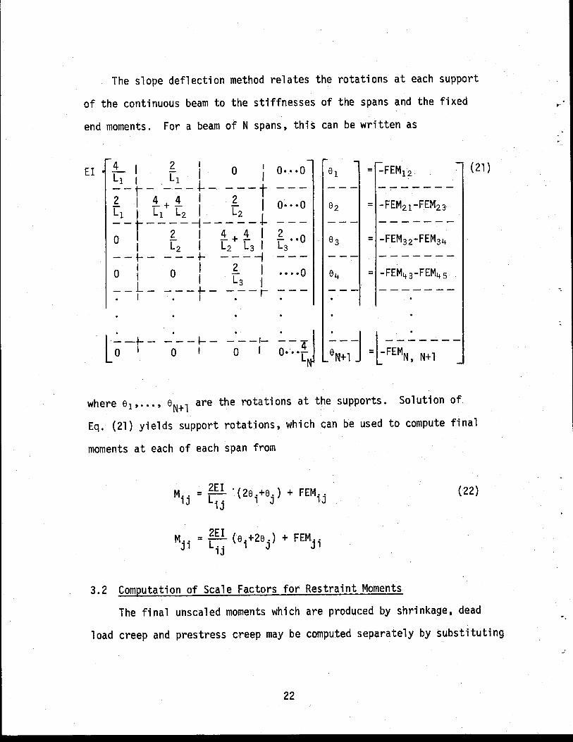
The slope deflection method relates the rotations at each support

of the continuous beam to the stiffnesses of the spans and the fixed

end moments. For a beam of N spans, this can be written as

EI 4 I 2 0 0· •• 0 el -FEM12 (21) I7

= I l1

--~- ---+-- ---t --- --- -------.£ I .1.+.1. I .£ I 0·. ·0 62 = -FEM21-FEM23 Ll I Ll L2 I L2 ~-~--.?. -~--4-+-4-t --- --- -------

2 -FEM32-FEM3'+ - • ·0 63 = I l2 I l2 l3 I L3

--t-- ---.J- -----1 --- --- -------0

I 0 I 2 I •••• 0 -FEM43 -FEM45 I I [3 e'+ =

I ..

__ L_ ---.J-- ---r --- --- -------

I I

l ~ -r - -~- -i - ___ ,_ 0 I

where e1 , ••• , eN+l are the rotations at the supports. Solution of

Eq. (21) yields support rotations, which can be used to compute final

moments at each of each span from

M .. = ~EI '(2e .+e.) + FEM .. 1J ij 1 J 1J

2EI M. . = -L - (e. +2e . ) + FEM .. J1 . . 1 J J1

1J

3.2 Computation of Scale Factors for Restraint Moments

(22)

The final unsealed moments which are produced by shrinkage, dead

load creep and prestress creep may be computed separately by substituting

22

";

•

. ·

the appropriate fixed end moments into Eqs. (21) and (22). The resulting

moments are scaled by the shrinkage and creep factors given in Eqs.

(18), (19) and (20) and summed to give the final restraint moments.

The scale factors in Eqs. (18) and (20) depend on the creep factor

~'which is defined by Eq. (19). To determine~' one must have a unit

creep curve for the beam and deck concrete (the deck and beam concretes

are assumed to have the same creep and shrinkage behavior) to establish

ec. Previous research has been conducted on the creep and shrinkage

of concretes typically used by the Texas Highway Department for pre­

stressed beams (1). Creep and shrinkage data were taken on concretes from

four localities in Texas, and the properties of these concretes are

listed in Table 1. Studies on creep and shrinkage were conducted on

3 in. x 3 in. x 16 in. prisms stored under laboratory conditions of

50% humidity and 73°F. Expressions which were found to fit the shrinkage

and unit creep strain data are listed in Table 2. A reasonable estimate

of the overall average ·unit creep function ec(t) and shrinkage strain

function es(t), applicable for all locations, is given by

ec(t) = 425t (in./in./ksixl0- 6) 34+t

( ) 525t (' /' 10-6) es t = 20+t 1n. 1n.x

(23)

(24)

where the constant terms in each expression are the average of those

values appearing in Table 2. The value for ec appearing in Eq. (19)

should correspond to the maximum unit strain expected for any time t .

23

Measured Computed* Release Strength Release Modulus Release Modulus

Location (psi) (ksi) ( ksi)

Dallas 7,080 5,200 4,800

Odessa 5,050 3,260 4,050

San Antonio 5,250 4,220 4,130

Lufkin 5,760 4,440 4,330

* Using ACI 318-71 Equation, E = 57,000 Jf7 c

Location

Dallas

Odessa

San Antonio

Lufkin

TABLE 1. STRENGTH AND MODULI VALUES FROM REFERENCE (1)

Shrinkage _6

Creep (in./in. x 10 ) (in./in./ksi x 10-6

)

SOOT* 365T lS+T 40+T

650T 525T 20+T 25+T

SOOT 385T 20+T 25+T

450T 430T 25+'F 45+T

* T-time in days

TABLE 2. EXPRESSIONS FOR SHRINKAGE STRAIN. AND UNIT CREEP STRAIN FOR 3 in. x 3 1n. x 16 in. PRISMS STORED UNDER LABORATORY CONDITIONS (From Reference 3)

24

~

-·

...

·-

This will occur, according to Eqs. (23), ~hen t = oo and yields sc = 425

(in./in./ksixl0- 6). This basic unit creep strain is for concrete

specimens with a volume/surface ratio of approximately 1.0, loaded at

approximately 1 day after casting, and cured under a constant relative

humidity of 50%. Corrections to the basic unit creep strain are required

for volume/surface ratios significantly different from 1.0. The age of

the test specimens at loading is representative of the production sequence

used by most manufacturers, so no correction is applied for age at loading.

The modified unit creep strain €c is written as

(25)

where av/s is the correction to the basic unit creep strain. A plot of

this correction factor versus volume/surface ratio is given in Fig. 10.

It was obtained by downward shift of a similar curve appearing in

reference (i), so that av/s = 1.0 for the volume/surface ratio of 1.0

at which the creep data were taken. Noting that ~ in Eg. (19) is given by

1 425t t a = 425 • 34+t = 34+t (26)

that

(27)

and that Eq. (25) gives the corrected unit creep strain, we have

(28)

25

1.0

..(!! >

C$ 0.9 ~

~ 0 ~ z 0

0.8 ~ 0 w et: ~ 0 0

0 0.7 t-<( a: w 0

~ ~ 0.6 ::::> en ....... w :E ~ ...J 0 >

0.5

~ \

1.0

\

1\ \ ~ ~ !'-..

............

I'--~

5.0 VOLUME I SURFACE RATIO (in)

FIGURE 10. SHRINKAGE STRAIN CORRECTION FACTOR

26

·-.

---r-----

10.0

-·

.-

·-

where

Ei = modulus of elasticity of beam concrete at release of strands (ksi),

t =age of.the beam in days, when continuity connection made, and

av/s = correction factor from Fig. 10.

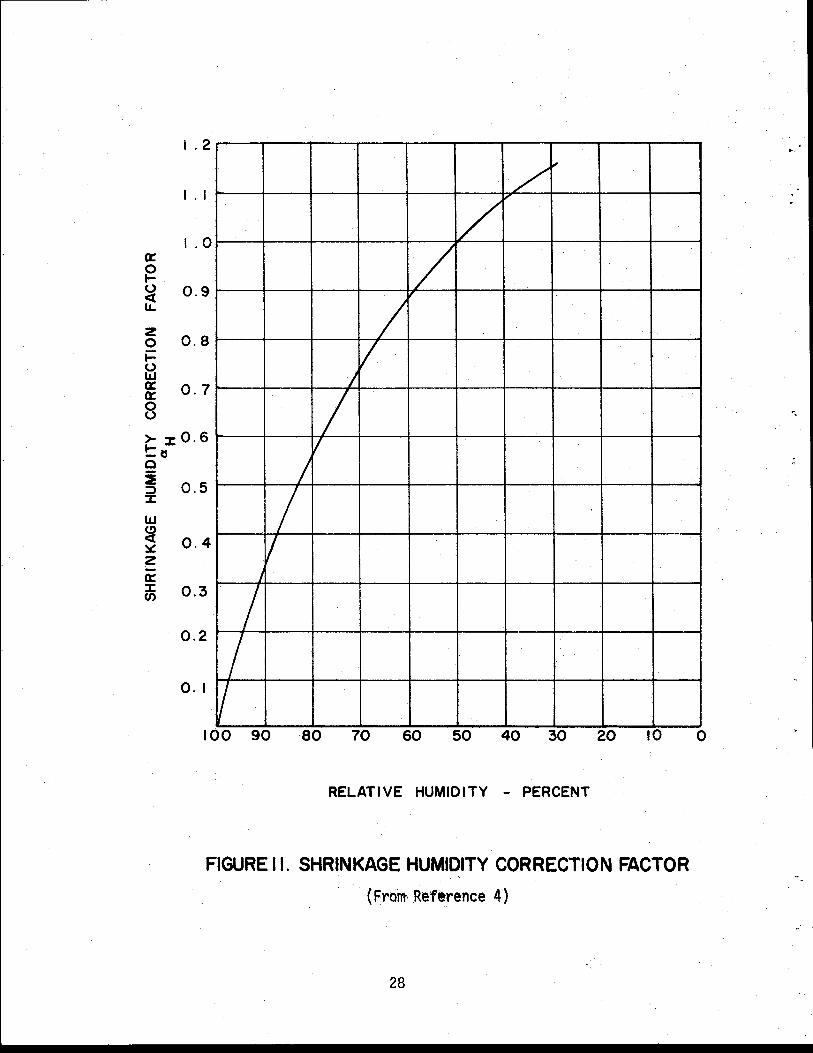
Corrections to the ultimate shrinkage strain of 525 (in./in.xl0-6

)

(obtained from Eq. (24) with t = oo) must be made for relative humidities

greatly different from 50%. Letting esu be the corrected ultimate

shrinkage strain, we have

(29)

where aH is a humidity correction factor taken from reference (i), and

shown in Fig. 11. The differential shrinkage strain eSD used in Fig. 9

for the computation of fixed end moments due to shrinkage can be written

as

(30)

The factors is the fraction of shrinkage which has occurred in the beam

concrete before the deck is cast. From Eq. (24),

( 31)

Substituting Eqs. (29) and (31) into (30) gives

(32) I

27

I. 2

I . I

I .0 a:: 0 1-u 0.9 <X IJ.

z 0 0.8 i= ~ ~ 0. 7

8 > J: 0. 6 t:a 0 i ::) 0.5 J:

w ~ 0.4 ~ z -a:: :J: 0.3 Cl)

0.2

0. I

/'

/ /

I v I

I v

I I

I I

I I I

I 00 90 80 70 60 50 40 30 20 I 0 0

RELATIVE HUMIDITY - PERCENT

FIGURE II. SHRINKAGE HUMIDITY CORRECTION FACTOR

( Fro!ll' Re'ference 4)

28

·.

where

aH =correction factor from Fig. 11, and

t = age of beam concrete when deck cast.

Thus, the final scaled restraint moments may be obtained by performing

the elastic analysis described previously (using Eq. (32) to obtain shrinkage

fixed end moments), computing the creep factor from Eq. (28) and scaling

the moments resulting from prestress and dead load creep by Eq. (18) and

from shrinkage by Eq. (20).

29

IV. DESIGN CRITERIA

The computer program developed in this study carries out the design

of a continuous beam constructed with precast, prestressed concrete I-

beams. The applicable design code is Standard Specifications for Highway

Bridges, 11th edition, published by The American Association of State

Highway and Transportation Officials (l_). This section reviews the

provisions of this Specification which govern the design and outlines

the computations made in arriving at a satisfactory design. In the

following discussion, reference to a "Section" denotes a provision from

this document.

4.1 Predesign Decisions

The structural engineer, charged with the responsibility for the

complete design of a bridge, can utilize this program to carry out

routine computations involved in selection of strand patterns, longi­

tudinal deck reinforcing, stirrups, and continuity connection reinforce-

ment. To interface with the program, he must first specify:

(i) the length.of each span in the continuous beam,

(ii) the geometrical properties of the precast beam (which must be the same for all spans),

(iii) the properties of reinforcement, beam concrete and slab concrete,

(iv) the beam spacing,

(v) the slab thickness,

(vi) the design live load, and

(vii) the type of continuity construction {partially continuous for dead load or continuous for live load only}.

30

>·

•.

•'

The program contains a greatly simplified input format to accommodate

designs which incorporate standard THO and AASHTO beams, reinforcement

and loadings. The details of program input are explained in Vol. II of

this report.

4.2 Beam Design Loads

from

The live load moments and shears used in design can be computed

(i) standard AASHTO trucks and lane loadings,

(ii) a series of up to 15 arbitrarily spaced, moving wheels "axle train",

(iii) a uniformly distributed live load applied to the continuous beam and superimposed on the load produced by (i) or (ii).

The portion of an AASHTO truck and lane loading applied to the beam

is determined from Section 1.3.1 and taken as S/5.5, unless specified

otherwise on the input form. The fraction of wheel loads from an axle

train which is applied to the beam is specified on input. No lateral

distribution of uniform load is included in the program.

Dead load moments and shears from beam weight, diaphrams and

portions of the deck poured for continuity are computed from input

information.

31

4.3 Criteria for Strand Pattern Selection

Strand pattern selection for a span of the continuous beam is

based primarily on service load stress considerations, although ul­

timate strength requirements may in some cases govern strand placement.

In each span, stresses produced by loads are checked at top and bottom

of the beam at tenth points (each end and 9 interior points). Stresses

produced by prestress at strand release are checked at top and bottom

of beam, at each end and hold down points. Hold down points vary with

span length and are listed in Table 3.

4.3.1 Calculation of Load Induced Stresses - Four stress checks

are made at each tenth point during strand placement, as indicated in

Table 4. Stress produced by external loads at the top and bottom of a

beam at the ith tenth point are given by

where

+ MRi}

= 1 {M(B) + M(DNC)} 0 bi rb Dli Dli

+ MRi}

1 + zc.

t

1 + zc

b

Zt = top section modulus of beam,

{ (DC)

MDLi + (MLLi + I)

{ (DC)

MDLi + (MLLi + I)

Zb = bottom section modulus of beam,

zct = top section modulus of composite beam,

ZCb = bottom section modulus of composite beam,

M~~~= moment at ith tenth point due to beam weight,

32

(33)

(34)

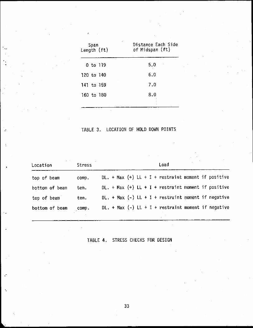
Span Distance Each Side Length (ft) of Midspan (ft)

0 to 119 5.0

120 to 140 6.0

141 to 159 7.0

160 to 180 8.0

.~ TABLE 3. LOCATION OF HOLD DOWN POINTS

Location Stress Load

top of beam camp. DL. + Max ( +) LL + I + restraint moment if positive

bottom of beam ten. DL. + Max ( +) LL + I + restraint moment if positive

top of beam ten. DL. + Max (-) LL + I + restraint moment if negative

bottom of beam camp. DL. + Max (-) LL + I + restraint moment if negative

TABLE 4. STRESS CHECKS FOR DESIGN

·.

33

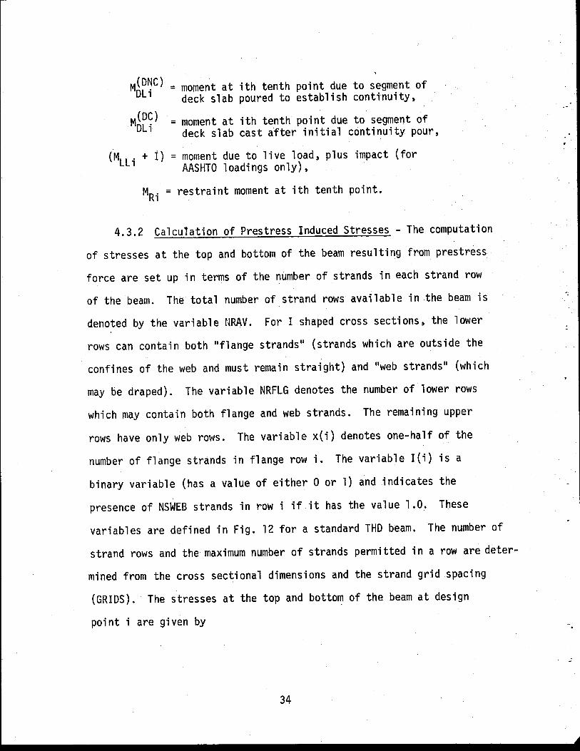
M~~~C) = moment at ith tenth point due to segment of deck slab poured to establish continuity,

M(DC) Dli

= moment at ith tenth point due to segment of deck slab cast after initial continuity pour,

(MLLi + i) =moment due to live load, plus impact (for AASHTO loadings only),

MRi = restraint moment at ith tenth point.

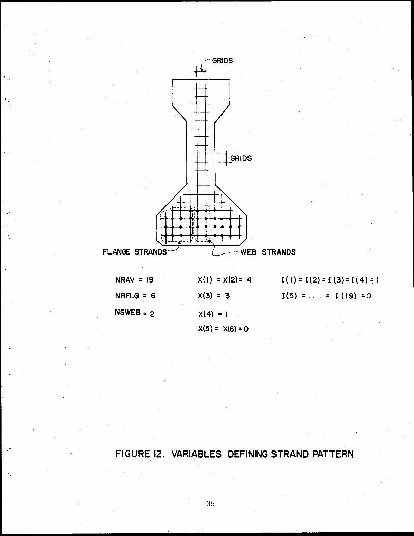
4.3.2 Calculation of Prestress Induced Stresses - The computation

of stresses at the top and bottom of the beam resulting from prestress

force are set up in terms of the number of strands in each strand row

of the beam. The total number of strand rows available in the beam is

denoted by the variable NRAV. For I shaped cross sections, the lower

rows can contain both 11 flange strands 11 (strands which are outside the

confines of the web and must remain straight) and 11Web strands'' (which

may be draped). The variable NRFLG denotes the number of lower rows

which may contain both flange and web strands. The remaining upper

rows have only web rows. The variable x(i) denotes one-half of the

number of flange strands in flange row i. The variable I(i) is a

binary variable (has a value of either 0 or 1) and indicates the

presence of NSWEB strands in row i if it has the value 1.0. These

variables are defined in Fig. 12 for a standard THO beam. The number of

strand rows and the maximum number of strands permitted in a row are deter­

mined from the cross sectional dimensions and the strand grid spacing

(GRIDS). The stresses at the top and bottom of the beam at design

point i are given by

34

-.

.-

NRAV = 19

NRFLG = 6 .

NSWEB: 2

~RIDS

X(l) = X(2) = 4

X(3) = 3

X(4) = I

X(5) = X(6) = 0

STRANDS

I ( I} = 1( 2) = I ( 3) = l ( 4} = I

1(5) = ... = 1 ( 19) = 0

FIGURE 12. VARIABLES DEFINING STRAND PATTERN

35

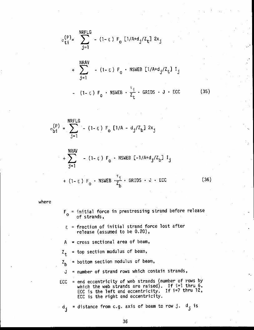
NRFLG ai~)= L -(1- ~) F 0 [1/A+d/Zt] 2xj

j=l

NRAV + L -( 1- ~ ) F 0 • NSWEB [ 1 I A+d /Zt] I j

j=l

T •

- ( 1- ~ ) F0

• NSWEB • 1 • GRI OS • J • ECC ( 35) zt

NRFLG (P) = " 0 bi £..J

where

j=l

NRAV + L - (1- ~) F 0 • NSWEB [-1/A+d/Zb] Ij

j=l

T •

+ ( 1- ~ ) F • NSWEB ·-1 • GRIDS • J • ECC o zb

(36)

F0

= initial force in prestressing strand before release of strands,

~ = fraction of initial strand force lost after release (assumed to be 0.20),

A = cross sectional area of beam,

Zt = top section modulus of beam,

Zb = bottom section modulus of beam,

J = number of strand rows which contain strands,

ECC = end eccentricity of web strands (number of rows by which the web strands are raised). If i=l thru 6, ECC is the 1 eft end eccentricity. If i =7 thru 12, ECC is the right end eccentricity.

dj =distance from e.g. axis of beam to row j. dj is

36

--

.-

·-

positive if row j is above the e.g. axis,

l {a-i/10); 0~ iL/lO~aL a

T i = 0 ; al <i L/ 1 O<L ( 1-a) l (i/10-a); L(l-a)<iL/lO<L, and a -

a, L = defined in Fig. 8.

4.3.3 Selection of Number and Positions of Strands - A trial strand

pattern is selected based on tension stress at the bottom of the beam at

the tenth point where maximum positive moment occurs. The end eccentricities

are assumed to be zero during strand pattern selection. The allowable

tensile stress is taken as

crten = 6.0 ~ (37)

where f~ is the minimum 28 day strength of the beam concrete, specified

on input. The total stress at the bottom of the beam is the sum of those

stresses given by Eqs. (34) and (36).

The strand pattern selection proceeds with sequential placement of

strands in each row. NSWEB strands are first placed in row 1, (I 1 = 1),

followed by placement in pairs of flange strands (x1). If additional

strands are required, the sequence of events is repeated for higher rows,

until the final tension stress in the bottom of the beam is less than that

given by Eq. (37).

After an initial pattern of strands has been selected, cracking and

ultimate moment capacities of the section are computed. If the ultimate

moment is less than 1.2 times the cracking moment, additional strands are

added, by the same process described above, until this code provision (Section

1.6.10 (B)) is met.

37

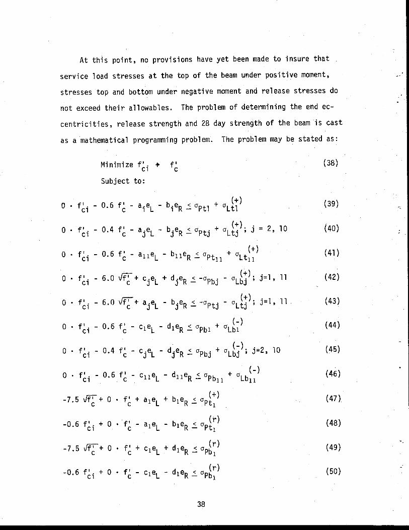
At th1s point, no provisions have yet been made to insure that

service load stresses at the top of the beam under positive moment,

stresses top and bottom under negative moment and release stresses do

not exceed their allowables. The problem of determining the end ec­

centricities, release strength and 28 day strength of the beam is cast

as a mathematical programming problem. The problem may be stated as:

Minimize f~i + f' c Subject to:

0 • f'. - 0.6 f' - aiel - bieR 2 °Ptl (+)

Cl c + 0 L tl

0 • f'. - 0 6 f' - alleL - blleR ~ crPtll + cr (+)

Cl . c Lt11

0 • f'. - 6.0 Vfl + c.el + d.eR < -crPb" ( +). j=l ' 11

Cl c J J - J -0 Lbj '

0 • f'. - 6.0 ~+ a.el- b.eR < -crPt" (+). j=1' 11

Cl c J J - J -0 Ltj '

0 • f'. - 0 6 f' (-) Cl . c - cleL - d1 eR ~ 0 Pbl + 0 Lbl

0 • f~i - 0.4 f~- cjel - djeR ~ crPbj + crl~j); j=2, 10

0 • f~i - 0.6 f~ - c11 el - d11 eR ~ crPb11

+ crlb~~)

0 6 f • + 0 f' b (r) - . ci • c - aleL - leR ~ crPtl

-7.5 Jf~ + 0 f~ + c1el + d1eR 2 crp~:)

0 6 f • + 0 f' ~ c e d e (r) - ' ci • c 1 L - 1 R ~ 0 Pb 1

38

(38)

(39)

(41)

(42)

(43)

(44)

(45)

(46)

(47)

(48)

(49)

(50)

-7.5 ~ + 0 • f' + a11 eL + b11 eR < crPt(r) C1 C - ll

-0.6 f'. + 0 • f' - a11 eL - b11 eR < crPt(r) C1 C - ll

-7.5 ~ + 0 • f' + c11 eL + d11 eR < crPb(r) C1 C - ll

-0.6 f~i + 0 • f~ - 0 • eL - 0 • eR ~ crpi~)+ crwth

-7.5 /f~i + 0 • f~ + 0 • eL + 0 • eR ~ crp~~)- crwbh

-0.6 f'. C1

+ 0 . f' + 0 . eL + 0 . eR :: crPbh + crwbh c

eL ~ emax

e < e R - max

-f'. < -4.0 C1

-f' < -5.0 c

f'. -f' < 0.0 C1 c -

where

f~i = release strength,

f~ = 28 day strength,

eL = strand eccentricity at left end of beam,

e = strand eccentricity at right end of beam, R T •

a. - - (1-t;) F • NSWEB • f · GRIDS • J J 0 -t

b. - - (1-l;) • F J 0

NSWEB • T. _1_. zt

GRIDS • J

~9

(51)

(52)

(53)

(54)

(55)

(56)

(57)

(58)

(59)

(60)

(61)

(62)

(63)

1".

c. = (1-1;) . Fo • NSWEB • zl · GRIDS • J J b

-1" •

d. = (1-1;) • F • NSWEB • zL · GRIDS • J J 0 b

= l (a-j/10); .L

1" • 0 ~ m ~ al J a

0 ; 'L

al ~ tij- ~ L

'L 1'· =

J 0 ; 0 ~ fij ~ L(l-a)

1 . .L ~ (J/10-l+a); L(l-a) ~ 1o ~ L

= stress top and bottom of beam at jth tenth point, respectively, due to prestress and computed from Eqs. (35) and (36) .with the omission of the last term in each of these equations,

(+) (+)_ crltj + crlbj - stress top and bottom of beam at jth tenth point produced by dead load moment, positive live load moment and creep restraint moment, if positive,

al~;)+ cr~~J = stress top and bottom of beam at jth tenth point produced by dead load moment, negative live load moment and creep restraint moment, if negative,

stress top and bottom of beam at jth tenth point (j=l is left end, j=ll is right end and j=h is hold down point) due to prestress at release, computed from Eqs. (35) and (36) with the omission of the last term in each of these equations,

crwth + crwbh = stress top and bottom of beam at hold down point produced by beam weight, and

e = maximum number of rows that web strands may be max raised at end of beam (depends on J, the number

of rows with strands).

This problem contains four variables (f~i' f~, eland eR) and 61

inequality constraints (Eqs. 39 thru 63). The constraints are linear

with the exception of those containing ~ or ~. These are

40

·-

•

•

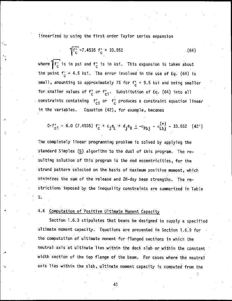
linearized by using the first order Taylor series expansion

~=7.4535 f~ + 33.552 (64)

where~ is in psi and f~ is in ksi. This expansion is taken about

the point f~ = 4.5 ksi. The error involved in the use of Eq. (64) is

small, amounting to approximately 7% for f~ = 9.5 ksi and being smaller

for smaller values off~ or f~i· Substitution of Eq. (64) into all

constraints containing f~i or f~ produces a constraint equation linear

in the variables. Equation (42), for example, becomes

The completely linear programming problem is solved by applying the

standard Simplex (i) algorithm to the dual of this program. The re­

sulting solution of this program is the end eccentricities, for the

strand pattern selected on the basis of maximum positive moment, which

minimizes the sum of the release and 28-day beam strengths. The re­

strictions imposed by the inequality constraints are summarized in Table

5.

4.4 Computation of Positive Ultimate Moment Capacity

Section 1.6.3 stipulates that beams be designed to supply a specified

ultimate moment capacity. Equations are presented in Section 1.6.9 for

the computation of ultimate moment for flanged sections in which the

neutral axis at ultimate lies within the deck slab or within the constant

width section of the top flange of the beam. For cases where the neutral

axis lies within the slab, ultimate moment capacity is computed from the

41

~ N

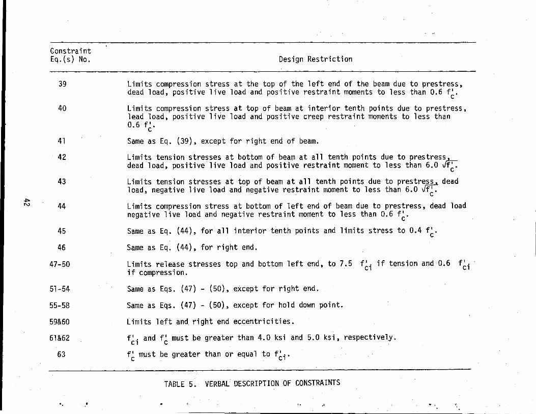
Constraint Eq. (s) No.

39

40

41

42

43

44

45

46

47-50

51-54

55-58

59&60

61&62

63

...

Design Restriction

Limits compression stress at the top of the left end of the beam due to prestress, dead load, positive live load and positive restraint moments to less than 0.6 f•. c

Limits compression stress at top of beam at interior tenth points due to prestress, lead load, positive live load and positive creep restraint moments to less than 0.6 f~.

Same as Eq. (39), except for right end of beam.

Limits tension stresses at bottom of beam at all tenth points due to prestress dead load, positive live load and positive restraint moment to less than 6.0 Jf~.

Limits tension stresses at top of beam at all tenth points due to prestrjss, dead load, negative live load and negative restraint moment to less than 6.0 f~.

Limits compression stress at bottom of left end of beam due to prestress, dead load negative live load and negative restraint moment to less than 0.6 f~.

Same as Eq. (44), for all interior tenth points and limits stress to 0.4 f~.

Same as Eq. (44), for right end.

~imits rele~se stresses top and bottom left end, to 7.5 f~i if tension and 0.6 1f compress10n.

Same as Eqs. (47) - (50), except for right end.

Same as Eqs. (47) - (50), except for hold down point.

Limits left and right end eccentricities.

f~i and f~ must be greater than 4.0 ksi and 5.0 ksi, respectively.

f~ must be greater than or equal to f~i·

TABLE 5. VERBAL DESCRIPTION OF CONSTRAINTS

• .. ...

f•. Cl

•,

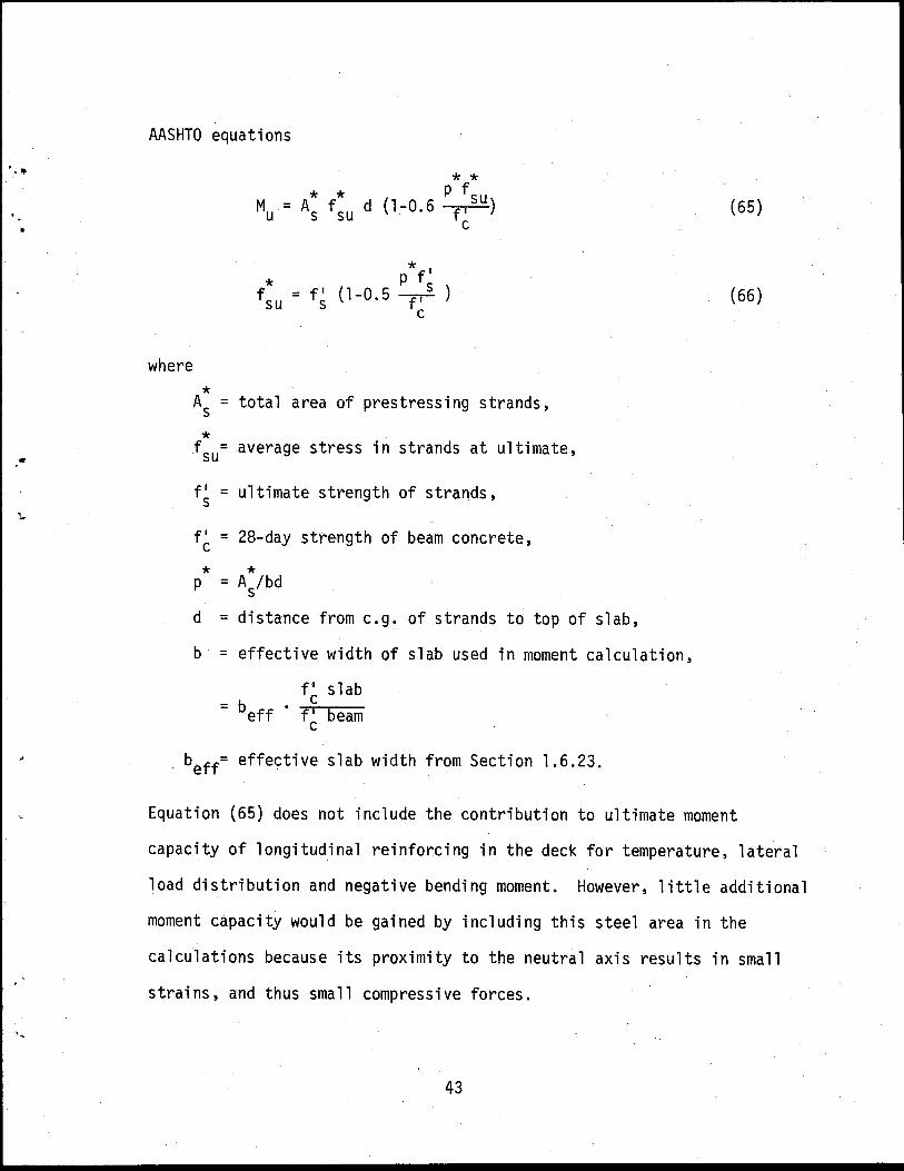
AASHTO equations

where

* * * * P fsu Mu = A f d (1~0.6 f• ) s su c

* p fl = f• (1-0.5 ----f.s

s c

* As = total area of prestressing strands,

* fsu= average stress in strands at ultimate,

f 1 = ultimate strength of strands, s

f~ = 28-day strength of beam concrete,

* * p = As/bd

d = distance from e.g. of strands to top of slab,

b = effective width of slab used in moment calculation,

f• slab c = beff • f• beam

c

beff= effective slab width from Section 1.6.23.

(65)

(66)

Equation (65) does not include the contribution to ultimate moment

capacity of longitudinal reinforcing in the deck for temperature, lateral

load distribution and negative bending moment. However, little additional

moment capacity would be gained by including this steel area in the

calculations because its proximity to the neutral axis results in small

strains, and thus small compressive forces.

43

For situations where the neutral axis lies in the beam, Eq. (65)

is not applicable. In addition, the stress in conventional reinforcing

in the deck slab will generally be at or near yield because of its

distance from the neutral axis. The calculation of ultimate moment

capacity when the neutral axis lies in the beam is therefore based on

the following assumptions:

(i) at failure, the compression strain at the top of the deck is .003 in./in.,

(ii) the strain profile is linear at ultimate,

(iii) the distribution of compression stress in the concrete can be replaced with the equivalent stress block shown in Figure 13, and the resultant compressive force in the concrete (C ) acts through the centroid of the area of the conErete under compression (shaded area in Figure 13),

(iv) the conventional reinforcing in the deck is assumed to be concentrated at mid-depth of the slab for calculation purposes, and its stress at ultimate is proportional to its strain up to the yield stress of 60 ksi and is constant thereafter,

(v) the average stress in the strands at ultimate is obtained from the stress-strain curve for the strands ·developed below.

The amount of reinforcing in the deck must be adequate to resist negative

moments produced by live loads and creep and shrinkage restraint moments.

The calculation of this required reinforcing area is described in the

next section. In addition, the AASHTO Specification requires certain

deck reinforcing for temperature and lateral load distribution. These

requirements are met by THO through the use of standard reinforcement

details for various beam spacings (~). The total area of reinforcing for

temperature and load distribution contained in the flange of the deck

44

..

•

...

.1

for various beam spacings is shown in Table 6, and were computed from

reference (~). The area of deck reinforcing used in the computation of

ultimate moment capacity when the neutral axis lies in the beam is the

greater of those areas required for negative moment at midspan and for

temperature and load distribution.

The stress-strain properties of the strands (assumption v above)

are assumed as:

Es = f /28,000; f < f 1 s- p (67)

f ~ (f' - f ) fQl (f~- fQ1)2 = Ql s Ql

Es 28 '000 l + ( f ~ 2fpl) - ( f l .:; 2f ) s pl

(68) 1 f.)) f > f 1

fs (f' s p s

where

Es = strain in the strand (in./in.)

fs = stress in the strand (ksi)

f' = ultimate strength of the strand ( ks i) s

fpl= proportional limit stress, assumed as 63 f' • s

Equations (67) and (68) are plotted for f~ = 250 and 270 ksi in Fig. 14.

The ultimate moment capacity of sections where the neutral axis falls

below the slab is given by

M = C • d + C • d' u c s (69)

where Cc' d, Cs and d' are defined in Fig. 13. The resultant compressive

forces Cc and Cs can be computed once the location of the neutral axis c

45

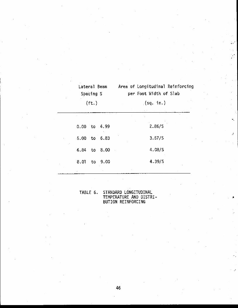
Lateral Beam Spacing S

(ft.)

0.00 to 4.99

5.00 to 6.83

6.84 to 8.00

8.01 to 9.00

Area of Longitudinal Reinforcing per Foot Width of Slab

(sq. in.)

2.86/S

3.57/S

4.08/S

4.39/S

TABLE 6. STANDARD LONGITUDINAL TEMPERATURE AND DISTRI­BUTION REINFORCING

46

...

·"'

.j::::o '-I

(

e.g. of strands

f 1c slab b = b ff• e f•c beam

)'

beff = effective slab width

Neutral XIS

d

J~ ·,

c E' ·s

Es

Strain Profile at Ultimate

T

Stress Profile at Ultimate

FIGURE 13. STRESS AND STRAIN PROFILES AT ULTIMATE FOR POSITIVE MOMENT

d dl

C' en

.X:

U) U)

w 0::: t-U)

300

250

200

150

100

50

0 o.o

\'" =270

--....... ---

v ~

~ f.,.---" ·~

I t• = 250 s

I

0.02 0.04 0.06 0.08

STRAIN (in/in)

FIGURE 14. STRESS- STRAIN CURVES FOR PRESTRESSING STRANDS

(A plot of Eqs. 67 & 68)

48

-\J

1''-

0.10

.. ,

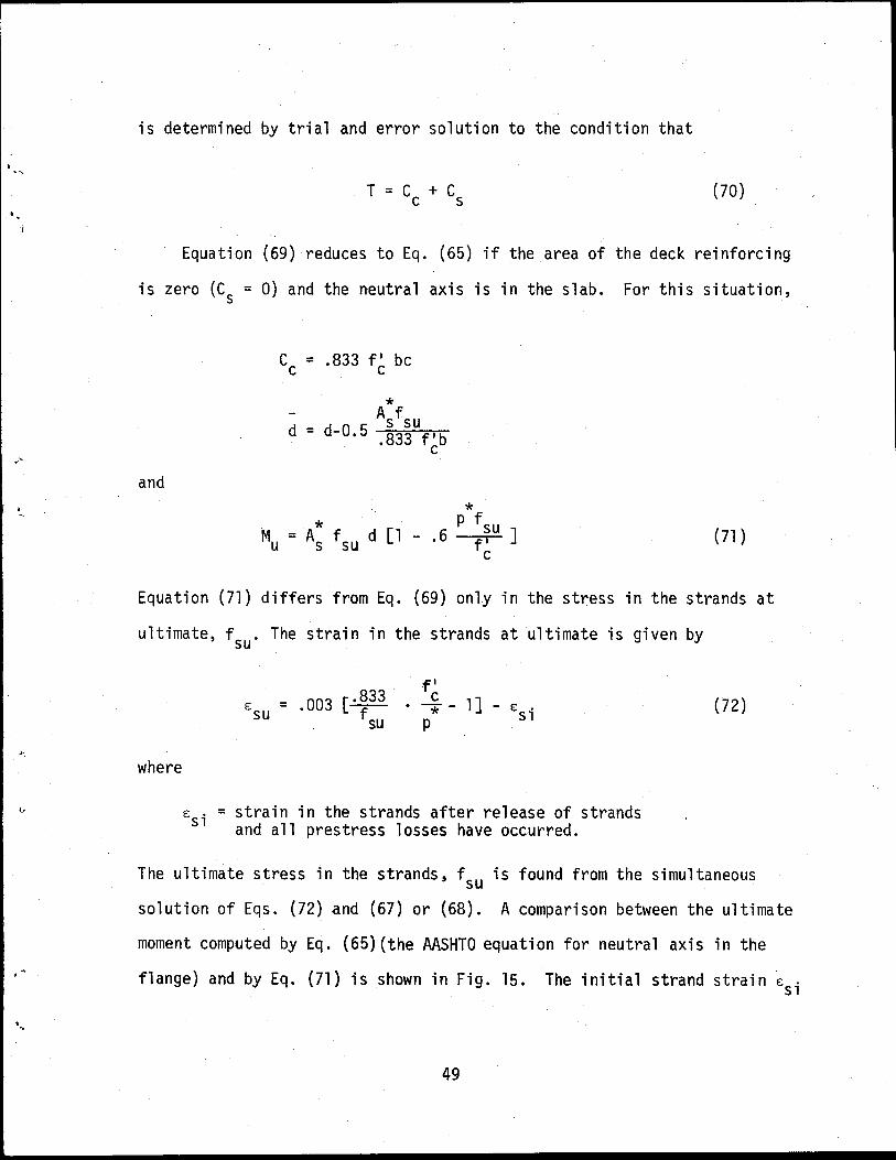
is determined by trial and error solution to the condition that

T = C + C c s

(70)

Equation (69) reduces to Eq. (65) if the area of the deck reinforcing

is zero (Cs = 0) and the neutral axis is in the slab. For this situation,

Cc = .833 f~ be

* - A f s su d = d-0·5 .833 f~b

and

(71)

Equation (71) differs from Eq. (69) only in the stress in the strands at

ultimate, fsu· The strain in the strands at ultimate is given by

where

E: • Sl

esu = • 003 [. 8f33 su

f' c . *-p

1] - E: • Sl

= strain in the strands after release of strands and all prestress losses have occurred.

(72)

The ultimate stress in the strands, fsu is found from the simultaneous

solution of Eqs. (72) and (67) or (68). A comparison between the ultimate

moment computed by Eq. (65)(the AASHTO equation for neutral axis in the

flange) and by Eq. (71) is shown in Fig. 15. The initial strand strain

49

E: • Sl

. 20

.16

-

FROf ~ EQS. (65) E (66) ( (AA~ HTO)

-~~ .......

1\ _,_:::::. P"'

rr ~ ~

~

.... v FRO ~ EQ (71), ~67),(68)

-7

.08

. 04

o.o .02 .04 .06 .08 0.10

p *f* su f I

c

FIGURE 15. COMPARISON OF MOMENT CAPACITIES FOR NEUTRAL AXIS IN SLAB

50

< •

,,

0.12

.. ·

. .,.

was taken as .00002 f~. For practical ranges of reinforcement index, the

two approaches give nearly identical results for cases where the neutral

axis lies in the slab.

4.5 Computation of Negative Moment Deck Reinforcement

Negative moments are produced in the continuous beam by live loads,

and in some cases, by creep restraint effects. Section 1.6.12(c) (3)

stipulates that reinforcing be proportioned by ultimate strength design.

The stress in the reinforcing under live load service conditions should

not exceed 21 ksi to reduce the possibility of fatigue failure (Section

1.5.25(b)).

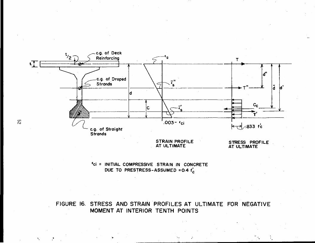
The computation of negative moment reinforcing for interior tenth

points is based on the assumptions listed in the previous section. The

computations for negative moment involve several additional considerations.

As shown in Fig. 16, the compressive strain in the concrete at failure is

the failure strain .003 in./in. minus the strain Eci produced by pre­

compression due to prestress. The strands are separated into straight

and drapped categories for computation of strand force. The ultimate

moment capacity of the section can be computed from

M = C d - T 1d 1 - T11 d 11

u c (73)

The va 1 ues of T 1 , d 1

, T11 and d 11 can be determined from the strain profile

in Fig. 17 and strand stress-strain characteristics, if the location of

the neutral axis c is known. The selection of the required area of deck

steel to resist a specified ultimate moment proceeds by establishing a

trial value of neutral axis location c which produces a net compressive

force Cc equal to the tensile forces in the strands (T 1 + T11). The

51

ti ~ / ~ . T

e.g. of. Draped Strands . , " ~ · -- ··· ·a ld'

'- I 1 I

d

_, Es

~ { ~ ~ .oo3- Ee• ~a33 fc

e.g. of Straight

\

Strands

STRAIN PROFILE STRESS PROFILE AT ULTIMATE AT ULTIMATE

tci = INITIAL COMPRESSIVE STRAIN IN CONCRETE DUE TO PRESTRESS-ASSUMED = 0.4 f~

FIGURE 16. STRESS AND STRAIN PROFILES AT ULTIMATE FOR NEGATIVE MOMENT AT INTERIOR TENTH POINTS

... ), ,'

U'1 w

t{· . .

• ~ ...

ts

d

,< .,

STRAIN PROFILE AT ULTIMATE

. "

T

d

Cc --

~.833f~

STRESS PROFILE AT ULTIMATE

FIGURE 17. STRESS AND STRAIN PROFILE AT ULTIMATE FOR NEGATIVE MOMENT AT END OF BEAM

moment capacity for this condition is computed and compared with that

required. If it exceeds the required moment (which can occur when the

e.g. of the draped strands is high), then no supplemental deck steel

is required to obtain the requisite capacity. If the strands alone

do not provide adequate tensile force, the location·of the neutral

axis c is incremented, the stress in the deck reinforcing is computed

from the known strain €s' and the area of steel necessary to satisfy

equilibrium, i.e.

T + T· + ru = cc (74)

is computed. Equation {73) is then used to compute capacity of the

section. If the capacity exceeds that required, the computations are

complete. If not, then c is incremented again and the process repeated.

The computation of negative moment reinforcing required at an end

of a beam differs from that just described in that the prestressing

strands are ineffective at this point. The pretension stress in the

strands is essentially zero at the end of the beam because of the

development length they require. Thus, they are ignored in the calcu­

lations. The strain profile must produce a compressive strain of .003

in./in. in the concrete at failure since there is no precompression from

prestress a.t this point. From Fig. 17, the ultimate moment capacity of

the section can be written as

M = C d u c

{75)

The area of reinforcing required is found by trial and error. A value

of the c is assumed, and the area of steel necessary to satisfy T = C c

54

-.

...

•'

. ""

is computed from the known steel strain Es· The capacity is then computed

from Eq. (75). If it is insufficient, c is increased and the process

repeated.

4.6 Computation of Positive Moment Reinforcement at Supports

Positive moments at interior supports will generally occur from live

loads in remote spans, and under certain conditions, from creep and

shrinkage restraint. Nonprestressed reinforcement is determined from

ultimate strength computations analagous to those for negative moment re­

inforcing at supports described in the previous section. The e.g. of the

reinforcing is assumed to be 2.5 in. from the bottom face of the beam. To

preclude fatigue failure of the bars, the stress produced by service live

loads is limited to 21 ksi.

4.7 Computation of Shear Reinforcing

The required area for stirrups are computed for three segments of

each span; left end to left quarter point, left quarter point to right

quarter point, and right quarter point to right end. The required areas

are computed from the worst condition within each segment. Stirrup

spacings are computed according to AASHTO (l) and ACI (I.) provis.ions.

The AASHTO provisions stipulate that

(76)

55

where

s = stirrup spacing,

A = area of stirrups required, v

Vu = largest (in absolute value) ultimate shear force existing in segment under consideration,

Vc = .06 f~b.jd, but not more than 180 b1 jd,

fsy= yield strength of reinforcing,

jd = 0.9 times the beam depth if the moment at the point under consideration is positive, and .875 times (beam depth - 1/2 slab thickness) if the moment is negative.

4> = 0.9

Vpr= vertical component of strand force (kips)

The required stirrup spacings can be obtained by solving Eq. (76).

The maximum spacing permitted is 12 inches (Section 1.6.14(0)).

Sections 11.1.2 and 11.6.1 of ACI gives the following expressions

for minimum required stirrup area (modified here to deduct the vertical

component of strand force from the shear carried by the section)

(77)

(78)

where

s = stirrup spacing,

bw = beam web width,

fy = yield strength of reinforcing,

vu = ultimate shear stress to be resisted, = VU/$ bwd

56

(

~-.

•

-----------------------------------------------------------------------------------

••

.,..

v = shear stress carried by the concrete section, given by c

v d vc = 1.6 ~ + 700 M u ; 2 {f{_ ~ vc < 5 ~

u

Vu' Mu = ultimate shear force and bending moment at the section,

(79}

d = effective depth. For positive moment it is the distance from the e.g. of the strands to the top of the beam or 0.8 times the beam depth, whichever is greater. For negative moment, it is the distance from the bottom of the beam to mid-depth of slab.

<P = 0.85

57

REFERENCES

1. Standard Specifications for Highway Bridges, American Association of State Highway Officials, 11th Edition, 1973.

2. Mattock, A. H., 11 Precast-Prestressed Concrete Bridges 5. Creep and Shrinkage Studies, 11 Journal of the Research and Development Laboratories, Portland Cement Association, Skokie, Illinois, Vol. 3, No. 2, May, 1 961 .

3. Ingram, L. L. and Furr, H. L., 11 Creep and Shrinkage of Concrete Based on Major Variables Encountered in the State of Texas, 11 Research Report 170-lF, Texas Transportation Institute, Texas A&M University, College Station, Texas.

4. Freyermuth, c. L. 11 Design of Continuous Highway Bridges with Precast, Prestressed Concrete Girders, 11 PC! Journal, April, 1969.

5. Hadley, G. F., Linear Programming, Addison-Wesley Publishing Co., Inc., Reading, Mass., 1962.

6. Bridge Design Manual, Texas Highway Department, Austin, Texas, January 15, 1965.

7. 11 Building Code Requirements for Reinforced Concrete (ACI 318-71), 11

American Concrete Institute, Detroit, Michigan, 1971.

8. Kaar, P. H., Kriz, L. B., and Hognestad, E., 11 Precast-Prestressed Concrete Bridges l. Pilot Tests of Continuous Beams, 11 Journa 1 of the Research and Development Laboratories, Portland Cement Assoc1at1on, Skokie, Illinois, Vol. 2, No.2, May 1960.

58

'( .-"

• ••

..,