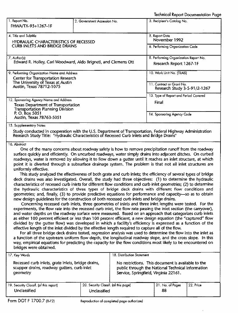
1 . Report No. 2. Government Accession No.

FHWA/TX-93+ 1267-1 F

4. Tirie and Subtirie

HYDRAULIC CHARACTERISTICS OF RECESSED CURB INLETS AND BRIDGE DRAINS

7. Author(s) Edward R. Holley, Carl Woodward, Aldo Brigneti, and Clemens Ott

9. Performing Organization Name and Address

Center for Transportation Research The University of Texas at Austin Austin, Texas 78712-1075

Technical Report Documentation Page 3. Recipient's Catalog No.

5. Report Date November 1992

6. Performing Organization Code

8. Performing Organization Report No.

Research Report 1267-1 F

1 0. Work Unit No. (TRAISJ

11. Contract or Grant No. Research Study 3-5-91 /2-1267

1-----------~~----------------l 13. Type of Report and Period Covered 12. Sponsoring Agency Name and Address Final

Texas Department of Transportation Transportation Planning Division P. 0. Box 5051 Austin, Texas 78763-5051

15. Supplementary Notes

14. Sponsoring Agency Code

Study conducted in cooperation with the U.S. Department of Transportation, Federal Highway Administration Research Study Title: "Hydraulic Characteristics of Recessed Curb Inlets and Bridge Drains"

16. Abstract

One of the many concerns about roadway safety is how to remove precipitation runoff from the roadway surface quickly and efficiently. On uncurbed roadways, water simply drains into adjacent ditches. On curbed roadways, water is removed by allowing it to flow down a gutter until it reaches an inlet structure, at which point it is diverted through a subsurface drainage system. The problem is that not all inlet structures are uniformly effective.

This study analyzed the effectiveness of both grate and curb inlets; the efficiency of several types of bridge deck drains was also investigated. Overall, the study had three objectives: (1) to determine the hydraulic characteristics of recessed curb inlets for different flow conditions and curb inlet geometries; (2) to determine the hydraulic characteristics of three types of bridge deck drains with different flow conditions and geometries; and, finally, (3) to provide predictive equations for performance and capacity-so as to obtain new design guidelines for the construction of both recessed curb inlets and bridge drains.

Concerning recessed curb inlets, three geometries of inlets and three inlet lengths were tested. For the experiments, the flow rate into the recessed curb inlet, the flow rate passing the inlet section (the carryover), and water depths on the roadway surface were measured. Based on an approach that categorizes curb inlets as either 1 00 percent efficient or less than 1 00 percent efficient, a new design equation (the "captured" flow divided by the gutter flow) was developed in which a facility's efficiency is expressed as a function of the effective length of the inlet divided by the effective length required to capture all of the flow.

For all three bridge deck drains tested, regression analysis was used to determine the flow into the inlet as a function of the upstream uniform flow depth, the longitudinal roadway slope, and the cross slope. In this way, empirical equations for predicting the capacity for the flow conditions most likely to be encountered on bridges were obtained.

17. Key Words

Recessed curb inlets, grate inlets, bridge drains, scupper drains, roadway gutters, curb inlet geometry

18. Distribution Statement

No restrictions. This document is available to the public through the National Technical Information Service, Springfield, Virginia 22161.

19. Security Clossif. (of this report}

Unclassified

20. Security Classif. (of this page)

Unclassified

21 . No. of Pages

88 22. Price

Form DOT F 1700.7 (8-72) Reproduction of completed page authorized

HYDRAULIC CHARACTERISTICS OF RECESSED CURB INLETS AND BRIDGE DRAINS

by

Edward R. Holley Carl Woodward Aldo Brigneti Clemens Ott

Research Report 1267-lF

Hydraulic Characteristics of Recessed Curb Inlets and Bridge Drains Research Project 3-5-91/1267

conducted for the

Texas Department of Transportation

in cooperation with the

U.S. Department of Transportation Federal Highway Administration

by the

CENTER FOR TRANSPORTATION RESEARCH

Bureau of Engineering Research THE UNIVERSITY OF TEXAS AT AUSTIN

November 1992

ii

DISCLAIMERS

The contents of this report reflect the views of the authors, who are responsible for the facts and the accuracy of the data presented herein. The contents do not necessarily reflect the official views or policies of the Federal Highway Administration or the Texas Department of Transportation. This re­port does not constitute a standard, specification, or regulation.

There was no invention or discovery conceived or first actually reduced to practice in the course of or under this contract, including art, method, process, machine, manufacture, design or composition of matter, or any new and useful improvement thereof, or any variety of plant which is or may be patentable under the patent laws of the United States of America or any foreign country.

NOT INTENDED FOR CONSTRUCTION, PERMIT, OR BIDDING PURPOSES

Edward R. Holley, P.E. (Texas No. 51638) Study Supervisor

iii

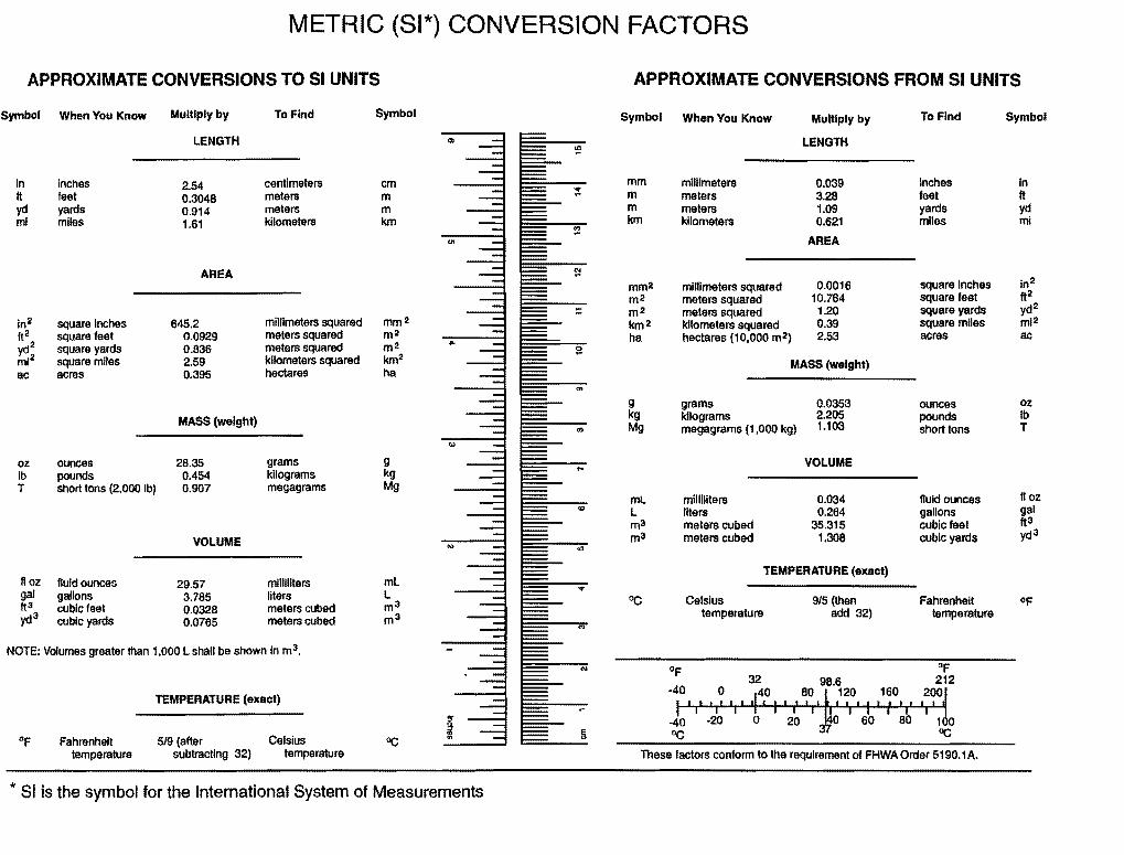
METRIC (SI*) CONVERSION FACTORS

APPROXIMATE CONVERSIONS TO Sl UNITS

Symbol When You Know

in inches ft feet yd yards mi miles

oz lb T

square inches square feet square yards square miles acres

ounces pounds short tons (2,000 lb)

II oz lluld ounces gal gallons ft 3 cubic feet yd3 cubic yards

Multiply by

LENGTH

2.54 0.3048 0.914 1.61

AREA

645.2 0.0929 0.836 2.59 0.395

MASS (weight)

28.35 0.454 0.907

VOLUME

29.57 3.785 0.0328 0.0765

To Find

centimeters meters meters kilometers

millimeters squared meters squared meters squared kilometers squared hectares

grams kilograms mega grams

milliliters liters meters cubed meters cubed

NOTE: Volumes greater than 1,000 L shall be shown In m3 .

TEMPERATURE (exact)

Fahrenheit 5/9 {after Celsius temperature subtracting 32) temperature

Symbol

em m m km

mm2 m2 m2 km2 ha

g kg Mg

* 81 is the symbol for the International System of Measurements

APPROXIMATE CONVERSIONS FROM Sl UNITS

Symbol When You Know

mm millimeters m meters m meters km kilometers

mm2 m2 m2 km2 ha

millimeters squared meters squared meters squared kilometers squared hectares {10,000 m2)

Multiply by

LENGTH

0.039 3.28 1.09 0.621

AREA

0.0016 10.764 1.20 0.39 2.53

MASS (weight)

g kg Mg

ml L m3 m3

grams kilograms megagrams {1,000kg)

milliliters liters meters cubed meters cubed

0.0353 2.205 1.103

VOLUME

0.034 0.264

35.315 1.308

TEMPERATURE (exact)

Celsius temperature

32 -40 0 40 I I I I I I I ·I· I I I I

-40 ·20 0 oc

9/5 {then add 32)

To Find

Inches feet yards miles

square Inches square feet square yards square miles acres

ounces pounds short tons

fluid ounces gallons cubic feet cubic yards

Fahrenheit temperature

I 100 oc

These factors conform to the requirement of FHWA Order 5190.1 A.

Symbol

in ft yd mi

oz lb T

lloz gal ft3 yd3

TABLE OF CONTENTS

DISCLAIMERS ...................................................................... 0 •••••••••••••••••••••••••••••••••••••••••••••••• iii

METRICATION ......................................................................................................................... iv

SUMMARY ............................................................................................................ .................... vii

CHAPTER 1. INTRODUCTION 1.1 BACKGROUND ............................................................................................................... 1 1.2 OBJECTIVES .................................................................................................................... 1 1.3 APPROACH ..................................................................................................................... 1 1. 4 A CKN 0 WLEDG EMENTS ................................................................................................ 2

PART I. RECESSED CURB INLETS

CHAPTER 2. LITERATURE REVIEW 2.1 FLOW OVER A BROAD-CRESTED WEIR (IZZARD, 1950) ..................................... .4 2.2 FLOW OVER A FREE DROP (LI, 1954) ..................................................................... 5 2.3 COMPARISONS OF THE TWO METHODS ................................................................. 6 2.4 OTHER INVESTIGATIONS ............................................................................................ 7 2.5 MODIFIED MANNING'S EQUATION ........................................................................... 9

CHAPTER 3. THE PHYSICAL MODEL 3.1 MODEL LENGTH SCALE ............................................................................................ 11 3.2 MODEL CONSTRUCTION ........................................................................................... 11 3.3 MODEL LAYOUT ......................................................................................................... 12 3.4 RECESSED CURB INLET GEOMETRY ........................................................................ 13 3.5 ROADWAY ROUGHNESS ............................................................................................ 13 3.6 MEASUREMENTS .......................................................................................................... 14

3.6.1 Venturi Meter for the North Pipe ............................................................................ 14 3.6.2 Flow Sensor for the South Pipe ............................................................................... 15 3.6.3 V-Notch Weir for the Carryover .............................................................................. 16 3.6.4 V-Notch Weir for Total Discharge .......................................................................... 16 3.6.5 Water Surface Elevation Measurement .................................................................... 17

3.7 DATA ANALYSIS .......................................................................................................... 18

CHAPTER 4. EXPERIMENTAL RESULTS 4.1 EXPERIMENTAL LABORATORY PROCEDURES ........................................................ 19

4.1.1 Reverse Curve Transition ......................................................................................... 19 4.1.2 Linear Transition ..................................................................................................... 20 4.1.3 20% Recessed Slope ................................................................................................. 20

4.2 LABORATORY RESULTS FOR REVERSE CURVE TRANSITIONS ............................ 20 4.2.1 Inlet Efficiency= 100% ........................................................................................... 20 4.2.2 Results for Inlet Efficiency < 100% ........................................................................ 22

4.2.2.1 Analysis in Terms of Efficiency ....................................................................... 22 4.2.2.2 Analysis of Residuals ....................................................................................... 23 4.2.2.3 Effects of Inlet Length and Froude Number .................................................... 23 4.2.2.4 Comparison to Flush Inlets ............................................................................. 25

4.3 LABORATORY RESULTS FOR LINEAR TRANSITIONS ............................................ 26 4.3.1 Inlet Efficiency = 100% ........................................................................................... 26 4.3.2- Inlet Efficiency < 100% ........................................................................................... 26

4.4 LABORATORY RESULTS FOR 20% RECESSED SLOPE ............................................ 27 4.5 FIELD- TESTS ................................................................................................................ 28

4.5.1 Procedures ....................................................................................... ~ ........................ 28 4.5.2 Results ...................................................................................................................... 29

CHAPTER S. CONCLUSIONS FOR RECESSED CURB INLETS ................................. 31

PART II. BRIDGE DECK DRAINS

CHAPTER 6. INTRODUCTION ......................................................................................... 33

CHAPTER 7. EXPERIMENTS AND RESULTS 7.1 THE PHYSICAL MODEL ............................................................................................. 35 7.2 MEASUREMENTS .......................................................................................................... 35 7.3 DRAIN 1 (SCUPPER DRAIN) ...................................................................................... 36

7.3.1 Geometry and Description ....................................................................................... 36 7.3.2 Procedures ................................................................................................................. 36 7.3.3 Results ...................................................................................................................... 36 7.3.4 Limits of Applicability ............................................................................................. 38

7.4 DRAIN 2 ....................................................................................................................... 38 7.4.1 Geometry and Description ....................................................................................... 38 7.4.2 Procedures ................................................................................................................. 39 7.4.3 Results ...................................................................................................................... 41

7.4.3.1 Effects of Piping System ................................................................................... 41 7.4.3.2 Results for Low Flow Conditions ..................................................................... 42

7.4.4 Limits of Applicability ............................................................................................. 44 7.4.5 Comparison of Results for Drain 2 with HEC~12 ................................................. .44

7.5 DRAIN 3 ....................................................................................................................... 44 7.5.1 Geometry and Description ....................................................................................... 44 7.5.2 Procedures ................................................................................................................. 45 7.5.3 Results ...................................................................................................................... 45 7.5.4 Limits of Applicability ............................................................................................. 46 7.5.5 Comparison of Results for Drain 3 with HEC~12 ................................................. .46

CHAPTER 8. CONCLUSIONS FOR BRIDGE DECK DRAINS ..................................... 51

REFERENCES ........................................................................................................................... 53

APPENDIX A. DATA FOR RECESSED CURB INLETS ................................................ 55

APPENDIX B. DATA FOR BRIDGE DECK DRAINS .................................................... 65

APPENDIX C. PHOTOGRAPHS ........................................................................................ 73

vi

SUMMARY

The hydraulic characteristics of flow into roadway drainage facilities and the flow capacity of these facilities are important considerations from the standpoints of both safety and possible nuisance. Pre­vious studies have been done on curb inlets and bridge deck drains, but the designs of these facilities are sometimes changed for various reasons. Changes in the geometry of drainage facilities also affect the hydraulics and the flow capacity. These types of changes have meant that some drains have been installed after being designed by inference from other similar facilities since design information on the particular geometries being used was not available. This was the case for the recessed curb inlets and the three types of bridge deck drains which were studied in this project.

In order to obtain design information for these inlets and drains, a large hydraulic model was de­signed and constructed. The model was 64 feet long and 10.5 feet wide to represent one lane of a roadway at three-quarters scale. It was constructed so that both the cross slope and the longitudinal slope could be easily changed. The roadway surface had a uniform cross slope, not a compound slope. There was no depression in front of the curb line.

A literature review was conducted, primarily to determine the source of some of the design infor­mation which is normally used for curb inlets. This review located two different analyses which ap­pear to be the background for dividing the flow into curb inlets into separate categories for 100% efficiency and less than 100% efficiency. Although the general forms of the two equations in the lit­erature for 100% efficiency were the same, the numerical coefficients were different. For less than 100% efficiency, the basic forms of the equations were significantly different. Each of the authors compared the equations to experimental data, apparently indicating that the details of roadway geometry can have a significant influence on the capacity of inlets.

For the recessed curb inlets, three geometries of inlets and three inlet lengths were tested. The first geometry had reverse curve transitions 10 feet long at both ends of the inlet opening, which was re­cessed 1.5 feet from the curb line. (All dimensions are prototype sizes unless stated differently.) Inlet lengths of 15, 10, and 5 feet were tested. For 100% efficiency, it was possible to obtain basically the same type of design equation as is used for flush inlets by defining an effective length of the inlet to be used in place of the actual length of a flush inlet. For the reverse curve transitions, the effective length at 100% efficiency was 2 feet shorter than the total length of the curb opening. For less than 100% effi­ciency, the downstream transition section loses effectiveness for capturing flow. Even after water crosses the curb line and enters the region of the downstream transition, the momentum of the flow can cause it to flow back up the slope behind the curb line and back into the street. Thus, for less than 100% efficiency, a recessed inlet with the same actual opening length as a flush inlet may be only slightly more effective than a flush inlet with the same opening length. A new design equation was developed for the efficiency of the inlet (the flow captured divided by the gutter flow) as a function of the effective length of the inlet divided by the effective length required to capture all of the flow.

After completing the analysis of the tests with reverse curve transitions, a smaller number of tests were done for linear transition sections and for the slope from the gutter line to the inlet opening reduced from 30% to 20%. Neither of these changes had a significant effect on the results, other than that the effective length for the linear transition sections included the entire 10 feet of the downstream transition section, rather than only 8 feet as for the reverse curve transitions. Thus, the linear transi­tions are slightly more efficient than the reverse curves.

The three types of bridge deck drains were a 4-inch-by-6-inch rectangular scupper and two types of grated inlets. The scupper and the smaller grated inlet were tested at full scale, while the larger grated inlet was tested at three-quarters scale. All of the inlets were constructed of plexiglass so that the flow in the inlet boxes and in the subsequent piping could be seen. For each of the drains, the flow regimes fell into either of two categories. For the lower gutter depth and flows, the flow into the drain was ap-

vii

parently controlled by weir flow over the lip of the inlets or orifice control as the water flowed from the inlet box into the drain pipe. (For the scupper, the only possibility was weir control since there was no subsequent piping.) For higher flows for the two grated inlets, there were back-pressure effects from the drain piping. One of the grated inlets is normally followed by 6-inch drain piping. For this inlet, several different configurations of piping were first tested to determine the effects on the flow into the inlet. It was determined that the most critical situation existed when the first elbow in the piping sys­tem was closest to the bottom of the inlet box. Thus, this configuration was used for the remainder of the tests. The tests revealed that the most likely range of inlet flows for these bridge drains fell into the low flow regime. Thus, attention was concentrated on these conditions for developing design informa­tion. For each of the drains, regression analysis was used to determine the flow into the inlet as a func­tion of the upstream uniform flow depth, the longitudinal roadway slope, and the cross slope.

viii

CHAPTER 1.

1.1 BACKGROUND

One of the many concerns about roadway safety is how to remove precipitation runoff from the roadway surface and adjacent areas quickly and efficiently. On uncurbed roadways, water simply drains into adjacent ditches. With curbed roadways, the basic principle of removal is to allow the water to flow down the gutter until it reaches an inlet structure. After the wa­ter enters the inlet, it flows away from the road­way through a subsurface drainage system. Simi­larly, runoff from bridge decks is captured by bridge deck drains. Depending on the type of bridge deck drain, the water may then fall freely through the air or it may flow downward through a piping system.

Inability of inlets and drains to adequately in­tercept the runoff results in water standing on the roadway and possibly on adjacent property. Stand­ing water threatens traffic safety by causing hydro­planing of vehicles, deterioration of the pavement due to the seepage of water, and accumulation of sediments and debris in low areas.

Several types of inlet structures are used for roadways. Two of the primary types are grate in­lets and curb inlets. A grate inlet uses metal bars placed in the roadway surface with the bars par­allel and/or perpendicular to the flow of water. Flush inlets are simply vertical openings in the curb face and may or may not have a depression in the roadway adjacent to the inlet. According to Wasley (1960), grate inlets allow more flow to enter per given length than flush curb inlets. One drawback of grate inlets is their high probability of clogging since the opening between the bars is smaller than the opening for a curb inlet. Another potential problem is interference with traffic. Clogging is not often a problem with curb inlets. Unlike the grate inlet, the curb inlet does not interfere with traffic. A third type of inlet is a combination inlet, which uses a curb opening inlet and a grate inlet. One of the purposes of combining the two types of inlets is to achieve

INTRODUCTION

1

good efficiency while minimizing the potential for clogging.

Similarly, several types of bridge deck drains ex­ist. These drains may be either open scupper drains with subsequent free fall of the captured runoff or grated drains in the bridge decks with a variety of geometries of the grates, of the boxes beneath the grates, and of the subsequent drain pipes.

1.2 OBJECTIVES

The primary objectives of this research were to

1. determine hydraulic characteristics of re­cessed curb inlets for different flow condi­tions and curb inlet geometries;

2. determine hydraulic characteristics of three types of bridge deck drains with different flow conditions and geometries; and

3. develop design information related to objec­tives 1 and 2.

1.3 APPROACH

The primary variables which influence the amount of flow captured by inlets and drains are longitudinal gutter slope, transverse pavement slope and geometry, flow rate in the gutter, Manning's roughness, flow regime (i.e., whether the flow is subcritical or supercritical), and inlet or drain size and geometry. Obtaining mathemati­cal solutions for the amount of flow captured is a very complex problem. In fact, the computa­tional approach is so complex that it would re­quire verification against experimental results before complete confidence could be placed in the results of the computations. Thus, the primary approach for accomplishing the project objectives (Section 1.2) was to construct a large, versatile physical model of a roadway and to conduct a large number of experiments to cover the ex­pected flow conditions and geometries of recessed curb inlets and bridge deck drains. Field testing of recessed curb inlets was also done to verify the

results of the laboratory tests on these inlets. Apparently, no hydraulic data previously existed for recessed curb inlets, which were being de­signed by inference from other types of inlets. The three bridge deck drains were also being de­signed without any hydraulic data on these spe­cific geometries of drains. In addition, for the two drains with piping systems below them, attention was given to the effects of the piping on the drain capacity and hydraulic behavior.

Following Chapter 1, the remainder of the re­port is divided into two parts. Part I (Chapters 2-5) is for recessed curb inlets, and Part II (Chap­ters 6-8) is for bridge deck drains. Part I includes a description of the model facility. The data for Parts I and II are in Appendices A and B, respec­tively. Appendix C contains photographs. Some of the equations in this report are given in dimen­sionally consistent equations; such equations may be used with any set of consistent units. When specific units are needed for the equations which are not dimensionally consistent, traditional En­glish units are used throughout.

1.4 ACKNOWLEDGEMENTS

This research was funded by the Texas Depart­ment of Transportation (TxDOT) through the

2

Center for Transportation Research (CTR) at The University of Texas at Austin. The project num­ber was 3-5-91/2-1267, entitled "Hydraulic Char­acteristics of Recessed Curb Inlets and Bridge Deck Drains." The research was conducted at the Center for Research in Water Resources. The graduate students (Carl Woodward, Aldo Brigneti, Clemens Ott, and Clint Willson) actually carried out the primary parts of the research. Various ones of them designed the physical model, su­pervised and assisted with the model construc­tion, conducted the tests, analyzed the data, and wrote the first draft of different parts of this re­port. M. D. Englehardt and other personnel as­sociated with the Ferguson Structural Engineer­ing Laboratory of The University of Texas at Austin provided significant assistance with struc­tural aspects of designing and constructing the roadway model. The project was supervised pri­marily by E. R. Holley and also by G. H. Ward. The supervisors were intimately involved in all aspects of the planning and execution of the project. E. R. Holley prepared the final draft of this report. Peter Smith of the Division of Bridges and Structures, TxDOT, was the Technical Panel Chair. He was extremely helpful in all phases of the research from its conception through its ex­ecution to the writing of this report.

PART I. RECESSED CURB INLETS

CHAPTER 2. LITERATURE REVIEW

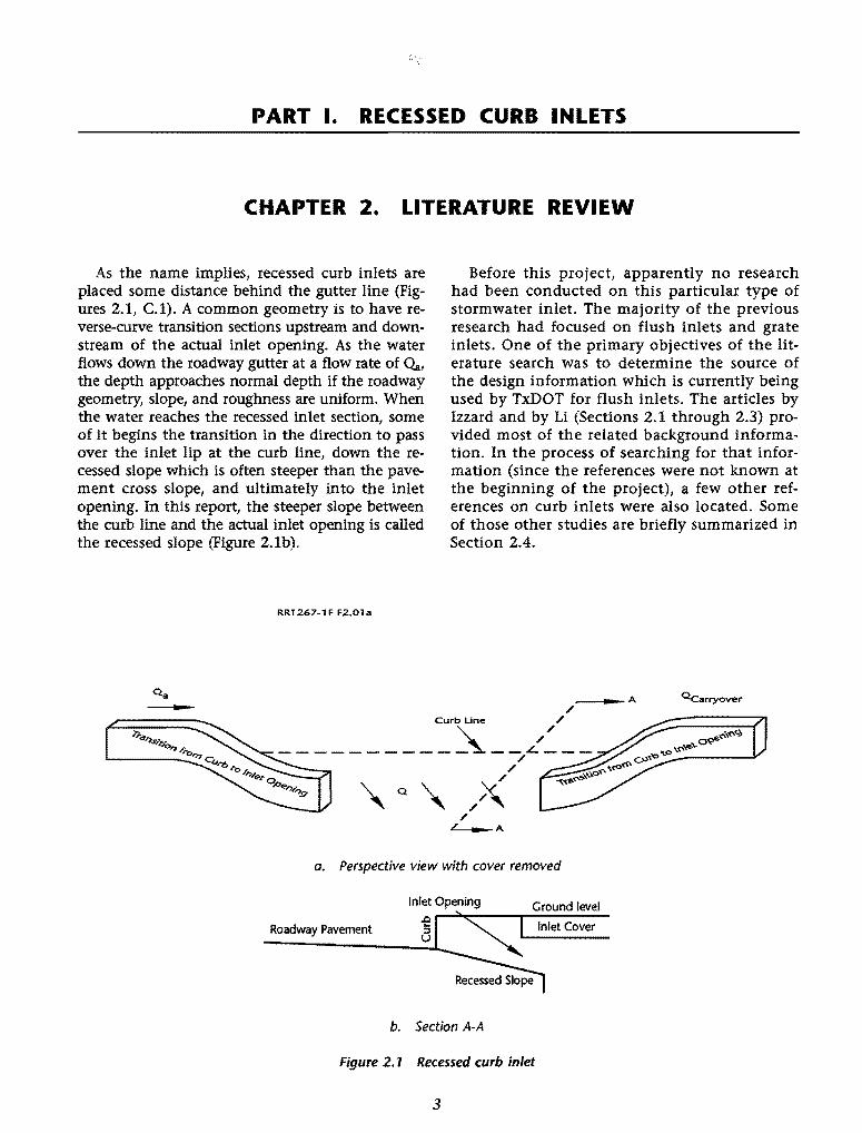
As the name implies, recessed curb inlets are placed some distance behind the gutter line (Fig­ures 2.1, C.1). A common geometry is to have re­verse-curve transition sections upstream and down­stream of the actual inlet opening. As the water flows down the roadway gutter at a flow rate of Oa, the depth approaches normal depth if the roadway geometry, slope, and roughness are uniform. When the water reaches the recessed inlet section, some of it begins the transition in the direction to pass over the inlet lip at the curb line, down the re­cessed slope which is often steeper than the pave­ment cross slope, and ultimately into the inlet opening. In this report, the steeper slope between the curb line and the actual inlet opening is called the recessed slope (Figure 2.1b).

RR1267-1 F F2.01a

..

Before this project, apparently no research had been conducted on this particular type of stormwater inlet. The majority of the previous research had focused on flush inlets and grate inlets. One of the primary objectives of the lit­erature search was to determine the source of the design information which is currently being used by TxDOT for flush inlets. The articles by Izzard and by Li (Sections 2.1 through 2.3) pro­vided most of the related background informa­tion. In the process of searching for that infor­mation (since the references were not known at the beginning of the project), a few other ref­erences on curb inlets were also located. Some of those other studies are briefly summarized in Section 2.4.

- A ~arryove~

/ Curb Line /

----------~--L~--/

/

"' Q "' /)\ / ~A

/

a. Perspective view with cover removed

Roadway Pavement

Inlet Opening .!:2 5 u

b. Section A-A

Ground level

Inlet Cover

Figure 2.1 Recessed curb inlet

3

2.1 FLOW OVER A BROAD-CRESTED WEIR (IZZARD, 1950)

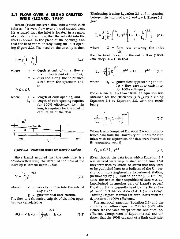
Izzard (1950) analyzed flow into a flush curb inlet as if it were flow over a broad-crested weir. He assumed that the inlet is located in a region of constant gutter slope, that the velocity into the inlet is normal to the plane of the opening, and that the head varies linearly along the inlet open­ing (Figure 2.2). The head on the inlet lip is then

where

where

(2.1)

y = depth at curb of gutter flow at the upstream end of the inlet,

x = distance along the inlet mea­sured from the upstream end, so

L = length of curb opening, and Lr = length of curb opening required

for 100% efficiency, i.e., the length required for the inlet to capture all of the flow.

Figure 2.2 Definition sketch for Izzard's analysis

Since Izzard assumed that the curb inlet is a broad-crested weir, the depth of the flow at the inlet lip is critical depth. Thus

[2 ]0.5

V= 3

gh (2.2)

where V = velocity of flow into the inlet at any x and

g gravitational acceleration. The flow rate through a strip dx of the inlet open­ing was calculated as

[ 2 r·5

dQ = v h d.x = 3 gh h d.x (2.3)

4

Eliminating h using Equation 2.1 and integrating between the limits of x = 0 and x = L (Figure 2.2) gave

2 [2 ]0.5 [ ( L J2.5] Q = S 3 g Lr yL5 1- 1- Lr (2.4)

where Q = flow rate entering the inlet (cfs).

For the inlet to capture the entire flow (100% efficiency), L = Lr so that

2[2 r·5

Qa = S 3g Lr y1.5 = 1.85 Lr y1.5 (2.5)

where (4 = gutter flow approaching the in-let = flow rate into curb inlet for 100% efficiency.

For efficiencies less than 100%, an equation was obtained for the efficiency (Q/Oa) by dividing Equation 2.4 by Equation 2.5, with the result being

(2.6)

When Izzard compared Equation 2.6 with unpub­lished data from the University of Illinois for curb inlets with no depression, the data were found to fit reasonably well if

(2.7)

(Even though the data from which Equation 2.7 was derived were unpublished at the time that they were used by Izzard, he stated that they were to be published later in a bulletin of the Univer­sity of Illinois Engineering Experiment Station, presumably by J. ]. Doland and/or J. C. Guillou, since the use of their unpublished data was ac­knowledged in another part of Izzard's paper.) Equation 2.7 is presently used by the Texas De­partment of Transportation (TxDOT) in its Design Training Program manual for curb inlets with no depression at 100% efficiency.

The analytical equation (Equation 2.5) and the empirical equation (Equation 2.7) for 100% effi­ciency are the same except for the numerical co­efficient. Comparison of Equations 2.5 and 2.7 shows that the 100% capacity of a flush curb inlet

is actually 0.7/1.85, or about 40% of the flow which would be predicted by the assumptions made by Izzard. One of the primary reasons for the smaller numerical coefficient in Equation 2. 7 is that Izzard effectively assumed that only gravity influences the motion of the water at the lip of the inlet. Actually, while gravity is tending to cause the water to flow into the inlet, the momentum of the gutter flow parallel to the curb is tending to cause the water to flow past the inlet opening.

For depressed curb inlets, Izzard presented a modification of Equation 2. 7 for 100% effi­ciency, namely

(2.8)

where a = depression (ft) of the inlet lip below the normal gutter flow line at the face of curb.

Equation 2.8 overpredicted the flow captured by inlets tested at North Carolina State College (Conner, 1945) with a 3-inch depression and underpredicted data from inlets tested by the Corps of Engineers (1949) with a 2-inch depression.

Izzard grouped these two data sets with the unpublished data from the University of Illinois with no depression but with a composite cross slope, i.e., a steeper cross slope in the gutter than in the remainder of the roadway (as shown later in Figure 2.7), and compared Equation 2.8 with all of the data. He recognized that there was a signifi­cant amount of scatter but concluded that the agreement between Equation 2.8 and the data was adequate for design purposes. Part of the scatter of the data compared to Equation 2.8, and part of the differences between the three data sets may be due to the fact that the geometry of the depression was different in the three sets of experiments.

TxDOT's Design Training Program manual pres­ently uses an equation similar to Equation 2.8 for curb inlets to capture the total approach gutter flow for undepressed and depressed curb inlets. For less than 100% efficiency, TxDOT's Design Training Program manual uses Equation 2.6 for undepressed curb inlets.

2.2 FLOW OVER A FREE DROP (LI, 1954)

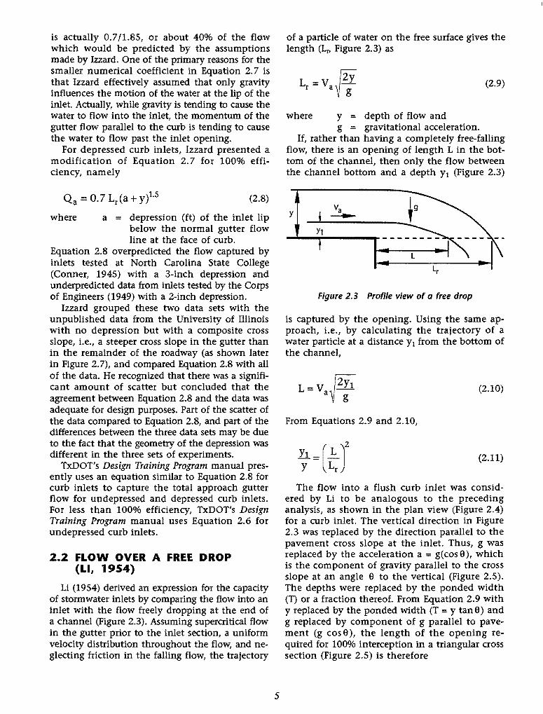
Li (1954) derived an expression for the capacity of stormwater inlets by comparing the flow into an inlet with the flow freely dropping at the end of a channel (Figure 2.3). Assuming supercritical flow in the gutter prior to the inlet section, a uniform velocity distribution throughout the flow, and ne­glecting friction in the falling flow, the trajectory

5

of a particle of water on the free surface gives the length (Lr, Figure 2.3) as

(2.9)

where y = depth of flow and g = gravitational acceleration.

If, rather than having a completely free-falling flow, there is an opening of length L in the bot­tom of the channel, then only the flow between the channel bottom and a depth y1 (Figure 2.3)

__..Y ~y ........ ;,~----_v_a ==~-:..---k--

Figure 2.3 Profile view of a free drop

is captured by the opening. Using the same ap­proach, i.e., by calculating the trajectory of a water particle at a distance y 1 from the bottom of the channel,

(2.10)

From Equations 2.9 and 2.10,

y =(tJ (2.11)

The flow into a flush curb inlet was consid­ered by Li to be analogous to the preceding analysis, as shown in the plan view (Figure 2.4) for a curb inlet. The vertical direction in Figure 2.3 was replaced by the direction parallel to the pavement cross slope at the inlet. Thus, g was replaced by the acceleration a= g(cos9), which is the component of gravity parallel to the cross slope at an angle 9 to the vertical (Figure 2.5). The depths were replaced by the ponded width (T) or a fraction thereof. From Equation 2.9 with y replaced by the ponded width (T = y tan9) and g replaced by component of g parallel to pave­ment (g cosO), the length of the opening re­quired for 100% interception in a triangular cross section (Figure 2.5) is therefore

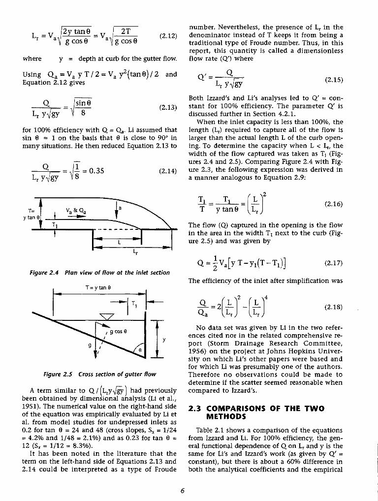
L -v f2ytan9 -v ~ r- aV g COS 9 - a~gcose (2.12)

where y = depth at curb for the gutter flow.

Using Qa = Va y T /2 = Va yZ(tan9) /2 and Equation 2.12 gives

number. Nevertheless, the presence of Lr in the denominator instead of T keeps it from being a traditional type of Froude number. Thus, in this report, this quantity is called a dimensionless flow rate (Q') where

(2.15)

Both Izzard's and Li's analyses led to Q' = con-(2.13) stant for 100% efficiency. The parameter Q' is

discussed further in Section 4.2.1.

for 100% efficiency with Q = Oa. Li assumed that sin e = 1 on the basis that e is close to 90° in many situations. He then reduced Equation 2.13 to

Jgy = /l = 0.35 LrY gy Vs

T= ytan a

(2.14)

Figure 2.4 Plan view of flow at the inlet section

T=ytane

Figure 2.5 Cross section of gutter flow

A term similar to Q I ( LrY -[gY) had previously been obtained by dimensional analysis (Li et al., 1951). The numerical value on the right-hand side of the equation was empirically evaluated by Li et al. from model studies for undepressed inlets as 0.2 for tan e = 24 and 48 (cross slopes, Sx = 1/24 = 4.2% and 1/48 ;::: 2.1 %) and as 0.23 for tan e = 12 (Sx = 1/12 = 8.3%).

It has been noted in the literature that the term on the left-hand side of Equations 2.13 and 2.14 could be interpreted as a type of Froude

6

When the inlet capacity is less than 100%, the length (Lr) required to capture all of the flow is larger than the actual length L of the curb open­ing. To determine the capacity when L < 4, the width of the flow captured was taken as T1 (Fig­ures 2.4 and 2.5). Comparing Figure 2.4 with Fig­ure 2.3, the following expression was derived in a manner analogous to Equation 2.9:

(2.16)

The flow (Q) captured in the opening is the flow in the area in the width T 1 next to the curb (Fig­ure 2.5) and was given by

(2.17)

The efficiency of the inlet after simplification was

(2.18)

No data set was given by Li in the two refer­ences cited nor in the related comprehensive re­port (Storm Drainage Research Committee, 1956) on the project at Johns Hopkins Univer­sity on which Li's other papers were based and for which Li was presumably one of the authors. Therefore no observations could be made to determine if the scatter seemed reasonable when compared to Izzard's.

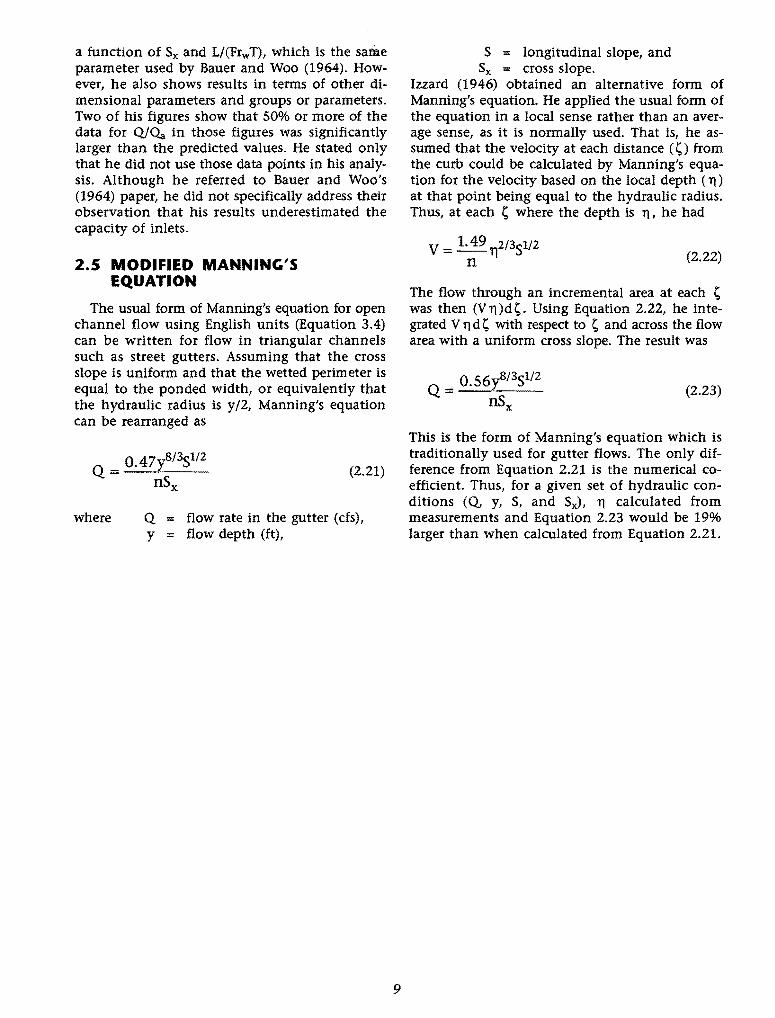
2.3 COMPARISONS OF THE TWO METHODS

Table 2.1 shows a comparison of the equations from Izzard and Li. For 100% efficiency, the gen­eral functional dependence of Q on Lr and y is the same for Li's and Izzard's work (as given by Q' = constant), but there is about a 60% difference in both the analytical coefficients and the empirical

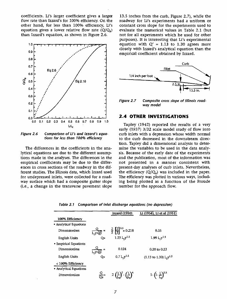
coefficients. Li's larger coefficient gives a larger flow rate than Izzard's for 100% efficiency. On the other hand, for less than 100% efficiency, Li's equation gives a lower relative flow rate (Q/Oa) than Izzard's equation, as shown in Figure 2.6.

00$

0

1.0

0.9

0.8

0.7

0.6

0.5

0.4

0.3

0.2

0.1

0.0 t.....lo:::;:;J.._._.J.......I-.L.....I.....I......JL..-l..-J...-'-1..-L-'--'--"--'--'--'

o.o 0.1 0.2 0.3 0.4 0.5 0.6 0.7 0.8 0.9 1.0

LILr

Figure 2.6 Comparison of Li's and Izzard's equa­tions for less than 7 00% efficiency

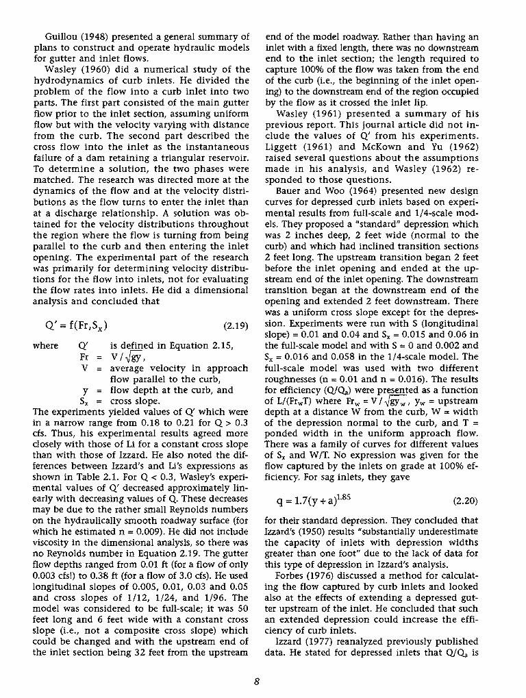
The differences in the coefficients in the ana­lytical equations are due to the different assump­tions made in the analyses. The differences in the empirical coefficients may be due to the differ­ences in cross sections of the roadway in the dif­ferent studies. The Illinois data, which Izzard used for undepressed inlets, were collected for a road­way surface which had a composite gutter slope (i.e., a change in the transverse pavement slope

13.5 inches from the curb, Figure 2.7), while the roadway for Li's experiments had a uniform or constant cross slope for the experiments used to evaluate the numerical values in Table 2.1 (but not for all experiments which he used for other purposes). It is interesting that Li's experimental equation with Q' = 1.13 to 1.30 agrees more closely with Izzard's analytical equation than the empirical coefficient obtained by Izzard.

Curb

Fillet

1/4 inch per foot

Figure 2.7 Composite cross slope of Illinois road­way model

2.4 OTHER INVESTIGATIONS

Tapley (1942) reported the results of a very early (1937) 3/32 scale model study of flow into curb inlets with a depression whose width normal to the curb decreased in the downstream direc­tion. Tapley did a dimensional analysis to deter­mine the variables to be used in the data analy­sis. Because of the early date of the experiments and the publication, most of the information was not presented in a manner consistent with present-day analyses of curb inlets. Nevertheless, the efficiency (Q/Oa) was included in the paper. The efficiency was plotted in various ways, includ­ing being plotted as a function of the Froude number for the approach flow.

Table 2. 7 Comparison of inlet discharge equations (no depression)

Izzard (1950) Li (1954), Li et al (1951)

100% Efficiency

• Analytical Equations

Dimensionless _g_= 2 ~~0.5 0.35 Lry{gy ! "! =0.218

English Units Q= 1.23 l.rYI.s 1.99 l.rYI.S

• Empirical Equations

Dimensionless _g_= 0.124 0.20to0.23 Lry{if

English Units Q= 0.7 I,.yl.S (1.13 to 1.30) I,.y1.5

< 100% Efficiency

• Analytical Equations

Dimensionless _g_= 2 (f)2- (t)4 ~ fJ~s Qa

1- 1--

7

Guillou (1948) presented a general summary of plans to construct and operate hydraulic models for gutter and inlet flows.

Wasley (1960) did a numerical study of the hydrodynamics of curb inlets. He divided the problem of the flow into a curb inlet into two parts. The first part consisted of the main gutter flow prior to the inlet section, assuming uniform flow but with the velocity varying with distance from the curb. The second part described the cross flow into the inlet as the instantaneous failure of a dam retaining a triangular reservoir. To determine a solution, the two phases were matched. The research was directed more at the dynamics of the flow and at the velocity distri­butions as the flow turns to enter the inlet than at a discharge relationship. A solution was ob­tained for the velocity distributions throughout the region where the flow is turning from being parallel to the curb and then entering the inlet opening. The experimental part of the research was primarily for determining velocity distribu­tions for the flow into inlets, not for evaluating the flow rates into inlets. He did a dimensional analysis and concluded that

Q' = f(Fr,Sx) (2.19)

where Q' is defined in Equation 2.15, Fr = V/~, V = average velocity in approach

flow parallel to the curb, y = flow depth at the curb, and

Sx = cross slope. The experiments yielded values of Q' which were in a narrow range from 0.18 to 0.21 for Q > 0.3 cfs. Thus, his experimental results agreed more closely with those of Li for a constant cross slope than with those of Izzard. He also noted the dif­ferences between Izzard's and Li's expressions as shown in Table 2.1. For Q < 0.3, Wasley's experi­mental values of Q' decreased approximately lin­early with decreasing values of Q. These decreases may be due to the rather small Reynolds numbers on the hydraulically smooth roadway surface (for which he estimated n = 0.009). He did not include viscosity in the dimensional analysis, so there was no Reynolds number in Equation 2.19. The gutter flow depths ranged from 0.01 ft (for a flow of only 0.003 cfs!) to 0.38 ft (for a flow of 3.0 cfs). He used longitudinal slopes of 0.005, 0.01, 0.03 and 0.05 and cross slopes of 1/12, 1/24, and 1/96. The model was considered to be full-scale; it was 50 feet long and 6 feet wide with a constant cross slope (i.e., not a composite cross slope) which could be changed and with the upstream end of the inlet section being 32 feet from the upstream

8

end of the model roadway. Rather than having an inlet with a fixed length, there was no downstream end to the inlet section; the length required to capture 100% of the flow was taken from the end of the curb (i.e., the beginning of the inlet open­ing) to the downstream end of the region occupied by the flow as it crossed the inlet lip.

Wasley (1961) presented a summary of his previous report. This journal article did not in­clude the values of Q' from his experiments. Liggett (1961) and McKown and Yu (1962) raised several questions about the assumptions made in his analysis, and Wasley (1962) re­sponded to those questions.

Bauer and Woo (1964) presented new design curves for depressed curb inlets based on experi­mental results from full-scale and 1/4-scale mod­els. They proposed a "standard" depression which was 2 inches deep, 2 feet wide (normal to the curb) and which had inclined transition sections 2 feet long. The upstream transition began 2 feet before the inlet opening and ended at the up­stream end of the inlet opening. The downstream transition began at the downstream end of the opening and extended 2 feet downstream. There was a uniform cross slope except for the depres­sion. Experiments were run with S (longitudinal slope) = 0.01 and 0.04 and Sx = 0.015 and 0.06 in the full-scale model and with S = 0 and 0.002 and Sx = 0.016 and 0.058 in the 1/4-scale model. The full-scale model was used with two different roughnesses (n = 0.01 and n = 0.016). The results for efficiency (OJo..a) were presented as a function of L/(FrwT) where Frw =VI ~gyw, Yw =upstream depth at a distance W from the curb, W = width of the depression normal to the curb, and T = ponded width in the uniform approach flow. There was a family of curves for different values of Sx and W/T. No expression was given for the flow captured by the inlets on grade at 100% ef­ficiency. For sag inlets, they gave

q = 1.7(y + a)1.ss (2.20)

for their standard depression. They concluded that Izzard's (1950) results 11SUbstantially underestimate the capacity of inlets with depression widths greater than one foot" due to the lack of data for this type of depression in Izzard's analysis.

Forbes (1976) discussed a method for calculat­ing the flow captured by curb inlets and looked also at the effects of extending a depressed gut­ter upstream of the inlet. He concluded that such an extended depression could increase the effi­ciency of curb inlets.

Izzard (1977) reanalyzed previously published data. He stated for depressed inlets that OJo..a is

a function of Sx and L/(FrwT), which is the satfie parameter used by Bauer and Woo (1964). How­ever, he also shows results in terms of other di­mensional parameters and groups or parameters. Two of his figures show that SO% or more of the data for Q/(4 in those figures was significantly larger than the predicted values. He stated only that he did not use those data points in his analy­sis. Although he referred to Bauer and Woo's (1964) paper, he did not specifically address their observation that his results underestimated the capacity of inlets.

2.5 MODIFIED MANNING'S EQUATION

The usual form of Manning's equation for open channel flow using English units (Equation 3.4) can be written for flow in triangular channels such as street gutters. Assuming that the cross slope is uniform and that the wetted perimeter is equal to the ponded width, or equivalently that the hydraulic radius is y/2, Manning's equation can be rearranged as

Q = 0.4?ys'3stlz nSx

(2.21)

where Q = flow rate in the gutter (cfs), y = flow depth (ft),

9

S = longitudinal slope, and Sx = cross slope.

Izzard (1946) obtained an alternative form of Manning's equation. He applied the usual form of the equation in a local sense rather than an aver­age sense, as it is normally used. That is, he as­sumed that the velocity at each distance ( ~) from the curb could be calculated by Manning's equa­tion for the velocity based on the local depth ( 11) at that point being equal to the hydraulic radius. Thus, at each ~ where the depth is 11, he had

V _ 1. 49 213st'z --11 n (2.22)

The flow through an incremental area at each ~ was then (V 11 )d ~. Using Equation 2.22, he inte­grated V 11 d s with respect to s and across the flow area with a uniform cross slope. The result was

Q = o.s6ys'3st'z nSx

(2.23)

This is the form of Manning's equation which is traditionally used for gutter flows. The only dif­ference from Equation 2.21 is the numerical co­efficient. Thus, for a given set of hydraulic con­ditions (Q, y, S, and Sx), 11 calculated from measurements and Equation 2.23 would be 19% larger than when calculated from Equation 2.21.

10

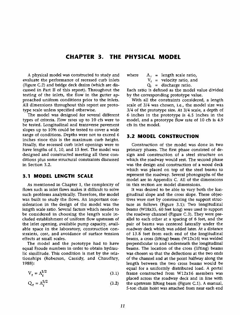
CHAPTER 3. THE PHYSICAL MODEL

A physical model was constructed to study and evaluate the performance of recessed curb inlets (Figure C.2) and bridge deck drains (which are dis­cussed in Part II of this report). Throughout the testing of the inlets, the flow in the gutter ap­proached uniform conditions prior to the inlets. All dimensions throughout this report are proto­type scale unless specified otherwise.

The model was designed for several different types of criteria. Flow rates up to 10 cfs were to be tested. Longitudinal and transverse pavement slopes up to 10% could be tested to cover a wide range of conditions. Depths were not to exceed 6 inches since this is the maximum curb height. Finally, the recessed curb inlet openings were to have lengths of 5, 10, and 15 feet. The model was designed and constructed meeting all these con­ditions plus some structural constraints discussed in Section 3.2.

3.1 MODEL LENGTH SCALE

As mentioned in Chapter 1, the complexity of flows such as inlet flows makes it difficult to solve such problems analytically. Therefore, the model was built to study the flows. An important con­sideration in the design of the model was the length scale ratio. Several factors which needed to be considered in choosing the length scale in­cluded establishment of uniform flow upstream of the inlet opening, available pump capacity, avail­able space in the laboratory, construction con­straints, cost, and avoidance of surface tension effects at small scales.

The model and the prototype had to have equal Froude numbers in order to obtain hydrau­lic similitude. This condition is met by the rela­tionships (Roberson, Cassidy, and Chaudhry, 1988):

V = A112 I I

Q = AS/2 r r

(3.1)

(3.2)

11

where A r = length scale ratio, Vr = velocity ratio, and Q. = discharge ratio.

Each ratio is defined as the model value divided by the corresponding prototype value.

With all the constraints considered, a length scale of 3/4 was chosen, i.e., the model size was 3/4 of the prototype size. At 3/4 scale, a depth of 6 inches in the prototype is 4.5 inches in the model, and a prototype flow rate of 10 cfs is 4.9 cfs in the model.

3.2 MODEL CONSTRUCTION

Construction of the model was done in two primary phases. The first phase consisted of de­sign and construction of a steel structure on which the roadway would rest. The second phase was the design and construction of a wood deck which was placed on top of the steel beams to represent the roadway. Several photographs of the model are in Appendix C. All of the dimensions in this section are model dimensions.

It was desired to be able to vary both the lon­gitudinal slope and the cross slope. These objec­tives were met by constructing the support struc­ture as follows (Figure 3.1): Two longitudinal beams (W18x35, 60 feet long) were used to support the roadway channel (Figure C.3). They were par­allel to each other at a spacing of 6 feet, and the pair of beams was centered laterally under the roadway deck which was added later. At a distance of 13.8 feet from each end of the longitudinal beams, a cross (lifting) beam (W12x16) was welded perpendicular to and underneath the longitudinal beams. The location of the cross (lifting) beams was chosen so that the deflections at the two ends of the channel and at the point halfway along the length between the two cross beams would be equal for a uniformly distributed load. A portal frame constructed from W12x16 members was placed across the roadway deck and in line with the upstream lifting beam (Figure C.1). A manual, 5-ton chain hoist was attached from near each end

Beam

Hoist Hoist

c: E :::l 0 u

Figure 3.1

Curb

Plywood Deck

a) Upstream Portal Frame

Plywood Deck Curb

2x6 joists

longitudinal Beams

lifting Beam

b) Downstream Supports

Schematic diagram of primary struc­tural aspects of roadway model

of the top beam of the portal frame to the top of the upstream lifting beam. On one side of the downstream cross beam, the support was a pivot consisting of a 2-inch ball bearing in seats on top of a short column (Figure C.4). A taller column with a third chain hoist was at the other end of the downstream cross beam (Figure C.1). With the use of the frames, pivot, and manual chain hoists, the longitudinal gutter and transverse pavement slopes could be changed easily.

The structure was designed to allow no more than a 1/8-inch deflection at any location along

12

the roadway for the dead load plus the live load (water plus personnel). This constraint was im­posed to ensure that neither the hydraulics of the flow nor the measurements would be af­fected by deflections or changes in deflections as the amount of water or other loads on the structure changed.

The second phase was a wood deck which was placed on top of the longitudinal steel beams. The wood structure consisted of 2x6 floor joists spaced at longitudinal intervals of 2 feet. A 3/4-inch plywood deck was installed on the joists to be the pavement surface (Figures C.3 and C.4). The deck was subsequently roughened to repre­sent the hydraulic roughness of a pavement (Sec­tion 3.5). The total wood structure was 14 feet wide and 64 feet long. The joists were framed to support a 2-foot overhang at each end of the channel, giving a total length of 64 feet. The curbs were then placed on both sides of the model roadway at a spacing of 10.5 feet, which is the model width of a 14-foot lane. The curbs for the roadway were constructed of painted, wolmanized 2x6's. The roadway deck was wide enough to allow walkways approximately 1.5 feet wide on each side of the roadway. After this con­struction phase was complete, the entire model in contact with water was waterproofed with a liquid sealant (which was also used to attach the roughness elements).

3.3 MODEL LAYOUT

A plan view of the physical model is shown in Figure 3.2. (See also Figure C.Z.) Water was pumped from a half-million-gallon reservoir to the headbox. Immediately downstream of the headbox was a series of baffles to adjust and dampen the flow conditions in the model. The distance from the headbox to the upstream por­tion of the recessed inlet section varied from 26 to 36 feet, depending on the inlet length. For supercritical flow, this distance was long enough to allow the water to reach uniform depth prior to entering the inlet section.

length = 64 ft

~I ~- ;JI 1. length = 26 ft to 36 ft .I )ecesse~ .I (depending on length of inlet section) Inlet Section

Figure 3.2 Plan view of physical model (model dimensions)

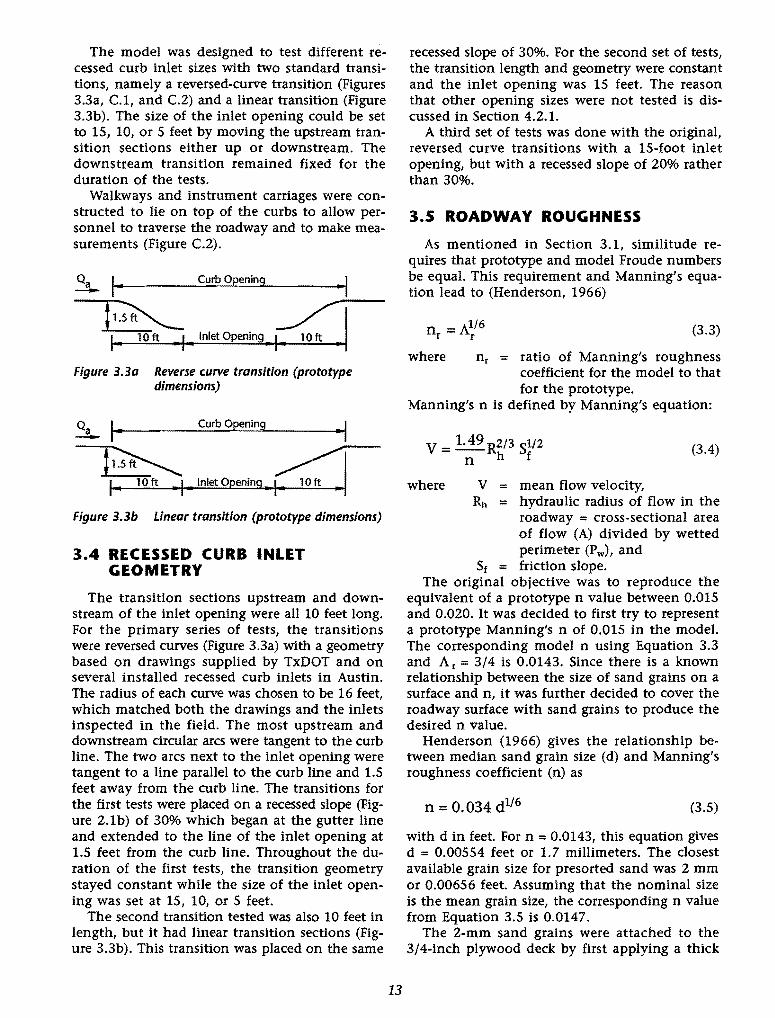
The model was designed to test different re­cessed curb inlet sizes with two standard transi­tions, namely a reversed-curve transition (Figures 3.3a, C.1, and C.2) and a linear transition (Figure 3.3b). The size of the inlet opening could be set to 15, 10, or 5 feet by moving the upstream tran­sition sections either up or downstream. The downstream transition remained fixed for the duration of the tests.

Walkways and instrument carriages were con­structed to lie on top of the curbs to allow per­sonnel to traverse the roadway and to make mea­surements (Figure C.2).

~ I• Curb Opening •I

~ ,lolotOpeolog,~ Figure 3.3a Reverse curve transition (prototype

dimensions)

~ I• Curb Opening •I

~·'""'Op'"l"!!, ~ Figure 3.3b Linear transition (prototype dimensions)

3.4 RECESSED CURB INLET GEOMETRY

The transition sections upstream and down­stream of the inlet opening were all 10 feet long. For the primary series of tests, the transitions were reversed curves (Figure 3.3a) with a geometry based on drawings supplied by TxDOT and on several installed recessed curb inlets in Austin. The radius of each curve was chosen to be 16 feet, which matched both the drawings and the inlets inspected in the field. The most upstream and downstream circular arcs were tangent to the curb line. The two arcs next to the inlet opening were tangent to a line parallel to the curb line and 1.5 feet away from the curb line. The transitions for the first tests were placed on a recessed slope (Fig­ure 2.1b) of 30% which began at the gutter line and extended to the line of the inlet opening at 1.5 feet from the curb line. Throughout the du­ration of the first tests, the transition geometry stayed constant while the size of the inlet open­ing was set at 15, 10, or 5 feet.

The second transition tested was also 10 feet in length, but it had linear transition sections (Fig­ure 3.3b). This transition was placed on the same

13

recessed slope of 30%. For the second set of tests, the transition length and geometry were constant and the inlet opening was 15 feet. The reason that other opening sizes were not tested is dis­cussed in Section 4.2.1.

A third set of tests was done with the original, reversed curve transitions with a 15-foot inlet opening, but with a recessed slope of 20% rather than 30%.

3.5 ROADWAY ROUGHNESS

As mentioned in Section 3.1, similitude re­quires that prototype and model Froude numbers be equaL This requirement and Manning's equa­tion lead to (Henderson, 1966)

n = Al/6 r r (3.3)

where nr = ratio of Manning's roughness coefficient for the model to that for the prototype.

Manning's n is defined by Manning's equation:

(3.4)

where V = mean flow velocity, Rh = hydraulic radius of flow in the

roadway = cross-sectional area of flow (A) divided by wetted perimeter (Pw), and

sf = friction slope. The original objective was to reproduce the

equivalent of a prototype n value between 0.015 and 0.020. It was decided to first try to represent a prototype Manning's n of 0.015 in the modeL The corresponding model n using Equation 3.3 and Ar = 3/4 is 0.0143. Since there is a known relationship between the size of sand grains on a surface and n, it was further decided to cover the roadway surface with sand grains to produce the desired n value.

Henderson (1966) gives the relationship be­tween median sand grain size (d) and Manning's roughness coefficient (n) as

n = 0. 034 d116 (3.5)

with din feet. For n = 0.0143, this equation gives d = 0.00554 feet or 1.7 millimeters. The closest available grain size for presorted sand was 2 mm or 0.00656 feet. Assuming that the nominal size is the mean grain size, the corresponding n value from Equation 3.5 is 0.0147.

The 2-mm sand grains were attached to the 3/4-inch plywood deck by first applying a thick

coat of waterproofing, which also served as an ad­hesive, and then scattering the sand grains uni­formly over the surface. Another coat of water­proofing was applied to secure the sands grains to the surface (Figure C.5).

Experiments were conducted to quantify the re­sulting roughness. First, the recessed inlet section was blocked along the curb line, and then the cross slope was set to zero. The tests were conducted at longitudinal slopes of 0.001, 0.03, and 0.05 with two known discharges for each slope. The water depths were measured at 1/3 points along the length of the roadway. The standard step method (Henderson, 1966) was used to determine n. A spreadsheet was used to generate water surface pro­files for trial values of n. The correct n value was the one which caused the calculated profiles to agree most closely with the measurements. By this procedure Manning's roughness coefficient was de­termined to be 0.019 in the model or 0.020 for the prototype. This n value was confirmed by many measurements made during the tests of inlet capac­ity. It is unknown why the actual Manning's rough­ness was larger than what was calculated from Equa­tion 3.5. Calculations indicated that there is no significant change in n with changing depths for the range of depths in these experiments.

3.6 MEASUREMENTS

During the experimentation, it was necessary to measure the flow rate into the model, the flow rate into the recessed curb inlet, the flow rate passing the inlet section (the carryover), and wa­ter depths on the roadway surface.

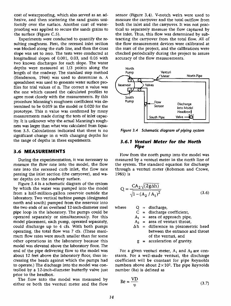
Figure 3.4 is a schematic diagram of the system by which the water was pumped into the model from a half-million-gallon reservoir outside the laboratory. Two vertical turbine pumps (designated north and south) pumped from the reservoir into the two ends of an overhead 12-inch-diameter steel pipe loop in the laboratory. The pumps could be operated separately or simultaneously. For this model placement, each pump, operated separately, could discharge up to 4 cfs. With both pumps operating, the total flow was 7 cfs. (These maxi­mum flow rates were much smaller than for some other operations in the laboratory because this model was elevated above the laboratory floor. The end of the pipe delivering flow to the model was about 12 feet above the laboratory floor, thus in­creasing the heads against which the pumps had to operate.) The discharge into the model was con­trolled by a 12-inch-diameter butterfly valve just prior to the headbox.

The flow into the model was measured by either or both the venturi meter and the flow

14

sensor (Figure 3.4). V-notch weirs were used to measure the carryover and the total outflow from both the inlet and the carryover. It was not prac­tical to separately measure the flow captured by the inlet. Thus, this flow was determined by sub­tracting the carryover from the total flow. All of the flow measurement devices were calibrated at the start of the project, and the calibrations were checked periodically during the project to assure accuracy of the flow measurements.

North Pump

North Pipe

South Pipe

Figure 3.4 Schematic diagram of piping system

3.6. 1 Venturi Meter for the North Pipe

Flow from the north pump into the model was measured by a venturi meter in the north line of the system. The standard equation for discharge through a venturi meter (Roberson and Crowe, 1985) is

Q = CA2 ~(2gMl) ~1-(Az/ Al)2

where Q discharge, C = discharge coefficient,

A1 = area of approach pipe, A2 = area of venturi throat,

(3.6)

ah = difference in piezometric head between the entrance and throat of the venturi, and

g = acceleration of gravity.

For a given venturi meter, A1 and A2 are con­stants. For a well-made venturi, the discharge coefficient will be constant for pipe Reynolds numbers above about 2 x 10s. The pipe Reynolds number (Re) is defined as

Re= VD '\) (3.7)

where V = mean flow velocity, D = diameter, and u = kinematic viscosity.

Since D and u are constant (except for small changes in u due to temperature changes), the dis­charge coefficient should be constant for all veloci­ties greater than a certain value, or, equivalently, for all discharges greater than a certain value.

The venturi in the north pipe has an entrance diameter of 12 inches and a throat diameter of 6 inches. For a venturi meter of this size, the dis­charge coefficient should be constant for throat velocities greater than 2 fps in the 12-inch pipe or for discharges greater than 1.6 cfs. Accordingly, Equation 3.6 can be simplified to

Q =K 8ho.s (3.8)

where K=CA2~2g/[l-(A2 / A1)2].

K should be constant for discharges greater than 1.6 cfs.

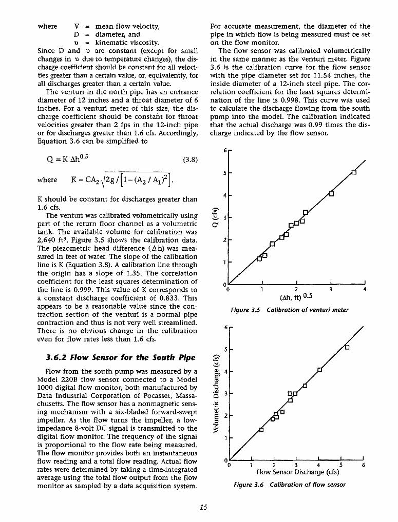
The venturi was calibrated volumetrically using part of the return floor channel as a volumetric tank. The available volume for calibration was 2,640 ft3• Figure 3.5 shows the calibration data. The piezometric head difference (Ah) was mea­sured in feet of water. The slope of the calibration line is K (Equation 3.8). A calibration line through the origin has a slope of 1.35. The correlation coefficient for the least squares determination of the line is 0.999. This value of K corresponds to a constant discharge coefficient of 0.833. This appears to be a reasonable value since the con­traction section of the venturi is a normal pipe contraction and thus is not very well streamlined. There is no obvious change in the calibration even for flow rates less than 1.6 cfs.

3.6.2 Flow Sensor for the South Pipe

Flow from the south pump was measured by a Model 220B flow sensor connected to a Model 1000 digital flow monitor, both manufactured by Data Industrial Corporation of Pocasset, Massa­chusetts. The flow sensor has a nonmagnetic sens­ing mechanism with a six-bladed forward-swept impeller. As the flow turns the impeller, a low­impedance 8-volt DC signal is transmitted to the digital flow monitor. The frequency of the signal is proportional to the flow rate being measured. The flow monitor provides both an instantaneous flow reading and a total flow reading. Actual flow rates were determined by taking a time-integrated average using the total flow output from the flow monitor as sampled by a data acquisition system.

15

For accurate measurement, the diameter of the pipe in which flow is being measured must be set on the flow monitor.

The flow sensor was calibrated volumetrically in the same manner as the venturi meter. Figure 3.6 is the calibration curve for the flow sensor with the pipe diameter set for 11.54 inches, the inside diameter of a 12-inch steel pipe. The cor­relation coefficient for the least squares determi­nation of the line is 0.998. This curve was used to calculate the discharge flowing from the south pump into the model. The calibration indicated that the actual discharge was 0.99 times the dis­charge indicated by the flow sensor.

6

C/

2 3 4

(Llh, ft) 0.5

Figure 3.5 Calibration of venturi meter

6

5

0o 1 2 3 4 5 6 Flow Sensor Discharge (ds)

Figure 3.6 Calibration of flow sensor

3.6.3 V-Notch Weir for the Carryover

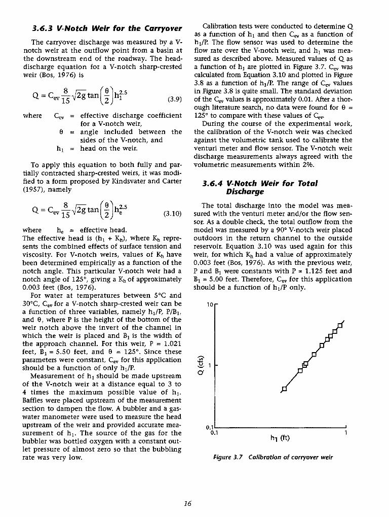
The carryover discharge was measured by a V­notch weir at the outflow point from a basin at the downstream end of the roadway. The head­discharge equation for a V-notch sharp-crested weir (Bos, 1976) is

Q = C ~ rz;:g tan(!)h2·5

ev 15 v"'~ 2 1 (3.9)

where Cev = effective discharge coefficient for a V-notch weir,

e = angle included between the sides of the V-notch, and

hl = head on the weir.

To apply this equation to both fully and par­tially contracted sharp-crested weirs, it was modi­fied to a form proposed by Kindsvater and Carter (1957), namely

Q = cev 185 ~tan(~)h~·5

(3.10)

where he = effective head. The effective head is (h1 + KIJ, where Kh repre­sents the combined effects of surface tension and viscosity. For V-notch weirs, values of Kh have been determined empirically as a function of the notch angle. This particular V-notch weir had a notch angle of 125°, giving a Kh of approximately 0.003 feet (Bos, 1976).

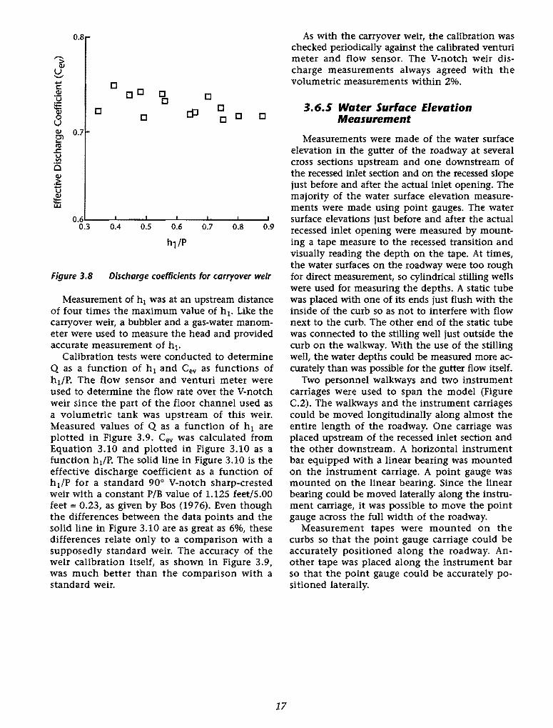
For water at temperatures between soc and 30°C, Cev for a V-notch sharp-crested weir can be a function of three variables, namely h1/P, P/B1,

and e, where P is the height of the bottom of the weir notch above the invert of the channel in which the weir is placed and B1 is the width of the approach channel. For this weir, P = 1.021 feet, B1 = 5.50 feet, and e = 125°. Since these parameters were constant, Cev for this application should be a function of only htfP.

Measurement of h 1 should be made upstream of the V-notch weir at a distance equal to 3 to 4 times the maximum possible value of h 1•

Baffles were placed upstream of the measurement section to dampen the flow. A bubbler and a gas­water manometer were used to measure the head upstream of the weir and provided accurate mea­surement of h 1• The source of the gas for the bubbler was bottled oxygen with a constant out­let pressure of almost zero so that the bubbling rate was very low.

16

Calibration tests were conducted to determine Q as a function of h 1 and then Cev as a function of hifP. The flow sensor was used to determine the flow rate over the V-notch weir, and h1 was mea­sured as described above. Measured values of Q as a function of h 1 are plotted in Figure 3.7. Cev was calculated from Equation 3.10 and plotted in Figure 3.8 as a function of h1/P. The range of Cev values in Figure 3.8 is quite small. The standard deviation of the Cev values is approximately 0.01. After a thor­ough literature search, no data were found for e = 125° to compare with these values of Cev·

During the course of the experimental work, the calibration of the V-notch weir was checked against the volumetric tank used to calibrate the venturi meter and flow sensor. The V-notch weir discharge measurements always agreed with the volumetric measurements within 2%.

3.6.4 V-Notch Weir for Total Discharge

The total discharge into the model was mea­sured with the venturi meter and/or the flow sen­sor. As a double check, the total outflow from the model was measured by a 90° V-notch weir placed outdoors in the return channel to the outside reservoir. Equation 3.10 was used again for this weir, for which Kh had a value of approximately 0.003 feet (Bos, 1976). As with the previous weir, P and B1 were constants with P = 1.125 feet and B1 = 5.00 feet. Therefore, Cev for this application should be a function of h dP only.

Cf

10

~

•

•

• •

• • • •

0.1 ........ ----------------' 0.1

Figure 3.7 Calibration of carryover weir

0.8

'1 u .._, ..... [] s:::: co Q) [] [] ·o [] :£: [] cP

[] Q)

[] [] [] 0 [] u Q) 0.7 El ttl

.£: v ., i5 Q)

:8 Q)

5:i 0.6

0.3 0.4 0.5 0.6 0.7 0.8 0.9

h1/P

Figure 3.8 Discharge coefficients for carryover weir

Measurement of h1 was at an upstream distance of four times the maximum value of h 1• Like the carryover weir, a bubbler and a gas~water manom­eter were used to measure the head and provided accurate measurement of h1•

Calibration tests were conducted to determine Q as a function of h 1 and Cev as functions of hifP. The flow sensor and venturi meter were used to determine the flow rate over the V-notch weir since the part of the floor channel used as a volumetric tank was upstream of this weir. Measured values of Q as a function of h 1 are plotted in Figure 3.9. Cev was calculated from Equation 3.10 and plotted in Figure 3.10 as a function h1/P. The solid line in Figure 3.10 is the effective discharge coefficient as a function of h dP for a standard 90° V~notch sharp-crested weir with a constant P/B value of 1.125 feet/5.00 feet= 0.23, as given by Bos (1976). Even though the differences between the data points and the solid line in Figure 3.10 are as great as 6%, these differences relate only to a comparison with a supposedly standard weir. The accuracy of the weir calibration itself, as shown in Figure 3.9, was much better than the comparison with a standard weir.

17

As with the carryover weir, the calibration was checked periodically against the calibrated venturi meter and flow sensor. The V-notch weir dis­charge measurements always agreed with the volumetric measurements within 2% .

3.6.S Water Surface Elevation Measurement

Measurements were made of the water surface elevation in the gutter of the roadway at several cross sections upstream and one downstream of the recessed inlet section and on the recessed slope just before and after the actual inlet opening. The majority of the water surface elevation measure­ments were made using point gauges. The water surface elevations just before and after the actual recessed inlet opening were measured by mount­ing a tape measure to the recessed transition and visually reading the depth on the tape. At times, the water surfaces on the roadway were too rough for direct measurement, so cylindrical stilling wells were used for measuring the depths. A static tube was placed with one of its ends just flush with the inside of the curb so as not to interfere with flow next to the curb. The other end of the static tube was connected to the stilling well just outside the curb on the walkway. With the use of the stilling well, the water depths could be measured more ac­curately than was possible for the gutter flow itself.

Two personnel walkways and two instrument carriages were used to span the model (Figure C.2). The walkways and the instrument carriages could be moved longitudinally along almost the entire length of the roadway. One carriage was placed upstream of the recessed inlet section and the other downstream. A horizontal instrument bar equipped with a linear bearing was mounted on the instrument carriage. A point gauge was mounted on the linear bearing. Since the linear bearing could be moved laterally along the instru­ment carriage, it was possible to move the point gauge across the full width of the roadway.

Measurement tapes were mounted on the curbs so that the point gauge carriage could be accurately positioned along the roadway. An­other tape was placed along the instrument bar so that the point gauge could be accurately po­sitioned laterally.

> (])

u '-' ..... r:: (]) ·o ~ 0 u (]) O'l ._ <1:5

.J:: u "' i5 (!)

.;:: .......

~ w

10

0.1~------------------------------_.------------------------------~ 0.1

0.65

0.60 tl

tl tl tl

tl

0.55 tl

0.6

10

Figure 3.9 Calibration of 90° total flow weir

tl

tl

CD tl CD tl tl t1 c c c·

0.8 1.0 1.2 1.4 h1/P

3.7 DATA ANALYSIS

A computer spreadsheet was utilized to convert the 3/4-scale model values to prototype values. Input to the spreadsheet included:

1. flow sensor and venturi meter data to calcu­late the flow rate entering the model;

2. carryover V-notch weir and total discharge V­notch weir measurements to calculate the flow of each;

3. water surface elevations to calculate the gut­ter depth for the approach flow;

4. ponded width upstream of the recessed inlet section;

5. depth of flow just before and after the actual inlet opening; and

Figure 3.10 Discharge coefficients for 900 total flow weir

6. gutter depth and ponded width downstream of the recessed inlet section.

18

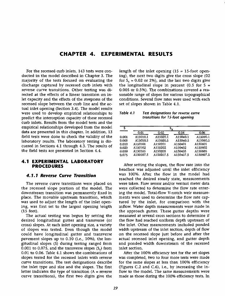
CHAPTER 4. EXPERIMENTAL RESULTS

For the recessed curb inlets, 143 tests were con­ducted in the model described in Chapter 3. The majority of the tests focused on evaluating the discharge captured by recessed curb inlets with reverse curve transitions. Other testing was di­rected at the effects of a linear transition on in­let capacity and the effects of the steepness of the recessed slope between the curb line and the ac­tual inlet opening (Section 3.4). The model results were used to develop empirical relationships to predict the interception capacity of these recessed curb inlets. Results from the model tests and the empirical relationships developed from the model data are presented in this chapter. In addition, 13 field tests were done to check the validity of the laboratory results. The laboratory testing is dis­cussed in Sections 4.1 through 4.3. The results of the field tests are presented in Section 4.4.

4.1 EXPERIMENTAL LABORATORY PROCEDURES

4. 1. 1 Reverse Curve Transition

The reverse curve transitions were placed on the recessed slope portion of the model. The downstream transition was permanently fixed in place. The movable upstream transition, which was used to adjust the length of the inlet open­ing, was first set to the largest opening length (15 feet).

The actual testing was begun by setting the desired longitudinal gutter and transverse (or cross) slopes. At each inlet opening size, a variety of slopes was tested. Even though the model could have longitudinal gutter and transverse pavement slopes up to 0.10 (i.e., 10%), the lon­gitudinal slopes (S) during testing ranged from 0.001 to 0.075, and the transverse slopes (SJ from 0.01 to 0.06. Table 4.1 shows the combinations of slopes tested for the recessed inlets with reverse curve transitions. The test designations describe the inlet type and size and the slopes. The first letter indicates the type of transition (A = reverse curve transitions), the first two digits give the

19

length of the inlet opening (15 = 15-foot open­ing), the next two digits give the cross slope (02 for Sx = 0.02 or 2%), and the last two digits give the longitudinal slope in percent (0.5 for S = 0.005 or 0.5%). The combinations covered a rea­sonable range of slopes for various topographical conditions. Several flow rates were used with each set of slopes shown in Table 4.1.

Table 4.1 Test designations for reverse curve transitions for 1 5-foot opening

s s O.Ql 0.02 0.04 0.06

0.001 A15010.1 A15020.1 A15040.1 A15060.1 0.005 A15010.5 A15020.5 A15040.5 A15060.5 0.010 A150101 A150201 A150401 A150601 0.020 A150102 A150202 A150402 A150602 0.050 A150105 A150205 A150405 A150605 0.075 A150107.5 A150207.5 A150407.5 A150607.5

After setting the slopes, the flow rate into the headbox was adjusted until the inlet efficiency was 100%. After the flow in the model had reached the desired steady state, measurements were taken. Flow sensor and/or venturi meter data were collected to determine the flow rate enter­ing the model. Total-flow V-notch weir measure­ments were used to determine the flow rate cap­tured by the inlet, for comparison with the inflow. Water depth measurements were made in the approach gutter. These gutter depths were measured at several cross sections to determine if the flow had reached uniform depth upstream of the inlet. Other measurements included ponded width upstream of the inlet section, depth of flow on the recessed slope just before and after the actual recessed inlet opening, and gutter depth and ponded width downstream of the recessed inlet section.

After the 100% efficiency test for the set slopes was completed, two to four more tests were made for the same slopes at less than 100% efficiency (Figures C.2 and C.6), i.e., by increasing the in­flow to the model. The same measurements were made as those during the 100% efficiency tests. In

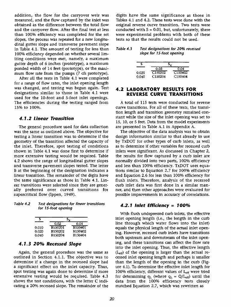
addition, the flow for the carryover weir was measured, and the flow captured by the inlet was obtained as the difference between the total flow and the carryover flow. After the final test at less than 100% efficiency was completed for the set slopes, the process was repeated for a new longitu­dinal gutter slope and transverse pavement slope in Table 4.1. The amount of testing for less than 100% efficiency depended on whether several lim­iting conditions were met, namely, a maximum gutter depth of 6 inches (prototype), a maximum ponded width of 14 feet (prototype), or the maxi­mum flow rate from the pumps (7 cfs prototype).

After all the tests in Table 4.1 were completed for a range of flow rates, the inlet opening length was changed, and testing was begun again. Test designations similar to those in Table 4.1 were used for the 10-foot and 5-foot inlet openings. The efficiencies during the testing ranged from 15% to 100%.

4. 1.2 Linear Transition

The general procedure used for data collection was the same as outlined above. The objective for testing a linear transition was to determine if the geometry of the transition affected the capacity of the inlet. Therefore, spot testing of conditions shown in Table 4.1 was done first to determine if more extensive testing would be required. Table 4.2 shows the range of longitudinal gutter slopes and transverse pavement slopes tested. The letter B at the beginning of the designation indicates a linear transition. The remainder of the digits have the same significance as those in Table 4.1. Lin­ear transitions were selected since they are gener­ally preferred over curved transitions for supercritical flow (Ippen, 1949).

Table 4.2 Test designations for linear transitions for 15-foot opening

s

0.010 0.020 0.040

0.02 Bl50201 B150202 Bl50204

0.04 Bl50401 Bl50402 Bl50404

4. 1. 3 20% Recessed Slope

Again, the general procedure was the same as outlined in Section 4.1.1. The objective was to determine if a change in the recessed slope had a significant effect on the inlet capacity. Thus, spot testing was again done to determine if more extensive testing would be required. Table 4.3 shows the test conditions, with the letter C indi­cating a 20% recessed slope. The remainder of the

20

digits have the same significance as those in Tables 4.1 and 4.2. These tests were done with the original reverse curve transition. Two tests were conducted with S = 0.01, but, unfortunately, there were experimental problems with both of these tests so that the results could not be used.

Table 4.3 Test designations for 20% recessed slope for 15-foot opening

s

0.020 0.040

0.02 Cl50202 Cl50204

0.04 C150402 C150404

4.2 LABORATORY RESULTS FOR REVERSE CURVE TRANSITIONS

A total of 115 tests were conducted for reverse curve transitions. For all of these tests, the transi­tion length and transition geometry remained con­stant while the size of the inlet opening was set to 15, 10, or 5 feet. Data from the model experiments are presented in Table A.1 in Appendix A.

The objective of the data analysis was to obtain design information similar to that already in use by TxDOT for other types of curb inlets, as well as to determine if other variables for recessed curb inlets were significant. As discussed in Chapter 2, the results for flow captured by a curb inlet are normally divided into two parts, 100% efficiency and less than 100% efficiency. TxDOT uses equa­tions similar to Equation 2.7 for 100% efficiency and Equation 2.6 for less than 100% efficiency for flush inlets. Therefore, analysis of the recessed curb inlet data was first done in a similar man­ner, and then other approaches were evaluated for possible improvements in accuracy of correlations.

4.2.1 Inlet Efficiency = 100%

With flush undepressed curb inlets, the effective inlet opening length (i.e., the length in the curb line through which water flows into the inlet) equals the physical length of the actual inlet open­ing. However, recessed curb inlets have transitions both upstream and downstream of the inlet open­ing, and these transitions can affect the flow rate into the inlet opening. Thus, the effective length (Leff) of the opening is larger than the actual re­cessed inlet opening length and perhaps is smaller than the length of the opening in the curb (Fig­ure 4.1). To determine the effective inlet length for 100% efficiency, different values of Leff were tried for determining qL (where qL = Q/Leff) until the data from the 100% efficiency tests closely matched Equation 2. 7, which was rewritten as

where

(4.1)

qL = flow per ft of inlet (cfs/ft) at 100% efficiency = Q/Leff,

y = flow depth in approach gutter (ft), and

Q = Oa (i.e., inlet flow = approach flow for 100% efficiency).

Figure 4.1 Plan view of inlet section

For all three inlet opening lengths (5, 10, and 15 feet), the optimum length of the effective in­let opening to match Equation 4.1 was the full upstream transition (10 feet) plus the full inlet opening plus 8 feet of the downstream transition. That is, the 5-, 10-, and 15-foot inlets were effec­tively 23, 28, and 33 feet long at 100% efficiency. Thus, any flow that entered the last 2 feet of the transition ultimately flowed downstream as carryover rather than back into the inlet. On the other hand, flow that entered the first 8 feet of the downstream transition actually turned around and flowed back upstream into the inlet opening. These conclusions are consistent with visual ob­servations during the tests for 100% efficiency.

When qL was first plotted against the measured depth (y) of flow in the gutter, there was a large amount of scatter because of normal random er­rors in the measured y values due to surface waves affecting the point gauge readings. The scatter was reduced significantly if the gutter depths were determined from Manning's equation (Equation 2.22) using the measured values of Oa, n, S and Sx. TxDOT uses this equation to calculate depths in the approach gutter. To be consistent with the present TxDOT methods and to reduce the scat­ter in the data, the analysis of the recessed curb inlets was based on calculated depths.

Figure 4.2 shows Equation 4.1 and the data collected for the reverse curve transition using calculated y values. The standard error of the data relative to Equation 4.1 is 0.026 cfs/ft.

Dividing both sides of Equation 4.1 by .[g to make it dimensionally correct and using the defi­nition of qL allows Equation 4.1 to be rewritten in the same form as Equation 2.15, namely

~=0.124 YLeff gy (4.2)

21

0.30

:E' :]! 0.10 ~

in ::::::: 0.05 CJ II ...J 0"

Lett (ft) a 33 028 •23

0

0.01 ...._ _ _,_ ____ ...._ ___ __,_ ___ _,

0.07 0.10 0.20 0.40 0.70 y (calculated) (ft)

Figure 4.2 Capacity of recessed inlets with reverse curve transitions for efficiency = 100%

The left-hand side of Equation 4.2 is the dimen­sionless flow rate (Q') into the inlet. Thus, the data indicate that this Q' is constant for the 100% capacity tests for the recessed curb inlets. The same is true for flush curb inlets since Equation 4.1 is applicable for flush inlets when qL is de­fined based on the actual inlet length. (Compare Table 2.1.) Even though Q' can also be interpreted as a type of Froude number, it is not the tradi­tional open channel Froude number because of Lett in the denominator. However, Equation 4.2 can be rearranged to give

L Fr =0.351T (4.3)

where T = ponded width = y!Sx. Fr is the traditional open channel Froude number defined as

(4.4)

This definition is based on having the length scale equal to the hydraulic mean depth, which is y/2 for flow in a triangular cross section; the flow area is yT/2 in Equation 4.4.

Equation 4.3 is valid only for 100% efficiency. This equation says that the Froude number for the approach flow for the. condition of 100% effi­ciency increases as LetdT increases, or that increas­ing Leff/T allows the inlet to capture all of the flow for larger and larger Froude numbers. This kind of relationship might be expected since the Froude number can be interpreted as the ratio of the inertial force, which is trying to carry the flow

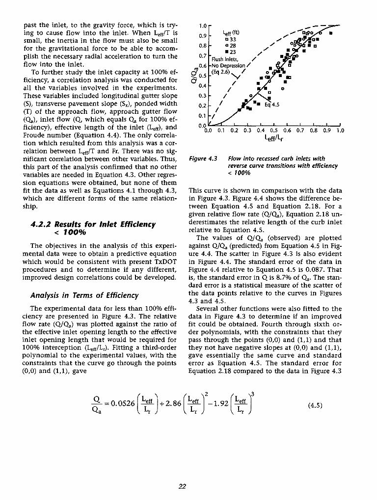
past the inlet, to the gravity force, which is try­ing to cause flow into the inlet. When LetdT is small, the inertia in the flow must also be small for the gravitational force to be able to accom­plish the necessary radial acceleration to turn the flow into the inlet.

To further study the inlet capacity at 100% ef­ficiency, a correlation analysis was conducted for all the variables involved in the experiments. These variables included longitudinal gutter slope (S), transverse pavement slope (SJ, ponded width (T) of the approach flow, approach gutter flow (<l.a), inlet flow (Q, which equals <l.a for 100% ef­ficiency), effective length of the inlet (Letf), and Froude number (Equation 4.4). The only correla­tion which resulted from this analysis was a cor­relation between Leff/T and Fr. There was no sig­nificant correlation between other variables. Thus, this part of the analysis confirmed that no other variables are needed in Equation 4.3. Other regres­sion equations were obtained, but none of them fit the data as well as Equations 4.1 through 4.3, which are different forms of the same relation­ship.

4.2.2 Results for Inlet Efficiency < JOO%

The objectives in the analysis of this experi­mental data were to obtain a predictive equation which would be consistent with present TxDOT procedures and to determine if any different, improved design correlations could be developed.

Analysis in Terms of Efficiency

The experimental data for less than 100% effi­ciency are presented in Figure 4.3. The relative flow rate (QJ<l.a) was plotted against the ratio of the effective inlet opening length to the effective inlet opening length that would be required for 100% interception (LetdLr)· Fitting a third-order polynomial to the experimental values, with the constraints that the curve go through the points (0,0) and (1,1), gave

22

1.0

0.9 leff (ft) ..... /

1:133 / 0.8 028 /

•23 / 0.7 /

Flush Inlets, / ~0.6 No Depression /

f!o.s (Eq2.6)v/

CJ / 0.4 I 0

0.3 I 0.2 I

I 0.1 I 0.0 "-::::;.&..-....L....---1-_.__....___.__....~----l"---'----'

0.0 0.1 0.2 0.3 0.4 0.5 0.6 0.7 0.8 0.9 1.0

Lett!Lr

Figure 4.3 Flow into recessed curb inlets with reverse curve transitions with efficiency < 100%

This curve is shown in comparison with the data in Figure 4.3. Figure 4.4 shows the difference be­tween Equation 4.5 and Equation 2.18. For a given relative flow rate (QJ<l.a), Equation 2.18 un­derestimates the relative length of the curb inlet relative to Equation 4.5.

The values of QJ<l.a (observed) are plotted against QJ<l.a (predicted) from Equation 4.5 in Fig­ure 4.4. The scatter in Figure 4.3 is also evident in Figure 4.4. The standard error of the data in Figure 4.4 relative to Equation 4.5 is 0.087. That is, the standard error in Q is 8.7% of <l.a. The stan­dard error is a statistical measure of the scatter of the data points relative to the curves in Figures 4.3 and 4.5.

Several other functions were also fitted to the data in Figure 4.3 to determine if an improved fit could be obtained. Fourth through sixth or­der polynomials, with the constraints that they pass through the points (0,0) and (1,1) and that they not have negative slopes at (0,0) and (1,1), gave essentially the same curve and standard error as Equation 4.5. The standard error for Equation 2.18 compared to the data in Figure 4.3

(4.5)

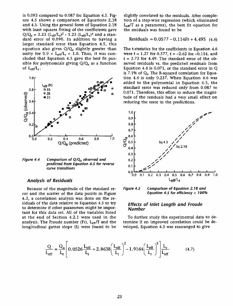
is 0.093 compared to 0.087 for Equation 4.5. Fig­ure 4.5 shows a comparison of Equations 2.18 and 4.5. Using the general form of Equation 2.18 with least squares fitting of the coefficients gave Q/O,a_ = 2.23 (Leff/Lr)2 - 1.23 (Leff1Lr)4 and a stan­dard error of 0.090. In addition to having a larger standard error than Equation 4.5, this equation also gives Q/o.a slightly greater than unity for 0.9 < Leff/Lr < 1.0. Thus, it was con­cluded that Equation 4.5 gave the best fit pos­sible for polynomials giving Q/O,a_ as a function of Leff/Lr.

1.0

0.8 -'"0

~ Q) 0.6 ~ s c!J 0.4 -0

0.2 D

leff (ft) D 33 028 •23

0

0

D

0.2 0.4 0.6 0.8 1 .0 Q/Oa (predicted)

Figure 4.4 Comparison of Q!Qa observed and predicted from Equation 4.5 for reverse curve transitions

Analysis of Residuals

Because of the magnitude of the standard er­ror and the scatter of the data points in Figure 4.3, a correlation analysis was done on the re­siduals of the data relative to Equation 4.5 to try to determine if other parameters might be impor­tant for this data set. All of the variables listed at the end of Section 4.2.1 were used in the analysis. The Froude number (Fr), 4ff/T and the longitudinal gutter slope (S) were found to be

23

slightly correlated to the residuals. After comple­tion of a step-wise regression (which eliminated LettiT as a parameter), the best fit equation for the residuals was found to be

Residuals = 0.0577- 0.114Fr + 4.49S (4.6)

The t-statistics for the coefficients in Equation 4.6 were t = 1.27 for 0.577, t = -2.62 for -0.114, and t = 3.72 for 4.49. The standard error of the ob­served residuals vs. the predicted residuals from Equation 4.6 is 0.071, or the standard error in Q is 7.1% of o.a_. The R-squared correlation for Equa­tion 4.6 is only 0.237. When Equation 4.6 was added to the polynomial in Equation 4.5, the standard error was reduced only from 0.087 to 0.071. Therefore, this effort to reduce the magni­tude of the residuals had a very small effect on reducing the error in the predictions.

1.0

n:s 0.6 CJ .._ 0.5 CJ

0.4

0.3

0.2

0.1

0.0 r..&.::J....-....L.----1-....L..-.&..---L.-..L.----1 ...... -L.---s 0.0 0.1 0.2 0.3 0.4 0.5 0.6 0.7 0.8 0.9 1.0

Lettllr

Figure 4.5 Comparison of Equation 2.18 and Equation 4.5 for efficiency < 1 00%

Effects of Inlet Length and Froude Number

To further study the experimental data to de­termine if an improved correlation could be de­veloped, Equation 4.5 was rearranged to give

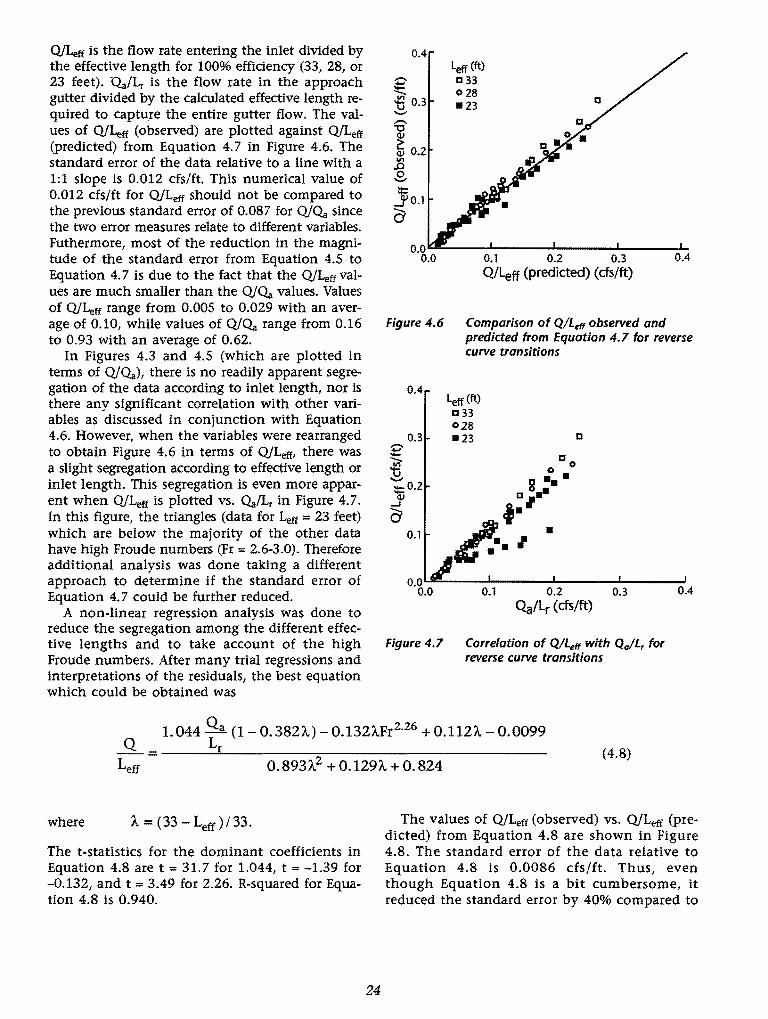
Q/Lett is the flow rate entering the inlet divided by the effective length for 100% efficiency (33, 28, or 23 feet). Oa/Lr is the flow rate in the approach gutter divided by the calculated effective length re­quired to capture the entire gutter flow. The val­ues of Q/Leff (observed) are plotted against Q/Leff (predicted) from Equation 4.7 in Figure 4.6. The standard error of the data relative to a line with a 1:1 slope is 0.012 cfs/ft. This numerical value of 0.012 cfs/ft for Q/Leff should not be compared to the previous standard error of 0.087 for Q/0.0. since the two error measures relate to different variables. Futhermore, most of the reduction in the magni­tude of the standard error from Equation 4.5 to Equation 4. 7 is due to the fact that the Q/Letf val­ues are much smaller than the Q/0.0. values. Values of Q/Leff range from 0.005 to 0.029 with an aver­age of 0.10, while values of Q/0.0. range from 0.16 to 0.93 with an average of 0.62.

In Figures 4.3 and 4.5 (which are plotted in terms of Q/0.0.), there is no readily apparent segre­gation of the data according to inlet length, nor is there any significant correlation with other vari­ables as discussed in conjunction with Equation 4.6. However, when the variables were rearranged to obtain Figure 4.6 in terms of Q/Leff, there was a slight segregation according to effective length or inlet length. This segregation is even more appar­ent when Q/Leff is plotted vs. Oa/Lr in Figure 4.7. In this figure, the triangles (data for Lett = 23 feet) which are below the majority of the other data have high Froude numbers (Fr = 2.6-3.0). Therefore additional analysis was done taking a different approach to determine if the standard error of Equation 4. 7 could be further reduced.

A non-linear regression analysis was done to reduce the segregation among the different effec­tive lengths and to take account of the high Froude numbers. After many trial regressions and interpretations of the residuals, the best equation which could be obtained was

0.4

-E -tl 0.3 -:.0 ~ Q,) 0.2 ~ .£, :;:

_jl0.1

?J

Figure 4.6

0.4

0.3 E'

~ :;: 0.2 Q,)

....J

?J 0.1

lett (ft) c 33 028 •23

0.1 0.2 0.3 0.4 Q/Leff (predicted) (ds/ft)

Comparison of Q/Leff observed and predicted from Equation 4.7 for reverse curve transitions

Leff (ft) c 33 028 •23 c

O.OL.'Iil::'-----'-----'----...r....--~ 0.0 0.1 0.2 0.3 0.4

Figure 4.7

Qa/Lr ( ds/ft)

Correlation of Q/Leff with Qo/L, for reverse curve transitions

1.044 Qa (1-0.382A.)-0.132A.Fr2·26 +0.112A.-0.0099 Q Lr --=---""""-------=--------------

0. 893A.2 + 0.129A. + 0. 824 (4.8)

where A.= (33- Leff) I 33.

The t-statistics for the dominant coefficients in Equation 4.8 are t = 31.7 for 1.044, t = -1.39 for -0.132, and t = 3.49 for 2.26. R-squared for Equa­tion 4.8 is 0.940.

24

The values of Q/Lett (observed) vs. Q/Leff (pre­dicted) from Equation 4.8 are shown in Figure 4.8. The standard error of the data relative to Equation 4.8 is 0.0086 cfs/ft. Thus, even though Equation 4.8 is a bit cumbersome, it reduced the standard error by 40% compared to

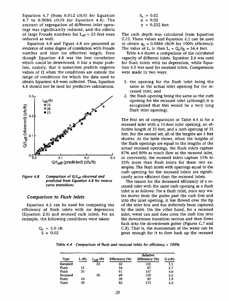
Equation 4. 7 (from 0.012 cfs/ft for Equation 4. 7 to 0.0086 cfs/ft for Equation 4.8). The amount of segregation of different inlet open­ings was significantly reduced, and the effects of large Froude numbers for Lett = 23 feet were reduced as well.

Equation 4.8 and Figure 4.8 are presented as evidence of some degree of correlation with Froude number and inlet (or effective) length. Even though Equation 4.8 was the best correlation which could be determined, it has a major prob­lem, namely, that it sometimes predicts negative values of Q when the conditions are outside the range of conditions for which the data used to obtain Equation 4.8 were collected. Thus, Equation 4.8 should not be used for predictive calculations.

0.3 lett (ft) 1:133 028 •23

0.1 0.2 0.3

Q/leff (predicted) (ds/ft)

Figure 4.8 Comparison of Q/Leff observed and predicted from Equation 4.8 for reverse curve transitions

Comparison to Flush Inlets

Equation 4.5 can be used for comparing the efficiency of flush inlets with no depression (Equation 2.6) and recessed curb inlets. For an example, the following conditions were taken:

<la = 5.0 cfs s = 0.02

Sx = 0.02 n = 0.02 y = 0.252 feet

The curb depth was calculated from Equation 2.22. These values and Equation 4.1 can be used to obtain qL = 0.0886 cfs/ft for 100% efficiency. The value of Lr is then Lr = <la/qL = 56.4 feet.

Table 4.4 shows a comparison of the calculated capacity of different inlets. Equation 2.6 was used for flush inlets with no depression, while Equa­tion 4.5 was used for recessed inlets. Comparisons were made in two ways:

1. the opening for the flush inlet being the same as the actual inlet opening for the re­cessed inlet, and

2. the flush opening being the same as the curb opening for the recessed inlet (although it is recognized that this would be a very long flush inlet opening).

The first set of comparisons in Table 4.4 is for a recessed inlet with a 15-foot inlet opening, an ef­fective length of 33 feet, and a curb opening of 35 feet. For the second set, all of the lengths are 5 feet shorter. As the table shows, when the lengths of the flush openings are equal to the lengths of the actual recessed openings, the flush inlets capture 87% and 80% as much flow as the recessed inlet, or conversely, the recessed inlets capture 15% to 25% more than flush inlets for these two ex­amples. The flush inlets with openings equal to the curb opening for the recessed inlets are signifi­cantly more efficient than the recessed inlets.

The reason for the decreased efficiency of a re­cessed inlet with the same curb opening as a flush inlet is as follows: For a flush inlet, once any wa­ter moves from the gutter past the curb line and into the inlet opening, it has flowed over the lip of the inlet box and has definitely been captured by the inlet. On the other hand, for a recessed inlet, water can and does cross the curb line into the downstream transition section and then flows back into the downstream gutter (Figures C.7 and C.8). That is, the momentum of the water can be great enough for it to flow back up the recessed

Table 4.4 Comparison of flush and recessed inlets for efficiency < 100%

Relative Type L (ft) Leff (ft) Efficiency(%) Efficiency(%) Q (cfs)

Recessed 33 62 100 3.1 Flush 15 54 87 2.7 Flush 35 91 147 4.6 Recessed 28 49 100 2.5 Flush 10 39 80 1.9 Flush 30 85 173 4.3

25

slope in the downstream transition section and back into the gutter, rather than turning in the downstream transition section and basically flow­ing back upstream to get into the inlet opening as happens for IOO% efficiency. This type of sweep-out exists for all flow conditions but should be expected to be greater as the Froude number of the gutter flow increases.

Another way of viewing the situation is that the effective lengths of the recessed inlets de­crease as the Froude number for the approach flow increases. In a sense, this is the effect that causes the data in Figure 4.3 to be significantly below the curve for flush inlets. Thus, another possible approach for analyzing the data for less than IOO% efficiency might be to use Equation 2.6 rather than Equation 4.5 and then to calcu­late a value of Letf for each flow condition with an efficiency of less than IOO%. For predictive purposes, these values of Leff would then need to be correlated with gutter flow conditions (as rep­resented by Fr and possibly also S, Sx, etc.). In a sense, this alternative approach might be more representative of the hydraulic conditions since reductions in Leff would correspond to flow sweeping out of the downstream part of the re­cessed section. Nevertheless, this alternate ap­proach was not investigated both because it would be more cumbersome than just using Equa­tion 4.5 and because using Equation 4.S is more consistent with the present TxDOT approach of using Equation 2.6 for flush inlets.

4.3 LABORATORY RESULTS FOR LINEAR TRANSI"riONS

Fifteen tests were conducted to investigate the effects of a linear transition on curb inlet capac­ity as compared to the reverse curve transition. For all of these tests, the length of each transition section was 10 feet, and the inlet opening was 15 feet long. The objective of these tests was to de­termine if linear transitions cause a significant change in the hydraulic behavior of recessed in­lets compared to reverse curve transitions. The data (Table A.2, Appendix A) were evaluated pri­marily by comparison to the relationships devel­oped for the recessed inlets with reverse curve transition sections.

4.3.1 Inlet Efficiency = JOO%

In the analysis of the data for 100% efficiency, different effective lengths (Leff) were tried until the data closely matched Equation 4.1. This is

26

the same approach that was used with the data for reverse curve transitions. Using calculated depths as before, the effective length of the IS-foot inlet opening was the full upstream tran­sition plus the inlet opening plus the full down­stream transition. Therefore, with a linear tran­sition, a IS-foot inlet opening was effectively a 3S-foot inlet at IOO% efficiency. Thus, the linear transition is slightly more effective at turning the water which enters the most downstream part of the transition and causing this water to flow back upstream and into the inlet opening at IOO% efficiency. The experimental data for 100% efficiency are presented in Figure 4.9. The stan­dard error of Equation 4.I compared to the lin­ear transition data is O.OOS cfs/ft.

0.30

2 ~ 0.10 -~ ~ 0.05 0' II ...J C"'

0.20 0.40 0.70 y (calculated) (ft)

Figure 4.9 Capacity of recessed inlets with linear transitions for efficiency = 100%

4.3.2 Inlet Efficiency < JOO%

The data for the linear transition with less than IOO% efficiency were analyzed in the same man­ner as the data for the reverse curve transition. The relative flow rate was compared to Leff/Lv i.e., the effective inlet length divided by the effective inlet length required for IOO% interception. The experimental data agree with Equation 4.S rather well using Leff = 35 feet (Figure 4.IO). The stan­dard error of the Q/0... data for the linear transi­tion compared to Equation 4.5 is 0.054. Because of this small standard error, it was concluded that more extensive testing with linear transitions was not justified and that Equations 4.I and 4.5 can be used for linear transitions if the effective lengths of the openings include the full IO feet of the downstream transition, rather than only 8 feet as for reverse curve transitions.

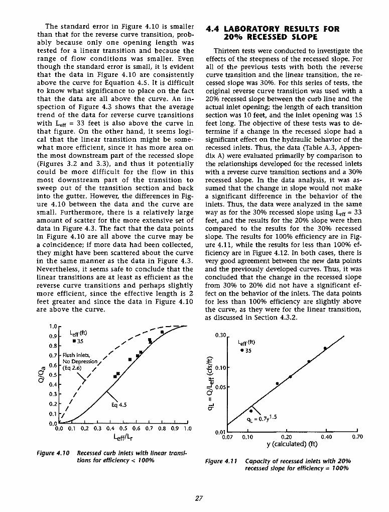
The standard error in Figure 4.10 is smaller than that for the reverse curve transition, prob­ably because only one opening length was tested for a linear transition and because the range of flow conditions was smaller. Even though the standard error is small, it is evident that the data in Figure 4.10 are consistently above the curve for Equation 4.5. It is difficult to know what significance to place on the fact that the data are all above the curve. An in­spection of Figure 4.3 shows that the average trend of the data for reverse curve transitions with Leff = 33 feet is also above the curve in that figure. On the other hand, it seems logi­cal that the linear transition might be some­what more efficient, since it has more area on the most downstream part of the recessed slope (Figures 3.2 and 3.3), and thus it potentially could be more difficult for the flow in this most downstream part of the transition to sweep out of the transition section and back into the gutter. However, the differences in Fig­ure 4.10 between the data and the curve are small. Furthermore, there is a relatively large amount of scatter for the more extensive set of data in Figure 4.3. The fact that the data points in Figure 4.10 are all above the curve may be a coincidence; if more data had been collected, they might have been scattered about the curve in the same manner as the data in Figure 4.3. Nevertheless, it seems safe to conclude that the linear transitions are at least as efficient as the reverse curve transitions and perhaps slightly more efficient, since the effective length is 2 feet greater and since the data in Figure 4.10 are above the curve.

1.0 Left (ft) .,....

0.9 .,.... •35 /

/ 0.8 / / 0.7 Flush Inlets, /

«< 0.6 No Depression/ (Eq 2.6) /

Q 0.5 )/ Cf 0.4

I 0.3 I 0.2

I I

0.1 I 0.0 "-:::::1...-1...-_.L..---L..-._.L..---JL..-.....I----JI..-.....I--....I

0.0 0.1 0.2 0.3 0.4 0.5 0.6 0.7 0.8 0.9 1 .0

'-eff/Lr

Figure 4.10 Recessed curb inlets with linear transi­tions for efficiency < 1 00%

27

4.4 LABORATORY RESULTS FOR 200/o RECESSED SLOPE

Thirteen tests were conducted to investigate the effects of the steepness of the recessed slope. For all of the previous tests with both the reverse curve transition and the linear transition, the re­cessed slope was 30%. For this series of tests, the original reverse curve transition was used with a 20% recessed slope between the curb line and the actual inlet opening; the length of each transition section was 10 feet, and the inlet opening was 15 feet long. The objective of these tests was to de­termine if a change in the recessed slope had a significant effect on the hydraulic behavior of the recessed inlets. Thus, the data (Table A.3, Appen­dix A) were evaluated primarily by comparison to the relationships developed for the recessed inlets with a reverse curve transition sections and a 30% recessed slope. In the data analysis, it was as­sumed that the change in slope would not make a significant difference in the behavior of the inlets. Thus, the data were analyzed in the same way as for the 30% recessed slope using Leff = 33 feet, and the results for the 20% slope were then compared to the results for the 30% recessed slope. The results for 100% efficiency are in Fig­ure 4.11, while the results for less than 100% ef­ficiency are in Figure 4.12. In both cases, there is very good agreement between the new data points and the previously developed curves. Thus, it was concluded that the change in the recessed slope from 30% to 20% did not have a significant ef­fect on the behavior of the inlets. The data points for less than 100% efficiency are slightly above the curve, as they were for the linear transition, as discussed in Section 4.3.2.

0.30 Lett<ft) • 35

g J::! 0.10 ~

J -0.05 Cf II ....I 0"'

0.01.___ ........ ____ _,_ ____ _,_ __ __,

O.Q7 0.10 0.20 0.40 0.70 y (calculated) (ft)

Figure 4.11 Capacity of recessed inlets with 20% recessed slope for efficiency = 1 00%

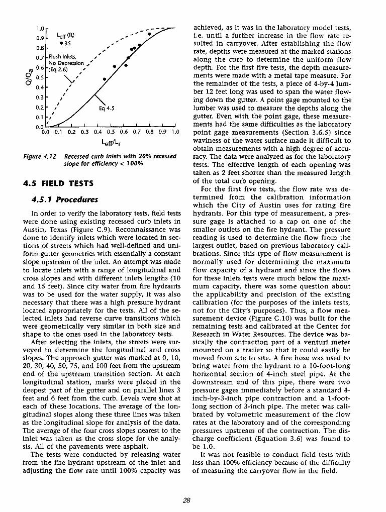
0.7 Flush Inlets, ,. "'

nz 0.6

Q 0.5 C/

0.4

0.3

0.2

No Depression ,. ' (Eq 2.6) , ,

I I

'v' I

I I

, ,

0.1 I I

; ;

.. , ,

0.0 J....o:::L-..L.-.....L--'--.......1--'-----''----'--'-----'

0.0 0.1 0.2 0.3 0.4 0.5 0.6 0.7 0.8 0.9 1.0

Leffllr

Figure 4. 12 Recessed curb inlets with 20% recessed slope for efficiency < 1 00%

4.5 Fl ELD TESTS

4.5. 1 Procedures

In order to verify the laboratory tests, field tests were done using existing recessed curb inlets in Austin, Texas (Figure C.9). Reconnaissance was done to identify inlets which were located in sec­tions of streets which had well-defined and uni­form gutter geometries with essentially a constant slope upstream of the inlet. An attempt was made to locate inlets with a range of longitudinal and cross slopes and with different inlets lengths (10 and 15 feet). Since city water from fire hydrants was to be used for the water supply, it was also necessary that there was a high pressure hydrant located appropriately for the tests. All of the se­lected inlets had reverse curve transitions which were geometrically very similar in both size and shape to the ones used in the laboratory tests.

After selecting the inlets, the streets were sur­veyed to determine the longitudinal and cross slopes. The approach gutter was marked at 0, 10, 20, 30, 40, 50, 75, and 100 feet from the upstream end of the upstream transition section. At each longitudinal station, marks were placed in the deepest part of the gutter and on parallel lines 3 feet and 6 feet from the curb. Levels were shot at each of these locations. The average of the lon­gitudinal slopes along these three lines was taken as the longitudinal slope for analysis of the data. The average of the four cross slopes nearest to the inlet was taken as the cross slope for the analy­sis. All of the pavements were asphalt.

The tests were conducted by releasing water from the fire hydrant upstream of the inlet and adjusting the flow rate until 100% capacity was

28

achieved, as it was in the laboratory model tests, i.e. until a further increase in the flow rate re­sulted in carryover. After establishing the flow rate, depths were measured at the marked stations along the curb to determine the uniform flow depth. For the first five tests, the depth measure­ments were made with a metal tape measure. For the remainder of the tests, a piece of 4-by-4 lum­ber 12 feet long was used to span the water flow­ing down the gutter. A point gage mounted to the lumber was used to measure the depths along the gutter. Even with the point gage, these measure­ments had the same difficulties as the laboratory point gage measurements (Section 3.6.5) since waviness of the water surface made it difficult to obtain measurements with a high degree of accu­racy. The data were analyzed as for the laboratory tests. The effective length of each opening was taken as 2 feet shorter than the measured length of the total curb opening.

For the first five tests, the flow rate was de­termined from the calibration information which the City of Austin uses for rating fire hydrants. For this type of measurement, a pres­sure gage is attached to a cap on one of the smaller outlets on the fire hydrant. The pressure reading is used to determine the flow from the largest outlet, based on previous laboratory cali­brations. Since this type of flow measurement is normally used for determining the maximum flow capacity of a hydrant and since the flows for these inlets tests were much below the maxi­mum capacity, there was some question about the applicability and precision of the existing calibration (for the purposes of the inlets tests, not for the City's purposes). Thus, a flow mea­surement device {Figure C.lO) was built for the remaining tests and calibrated at the Center for Research in Water Resources. The device was ba­sically the contraction part of a venturi meter mounted on a trailer so that it could easily be moved from site to site. A fire hose was used to bring water from the hydrant to a 10-foot-long horizontal section of 4-inch steel pipe. At the downstream end of this pipe, there were two pressure gages immediately before a standard 4-inch-by-3-inch pipe contraction and a !-foot­long section of 3-inch pipe. The meter was cali­brated by volumetric measurement of the flow rates at the laboratory and of the corresponding pressures upstream of the contraction. The dis­charge coefficient (Equation 3.6) was found to be 1.0.

It was not feasible to conduct field tests with less than 100% efficiency because of the difficulty of measuring the carryover flow in the field.

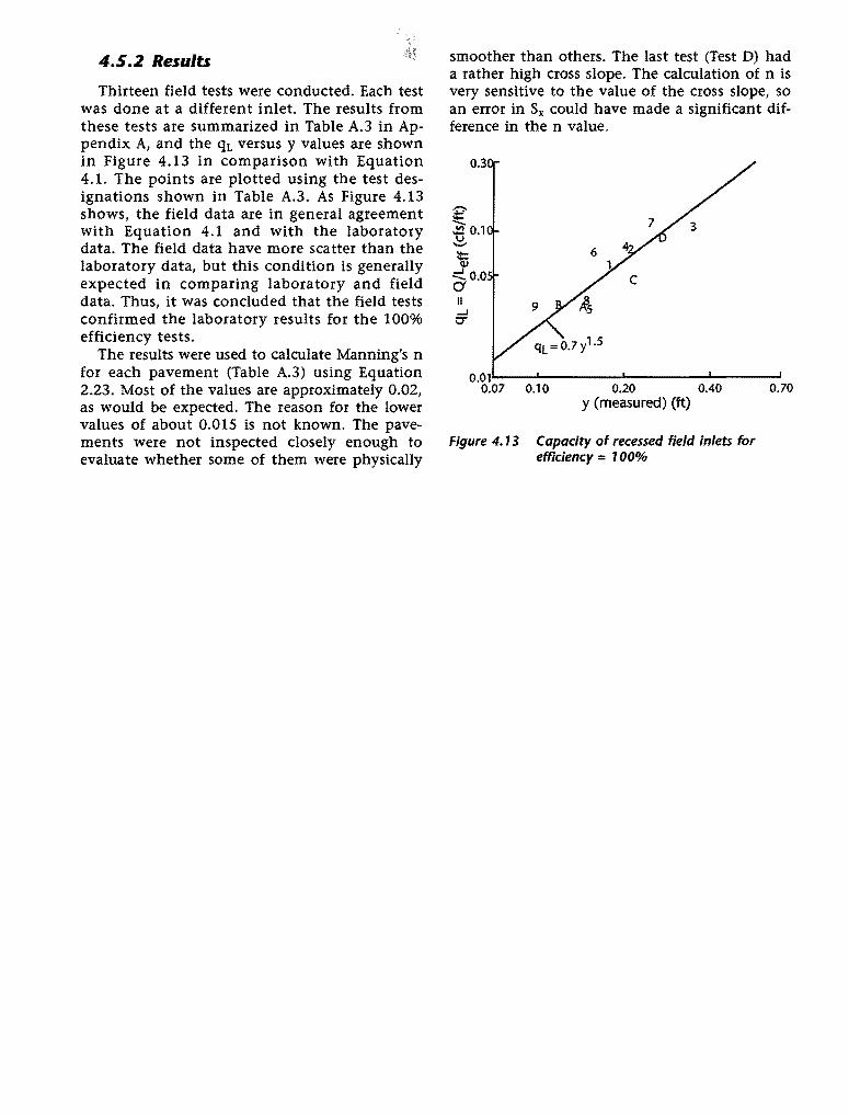
4.5.2 Results

Thirteen field tests were conducted. Each test was done at a different inlet. The results from these tests are summarized in Table A.3 in Ap­pendix A, and the qL versus y values are shown in Figure 4.13 in comparison with Equation 4.1. The points are plotted using the test des­ignations shown in Table A.3. As Figure 4.13 shows, the field data are in general agreement with Equation 4.1 and with the laboratory data. The field data have more scatter than the laboratory data, but this condition is generally expected in comparing laboratory and field data. Thus, it was concluded that the field tests confirmed the laboratory results for the 100% efficiency tests.

The results were used to calculate Manning's n for each pavement (Table A.3) using Equation 2.23. Most of the values are approximately 0.02, as would be expected. The reason for the lower values of about 0.015 is not known. The pave­ments were not inspected closely enough to evaluate whether some of them were physically

smoother than others. The last test (Test D) had a rather high cross slope. The calculation of n is very sensitive to the value of the cross slope, so an error in Sx could have made a significant dif­ference in the n value.

0.3

g '5 0.1 -~

...J 00.0 II ...J 0"'

0.011..---'-----...L-------JL..-..----1 0.07 0.10 0.20 0.40

y (measured) (ft)

Figure 4.13 Capacity of recessed field inlets for efficiency = 100%

0.70

30

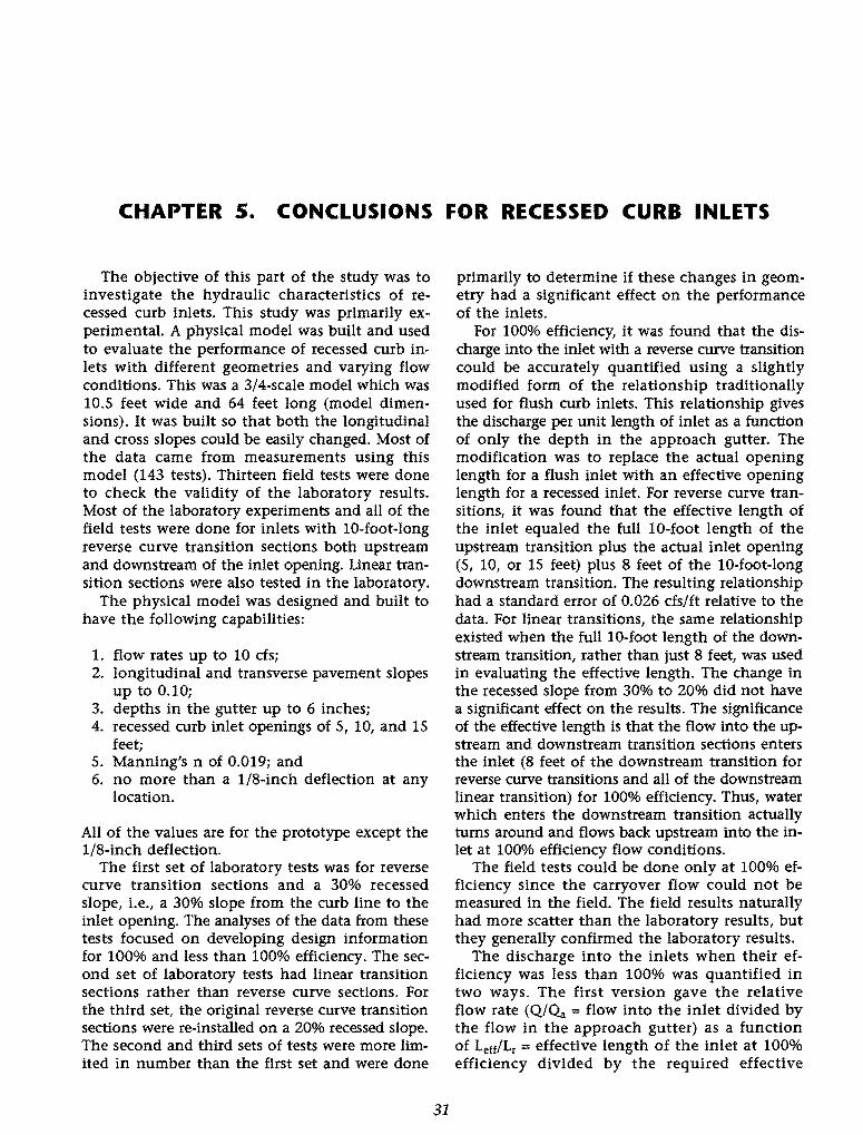
CHAPTER 5. CONCLUSIONS FOR RECESSED CURB INLETS

The objective of this part of the study was to investigate the hydraulic characteristics of re­cessed curb inlets. This study was primarily ex­perimental. A physical model was built and used to evaluate the performance of recessed curb in­lets with different geometries and varying flow conditions. This was a 3/4-scale model which was 10.5 feet wide and 64 feet long (model dimen­sions). It was built so that both the longitudinal and cross slopes could be easily changed. Most of the data came from measurements using this model (143 tests). Thirteen field tests were done to check the validity of the laboratory results. Most of the laboratory experiments and all of the field tests were done for inlets with 10-foot-long reverse curve transition sections both upstream and downstream of the inlet opening. Linear tran­sition sections were also tested in the laboratory.

The physical model was designed and built to have the following capabilities:

1. flow rates up to 10 ds; 2. longitudinal and transverse pavement slopes

up to 0.10; 3. depths in the gutter up to 6 inches; 4. recessed curb inlet openings of 5, 10, and 15

feet; 5. Manning's n of 0.019; and 6. no more than a 1/8-inch deflection at any

location.

All of the values are for the prototype except the 1/8-inch deflection.

The first set of laboratory tests was for reverse curve transition sections and a 30% recessed slope, i.e., a 30% slope from the curb line to the inlet opening. The analyses of the data from these tests focused on developing design information for 100% and less than 100% efficiency. The sec­ond set of laboratory tests had linear transition sections rather than reverse curve sections. For the third set, the original reverse curve transition sections were re-installed on a 20o/o recessed slope. The second and third sets of tests were more lim­ited in number than the first set and were done

31

primarily to determine if these changes in geom­etry had a significant effect on the performance of the inlets.

For 100% efficiency, it was found that the dis­charge into the inlet with a reverse curve transition could be accurately quantified using a slightly modified form of the relationship traditionally used for flush curb inlets. This relationship gives the discharge per unit length of inlet as a function of only the depth in the approach gutter. The modification was to replace the actual opening length for a flush inlet with an effective opening length for a recessed inlet. For reverse curve tran­sitions, it was found that the effective length of the inlet equaled the full 10-foot length of the upstream transition plus the actual inlet opening (5, 10, or 15 feet) plus 8 feet of the 10-foot-long downstream transition. The resulting relationship had a standard error of 0.026 cfs/ft relative to the data. For linear transitions, the same relationship existed when the full 10-foot length of the down­stream transition, rather than just 8 feet, was used in evaluating the effective length. The change in the recessed slope from 30% to 20% did not have a significant effect on the results. The significance of the effective length is that the flow into the up­stream and downstream transition sections enters the inlet (8 feet of the downstream transition for reverse curve transitions and all of the downstream linear transition) for 100% efficiency. Thus, water which enters the downstream transition actually turns around and flows back upstream into the in­let at 100% efficiency flow conditions.

The field tests could be done only at 100% ef­ficiency since the carryover flow could not be measured in the field. The field results naturally had more scatter than the laboratory results, but they generally confirmed the laboratory results.

The discharge into the inlets when their ef­ficiency was less than 100% was quantified in two ways. The first version gave the relative flow rate (Q/Oa = flow into the inlet divided by the flow in the approach gutter) as a function of Lett!Lr =effective length of the inlet at 100% efficiency divided by the required effective

length to capture all of the gutter flow. The standard error of the Q/Oa data relative to the equation which defined this relationship was 0.087. Due to the scatter of the data when ana­lyzed in terms of these variables, a second ap­proach was used. The data were replotted in terms of Q/Lett = the flow into the inlet divided by the inlet's effective length (33, 28, or 23 feet for reverse curve transitions) as a function of Oa/Lr = the flow rate in the approach gutter divided by the effective length required to cap­ture the entire flow. This type of plotting re­vealed a slight segregation of the data by inlet length and Froude number of the approach flow. Many types of correlations were tried to account for the effects of these additional vari­ables. The best relationship did provide an im­proved correlation, but the resulting equation was so complicated that it sometimes predicted

32

negative flows into the inlet for conditions out­side the range of conditions tested in the labo­ratory. Thus, it was recommended that the re­lationship between Q/Oa and LettiLr be used rather than the one between Q/Letf and Oa/Lr.

The results for less than 100% efficiency with a linear transition and with a 20% recessed slope were essentially unchanged from the original data set.

When recessed inlets capture less than 100% of the approach gutter flow, they are relatively less efficient than when they capture 100%. At less than 100% capture, some of the flow which en­ters the downstream transition section has enough momentum to flow back up the recessed slope and into the downstream gutter rather than flowing into the inlet. This effect was included in the predictive relationship which was developed for less than 100% efficiency.

PART II - BRIDGE DECK DRAINS

CHAPTER 6.

The drainage facilities installed in a bridge are important for ensuring that traffic remains pos­sible and safe during and after precipitation events. The storm water that falls on a bridge deck must be drained rapidly and efficiently in order to prevent its accumulation. At the same time, drains should not represent an obstacle to traffic, and they should be positioned in a way consistent with the bridge structure and geometry.

One of the objectives of this project was to gain an improved understanding of the hydraulics of three different types of bridge deck drains used in Texas and to produce design information for these drains. There were no previous studies of perfor­mance and efficiency for these particular drains. One drain was a rectangular scupper drain, which is basically a small opening in the bridge deck. The other two consisted of a grate installed on the bridge deck, followed by an inlet box and a piping system that drains the water through the bridge structure. Because of the lack of experimental data for these particular drains, they were previously being designed without adequate information.

The hydraulic characteristics of the drains, in­cluding the effects that the inlet boxes and drain pipes could have on their behavior, were studied using a hydraulic laboratory model. Experimental data on the capacity of the drains were obtained for different longitudinal and cross slopes of the simulated bridge deck for flow rates up to 3 cfs.

INTRODUCTION

33

The capacity and performance of on-grade grate inlets used for street drainage have been studied before. Currently, the Federal Highway Administration uses the manual "Drainage of Highway Pavements," Hydraulic Engineering Circular No. 12, by Johnson and Chang (1984) for the design and analysis of grate inlets. That publication has methods for analyzing seven different grate inlets. Because those design charts and methodologies are meant primarily for street drains, their applicability to the de­sign of bridge drains is limited. The reason is that bridge grates are followed by an inlet box and a piping system that are significantly differ­ent in dimension and geometry from inlet boxes and subsequent sewer pipes for street drains. The back-pressure effect that bridge inlet boxes and drain pipes can have on the capacity of the bridge grate inlets is what makes the methodol­ogy for street inlets not fully applicable for bridge deck drains. Johnson and Chang (1984) also presented design information for a circular 4-inch scupper drain. It is not clear from the publication whether the design information for these drains was based solely on calculations or on data. For this reason, and since the 4-inch­by-6-inch scupper drain, which is sometimes used, has almost twice the area of a 4-inch cir­cular drain, these rectangular scuppers were in­cluded in the experimental program.

1 1 1 1 1 1 1 1 1 1 1 1 1 1 1 1 1 1 1 1 1 1 1 1

34

1 1 1 1 1 1 1 1 1 1 1 1 1 1 1 1 1 1 1 1 1 1 1 1 1 1

CHAPTER 7. EXPERIMENTS AND RESULTS

7.1 ·rHE PHYSICAL MODEL

Experimental testing of the three bridge drains was done with the same model used for the ex­periments for recessed curb inlets discussed in Part I of this report. The model represented one traffic lane on a bridge deck. Even though the model was used as a 3/4-scale model for the study of recessed curb inlets, it was used as a full-scale model for the study of two of the bridge drains because of the lower flow rates involved and the smaller size of the drains. For the bridge drains, the cross slope was obtained by tilting the model roadway surface downward toward the left since these drains were on the left side of the model (Figure C.11) while it was tilted toward the right for the recessed curb inlets. In hydraulics, the normal convention is to define left and right looking in the direction of flow. Each of the drains was located approximately 40 feet down­stream of the head box.

7.2 MEASUREMENTS

The flow measurement devices were the same as those used for the tests with the recessed curb inlets (Section 3.6). The inflows to the model were small enough that all of the flow could be ob­tained with only one pump (Figure 3.4), so only the north pump and the venturi meter were used for obtaining and measuring the inflows. Each time that the venturi meter and the weirs were recalibrated, the results were within 1 o/o to 2% of the original calibration.

For Drains 2 and 3 discussed below, the flow into the inlet was determined as the difference between the total flow rate and the carryover flow, as for the recessed curb inlets. However, for the scupper drain, the flow into the drain was so small that it was measured volumetrically. For these measurements, a 12-inch flexible hose was mounted beneath the scupper to divert the flow. The hose was mounted in a manner to allow free flow of the water into and through the scupper. Normally, the flow just passed through the hose

35

to the return system. When it was desired to measure the flow rate, the bottom end of the hose was pulled over a cylindrical tank which had a diameter of 6.5 feet and a height of 2 feet. A stop watch was used to measure the filling time, which was typically 1 to 2 minutes. The flow rate was determined from the initial and final depth read­ings and the filling time. After a measurement, the tank was emptied by siphoning.

The depths and ponded widths were measured as for the recessed curb inlets in an attempt to determine these values for uniform flow. However, gradually varied flow existed in some regions of the flow so that it was not always possible to measure these quantities for uniform flow. De­pending on the flow conditions, the gradually varied flow regions were of different lengths and in different locations. For supercritical flow, there was gradually varied flow immediately down­stream of the head box and immediately down­stream of the drain. For subcritical flow, gradually varied flow existed immediately upstream of the drain and before the downstream end of the model where there was a free overfall. All of this behavior is in accordance with the theory of free surface flow. Nevertheless, uniform flow was sometimes established in only short lengths of the model. The location of these regions for each test depended on the longitudinal slope, cross-slope and total flow rate. For this reason, even though the desire was to measure the uniform flow depth upstream of the drain and to measure the flow width (ponded width) for uniform flow, this was not always possible. The depths were measured, but the correlations which are given later between the flow rates into the drains and the depths were based on calculated uniform flow depths.

The normal depth (y) next to the curb for the gutter flow was calculated in each case using the modified Manning's formula for free surface flow in a triangular channel (Equation 2.23). When the measured flow depths were compared with the calculated normal depths for the ap­proach flow, it was found for subcritical flows that the measured depths were smaller than the

calculated flow depths, in accordance with the theory of gradually varied flow for subcritical flow since an M2 curve existed upstream of the drain. For supercritical flows, the measured depths and the calculated normal depths were essentially the same (±5%) since uniform flow existed upstream of the drains. For all of the tests, the calculated normal depths were used for the analysis instead of the measured depth.

7.3 DRAIN 1 (SCUPPER DRAIN)

7.3.1 Geometry and Description

The first bridge deck drain was a rectangular scupper drain, which is basically an opening in the bridge deck. The water enters the drain and goes immediately into a free fall. The scupper drain was located nearly flush with the edge of the bridge deck. The model was used as a full-scale model for the scupper drain. The interior dimensions of the scupper were 4 inches (normal to the direction of flow) by 6 inches (in the direction of flow). The vertical length of the drain was 1 foot. It was con­structed of 3/4-inch plexiglass. The top edge of the scupper was flush with the roadway surface.

7.3.2 Procedures

The procedures were as follows:

1. The model was set at the desired longitudi­nal and cross slopes.

2. A constant total flow rate was established into the upstream end of the model using the venturi meter to determine the flow rate.

3. The flow depth and the ponded width were measured upstream and downstream of the drain.

4. When the flow over the total-flow V-notch weir reached a steady condition, the head on the weir was measured.

5. The flow rate into the scupper drain was measured volumetrically, as described in Sec­tion 7.2.

For the scupper drain, 7 4 tests were conducted. The data are shown in Table B.1, Appendix B. The tests had longitudinal slopes of 0.001, 0.005, 0.01, 0.02, 0.04 and 0.06 and transverse slopes of 0.01, 0.02, 0.04, 0.06 and 0.08. The range of total flows (gutter flows) was from 0.03 cfs to 3 cfs.

7.3.3 Results

A graph of the calculated normal depth (y) next to the curb upstream of the drain versus the

36

flow rate (Q1) captured by the scupper drain is shown in Figure 7 .1. All of the data points ob­tained during the testing appear on the graph. They are plotted in groups according to the lon­gitudinal slope (S) for each case. Thus, each sym­bol in Figure 7.1 represents the data for all of the cross slopes which were tested for the indicated longitudinal slope. A visual inspection of Figure 7.1 reveals the following:

• Up to at least y = 0.10 feet (or Q1 = 0.16 cfs), there is essentially a linear relationship be­tween log(Q1) and log(y) for each value of S. The scatter about each line in the figure may be due to the effect of the cross slope (SJ.

• From y = 0.10 feet to 0.40 feet, this linear re­lationship is not present for all longitudinal slopes (S). A change in the slope of the data points (called a break point) for log(Q1) ver­sus log(y) for each S exists, with the break point occurring at smaller values of y or Qa for larger longitudinal slopes. That is, the change in slope of the data occurs for S = 0.06 for a certain value of y, then it occurs for S = 0.04 for a larger value of y, and so on. The right-hand end of each solid line in the figure is at the point where the break in the slope of the data points appears to occur.

• The range of flows used during the testing does not permit a definite evaluation of the characteristics of the relationship between Q1 and y for the data past the break point in the slope of the data (i.e., for the largest y val­ues for each longitudinal slope).

• In the transition region to the right of and above the break points in the slopes of the data, the curves for the different values of S cross. For the lines shown, the data for S = 0.06 are the lowest points on the graph, but it ap­pears that they would be the highest values if there were enough data to define the variations for larger depths and larger flow rates.

• Comparing Figure 7.1 with the similar graph presented by Johnson and Chang (1984) for the 4-inch circular scupper drain, it can be seen that the results are generally similar.

• For flow conditions below the break points, the slopes of the data points for each of the longitudinal roadway slopes are essential­ly the same.

For the smaller flow depths and for subcritical flow, the flow into the scupper drain behaves as flow over a weir along each of the four sides. For supercritical flow, the same thing occurs, except that the water does not flow into the drain from the downstream side. At a certain flow depth, the

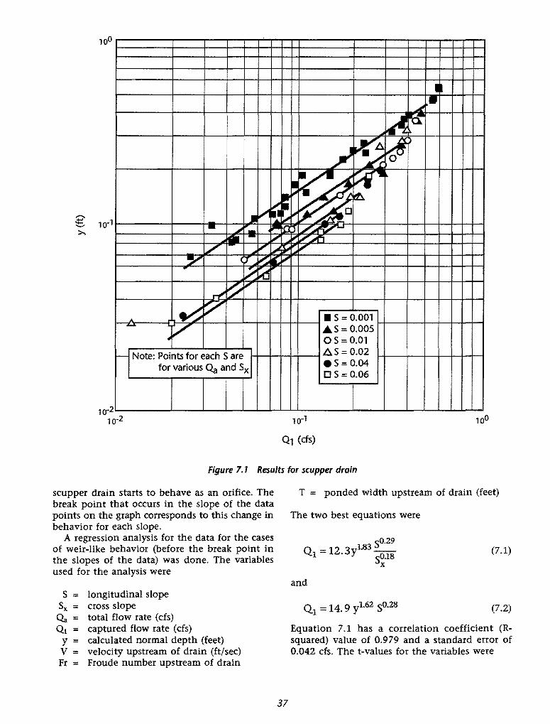
'iHt I

ff I I

.JI •• ~ ~ ;t..

f ~.6 ~ ~) 0

~~ ~ ~ = ~~

~ ~ ..1 ~ - __,

::! Iii'"" to J /~V"""'

1411 ~ ~ ~v~ v ~ ~ ~ ~...~~"' I ..,., f)' ~ lit v ~ w

~ I" ,...,

~ v A • s = 0.001 ...... 4v .AS= 0.005

0 s = 0.01

1-- Note: Points for each S are .65 = 0.02

for various ~ and Sx es = o.o4 CJ s = 0.06

Q1 (ds)

Figure 7.1 Results for scupper drain

scupper drain starts to behave as an orifice. The break point that occurs in the slope of the data points on the graph corresponds to this change in behavior for each slope.

A regression analysis for the data for the cases of weir-like behavior (before the break point in the slopes of the data) was done. The variables used for the analysis were

S = longitudinal slope Sx = cross slope aa = total flow rate (cfs) Q1 = captured flow rate (cfs)

y = calculated normal depth (feet) V = velocity upstream of drain (ft/sec) Fr = Froude number upstream of drain

37

T = ponded width upstream of drain (feet)

The two best equations were

(7.1)

and

(7.2)

Equation 7.1 has a correlation coefficient (R­squared) value of 0.979 and a standard error of 0.042 cfs. The t-values for the variables were

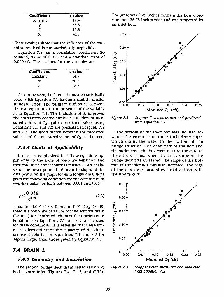
Coefficient t-value constant 19.4

y 35.8 5 27.3 Sx -6.5

These t-values show that the influence of the vari­ables involved is not statistically negligible.

Equation 7.2 has a correlation coefficient (R­squared) value of 0.955 and a standard error of 0.060 cfs. The t-values for the variables are

Coefficient constant

y s

t-value 14.9 28.3 18.6

As can be seen, both equations are statistically good, with Equation 7.1 having a slightly smaller standard error. The primary difference between the two equations is the presence of the variable Sx in Equation 7.1. The inclusion of Sx improves the correlation coefficient by 2.5%. Plots of mea­sured values of Q1 against predicted values using Equations 7.1 and 7.2 are presented in Figures 7.2 and 7.3. The good match between the predicted values and the measured values of Q 1 can be seen.

7.3.4 Limits of Applicability

It must be emphasized that these equations ap­ply only to the zone of weir-like behavior, and therefore their applicability is restricted. An analy­sis of the break points that occur in slopes of the data points on the graph for each longitudinal slope gives the following condition for the occurrence of weir-like behavior for S between 0.001 and 0.06:

< 0.034 Y- so39 (7.3)

Thus, for 0.001 ::;; S ::;; 0.06 and 0.01 ::;; Sx ::;; 0.08, there is a weir-like behavior for the scupper drain (Drain 1) for depths which meet the restriction in Equation 7.3; Equations 7.1 and 7.2 can be used for these conditions. It is essential that these lim­its be observed since the capacity of the drain decreases relative to Equations 7.1 and 7.2 for depths larger than those given by Equation 7.3.

7.4 DRAIN 2

7.4. 1 Geometry and Description

The second bridge deck drain tested (Drain 2) had a grate inlet (Figures 7.4, C.12, and C.13).

38

The grate was 9.25 inches long (in the flow direc­tion) and 36.75 inches wide and was supported by an inlet box.

-~ ~ .... 0.15

Cf "'C 2:l :5 0.10

~ Q..

0.05

tl

0.00 ~--.L.---.L..--__..JL---__JL-----1 0.00 0.05 0.10 0.15 0.20 0.25

Measured Q1 (cfs)

Figure 7.2 Scupper flows, measured and predicted from Equation 7.1

The bottom of the inlet box was inclined to­wards the entrance to the 6-inch drain pipe, which drains the water to the bottom of the bridge structure. The deep part of the box and the outlet from the box were next to the curb in these tests. Thus, when the cross slope of the bridge deck was increased, the slope of the bot­tom of the inlet box was also increased. The edge of the drain was located essentially flush with the bridge curb.

0.25

0.20 -:9, .... 0.15

Cf 1:1 "'C 2:l u 0.10 'i5 (!) ....

Q..

0.05

0.05 0.10 0.15 0.20 0.25

Measured Q1 (ds)

Figure 7.3 Scupper flows, measured and predicted from Equation 7.2

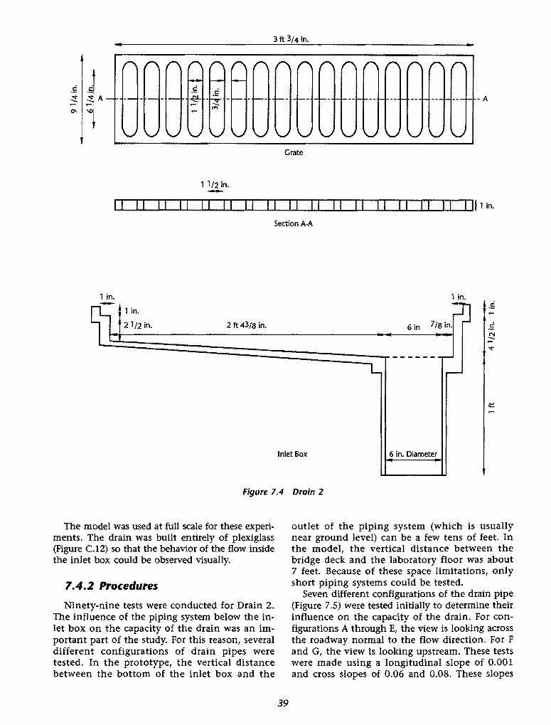
3ft 3/4 in.

A ·A

Grate

1 1/2 in. -I I I I II I I I I I I I I I I I I I I I I I I I I II I I I I I H lin.

Section A-A

1 in. 1 in.

- i 1 in. .5

2 1/2 in. 2 ft43/8 in. 6in .5 N -... '-==============::-r------

Inlet Box 6 in. Diameter

Figure 7.4 Drain 2

The model was used at full scale for these experi­ments. The drain was built entirely of plexiglass (Figure C.12) so that the behavior of the flow inside the inlet box could be observed visually.

7.4.2 Procedures

Ninety-nine tests were conducted for Drain 2. The influence of the piping system below the in­let box on the capacity of the drain was an im­portant part of the study. For this reason, several different configurations of drain pipes were tested. In the prototype, the vertical distance between the bottom of the inlet box and the

39

outlet of the piping system (which is usually near ground level) can be a few tens of feet. In the model, the vertical distance between the bridge deck and the laboratory floor was about 7 feet. Because of these space limitations, only short piping systems could be tested.

Seven different configurations of the drain pipe (Figure 7.5) were tested initially to determine their influence on the capacity of the drain. For con­figurations A through E, the view is looking across the roadway normal to the flow direction. For F and G, the view is looking upstream. These tests were made using a longitudinal slope of 0.001 and cross slopes of 0.06 and 0.08. These slopes

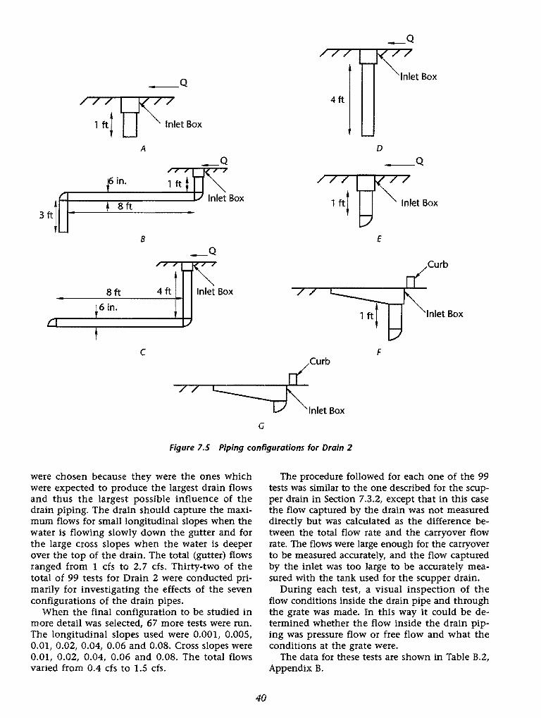
__ Q

__ Q Inlet Box

/77 4ft

D

in.

• 8ft Inlet Box

B E

,, , ~ ~

Curb

8ft 4ft Inlet Box

t6 in. Inlet Box lJ

t C F

Curb

77~ Inlet Box

G

Figure 7.5 Piping configurations for Drain 2

were chosen because they were the ones which were expected to produce the largest drain flows and thus the largest possible influence of the drain piping. The drain should capture the maxi­mum flows for small longitudinal slopes when the water is flowing slowly down the gutter and for the large cross slopes when the water is deeper over the top of the drain. The total (gutter) flows ranged from 1 cfs to 2. 7 cfs. Thirty-two of the total of 99 tests for Drain 2 were conducted pri­marily for investigating the effects of the seven configurations of the drain pipes.

When the final configuration to be studied in more detail was selected, 67 more tests were run. The longitudinal slopes used were 0.001, 0.005, 0.01, 0.02, 0.04, 0.06 and 0.08. Cross slopes were 0.01, 0.02, 0.04, 0.06 and 0.08. The total flows varied from 0.4 cfs to 1.5 cfs.

40

The procedure followed for each one of the 99 tests was similar to the one described for the scup­per drain in Section 7 .3.2, except that in this case the flow captured by the drain was not measured directly but was calculated as the difference be­tween the total flow rate and the carryover flow rate. The flows were large enough for the carryover to be measured accurately, and the flow captured by the inlet was too large to be accurately mea­sured with the tank used for the scupper drain.

During each test, a visual inspection of the flow conditions inside the drain pipe and through the grate was made. In this way it could be de­termined whether the flow inside the drain pip­ing was pressure flow or free flow and what the conditions at the grate were.

The data for these tests are shown in Table B.2, Appendix B.

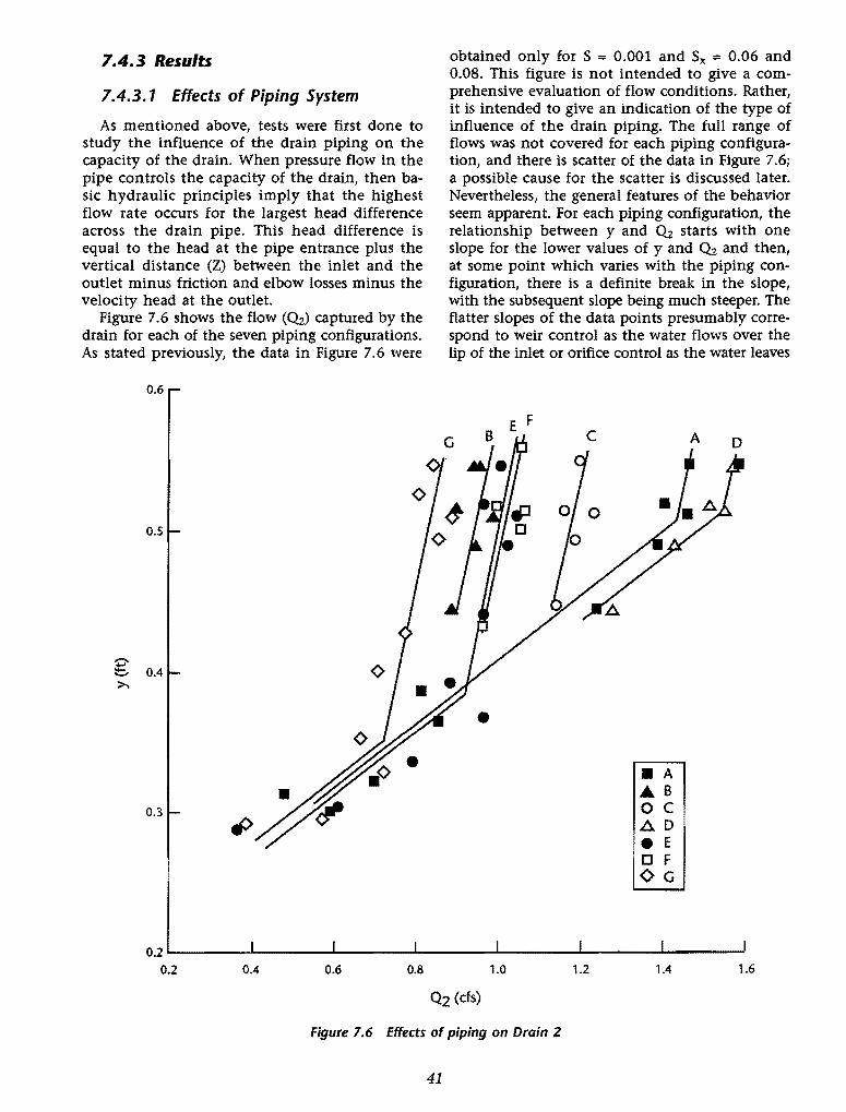
7.4.3 Results

7.4.3.1 Effects of Piping System

As mentioned above, tests were first done to study the influence of the drain piping on the capacity of the drain. When pressure flow in the pipe controls the capacity of the drain, then ba­sic hydraulic principles imply that the highest flow rate occurs for the largest head difference across the drain pipe. This head difference is equal to the head at the pipe entrance plus the vertical distance (Z) between the inlet and the outlet minus friction and elbow losses minus the velocity head at the outlet.

Figure 7.6 shows the flow (Qz) captured by the drain for each of the seven piping configurations. As stated previously, the data in Figure 7.6 were

0.6

0.5

Z' \::!::.. 0.4 >.

0.3

tl>

obtained only for S = 0.001 and Sx = 0.06 and 0.08. This figure is not intended to give a com­prehensive evaluation of flow conditions. Rather, it is intended to give an indication of the type of influence of the drain piping. The full range of flows was not covered for each piping configura­tion, and there is scatter of the data in Figure 7.6; a possible cause for the scatter is discussed later. Nevertheless, the general features of the behavior seem apparent. For each piping configuration, the relationship between y and Qz starts with one slope for the lower values of y and Qz and then, at some point which varies with the piping con­figuration, there is a definite break in the slope, with the subsequent slope being much steeper. The flatter slopes of the data points presumably corre­spond to weir control as the water flows over the lip of the inlet or orifice control as the water leaves

F B E

•

c A

• A ..A.B 0 c .6.0 e E IJ F ¢G

0.2~------~------~--------._------~------~--------._------~ 0.2 0.4 0.6 0.8 1.0 1.2 1.4 1.6

Figure 7.6 Effects of piping on Drain 2

41

the inlet box and enters the piping system. The steeper slopes correspond to back-pressure effects from the piping system controlling the flow. For the regions of the steeper slopes in Figure 7.6, the pipe was flowing full. Using the letter designations of the drain configurations shown in Figure 7.5 to identify the flow for the different configurations, an inspection of Figure 7.6 shows for the regions of back-pressure control that

1. Qz(A) < Qz(D), which is in accordance with hydraulic theory. The vertical distance (Z) between inlet and outlet is larger in D than in A, so that there is a larger head difference across the pipe, and there are no elbows in either one to affect the head losses in the piping system.

2. Qz(B) < Qz(C) < Qz(D), with significant differ­ences for the three cases even though the ver­tical distance between the inlet and outlet is the same for all three cases. Configuration B is shown in Figure C.l4. The fact that Qz(D) is the largest is in accordance with hydraulics theory since it has no elbows to cause losses and since it has the shortest pipe. It is curi­ous that Qz(C) is larger than Qz(B), despite the fact that both configurations have the same pipe length, the same number of elbows, and the same Z. The essential difference between B and C is that the first elbow is closer to the inlet for B than for C.

3. Qz(B) < Qz(E), but the difference is small. It is somewhat surprising that Qz(B) is not sig­nificantly larger than Qz(E), since B appears to have a significantly larger head difference across the pipe than E due to the extra 3-foot drop for B. The additional head loss for B due to the extra pipe length and the extra elbow is only about 0.6 feet. The essential feature which is the same for B and E is the distance from the inlet to the first elbow.

4. Qz(E) = Qz(F), with the difference in the pipe configurations for E and F being only the direction that the elbow is turned.

5. Qz(G) < Qz(F), with the vertical distance to the elbow for G (Figure C.12) being smaller than for F. It is difficult to know whether the reduction in flow for G is due to the elbow being closer to the inlet box or due to the reduction in head difference across the pipe with the outlet being 1 foot higher for G.

6. The flow differences for the various piping configurations are much greater for back-pres­sure control than for weir (or orifice) control.

From these observations, it appears that the dis­tance to the first elbow has a very strong influence

42

on the amount of flow captured by the drain when back-pressure conditions exist, with less flow being captured by the inlet for smaller distances to the first elbow. The hydraulic reasons for this effect are not clear, but this distance appears to be very im­portant for establishing the flow into the piping system, especially when the distance between in­let box and elbow is small. Based on these results, it was decided to conduct a complete set of tests for configuration G, since this configuration had the smallest capacity.

The results give good confirmation that con­figuration G has the smallest capacity of the configurations tested in the laboratory. Neverthe­less, it is possible that the behavior would be dif­ferent if the head difference across the drain pip­ing were on the order of 15 feet to 20, as it might be for a bridge with the piping outlet near ground leveL

7.4.3.2 Results for Low Flow Conditions

The discussion in Section 7.4.3.1 above relates primarily to conditions when the piping system causes a back-pressure effect which controls the capacity of the inlet. Even for the worst case (con­figuration G), there is no back-pressure effect up to a flow of about 0.7 cfs. For the other configu­rations, higher flows can be captured with no back-pressure effects. Thus, for the most common ranges of flows for these bridge drains, it can be anticipated that low flow conditions (no back­pressure effects) will prevail. For contrast with these intercepted flows for Drain 2, the maximum flow shown by Johnson and Chang (1984) on the design graph for a 4-inch circular scupper drain is only 0.17 cfs and low flow conditions are shown to stop at about 0.07 cfs. For the 4-inch­by-6-inch rectangular scupper discussed in Section 7.3, low flow conditions existed up to at least 0.2 cfs (Figure 7.1 and Equation 7 .3).

The remainder of the experimental program for Drain 2 was directed toward determining the ca­pacity for low flow conditions for a range of lon­gitudinal and cross slopes. For these additional tests, the maximum gutter flow rate was 2.6 cfs, and the maximum drain flow rate was 0.8 cfs (for all but three of the tests). The gutter flow rates were selected, in combination with the slopes, to give drain flows which would be in the low flow regime with no effects of back pressure and to cover the expected range of gutter flows.

The results of the additional tests for configu­ration G plus the low-flow tests for all of the pre­vious piping configurations are shown in Figure 7. 7. There is a general segregation of the data according to longitudinal slope (S), but there is

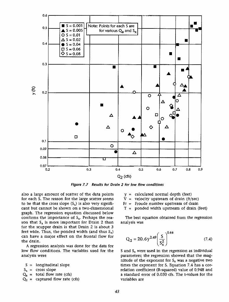
0.6

• • s = 0.001 ._ Note: Points for each S are • -.&S = 0.005 0.5

for various C4J and Sx ·-0 s = 0.01 AS= 0.02 • • s = 0.04 -0.4

[] s = 0.06 <> s = 0.08 • •

• • .~ 0.3

... <»..

... ... ( A.& 0.2

0.1

0.09

0.08

0.07 0.2

• []

• A

A

0

u

0.3

n_

0

0

..... 0 • <>

... <> .a.

• A

0.4 0.5

... All. • A

A 0

~ A [] <i • [~0

A

•

0.6 0.7 0.8 0.9

Figure 7.7 Results for Drain 2 for low flow conditions

also a large amount of scatter of the data points for each S. The reason for the large scatter seems to be that the cross slope (Sx) is also very signifi­cant but cannot be shown on a two-dimensional graph. The regression equation discussed below confirms the importance of Sx. Perhaps the rea­son that Sx is more important for Drain 2 than for the scupper drain is that Drain 2 is about 3 feet wide. Thus, the ponded width (and thus Sx) can have a major effect on the frontal flow for the drain.

A regression analysis was done for the data for low flow conditions. The variables used for the analysis were

S longitudinal slope Sx = cross slope ~ = total flow rate (cfs) Qz = captured flow rate (cfs)

43

y = calculated normal depth (feet) V = velocity upstream of drain (ft/sec) Fr = Froude number upstream of drain T = ponded width upstream of drain (feet)

The best equation obtained from the regression analysis was

( ]

0.44

Qz = 20.6y2.49 ~ (7.4)

S and Sx were used in the regression as individual parameters; the regression showed that the mag­nitude of the exponent for Sx was a negative two times the exponent for S. Equation 7.4 has a cor­relation coefficient (R-squared) value of 0.948 and a standard error of 0.030 cfs. The t-values for the variables are

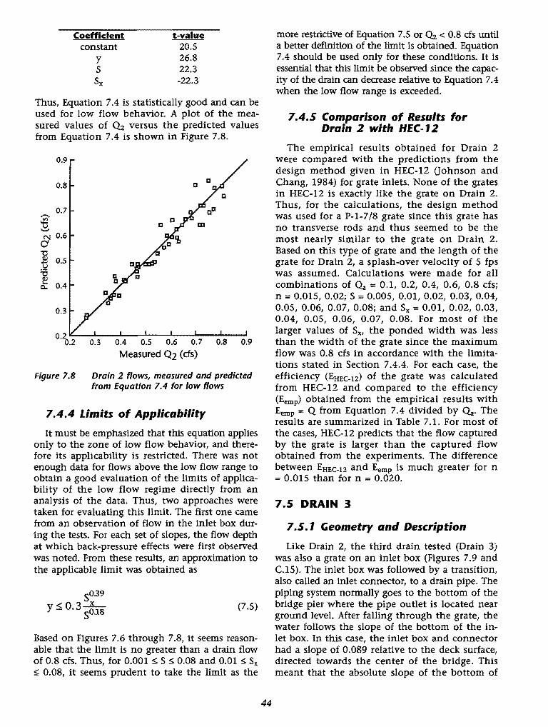
Coefficient t·value constant 20.5

y 26.8 s 22.3 Sx ·22.3

Thus, Equation 7.4 is statistically good and can be used for low flow behavior. A plot of the mea­sured values of (b versus the predicted values from Equation 7.4 is shown in Figure 7.8.

0.9

0.8 1:1

0.7 ,.._, ~ u '-' N 0.6

Cf "0 (!) 0.5 ..... u :0 (!) ... 0.4 0..

0.3

0.2 IC....-..L.--...1----'----L.---L.----'----' 0.2 0.3 0.4 0.5 0.6 0.7 0.8 0.9

Measured Q2 (ds)

Figure 7.8 Drain 2 flows, measured and predicted from Equation 7.4 for low flows

7.4.4 Limits of Applicability

It must be emphasized that this equation applies only to the zone of low flow behavior, and there­fore its applicability is restricted. There was not enough data for flows above the low flow range to obtain a good evaluation of the limits of applica· bility of the low flow regime directly from an analysis of the data. Thus, two approaches were taken for evaluating this limit. The first one came from an observation of flow in the inlet box dur­ing the tests. For each set of slopes, the flow depth at which back·pressure effects were first observed was noted. From these results, an approximation to the applicable limit was obtained as

so39 Y :::; o. 3 s~-ts (7.5)

Based on Figures 7.6 through 7 .8, it seems reason­able that the limit is no greater than a drain flow of 0.8 cfs. Thus, for 0.001 s S s 0.08 and 0.01 s Sx s 0.08, it seems prudent to take the limit as the

44

more restrictive of Equation 7.5 or Qz < 0.8 cfs until a better definition of the limit is obtained. Equation 7.4 should be used only for these conditions. It is essential that this limit be observed since the capac­ity of the drain can decrease relative to Equation 7.4 when the low flow range is exceeded.

7.4.5 Comparison of Results for Drain 2 with HEC- J 2

The empirical results obtained for Drain 2 were compared with the predictions from the design method given in HEC-12 Oohnson and Chang, 1984) for grate inlets. None of the grates in HEC-12 is exactly like the grate on Drain 2. Thus, for the calculations, the design method was used for a P-1-7/8 grate since this grate has no transverse rods and thus seemed to be the most nearly similar to the grate on Drain 2. Based on this type of grate and the length of the grate for Drain 2, a splash-over velocity of 5 fps was assumed. Calculations were made for all combinations of Oa = 0.1, 0.2, 0.4, 0.6, 0.8 cfs; n = 0.015, 0.02; S = 0.005, 0.01, 0.02, 0.03, 0.04, 0.05, 0.06, 0.07, 0.08; and Sx = 0.01, 0.02, 0.03, 0.04, 0.05, 0.06, 0.07, 0.08. For most of the larger values of Sx, the ponded width was less than the width of the grate since the maximum flow was 0.8 cfs in accordance with the limita· tions stated in Section 7 .4.4. For each case, the efficiency (EHEc-d of the grate was calculated from HEC-12 and compared to the efficiency (Eemp) obtained from the empirical results with Eemp = Q from Equation 7.4 divided by Oa· The results are summarized in Table 7.1. For most of the cases, HEC-12 predicts that the flow captured by the grate is larger than the captured flow obtained from the experiments. The difference between EHEc-12 and Eemp is much greater for n = 0.015 than for n = 0.020.

7.5 DRAIN 3

7.5. J Geometry and Description

Like Drain 2, the third drain tested (Drain 3) was also a grate on an inlet box (Figures 7.9 and C.15). The inlet box was followed by a transition, also called an inlet connector, to a drain pipe. The piping system normally goes to the bottom of the bridge pier where the pipe outlet is located near ground level. After falling through the grate, the water follows the slope of the bottom of the in· let box. In this case, the inlet box and connector had a slope of 0.089 relative to the deck surface, directed towards the center of the bridge. This meant that the absolute slope of the bottom of

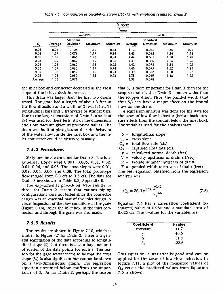
Table 7.1 Comparison of calculations from HEC-12 with empirical results for Drain 2

EHEC-12

Eemp

n=0.020 n=O.OlS

Standard Standard

_i_ Average Deviation Maximum Minimum Average Deviation Maximum Minimum

0.01 0.95 0.125 1.12 0.64 0.02 1.07 0.079 1.17 0.84 0.03 1.09 0.066 1.20 0.94 0.04 1.09 0.062 1.19 0.96 0.05 1.08 0.060 1.18 0.95 0.06 1.07 0.060 1.17 0.94 0.07 1.06 0.059 1.16 0.94 0.08 1.06 0.059 1.15 0.93

Average 1.06 0.071

the inlet box and connector decreased as the cross slope of the bridge deck increased.

This drain was larger than the first two drains tested. The grate had a length of about 3 feet in the flow direction and a width of 2 feet. It had 11 longitudinal bars and 5 transverse or stringer bars. Due to the larger dimensions of Drain 3, a scale of 3/4 was used for these tests. All of the dimensions and flow rates are given as prototype values. The drain was built of plexiglass so that the behavior of the water flow inside the inlet box and the in­let connector could be observed visually.

7.5.2 Procedures

Sixty-one tests were done for Drain 3. The lon­gitudinal slopes were 0.001, 0.005, 0.01, 0.02, 0.04, 0.06, and 0.08. The cross slopes were 0.01, 0.02, 0.04, 0.06, and 0.08. The total prototype flow ranged from 0.3 cfs to 3.5 cfs. The data for Drain 3 are shown in Table B.3, Appendix B.

The experimental procedures were similar to those for Drain 2 except that various piping configurations were not tested since the connector design was an essential part of the inlet design. A visual inspection of the flow conditions at the grate (Figure C.16), inside the inlet box, in the inlet con­nector, and through the grate was also made.

7.5. 3 Results

The results are shown in Figure 7.10, which is similar to Figure 7.7 for Drain 2. There is a gen­eral segregation of the data according to longitu­dinal slope (S), but there is also a large amount of scatter of the data points for each S. The rea­son for the large scatter seems to be that the cross slope (SJ is also significant but cannot be shown on a two-dimensional graph. The regression equation presented below confirms the impor­tance of Sx. As for Drain 2, perhaps the reason

45

1.13 0.072 1.50 090 1.43 0.092 1.56 1.16 1.44 0.085 1.58 1.28 1.43 0.080 1.56 1.26 1.42 0.078 1.54 1.25 1.40 0.075 1.52 1.23 1.39 0.072 1.50 1.22 1.38 0.069 1.48 1.22 1.38 0.078

that Sx is more important for Drain 3 than for the scupper drain is that Drain 3 is much wider than the scupper drain. Thus, the ponded width (and thus Sx) can have a major effect on the frontal flow for the drain.

A regression analysis was done for the data for the cases of low flow behavior (before back-pres­sure effects from the conduit below the inlet box). The variables used for the analysis were

S = longitudinal slope Sx = cross slope ~ = total flow rate (cfs) OJ = captured flow rate (cfs)

y = calculated normal depth (feet) V = velocity upstream of drain (ft/sec) Fr = Froude number upstream of drain T = ponded width upstream of drain (feet)

The best equation obtained from the regression analysis was

5o.4z Q3 = 26.Iyz.z6 so.66

X

(7.6)

Equation 7.6 has a correlation coefficient (R­squared) value of 0.984 and a standard error of 0.025 cfs. The t-values for the variables are

Coefficient constant

y s Sx

t-value 41.7 40.6 31.8 -22.6

This equation is statistically good and can be applied for the cases of low flow behavior. In Figure 7.11, a plot of the measured values of OJ versus the predicted values from Equation 7.6 is shown.

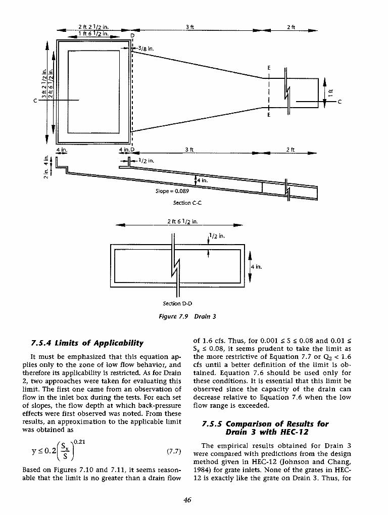
.5 .5 ~ N\0 -t=.t= M N

.,. 2ft21/2in. .,.. 1 ft 6 112 in . .,.

c --lH-IH--1--

4 in. -!t N

2ft ...

---+----C

E

2ft .. 4 in.

Slope == 0.089

Section C-C

2ft 6112 in.

tl/2 in.

t v I

Section D-D

Figure 7.9 Drain 3

7.S.4 Limits of Applicability

It must be emphasized that this equation ap­plies only to the zone of low flow behavior, and therefore its applicability is restricted. As for Drain 2, two approaches were taken for evaluating this limit. The first one came from an observation of flow in the inlet box during the tests. For each set of slopes, the flow depth at which back-pressure effects were first observed was noted. From these results, an approximation to the applicable limit was obtained as

(s )0.21

y ~ 0.2 ; (7.7)

Based on Figures 7.10 and 7.11, it seems reason­able that the limit is no greater than a drain flow

46

of 1.6 cfs. Thus, for 0.001 s S s 0.08 and 0.01 s Sx s 0.08, it seems prudent to take the limit as the more restrictive of Equation 7.7 or Qz. < 1.6 cfs until a better definition of the limit is ob­tained. Equation 7.6 should be used only for these conditions. It is essential that this limit be observed since the capacity of the drain can decrease relative to Equation 7.6 when the low flow range is exceeded.

7.S.S Comparison of Results for Drain 3 with HEC- I 2

The empirical results obtained for Drain 3 were compared with predictions from the design method given in HEC-12 (Johnson and Chang, 1984) for grate inlets. None of the grates in HEC-12 is exactly like the grate on Drain 3. Thus, for

Section E-E

3 ft

1 l

1 ft

2ft

1\

I 1/

~ 1 in. X 3/s in. 6 in. Space Center to Center

v Beanng Bars

3 112 in. X 1/2 in. 2-in. Space Center to Center

Section A-A I'RRFlff t3/s in.

)b U ~~earing Bars • • 4 . X 11 • X 1/. 31/2in.Xl/2in. L ln. 1 2 ln. 2 ln. 2-in. Space Center to Center

Figure 7.9 Drain 3 (continued)

the calculations, the design method was used for a P-1-7/8-4 grate since this grate seemed to be the most nearly similar to the grate on Drain 3. Based on this type of grate and the length of the grate for Drain 3, a splash-over velocity of 6.2 fps was assumed. Calculations were made for all combinations of <4 = 0.1, 0.2, 0.4, 0.6, 0.8 cfs; n = 0.015, 0.02; S = 0.005, 0.01, 0.02, 0.03, 0.04, 0.05, 0.06, 0.07, 0.08; and Sx = 0.01, 0.02, 0.03, 0.04, 0.05, 0.06, 0.07, 0.08. For each case, the efficiency (EHEc-d of the grate was calculated from HEC-12 and compared to the efficiency (Eemp) obtained from the empirical results with

47

Eemp = Q from Equation 7.6 divided by <4. Any conditions which violated the limits of appli­cability in Section 7.5.4 were eliminated. The results are summarized in Table 7 .2. For n = 0.020, except for Sx = 0.01, the averages of the calculated and measured results are very close to each other. However, as the standard deviation, maximum, and minimum show, some of the val­ues had as much as a 11 o/o difference from unity. For most of the cases with n = 0.015, HEC-12 predicts that the flow captured by the grate is much larger than the captured flow obtained from the experiments.

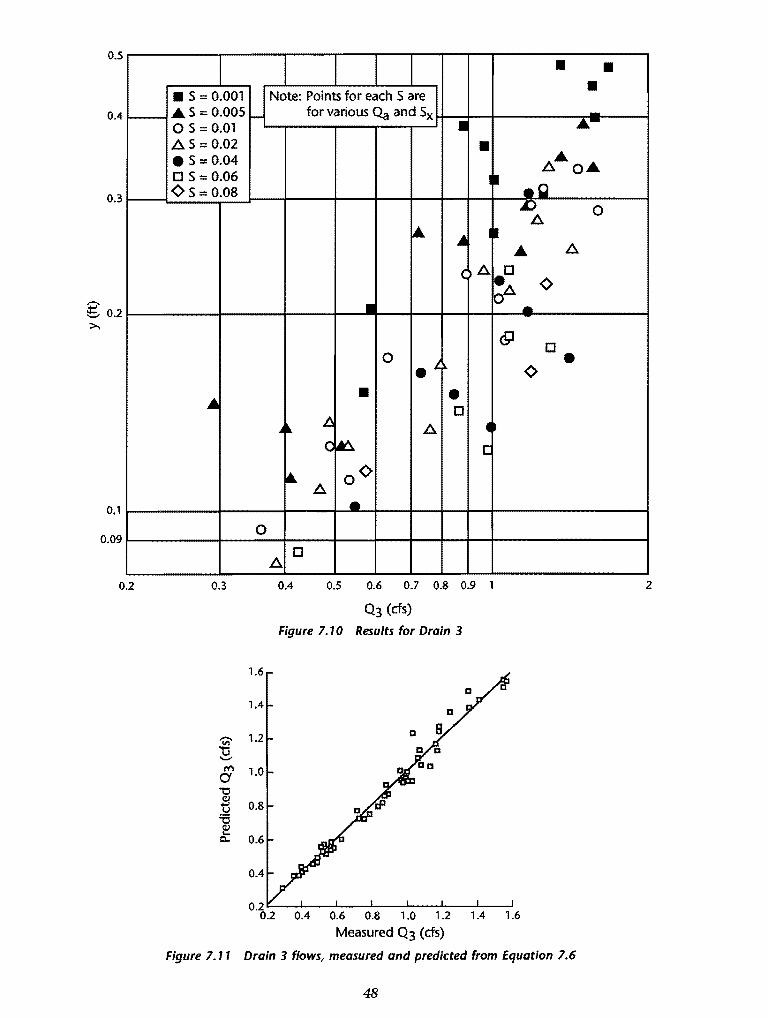
0.5 • • • s = 0.001 Note: Points for each S are • .&S =0.005 1- for various <la and Sx -0 s = 0.01 I ·-0.4

AS =0.02 • • 5=0.04 A•o• [J s = 0.06 • <> s- 0.08 .c

~ 0 A

lA ~ • • A

0.3

( A [J

~ <>

• -2 ........ 0.2 >-.

<9 [J 0

• i.~ • <>

... • • [J

.. ~ Jj

A 4 c ~ c

~ A

o<>

0.1 • 0.09

0

A [J

0.2 0.3 0.4 0.5 0.6 0.7 0.8 0.9 1 2

Q3 (ds)

Figure 7.10 Results for Drain 3

1.6

1.4

0.4 0.6 0.8 1.0 1.2 1.4 1.6

Measured Q3 (cfs)

Figure 7.11 Drain 3 flows, measured and predicted from Equation 7.6

48

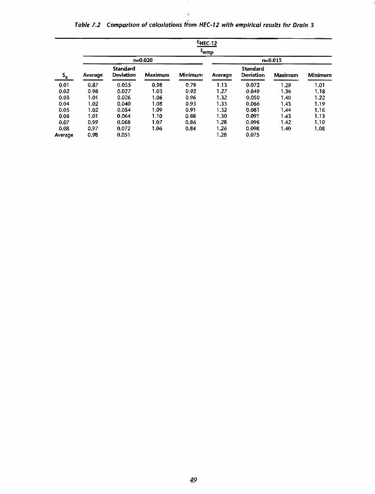
' Table 7.2 Comparison of calculations flom HEC-72 with empirical results for Drain 3

EHEC-12

Eemp

n=0.020 n=0.015

Standard Standard sx Average Deviation Maximum Minimum Average Deviation Maximum Minimum

0.01 0.87 0.055 0.98 0.79 1.13 0.072 1.29 1.01 0.02 0.98 0.027 1.03 0.92 1.27 0.049 1.36 1.18 0.03 1.01 0.026 1.06 0.96 1.32 0.050 1.40 1.22 0.04 1.02 0.040 1.08 0.93 1.33 0.066 1.43 1.19 0.05 1.02 0.054 1.09 0.91 1.32 0.081 1.44 1.16 0.06 1.01 0.064 1.10 0.88 1.30 0.091 1.43 1.13 0.07 0.99 0.068 1.07 0.86 1.28 0.096 1.42 1.10 0.08 0.97 0.072 1.06 0.84 1.26 0.098 1.40 1.08

Average 0.98 0.051 1.28 0.075

49

so

CHAPTER 8. CONCLUSIONS FOR BRIDGE DECK DRAINS

This part of the study was concerned with the capacity of three types of bridge deck drains. The ultimate objective was to obtain predictive equa­tions for the capacity of the drains, but a complementary objective was to gain an im­proved understanding of the hydraulics which control this capacity. To meet these objectives, experiments were conducted in a large laboratory facility constructed especially for this project. This facility represented one lane of a roadway and was built so that both the longitudinal and the cross slopes of the roadway could be easily changed. The surface of the roadway was covered with sand grains to produce a model Manning's n of 0.019. The details of the model are pre­sented in Part I of this report.

Drain 1 was a 4-inch-by-6-inch scupper drain while Drains 2 and 3 were different sizes and types of grated-inlets drains. The two smaller drains (Drain 1 and Drain 2, Figure 7.4) were tested at full scale. Drain 3 (Figure 7.9) was tested at 3/4 scale. Information was previously available for circular scuppers but not for rectangular ones. Likewise, some information was previously avail­able for grated inlets, but primarily for street drains which generally have larger inlet boxes and less restrictive piping systems following the boxes than is the case for bridge drains. That is, the previously available information on grated inlets is applicable primarily for situations where the inlet opening size and the grate itself normally control the capacity. Thus, for Drains 2 and 3, attention was given to investigating the effects of the inlets' boxes and the subsequent piping on the drain capacity. These drains were constructed of plexiglass so that the behavior of the flow in­side the inlet box and subsequent piping could be observed. For all three drains, empirical equations were obtained for predicting the capacity for the flow conditions most likely to be encountered on bridges. There generally is not a need to have predictive equations for the higher flow condi­tions, so these conditions were not tested exten­sive enough to obtain such equations.

51

For each drain, many tests (74 for Drain 1, 99 for Drain 2, and 61 for Drain 3) were conducted for a variety of longitudinal slopes (S), cross slopes (Sx), and flow rates (0a) upstream of the drains. The graphs showing the capacity of the drains as a function of the upstream uniform flow depth generally showed a change in behavior at some values of depth and flow. From the previously published results for drains and from observing the behavior of the flow during the testing, it could be concluded that the data trend for the smaller depths and the smaller flows corre­sponded to weir-like behavior for the flow enter­ing the inlets or possibly orifice control at the entrance to the drain piping for Drains 2 and 3. On the other hand, the behavior for larger depths and inlet flow rates corresponded to orifice con­trol for the scupper drain and to back-pressure effects for the other two drains which were fol­lowed by piping systems. For the scupper, the change in behavior had to correspond to chang­ing from weir to orifice flow since there is no piping below the scupper to create back-pressure effects. For the other two drains, the change in behavior presumably corresponded to back-pres­sure effects since visual observation of the flow in the plexiglass drain piping showed that the pip­ing was full when the second type of behavior was obtained. Since the back-pressure effects ex­isted primarily for flows beyond the normally expected range of flow on bridge decks, the test­ing program did not include enough flow condi­tions in this back-pressure range to obtain defini­tive predictive equations. Nevertheless, the testing did allow a reasonable determination of the limit of the range of low flow conditions. For each drain, predictive equations were obtained for the drain capacity for low flow and the limits of ap­plicability for low flow were also specified.

The type of results obtained for the 4-inch-by-6-inch scupper drain are generally comparable to those presented by Chang and Johnson (1984) for 4-inch circular scupper drains. In both types of scuppers, there is a clear difference in the trend

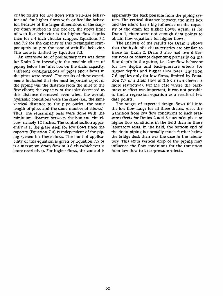
of the results for low flows with weir-like behav­ior and for higher flows with orifice-like behav­ior. Because of the larger dimensions of the scup­per drain studied in this project, the upper limit of weir-like behavior is for higher flow depths than for a 4-inch circular scupper. Equations 7.1 and 7.2 for the capacity of this rectangular scup­per apply only to the zone of weir-like behavior. This zone is limited by Equation 7.3.

An extensive set of preliminary tests was done for Drain 2 to investigate the possible effects of piping below the inlet box on the drain capacity. Different configurations of pipes and elbows in the pipes were tested. The results of these experi­ments indicated that the most important aspect of the piping was the distance from the inlet to the first elbow; the capacity of the inlet decreased as this distance decreased even when the overall hydraulic conditions were the same (i.e., the same vertical distance to the pipe outlet, the same length of pipe, and the same number of elbows). Thus, the remaining tests were done with the minimum distance between the box and the el­bow, namely 12 inches. The control section appar­ently is at the grate itself for low flows since the capacity (Equation 7.4) is independent of the pip­ing system for these flows. The limit of applica­bility of this equation is given by Equation 7.5 or is a maximum drain flow of 0.8 cfs (whichever is more restrictive). For higher flows, the control is

52

apparently the back pressure from the piping sys­tem. The vertical distance between the inlet box and the elbow has a big influence on the capac­ity of the drain for higher flows. Again, as for Drain 1, there were not enough data points to obtain flow equations for higher flows.

The analysis of the results for Drain 3 shows that the hydraulic characteristics are similar to those for Drain 2. Drain 3 also had two differ­ent types of behavior depending primarily on the flow depth in the gutter, i.e., low flow behavior for low depths and back-pressure effects for higher depths and higher flow rates. Equation 7.6 applies only for low flows, limited by Equa­tion 7.7 or a drain flow of 1.6 cfs (whichever is more restrictive). For the case where the back­pressure effect was important, it was not possible to find a regression equation as a result of few data points.

The ranges of expected design flows fell into the low flow range for all three drains. Also, the transition from low flow conditions to back pres­sure effects for Drains 2 and 3 may take place at higher flow conditions in the field than in these laboratory tests. In the field, the bottom end of the drain piping is normally much farther below the bridge deck than was the case in the labora­tory. This extra vertical drop of the piping may influence the flow conditions for the transition from low flow to back-pressure effects.

REFERENCES

Bauer, W. J., and D. C. Woo, "Hydraulic Design of Depressed Curb-Opening Inlets," Highway Research Record, No. 58, 1964, pp 61-80.

Bos, M. G., Discharge Measurement Structures, Delft Hydraulics Laboratory, Publication No. 161, Delft, The Netherlands, 1970, pp 168, 464.

Brater, E. F., and H. W. King, Handbook of Hydraulics, Sixth Edition, McGraw-Hill, New York, 1976, pp 2.85-2.86, 2.55-2.64.

Conner, N. W., "Design and Capacity of Gutter Inlets," Bulletin No. 30, North Carolina State College, Engineering Experiment Station (as cited by Izzard, 1950), 1945.

Corps of Engineers, "Airfield Drainage Structure Investigations," Hydraulic Laboratory Report No. 54, U.S. Army Corps of Engineers, St. Paul District Sub-Office (as cited by Izzard, 1950), 1949.

Davis, C. V., and K. E. Sorenson, Handbook of Applied Hydraulics, Third Edition, McGraw-Hill, New York, 1969, pp 2.25-2.27.

Forbes, H. J. C., "Capacity of Lateral Stormwater Inlets," The Civil Engineer in South Africa, Vol 18, No. 9, 1976, pp 195-205.

Guillou, J. C., "Description of Apparatus and Procedure for Testing Flow in Gutters and Storm Drain Inlets," Surface Drainage of Highways, Research Report 6-B, Highway Research Board, 1948, pp 5-8.

Henderson, F. M., Open Channel Hydraulics, MacMillan, New York, 1966, pp 493, 98, 126.

Ippen, A. T., "Free Surface Flow," Engineering Hydraulics (ed. H. Rouse), 1949, Wiley.

Izzard, C. F., "Hydraulics of Runoff from Developed Surfaces," Proceedings, Highway Research Board, Vol 26, 1946, pp 129-150.

Izzard, C. F., "Tentative Results on Capacity of Curb-Opening Inlets," Highway Research Board, Research Report No. 11-B, 1950, pp 36-54.

Izzard, C. F., "Simplified Method for Design of Curb-Opening Inlets," Transportation Research Record, No. 631, 1977, pp 39-46.

Johns Hopkins University, "The Design of Storm-Water Inlets." Report of the Storm Drainage Research Committee of the Storm Drainage Research Project, 1956, pp 143-181.

Johnson, F. L., and F. F. M. Chang, "Drainage of Highway Pavements," Hydraulic Engineering Circular No. 12, FHWA-TS-84-202, Federal Highway Administration, 1984, 136 pp.

53

Li, W. H., "Hydraulic Theory for Design of Storm-Water Inlets," Proceedings, 33rd Annual Meeting, Highway Research Board, 1954, pp 179-189.

Li, W. H., K. K. Sorteberg, and]. C. Geyer, "Hydraulic Behavior of Storm-Water Inlets. II. Flow into Curb-Opening Inlets," Sewage and Industrial Wastes, Vol 23, No. 6, 1951, pp 143-159.

Liggett, J. A., Discussion of "Hydrodynamics of Flow into Curb-Opening Inlets," by R. J. Wasley, Pro­ceedings, Engineering Mechanics Division, ASCE, Vol 87, No. EM6, December 1961, pp 185-187.

McNown, ]. S. , andY. S. Yu, Discussion of "Hydrodynamics of Flow into Curb-Opening Inlets," by R. ]. Wasley, Proceedings, Engineering Mechanics Division, ASCE, Vol 88, No. EM2, April 1962, pp. 153-156.

Reagan, D., and E. Friedrich, Design Training Program, Manual Course E, Level III, Texas Department of Highways, undated.

Roberson,]. A., ]. ]. Cassidy, and M. H. Chaudhry, Hydraulic Engineering, Houghton Mifflin, Boston, 1988, pp 410-411.

Roberson, ]. A., and C. T. Crowe, Engineering Fluid Mechanics, Third Edition, Houghton Mifflin, New York, 1985, p 712.

Tapley, G. S., "Hydrodynamics of Model Storm Sewer Inlets Applied to Design," Proceedings, ASCE, March 1942, pp 375-409.

Tynes, K. A., "Hydraulics of Side-Channel Weirs For Regional Detention Basins," M.S. Thesis, Depart­ment of Civil Engineering, The University of Texas at Austin, 1989, pp 1-4, 26-62.

Wasley, R. ]., "Hydrodynamics of Flow into Curb-Opening Inlets," Technical Report No. 6, Stanford University, 1960, 108 pp + appendices.

Wasley, R. ]., "Hydrodynamics of Flow into Curb-Opening Inlets," Proceedings, Engineering Mechanics Division, ASCE, Vol 87, No. EM4, August 1961, pp 1-18.

Wasley, R. ]., Closure to "Hydrodynamics of Flow into Curb-Opening Inlets," Proceedings, Engineering Mechanics Division, ASCE, Vol 88, No. EM3, June 1962, pp 157-160.

54

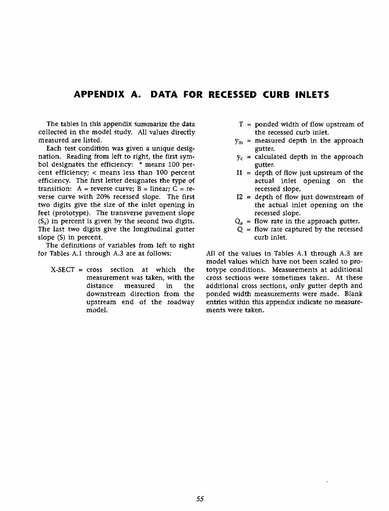
APPENDIX A. DATA FOR RECESSED CURB INLETS

The tables in this appendix summarize the data collected in the model study. All values directly measured are listed.

Each test condition was given a unique desig­nation. Reading from left to right, the first sym­bol designates the efficiency: * means 100 per­cent efficiency; < means less than 100 percent efficiency. The first letter designates the type of transition: A = reverse curve; B = linear; C = re­verse curve with 20% recessed slope. The first two digits give the size of the inlet opening in feet (prototype). The transverse pavement slope (Sx) in percent is given by the second two digits. The last two digits give the longitudinal gutter slope (S) in percent.

The definitions of variables from left to right for Tables A.1 through A.3 are as follows:

X-SECT = cross section at which the measurement was taken, with the distance measured in the downstream direction from the upstream end of the roadway model.

55

T ponded width of flow upstream of the recessed curb inlet.

Ym = measured depth in the approach gutter.

y c = calculated depth in the approach gutter.

I1 = depth of flow just upstream of the actual inlet opening on the recessed slope.

12 = depth of flow just downstream of the actual inlet opening on the recessed slope.

(4 = flow rate in the approach gutter. Q = flow rate captured by the recessed

curb inlet.

All of the values in Tables A.1 through A.3 are model values which have not been scaled to pro­totype conditions. Measurements at additional cross sections were sometimes taken. At these additional cross sections, only gutter depth and ponded width measurements were made. Blank entries within this appendix indicate no measure­ments were taken.

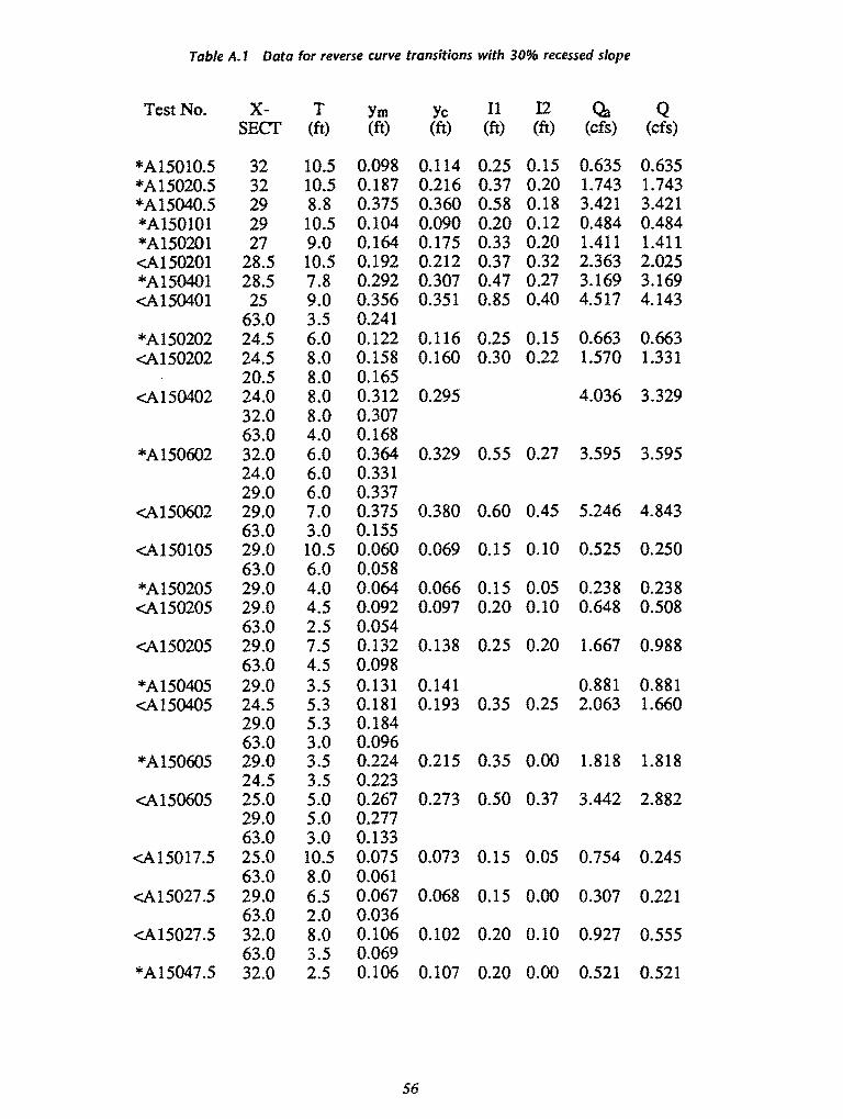
Table A.l Data for reverse curve transitions with 30% recessed slope

Test No. X- T Ym Yc 11 12 Qa Q SECf (ft) (ft) (ft) (ft) (ft) (cfs) (cfs)

*A15010.5 32 10.5 0.098 0.114 0.25 0.15 0.635 0.635 *A15020.5 32 10.5 0.187 0.216 0.37 0.20 1.743 1.743 *A15040.5 29 8.8 0.375 0.360 0.58 0.18 3.421 3.421 *A150101 29 10.5 0.104 0.090 0.20 0.12 0.484 0.484 *A150201 27 9.0 0.164 0.175 0.33 0.20 1.411 1.411 <A150201 28.5 10.5 0.192 0.212 0.37 0.32 2.363 2.025 *A150401 28.5 7.8 0.292 0.307 0.47 0.27 3.169 3.169 <A150401 25 9.0 0.356 0.351 0.85 0.40 4.517 4.143

63.0 3.5 0.241 *A150202 24.5 6.0 0.122 0.116 0.25 0.15 0.663 0.663 <A150202 24.5 8.0 0.158 0.160 0.30 0.22 1.570 1.331

20.5 8.0 0.165 <A150402 24.0 8.0 0.312 0.295 4.036 3.329

32.0 8.0 0.307 63.0 4.0 0.168

*A150602 32.0 6.0 0.364 0.329 0.55 0.27 3.595 3.595 24.0 6.0 0.331 29.0 6.0 0.337

<A150602 29.0 7.0 0.375 0.380 0.60 0.45 5.246 4.843 63.0 3.0 0.155

<A150105 29.0 10.5 0.060 0.069 0.15 0.10 0.525 0.250 63.0 6.0 0.058

*A150205 29.0 4.0 0.064 0.066 0.15 0.05 0.238 0.238 <A150205 29.0 4.5 0.092 0.097 0.20 0.10 0.648 0.508

63.0 2.5 0.054 <A150205 29.0 7.5 0.132 0.138 0.25 0.20 1.667 0.988

63.0 4.5 0.098 *A150405 29.0 3.5 0.131 0.141 0.881 0.881 <A150405 24.5 5.3 0.181 0.193 0.35 0.25 2.063 1.660

29.0 5.3 0.184 63.0 3.0 0.096

*A150605 29.0 3.5 0.224 0.215 0.35 0.00 1.818 1.818 24.5 3.5 0.223

<A150605 25.0 5.0 0.267 0.273 0.50 0.37 3.442 2.882 29.0 5.0 0.277 63.0 3.0 0.133

<A15017.5 25.0 10.5 0.075 0.073 0.15 0.05 0.754 0.245 63.0 8.0 0.061

<A15027.5 29.0 6.5 0.067 0.068 0.15 0.00 0.307 0.221 63.0 2.0 0.036

<A15027.5 32.0 8.0 0.106 0.102 0.20 0.10 0.927 0.555 63.0 3.5 0.069

*A15047.5 32.0 2.5 0.106 0.107 0.20 0.00 0.521 0.521

56

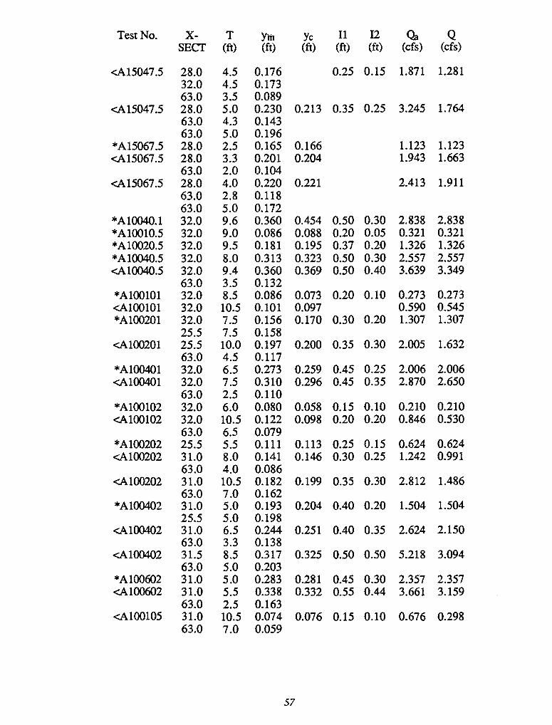
Test No. X- T Yfu Yc 11 12 Qa Q SECf (ft) (ft) (ft) (ft) (ft) (cfs) (cfs)

<A15047.5 28.0 4.5 0.176 0.25 0.15 1.871 1.281 32.0 4.5 0.173 63.0 3.5 0.089

<A15047.5 28.0 5.0 0.230 0.213 0.35 0.25 3.245 1.764 63.0 4.3 0.143 63.0 5.0 0.196

*A15067.5 28.0 2.5 0.165 0.166 1.123 1.123 <A15067.5 28.0 3.3 0.201 0.204 1.943 1.663

63.0 2.0 0.104 <A15067.5 28.0 4.0 0.220 0.221 2.413 1.911

63.0 2.8 0.118 63.0 5.0 0.172

*A10040.1 32.0 9.6 0.360 0.454 0.50 0.30 2.838 2.838 *A10010.5 32.0 9.0 0.086 0.088 0.20 0.05 0.321 0.321 *A10020.5 32.0 9.5 0.181 0.195 0.37 0.20 1.326 1.326 *A10040.5 32.0 8.0 0.313 0.323 0.50 0.30 2.557 2.557 <A10040.5 32.0 9.4 0.360 0.369 0.50 0.40 3.639 3.349

63.0 3.5 0.132 *A100101 32.0 8.5 0.086 0.073 0.20 0.10 0.273 0.273 <A100101 32.0 10.5 0.101 0.097 0.590 0.545 *A100201 32.0 7.5 0.156 0.170 0.30 0.20 1.307 1.307

25.5 7.5 0.158 <A100201 25.5 10.0 0.197 0.200 0.35 0.30 2.005 1.632

63.0 4.5 0.117 *A100401 32.0 6.5 0.273 0.259 0.45 0.25 2.006 2.006 <A100401 32.0 7.5 0.310 0.296 0.45 0.35 2.870 2.650

63.0 2.5 0.110 *A100102 32.0 6.0 0.080 0.058 0.15 0.10 0.210 0.210 <A100102 32.0 10.5 0.122 0.098 0.20 0.20 0.846 0.530

63.0 6.5 0.079 *A100202 25.5 5.5 0.111 0.113 0.25 0.15 0.624 0.624 <A100202 31.0 8.0 0.141 0.146 0.30 0.25 1.242 0.991

63.0 4.0 0.086 <A100202 31.0 10.5 0.182 0.199 0.35 0.30 2.812 1.486

63.0 7.0 0.162 *A100402 31.0 5.0 0.193 0.204 0.40 0.20 1.504 1.504

25.5 5.0 0.198 <A100402 31.0 6.5 0.244 0.251 0.40 0.35 2.624 2.150

63.0 3.3 0.138 <A100402 31.5 8.5 0.317 0.325 0.50 0.50 5.218 3.094

63.0 5.0 0.203 *A100602 31.0 5.0 0.283 0.281 0.45 0.30 2.357 2.357 <A100602 31.0 5.5 0.338 0.332 0.55 0.44 3.661 3.159

63.0 2.5 0.163 <A100105 31.0 10.5 0.074 0.076 0.15 0.10 0.676 0.298

63.0 7.0 0.059

57

Test No. X- T Ym Yc II I2 Oa Q SECf (ft) (ft) (ft) (ft) (ft) (cfs) (cfs)

*A100205 31.0 3.5 0.069 0.074 0.15 0.05 0.316 0.316 <A100205 31.0 6.5 0.129 0.127 0.25 0.20 1.339 0.701

63.0 3.0 0.060 *A100405 28.5 3.5 0.120 0.129 0.25 0.10 0.699 0.699 <A100405 28.0 5.0 0.176 0.188 0.30 0.30 1.902 1.288

63.0 4.0 0.099 <A100405 28.0 6.0 0.262 0.245 0.40 0.35 3.881 1.882

63.0 5.0 0.181 *A100605 28.5 3.0 0.179 0.188 0.30 0.20 1.268 1.268 <A100605 28.5 4.5 0.239 0.251 0.40 0.40 2.749 2.078

63.0 3.3 0.140 <A10017.5 31.0 10.5 0.059 0.055 0.10 0.05 0.346 0.126

63.0 6.0 0.046 <A10027.5 32.0 8.3 0.168 0.152 0.25 0.20 2.647 0.778

63.0 7.0 0.139 *A10047.5 32.0 2.4 0.103 0.098 0.20 0.05 0.412 0.412 <A10047.5 32.0 4.5 0.175 0.179 0.30 0.20 2.047 1.177

63.0 4.0 0.107 <A10047.5 31.5 5.0 0.220 0.201 0.35 0.25 2.799 1.169

63.0 3.5 0.142 <A10047.5 31.5 6.0 0.288 0.252 0.40 0.30 5.118 1.683

63.0 5.0 0.190 *A10067.5 32.0 2.5 0.146 0.151 0.25 0.10 0.873 0.873 <A10067.5 32.0 3.5 0.207 0.206 0.40 0.30 1.990 1.368

63.0 2.5 0.119 <A10067.5 29.0 4.5 0.251 0.256 0.45 0.35 3.536 1.875

63.0 4.5 0.152 *A05020.1 31.5 10.0 0.201 0.223 0.35 0.20 0.856 0.856 *A05040.1 31.5 8.2 0.319 0.393 0.50 0.30 1.932 1.932 *A05020.5 31.5 8.5 0.166 0.162 0.30 0.25 0.810 0.810 <A05020.5 31.5 10.5 0.201 0.193 0.35 0.30 1.295 1.108

63.0 3.2 0.075 *A05040.5 31.5 6.5 0.261 0.262 0.40 0.30 1.462 1.462 <A05040.5 31.5 7.5 0.296 0.292 0.50 0.40 1.958 1.801

63.0 2.5 0.880 <A05040.5 31.5 9.3 0.360 0.357 0.50 0.45 3.343 2.493

63.0 5.0 0.174 *A05060.5 31.5 6.0 0.352 0.348 0.50 0.35 2.079 2.079 <A050101 31.5 10.5 0.126 0.107 0.20 0.20 0.763 0.525

63.0 6.0 0.073 *A050201 31.5 6.5 0.152 0.133 0.25 0.20 0.677 0.677 <A050201 31.5 8.0 0.172 0.151 0.30 0.25 0.951 0.839

63.0 2.5 0.064 <A050201 31.5 9.3 0.200 0.177 0.30 0.30 1.455 1.094

63.0 4.5 0.101 *A050401 31.5 5.0 0.222 0.204 0.35 0.25 1.069 1.069

58

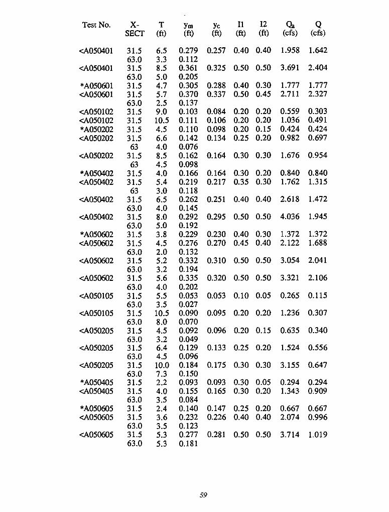
Test No. X- T Ytn Yc 11 12 Oa Q SEer (ft) (ft) (ft) (ft) (ft) (cfs) (cfs)

<.A050401 31.5 6.5 0.279 0.257 0.40 0.40 1.958 1.642 63.0 3.3 0.112

<.A050401 31.5 8.5 0.361 0.325 0.50 0.50 3.691 2.404 63.0 5.0 0.205

*A050601 31.5 4.7 0.305 0.288 0.40 0.30 1.777 1.777 <.A050601 31.5 5.7 0.370 0.337 0.50 0.45 2.711 2.327

63.0 2.5 0.137 <.A050102 31.5 9.0 0.103 0.084 0.20 0.20 0.559 0.303 <.A050102 31.5 10.5 0.111 0.106 0.20 0.20 1.036 0.491 *A050202 31.5 4.5 0.110 0.098 0.20 0.15 0.424 0.424 <.A050202 31.5 6.6 0.142 0.134 0.25 0.20 0.982 0.697

63 4.0 0.076 <.A050202 31.5 8.5 0.162 0.164 0.30 0.30 1.676 0.954

63 4.5 0.098 *A050402 31.5 4.0 0.166 0.164 0.30 0.20 0.840 0.840 <.A050402 31.5 5.4 0.219 0.217 0.35 0.30 1.762 1.315

63 3.0 0.118 <.A050402 31.5 6.5 0.262 0.251 0.40 0.40 2.618 1.472

63.0 4.0 0.145 <.A050402 31.5 8.0 0.292 0.295 0.50 0.50 4.036 1.945

63.0 5.0 0.192 *A050602 31.5 3.8 0.229 0.230 0.40 0.30 1.372 1.372 <.A050602 31.5 4.5 0.276 0.270 0.45 0.40 2.122 1.688

63.0 2.0 0.132 <.A050602 31.5 5.2 0.332 0.310 0.50 0.50 3.054 2.041

63.0 3.2 0.194 <.A050602 31.5 5.6 0.335 0.320 0.50 0.50 3.321 2.106

63.0 4.0 0.202 <.A050105 31.5 5.5 0.053 0.053 0.10 0.05 0.265 0.115

63.0 3.5 0.027 <.A050105 31.5 10.5 0.090 0.095 0.20 0.20 1.236 0.307

63.0 8.0 0.070 <.A050205 31.5 4.5 0.092 0.096 0.20 0.15 0.635 0.340

63.0 3.2 0.049 <.A050205 31.5 6.4 0.129 0.133 0.25 0.20 1.524 0.556

63.0 4.5 0.096 <.A050205 31.5 10.0 0.184 0.175 0.30 0.30 3.155 0.647

63.0 7.3 0.150 *A050405 31.5 2.2 0.093 0.093 0.30 0.05 0.294 0.294 <.A050405 31.5 4.0 0.155 0.165 0.30 0.20 1.343 0.909

63.0 3.5 0.084 *A050605 31.5 2.4 0.140 0.147 0.25 0.20 0.667 0.667 <.A050605 31.5 3.6 0.232 0.226 0.40 0.40 2.074 0.996

63.0 3.5 0.123 <.A050605 31.5 5.3 0.277 0.281 0.50 0.50 3.714 1.019

63.0 5.3 0.181

59

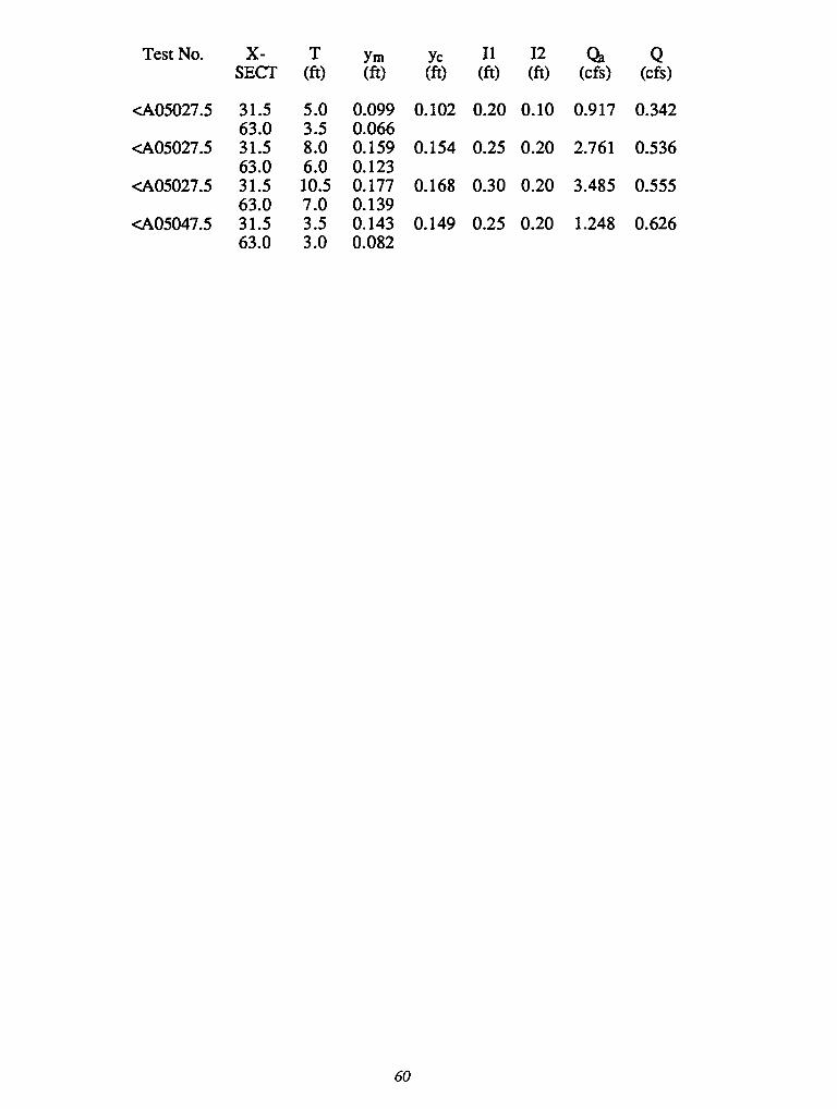
Test No. X- T Ym Yc 11 12 ~ Q SECT (ft) (ft) (ft) (ft) (ft) (cfs) (cfs)

<A05027.5 31.5 5.0 0.099 0.102 0.20 0.10 0.917 0.342 63.0 3.5 0.066

<A05027.5 31.5 8.0 0.159 0.154 0.25 0.20 2.761 0.536 63.0 6.0 0.123

<A05027.5 31.5 10.5 0.177 0.168 0.30 0.20 3.485 0.555 63.0 7.0 0.139

<A05047.5 31.5 3.5 0.143 0.149 0.25 0.20 1.248 0.626 63.0 3.0 0.082

60

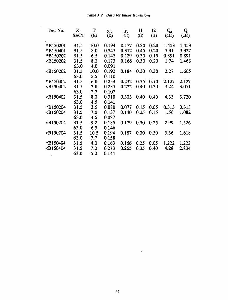
Table A.2 Data for linear transitions

Test No. X- T Ym Yc 11 12 ~ Q SECI' (ft) (ft) (ft) (ft) (ft) (cfs) (cfs)

*B150201 31.5 10.0 0.194 0.177 0.30 0.20 1.453 1.453 *B150401 31.5 8.0 0.347 0.312 0.45 0.20 3.31 3.327 *B150202 31.5 6.5 0.143 0.129 0.30 0.15 0.891 0.891 <B150202 31.5 8.2 0.173 0.166 0.30 0.20 1.74 1.468

63.0 4.0 0.091 <B150202 31.5 10.0 0.192 0.184 0.30 0.30 2.27 1.665

63.0 5.5 0.110 *B150402 31.5 6.0 0.254 0.232 0.35 0.10 2.127 2.127 <B150402 31.5 7.0 0.285 0.272 0.40 0.30 3.24 3.051

63.0 2.7 0.107 <B150402 31.5 8.0 0.310 0.303 0.40 0.40 4.33 3.720

63.0 4.5 0.141 *B150204 31.5 3.5 0.080 0.077 0.15 0.05 0.313 0.313 <B150204 31.5 7.0 0.137 0.140 0.25 0.15 1.56 1.082

63.0 4.5 0.087 <B150204 31.5 9.2 0.185 0.179 0.30 0.25 2.99 1.526

63.0 6.5 0.146 <B150204 31.5 10.5 0.194 0.187 0.30 0.30 3.36 1.618

63.0 7.7 0.158 *B150404 31.5 4.0 0.163 0.166 0.25 0.05 1.222 1.222 <B150404 31.5 7.0 0.273 0.265 0.35 0.40 4.28 2.834

63.0 5.0 0.144

61

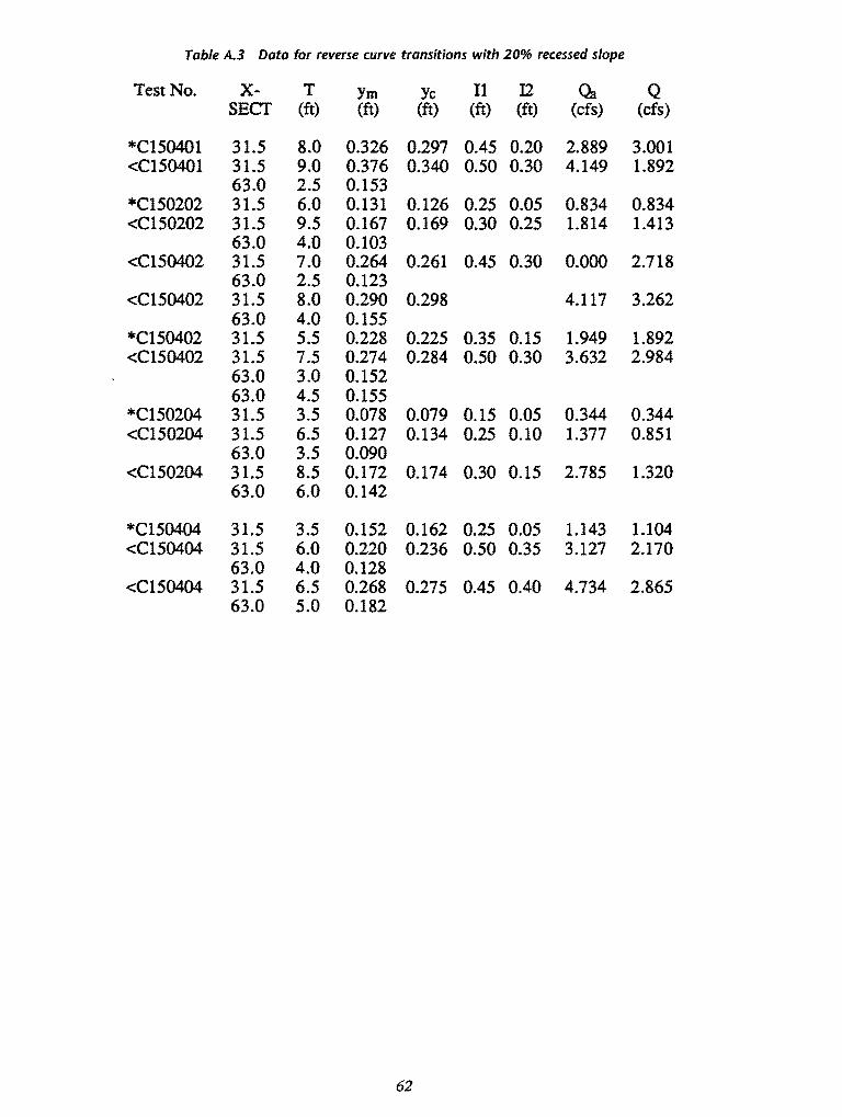
Table A.3 Data far reverse curve transitions with 20% recessed slope

Test No. X- T Ym Yc 11 I2 0.. Q SECT (ft) (ft) (ft) (ft) (ft) (cfs) (cfs)

*C150401 31.5 8.0 0.326 0.297 0.45 0.20 2.889 3.001 <C150401 31.5 9.0 0.376 0.340 0.50 0.30 4.149 1.892

63.0 2.5 0.153 *C150202 31.5 6.0 0.131 0.126 0.25 0.05 0.834 0.834 <C150202 31.5 9.5 0.167 0.169 0.30 0.25 1.814 1.413

63.0 4.0 0.103 <C150402 31.5 7.0 0.264 0.261 0.45 0.30 0.000 2.718

63.0 2.5 0.123 <C150402 31.5 8.0 0.290 0.298 4.117 3.262

63.0 4.0 0.155 *C150402 31.5 5.5 0.228 0.225 0.35 0.15 1.949 1.892 <C150402 31.5 7.5 0.274 0.284 0.50 0.30 3.632 2.984

63.0 3.0 0.152 63.0 4.5 0.155

*C150204 31.5 3.5 0.078 0.079 0.15 0.05 0.344 0.344 <C150204 31.5 6.5 0.127 0.134 0.25 0.10 1.377 0.851

63.0 3.5 0.090 <C150204 31.5 8.5 0.172 0.174 0.30 0.15 2.785 1.320

63.0 6.0 0.142

*C150404 31.5 3.5 0.152 0.162 0.25 0.05 1.143 1.104 <C150404 31.5 6.0 0.220 0.236 0.50 0.35 3.127 2.170

63.0 4.0 0.128 <C150404 31.5 6.5 0.268 0.275 0.45 0.40 4.734 2.865

63.0 5.0 0.182

62

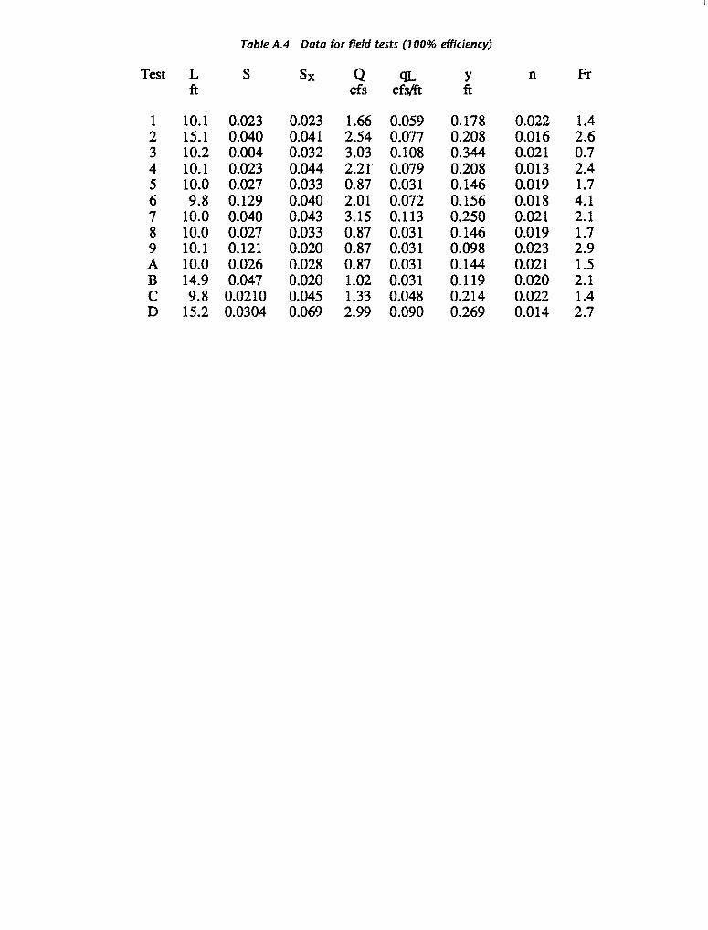
Table A.4 Data for field tests (1 00% efficiency)

Test L s Sx Q QL y n Fr ft cfs cfS/ft ft

1 10.1 0.023 0.023 1.66 0.059 0.178 0.022 1.4 2 15.1 0.040 0.041 2.54 0.077 0.208 0.016 2.6 3 10.2 0.004 0.032 3.03 0.108 0.344 0.021 0.7 4 10.1 0.023 0.044 2.2l 0.079 0.208 0.013 2.4 5 10.0 0.027 0.033 0.87 0.031 0.146 0.019 1.7 6 9.8 0.129 0.040 2.01 0.072 0.156 0.018 4.1 7 10.0 0.040 0.043 3.15 0.113 0.250 0.021 2.1 8 10.0 0.027 0.033 0.87 0.031 0.146 0.019 1.7 9 10.1 0.121 0.020 0.87 0.031 0.098 0.023 2.9 A 10.0 0.026 0.028 0.87 0.031 0.144 0.021 1.5 B 14.9 0.047 0.020 1.02 0.031 0.119 0.020 2.1 c 9.8 0.0210 0.045 1.33 0.048 0.214 0.022 1.4 D 15.2 0.0304 0.069 2.99 0.090 0.269 0.014 2.7

64

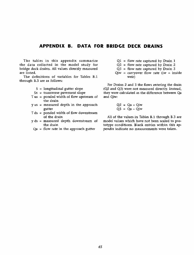
APPENDIX B. DATA FOR BRIDGE DECK DRAINS

The tables in this appendix summarize the data collected in the model study for bridge deck drains. All values directly measured are listed.

The definitions of variables for Tables B.l through B.3 are as follows:

s longitudinal gutter slope Sx = transverse pavement slope

Tus = ponded width of flow upstream of the drain

yus = measured depth in the approach gutter

Tds ponded width of flow downstream of the drain

yds measured depth downstream of the drain

Qa = flow rate in the approach gutter

65

Ql = flow rate captured by Drain 1 Q2 = flow rate captured by Drain 2 Q3 = flow rate captured by Drain 3

Qiw = carryover flow rate (iw = inside weir)

For Drains 2 and 3 the flows entering the drain (Q2 and Q3) were not measured directly. Instead, they were calculated as the difference between Qa and Qiw:

Q2 = Qa- Qiw Q3 = Qa- Qiw

All of the values in Tables B.l through B.3 are model values which have not been scaled to pro­totype conditions. Blank entries within this ap­pendix indicate no measurements were taken.

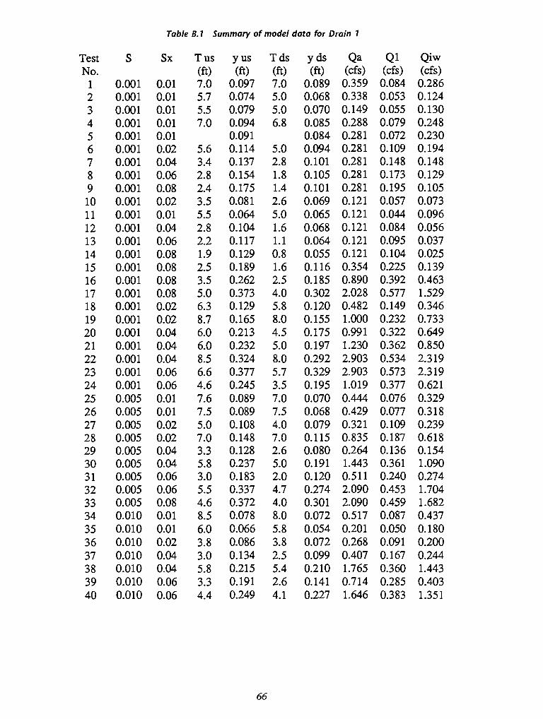
Table B. 7 Summary of model data for Drain 7

Test s Sx Tus yus Tds yds Qa Q1 Qiw No. (ft) (ft) (ft) (ft) (cfs) (cfs) (cfs)

1 0.001 0.01 7.0 0.097 7.0 0.089 0.359 0.084 0.286 2 0.001 0.01 5.7 0.074 5.0 0.068 0.338 0.053 0.124 3 0.001 0.01 5.5 0.079 5.0 0.070 0.149 0.055 0.130 4 0.001 0.01 7.0 0.094 6.8 0.085 0.288 0.079 0.248 5 0.001 0.01 0.091 0.084 0.281 0.072 0.230 6 0.001 0.02 5.6 0.114 5.0 0.094 0.281 0.109 0.194 7 0.001 0.04 3.4 0.137 2.8 0.101 0.281 0.148 0.148 8 0.001 0.06 2.8 0.154 1.8 0.105 0.281 0.173 0.129 9 0.001 0.08 2.4 0.175 1.4 0.101 0.281 0.195 0.105 10 0.001 0.02 3.5 0.081 2.6 0.069 0.121 0.057 0.073 11 0.001 0.01 5.5 0.064 5.0 0.065 0.121 0.044 0.096 12 0.001 0.04 2.8 0.104 1.6 0.068 0.121 0.084 0.056 13 0.001 0.06 2.2 0.117 1.1 0.064 0.121 0.095 0.037 14 0.001 0.08 1.9 0.129 0.8 0.055 0.121 0.104 0.025 15 0.001 0.08 2.5 0.189 1.6 0.116 0.354 0.225 0.139 16 0.001 0.08 3.5 0.262 2.5 0.185 0.890 0.392 0.463 17 0.001 0.08 5.0 0.373 4.0 0.302 2.028 0.577 1.529 18 0.001 0.02 6.3 0.129 5.8 0.120 0.482 0.149 0.346 19 0.001 0.02 8.7 0.165 8.0 0.155 1.000 0.232 0.733 20 0.001 0.04 6.0 0.213 4.5 0.175 0.991 0.322 0.649 21 0.001 0.04 6.0 0.232 5.0 0.197 1.230 0.362 0.850 22 0.001 0.04 8.5 0.324 8.0 0.292 2.903 0.534 2.319 23 0.001 0.06 6.6 0.377 5.7 0.329 2.903 0.573 2.319 24 0.001 0.06 4.6 0.245 3.5 0.195 1.019 0.377 0.621 25 0.005 0.01 7.6 0.089 7.0 0.070 0.444 0.076 0.329 26 0.005 0.01 7.5 0.089 7.5 0.068 0.429 0.077 0.318 27 0.005 0.02 5.0 0.108 4.0 0.079 0.321 0.109 0.239 28 0.005 0.02 7.0 0.148 7.0 0.115 0.835 0.187 0.618 29 0.005 0.04 3.3 0.128 2.6 0.080 0.264 0.136 0.154 30 0.005 0.04 5.8 0.237 5.0 0.191 1.443 0.361 1.090 31 0.005 0.06 3.0 0.183 2.0 0.120 0.511 0.240 0.274 32 0.005 0.06 5.5 0.337 4.7 0.274 2.090 0.453 1.704 33 0.005 0.08 4.6 0.372 4.0 0.301 2.090 0.459 1.682 34 0.010 0.01 8.5 0.078 8.0 0.072 0.517 0.087 0.437 35 0.010 0.01 6.0 0.066 5.8 0.054 0.201 0.050 0.180 36 0.010 0.02 3.8 0.086 3.8 0.072 0.268 0.091 0.200 37 0.010 0.04 3.0 0.134 2.5 0.099 0.407 0.167 0.244 38 0.010 0.04 5.8 0.215 5.4 0.210 1.765 0.360 1.443 39 0.010 0.06 3.3 0.191 2.6 0.141 0.714 0.285 0.403 40 0.010 0.06 4.4 0.249 4.1 0.227 1.646 0.383 1.351

66

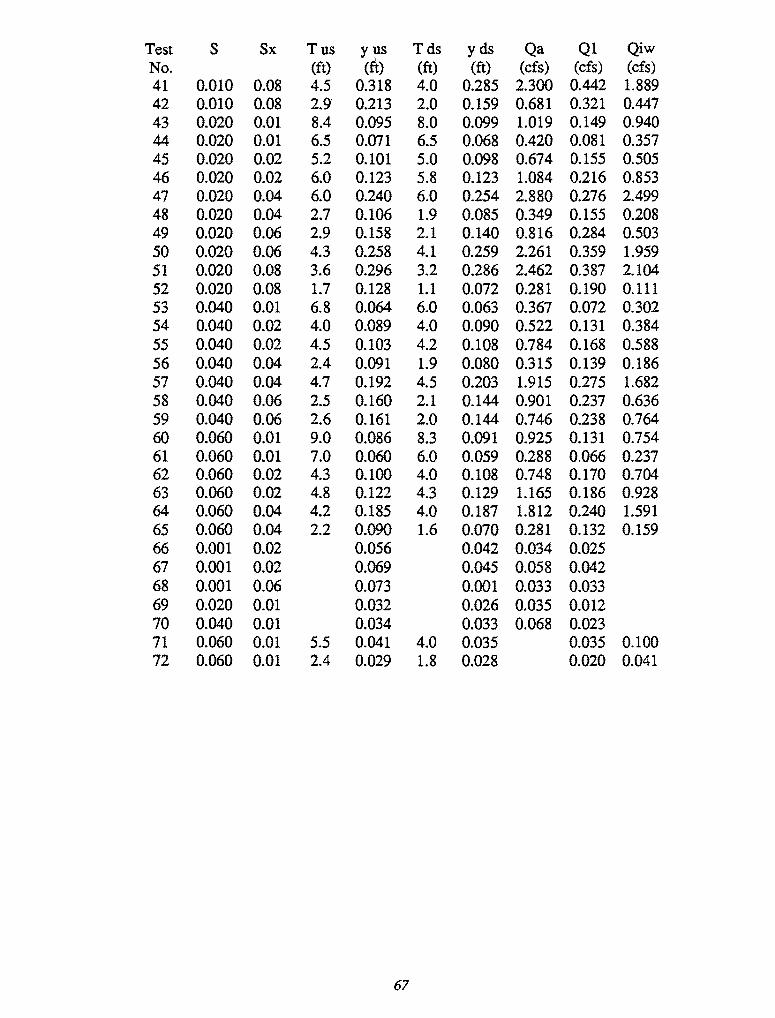
Test s Sx Tus y us Tds yds Qa Ql Qiw No. (ft) (ft) (ft) (ft) (cfs) (cfs) (cfs) 41 0.010 0.08 4.5 0.318 4.0 0.285 2.300 0.442 1.889 42 0.010 0.08 2.9 0.213 2.0 0.159 0.681 0.321 0.447 43 0.020 0.01 8.4 0.095 8.0 0.099 1.019 0.149 0.940 44 0.020 0.01 6.5 0.071 6.5 0.068 0.420 0.081 0.357 45 0.020 0.02 5.2 0.101 5.0 0.098 0.674 0.155 0.505 46 0.020 0.02 6.0 0.123 5.8 0.123 1.084 0.216 0.853 47 0.020 0.04 6.0 0.240 6.0 0.254 2.880 0.276 2.499 48 0.020 0.04 2.7 0.106 1.9 0.085 0.349 0.155 0.208 49 0.020 0.06 2.9 0.158 2.1 0.140 0.816 0.284 0.503 50 0.020 0.06 4.3 0.258 4.1 0.259 2.261 0.359 1.959 51 0.020 0.08 3.6 0.296 3.2 0.286 2.462 0.387 2.104 52 0.020 0.08 1.7 0.128 1.1 0.072 0.281 0.190 0.111 53 0.040 0.01 6.8 0.064 6.0 0.063 0.367 0.072 0.302 54 0.040 0.02 4.0 0.089 4.0 0.090 0.522 0.131 0.384 55 0.040 0.02 4.5 0.103 4.2 0.108 0.784 0.168 0.588 56 0.040 0.04 2.4 0.091 1.9 0.080 0.315 0.139 0.186 57 0.040 0.04 4.7 0.192 4.5 0.203 1.915 0.275 1.682 58 0.040 0.06 2.5 0.160 2.1 0.144 0.901 0.237 0.636 59 0.040 0.06 2.6 0.161 2.0 0.144 0.746 0.238 0.764 60 0.060 0.01 9.0 0.086 8.3 0.091 0.925 0.131 0.754 61 0.060 0.01 7.0 0.060 6.0 0.059 0.288 0.066 0.237 62 0.060 0.02 4.3 0.100 4.0 0.108 0.748 0.170 0.704 63 0.060 0.02 4.8 0.122 4.3 0.129 1.165 0.186 0.928 64 0.060 0.04 4.2 0.185 4.0 0.187 1.812 0.240 1.591 65 0.060 0.04 2.2 0.090 1.6 0.070 0.281 0.132 0.159 66 0.001 0.02 0.056 0.042 0.034 0.025 67 0.001 0.02 0.069 0.045 0.058 0.042 68 0.001 0.06 0.073 0.001 0.033 0.033 69 0.020 0.01 0.032 0.026 0.035 0.012 70 0.040 0.01 0.034 0.033 0.068 0.023 71 0.060 0.01 5.5 0.041 4.0 0.035 0.035 0.100 72 0.060 0.01 2.4 0.029 1.8 0.028 0.020 0.041

67

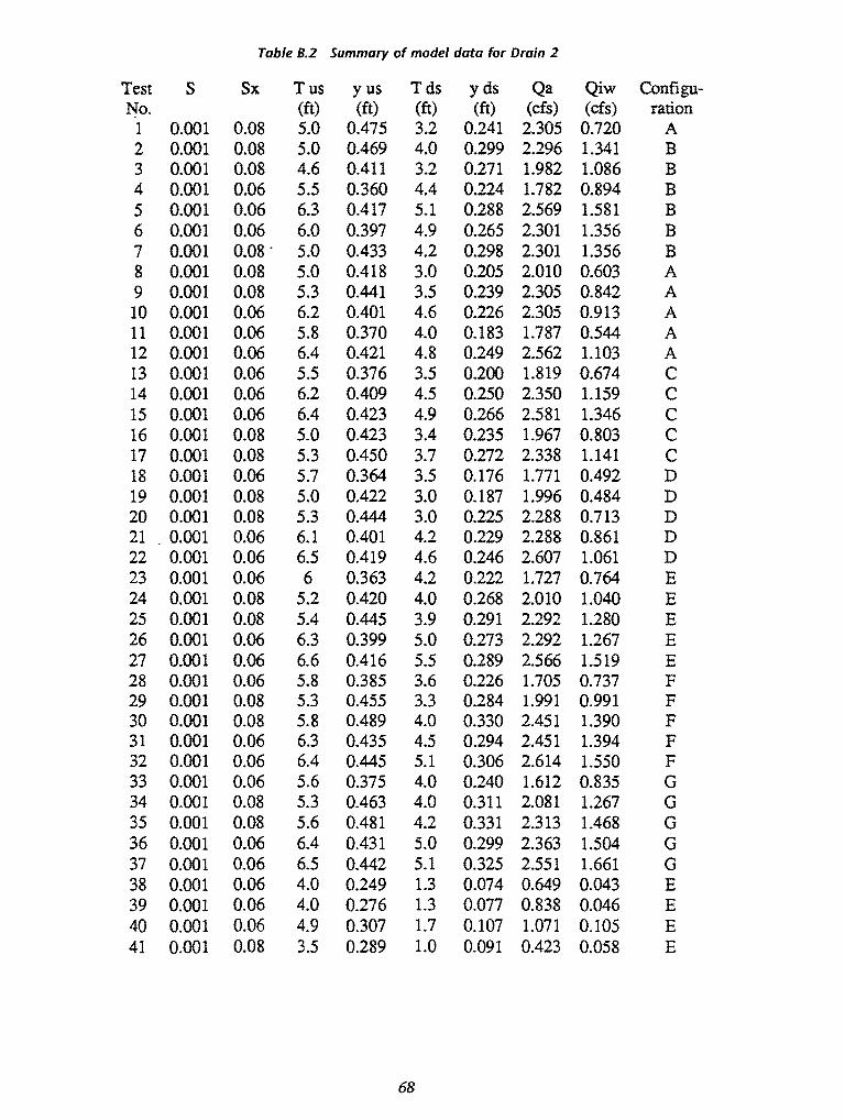
Table 8.2 Summary of model data for Drain 2

Test s Sx Tus yus Tds yds Qa Qiw Configu-No. (ft) (ft) (ft) (ft) (cfs) (cfs) ration

1 0.001 0.08 5.0 0.475 3.2 0.241 2.305 0.720 A 2 0.001 0.08 5.0 0.469 4.0 0.299 2.296 1.341 B 3 0.001 0.08 4.6 0.411 3.2 0.271 1.982 1.086 B 4 0.001 0.06 5.5 0.360 4.4 0.224 1.782 0.894 B 5 0.001 0.06 6.3 0.417 5.1 0.288 2.569 1.581 B 6 0.001 0.06 6.0 0.397 4.9 0.265 2.301 1.356 B 7 0.001 0.08. 5.0 0.433 4.2 0.298 2.301 1.356 B 8 0.001 0.08 5.0 0.418 3.0 0.205 2.010 0.603 A 9 0.001 0.08 5.3 0.441 3.5 0.239 2.305 0.842 A 10 0.001 0.06 6.2 0.401 4.6 0.226 2.305 0.913 A 11 0.001 0.06 5.8 0.370 4.0 0.183 1.787 0.544 A 12 0.001 0.06 6.4 0.421 4.8 0.249 2.562 1.103 A 13 0.001 0.06 5.5 0.376 3.5 0.200 1.819 0.674 c 14 0.001 0.06 6.2 0.409 4.5 0.250 2.350 1.159 c 15 0.001 0.06 6.4 0.423 4.9 0.266 2.581 1.346 c 16 0.001 0.08 5.0 0.423 3.4 0.235 1.967 0.803 c 17 0.001 0.08 5.3 0.450 3.7 0.272 2.338 1.141 c 18 0.001 0.06 5.7 0.364 3.5 0.176 1.771 0.492 D 19 0.001 0.08 5.0 0.422 3.0 0.187 1.996 0.484 D 20 0.001 0.08 5.3 0.444 3.0 0.225 2.288 0.713 D 21 0.001 0.06 6.1 0.401 4.2 0.229 2.288 0.861 D 22 0.001 0.06 6.5 0.419 4.6 0.246 2.607 1.061 D 23 0.001 0.06 6 0.363 4.2 0.222 1.727 0.764 E 24 0.001 0.08 5.2 0.420 4.0 0.268 2.010 1.040 E 25 0.001 0.08 5.4 0.445 3.9 0.291 2.292 1.280 E 26 0.001 0.06 6.3 0.399 5.0 0.273 2.292 1.267 E 27 0.001 0.06 6.6 0.416 5.5 0.289 2.566 1.519 E 28 0.001 0.06 5.8 0.385 3.6 0.226 1.705 0.737 F 29 0.001 0.08 5.3 0.455 3.3 0.284 1.991 0.991 F 30 0.001 0.08 5.8 0.489 4.0 0.330 2.451 1.390 F 31 0.001 0.06 6.3 0.435 4.5 0.294 2.451 1.394 F 32 0.001 0.06 6.4 0.445 5.1 0.306 2.614 1.550 F 33 0.001 0.06 5.6 0.375 4.0 0.240 1.612 0.835 G 34 0.001 0.08 5.3 0.463 4.0 0.311 2.081 1.267 G 35 0.001 0.08 5.6 0.481 4.2 0.331 2.313 1.468 G 36 0.001 0.06 6.4 0.431 5.0 0.299 2.363 1.504 G 37 0.001 0.06 6.5 0.442 5.1 0.325 2.551 1.661 G 38 0.001 0.06 4.0 0.249 1.3 0.074 0.649 0.043 E 39 0.001 0.06 4.0 0.276 1.3 0.077 0.838 0.046 E 40 0.001 0.06 4.9 0.307 1.7 0.107 1.071 0.105 E 41 0.001 0.08 3.5 0.289 1.0 0.091 0.423 0.058 E

68

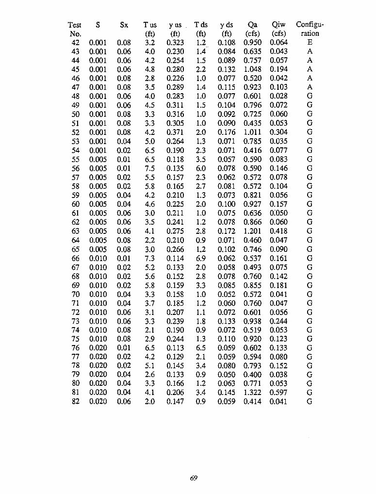
Test s Sx Tus yus Tds yds Qa Qiw Configu-No. (ft) (ft) (ft) (ft) (cfs) (cfs) ration 42 0.001 0.08 3.2 0.323 1.2 0.108 0.950 0.064 E 43 0.001 0.06 4.0 0.230 1.4 0.084 0.635 0.043 A 44 0.001 0.06 4.2 0.254 1.5 0.089 0.757 0.057 A 45 0.001 0.06 4.8 0.280 2.2 0.132 1.048 0.194 A 46 0.001 0.08 2.8 0.226 1.0 0.077 0.520 0.042 A 47 0.001 0.08 3.5 0.289 1.4 0.115 0.923 0.103 A 48 0.001 0.06 4.0 0.283 1.0 0.077 0.601 0.028 G 49 0.001 0.06 4.5 0.311 1.5 0.104 0.796 0.072 G 50 0.001 0.08 3.3 0.316 1.0 0.092 0.725 0.060 G 51 0.001 0.08 3.3 0.305 1.0 0.090 0.435 0.053 G 52 0.001 0.08 4.2 0.371 2.0 0.176 1.011 0.304 G 53 0.001 0.04 5.0 0.264 1.3 0.071 0.785 0.035 G 54 0.001 0.02 6.5 0.190 2.3 0.071 0.416 0.077 G 55 0.005 0.01 6.5 0.118 3.5 0.057 0.590 0.083 G 56 0.005 0.01 7.5 0.135 6.0 0.078 0.590 0.146 G 57 0.005 0.02 5.5 0.157 2.3 0.062 0.572 0.078 G 58 0.005 0.02 5.8 0.165 2.7 0.081 0.572 0.104 G 59 0.005 0.04 4.2 0.210 1.3 0.073 0.821 0.056 G 60 0.005 0.04 4.6 0.225 2.0 0.100 0.927 0.157 G 61 0.005 0.06 3.0 0.211 1.0 0.075 0.636 o:050 G 62 0.005 0.06 3.5 0.241 1.2 0.078 0.866 0.060 G 63 0.005 0.06 4.1 0.275 2.8 0.172 1.201 0.418 G 64 0.005 0.08 2.2 0.210 0.9 0.071 0.460 0.047 G 65 0.005 0.08 3.0 0.266 1.2 0.102 0.746 0.090 G 66 0.010 0.01 7.3 0.114 6.9 0.062 0.537 0.161 G 67 0.010 0.02 5.2 0.133 2.0 0.058 0.493 0.075 G 68 0.010 0.02 5.6 0.152 2.8 0.078 0.760 0.142 G 69 0.010 0.02 5.8 0.159 3.3 0.085 0.855 0.181 G 70 0.010 0.04 3.3 0.158 1.0 0.052 0.572 0.041 G 71 0.010 0.04 3.7 0.185 1.2 0.060 0.760 0.047 G 72 0.010 0.06 3.1 0.207 1.1 0.072 0.601 0.056 G 73 0.010 0.06 3.3 0.239 1.8 0.133 0.938 0.244 G 74 0.010 0.08 2.1 0.190 0.9 0.072 0.519 0.053 G 75 0.010 0.08 2.9 0.244 1.3 0.110 0.920 0.123 G 76 0.020 0.01 6.5 0.113 6.5 0.059 0.602 0.133 G 77 0.020 0.02 4.2 0.129 2.1 0.059 0.594 0.080 G 78 0.020 0.02 5.1 0.145 3.4 0.080 0.793 0.152 G 79 0.020 0.04 2.6 0.133 0.9 0.050 0.400 0.038 G 80 0.020 0.04 3.3 0.166 1.2 0.063 0.771 0.053 G 81 0.020 0.04 4.1 0.206 3.4 0.145 1.322 0.597 G 82 0.020 0.06 2.0 0.147 0.9 0.059 0.414 0.041 G

69

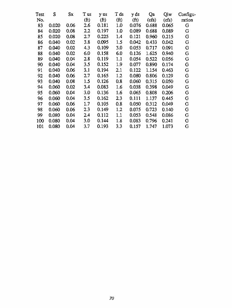
Test s Sx Tus yus Tds yds Qa Qiw Configu-No. (ft) (ft) (ft) (ft) (cfs) (cfs) ration 83 0.020 0.06 2.6 0.181 1.0 0.076 0.688 0.065 G 84 0.020 0.08 2.2 0.197 1.0 0.089 0.688 0.089 G 85 0.020 0.08 2.7 0.225 1.4 0.121 0.960 0.215 G 86 0.040 0.02 3.8 0.095 1.5 0.042 0.433 0.042 G 87 0.040 0.02 4.3 0.109 3.0 0.053 0.717 0.091 G 88 0.040 0.02 6.0 0.158 6.0 0.126 1.625 0.940 G 89 0.040 0.04 2.8 0.119 1.1 0.054 0.522 0.056 G 90 0.040 0.04 3.5 0.152 1.9 0.077 0.890 0.174 G 91 0.040 0.06 3.1 0.194 2.1 0.122 1.154 0.463 G 92 0.040 0.06 2.7 0.165 1.2 0.080 0.806 0.129 G 93 0.040 0.08 1.5 0.126 0.8 0.060 0.315 0.050 G 94 0.060 0.02 3.4 0.083 1.6 0.038 0.398 0.049 G 95 0.060 0.04 3.0 0.136 1.6 0.065 0.808 0.206 G 96 0.060 0.04 3.5 0.162 2.3 0.111 1.137 0.445 G 97 0.060 0.06 1.7 0.105 0.8 0.050 0.312 0.049 G 98 0.060 0.06 2.3 0.149 1.2 0.075 0.723 0.140 G 99 0.080 0.04 2.4 0.112 1.1 0.053 0.548 0.086 G 100 0.080 0.04 3.0 0.144 1.8 0.083 0.796 0.241 G 101 0.080 0.04 3.7 0.193 3.3 0.157 1.747 1.073 G

70

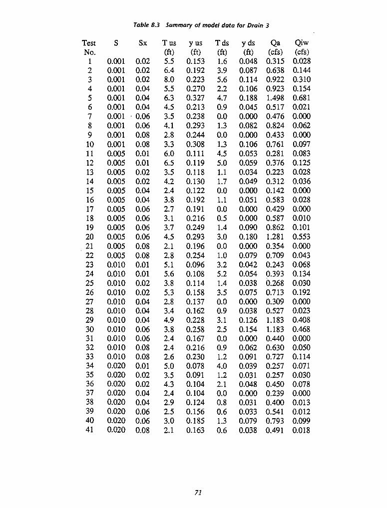
Table 8.3 Summary of model data for Drain 3

Test s Sx Tus y us Tds yds Qa Qiw No. (ft) (ft) (ft) (ft) (cfs) (cfs)

1 0.001 0.02 5.5 0.153 1.6 0.048 0.315 0.028 2 0.001 0.02 6.4 0.192 3.9 0.087 0.638 0.144 3 0.001 0.02 8.0 0.223 5.6 0.114 0.922 0.310 4 0.001 0.04 5.5 0.270 2.2 0.106 0.923 0.154 5 0.001 0.04 6.3 0.327 4.7 0.188 1.498 0.681 6 0.001 0.04 4.5 0.213 0.9 0.045 0.517 0.021 7 0.001 . 0.06 3.5 0.238 0.0 0.000 0.476 0.000 8 0.001 0.06 4.1 0.293 1.3 0.082 0.824 0.062 9 0.001 0.08 2.8 0.244 0.0 0.000 0.433 0.000 10 0.001 0.08 3.3 0.308 1.3 0.106 0.761 0.097 11 0.005 0.01 6.0 0.111 4.5 0.053 0.281 0.083 12 0~005 0.01 6.5 0.119 5.0 0.059 0.376 0.125 13 0.005 0.02 3.5 0.118 1.1 0.034 0.223 0.028 14 0.005 0.02 4.2 0.130 1.7 0.049 0.312 0.036 15 0.005 0.04 2.4 0.122 0.0 0.000 0.142 0.000 16 0.005 0.04 3.8 0.192 1.1 0.051 0.583 0.028 17 0.005 0.06 2.7 0.191 0.0 0.000 0.429 0.000 18 0.005 0.06 3.1 0.216 0.5 0.000 0.587 0.010 19 0.005 0.06 3.7 0.249 1.4 0.090 0.862 0.101 20 0.005 0.06 4.5 0.293 3.0 0.180 1.281 0.553 21 0.005 0.08 2.1 0.196 0.0 0.000 0.354 0.000 22 0.005 0.08 2.8 0.254 1.0 0.079 0.709 0.043 23 0.010 0.01 5.1 0.096 3.2 0.042 0.243 0.068 24 0.010 0.01 5.6 0.108 5.2 0.054 0.393 0.134 25 0.010 0.02 3.8 0.114 1.4 0.038 0.268 0.030 26 0.010 0.02 5.3 0.158 3.5 0.075 0.713 0.192 27 0.010 0.04 2.8 0.137 0.0 0.000 0.309 0.000 28 0.010 0.04 3.4 0.162 0.9 0.038 0.527 0.023 29 0.010 0.04 4.9 0.228 3.1 0.126 1.183 0.408 30 0.010 0.06 3.8 0.258 2.5 0.154 1.183 0.468 31 0.010 0.06 2.4 0.167 0.0 0.000 0.440 0.000 32 0.010 0.08 2.4 0.216 0.9 0.062 0.630 0.050 33 0.010 0.08 2.6 0.230 1.2 0.091 0.727 0.114 34 0.020 0.01 5.0 0.078 4.0 0.039 0.257 0.071 35 0.020 0.02 3.5 0.091 1.2 0.031 0.257 0.030 36 0.020 0.02 4.3 0.104 2.1 0.048 0.450 0.078 37 0.020 0.04 2.4 0.104 0.0 0.000 0.239 0.000 38 0.020 0.04 2.9 0.124 0.8 0.031 0.400 0.013 39 0.020 0.06 2.5 0.156 0.6 0.033 0.541 0.012 40 0.020 0.06 3.0 0.185 1.3 0.079 0.793 0.099 41 0.020 0.08 2.1 0.163 0.6 0.038 0.491 0.018

71

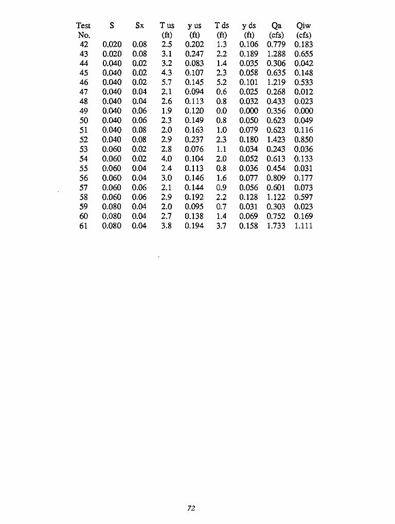
Test s Sx Tus y us Tds y ds Qa Qiw No. (ft) (ft) (ft) (ft) {cfs) (cfs) 42 0.020 0.08 2.5 0.202 1.3 0.106 0.779 0.183 43 0.020 0.08 3.1 0.247 2.2 0.189 1.288 0.655 44 0.040 0.02 3.2 0.083 1.4 0.035 0.306 0.042 45 0.040 0.02 4.3 0.107 2.3 0.058 0.635 0.148 46 0.040 0.02 5.7 0.145 5.2 0.101 1.219 0.533 47 0.040 0.04 2.1 0.094 0.6 0.025 0.268 0.012 48 0.040 0.04 2.6 0.113 0.8 0.032 0.433 0.023 49 0.040 0.06 1.9 0.120 0.0 0.000 0.356 0.000 50 0.040 0.06 2.3 0.149 0.8 0.050 0.623 0.049 51 0.040 0.08 2.0 0.163 1.0 0.079 0.623 0.116 52 0.040 0.08 2.9 0.237 2.3 0.180 1.423 0.850 53 0.060 0.02 2.8 0.076 1.1 0.034 0.243 0.036 54 0.060 0.02 4.0 0.104 2.0 0.052 0.613 0.133 55 0.060 0.04 2.4 0.113 0.8 0.036 0.454 0.031 56 0.060 0.04 3.0 0.146 1.6 0.077 0.809 0.177 57 0.060 0.06 2.1 0.144 0.9 0.056 0.601 0.073 58 0.060 0.06 2.9 0.192 2.2 0.128 1.122 0.597 59 0.080 0.04 2.0 0.095 0.7 0.031 0.303 0.023 60 0.080 0.04 2.7 0.138 1.4 0.069 0.752 0.169 61 0.080 0.04 3.8 0.194 3.7 0.158 1.733 1.111

72

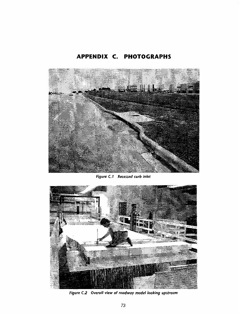
APPENDIX C. PHOTOGRAPHS

Figure C.1 Recessed curb inlet

Figure C.2 Overall view of roadway model looking upstream

73

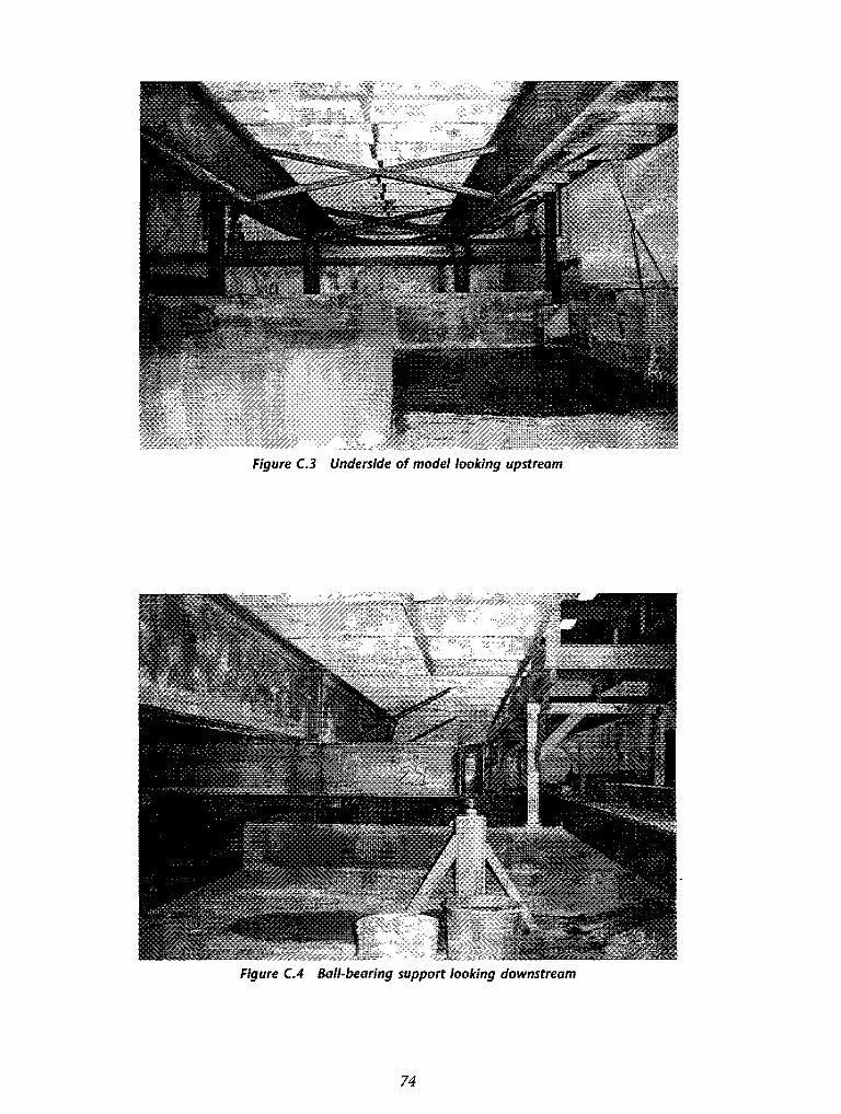
Figure C.3 Underside of mode/looking upstream

Figure C.4 Ball-bearing support looking downstream

74

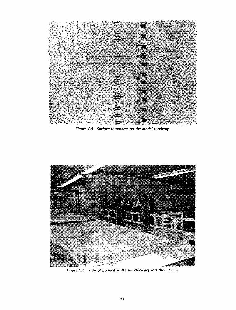
Figure C.5 Surface roughness on the model roadway

Figure C.6 View of ponded width for efficiency less than 100%

75

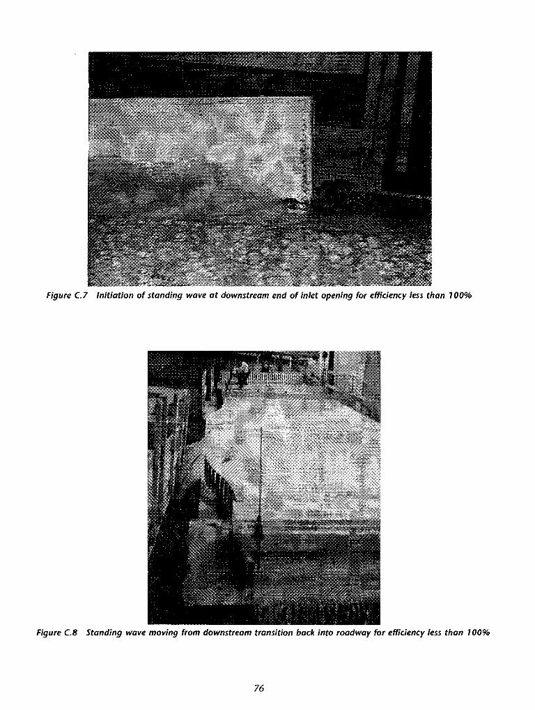
Figure C.l Initiation of standing wave at downstream end of inlet opening for efficiency less than 100%

Figure C.B Standing wave moving from downstream transition back into roadway for efficiency less than 100%

76

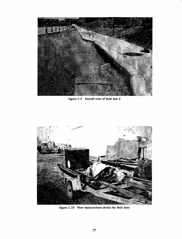
Figure C.9 Overall view of field test 3

Figure C.1 0 Flow measurement device for field tests

77

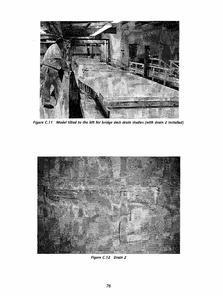
Figure C.11 Model tilted to the left for bridge deck drain studies (with drain 2 installed)

Figure C.12 Drain 2

78

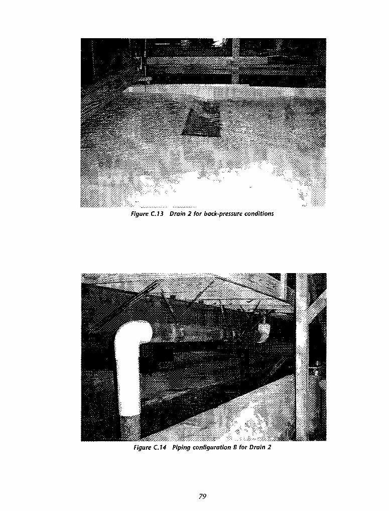
Figure C.13 Drain 2 for back-pressure conditions

Figure C.14 Piping configuration B for Drain 2

79

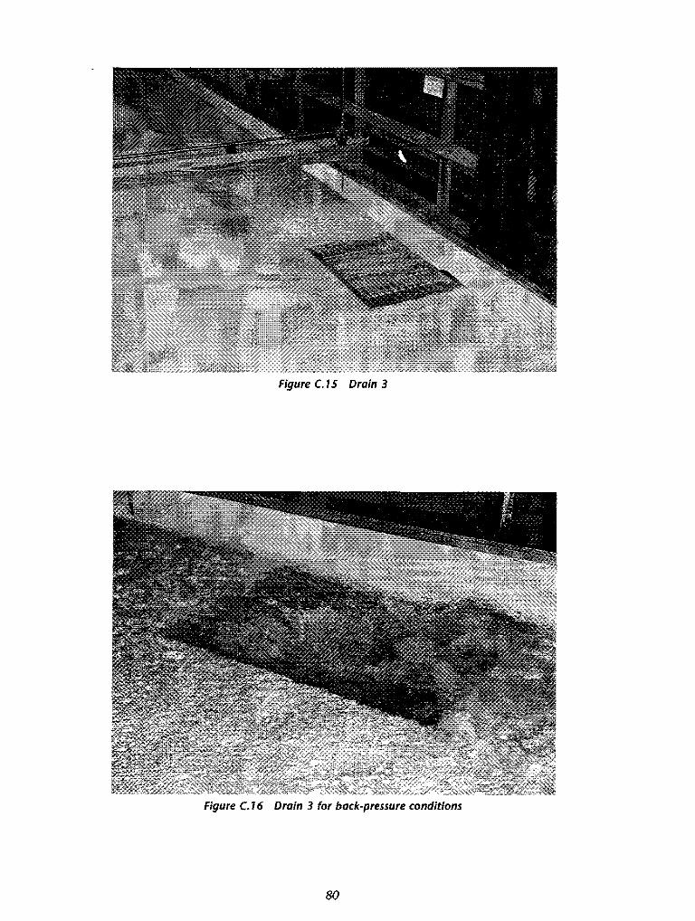
Figure C.15 Drain 3

Figure C.16 Drain 3 for back-pressure conditions

80