TATA September 1996 ECHNICAL STB-33 ULLETIN · TATA September 1996 T ECHNICAL STB-33 B ULLETIN A...
28
STATA September 1996 TECHNICAL STB-33 BULLETIN A publication to promote communication among Stata users Editor Associate Editors H. Joseph Newton Francis X. Diebold, University of Pennsylvania Department of Statistics Joanne M. Garrett, University of North Carolina Texas A & M University Marcello Pagano, Harvard School of Public Health College Station, Texas 77843 James L. Powell, UC Berkeley and Princeton University 409-845-3142 J. Patrick Royston, Royal Postgraduate Medical School 409-845-3144 FAX [email protected] EMAIL Subscriptions are available from StataCorporation, email [email protected], telephone 979-696-4600 or 800-STATAPC, fax 979-696-4601. Current subscription prices are posted at www.stata.com/bookstore/stb.html. Previous Issues are available individually from StataCorp. See www.stata.com/bookstore/stbj.html for details. Submissions to the STB, including submissions to the supporting files (programs, datasets, and help files), are on a nonexclusive, free-use basis. In particular, the author grants to StataCorp the nonexclusive right to copyright and distribute the material in accordance with the Copyright Statement below. The author also grants to StataCorp the right to freely use the ideas, including communication of the ideas to other parties, even if the material is never published in the STB. Submissions should be addressed to the Editor. Submission guidelines can be obtained from either the editor or StataCorp. Copyright Statement. The Stata Technical Bulletin (STB) and the contents of the supporting files (programs, datasets, and help files) are copyright c by StataCorp. The contents of the supporting files (programs, datasets, and help files), may be copied or reproduced by any means whatsoever, in whole or in part, as long as any copy or reproduction includes attribution to both (1) the author and (2) the STB. The insertions appearing in the STB may be copied or reproduced as printed copies, in whole or in part, as long as any copy or reproduction includes attribution to both (1) the author and (2) the STB. Written permission must be obtained from Stata Corporation if you wish to make electronic copies of the insertions. Users of any of the software, ideas, data, or other materials published in the STB or the supporting files understand that such use is made without warranty of any kind, either by the STB, the author, or Stata Corporation. In particular, there is no warranty of fitness of purpose or merchantability, nor for special, incidental, or consequential damages such as loss of profits. The purpose of the STB is to promote free communication among Stata users. The Stata Technical Bulletin (ISSN 1097-8879) is published six times per year by Stata Corporation. Stata is a registered trademark of Stata Corporation. Contents of this issue page an62. Stata 5.0 2 an63. Updates available on the Stata web site 2 sed10.1. Update to pattern 2 sg42.1. Extensions to the regpred command 3 sg49.1. An improved command for paired t tests: Correction 6 sg57. An immediate command for two-way tables 7 sg58. Mountain plots 9 sg59. Index of ordinal variation and Neyman–Barton GOF 10 sg60. Enhancements for the display of estimation results 12 sg61. Bivariate probit models 15 sg62. Hildreth–Houck random coefficients model 21 snp12. Stratified test for trend across ordered groups 24
Transcript of TATA September 1996 ECHNICAL STB-33 ULLETIN · TATA September 1996 T ECHNICAL STB-33 B ULLETIN A...
STATA September 1996
TECHNICAL STB-33
BULLETINA publication to promote communication among Stata users
Editor Associate Editors
H. Joseph Newton Francis X. Diebold, University of PennsylvaniaDepartment of Statistics Joanne M. Garrett, University of North CarolinaTexas A & M University Marcello Pagano, Harvard School of Public HealthCollege Station, Texas 77843 James L. Powell, UC Berkeley and Princeton University409-845-3142 J. Patrick Royston, Royal Postgraduate Medical School409-845-3144 [email protected] EMAIL
Subscriptions are available from Stata Corporation, email [email protected], telephone 979-696-4600 or 800-STATAPC,fax 979-696-4601. Current subscription prices are posted at www.stata.com/bookstore/stb.html.
Previous Issues are available individually from StataCorp. See www.stata.com/bookstore/stbj.html for details.
Submissions to the STB, including submissions to the supporting files (programs, datasets, and help files), are ona nonexclusive, free-use basis. In particular, the author grants to StataCorp the nonexclusive right to copyright anddistribute the material in accordance with the Copyright Statement below. The author also grants to StataCorp the rightto freely use the ideas, including communication of the ideas to other parties, even if the material is never publishedin the STB. Submissions should be addressed to the Editor. Submission guidelines can be obtained from either theeditor or StataCorp.
Copyright Statement. The Stata Technical Bulletin (STB) and the contents of the supporting files (programs,datasets, and help files) are copyright c by StataCorp. The contents of the supporting files (programs, datasets, andhelp files), may be copied or reproduced by any means whatsoever, in whole or in part, as long as any copy orreproduction includes attribution to both (1) the author and (2) the STB.
The insertions appearing in the STB may be copied or reproduced as printed copies, in whole or in part, as longas any copy or reproduction includes attribution to both (1) the author and (2) the STB. Written permission must beobtained from Stata Corporation if you wish to make electronic copies of the insertions.
Users of any of the software, ideas, data, or other materials published in the STB or the supporting files understandthat such use is made without warranty of any kind, either by the STB, the author, or Stata Corporation. In particular,there is no warranty of fitness of purpose or merchantability, nor for special, incidental, or consequential damages suchas loss of profits. The purpose of the STB is to promote free communication among Stata users.
The Stata Technical Bulletin (ISSN 1097-8879) is published six times per year by Stata Corporation. Stata is a registeredtrademark of Stata Corporation.
Contents of this issue page
an62. Stata 5.0 2an63. Updates available on the Stata web site 2
sed10.1. Update to pattern 2sg42.1. Extensions to the regpred command 3sg49.1. An improved command for paired t tests: Correction 6
sg57. An immediate command for two-way tables 7sg58. Mountain plots 9sg59. Index of ordinal variation and Neyman–Barton GOF 10sg60. Enhancements for the display of estimation results 12sg61. Bivariate probit models 15sg62. Hildreth–Houck random coefficients model 21
snp12. Stratified test for trend across ordered groups 24
2 Stata Technical Bulletin STB-33
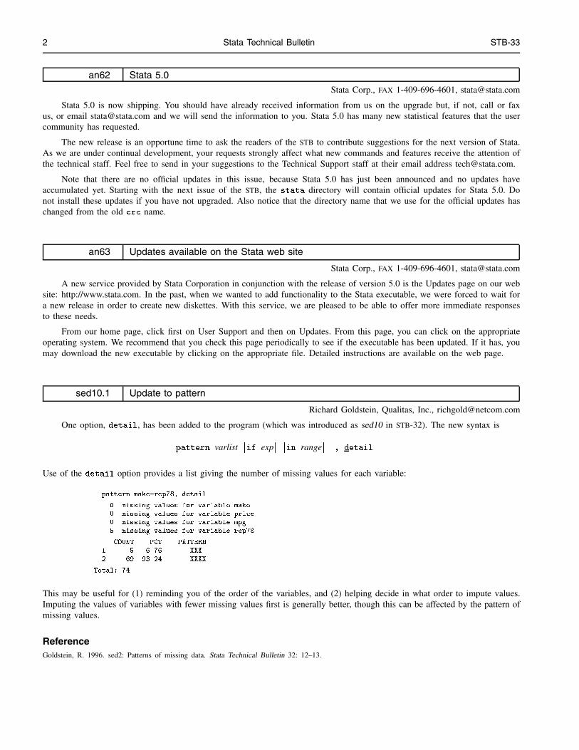
an62 Stata 5.0
Stata Corp., FAX 1-409-696-4601, [email protected]
Stata 5.0 is now shipping. You should have already received information from us on the upgrade but, if not, call or faxus, or email [email protected] and we will send the information to you. Stata 5.0 has many new statistical features that the usercommunity has requested.
The new release is an opportune time to ask the readers of the STB to contribute suggestions for the next version of Stata.As we are under continual development, your requests strongly affect what new commands and features receive the attention ofthe technical staff. Feel free to send in your suggestions to the Technical Support staff at their email address [email protected].
Note that there are no official updates in this issue, because Stata 5.0 has just been announced and no updates haveaccumulated yet. Starting with the next issue of the STB, the stata directory will contain official updates for Stata 5.0. Donot install these updates if you have not upgraded. Also notice that the directory name that we use for the official updates haschanged from the old crc name.
an63 Updates available on the Stata web site
Stata Corp., FAX 1-409-696-4601, [email protected]
A new service provided by Stata Corporation in conjunction with the release of version 5.0 is the Updates page on our website: http://www.stata.com. In the past, when we wanted to add functionality to the Stata executable, we were forced to wait fora new release in order to create new diskettes. With this service, we are pleased to be able to offer more immediate responsesto these needs.
From our home page, click first on User Support and then on Updates. From this page, you can click on the appropriateoperating system. We recommend that you check this page periodically to see if the executable has been updated. If it has, youmay download the new executable by clicking on the appropriate file. Detailed instructions are available on the web page.
sed10.1 Update to pattern
Richard Goldstein, Qualitas, Inc., [email protected]
One option, detail, has been added to the program (which was introduced as sed10 in STB-32). The new syntax is
pattern varlist�if exp
� �in range
� �, detail
�Use of the detail option provides a list giving the number of missing values for each variable:
. pattern make-rep78, detail
0 missing values for variable make
0 missing values for variable price
0 missing values for variable mpg
5 missing values for variable rep78
COUNT PCT PATTERN
1. 5 6.76 XXX.
2. 69 93.24 XXXX
Total: 74
This may be useful for (1) reminding you of the order of the variables, and (2) helping decide in what order to impute values.Imputing the values of variables with fewer missing values first is generally better, though this can be affected by the pattern ofmissing values.
ReferenceGoldstein, R. 1996. sed2: Patterns of missing data. Stata Technical Bulletin 32: 12–13.
Stata Technical Bulletin 3
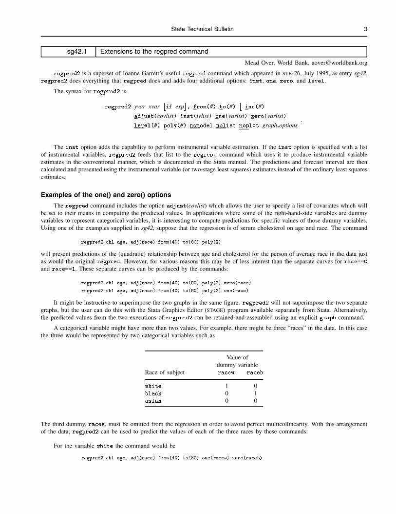
sg42.1 Extensions to the regpred command
Mead Over, World Bank, [email protected]
regpred2 is a superset of Joanne Garrett’s useful regpred command which appeared in STB-26, July 1995, as entry sg42.regpred2 does everything that regpred does and adds four additional options: inst, one, zero, and level.
The syntax for regpred2 is
regpred2 yvar xvar�if exp
�, from(#) to(#)
�inc(#)
adjust(covlist) inst(ivlist) one(varlist) zero(varlist)
level(#) poly(#) nomodel nolist noplot graph options�
The inst option adds the capability to perform instrumental variable estimation. If the inst option is specified with a listof instrumental variables, regpred2 feeds that list to the regress command which uses it to produce instrumental variableestimates in the conventional manner, which is documented in the Stata manual. The predictions and forecast interval are thencalculated and presented using the instrumental variable (or two-stage least squares) estimates instead of the ordinary least squaresestimates.
Examples of the one() and zero() options
The regpred command includes the option adjust(covlist) which allows the user to specify a list of covariates which willbe set to their means in computing the predicted values. In applications where some of the right-hand-side variables are dummyvariables to represent categorical variables, it is interesting to compute predictions for specific values of those dummy variables.Using one of the examples supplied in sg42, suppose that the regression is of serum cholesterol on age and race. The command
. regpred2 chl age, adj(race) from(40) to(80) poly(2)
will present predictions of the (quadratic) relationship between age and cholesterol for the person of average race in the data justas would the original regpred. However, for various reasons this may be of less interest than the separate curves for race==0and race==1. These separate curves can be produced by the commands:
. regpred2 chl age, adj(race) from(40) to(80) poly(2) zero(race)
. regpred2 chl age, adj(race) from(40) to(80) poly(2) one(race)
It might be instructive to superimpose the two graphs in the same figure. regpred2 will not superimpose the two separategraphs, but the user can do this with the Stata Graphics Editor (STAGE) program available separately from Stata. Alternatively,the predicted values from the two executions of regpred2 can be retained and assembled using an explicit graph command.
A categorical variable might have more than two values. For example, there might be three “races” in the data. In this casethe three would be represented by two categorical variables such as
Value ofdummy variable
Race of subject racew raceb
white 1 0black 0 1asian 0 0
The third dummy, racea, must be omitted from the regression in order to avoid perfect multicollinearity. With this arrangementof the data, regpred2 can be used to predict the values of each of the three races by these commands:
For the variable white the command would be
. regpred2 chl age, adj(race) from(40) to(80) one(racew) zero(raceb)

4 Stata Technical Bulletin STB-33
For the variable black:
. regpred2 chl age, adj(race) from(40) to(80) one(raceb) zero(racew)
And for the variable asian:
. regpred2 chl age, adj(race) from(40) to(80) zero(racew raceb)
regpred2 will not permit the user to specify the same variable to be set to both one and zero. The attempt to do so willgenerate an “error 198”.
Examples of the level() and inst() options
Another change introduced in regpred2 is to allow the confidence intervals displayed in the graphs and presented in thepredictions to differ from 95%. regpred2 implements the standard Stata convention of defaulting to a confidence level set bythe S level macro. The S level macro can be overridden by including among the regpred2 options, the option level(#),where # is the desired confidence interval expressed as a percentage.
Here are examples of the application of the level(#) and the inst(ivlist) options. The data used is that in Garrett’s insertin STB-26. First, apply regpred2 as regpred could have been applied, only adding the level(#) option to demonstrate how itworks. Here is the output, including the predicted values and 90% intervals in Figure 1.
. regpred2 chl sbp, f(60) t(300) i(20) adj(age smk) level(90) xlabel ylabel
Source | SS df MS Number of obs = 1218
---------+------------------------------ F( 3, 1214) = 0.37
Model | 1771.65999 3 590.55333 Prob > F = 0.7732
Residual | 1927027.32 1214 1587.33716 R-squared = 0.0009
---------+------------------------------ Adj R-squared = -0.0016
Total | 1928798.98 1217 1584.88001 Root MSE = 39.841
------------------------------------------------------------------------------
chl | Coef. Std. Err. t P>|t| [90% Conf. Interval]
---------+--------------------------------------------------------------------
sbp | .0404827 .0438582 0.923 0.356 -.0317128 .1126782
age | -.0632856 .131533 -0.481 0.631 -.2798034 .1532323
smk | -1.328942 2.399776 -0.554 0.580 -5.279237 2.621353
_cons | 210.093 8.212943 25.581 0.000 196.5736 223.6124
------------------------------------------------------------------------------
Predicted Values and 90% Confidence Intervals
Outcome Variable: Serum cholesterol -- chl
Independent Variable: Systolic blood pressure -- sbp
Covariates: age smk
Instruments:
Variables set to Zero:
Variables set to One:
Total Observations: 1218
Confidence interval: 90
sbp pred_y lower upper
1. 60 208.2786 201.8328 214.7245
2. 80 209.0883 204.0052 214.1713
3. 100 209.8979 206.1179 213.678
4. 120 210.7076 208.0801 213.3351
5. 140 211.5172 209.5984 213.4361
6. 160 212.3269 210.1766 214.4772
7. 180 213.1365 210.0174 216.2556
8. 200 213.9462 209.5876 218.3048
9. 220 214.7558 209.0612 220.4505
10. 240 215.5655 208.4927 222.6383
11. 260 216.3752 207.9027 224.8476
12. 280 217.1848 207.3002 227.0694
13. 300 217.9945 206.69 229.2989
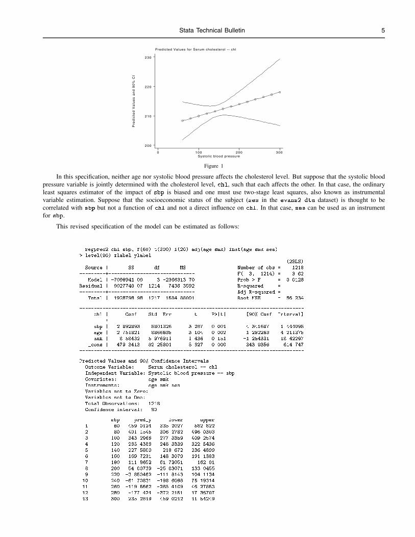
Stata Technical Bulletin 5
Predicted Values for Serum cholesterol -- chl
Pre
dic
ted
Va
lue
s a
nd
90
% C
I
Systol ic blood pressure0 100 200 300
200
210
220
230
Figure 1
In this specification, neither age nor systolic blood pressure affects the cholesterol level. But suppose that the systolic bloodpressure variable is jointly determined with the cholesterol level, chl, such that each affects the other. In that case, the ordinaryleast squares estimator of the impact of sbp is biased and one must use two-stage least squares, also known as instrumentalvariable estimation. Suppose that the socioeconomic status of the subject (ses in the evans2.dta dataset) is thought to becorrelated with sbp but not a function of chl and not a direct influence on chl. In that case, ses can be used as an instrumentfor sbp.
This revised specification of the model can be estimated as follows:
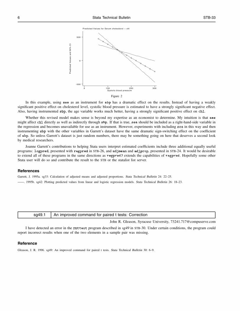
. regpred2 chl sbp, f(60) t(300) i(20) adj(age smk) inst(age smk ses)
> level(90) xlabel ylabel
(2SLS)
Source | SS df MS Number of obs = 1218
---------+------------------------------ F( 3, 1214) = 3.62
Model | -7098941.09 3 -2366313.70 Prob > F = 0.0128
Residual | 9027740.07 1214 7436.3592 R-squared = .
---------+------------------------------ Adj R-squared = .
Total | 1928798.98 1217 1584.88001 Root MSE = 86.234
------------------------------------------------------------------------------
chl | Coef. Std. Err. t P>|t| [90% Conf. Interval]
---------+--------------------------------------------------------------------
sbp | -2.892893 .8801326 -3.287 0.001 -4.341687 -1.444098
age | 2.751821 .8866685 3.104 0.002 1.292268 4.211375
smk | 8.58432 5.976911 1.436 0.151 -1.254331 18.42297
_cons | 479.3413 82.25801 5.827 0.000 343.9356 614.747
------------------------------------------------------------------------------
Predicted Values and 90% Confidence Intervals
Outcome Variable: Serum cholesterol -- chl
Independent Variable: Systolic blood pressure -- sbp
Covariates: age smk
Instruments: age smk ses
Variables set to Zero:
Variables set to One:
Total Observations: 1218
Confidence interval: 90
sbp pred_y lower upper
1. 60 459.0124 335.2027 582.822
2. 80 401.1545 306.2782 496.0308
3. 100 343.2966 277.3359 409.2574
4. 120 285.4388 248.3339 322.5436
5. 140 227.5809 218.672 236.4899
6. 160 169.7231 148.3079 191.1383
7. 180 111.8652 61.72051 162.01
8. 200 54.00739 -25.03071 133.0455
9. 220 -3.850462 -111.8143 104.1134
10. 240 -61.70831 -198.6098 75.19314
11. 260 -119.5662 -285.4109 46.27853
12. 280 -177.424 -372.2151 17.36707
13. 300 -235.2819 -459.0212 -11.54249
6 Stata Technical Bulletin STB-33
Predicted Values for Serum cholesterol -- chl
Pre
dic
ted
Va
lue
s a
nd
90
% C
I
Systol ic blood pressure0 100 200 300
-500
0
500
Figure 2
In this example, using ses as an instrument for sbp has a dramatic effect on the results. Instead of having a weaklysignificant positive effect on cholesterol level, systolic blood pressure is estimated to have a strongly significant negative effect.Also, having instrumented sbp, the age variable works much better, having a strongly significant positive effect on chl.
Whether this revised model makes sense is beyond my expertise as an economist to determine. My intuition is that sesmight affect chl directly as well as indirectly through sbp. If that is true, ses should be included as a right-hand-side variable inthe regression and becomes unavailable for use as an instrument. However, experiments with including ses in this way and theninstrumenting sbp with the other variables in Garrett’s dataset have the same dramatic sign-switching effect on the coefficientof sbp. So unless Garrett’s dataset is just random numbers, there may be something going on here that deserves a second lookby medical researchers.
Joanne Garrett’s contributions to helping Stata users interpret estimated coefficients include three additional equally usefulprograms: logpred, presented with regpred in STB-26, and adjmean and adjprop, presented in STB-24. It would be desirableto extend all of these programs in the same directions as regpred2 extends the capabilities of regpred. Hopefully some otherStata user will do so and contribute the result to the STB or the statalist list server.
ReferencesGarrett, J. 1995a. sg33: Calculation of adjusted means and adjusted proportions. Stata Technical Bulletin 24: 22–25.
——. 1995b. sg42: Plotting predicted values from linear and logistic regression models. Stata Technical Bulletin 26: 18–23.
sg49.1 An improved command for paired t tests: Correction
John R. Gleason, Syracuse University, [email protected]
I have detected an error in the rmttest program described in sg49 in STB-30. Under certain conditions, the program couldreport incorrect results when one of the two elements in a sample pair was missing.
Reference
Gleason, J. R. 1996. sg49: An improved command for paired t tests. Stata Technical Bulletin 30: 6–9.
Stata Technical Bulletin 7
sg57 An immediate command for two-way tables
Nicholas J. Cox, University of Durham, UK, FAX (011)-44-91-374-2456, [email protected]
The syntax for the tab2i command is
tab2i #11 #12�: : :
�n #21 #22
�: : :
� �n : : :
� �, replace
�where #11, #12, etc., are zeros or positive integers showing the frequencies in a two-way table, and backslashes separate rowsof the table. There must be at least two rows and at least two columns in the table.
Option
replace indicates that the variables listed by the command are to be left as the current data in place of whatever data werethere. These variables are row and column indices, observed and expected frequencies, and Pearson and adjusted residuals.
Explanation
A chi-squared test for association of the row and column variables in a two-way table of frequencies is featured in most firstcourses in statistics. In Stata, this test is provided by the immediate command tabi or by the command tabulate. However,neither produces output of expected (fitted, predicted) frequencies or of residuals. Most data analysts wish to glance at leastbriefly at such results.
tab2i is an alternative to tabi that does produce this output. In a two-way table of frequencies, the observed frequency inrow i and column j of the table yij is compared with the expected frequency byij . Under the null hypothesis of independence,the expected frequencies are calculated from row totals yi+, column totals y+j , and the table total y++ by
byij = yi+ y+j
y++
The chi-squared statistic is then
�2 =
X (yij � byij)2byijThe residuals produced by tab2i come in two flavors. First, Pearson residuals (also called standardized or chi-residuals)
are the (appropriately signed) square roots of each cell’s contribution to the Pearson chi-squared statistic. The Pearson residualsare thus
yij � byijpbyijUnder the null hypothesis, the Pearson residuals approximately follow Gaussian (normal) distributions with mean 0 and varianceless than 1. Consequently, one rough rule of thumb is to look especially carefully at any residual greater than 2 in magnitude.
Second, adjusted residuals are Pearson residuals divided by an estimate of their standard errors�1�
yi+
y++
��1�
y+j
y++
�so that they are distributed more like Gaussians with mean 0 and variance 1.
Example
Jacqueline Tivers (1985) interviewed 400 women with young children in the London Borough of Merton in September1977. In one analysis, she looked at the cross-tabulation of the age at which women finished full-time education and whetherthey used a library regularly. The table of frequencies did not come with a chi-squared statistic or residuals.
8 Stata Technical Bulletin STB-33
Regular use of libraryAge left full-time education No Yes Total
Below 16 years 124 21 14516 years 73 30 10317-18 years 55 29 8419 years or older 27 41 68
Total 279 121 400
Source of data: Tivers (1985, 173)
We type in the data just as for tabi, with backslashes separating the rows of the table:
. tab2i 124 21 n 73 30 n 55 29 n 27 41
residuals
row col observed expected Pearson adjusted
1 1 124 101.138 2.273 5.177
1 2 21 43.862 -3.452 -5.177
2 1 73 71.843 0.137 0.288
2 2 30 31.157 -0.207 -0.288
3 1 55 58.590 -0.469 -0.959
3 2 29 25.410 0.712 0.959
4 1 27 47.430 -2.966 -5.920
4 2 41 20.570 4.505 5.920
Pearson chi2(3) = 46.9646 Pr = 0.000
The chi-squared statistic is overwhelmingly significant and the pattern of residuals, especially the adjusted residuals, clearlyshows a monotonic relationship. In fact, Tivers gave a result for Goodman–Kruskal gamma, which might be thought moreappropriate by some analysts than chi-squared for a relationship between variables on ordinal scales. (See the entry for tabulatein the Stata Reference Manuals for an explanation of gamma.)
tab2i has one option: replace indicates that the variables listed by the command are to be left as the current data inplace of whatever data were there. These variables are row and column indices, observed and expected frequencies, and Pearsonand adjusted residuals.
Discussion
There are several other possible definitions of residuals in the literature. For more information on this or other points, seea standard text on categorical data analysis. For example, Gilbert (1993) and Agresti (1996) assume a modest background instatistics, whereas Bishop, Fienberg, and Holland (1975) and Agresti (1990) are more advanced. Haberman (1973) is a key paperintroducing adjusted residuals.
For more advanced work with two-way tables, use Judson’s loglinear analysis command loglin from STB-6 and STB-8(Judson, 1992a, 1992b) or the even more general glm command. These allow many models other than that of independence tobe fitted and tested. On the other hand, students and others who may not be familiar with these methods might find tab2i moreaccessible for its own elementary task.
In short, tab2i is a minimal first look at a two-way table. Most of the code was gleefully cribbed from tabi. Such theftfollowed the observation that if there are no data in memory when tabi is invoked, then the data supplied in the table are leftbehind as three variables, row, col, and pop.
Acknowledgment
William Gould of Stata Corporation provided many useful suggestions for improvement of tab2i, but he is not responsiblefor any of its deficiencies.
ReferencesAgresti, A. 1990. Categorical Data Analysis. New York: John Wiley.
——. 1996. An Introduction to Categorical Data Analysis. New York: John Wiley.
Stata Technical Bulletin 9
Bishop, Y. M. M., S. E. Fienberg, and P. W. Holland. 1975. Discrete Multivariate Analysis. Cambridge, MA: MIT Press.
Gilbert, N. 1993. Analyzing tabular data: loglinear and logistic models for social researchers. London: UCL Press.
Haberman, S. J. 1973. The analysis of residuals in cross-classified tables. Biometrics 29: 205–220.
Judson, D. H. 1992a. smv5: Performing loglinear analysis of cross-classifications. Stata Technical Bulletin 6: 7–17.
——. 1992b. smv5.1: Loglinear analysis of cross-classifications, update. Stata Technical Bulletin 8: 18.
Tivers, J. 1985. Women Attached: The Daily Lives of Women with Young Children. Beckenham, UK: Croom Helm.
sg58 Mountain plots
Richard Goldstein, Qualitas, Inc., [email protected]
There are numerous options, both in Stata and in the literature, for graphically displaying univariate distributions. Examplesin Stata include box plots, probability plots, histograms, stem-and-leaf plots, etc. One family of such plots display the empiricaldistribution function (EDF). The mountain plot presented here is a member of this family.
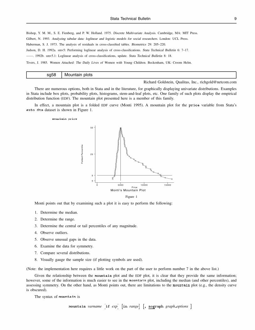
In effect, a mountain plot is a folded EDF curve (Monti 1995). A mountain plot for the price variable from Stata’sauto.dta dataset is shown in Figure 1.
. mountain price
Fo
lde
d P
erc
en
tile
Mont i 's Mountain PlotPrice
0 5000 10000 15000
0
5
25
50
Figure 1
Monti points out that by examining such a plot it is easy to perform the following:
1. Determine the median.
2. Determine the range.
3. Determine the central or tail percentiles of any magnitude.
4. Observe outliers.
5. Observe unusual gaps in the data.
6. Examine the data for symmetry.
7. Compare several distributions.
8. Visually gauge the sample size (if plotting symbols are used).
(Note: the implementation here requires a little work on the part of the user to perform number 7 in the above list.)
Given the relationship between the mountain plot and the EDF plot, it is clear that they provide the same information;however, some of the information is much easier to see in the mountain plot, including the median (and other percentiles), andassessing symmetry. On the other hand, as Monti points out, there are limitations to the mountain plot (e.g., the density curveis obscured).
The syntax of mountain is
mountain varname�if exp
� �in range
� �, nograph graph options
�
10 Stata Technical Bulletin STB-33
Unless the nograph option is used, a plot will automatically be displayed. By default, the graph options used includeylabel, xlabel, yline(5) (so one can see the 5th and 95th percentiles), xline(median), and c(l).
As implemented, the command can only be used for one variable at a time. However, a new variable foldx is left in thedataset (which is quietly dropped on reuse of the command). If the user has more than one measure of something and wants tocompare the plots, then rename foldx to something meaningful and rerun; then one can plot the two mountains against whateach is measuring (be sure to sort on the x variable before graphing).
Note that a variant of egen rank is used with this command (and supplied on the disk as grank2.ado) that does notgive the average rank to tied values since this would give a misleading plot in many cases. Instead unique ranks are given toall values even if tied. Tied values can be seen in the plot because they are joined by absolutely vertical lines as long as theydo not cross the median; if they cross the median, then they are joined by absolutely horizontal lines.
Reference
Monti, K. L. 1995. Folded empirical distribution function curves—mountain plots. The American Statistician 49: 342–345.
sg59 Index of ordinal variation and Neyman–Barton GOF
Richard Goldstein, Qualitas, Inc., [email protected]
What do you do when you have a variable with ordered categories? While there are numerous answers to this question whenone has covariates, or other variables, there are few good answers in the univariate situation. This insert presents a measure,called the index of variation (iov), and test of statistical significance, of the amount of variation in an ordered variable. Theclosely related index of ordinal consensus is also presented. An associated program, nbgof, used in testing the significance ofthe iov is also presented.
The syntax of iov isiov varname
�if exp
� �in range
� �, rows(#) actual
�The program provides a measure of variability (and its complement) for ordinal variables. The complement measures lack ofvariability. Each variable can either have the same, fixed, number of categories, set by the user, or, by using the option actual,you can use the actually existing number of categories. If you don’t use either option, the default number is 5. These optionsallow for the situation when the variable as defined has x categories, but the particular sample at issue does not use all thecategories.
The iov is 0 (and ioc is 1) when all values fall into one category; the iov is 1 (and the ioc is 0) when extreme polarizationis present. The p-value for a goodness-of-fit test (where the uniform distribution is the null hypothesis; see nbgof) is alsopresented. The Berry–Mielke (1994) article gives an algorithm for an exact test, and they also make FORTRAN code for this testavailable. The test that I have implemented here is not exact.
Note that the program expects data in the form of individual observations; if data are frequency weighted, they should beexpanded prior to using this program.
Two options are allowed: rows(#) and actual. If you use neither, the program assumes that every variable called shouldbe treated as though it has five categories. If you use both options, only the actual option will be used.
The default value for rows is 5, chosen simply because the most usual use for this in my own work is with 5-point Likertscales. Note that if your variable has other than 5 possible values you should definitely use this option as these calculations willbe wrong if you have the wrong number of categories.
The use of actual tells the program to use the actually existing number of categories. Each user must decide whether touse the possible number of categories or the actual number in every case, but in my experience it is the possible number thatusually, but not always, of interest. Note further that using this program with the possible number of rows given eases use onnew datasets that are based on the same data collection form.
If you use the actual option, then the output tells you how many rows there are for each variable; if you use no option,or use the rows option, then this information is not supplied.
Note that the originators of this prefer a randomization test; the test here (see below) is offered as an approximation.
Stata Technical Bulletin 11
Examples
The first example is from the originators of this statistic (Berry and Mielke 1994):
. iov likert
Variable IOV IOC p-value
---------+------------------------------------
likert | 0.6976 0.3024 0.0440
Next we use the same data, except that we have duplicated the above variable and then set all cases with a value of 5 to missing:
. replace lik2 = . if lik2==5
(4 real changes made, 4 to missing)
. iov lik*, actual
Variable IOV IOC p-value rows
---------+------------------------------------------------
likert | 0.6976 0.3024 0.0440 5
lik2 | 0.8116 0.1884 0.0000 4
Next is a made-up example. There are two variables and 40 observations in the dataset. Variable x consists of just thenumbers 1–40, while variable y has 10 each of the values 1, 2, 3, and 4. I start with a brief description of the two variables:
. su x y
Variable | Obs Mean Std. Dev. Min Max
---------+-----------------------------------------------------
x | 40 20.5 11.69045 1 40
y | 40 2.5 1.132277 1 4
. iov x, rows(40)
Variable IOV IOC p-value
---------+------------------------------------
x | 0.6833 0.3167 0.9364
. iov y, rows(4)
Variable IOV IOC p-value
---------+------------------------------------
y | 0.8333 0.1667 0.0000
Note the odd result for these two variables when the rows option is not used; the p-value is not affected, but the values of thestatistics are
. iov x y
Variable IOV IOC p-value
---------+------------------------------------
x | 0.0250 0.9750 0.9364
y | 0.6250 0.3750 0.0000
The Neyman–Barton smooth goodness-of-fit test
The syntax of nbgof isnbgof varname
�if exp
� �in range
�This program performs a Neyman–Barton smooth goodness-of-fit test of order 2. The test result is asymptotically distributed aschi-squared with 2 df. This is used for testing of uniformity (i.e., a uniform distribution). The test is valid for U(0; 1), so if thedata are outside this range they are transformed to inside the range using a standard transformation (Stephens 1986).
The output consists of four pieces of information for each variable: (1) the value of the test statistic; (2) its p-value; (3) thevalue of �
U , one of the two components of the test statistic and also a test statistic; (4) the value of S2, the other componentof the test statistic, and also a test statistic. p-values are not given for �
U and S2 as I have been unable to find a reasonable
approximation to the tables given in Stephens. (Each of these is asymptotically standard normal.) The Neyman–Barton test isequal to the sum of the squared values of the component tests.
The data are expected to be in unweighted form. If they are frequency weighted, use Stata’s expand command.
No options are allowed.

12 Stata Technical Bulletin STB-33
Example
The following uses the example given in Stephens (1986):
. input u
u
1. .004
2. .304
3. .612
4. .748
5. .771
6. .806
7. .850
8. .885
9. .906
10. .977
11. end
. nbgof u
Neyman-Barton
Variable Smooth GOF Test p-value U-bar S-squared
---------+------------------------------------------------------
u | 6.437 0.0400 2.041 1.507
ReferencesBerry, K. J. and P. W. Mielke, Jr. 1994. A test of significance for the index of ordinal variation. Perceptual and Motor Skills 79: 1291–1295.
Stephens, M. A. 1986. Tests for the uniform distribution. In Goodness-of-Fit Techniques, eds. R. B. D’Agostino and M. A. Stephens. New York:Marcel Dekker.
sg60 Enhancements for the display of estimation results
Jeroen Weesie, Utrecht University, Netherlands, [email protected]
The regular Stata output of estimation commands comprises parameter estimates, standard errors, z or t statistics, p-values,and confidence intervals. Clearly, there is a lot of redundancy in this information. For instance, z and t statistics are simply theratios of the estimates and their standard errors. (Note that this is not fully correct: In exponentiated form, z and t statistics arenot transformed by Stata.) Hypotheses testing is possible either via confidence intervals or via p-values.
In practice, many researchers only consider a few of these numbers, in particular the parameter estimates and the associatedp-values. Thus, precious “display space” seems to be wasted. Indeed, at the same time, Stata’s regular output does not containpieces of information that I find quite useful.
First, Stata’s variable names, as are all of its identifiers, are restricted to length 8. In many cases, this is hardly sufficient toproduce meaningful names. For instance, in many surveys, variables are named V013aj, etc. Additionally, the names of variablesproduced and named automatically by programs such as xi are hardly more understandable than assembler mnemonics. Variablelabels, even those produced automatically by xi, are usually easy to understand. These labels could simply be included in theoutput.
Second, to interpret the “size of effects” it is useful to see the location and scale of variables along with the parameterestimates. This practice is followed by many statistical programs including SPSS, BMDP, and LIMDEP.
This insert describes a program diest, that can be used after any Stata estimation command such as regress, logistic,or heckman. Note that diest also should work properly with multiple-equations models such as mvreg. diest redisplays thetable with information about the parameter estimates (not the parts above and below the table, such as the number of observations,the log-likelihood, etc.). This table always includes the variable names, the variable labels of the dependent and independentvariables, and the parameter estimates.
Via options, the user can select additional information, such as the standard deviations, confidence intervals, or summarystatistics of the independent variables. In addition, to facilitate the inclusion of Stata output in reports that describe statisticalanalyses, we provide a series of options that specify display formats.
Stata Technical Bulletin 13
Syntax
diest
�weight
� �if exp
� �in range
� �, f ci j mean j sezp g level(#) tdf(#) eform(name) lv first
fb( fmt) fse( fmt) fzt( fmt) fp( fmt) fci( fmt) fm( fmt) fsd( fmt)�
Options
sezp, ci, mean select the display mode. Only one of these options may be specified. sezp is the default.
sezp displays estimates, standard errors, z or t statistics, and 2-sided p-values.
ci displays estimates and confidence intervals.
mean displays estimates, 2-sided p-values, and the mean and standard deviation of the variables.
level(#) specifies the confidence level, in percent, for confidence intervals of coefficients. The default is level(95) or as setby set level.
tdf(#) specifies the degrees of freedom of the t distribution used to estimate p-values and confidence intervals. Nonintegervalues are permitted. tdf(.) specifies that the normal rather that the t distribution should be used. The column headershows whether the normal(z) or t distribution is used.
Most estimation commands define the global macro S E tdf as the appropriate degrees of freedom for a t distribution,or to missing if the normal distribution should be used. If the option tdf has not been specified, diest checks whetherS E tdf can be used. If S E tdf is not available, the normal distribution is used.
eform(name) specifies that the parameter estimates should be exponentiated. In accordance with Stata’s regular behavior, thestandard errors are transformed accordingly; z and t statistics and p-values values are unchanged; and the confidenceinterval is exponentiated. The argument of eform specifies the name to be displayed above the column with transformedcoefficients.
lv specifies that variable labels are displayed (right-aligned) before, instead of after, the variable names.
first specifies that only estimation results pertaining to the first equation are displayed.
Formats
The format of the columns can be specified via options. A format should be a legal Stata display format, though the leadingpercentage sign (%) may be omitted. Examples of display formats: %9.4f, 8.3g, and %9.0g.
Option Description Default Display mode
fb parameter estimates %9.0g sezp, ci, meanfse standard errors of estimates %9.0g sezp
fzt t or z statistics %7.3f sezp
fp p-values %6.3f sezp, meanfci confidence intervals %9.0g ci
fm mean of variables %8.0g mean
fsd standard deviation of variables %8.0g mean
Remarks
diest requires that estimation commands post all relevant information for post-estimation commands. Estimates andestimated covariance matrices are indeed readily available via matrix get. Variable names associated with parameters canusually be obtained from the names of columns in the matrix of estimates (exception: mlogit). The dependent variables areusually available via the global macro S E depv (there are exceptions; e.g., mvreg). The degrees of freedom for approximatet distributions of estimates are often made available via the global macro S E tdf (there are exceptions; e.g., regress andanova).
diest tries to deal with these inconsistencies as far as I was interested in running the exceptional commands myself.
The display mode mean requires that the estimation sample (if, in) and the weighting are available as to post-estimationcommands in order to compute the summary statistics for the right sample and weight. Unfortunately, only a few estimation
14 Stata Technical Bulletin STB-33
commands (e.g., logistic, fit, glm) make this sample information available. Thus, if you use the mean option of diest
after sample selection, you should restate the if and/or in clauses and the weighting information. The two other display modes,sezp and ci, ignore this information.
Examples
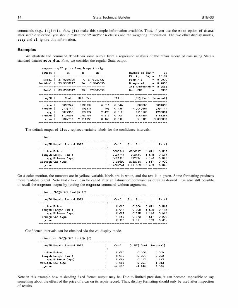
We illustrate the command diest via some output from a regression analysis of the repair record of cars using Stata’sstandard dataset auto.dta. First, we consider the regular Stata output.
. regress rep78 price length mpg foreign
Source | SS df MS Number of obs = 69
---------+------------------------------ F( 4, 64) = 10.92
Model | 27.0380695 4 6.75951737 Prob > F = 0.0000
Residual | 39.5996117 64 .618743933 R-squared = 0.4057
---------+------------------------------ Adj R-squared = 0.3686
Total | 66.6376812 68 .979965899 Root MSE = .7866
------------------------------------------------------------------------------
rep78 | Coef. Std. Err. t P>|t| [95% Conf. Interval]
---------+--------------------------------------------------------------------
price | .0000242 .0000397 0.611 0.544 -.000055 .0001035
length | .0125744 .008331 1.509 0.136 -.0040687 .0292174
mpg | .0674953 .027824 2.426 0.018 .0119106 .1230801
foreign | 1.25691 .2782758 4.517 0.000 .7009899 1.81283
_cons | -.9302744 2.011363 -0.463 0.645 -4.948433 3.087884
------------------------------------------------------------------------------
The default output of diest replaces variable labels for the confidence intervals.
. diest
------------------------------------------------------------------------------
rep78 Repair Record 1978 | Coef. Std. Err. t P>|t|
-----------------------------------------+------------------------------------
price Price | .0000242 .0000397 0.611 0.544
length Length (in.) | .0125744 .008331 1.509 0.136
mpg Mileage (mpg) | .0674953 .027824 2.426 0.018
foreign Car type | 1.25691 .2782758 4.517 0.000
_cons | -.9302744 2.011363 -0.463 0.645
------------------------------------------------------------------------------
On a color monitor, the numbers are in yellow, variable labels are in white, and the rest is in green. Some formatting producesmore readable output. Note that diest can be called after an estimation command as often as desired. It is also still possibleto recall the regress output by issuing the regress command without arguments.
. diest, fb(%9.3f) fse(%9.3f)
------------------------------------------------------------------------------
rep78 Repair Record 1978 | Coef. Std. Err. t P>|t|
-----------------------------------------+------------------------------------
price Price | 0.000 0.000 0.611 0.544
length Length (in.) | 0.013 0.008 1.509 0.136
mpg Mileage (mpg) | 0.067 0.028 2.426 0.018
foreign Car type | 1.257 0.278 4.517 0.000
_cons | -0.930 2.011 -0.463 0.645
------------------------------------------------------------------------------
Confidence intervals can be obtained via the ci display mode.
. diest, ci fb(%9.3f) fci(%9.3f)
------------------------------------------------------------------------------
rep78 Repair Record 1978 | Coef. [t 95% Conf. Interval]
-----------------------------------------+------------------------------------
price Price | 0.000 -0.000 0.000
length Length (in.) | 0.013 -0.004 0.029
mpg Mileage (mpg) | 0.067 0.012 0.123
foreign Car type | 1.257 0.701 1.813
_cons | -0.930 -4.948 3.088
------------------------------------------------------------------------------
Note in this example how misleading fixed format output may be. Due to limited precision, it can become impossible to saysomething about the effect of the price of a car on its repair record. Thus, display formating should only be used after inspectionof results.
Stata Technical Bulletin 15
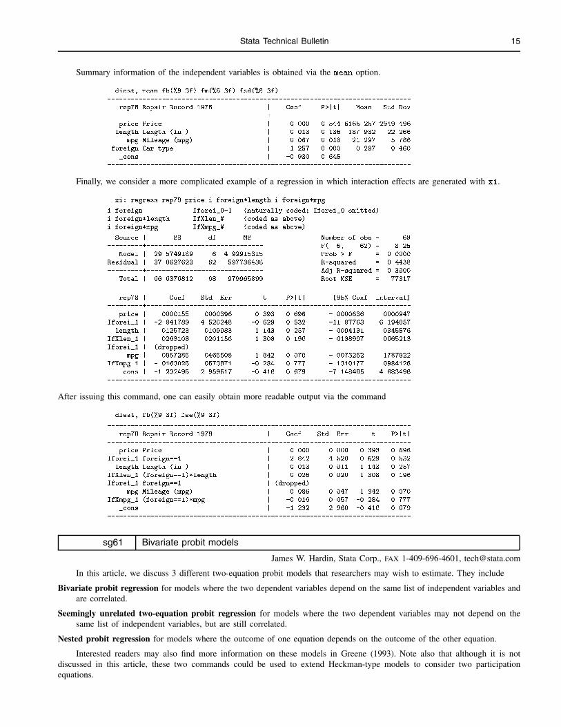
Summary information of the independent variables is obtained via the mean option.
. diest, mean fb(%9.3f) fm(%8.3f) fsd(%8.3f)
------------------------------------------------------------------------------
rep78 Repair Record 1978 | Coef. P>|t| Mean Std Dev
-----------------------------------------+------------------------------------
price Price | 0.000 0.544 6165.257 2949.496
length Length (in.) | 0.013 0.136 187.932 22.266
mpg Mileage (mpg) | 0.067 0.018 21.297 5.786
foreign Car type | 1.257 0.000 0.297 0.460
_cons | -0.930 0.645
------------------------------------------------------------------------------
Finally, we consider a more complicated example of a regression in which interaction effects are generated with xi.
. xi: regress rep78 price i.foreign*length i.foreign*mpg
i.foreign Iforei_0-1 (naturally coded; Iforei_0 omitted)
i.foreign*length IfXlen_# (coded as above)
i.foreign*mpg IfXmpg_# (coded as above)
Source | SS df MS Number of obs = 69
---------+------------------------------ F( 6, 62) = 8.25
Model | 29.5749189 6 4.92915315 Prob > F = 0.0000
Residual | 37.0627623 62 .597786488 R-squared = 0.4438
---------+------------------------------ Adj R-squared = 0.3900
Total | 66.6376812 68 .979965899 Root MSE = .77317
------------------------------------------------------------------------------
rep78 | Coef. Std. Err. t P>|t| [95% Conf. Interval]
---------+--------------------------------------------------------------------
price | .0000155 .0000396 0.393 0.696 -.0000636 .0000947
Iforei_1 | -2.841789 4.520248 -0.629 0.532 -11.87763 6.194057
length | .0125723 .0109983 1.143 0.257 -.0094131 .0345576
IfXlen_1 | .0263108 .0201156 1.308 0.196 -.0138997 .0665213
Iforei_1 | (dropped)
mpg | .0857285 .0465508 1.842 0.070 -.0073252 .1787822
IfXmpg_1 | -.0163025 .0573871 -0.284 0.777 -.1310177 .0984126
_cons | -1.232495 2.959517 -0.416 0.679 -7.148485 4.683496
------------------------------------------------------------------------------
After issuing this command, one can easily obtain more readable output via the command
. diest, fb(%9.3f) fse(%9.3f)
------------------------------------------------------------------------------
rep78 Repair Record 1978 | Coef. Std. Err. t P>|t|
-----------------------------------------+------------------------------------
price Price | 0.000 0.000 0.393 0.696
Iforei_1 foreign==1 | -2.842 4.520 -0.629 0.532
length Length (in.) | 0.013 0.011 1.143 0.257
IfXlen_1 (foreign==1)*length | 0.026 0.020 1.308 0.196
Iforei_1 foreign==1 | (dropped)
mpg Mileage (mpg) | 0.086 0.047 1.842 0.070
IfXmpg_1 (foreign==1)*mpg | -0.016 0.057 -0.284 0.777
_cons | -1.232 2.960 -0.416 0.679
------------------------------------------------------------------------------
sg61 Bivariate probit models
James W. Hardin, Stata Corp., FAX 1-409-696-4601, [email protected]
In this article, we discuss 3 different two-equation probit models that researchers may wish to estimate. They include
Bivariate probit regression for models where the two dependent variables depend on the same list of independent variables andare correlated.
Seemingly unrelated two-equation probit regression for models where the two dependent variables may not depend on thesame list of independent variables, but are still correlated.
Nested probit regression for models where the outcome of one equation depends on the outcome of the other equation.
Interested readers may also find more information on these models in Greene (1993). Note also that although it is notdiscussed in this article, these two commands could be used to extend Heckman-type models to consider two participationequations.
16 Stata Technical Bulletin STB-33
Common derivations
Formulation of the models starts with the basic two-equation system
yi1 = Xi1�+ �i1
yi2 = Xi2�+ �i2
��i1�i2
�� Bivariate Normal
��0
0
�; �
2
�I �I
�I I
��The estimation sample is all of the observations for which all of the variables in the two equations are observed in the
bivariate and seemingly unrelated models. For the nested model, the estimation sample is the sample defined by the containingequation—the contained equation is assumed to be missing for observations where the dependent variable of the containingequation is zero.
Throughout the next sections, we will use � to denote the standard normal cdf, �2 to denote the standard bivariate normalcdf, � to denote the standard normal pdf, and �2 to denote the standard bivariate normal pdf.
The bivariate and seemingly unrelated models summarize the 4 possible outcomes such that for a given observation wehave
Pi11 = P (yi1 = 1; yi2 = 1)
Pi10 = P (yi1 = 1; yi2 = 0)
Pi01 = P (yi1 = 0; yi2 = 1)
Pi00 = P (yi1 = 0; yi2 = 0)
For these two models, we have that
Pi11 = �2(xi1�1;xi2�2; �)
Pi10 = �(xi1�1)� �2(xi1�1;xi2�2; �)
Pi01 = �(xi2�2)� �2(xi1�1;xi2�2; �)
Pi00 = �2(xi1�1;xi2�2; �)� �(xi1�1)� �(xi2�2)
where the bivariate probit has Xi1 = Xi2 for all i.
For the nested model, we have thatPi11 = �2(xi1�1;xi2�2; �)
Pi10 = �2(�xi1�1;xi2�2;��)
Pi01 = �(�xi2�2)
Pi00 = �(�xi2�2)
where equation 1 is nested within equation 2; that is, the outcome for y2 is only available when y1 6= 0.
Implementation
In fact, all of these models may be implemented with only one command, but two are provided. The only necessarycommand is suprob that takes two equations as arguments, but we provide biprob as a convenience so that you are not requiredto set up the appropriate equations and may instead use mvreg-type syntax.
The syntax for suprob and biprob are
suprob eq1 eq2�, robust cluster(cluster varname) score(score1 score2) nochi
nested level(#) maximize options�
biprob depvar1 depvar2�varlist
� �, robust cluster(cluster varname) score(score1 score2) nochi
level(#) maximize options�
Stata Technical Bulletin 17
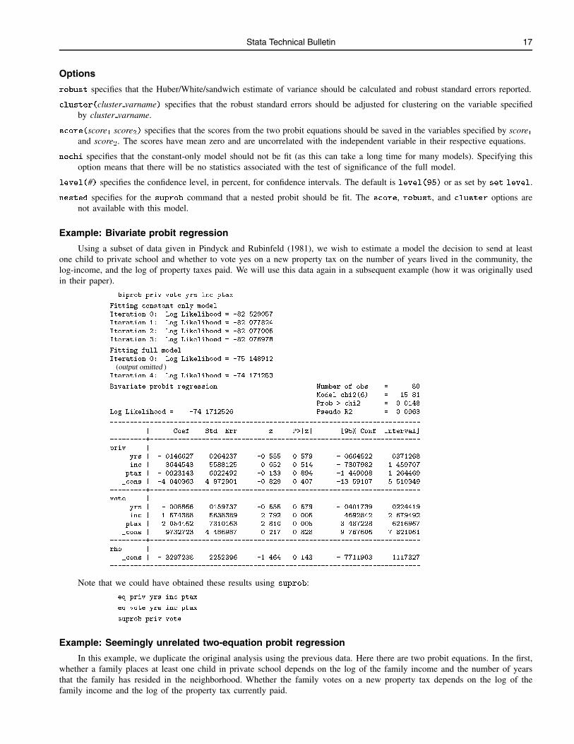
Options
robust specifies that the Huber/White/sandwich estimate of variance should be calculated and robust standard errors reported.
cluster(cluster varname) specifies that the robust standard errors should be adjusted for clustering on the variable specifiedby cluster varname.
score(score1 score2) specifies that the scores from the two probit equations should be saved in the variables specified by score1and score2. The scores have mean zero and are uncorrelated with the independent variable in their respective equations.
nochi specifies that the constant-only model should not be fit (as this can take a long time for many models). Specifying thisoption means that there will be no statistics associated with the test of significance of the full model.
level(#) specifies the confidence level, in percent, for confidence intervals. The default is level(95) or as set by set level.
nested specifies for the suprob command that a nested probit should be fit. The score, robust, and cluster options arenot available with this model.
Example: Bivariate probit regression
Using a subset of data given in Pindyck and Rubinfeld (1981), we wish to estimate a model the decision to send at leastone child to private school and whether to vote yes on a new property tax on the number of years lived in the community, thelog-income, and the log of property taxes paid. We will use this data again in a subsequent example (how it was originally usedin their paper).
. biprob priv vote yrs inc ptax
Fitting constant only model
Iteration 0: Log Likelihood = -82.529057
Iteration 1: Log Likelihood = -82.077824
Iteration 2: Log Likelihood = -82.077005
Iteration 3: Log Likelihood = -82.076978
Fitting full model
Iteration 0: Log Likelihood = -75.148912
(output omitted )Iteration 4: Log Likelihood = -74.171253
Bivariate probit regression Number of obs = 80
Model chi2(6) = 15.81
Prob > chi2 = 0.0148
Log Likelihood = -74.1712526 Pseudo R2 = 0.0963
------------------------------------------------------------------------------
| Coef. Std. Err. z P>|z| [95% Conf. Interval]
---------+--------------------------------------------------------------------
priv |
yrs | -.0146627 .0264237 -0.555 0.579 -.0664522 .0371268
inc | .3644543 .5588125 0.652 0.514 -.7307982 1.459707
ptax | -.0923143 .6922492 -0.133 0.894 -1.449098 1.264469
_cons | -4.040363 4.872901 -0.829 0.407 -13.59107 5.510349
---------+--------------------------------------------------------------------
vote |
yrs | -.008866 .0159737 -0.555 0.579 -.0401739 .0224419
inc | 1.574388 .5638389 2.792 0.005 .4692842 2.679492
ptax | -2.054462 .7310163 -2.810 0.005 -3.487228 -.6216967
_cons | -.9732723 4.486987 -0.217 0.828 -9.767606 7.821061
---------+--------------------------------------------------------------------
rho |
_cons | -.3297288 .2252396 -1.464 0.143 -.7711903 .1117327
------------------------------------------------------------------------------
Note that we could have obtained these results using suprob:
. eq priv yrs inc ptax
. eq vote yrs inc ptax
. suprob priv vote
Example: Seemingly unrelated two-equation probit regression
In this example, we duplicate the original analysis using the previous data. Here there are two probit equations. In the first,whether a family places at least one child in private school depends on the log of the family income and the number of yearsthat the family has resided in the neighborhood. Whether the family votes on a new property tax depends on the log of thefamily income and the log of the property tax currently paid.
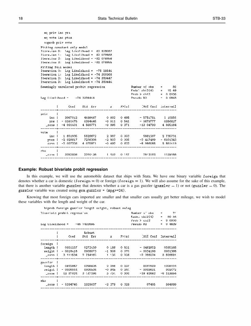
18 Stata Technical Bulletin STB-33
. eq priv inc yrs
. eq vote inc ptax
. suprob priv vote
Fitting constant only model
Iteration 0: Log Likelihood = -82.529057
Iteration 1: Log Likelihood = -82.078668
Iteration 2: Log Likelihood = -82.076956
Iteration 3: Log Likelihood = -82.076955
Fitting full model
Iteration 0: Log Likelihood = -75.29544
Iteration 1: Log Likelihood = -74.350968
Iteration 2: Log Likelihood = -74.333447
Iteration 3: Log Likelihood = -74.333444
Seemingly unrelated probit regression Number of obs = 80
Model chi2(4) = 15.49
Prob > chi2 = 0.0038
Log Likelihood = -74.3334444 Pseudo R2 = 0.0943
------------------------------------------------------------------------------
| Coef. Std. Err. z P>|z| [95% Conf. Interval]
---------+--------------------------------------------------------------------
priv |
inc | .3067012 .4499467 0.682 0.495 -.5751781 1.18858
yrs | -.0161475 .0264445 -0.611 0.541 -.0679777 .0356827
_cons | -4.091401 4.569771 -0.895 0.371 -13.04799 4.865184
---------+--------------------------------------------------------------------
vote |
inc | 1.651935 .5529672 2.987 0.003 .5681397 2.735731
ptax | -2.028817 .7238308 -2.803 0.005 -3.447499 -.6101343
_cons | -2.007338 4.075971 -0.492 0.622 -9.996095 5.981419
---------+--------------------------------------------------------------------
rho |
_cons | -.3252008 .2240436 -1.452 0.147 -.7643183 .1139166
------------------------------------------------------------------------------
Example: Robust bivariate probit regression
In this example, we will use the automobile dataset that ships with Stata. We have one binary variable foreign thatdenotes whether a car is domestic (foreign = 0) or foreign (foreign = 1). We will also assume for the sake of this example,that there is another variable guzzler that denotes whether a car is a gas guzzler (guzzler = 1) or not (guzzler = 0). Theguzzler variable was created using gen guzzler = (mpg>=24).
Knowing that most foreign cars imported are smaller and that smaller cars usually get better mileage, we wish to modelthese variables with the length and weight of the car.
. biprob foreign guzzler length weight, robust nolog
Bivariate probit regression Number of obs = 74
Model chi2(4) = 80.56
Prob > chi2 = 0.0000
Log Likelihood = -46.7432695 Pseudo R2 = 0.4629
------------------------------------------------------------------------------
| Robust
| Coef. Std. Err. z P>|z| [95% Conf. Interval]
---------+--------------------------------------------------------------------
foreign |
length | .0051157 .0272459 0.188 0.851 -.0482852 .0585166
weight | -.0016416 .0009073 -1.809 0.070 -.0034198 .0001366
_cons | 3.111534 2.754162 1.130 0.259 -2.286524 8.509591
---------+--------------------------------------------------------------------
guzzler |
length | -.0622867 .0298606 -2.086 0.037 .0037609 .1208124
weight | -.0008044 .0008508 -0.945 0.344 -.0008631 .002472
_cons | 12.87024 3.447198 3.734 0.000 -19.62662 -6.113856
---------+--------------------------------------------------------------------
rho |
_cons | -.5294745 .2323637 -2.279 0.023 .07405 .984899
------------------------------------------------------------------------------
Stata Technical Bulletin 19
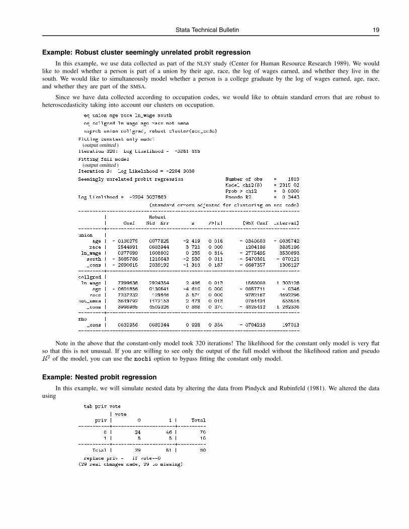
Example: Robust cluster seemingly unrelated probit regression
In this example, we use data collected as part of the NLSY study (Center for Human Resource Research 1989). We wouldlike to model whether a person is part of a union by their age, race, the log of wages earned, and whether they live in thesouth. We would like to simultaneously model whether a person is a college graduate by the log of wages earned, age, race,and whether they are part of the SMSA.
Since we have data collected according to occupation codes, we would like to obtain standard errors that are robust toheteroscedasticity taking into account our clusters on occupation.
. eq union age race ln_wage south
. eq collgrad ln_wage age race not_smsa
. suprob union collgrad, robust cluster(occ_code)
Fitting constant only model
(output omitted )Iteration 320: Log Likelihood = -3361.815
Fitting full model
(output omitted )Iteration 3: Log Likelihood = -2204.3038
Seemingly unrelated probit regression Number of obs = 1819
Model chi2(8) = 2315.02
Prob > chi2 = 0.0000
Log Likelihood = -2204.3037683 Pseudo R2 = 0.3443
(standard errors adjusted for clustering on occ_code)
------------------------------------------------------------------------------
| Robust
| Coef. Std. Err. z P>|z| [95% Conf. Interval]
---------+--------------------------------------------------------------------
union |
age | -.0188275 .0077825 -2.419 0.016 -.0340808 -.0035742
race | .2544691 .0683944 3.721 0.000 .1204186 .3885196
ln_wage | .0377699 .1608802 0.235 0.814 -.2775495 .3530893
south | -.3085786 .1216643 -2.536 0.011 -.5470361 -.070121
_cons | -.2690615 .2039192 -1.319 0.187 -.6687357 .1306127
---------+--------------------------------------------------------------------
collgrad |
ln_wage | .7299636 .2924354 2.496 0.013 .1568008 1.303126
age | -.0601856 .0130541 -4.610 0.000 -.0857711 -.0346
race | -.7237232 .129846 -5.574 0.000 -.9782167 -.4692296
not_smsa | .3649792 .1472153 2.479 0.013 .0764424 .653516
_cons | .3998985 .4502326 0.888 0.374 -.4825412 1.282338
---------+--------------------------------------------------------------------
rho |
_cons | .0632956 .0682244 0.928 0.354 -.0704218 .197013
------------------------------------------------------------------------------
Note in the above that the constant-only model took 320 iterations! The likelihood for the constant only model is very flatso that this is not unusual. If you are willing to see only the output of the full model without the likelihood ration and pseudoR2 of the model, you can use the nochi option to bypass fitting the constant only model.
Example: Nested probit regression
In this example, we will simulate nested data by altering the data from Pindyck and Rubinfeld (1981). We altered the datausing
. tab priv vote
| vote
priv | 0 1 | Total
-----------+----------------------+----------
0 | 24 46 | 70
1 | 5 5 | 10
-----------+----------------------+----------
Total | 29 51 | 80
. replace priv = . if vote==0
(29 real changes made, 29 to missing)
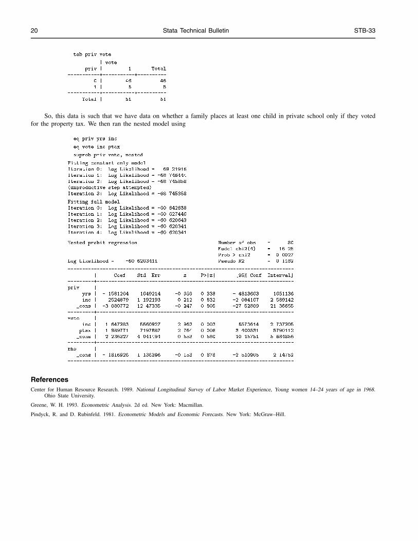
20 Stata Technical Bulletin STB-33
. tab priv vote
| vote
priv | 1 | Total
-----------+-----------+----------
0 | 46 | 46
1 | 5 | 5
-----------+-----------+----------
Total | 51 | 51
So, this data is such that we have data on whether a family places at least one child in private school only if they votedfor the property tax. We then ran the nested model using
. eq priv yrs inc
. eq vote inc ptax
. suprob priv vote, nested
Fitting constant only model
Iteration 0: Log Likelihood = -69.21916
Iteration 1: Log Likelihood = -68.746444
Iteration 2: Log Likelihood = -68.745858
(unproductive step attempted)
Iteration 3: Log Likelihood = -68.745858
Fitting full model
Iteration 0: Log Likelihood = -60.842838
Iteration 1: Log Likelihood = -60.627446
Iteration 2: Log Likelihood = -60.620643
Iteration 3: Log Likelihood = -60.620341
Iteration 4: Log Likelihood = -60.620341
Nested probit regression Number of obs = 80
Model chi2(4) = 16.25
Prob > chi2 = 0.0027
Log Likelihood = -60.6203411 Pseudo R2 = 0.1182
------------------------------------------------------------------------------
| Coef. Std. Err. z P>|z| [95% Conf. Interval]
---------+--------------------------------------------------------------------
priv |
yrs | -.1581264 .1649214 -0.959 0.338 -.4813663 .1651136
inc | .2524879 1.192193 0.212 0.832 -2.084167 2.589142
_cons | -3.080772 12.47335 -0.247 0.805 -27.52809 21.36655
---------+--------------------------------------------------------------------
vote |
inc | 1.647283 .5560927 2.962 0.003 .5573614 2.737205
ptax | -1.989771 .7197887 -2.764 0.006 -3.400531 -.5790112
_cons | -2.236327 4.041494 -0.553 0.580 -10.15751 5.684856
---------+--------------------------------------------------------------------
rho |
_cons | -.1816928 1.188396 -0.153 0.878 -2.510905 2.14752
------------------------------------------------------------------------------
ReferencesCenter for Human Resource Research. 1989. National Longitudinal Survey of Labor Market Experience, Young women 14–24 years of age in 1968.
Ohio State University.
Greene, W. H. 1993. Econometric Analysis. 2d ed. New York: Macmillan.
Pindyck, R. and D. Rubinfeld. 1981. Econometric Models and Economic Forecasts. New York: McGraw–Hill.
Stata Technical Bulletin 21
sg62 Hildreth–Houck random coefficients model
James W. Hardin, Stata Corp., FAX 1-409-696-4601, [email protected]
In Stata 5.0, we released a collection of panel data routines for analyzing cross-sectional time-series data. One of the newcommands, xtgls, will estimate a linear model in the presence of heteroscedasticity, cross-sectional correlation, and within-panelautocorrelation. The command actually includes 9 different models depending on which options are chosen and will report eitherthe GLS or OLS results. However, all of the models that the xtgls command will estimate assume that the parameter vector isconstant for the panels.
In random coefficient models, we wish to treat the parameter vector as a realization in each panel of a stochastic process.
Remarks
Interested readers should see Greene (1993) for information on this and other panel data models. In a random coefficientmodel, the parameter heterogeneity is viewed due to stochastic variation. Assume that we write
yi = Xi�i + �i
where i = 1; : : : ;m, and �i is the coefficient vector (k � 1) for the ith cross-sectional unit such that
�i = �+ �i E(�i) = 0 E(�i�0
i) = �
where our goal is to find b� and b�.
The derivation of the estimator assumes that the cross-sectional specific coefficient vector �i is the outcome of a randomprocess with mean vector � and covariance matrix �.
yi = Xi�i + �i = Xi(�+ �i) + �i = Xi�+ (Xi�i + �i) = Xi�+ !i
where E(!i) = 0 and
E(!i!0
i) = E((Xi�i + �i)(Xi�i + �i)0) = E(�i�
0
i) +XiE(�i�0
i)X0
i = �2i I+Xi�X
0
i =�i
The covariance matrix for the panel-specific coefficient estimator �i can then be written
Vi + � = (X0
iXi)�1X
0
i�iXi(X0
iXi)�1 where Vi = �
2i (X
0
iX)�1
We may then compute a weighted average of the panel-specific coefficient estimates as
b� =
mXi=1
Wi�i where Wi =
(mXi=1
[�+Vi]�1
)�1
[�+Vi]�1
such that the resulting GLS estimator is a matrix-weighted average of the panel-specific (OLS) estimators.
In order to calculate the above estimator b� for the unknown � and Vi parameters, we may use the two-step approachsuggested by Swamy (1970, 1971):
b�i = OLS panel� speci�c estimator
bVi =b�i 0b�ini � k
�� =1
m
mXi=1
b�ib� =
1
m� 1
mXi=1
b�ib�i 0 �m�� ��
!�
1
m
mXi=1
bVi
The two-step procedure begins with the usual OLS estimate of �. With an estimate of �, we may proceed by (1) obtainingestimates of bVi and b� (and, thus, cWi) and then (2) obtain an updated estimate of �.
22 Stata Technical Bulletin STB-33
Swamy (1970, 1971) further points out that the matrix b� may not be positive definite and that since the second term is oforder 1=(mT ), it is negligible in large samples. A simple and asymptotically expedient solution is to simply drop this secondterm and instead use b� =
1
m� 1
mXi=1
b�ib�0i �m�� ��
!
As a test of the model, we may look at the difference between the OLS estimate of � ignoring the panel structure of thedata and the matrix-weighted average of the panel-specific OLS estimators. The test statistic suggested by Swamy (1970, 1971)is given by
�2k(m�1) =
mXi=1
[b�i � ���
]0 bV�1
i [b�i � ���
] where ���
=
"mXi=1
bV�1i
#�1 mX
i=1
bV�1ib�i
Johnston (1984) has shown that the test is algebraically equivalent to testing
H0 : �1 = �2 = � � � = �m
in the generalized (groupwise heteroscedastic) xtgls model where V is block diagonal with ith diagonal element �i.
xtrchh is an implementation of the random coefficients model (including the test of parameter constancy) with syntaxgiven by
xtrchh depvar�varlist
� �if exp
� �in range
� �, i(varnamei) t(varnamet) level(#)
�Options
i(varname) specifies the variable that contains the unit to which the observation belongs. You can specify the i() option thefirst time you estimate or use the iis command to set i() beforehand. After that, Stata will remember the variable’sidentity. See [R] xt in the Stata 5.0 Reference Manual.
t(varname) specifies the variable that contains the time at which the observation was made. You can specify the t() optionthe first time you estimate or use the tis command to set t() beforehand. After that, Stata will remember the variable’sidentity.
level(#) specifies the confidence level, in percent, for confidence intervals. The default is level(95) or as set by set level.
Example
Greene (1993, 445) reprints data in a classic study of investment demand by Grunfeld and Griliches (1960). In the Statamanual, we use this data to illustrate many of the possible models that may be estimated with the xtgls command. While themodels included in the xtgls command offer considerable flexibility, they all assume that there is no parameter variation acrossfirms (the cross-sectional units).
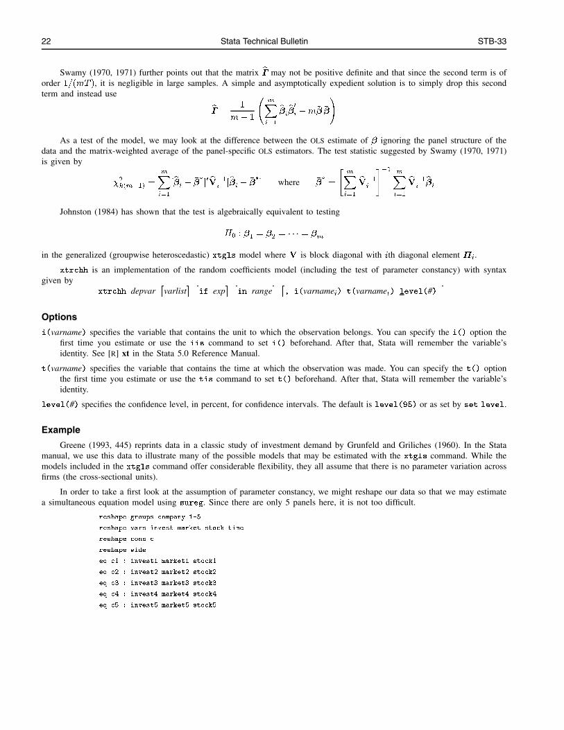
In order to take a first look at the assumption of parameter constancy, we might reshape our data so that we may estimatea simultaneous equation model using sureg. Since there are only 5 panels here, it is not too difficult.
. reshape groups company 1-5
. reshape vars invest market stock time
. reshape cons c
. reshape wide
. eq c1 : invest1 market1 stock1
. eq c2 : invest2 market2 stock2
. eq c3 : invest3 market3 stock3
. eq c4 : invest4 market4 stock4
. eq c5 : invest5 market5 stock5
Stata Technical Bulletin 23
. sureg c1 c2 c3 c4 c5
Equation Obs Parms RMSE "R-sq" F P
------------------------------------------------------------------
c1 20 3 91.78166 0.9214 111.0618 0.0000
c2 20 3 13.27856 0.9136 88.06545 0.0000
c3 20 3 27.88272 0.7053 19.92612 0.0000
c4 20 3 10.21312 0.7444 25.13699 0.0000
c5 20 3 102.3053 0.4403 6.361697 0.0027
------------------------------------------------------------------------------
| Coef. Std. Err. t P>|t| [95% Conf. Interval]
---------+--------------------------------------------------------------------
c1 |
market1 | .120493 .0234601 5.136 0.000 .0738481 .1671379
stock1 | .3827462 .0355419 10.769 0.000 .3120793 .453413
_cons | -162.3641 97.03215 -1.673 0.098 -355.29 30.56183
---------+--------------------------------------------------------------------
c2 |
market2 | .0695456 .0183279 3.795 0.000 .0331048 .1059864
stock2 | .3085445 .028053 10.999 0.000 .2527677 .3643213
_cons | .5043113 12.48742 0.040 0.968 -24.32402 25.33264
---------+--------------------------------------------------------------------
c3 |
market3 | .0372914 .0133012 2.804 0.006 .010845 .0637379
stock3 | .130783 .0239163 5.468 0.000 .083231 .178335
_cons | -22.43892 27.67879 -0.811 0.420 -77.47177 32.59393
---------+--------------------------------------------------------------------
c4 |
market4 | .0570091 .0123241 4.626 0.000 .0325055 .0815127
stock4 | .0415065 .0446894 0.929 0.356 -.047348 .130361
_cons | 1.088878 6.788627 0.160 0.873 -12.40873 14.58649
---------+--------------------------------------------------------------------
c5 |
market5 | .1014782 .0594213 1.708 0.091 -.0166671 .2196236
stock5 | .3999914 .1386127 2.886 0.005 .1243922 .6755905
_cons | 85.42324 121.3481 0.704 0.483 -155.8493 326.6957
------------------------------------------------------------------------------
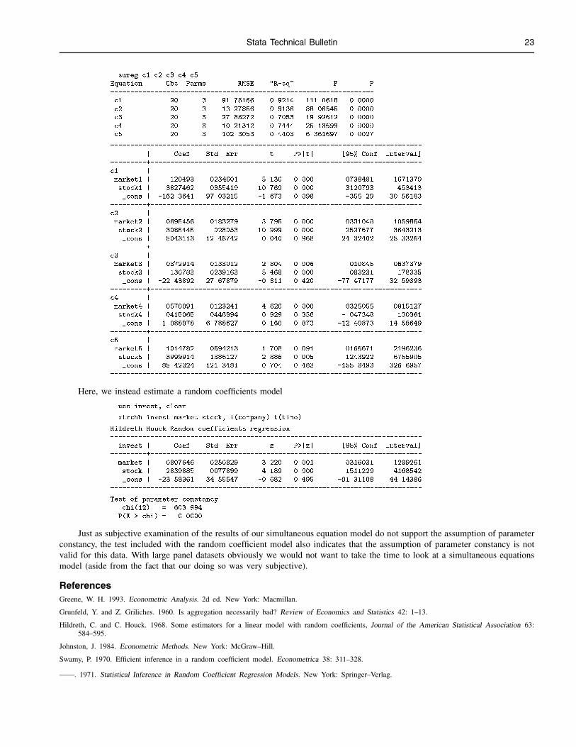
Here, we instead estimate a random coefficients model
. use invest, clear
. xtrchh invest market stock, i(company) t(time)
Hildreth-Houck Random coefficients regression
------------------------------------------------------------------------------
invest | Coef. Std. Err. z P>|z| [95% Conf. Interval]
---------+--------------------------------------------------------------------
market | .0807646 .0250829 3.220 0.001 .0316031 .1299261
stock | .2839885 .0677899 4.189 0.000 .1511229 .4168542
_cons | -23.58361 34.55547 -0.682 0.495 -91.31108 44.14386
------------------------------------------------------------------------------
Test of parameter constancy
chi(12) = 603.994
P(X > chi) = 0.0000
Just as subjective examination of the results of our simultaneous equation model do not support the assumption of parameterconstancy, the test included with the random coefficient model also indicates that the assumption of parameter constancy is notvalid for this data. With large panel datasets obviously we would not want to take the time to look at a simultaneous equationsmodel (aside from the fact that our doing so was very subjective).
ReferencesGreene, W. H. 1993. Econometric Analysis. 2d ed. New York: Macmillan.
Grunfeld, Y. and Z. Griliches. 1960. Is aggregation necessarily bad? Review of Economics and Statistics 42: 1–13.
Hildreth, C. and C. Houck. 1968. Some estimators for a linear model with random coefficients, Journal of the American Statistical Association 63:584–595.
Johnston, J. 1984. Econometric Methods. New York: McGraw–Hill.
Swamy, P. 1970. Efficient inference in a random coefficient model. Econometrica 38: 311–328.
——. 1971. Statistical Inference in Random Coefficient Regression Models. New York: Springer–Verlag.
24 Stata Technical Bulletin STB-33
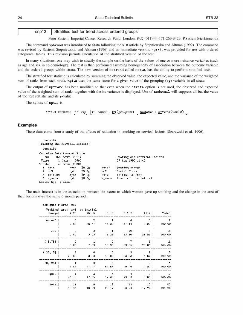
snp12 Stratified test for trend across ordered groups
Peter Sasieni, Imperial Cancer Research Fund, London, FAX (011)-44-171-269-3429, [email protected]
The command nptrend was introduced to Stata following the STB article by Stepniewska and Altman (1992). The commandwas revised by Sasieni, Stepniewska, and Altman (1996) and an immediate version, nptri, was provided for use with orderedcategorical tables. This revision permits calculation of the stratified version of the test.
In many situations, one may wish to stratify the sample on the basis of the values of one or more nuisance variables (suchas age and sex in epidemiology). The test is then performed assuming homogeneity of association between the outcome variableand the ordered groups within strata. The new version of nptrend called npt s, has the ability to perform stratified tests.
The stratified test statistic is calculated by summing the observed value, the expected value, and the variance of the weightedsum of ranks from each strata. npt s uses the same score for a given value of the grouping (by) variable in all strata.
The output of nptrend has been modified so that even when the strata option is not used, the observed and expectedvalue of the weighted sum of ranks together with the its variance is displayed. Use of nodetail will suppress all but the valueof the test statistic and its p-value.
The syntax of npt s is
npt s varname�if exp
� �in range
�, by(groupvar)
�nodetail strata(varlist)
�Examples
These data come from a study of the effects of reduction in smoking on cervical lesions (Szarewski et al. 1996).
. use stb2
(Smoking and cervical lesions)
. describe
Contains data from stb2.dta
Obs: 82 (max= 2021) Smoking and cervical lesions
Vars: 4 (max= 999) 27 Aug 1996 14:42
Width: 4 (max= 2000)
1. quit byte %8.0g quit2 Smoking change
2. sc3 byte %9.0g sc3 Social Class
3. init_sm byte %9.0g init2 Initial No./day
4. r_area byte %9.0g r_area Area: rel. to initial
Sorted by: r_area
The main interest is in the association between the extent to which women gave up smoking and the change in the area oftheir lesions over the same 6 month period.
. tab quit r_area, row
Smoking| Area: rel. to initial
change| <.25 .25-.5 .5-.8 .8-1.2 >1.2 | Total
-----------+-------------------------------------------------------+----------
unconf | 0 2 1 4 0 | 7
| 0.00 28.57 14.29 57.14 0.00 | 100.00
-----------+-------------------------------------------------------+----------
>75 | 0 0 1 12 6 | 19
| 0.00 0.00 5.26 63.16 31.58 | 100.00
-----------+-------------------------------------------------------+----------
(.5,75] | 0 1 2 7 3 | 13
| 0.00 7.69 15.38 53.85 23.08 | 100.00
-----------+-------------------------------------------------------+----------
(.25,.5] | 3 0 6 5 1 | 15
| 20.00 0.00 40.00 33.33 6.67 | 100.00
-----------+-------------------------------------------------------+----------
(0,.25] | 1 3 6 1 0 | 11
| 9.09 27.27 54.55 9.09 0.00 | 100.00
-----------+-------------------------------------------------------+----------
quit | 7 3 3 4 0 | 17
| 41.18 17.65 17.65 23.53 0.00 | 100.00
-----------+-------------------------------------------------------+----------
Total| 11 9 19 33 10 | 82
| 13.41 10.98 23.17 40.24 12.20 | 100.00
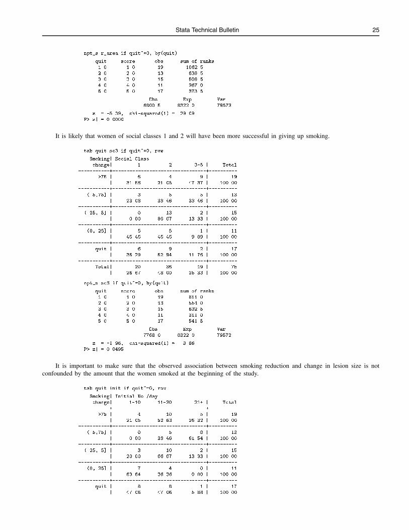
Stata Technical Bulletin 25
. npt_s r_area if quit~=0, by(quit)
quit score obs sum of ranks
1.0 1.0 19 1062.5
2.0 2.0 13 638.5
3.0 3.0 15 508.5
4.0 4.0 11 267.0
5.0 5.0 17 373.5
Obs Exp Var
6800.5 8322.0 79572
z = -5.39, chi-squared(1) = 29.09
P>|z| = 0.0000
It is likely that women of social classes 1 and 2 will have been more successful in giving up smoking.
. tab quit sc3 if quit~=0, row
Smoking| Social Class
change| 1 2 3-5 | Total
-----------+---------------------------------+----------
>75 | 6 4 9 | 19
| 31.58 21.05 47.37 | 100.00
-----------+---------------------------------+----------
(.5,75] | 3 5 5 | 13
| 23.08 38.46 38.46 | 100.00
-----------+---------------------------------+----------
(.25,.5] | 0 13 2 | 15
| 0.00 86.67 13.33 | 100.00
-----------+---------------------------------+----------
(0,.25] | 5 5 1 | 11
| 45.45 45.45 9.09 | 100.00
-----------+---------------------------------+----------
quit | 6 9 2 | 17
| 35.29 52.94 11.76 | 100.00
-----------+---------------------------------+----------
Total| 20 36 19 | 75
| 26.67 48.00 25.33 | 100.00
. npt_s sc3 if quit~=0, by(quit)
quit score obs sum of ranks
1.0 1.0 19 811.0
2.0 2.0 13 554.0
3.0 3.0 15 632.5
4.0 4.0 11 311.0
5.0 5.0 17 541.5
Obs Exp Var
7768.0 8322.0 79572
z = -1.96, chi-squared(1) = 3.86
P>|z| = 0.0495
It is important to make sure that the observed association between smoking reduction and change in lesion size is notconfounded by the amount that the women smoked at the beginning of the study.
. tab quit init if quit~=0, row
Smoking| Initial No./day
change| 1-10 11-20 21+ | Total
-----------+---------------------------------+----------
>75 | 4 10 5 | 19
| 21.05 52.63 26.32 | 100.00
-----------+---------------------------------+----------
(.5,75] | 0 5 8 | 13
| 0.00 38.46 61.54 | 100.00
-----------+---------------------------------+----------
(.25,.5] | 3 10 2 | 15
| 20.00 66.67 13.33 | 100.00
-----------+---------------------------------+----------
(0,.25] | 7 4 0 | 11
| 63.64 36.36 0.00 | 100.00
-----------+---------------------------------+----------
quit | 8 8 1 | 17
| 47.06 47.06 5.88 | 100.00
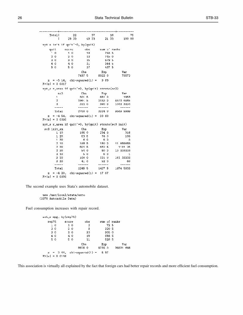
26 Stata Technical Bulletin STB-33
-----------+---------------------------------+----------
Total| 22 37 16 | 75
| 29.33 49.33 21.33 | 100.00
. npt_s init if quit~=0, by(quit)
quit score obs sum of ranks
1.0 1.0 19 793.5
2.0 2.0 13 745.0
3.0 3.0 15 579.5
4.0 4.0 11 244.5
5.0 5.0 17 487.5
Obs Exp Var
7437.5 8322.0 79572
z = -3.14, chi-squared(1) = 9.83
P>|z| = 0.0017
. npt_s r_area if quit~=0, by(quit) strata(sc3)
sc3 Obs Exp Var
1 504.5 651.0 1953
2 1964.5 2183.0 6573.6665
3 311.0 390.0 1043.3334
----- ------ ------ ------
Total 2780.0 3224.0 9569.9999
z = -4.54, chi-squared(1) = 20.60
P>|z| = 0.0000
. npt_s r_area if quit~=0, by(quit) strata(sc3 init)
sc3 init_sm Obs Exp Var
1 10 195.0 234.0 316
1 20 53.5 76.0 100
1 30 6.0 6.0 0
2 10 189.5 190.0 41.666668
2 20 601.5 682.5 1181.25
2 30 54.0 60.0 13.333333
3 10 5.0 6.0 1
3 20 100.0 121.0 161.33333
3 30 41.0 52.0 60
----- ------ ------ ------
Total 1245.5 1427.5 1874.5833
z = -4.20, chi-squared(1) = 17.67
P>|z| = 0.0000
The second example uses Stata’s automobile dataset.
. use /usr/local/stata/auto
(1978 Automobile Data)
Fuel consumption increases with repair record.
. npt_s mpg, by(rep78)
rep78 score obs sum of ranks
1.0 1.0 2 72.5
2.0 2.0 8 220.5
3.0 3.0 30 905.0
4.0 4.0 18 688.5
5.0 5.0 11 528.5
Obs Exp Var
8625.0 8225.0 26821.666
z = 2.44, chi-squared(1) = 5.97
P>|z| = 0.0146
This association is virtually all explained by the fact that foreign cars had better repair records and more efficient fuel consumption.

Stata Technical Bulletin 27
. npt_s mpg if foreign==0, by(rep78)
rep78 score obs sum of ranks
1.0 1.0 2 60.0
2.0 2.0 8 188.5
3.0 3.0 27 648.5
4.0 4.0 9 184.0
5.0 5.0 2 95.0
Obs Exp Var
3593.5 3552.5 6463.9165
z = 0.51, chi-squared(1) = 0.26
P>|z| = 0.6101
. npt_s mpg if foreign==1, by(rep78)
rep78 score obs sum of ranks
3.0 3.0 3 28.5
4.0 4.0 9 102.0
5.0 5.0 9 100.5
Obs Exp Var
996.0 990.0 396
z = 0.30, chi-squared(1) = 0.09
P>|z| = 0.7630
. npt_s mpg, by(rep78) strata(foreign)
foreign Obs Exp Var
0 3593.5 3552.5 6463.9165
1 996.0 990.0 396
----- ------ ------ ------
Total 4589.5 4542.5 6859.9165
z = 0.57, chi-squared(1) = 0.32
P>|z| = 0.5704
This can be illustrated using the dotplot graphically as follows.
. gen for = foreign
. dotplot mpg, by(rep78) s([for]) center
Mil
ea
ge
(m
pg
)
Repair Record 19781 2 3 4 5
12
41
0
0
0
00
0 0
0
0 0
0 0
0 00
0 00
0 00 0 0 0 0 0 0
0 0 00 0 10 01
01
00
0 000
0 0
0 10
1 11
1 1 1
1 0
1
1 11 1
1
01
01 1
1
Figure 1
ReferencesStepniewska, K. A. and D. G. Altman. 1992. snp4: Non-parametric test for trend across ordered groups. Stata Technical Bulletin 9: 21–22.
Sasieni, P. D., K. A. Stepniewska, and D. G. Altman. 1996. snp11: Test for trend across ordered groups revisited. Stata Technical Bulletin 32: 27–29.

28 Stata Technical Bulletin STB-33
STB categories and insert codes
Inserts in the STB are presently categorized as follows:
General Categories:an announcements ip instruction on programmingcc communications & letters os operating system, hardware, &dm data management interprogram communicationdt datasets qs questions and suggestionsgr graphics tt teachingin instruction zz not elsewhere classified
Statistical Categories:sbe biostatistics & epidemiology ssa survival analysissed exploratory data analysis ssi simulation & random numberssg general statistics sss social science & psychometricssmv multivariate analysis sts time-series, econometricssnp nonparametric methods svy survey samplesqc quality control sxd experimental designsqv analysis of qualitative variables szz not elsewhere classifiedsrd robust methods & statistical diagnostics
In addition, we have granted one other prefix, crc, to the manufacturers of Stata for their exclusive use.
International Stata Distributors
International Stata users may also order subscriptions to the Stata Technical Bulletin from our International Stata Distributors.
Company: Applied Statistics & Company: Smit ConsultSystems Consultants Address: Scheidingstraat 1
Address: P.O. Box 1169 Postbox 220Nazerath-Ellit 17100, Israel 5150 AE Drunen
Phone: +972 6554254 NetherlandsFax: +972 6554254 Phone: +31 416-378 125
Email: [email protected] Fax: +31 416-378 385Countries served: Israel Email: [email protected]
Countries served: Netherlands
Company: Dittrich & Partner Consulting Company: Timberlake ConsultantsAddress: Prinzenstrasse 2 Address: 47 Hartfield Crescent
D-42697 Solingen West WickhamGermany Kent BR4 9DW U.K.
Phone: +49 212-3390 99 Phone: +44 181 462 0495Fax: +49 212-3390 90 Fax: +44 181 462 0493
Email: available soon Email: [email protected] served: Austria, Germany, Italy Countries served: Ireland, U.K.
Company: Metrika Consulting Company: Timberlake ConsultantsAddress: Roslagsgatan 15 Satellite Office
113 55 Stockholm Address: Praceta do Comercio,Sweden N�13–9� Dto. Quinta Grande
Phone: +46-708-163128 2720 Alfragide PortugalFax: +46-8-6122383 Phone: +351 (01) 4719337
Email: [email protected] Telemovel: 0931 62 7255Countries served: Baltic States, Denmark, Finland, Email: [email protected]
Iceland, Norway, Sweden Countries served: Portugal
Company: Ritme InformatiqueAddress: 34 boulevard Haussmann
75009 ParisFrance
Phone: +33 1 42 46 00 42Fax: +33 1 42 46 00 33
Email: [email protected] served: Belgium, France,
Luxembourg, Switzerland