TATA July 2000 ECHNICAL STB-56 ULLETIN · one character for b yte, i nt, l ong, f loat and d ouble....
52
STATA July 2000 TECHNICAL STB-56 BULLETIN A publication to promote communication among Stata users Editor Associate Editors H. Joseph Newton Nicholas J. Cox, University of Durham Department of Statistics Joanne M. Garrett, University of North Carolina Texas A & M University Marcello Pagano, Harvard School of Public Health College Station, Texas 77843 J. Patrick Royston, UK Medical Research Council 979-845-3142 Jeroen Weesie, Utrecht University 979-845-3144 FAX [email protected] EMAIL Subscriptions are available from StataCorporation, email [email protected], telephone 979-696-4600 or 800-STATAPC, fax 979-696-4601. Current subscription prices are posted at www.stata.com/bookstore/stb.html. Previous Issues are available individually from StataCorp. See www.stata.com/bookstore/stbj.html for details. Submissions to the STB, including submissions to the supporting files (programs, datasets, and help files), are on a nonexclusive, free-use basis. In particular, the author grants to StataCorp the nonexclusive right to copyright and distribute the material in accordance with the Copyright Statement below. The author also grants to StataCorp the right to freely use the ideas, including communication of the ideas to other parties, even if the material is never published in the STB. Submissions should be addressed to the Editor. Submission guidelines can be obtained from either the editor or StataCorp. Copyright Statement. The Stata Technical Bulletin (STB) and the contents of the supporting files (programs, datasets, and help files) are copyright c by StataCorp. The contents of the supporting files (programs, datasets, and help files), may be copied or reproduced by any means whatsoever, in whole or in part, as long as any copy or reproduction includes attribution to both (1) the author and (2) the STB. The insertions appearing in the STB may be copied or reproduced as printed copies, in whole or in part, as long as any copy or reproduction includes attribution to both (1) the author and (2) the STB. Written permission must be obtained from Stata Corporation if you wish to make electronic copies of the insertions. Users of any of the software, ideas, data, or other materials published in the STB or the supporting files understand that such use is made without warranty of any kind, either by the STB, the author, or Stata Corporation. In particular, there is no warranty of fitness of purpose or merchantability, nor for special, incidental, or consequential damages such as loss of profits. The purpose of the STB is to promote free communication among Stata users. The Stata Technical Bulletin (ISSN 1097-8879) is published six times per year by Stata Corporation. Stata is a registered trademark of Stata Corporation. Contents of this issue page an73. Electronic version of the Stata Technical Bulletin is now available 2 dm78. Describing variables in memory 2 dm79. Yet more new matrix commands 4 dm80. Changing numeric variables to string 8 gr44. Graphing point estimate and confidence intervals 12 sbe20.1. Update of galbr 14 sbe26.1. Update of metainf 15 sbe28.1. Update of metap 15 sbe35. Menus for epidemiological statistics 15 sbe36. Summary statistics report for diagnostic tests 16 sbe37. Special restrictions in multinomial logistic regression 18 sg143. Cronbach’s alpha one-sided confidence interval 26 sg144. Marginal effects of the tobit model 27 sg145. Scalar measures of fit for regression models 34 sg146. Parameter estimation for the generalized extreme value distribution 40 sg147. Hill estimator for the index of regular variation 43 sg148. Profile likelihood confidence intervals for explanatory variables in logistic regression 45 sg149. Tests for seasonal data via the Edwards and Walter & Elwood tests 47
Transcript of TATA July 2000 ECHNICAL STB-56 ULLETIN · one character for b yte, i nt, l ong, f loat and d ouble....

STATA July 2000
TECHNICAL STB-56
BULLETINA publication to promote communication among Stata users
Editor Associate Editors
H. Joseph Newton Nicholas J. Cox, University of DurhamDepartment of Statistics Joanne M. Garrett, University of North CarolinaTexas A & M University Marcello Pagano, Harvard School of Public HealthCollege Station, Texas 77843 J. Patrick Royston, UK Medical Research Council979-845-3142 Jeroen Weesie, Utrecht University979-845-3144 [email protected] EMAIL
Subscriptions are available from Stata Corporation, email [email protected], telephone 979-696-4600 or 800-STATAPC,fax 979-696-4601. Current subscription prices are posted at www.stata.com/bookstore/stb.html.
Previous Issues are available individually from StataCorp. See www.stata.com/bookstore/stbj.html for details.
Submissions to the STB, including submissions to the supporting files (programs, datasets, and help files), are ona nonexclusive, free-use basis. In particular, the author grants to StataCorp the nonexclusive right to copyright anddistribute the material in accordance with the Copyright Statement below. The author also grants to StataCorp the rightto freely use the ideas, including communication of the ideas to other parties, even if the material is never publishedin the STB. Submissions should be addressed to the Editor. Submission guidelines can be obtained from either theeditor or StataCorp.
Copyright Statement. The Stata Technical Bulletin (STB) and the contents of the supporting files (programs,datasets, and help files) are copyright c by StataCorp. The contents of the supporting files (programs, datasets, andhelp files), may be copied or reproduced by any means whatsoever, in whole or in part, as long as any copy orreproduction includes attribution to both (1) the author and (2) the STB.
The insertions appearing in the STB may be copied or reproduced as printed copies, in whole or in part, as longas any copy or reproduction includes attribution to both (1) the author and (2) the STB. Written permission must beobtained from Stata Corporation if you wish to make electronic copies of the insertions.
Users of any of the software, ideas, data, or other materials published in the STB or the supporting files understandthat such use is made without warranty of any kind, either by the STB, the author, or Stata Corporation. In particular,there is no warranty of fitness of purpose or merchantability, nor for special, incidental, or consequential damages suchas loss of profits. The purpose of the STB is to promote free communication among Stata users.
The Stata Technical Bulletin (ISSN 1097-8879) is published six times per year by Stata Corporation. Stata is a registeredtrademark of Stata Corporation.
Contents of this issue page
an73. Electronic version of the Stata Technical Bulletin is now available 2dm78. Describing variables in memory 2dm79. Yet more new matrix commands 4dm80. Changing numeric variables to string 8gr44. Graphing point estimate and confidence intervals 12
sbe20.1. Update of galbr 14sbe26.1. Update of metainf 15sbe28.1. Update of metap 15
sbe35. Menus for epidemiological statistics 15sbe36. Summary statistics report for diagnostic tests 16sbe37. Special restrictions in multinomial logistic regression 18sg143. Cronbach’s alpha one-sided confidence interval 26sg144. Marginal effects of the tobit model 27sg145. Scalar measures of fit for regression models 34sg146. Parameter estimation for the generalized extreme value distribution 40sg147. Hill estimator for the index of regular variation 43sg148. Profile likelihood confidence intervals for explanatory variables in logistic regression 45sg149. Tests for seasonal data via the Edwards and Walter & Elwood tests 47

2 Stata Technical Bulletin STB-56
an73 Electronic version of the Stata Technical Bulletin is now available
Patricia Branton, Stata Corporation, [email protected]
Beginning with this issue, new subscriptions to the Stata Technical Bulletin (STB) will include an electronic copy in additionto the printed journal, so subscribers will now receive their copy of the STB as soon as the journal becomes available.
If your subscription to the STB began prior to this issue, you can receive the electronic copy at no additional charge, butyou must request it by emailing [email protected]. Be sure to include the email address to which you want the electronic copy sent.
The electronic copy is a pdf file that will be emailed to subscribers at the time each journal is published. You can look atthe electronic STB in your mailer, save it, or print it. You will need the latest version of Adobe Acrobat Reader for your operatingsystem to view the file. This may be downloaded for free from www.adobe.com/products/acrobat/readstep.html.
Past issues of the STB are also available electronically. If you install an ado-file that was published in an STB, you can nowpurchase the associated journal to obtain the author’s full documentation almost immediately. Past issues may be ordered fromwww.stata.com/bookstore/stbj.html.
dm78 Describing variables in memory
Nicholas J. Cox, University of Durham, UK, [email protected]
Abstract: The ds2 command is a variant on official Stata’s ds that allows describing classes of variables, such as all numericor string variables, all variables of a particular type, or variables that do or do not have value labels attached. In addition,ds2 leaves r(varlist) in its wake as a macro containing a list of variable names, which may then be used in furthercommands.
Keywords: describing variables, variable names, data types, value labels, ds, data management.
Syntax
ds2�varlist
� �, f numeric string j type(vartype) g
f hasval(f a j y j u j n g) j withval(value label name)g detail�
Description
ds2 lists variable names in a compact format (or, optionally, in the same format as describe). It is a variant on ds.
Options
numeric specifies that only numeric variables should be listed.
string specifies that only string variables should be listed.
type(vartype) specifies that only variables of type vartype should be listed. type( ) may be abbreviated down to as few asone character for byte, int, long, float and double. string or any abbreviation of it means string variables of any length,so that type(str) is equivalent to string. type( ) may not be combined with numeric or string.
hasval(fa jy ju jn g) specifies that variables with or without value labels attached should be listed. hasval(a) or hasval(y)means attached and hasval(u) or hasval(n) means unattached. The variables listed will be a subset of those otherwisespecified. t(int) h(a) means int variables with value labels attached.
withval(value label name) specifies that variables with value label value label name attached should be listed. The variableslisted will be a subset of those otherwise specified.
detail specifies that a more detailed listing should be given. ds2, s d is equivalent to describe with all the string variables.ds2, n d is equivalent to describe with all the numeric variables.
Notice that hasval( ) and withval( ) may not be combined.
Remarks
The Stata commands describe and ds (see [R] describe) describe the variables in memory (or optionally, in the case ofdescribe, in a Stata-format datafile on disk). Both are extremely useful, but limited in certain respects. This insert describesan alternative command, called ds2, for describing data in memory which offers some extra features. These features are likelyto be especially useful to those managing datasets containing large numbers of variables.

Stata Technical Bulletin 3
Neither describe nor ds offers scope for describing classes of variables such as all numeric variables, or all byte variables,unless they are defined by the possession of similar names using some convention. With options numeric and string, ds2 willlist only numeric or string variables, respectively. Similarly, the option type( ) specifies a particular data type.
Neither describe nor ds offers scope for focusing on variables that do or do not have value labels attached, whether anyset of value labels or a particular set. hasval( ) and withval( ) options meet this need.
ds2 by default operates like ds by giving only a compact listing of variable names. If different options are specified, thenonly variables matching all criteria are listed.
Unlike ds, however, ds2 has two further features. ds2 with the detail option is a backdoor to describe, so that ds2,detail string is in effect describe all string variables. In addition, ds2 leaves r(varlist) in its wake as a macro containinga list of variable names, which may then be used in further commands. Note that, like all such r class results, this macro isephemeral; see [R] Saved results. It should thus be copied to a safe place if it may be needed later, by (for example)
. local varlist "`r(varlist)'"
Saved results
ds2 saves in r(varlist) the names of the variables listed.
Examples
. use auto
. ds2, s
make
. ds2, s d
1. make str18 %-18s Make and Model
. ds2, n
price mpg rep78 hdroom trunk weight length turn
displ gratio foreign
. order `r(varlist)'
. describe
Contains data from auto.dta
obs: 74 1978 Automobile Data
vars: 12 7 Jan 1999 17:49
size: 3,478 (99.3% of memory free)
-------------------------------------------------------------------------------
1. price int %8.0gc Price
2. mpg int %8.0g Mileage (mpg)
3. rep78 int %8.0g Repair Record 1978
4. hdroom float %6.1f Headroom (in.)
5. trunk int %8.0g Trunk space (cu. ft.)
6. weight int %8.0gc Weight (lbs.)
7. length int %8.0g Length (in.)
8. turn int %8.0g Turn Circle (ft.)
9. displ int %8.0g Displacement (cu. in.)
10. gratio float %6.2f Gear Ratio
11. foreign byte %8.0g origin Car type
12. make str18 %-18s Make and Model
-------------------------------------------------------------------------------
Sorted by: foreign
. ds2, n
price mpg rep78 hdroom trunk weight length turn
displ gratio foreign
. su `r(varlist)'
Variable | Obs Mean Std. Dev. Min Max
---------+-----------------------------------------------------
price | 74 6165.257 2949.496 3291 15906
mpg | 74 21.2973 5.785503 12 41
rep78 | 69 3.405797 .9899323 1 5
hdroom | 74 2.993243 .8459948 1.5 5
trunk | 74 13.75676 4.277404 5 23
weight | 74 3019.459 777.1936 1760 4840
length | 74 187.9324 22.26634 142 233
turn | 74 39.64865 4.399354 31 51
displ | 74 197.2973 91.83722 79 425
gratio | 74 3.014865 .4562871 2.19 3.89
foreign | 74 .2972973 .4601885 0 1

4 Stata Technical Bulletin STB-56
. ds2, t(float)
hdroom gratio
. ds2, w(origin)
foreign
Acknowledgments
Jay Kaufman’s suggestions led to type() and withval() options.
dm79 Yet more new matrix commands
Nicholas J. Cox, University of Durham, UK, [email protected]
Abstract: Nine commands for matrix operations are introduced. Seven produce a new matrix or vector, namely a correlationmatrix; a matrix that is an elementwise monadic function of another; a matrix with selected rows and/or columns of another;the vec or vech of a matrix; a vector with elements sorted by magnitude; and a matrix containing the elements of a vector.Two commands save matrices to variables: svmat2 is an enhancement of official Stata svmat, while svmatsv saves amatrix as a single variable.
Keywords: matrices, vectors, correlation matrix, vec, vech, sorting, saving matrices, svmat.
Syntax
matcorr varlist�if exp
� �in range
� �weight
�, matrix(matname)
�covariance
�matewmf matrix1 matrix2 , function(f)
matselrc matrix1 matrix2�, row(rows) col(cols) names
�matvec matrix vector
matvech matrix vector
matvsort vector1 vector2�, decrease
�matvtom vector matrix , row(#) col(#) order(f row j colg)
svmat2�type
�matrix
�, names(fcol j eqcol j matcol j stub* j namelistg) rnames(newvar) full
�svmatsv
�type
�matrix , generate(newvar)
�lh pd uh
�where type denotes a storage type for new variables, and the first-named matrix or vector supplied as argument before the commamust already exist. Any second-named matrix or vector may be new or already existing (in which case it will be overwritten).
Description
matcorr puts the correlations (optionally the variances and covariances) of varlist into matrix matname. This is a conveniencecommand, given that the correlation matrix can already be obtained by
. matrix accum R = varlist, nocons dev
. matrix R = corr(R)
As with correlate, matcorr performs casewise deletion so that all correlations are calculated from those observations forwhich nonmissing values exist for all variables in varlist.
Given a matrix, say A, and a user-supplied monadic function f with Stata syntax f( ), matewmf calculates a second matrix,say B, with typical element
B[i,j] = f(A[i,j])
provided that no B[i,j] would be missing. Many Stata functions have this syntax, such as exp( ) and log( ).
Given a matrix, matselrc produces a matrix containing only specified rows and/or columns. The selection may includesome or all of the rows and columns. The resulting matrix may be smaller or larger than the original or the same size. It mayoverwrite the original matrix. matselrc takes the order of row and column specification literally, and thus could be used toreorder the rows and/or columns of a matrix.

Stata Technical Bulletin 5
Given an expression defining a matrix, matvec calculates the vec of that matrix. The vec of an r� c matrix A is an rc� 1
vector whose first r elements are the first column of A, the next r are the second column, and so on. The result is placed inthe named vector.
Given an expression defining a square matrix, matvech calculates the vech of that matrix. The vech of an r � r matrixA is an r(r + 1)=2� 1 vector defined similarly to vec except that only the elements of A on or below the main diagonal areplaced in the vector. The result is placed in the named vector. For further details on vec and vech, see Harville (1997).
Given a row or column vector, matvsort sorts the elements into numeric order and places the sorted elements into another(or the same) vector. The default is increasing order; the option decrease specifies decreasing order. matvsort may make iteasier to identify the smallest or largest element(s) of a vector. If a vector b has been sorted into increasing order, its smallestelement is accessible as b[1,1] and its largest as b[1,colsof(b)] if b is a row vector and b[rowsof(b),1] if b is a columnvector. The corresponding names are accessible as in this example:
. local colnames : colnames b
. local c1name : word 1 of `colnames'
matvsort typically changes the sort order of the data. You may need to resort the data.
matvtom converts a vector (r � 1 or 1� c) to a row � col matrix so long as the numbers of elements in the vector andthe matrix are equal.
svmat2 takes a matrix and stores its columns as new variables. It is the reverse of mkmat. svmat2 adds to svmat (inofficial Stata) options to save matrix row names in a new string variable and to use any desired new variable names. Matrixcolumn names including colons : (always) or periods . (usually) cannot be used as variable names.
svmatsv takes a matrix and stores its values as a single new variable. Values are in row major order, i.e. A[1,2] precedesA[2,1] whenever both are included. If column major order is desired, transpose the matrix first. svmatsv would be useful forsome analyses of correlation matrices and tables of counts (contingency tables), as when it is desired to analyze the distribution ofcorrelations or counts. svmatsv requires that the number of values saved should not exceed the current number of observations.If desired, increase that by using set obs.
See also Weesie (1997) and Cox (1999) for other sets of matrix programs complementing Stata’s built-in commands.
Options of matcorr
matrix(matrix) specifies the name of a matrix to hold the results. It is a required option.
covariance specifies the calculation of covariances.
Options of matewmf
function(f) specifies a monadic function and is a required option. The function must have Stata syntax f( ), take a singlefinite numeric argument and produce a single finite numeric result; see [R] functions.
Options of matselrc
row(rows) specifies rows. The specification should be either a numlist containing integers between 1 and the number of rows,or a list of row names, in which case each individual name should be explicit. Quotation marks " " should not be used inthe second case.
col(cols) specifies columns. The specification should be either a numlist containing integers between 1 and the number ofcolumns, or a list of column names, in which case each individual name should be explicit. Quotation marks " " shouldnot be used in the second case.
names is for a special case, when the row or column names would look like a numlist to Stata, but they are really names. Thusmatrix rowname A = 3 2 1 is legal in Stata for a matrix with 3 rows. The names option is used to force Stata to treatrow(3 2 1) as a specification of row names.
Option of matvsort
decrease specifies sorting into decreasing order, smallest last.
Options of matvtom
row(#) specifies the number of rows in the new matrix.
col(#) specifies the number of columns in the new matrix.

6 Stata Technical Bulletin STB-56
order( ) specifies whether elements are to be assigned row by row or column by column.
order(row) (or order(r)) specifies that the first row elements of vector be the first row of matrix, and so forth.
order(col) (or order(c)) specifies that the first col elements of vector will be the first column of matrix, and so forth.
All options are required.
Options of svmat2
names(fcol j eqcol j matcol j stub* j namelistg) specifies how the new variables are to be named.
names(col) specifies use of column names as the names of the variables.
names(eqcol) specifies use of equation names prefixed to the column names.
names(matcol) specifies use of the matrix name prefixed to the column names.
names(stub*) specifies naming the variables stub1, stub2, : : :. The * must be given. Note: this convention differs from that insvmat.
names(namelist) specifies names for variables according to namelist, one new name for each column in varlist.
If names() is not specified, the variables are named matrix1, matrix2, : : :, where matrix is the name of the matrix. If necessary,names will be truncated to 8 characters; if these names are not unique, an error will be returned.
rnames(newvar) names a new string variable for storing matrix row names.
full specifies that full row names are to be used.
Options of svmatsv
generate(newvar) specifies the name of the new variable and is a required option.
For a square matrix,
lh specifies that the lower half matrix is to be stored. This consists of elements below the principal diagonal.
pd specifies that the principal diagonal (also known as the major or main diagonal, or just diagonal) is to be stored. For a matrixA, this is A[1,1], A[2,2], etc.
uh specifies that the upper half matrix is to be stored. This consists of elements above the principal diagonal.
lh, pd and uh may be used in any combination.
Examples
Given some variables, to produce the correlation or covariance matrix
. set obs 10
obs was 0, now 10
. gen x1=invnorm(uniform())
. gen x2=invnorm(uniform())
. gen x3=invnorm(uniform())
. gen x4=invnorm(uniform())
. matcorr x1 x2 x3 x4, m(rho)
(obs=10)
symmetric rho[4,4]
x1 x2 x3 x4
x1 1.0000
x2 -0.1715 1.0000
x3 0.1387 0.1537 1.0000
x4 0.2535 0.1276 -0.2487 1.0000
To exponentiate each element in matrix rho
. matewmf rho erho, f(exp)
. matrix list erho
symmetric erho[4,4]
x1 x2 x3 x4
x1 2.7182818
x2 .8423907 2.7182818
x3 1.1488146 1.1660867 2.7182818
x4 1.2885526 1.1360762 .77981106 2.7182818

Stata Technical Bulletin 7
To keep only the specified columns and/or rows, whether overwriting the original matrix or putting elements in a new matrix
. matselrc erho erho, c(1 3)
. matrix list erho
erho[4,2]
x1 x3
x1 2.7182818 1.1488146
x2 .8423907 1.1660867
x3 1.1488146 2.7182818
x4 1.2885526 .77981106
To reverse the columns of a 4� 5 matrix
. matrix input A = (1,2,3,4,5\6,7,8,9,10\11,12,13,14,15\16,17,18,19,20)
. matrix list A
A[4,5]
c1 c2 c3 c4 c5
r1 1 2 3 4 5
r2 6 7 8 9 10
r3 11 12 13 14 15
r4 16 17 18 19 20
. matselrc A B, c(5/1)
. matrix list B
B[4,5]
c5 c4 c3 c2 c1
r1 5 4 3 2 1
r2 10 9 8 7 6
r3 15 14 13 12 11
r4 20 19 18 17 16
To illustrate matvec and matvech, we have
. matrix input A=(1,2,3\2,4,5\3,5,6)
. matrix list A
symmetric A[3,3]
c1 c2 c3
r1 1
r2 2 4
r3 3 5 6
. matvec A AVEC
. matrix list AVEC
AVEC[9,1]
vec
r1 1
r2 2
r3 3
r1 2
r2 4
r3 5
r1 3
r2 5
r3 6
. matvech A AVECH
. matrix list AVECH
AVECH[6,1]
vech
r1 1
r2 2
r3 3
r2 4
r3 5
r3 6
To illustrate sorting a vector, we have
. matrix input C=(5,4,8,3,2)
. matvsort C D
. matrix list D
D[1,5]
c5 c4 c2 c1 c3
r1 2 3 4 5 8

8 Stata Technical Bulletin STB-56
We can put the elements of a 1� 10 vector into a 5� 2 matrix either “by rows” as in
. matrix input E=(1,2,3,4,5,6,7,8,9,10)
. matvtom E EMR, r(5) c(2) o(r)
. matrix list EMR
EMR[5,2]
c1 c2
r1 1 2
r2 3 4
r3 5 6
r4 7 8
r5 9 10
or “by columns” as in
. matvtom E EMC, r(5) c(2) o(c)
. matrix list EMC
EMC[5,2]
c1 c2
r1 1 6
r2 2 7
r3 3 8
r4 4 9
r5 5 10
A vector may be copied to two variables, one to contain the elements and one to contain the row names, as in the followingexample using Stata’s automobile data.
. regress mpg weight gratio foreign
. matrix c=e(b)'
. svmat2 double c, name(bvector) r(bnames)
. matrix list c
c[4,1]
y1
weight -.00613903
gratio 1.4571134
foreign -2.2216815
_cons 36.101353
Putting a matrix into a single variable might be useful for further analysis of say a correlation matrix or a table of counts.The correlation matrix is square and symmetric and the diagonal containing correlations that are all identically 1 does not revealany properties of the data. Hence one of the options lh and uh is appropriate. After svmatsv it is then easy to look at thedistribution of correlations or counts.
Acknowledgments
Kit Baum and Vincent Wiggins gave very helpful advice.
ReferencesCox, N. J. 1999. dm69: Further new matrix commands. Stata Technical Bulletin 50: 5–9. Reprinted in The Stata Technical Bulletin Reprints, vol. 9,
pp. 29–34.
Harville, D. A. 1997. Matrix Algebra from a Statistician’s Perspective. New York: Springer-Verlag.
Weesie, J. 1997. dm49: Some new matrix commands. Stata Technical Bulletin 39: 17–20. Reprinted in The Stata Technical Bulletin Reprints, vol. 7,pp. 43–48.
dm80 Changing numeric variables to string
Nicholas J. Cox, University of Durham, UK, [email protected] B. Wernow, Stata Corporation, [email protected]
Abstract: tostring changes numeric variables to string. The most compact string format possible is used. Any existing stringvariables specified are left unchanged.
Keywords: string variables, numeric variables, data types, data management.

Stata Technical Bulletin 9
Syntax
tostring varlist�,�format(format) j usedisplayformat
nodecode
�Description
tostring changes numeric variables to string. The most compact string format possible is used. Any existing stringvariables specified are left unchanged.
Options
format(format) specifies the use of a format as an argument to the string( ) function; see Remarks below, [U] 16.3.5 Stringfunctions or [U] 15.5 Formats.
usedisplayformat specifies that the current display format should be used for each individual variable. This is the format setby the format command. For example, this option could be useful when using social security numbers.
format( ) and usedisplayformat cannot be used together.
nodecode specifies that numeric values of each variable should always be used, even when value labels exist. The default is todecode any value labels.
Remarks
The great divide among data types in Stata is between numeric data types (byte, int, float, long, and double) andstring data types. Conversions between different numeric types and between different string data types are essentially a matter ofusing data types large enough to hold values accurately, yet small enough to economize on storage. Quite often these changesare carried out automatically by Stata or easily achieved using recast or compress. There are problems needing more drasticchanges of data types. In particular, recast does not change numeric variables to string, or vice versa, so other commands arerequired.
This insert describes a utility, tostring, for changing numeric variables to string. Suppose you have a numeric variable,and you wish to change it to a string variable. In our experience, this need arises most commonly when the numeric variable isreally an identifier of some kind—it is essentially a set of labels for individuals that happens to be numeric—and you wish tocarry out string manipulation on this variable using Stata’s string functions.
tostring is almost the inverse of destring (Cox and Gould 1997, Cox 1999a, 1999b), which changes variables fromstring to numeric.
To understand what the tostring command does and when it is the best command to use, we need to look at existingStata commands for numeric to string conversion. In general, precise changing of numeric data to string equivalents can be alittle difficult given that Stata, like most software, holds numeric data to finite precision and in binary form; see the discussion in[U] 16.10 Precision and problems therein. Having said that, the intent behind tostring is to provide a convenient commandthat will work well.
Comparison with decode and generate
When the problem is to create a string copy of a numeric variable, you should use decode or generate.
If the numeric variable has value labels attached, the appropriate command is decode; see [R] encode.
If the numeric variable has no value labels attached, the appropriate command is generate with the string( ) function;see [U] 16.3.5 String functions:
. generate strtype strvar = string( numvar)
There are various issues that you need to think about.
First, you need to decide the string type to substitute in place of strtype. String variables can be any length from str1,holding at most 1 character, to str80, holding at most 80 characters. You could determine the type required by counting howmany characters you need to hold the longest number in numvar. Often this is easy: if you know that all your numbers are 4digits or fewer, str4 will be necessary. Or, you could use summarize to show the maximum and minimum values (the minimumvalue may be the longest if variables take on negative values). In many cases, you might make a mistake by miscounting,forgetting about minus signs, or whatever. It may be better to let Stata work out by itself which strtype is needed:
. gen str1 strvar = ""
. replace strvar = string( numvar)

10 Stata Technical Bulletin STB-56
The principle here is that Stata will automatically promote the string variable, which is born as a str1 with all missingvalues, to whatever length is needed. The time spent in typing two lines rather than one is often much less than the time spentworking out the length that is necessary.
Second, you need to decide on the appropriate format. In particular, very long integers often need to be changed to stringswithout any loss of detail whenever each individual digit is informative, particularly if the number is the identifier of a person.The default format of the string( ) function can truncate long integers by converting them to scientific format as powers of10. For example, the 8 digit integer 12345678 will be converted to a string representation "1.23e+07". This problem arisesbecause, as you might imagine, the default format of string( ) was chosen as a compromise given the variety of numbers thatit may meet. That compromise is not a good choice for very long integers, and so you need to supply your own format as asecond argument to string( ). You will find, for example, that a format of %11.0g will work as desired for 9 digit integers:
. gen str1 strvar = ""
. replace strvar = string( numvar, "%11.0g")
Third, note that a numeric missing value, represented by the period (.), is converted by string( ) to ".". If you preferinstead to have empty strings, you will need to use replace:
. replace strvar = "" if strvar == "."
This detail is unlikely to be crucial in most applications.
You should use either decode or generate whenever you wish to have both numeric and string versions of the sameinformation. Note that for nonintegers or very large integers, repeated changes using tostring and destring can result in lossof precision through rounding errors and are not recommended.
If you wanted to have both versions for several such variables, you would need to repeat the appropriate command for eachvariable. It might be convenient to do this with for.
Using tostring
If you decide that you do wish to change the variable from numeric to string, then tostring will be more convenient, forvarious reasons.
First, tostring can change several variables at once, and even all variables if all is specified explicitly as the varlist.Any existing string variables are ignored and left unchanged. Deliberately, and unlike destring, the permitted syntax does notinclude a bare tostring; you must specify a varlist. The rationale is that most users have datasets in which the great majorityof variables are numeric, and it is thought unlikely that users would want to change many of these to string. In any case, theloss of precision from using an inappropriate format could lead to degradation of many datasets. Thus, users are protected bythis detail of syntax from accidentally changing all numeric variables. Be warned that tostring all should be issued if, andonly if, you are sure that all numeric variables in your dataset should be changed to string.
Second, tostring is smart enough to work out the appropriate string type, given a variable and a format, and to decode
numeric variables with value labels and to use generate with string() on numeric variables without value labels. The optionnodecode is available should you wish not to have decoding. Recall, however, the key difference between tostring on theone hand and decode and generate on the other: tostring changes existing variables, while decode and generate producecopy variables of different type containing the same information, except for possible loss of detail through inappropriate format.
Third, the default format used by tostring is %12.0g. This format is, in particular, sufficient to convert integers held asbyte, int, or long variables to string equivalent without loss of precision. Users will, in many cases, need to specify a formatthemselves, especially when the numeric data have fractional parts, and for some reason, a change to string is required. Theformat used, whether the default or a specified alternative, is applied to all variables in the varlist. Thus, changing differentvariables using different formats would require repeated tostring commands.
An exception to this arises if the usedisplayformat option is specified, which means that the display format associatedwith each variable will be used. The display format is set by format and shown by describe and can differ from variable tovariable. It is at the user’s discretion, but many users prefer to have a display format which rounds results quite vigorously, sayto 1 or 2 decimal places. Changing to string with such a display format would frequently degrade the original data, or, in thecase of integers, introduce superfluous zeros and decimal points.
With tostring, a numeric missing value, represented by the period (.), is converted to the missing or empty string "". Ifyou prefer to have ".", you will need to use replace:
. replace strvar = "." if strvar == ""
This detail is unlikely to be crucial in most applications.

Stata Technical Bulletin 11
Examples
Suppose that your data include U.S. social security numbers, identifiers for people which are typically 9 digit integers.These are stored as a numeric variable in your present dataset and as a string variable in another dataset which you want tomerge. tostring will change the numeric variable to string, making this easier. Here is a token example set. Note first that thesocial security numbers have been assigned a %09.0f format so that leading zeros are explicit:
. describe
Contains data from ssn.dta
obs: 5
vars: 1 20 Apr 2000 14:50
size: 40 (99.9% of memory free)
----------------------------------------------------------------------------
1. ssn long %09.0f
----------------------------------------------------------------------------
Sorted by:
. list
ssn
1. 129933896
2. 070045728
3. 103618872
4. 075156200
5. 140035552
Using commands from official Stata, the following steps convert this numeric variable to a string variable. Note the use ofa format argument to the string() function, needed to avoid loss of information under scientific format.
. gen str9 ssn2 = string(ssn, "%09.0f")
. list
ssn ssn2
1. 129933896 129933896
2. 070045728 070045728
3. 103618872 103618872
4. 075156200 075156200
5. 140035552 140035552
. drop ssn
. rename ssn2 ssn
. describe
Contains data from ssn.dta
obs: 5
vars: 1 20 Apr 2000 14:50
size: 65 (99.9% of memory free)
-------------------------------------------------------------------------------
1. ssn str9 %9s
-------------------------------------------------------------------------------
Sorted by:
Note: dataset has changed since last saved
The change can, however, be executed by a single tostring command with the usedisplayformat option.
. describe
Contains data from ssn.dta
obs: 5
vars: 1 20 Apr 2000 14:50
size: 40 (99.9% of memory free)
-------------------------------------------------------------------------------
1. ssn long %09.0f
-------------------------------------------------------------------------------
Sorted by:
. list
ssn
1. 129933896
2. 070045728
3. 103618872
4. 075156200
5. 140035552
. tostring ssn, u
ssn was long now str9

12 Stata Technical Bulletin STB-56
. list
ssn
1. 129933896
2. 070045728
3. 103618872
4. 075156200
5. 140035552
. describe
Contains data from ssn.dta
obs: 5
vars: 1 20 Apr 2000 14:50
size: 65 (99.8% of memory free)
-------------------------------------------------------------------------------
1. ssn str9 %9s
-------------------------------------------------------------------------------
Sorted by:
Note: dataset has changed since last saved
Acknowledgments
Ken Higbee and Thomas Steichen made very helpful comments.
ReferencesCox, N. J. 1999a. dm45.1: Changing string variables to numeric: update. Stata Technical Bulletin 49: 2. Reprinted in Stata Technical Bulletin Reprints,
vol. 9, p. 14.
——. 1999b. dm45.2: Changing string variables to numeric: correction. Stata Technical Bulletin 52: 2. Reprinted in Stata Technical Bulletin Reprints,vol. 9, p. 14.
Cox, N. J. and W. Gould. 1997. dm45: Changing string variables to numeric. Stata Technical Bulletin 37: 4–6. Reprinted in Stata Technical BulletinReprints, vol. 7, pp. 34-37.
gr44 Graphing point estimate and confidence intervals
Richard F. MacLehose, DHHS, [email protected]
Abstract: A program called gorciv is described that plots point estimates and confidence intervals following estimationcommands.
Keywords: graphing estimates, point estimates, confidence intervals, graphing regression models.
Introduction
After running an estimation command, it is often desirable to graph the point estimates and confidence intervals that areproduced. This is especially useful when attempting to compare the point estimates for categorical variables; it allows one tofocus more on the confidence intervals and possible trends in the data than on p-values.
The program gorciv uses the point estimates and standard errors generated from the most recent estimation command(such as logistic, glm, regress, poisson, stcox, and so on). gorciv plots the point estimate and specified confidenceintervals vertically along the x-axis for each variable the user specifies.
Syntax
gorciv varlist�, eform point level(#) yscale(#,#) title(str)
�Options
eform specifies that the exponential point estimate and confidence intervals will be graphed. A line is automatically graphed aty = 0 if eform is not specified, and at y = 1 if eform is specified.
point specifies that the value of the point estimate be labeled on the graph.
level(#) specifies the confidence level, in percent, for confidence intervals. The default is level(95) or as set by set level.
yscale(#,#) can be used to widen the scale of the y-axis.
title(str) specifies the title for the graph.

Stata Technical Bulletin 13
Example 1
We consider Stata’s cancer data.
. use cancer, clear
(Patient Survival in Drug Trial)
. describe
Contains data from /usr/local/stata/cancer.dta
obs: 48 Patient Survival in Drug Trial
vars: 4 16 Nov 1998 11:49
size: 576 (99.9% of memory free)
-------------------------------------------------------------------------------
1. studytim int %8.0g Months to death or end of exp.
2. died int %8.0g 1 if patient died
3. drug int %8.0g Drug type (1=placebo)
4. age int %8.0g Patient's age at start of exp.
-------------------------------------------------------------------------------
Sorted by:
We wish to run a Cox proportional hazards model so we first need to set the data in survival time format.
. stset studytim died
failure event: died ~= 0 & died ~= .
obs. time interval: (0, studytim]
exit on or before: failure
----------------------------------------------------------------------
48 total obs.
0 exclusions
----------------------------------------------------------------------
48 obs. remaining, representing
31 failures in single record/single failure data
744 total analysis time at risk, at risk from t = 0
earliest observed entry t = 0
last observed exit t = 39
Now we wish to run our survival model with the variable drug entered as a categorical variable.
. xi: stcox i.drug age
i.drug Idrug_1-3 (naturally coded; Idrug_1 omitted)
failure _d: died
analysis time _t: studytim
Iteration 0: log likelihood = -99.911448
Iteration 1: log likelihood = -82.331523
Iteration 2: log likelihood = -81.676487
Iteration 3: log likelihood = -81.652584
Iteration 4: log likelihood = -81.652567
Refining estimates:
Iteration 0: log likelihood = -81.652567
Cox regression -- Breslow method for ties
No. of subjects = 48 Number of obs = 48
No. of failures = 31
Time at risk = 744
LR chi2(3) = 36.52
Log likelihood = -81.652567 Prob > chi2 = 0.0000
------------------------------------------------------------------------------
_t |
_d | Haz. Ratio Std. Err. z P>|z| [95% Conf. Interval]
---------+--------------------------------------------------------------------
Idrug_2 | .1805839 .0892742 -3.462 0.001 .0685292 .4758636
Idrug_3 | .0520066 .034103 -4.508 0.000 .0143843 .1880305
age | 1.118334 .0409074 3.058 0.002 1.040963 1.201455
------------------------------------------------------------------------------
Now that we have run our estimation command, we can use gorciv to display the hazard ratios and 90% confidenceintervals graphically; see Figure 1 at the end of this insert.
. xi: gorciv i.drug, eform ys(0,2) level(90) ti("Point Estimates and 90% Confid
> ence Intervals")
i.drug Idrug_1-3 (naturally coded; Idrug_1 omitted)

14 Stata Technical Bulletin STB-56
Example 2
Suppose we wish to generate a graph of the coefficients and 95% C.I.’s following a linear regression command using theStata’s auto data; see Figure 2 at the end of this insert.
. use auto.dta
. regress mpg foreign length weight trunk turn displ hdroom gratio rep78 price
Source | SS df MS Number of obs = 69
---------+------------------------------ F( 10, 58) = 14.59
Model | 1674.51142 10 167.451142 Prob > F = 0.0000
Residual | 665.691475 58 11.4774392 R-squared = 0.7155
---------+------------------------------ Adj R-squared = 0.6665
Total | 2340.2029 68 34.4147485 Root MSE = 3.3878
------------------------------------------------------------------------------
mpg | Coef. Std. Err. t P>|t| [95% Conf. Interval]
---------+--------------------------------------------------------------------
foreign | -4.051849 1.704339 -2.377 0.021 -7.463455 -.6402443
length | -.100628 .0693695 -1.451 0.152 -.2394862 .0382302
weight | -.0027956 .0025719 -1.087 0.282 -.0079438 .0023527
trunk | -.052152 .1618622 -0.322 0.748 -.3761543 .2718504
turn | -.1629084 .2099955 -0.776 0.441 -.58326 .2574432
displ | .0115954 .0143612 0.807 0.423 -.0171517 .0403425
hdroom | .022946 .6649112 0.035 0.973 -1.308018 1.35391
gratio | 3.337897 1.857397 1.797 0.078 -.3800862 7.055881
rep78 | 1.192596 .5421194 2.200 0.032 .1074257 2.277765
price | -.0000627 .0002226 -0.282 0.779 -.0005083 .0003828
_cons | 41.10397 10.25511 4.008 0.000 20.57613 61.63181
------------------------------------------------------------------------------
. gorciv foreign length trunk turn displ hdroom gratio rep78, ti("RR's and 95%
> Confidence Intervals") ys(-8,8) point
e
^(E
sti
ma
te)
Po int Est imates and 90% Conf idence Intervals
Idrug_2 Idrug_3
0
2
E
sti
ma
te
RR's and 95% Conf idence Intervals
foreign length trunk turn displ hdroom gratio rep78
-8
8
-4.05
-.1 -.05 -.16 .01 .02
3.34
1.19
Figure 1. Using gorciv with cancer data following stcox Figure 2. Confidence intervals for regression coefficients using the auto data
sbe20.1 Update of galbr
Aurelio Tobias, Universidad Miguel Hernandez, Alicante, Spain, [email protected]
Abstract: Minor bugs in the galbr command have been fixed.
Keywords: meta-analysis.
The galbr command provides a graphical display to get a visual impression of the amount of heterogeneity from ameta-analysis. Minor bugs have been fixed on labeling axes and on display of linear regression lines.
ReferencesTobias, A. 1998. sbe20: Assessing heterogeneity in meta-analysis: the Galbraith plot. Stata Technical Bulletin 41: 15–17. Reprinted in Stata Technical
Bulletin Reprints, vol. 7, pp. 133– 136.

Stata Technical Bulletin 15
sbe26.1 Update of metainf
Aurelio Tobias, Universidad Miguel Hernandez, Alicante, Spain, [email protected]
Abstract: Minor bugs in the metainf command have been fixed.
Keywords: meta-analysis.
The metainf command introduced in Tobias (1999) investigates the influence of a single study on an overall meta-analysisestimate. A problem on sorting study labels has been solved. Now more than twenty studies can be horizontally displayed in theplot, since this update uses the hplot command introduced in Cox (1999), which is a more powerful graphical display. Thus,the hplot command must be installed, and all hplot options are also available using metainf.
ReferencesTobias, A. 1999. sbe26: Assessing the influence of a single study in meta-analysis. Stata Technical Bulletin 47: 15–17. Reprinted in Stata Technical
Bulletin Reprints, vol. 8, pp. 108–110.
Cox, N. J. 1999. hplot and hbar for presentation graphics. Proceedings of the 5th Stata UK user’s group meeting, London.
sbe28.1 Update of metap
Aurelio Tobias, Universidad Miguel Hernandez, Alicante, Spain, [email protected]
Abstract: Minor bugs in the metap command have been fixed.
Keywords: meta-analysis.
The metap command introduced in Tobias (1999) provides a combination of one-tailed p-values from each study. Minorbugs have been fixed on displaying results. Now different estimation methods have been obtained using the method option,which replaces the old e option. Now there are three alternatives available: f uses Fisher’s method, ea uses Edgington’s additivemethod, and en uses Edgington’s normal approximation method. Again, by default Fisher’s method is used. Finally, the followingsaved results are available
r(method) the method used to combine the p-valuesr(n) the number of studiesr(stat) the statistic used to combine the p-valuesr(z) the value of the statistic usedr(pvalue) returns the combined p-value
ReferencesTobias, A. 1999. sbe28: Meta-analysis of p-values. Stata Technical Bulletin 49: 15–17. Reprinted in Stata Technical Bulletin Reprints, vol. 9,
pp. 138–140.
sbe35 Menus for epidemiological statistics
John Carlin, University of Melbourne, Australia, [email protected] Vidmar, University of Melbourne, Australia
Abstract: Stata’s epitab commands perform a number of relatively simple statistical calculations that are commonly used inepidemiology (computation of risk ratios, odds ratios, and rate ratios, with appropriate confidence intervals). Their immediateversions apply to tabular data, where subject-level information has been collapsed to the form of a two-way table. Thecommand calcmenu, described in this insert, uses Stata’s menu-and-dialog programming features to install two new menus.One menu provides dialog-box access to the immediate epitab commands, while the other is taken from the StataQuestadditions to Stata, and provides access to a wide range of Stata’s other commands for immediate statistical calculations.
Keywords: calculator commands, menus, epidemiologic statistics.
Introduction
Stata has long featured some very handy commands for performing a number of relatively simple statistical calculationsthat are commonly used in epidemiology (see [R] epitab). These commands calculate risk ratios, odds ratios (for unmatched andmatched studies), and rate ratios, with appropriate confidence intervals and p-values (commands cs, cc, mcc, ir). The commandscan be used on raw data, consisting of individual-level information on the presence or absence of “exposure” and “disease” ineach subject in a study, or, in their immediate version (see [U] Immediate commands), on tabular data, where the subject-level

16 Stata Technical Bulletin STB-56
information has been collapsed to the form of a two-way table. The immediate versions of the commands provide a useful handcalculator approach to these calculations, but they are inconvenient for occasional users because of the necessity to remember (orlook up in the help system) the correct order in which arguments need to be presented to the command. This insert describes acommand, calcmenu, that uses Stata’s menu-and-dialog programming features to install two new menus. One of these providesdialog-box access to the immediate epitab commands, while the other is taken from the StataQuest (Anagnoson and DeLeon,1996) additions to Stata, and provides access to a wide range of Stata’s other commands for immediate statistical calculations.
Syntax
calcmenu�on� �
off�
Remarks
The use of this command and the menus is self-explanatory and does not seem to require an example. It should be notedthat once a dialog box for one of the immediate commands is started (by selecting from the appropriate menu), it remains visible,with the command window unavailable until the cancel button is clicked. This allows the command to be run repeatedly withone or two input specifications changed for each run.
In the (unlikely) event that the results window fills before a command is completed, control passes to Stata’s more system.The more condition must be cleared by using the go button on the button bar, since the command window is not available forkeyboard input. Similarly, commands can only be interrupted with the break button, not with the usual keyboard alternative.
Finally, calcmenu cannot at present be run simultaneously with the Quest menus, and problems arise if you attempt to runquest with calcmenu on.
ReferencesAnagnoson, J. T. and R. E. DeLeon. 1996. StataQuest 4 . Belmont, CA: Duxbury Press.
sbe36 Summary statistics report for diagnostic tests
Aurelio Tobias, Universidad Miguel Hernandez, Alicante, Spain, [email protected]
Abstract: Diagnostic tests are commonly used to classify patients into two groups according to the presence or absence of asymptom. Their results, which directly come from a 2 � 2 table, are summarized in terms of sensitivity, specificity, andpredictive values.
Keywords: diagnostic test, sensitivity, specificity, predictive values, confidence interval, contingency tables.
Introduction
The simplest diagnostic test is one where the results of an investigation are used to classify patients into two groupsaccording to the presence or absence of a symptom or sign. We can do this in Stata by using the lstat command after a logisticregression. For an epidemiologist, however, it seems to be more intuitive and easier to understand if such a result comes directlyfrom a 2 � 2 table. In this insert I present a simple program named diagtest that summarizes in an easy way the classicalresults for a diagnostic test, say sensitivity, specificity, and predictive values, with their respective confidence intervals.
Methods
Sensitivity/specificity is one approach to quantifying the diagnostic ability of a test. Sensitivity is the proportion of truepositives that are correctly identified by the test, while specificity is the proportion of true negatives that are correctly identifiedby the test. Sensitivity and specificity are proportions, so confidence intervals can be calculated for them using standard methodsfor proportions (Gardner and Altman 1989).
In general practice, however, the result of the diagnostic test is all that is known. The point of a diagnostic test is to use itto make a diagnosis; we need to know the probability that the test will give the correct diagnosis, and sensitivity and specificitydo not give us this information. Instead, we must approach the data from the direction of the test results, using predictive values.The positive predictive value (PPV) is the proportion of patients with positive test results who are correctly diagnosed. Thenegative predictive value (NPV) is the proportion of patients with negative test results who are correctly diagnosed.

Stata Technical Bulletin 17
Pathology
Test result Normal(�) Abnormal(+)
Normal(�) a b =) NPV = a=(a+ b)Abnormal(+) c d =) PPV = d=(c+ b)
+ +Specificity= a=(a+ c) Sensitivity= d=(b+ d)
Table 1. Definition of sensitivity, specificity and predictive values.
The predictive values of a test in clinical practice depend critically on the prevalence of the abnormality in the patientsbeing tested; this may well differ from the prevalence in a published study assessing the usefulness of the test. If the prevalenceof the disease is very low, the positive predictive value will not be close to one even if both the sensitivity and specificity arehigh. Also, the prevalence can be interpreted as the probability before the test is carried out that the subject has the disease.The predictive values are the revised estimates of the same probability for those subjects who are positive and negative on thetest, and are known as posterior probabilities.
The predictive values (PPV and NPV) can be calculated for any prevalence by using Bayes’ theorem, as follows:
PPV =Sensitivity� Prevalence
Sensitivity� Prevalence + (1� Sensitivity)� (1� Prevalence)
NPV =Specificity� (1� Prevalence)
Specificity� (1� Prevalence) + (1� Specificity)� Prevalence
Syntax
The diagtest command displays various summary statistics for diagnostic tests: sensitivity, specificity, and predictivevalues, from a 2� 2 table.
diagtest testvar diagvar�weight
� �if exp
� �in range
� �, prev(#) level(#) tabulate options
�where testvar is the variable which identifies the result of the diagnostic test, and diagvar is the variable which contains thereal status of the patient. Note that the lower category must identify the nonexposed, the negative result of the test, or the falsestatus of the patient.
fweights and pweights are allowed.
Options
prev(#) requests the estimated prevalence, in percent, of the exposure to provide the positive and negative predicted valuesbased on Bayes’ theorem. The default is the estimated prevalence through the data.
level(#) specifies the confidence level, in percent, for confidence intervals. The default is level(95) or as set by set level.
Note that all tabulate command options are available.
Example
I present an example by Altman and Bland (1994a, 1994b) on the relationship between the results of a liver scan test andthe correct diagnosis (Drum and Christacapoulos 1972). The proportions that were correctly diagnosed by the scan were 89.53%for normal liver scan and 62.79% for those with an abnormal scan. Also, the proportion of correct diagnoses among the patientswith abnormal liver scan test was 87.83%, and among the patients with normal liver scans, the proportion was 66.67%.
. diagtest test diag [fw=n]
diagnostic |
test | true diagnostic
result | Normal Abnormal | Total
-----------+----------------------+----------
Normal | 54 27 | 81
Abnormal | 32 231 | 263
-----------+----------------------+----------
Total | 86 258 | 344
True D defined as diag ~= 0 [95% Conf. Inter.]
-------------------------------------------------------------------------
Sensitivity Pr( +| D) 89.53% 86.30% 92.77%
Specificity Pr( -|~D) 62.79% 57.68% 67.90%

18 Stata Technical Bulletin STB-56
Positive predictive value Pr( D| +) 87.83% 84.38% 91.29%
Negative predictive value Pr(~D| -) 66.67% 61.69% 71.65%
-------------------------------------------------------------------------
Prevalence Pr(D) 75.00% 70.42% 79.58%
-------------------------------------------------------------------------
In the liver scan study, the percentage of abnormality was 75%. If the same test were used in a different clinical setting wherethe prevalence of abnormality was 0.25, we would have a positive predictive value of 44.51% and a negative predictive valueof 94.74%.
. diagtest test diag [fw=n], prev(25)
diagnostic |
test | true diagnostic
result | Normal Abnormal | Total
-----------+----------------------+----------
Normal | 54 27 | 81
Abnormal | 32 231 | 263
-----------+----------------------+----------
Total | 86 258 | 344
True D defined as diag ~= 0 [95% Conf. Inter.]
-------------------------------------------------------------------------
Sensitivity Pr( +| D) 89.53% 86.30% 92.77%
Specificity Pr( -|~D) 62.79% 57.68% 67.90%
Positive predictive value Pr( D| +) 44.51% .% .%
Negative predictive value Pr(~D| -) 94.74% .% .%
-------------------------------------------------------------------------
Prevalence Pr(D) 25.00% .% .%
-------------------------------------------------------------------------
ReferencesAltman, D. G. and J. M. Bland. 1994a. Diagnostic tests 1: sensitivity and specificity. British Medical Journal 308: 1552.
——. 1994b. Diagnostic tests 2: predictive values. British Medical Journal 309: 102.
Drum, D. E. and J. S. Christacapoulos. 1972. Hepatic scintigraphy in clinical decision making. Journal of Nuclear Medicine 13: 908–915.
Gardner, M. J. and D. G. Altman. 1989. Calculating confidence intervals for proportions and their differences. In Statistics with Confidence, ed. M.J. Gardner and D. G. Altman. London: BMJ Publishing Group.
sbe37 Special restrictions in multinomial logistic regression
John Hendrickx, University of Nijmegen, Netherlands, [email protected]
Abstract: Two Stata programs, mclgen and mclest, can be used to impose special restrictions on multinomial logistic models.MCL models (Multinomial Conditional Logit, Breen 1994) use a conditional logit program to estimate a multinomial logisticmodel, providing greater flexibility for restrictions on the dependent variable. mclgen transforms the data to the formatrequired, mclest calls clogit to estimate the model. In addition, mclest can estimate stereotyped ordered regressionmodels (Anderson 1984, DiPrete 1990) and the row and columns model 2 (Goodman 1979), which contain both linear andmultiplicative terms.
Keywords: multinomial logistic, stereotyped ordered regression, row and columns model 2, mobility models.
Introduction
This insert describes two Stata programs, mclgen and mclest, for imposing special restrictions on multinomial logisticmodels. MCL stands for Multinomial Conditional Logit, a term coined by Breen (1994). An MCL model uses a conditionallogit program to estimate a multinomial logistic model. This produces the same log likelihood, estimates, and standard errors,but allows greater flexibility in imposing constraints. The MCL approach makes it possible to impose different restrictions onthe response variable for different independent variables. For example, linear logits could be imposed for certain independentvariables and an unordered response for others. One specific application is to include models for the analysis of square tables,e.g., quasi-independence, uniform association, symmetric association, into a multinomial logistic model (Logan 1983, Breen1994).
mclest can also estimate two types of models with both linear and multiplicative terms. The Stereotyped Ordered Regressionmodel (SOR) estimates a metric for the dependent variable and a single parameter for each independent variable (Anderson 1984,DiPrete 1990). It is more flexible than ologit because it does not assume ordered categories, although it does assume that theresponse categories can be scaled on a single dimension. This makes it useful for ”semi-ordered” variables such as occupation,where the rank of categories such as farmers is not altogether clear.

Stata Technical Bulletin 19
A second special model that can be estimated by mclest is the Row and Columns model 2 (Goodman 1979). This model,originally developed for loglinear analysis, estimates a metric for a categorical independent variable as well as the responsevariable. The effect of the independent variable can therefore be expressed through a single parameter. The SOR and RC2 modelsare estimated by iteratively running MCL models, taking first one element of the multiplicative terms as given, then the other.
Multinomial conditional logit models
Multinomial logistic models and conditional logit models are very similar. Any model that can be estimated by mlogit
can also be estimated by clogit, but this involves extra steps that are unnecessary for typical multinomial models. In order toestimate the model with clogit, the data must first be transformed into a person/choice file, the format for McFadden’s choicemodel. In a person/choice file, each respondent has a separate record for each category of the response variable. A stratifyingvariable indexes respondents, the response variable indexes response options, and a dichotomous variable indicates which responseoption is the respondent’s actual choice. This dichotomous variable is entered as the dependent variable in clogit and thestratifying variable is specified in the group option. The response variable, which in a standard multinomial program would bethe dependent variable, is now entered as an independent variable. Its main effects, using one of the categories as reference,correspond with the intercept term of a multinomial model. Interactions of the response variable with explanatory variablescorrespond with the effects of these variables.
The following example shows how the data can be transformed into a person/choice file and how an MNL model can beestimated using clogit (see for example, the Stata Version 3 Reference Manual). The data here are taken from the 1972–78GSS data used by Logan (1983, 332–333) and contain 838 cases. The response variable is occ (occupational class) with 5categories; 1: farm occupations, 2: operatives, service, and laborers, 3: craftsmen and kindred workers, 4: sales and clerical,5: professional, technical, and managerial. There are two explanatory variables: educ (education in years) and black (race;1:black, 0:non-black).
. use logan
. gen strata=_n
. expand 5
. sort strata
. gen respfact=mod(_n-1,5)+1
. gen didep=(occ==respfact)
. quietly replace occ=respfact
. xi: clogit didep i.occ i.occ|black i.occ|educ, strata(strata)
The first step in creating the person/choice file is to define the stratifying variable strata using the current case numbers. Next,expand is used to create a copy of each record for each of the response options. The data are then sorted so that each respondent’srecords are grouped together. The variable respfact is constructed with values 1 to 5 within each stratum in order to indexresponse options. The variable didep is then created to indicate which record corresponds with the respondent’s actual choice.Once this has been done, the response variable occ is no longer needed and its contents can be replaced by those of respfact.Of course, respfact could be used in the following instead, but this procedure using occ has the advantage that variable andvalue labels assigned to occ will be used in the output.
Once the person/choice file has been created, the multinomial logistic model can be estimated in clogit. didep is specifiedas the dependent variable and strata is entered in the strata option. The main effects of occ using the first category asreference correspond with the intercept term and interactions of occ with educ and black correspond with the effects of thesetwo variables. xi will also include main effects of educ and black but these will be dropped by clogit due to the fact thatthey are constant within strata. Alternatively, desmat (Hendrickx 1999) can be used here to generate the design matrix. desmatprovides greater flexibility in specifying interactions and contrasts and the companion program desrep can summarize the outputusing informative labels.
Using mclgen and mclest
The programs mclgen and mclest automate the above procedure. mclgen transforms the data into a person/choice fileand mclest enters the dichotomous dependent variable and stratifying variable, then estimates the model. The necessary stepsare now reduced to
. mclgen occ
. xi: mclest i.occ i.occ|black i.occ|educ
This provides the following output:
. mclgen occ
(3352 observations created)
Your response factor is occ with 5 categories.
Its main effects form the intercept of a multinomial logistic model,
interactions with independent variables form their effects.

20 Stata Technical Bulletin STB-56
. xi: mclest i.occ i.occ|black i.occ|educ
i.occ Iocc_1-5 (naturally coded; Iocc_1 omitted)
i.occ|black IoXbla_# (coded as above)
i.occ|educ IoXedu_# (coded as above)
Note: educ omitted due to no within-group variance.
Note: black omitted due to no within-group variance.
Iteration 0: log likelihood = -1223.0058
Iteration 1: log likelihood = -1025.7296
Iteration 2: log likelihood = -1009.3479
Iteration 3: log likelihood = -1007.2919
Iteration 4: log likelihood = -1007.1621
Iteration 5: log likelihood = -1007.1614
Iteration 6: log likelihood = -1007.1614
Conditional (fixed-effects) logistic regression Number of obs = 4190
LR chi2(12) = 683.10
Prob > chi2 = 0.0000
Log likelihood = -1007.1614 Pseudo R2 = 0.2532
------------------------------------------------------------------------------
__didep | Coef. Std. Err. z P>|z| [95% Conf. Interval]
---------+--------------------------------------------------------------------
Iocc_2 | 2.913547 1.373878 2.121 0.034 .2207963 5.606298
Iocc_3 | 1.843265 1.381555 1.334 0.182 -.8645331 4.551063
Iocc_4 | -3.138894 1.47574 -2.127 0.033 -6.031291 -.2464979
Iocc_5 | -6.131355 1.441328 -4.254 0.000 -8.956306 -3.306405
IoXbla_2 | 1.305156 1.043259 1.251 0.211 -.7395935 3.349906
IoXbla_3 | .628363 1.055375 0.595 0.552 -1.440134 2.69686
IoXbla_4 | .3326202 1.103486 0.301 0.763 -1.830173 2.495413
IoXbla_5 | -.2258867 1.093162 -0.207 0.836 -2.368446 1.916672
IoXedu_2 | -.0505162 .1108293 -0.456 0.649 -.2677376 .1667052
IoXedu_3 | .0386727 .1111411 0.348 0.728 -.1791599 .2565054
IoXedu_4 | .3692091 .1163028 3.175 0.002 .1412598 .5971583
IoXedu_5 | .6439505 .1135536 5.671 0.000 .4213896 .8665115
------------------------------------------------------------------------------
The parameters, standard errors, and log likelihood are the same as those of a model estimated using mlogit occ educ
black, base(1). The number of observations reported is 5 times the sample size since the data have been transformed into aperson/choice file. Note that the LR chi2 value is the chi-squared improvement relative to a model where all response optionsare equally likely, not an intercept-only multinomial model. Likewise, the pseudo R2 value uses an equiprobability model as itsbaseline, not an intercept model.
For a standard multinomial model, the MCL approach is only cumbersome. The advantage of using it lies in the ability toimpose different restrictions on the response variable for different independent variables, something that cannot be easily doneusing mlogit. One application of this is to specify models for square tables, such as quasi-independence or uniform association,in a multinomial model with continuous covariates (Logan 1983, Breen 1994). These models were developed as loglinear modelswith special restrictions on the interaction between the row and column variable. They can be recast as multinomial logisticmodels where the restrictions on the response (column) variable depend on the category of the row variable.
Specifying a square table design as an MCL model follows the same procedure as for a loglinear model. One createsinteractions between dummy variables for the response variable and dummy variables for the categorical independent usingnonstandard restrictions. This can be illustrated in the following example.
. use logan
. mclgen occ
. gen d1=(focc==1)*(occ==1)
. gen d2=(focc==2)*(occ==2)
. gen d3=(focc==3)*(occ==3)
. gen d4=(focc==4)*(occ==4)
. gen d5=(focc==5)*(occ==5)
. gen u=focc*occ
. xi: mclest i.occ d* u i.occ|black i.occ|educ
This model specifies a quasi-uniform association model between father’s occupation focc and the response variable occ, witheduc and black as covariates. The dummies d1 through d5 measure the likelihood that father and son have the same occupation.They can be seen as interactions of a dummy for focc==j and a single dummy for the response variable corresponding withthe logit focc==j versus focc~=j. The variable u for uniform association can be seen as an interaction of occ using a linearlogits restriction and treating focc as a continuous rather than a categorical variable. The linear logits restriction means that forthis effect, a unit’s change in focc will result in a constant change in the logit between any two adjacent categories of occ.
In general, any type of restriction can be applied to the response variable and the restriction type can be varied at will

Stata Technical Bulletin 21
for each independent variable. By applying the difference contrast to the response variable (Hendrickx 1999), an adjacent logitsmodel could be estimated. Another application could be to apply linear logits for some independent variables, and standard logitsfor others.
Stereotyped ordered regression
mclest can also estimate two special designs incorporating both linear and multiplicative effects. One is the StereotypedOrdered Regression model (Anderson 1984, DiPrete 1990). The SOR model is an alternative to the proportional odds model usedin ologit. The SOR model estimates a scaling metric for the response factor based on the effects of independent variables. Themodel has a standard multinomial intercept with J � 1 parameters for a response variable with J categories. It estimates J � 2independent scale values �j for the response factor and a single scaled beta parameter for each independent variable. This meansthat the SOR model is less parsimonious than the proportional odds model, since it has an extra J � 2 parameters for the scalingmetric. On the other hand, the SOR model does not assume that the response categories are ordered, although it does assumethat they can be ordered. This makes it particularly useful when the rank of one or more categories is not altogether clear.
The SOR model can be specified as
log
�P (Y = q)
P (Y = r)
�= logit
�qr
�= �q � �r + (�q � �r)(�1X1 + � � �+ �KXk)
where Y is the response variable with categories j = 1 to J , q and r are categories of Y , �j represents the intercept parameterswith suitable restrictions, �j represents the scaling metric with suitable restrictions, X1; : : : ; XK represent K independentvariables, and the �k’s represent parameters of the independent variables. Two restrictions must be placed on the scaling metric�j in order to identify the model. mclest sets the first value to 0 and the last value to 1 while estimating the model. For thefinal estimates, the scaling metric is also normalized, with a mean of zero and a sum of squares of one.
Compare the SOR model to a standard multinomial model:
logit�qr
�= �q � �r + (�q1 � �r1)X1 + (�q2 � �r2)X2 +K + (�qK � �rK)XK
In a multinomial model, the difference between �qk and �rk shows how the logit of q=r is affected by Xk. In the SOR model,this effect is equal to (�q � �r)�kXk. The effect on the logit of any two outcomes in the SOR model is proportional forall independent variables. Differences between scale values indicate how strongly the logit for two options is affected by theindependent variables. The greater the difference between scale values, the more the logit between two outcomes is affected bythe independent variables. The �k parameters show how independent variable Xk affects the logit of higher versus lower scores,where “higher” and “lower” are defined by the �j metric.
An SOR model can be requested by specifying a varlist in the sor option. An SOR model with only one Xk variable wouldbe trivial and equivalent to standard multinomial model since it contains the same number of parameters. A simple SOR modelwith two variables could be specified as
. use logan
. mclgen occ
. xi: mclest i.occ, sor(educ black)
This model will contain 9 parameters: 4 intercept parameters, 3 independent �j parameters, and 2 �k parameters. This is only3 less than for an unrestricted multinomial model. However, the parsimony of a SOR model does increase as the number of Xk
variables increases.
The SOR model contains both linear and multiplicative elements. To estimate it, mclest iteratively estimates MCL models,first taking the �j scaling metric as given and estimating the �k parameters, then taking the �k parameters as given andestimating the �j parameters. This continues until the change in log likelihood between successive MCL models is less thanthe value specified in the sortol option (default .0001) or the maximum number of iterations specified in the soriter optionis exceeded (default 10). The standard errors for effects are conditional, given the scaling metric �j . A likelihood ratio test istherefore advisable before drawing any definite conclusions on the significance of effects.
Row and columns model 2
A second special model that can be estimated by mclest is Goodman’s (1979) Row and Columns model 2 (RC2). Originallydeveloped for frequency tables, the RC2 model estimates scaling metrics for both the dependent variable and one of the independentvariables. The association between the two variables can then be expressed through a single parameter �. The scaling metricfor the dependent variable is �j as in the SOR model and the scaling metric for the independent variable is �v . Two restrictions

22 Stata Technical Bulletin STB-56
must be imposed on �j and �v in order to identify the model. During estimation, mclest sets �1 = �1 = 0 and �J = �V = 1.The final estimates are also given for normalized scale values, with mean(�j) = mean(�v) = 0 and SS(�j) = SS(�v) = 1.
A model containing an RC2 effect could be specified as
logit�qr
�= �q � �r + (�q � �r)��v
This model can be seen as the SOR effects of the categorical variable scaled by ��v . In fact, entering dummies for the categoricalvariable in a SOR model results in an equivalent model. Using the RC2 specification has the advantages that it expresses the effectof the categorical variable through a single parameter � and allows a comparison between the scale for the response variableand that of the categorical independent.
A variation of the RC2 model is the EQual Row and Columns model 2 (EQRC2). As the name suggests, this model usesthe same metric for both the response variable and the categorical independent.
logit�qr
�= �q � �r + (�q � �r)��v
This is basically the same model, except that the effects of the categorical variable are scaled by �v instead of �v thus savingJ � 2 degrees of freedom.
Another variation implemented in mclest allows the association � between the dependent and independent variable to varyby one or more other independent variables.
logit�qr
�= �q � �r + (�q � �r)(�0 + �tXt)��v
An overall association parameter �0 is estimated, together with �t parameters indicating how the association changes for eachindependent variable Xt, for t from 1 to T . This is basically a parsimonious interaction effect of the categorical variable andthe Xt variables.
An RC2 model is requested by specifying a varname in the rc2 option. At present, only one variable can be used for theRC2 effect. Similarly, an EQRC2 model can be requested by specifying a varname in the eqrc2 option. The rc2 and eqrc2
options are mutually exclusive. To let the overall association vary by one or more independent variables, specify a varlist in themuby option.
Models containing RC2 or EQRC2 effects are estimated by iteratively running MCL models, as is the case for SOR models.Convergence criterion and maximum iterations are determined by the sortol and soriter options. The standard errors foreffects are conditional, given the scaling metrics �j and �v and �v . A likelihood-ratio test is therefore advisable before drawingany definite conclusions on the significance of effects.
The following example estimates a quasi-RC2 model for father’s occupation, including effects for the likelihood of havingthe same occupation as father (diag) and an RC2 effect. The overall association � between father’s occupation and respondent’soccupation is allowed to vary by race. Furthermore, race and education are included in the model as covariates using a SOR
effect.
. use logan
. mclgen occ
. gen diag=(focc==occ)*focc
. xi: mclest i.occ i.diag, sor(educ black) rc2(focc) muby(black)
This produces the following results:
. xi: mclest i.occ i.diag, sor(educ black) rc2(focc) muby(black)
i.occ Iocc_1-5 (naturally coded; Iocc_1 omitted)
i.diag Idiag_0-5 (naturally coded; Idiag_0 omitted)
Estimating Stereotype Ordered Regression for educ black
Estimating rc2 effects for focc
mu varies by black
iteration log likelihood sub-changes main changes
----------------------------------------------------------------------
1.1 -985.5668 -985.5668 -985.5668
1.2 -971.8872 13.6796 -971.8872
1.3 -971.4130 0.4742 -971.4130
2.1 -970.7999 0.6131 14.7669
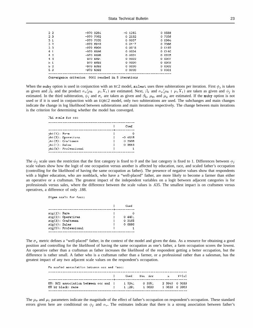
Stata Technical Bulletin 23
2.2 -970.9284 -0.1285 0.9588
2.3 -970.7092 0.2192 0.7038
3.1 -970.7035 0.0057 0.0964
3.2 -970.6918 0.0117 0.2366
3.3 -970.6900 0.0018 0.0192
4.1 -970.6896 0.0004 0.0140
4.2 -970.6895 0.0001 0.0023
4.3 -970.6894 0.0002 0.0007
5.1 -970.6893 0.0000 0.0003
5.2 -970.6893 0.0000 0.0002
5.3 -970.6893 0.0000 0.0001
----------------------------------------------------------------------
Convergence criterion .0001 reached in 5 iterations
When the muby option is used in conjunction with an RC2 model, mclest uses three subiterations per iteration. First �j is takenas given and �k and the product �v(�0 + �1X1) are estimated. Next, �k and �v(�0 + �1X1) are taken as given and �j isestimated. In the third subiteration, �j and �v are taken as given and �k, �0, and �1 are estimated. If the muby option is notused or if it is used in conjunction with an EQRC2 model, only two subiterations are used. The subchanges and main changesindicate the change in log likelihood between subiterations and main iterations respectively. The change between main iterationsis the criterion for determining whether the model has converged.
Phi scale for occ
-------------------------------------------------
| Coef.
-------------------------------------+-----------
phi(1): Farm | 0
phi(2): Operatives | -0.4818
phi(3): Craftsmen | -0.2938
phi(4): Sales | 0.3653
phi(5): Professional | 1
-------------------------------------------------
The �j scale uses the restriction that the first category is fixed to 0 and the last category is fixed to 1. Differences between �jscale values show how the logit of one occupation versus another is affected by education, race, and scaled father’s occupation(controlling for the likelihood of having the same occupation as father). The presence of negative values show that respondentswith a higher education, who are nonblack, who have a “well-placed” father, are more likely to become a farmer than eitheran operative or a craftsman. The greatest impact of the independent variables on a logit between adjacent categories is forprofessionals versus sales, where the difference between the scale values is .635. The smallest impact is on craftsmen versusoperatives, a difference of only .188.
Sigma scale for focc:
-------------------------------------------------
| Coef.
-------------------------------------+-----------
sig(1): Farm | 0
sig(2): Operatives | 0.4401
sig(3): Craftsmen | 0.3165
sig(4): Sales | 0.6886
sig(5): Professional | 1
-------------------------------------------------
The �v metric defines a “well-placed” father, in the context of the model and given the data. As a resource for obtaining a goodposition and controlling for the likelihood of having the same occupation as one’s father, a farm occupation scores the lowest.An operative rather than a craftsman as father increases the likelihood of the respondent getting a better occupation, but thedifference is rather small. A father who is a craftsman rather than a farmer, or a professional rather than a salesman, has thegreatest impact of any two adjacent scale values on the respondent’s occupation.
Mu scaled association between occ and focc:
-------------------------------------------------------------------------------
| Coef. Std. Err. z P>|z|
-------------------------------------+-----------------------------------------
MU: RC2 association between occ and | 1.0241 0.3551 2.8840 0.0039
MU by black: race | 1.1291 1.0633 1.0619 0.2883
-------------------------------------------------------------------------------
The �0 and �1 parameters indicate the magnitude of the effect of father’s occupation on respondent’s occupation. These standarderrors given here are conditional on �j and �v . The estimates indicate that there is a strong association between father’s

24 Stata Technical Bulletin STB-56
occupation and respondent’s occupation but that this is not significantly different for blacks and nonblacks. The impact ofhaving a father who is a professional rather than a salesman on the logit of becoming a professional rather than a salesman is(1� :689)1.024(1� :365) = :202 for nonblacks and (1� :689)(1.024 + 1.129)(1� :365) = :426 for blacks (noting that �1 islarge but also has a large standard error and is not significant).
Beta parameters:
-------------------------------------------------------------------------------
| Coef. Std. Err. z P>|z|
-------------------------------------+-----------------------------------------
SOR effect for educ: education in ye | 0.4406 0.0343 12.8461 0.0000
SOR effect for black: race | -1.4045 0.5878 -2.3896 0.0169
-------------------------------------------------------------------------------
These are the SOR effects of education and race. The impact of one year of education on the logit of becoming a professionalversus a salesman is :441(1� :365) = :280. The impact of being black rather than nonblack is �1.405(1� :365) = �:891.
Full parameter listing:
Conditional (fixed-effects) logistic regression Number of obs = 4190
LR chi2(13) = 756.04
Prob > chi2 = 0.0000
Log likelihood = -970.6893 Pseudo R2 = 0.2803
------------------------------------------------------------------------------
__didep | Coef. Std. Err. z P>|z| [95% Conf. Interval]
---------+--------------------------------------------------------------------
Iocc_2 | 6.528278 .5511616 11.845 0.000 5.448021 7.608535
Iocc_3 | 5.436115 .5270407 10.314 0.000 4.403134 6.469096
Iocc_4 | .8334484 .5414884 1.539 0.124 -.2278494 1.894746
Iocc_5 | -2.480348 .7093216 -3.497 0.000 -3.870593 -1.090103
Idiag_1 | 3.442951 .5782425 5.954 0.000 2.309617 4.576285
Idiag_2 | .5049115 .1881059 2.684 0.007 .1362307 .8735924
Idiag_3 | .4020211 .1897849 2.118 0.034 .0300496 .7739927
Idiag_4 | -.4116733 .3947225 -1.043 0.297 -1.185315 .3619686
Idiag_5 | -.5496774 .2975123 -1.848 0.065 -1.132791 .0334361
__beta1 | .4406277 .0343005 12.846 0.000 .3734001 .5078554
__beta2 | -1.404548 .5877656 -2.390 0.017 -2.556548 -.252549
__mu | 1.024126 .3551078 2.884 0.004 .3281276 1.720125
__muby1 | 1.129056 1.06328 1.062 0.288 -.9549348 3.213046
------------------------------------------------------------------------------
These are the estimates from the final subiteration. Standard errors are conditional, given �j and �v . The first four parametersare standard multinomial logistic intercepts. The Idiag * parameters measure the likelihood of the respondent having the sameoccupation as his father. Having a father who is a farmer has a tremendous impact on the logit for becoming a farmer versusany other occupation. The Idiag 4 and Idiag 5 parameters for sales and professional occupations are negative, reducing theimpact of the RC2 effect if father and son both have either of these occupations. The remaining parameters have been treatedabove.
Normalized Solution:
Normalized phi scale for occ:
-------------------------------------------------
| Coef.
-------------------------------------+-----------
phi(1): Farm | -0.1003
phi(2): Operatives | -0.5101
phi(3): Craftsmen | -0.3502
phi(4): Sales | 0.2104
phi(5): Professional | 0.7502
-------------------------------------------------
Normalized Sigma scale for focc:
-------------------------------------------------
| Coef.
-------------------------------------+-----------
sig(1): Farm | -0.6465
sig(2): Operatives | -0.0647
sig(3): Craftsmen | -0.2281
sig(4): Sales | 0.2638
sig(5): Professional | 0.6755
-------------------------------------------------

Stata Technical Bulletin 25
Unless the nonorm option is used, mclgen also produces a normalized solution. The scaling metrics now have a mean of zeroand a sum of squares of 1.
Iteration 0: log likelihood = -1218.2183
Iteration 1: log likelihood = -1000.3561
Iteration 2: log likelihood = -976.65487
Iteration 3: log likelihood = -971.5582
Iteration 4: log likelihood = -970.73319
Iteration 5: log likelihood = -970.6895
Iteration 6: log likelihood = -970.6893
Conditional (fixed-effects) logistic regression Number of obs = 4190
LR chi2(13) = 756.04
Prob > chi2 = 0.0000
Log likelihood = -970.6893 Pseudo R2 = 0.2803
------------------------------------------------------------------------------
__didep | Coef. Std. Err. z P>|z| [95% Conf. Interval]
---------+--------------------------------------------------------------------
Iocc_2 | 6.286966 .5487816 11.456 0.000 5.211373 7.362558
Iocc_3 | 5.288965 .5245917 10.082 0.000 4.260784 6.317145
Iocc_4 | 1.016421 .5376269 1.891 0.059 -.0373089 2.07015
Iocc_5 | -1.979513 .7071723 -2.799 0.005 -3.365545 -.5934809
Idiag_1 | 3.442951 .5782421 5.954 0.000 2.309617 4.576285
Idiag_2 | .5049115 .1881059 2.684 0.007 .1362307 .8735924
Idiag_3 | .4020211 .1897849 2.118 0.034 .0300496 .7739927
Idiag_4 | -.4116732 .3947225 -1.043 0.297 -1.185315 .3619686
Idiag_5 | -.5496775 .2975123 -1.848 0.065 -1.132791 .033436
__beta1 | .5180692 .0403289 12.846 0.000 .4390261 .5971123
__beta2 | -1.002211 .3355206 -2.987 0.003 -1.659819 -.3446024
__mu | .9108703 .3158372 2.884 0.004 .2918408 1.5299
__muby1 | 1.004196 .9456943 1.062 0.288 -.8493306 2.857723
------------------------------------------------------------------------------
These are the parameter estimates, given the normalized �j and �v scaling metrics. Which set of parameters is used is basicallya matter of personal preference.
Syntax for mclgen
mclgen depvar
The argument depvar, a categorical response factor with a maximum of 12 levels, must be specified for use in the MCL
model. Note that the mclgen program will modify the data and that the data should therefore be saved before running it. Besidestransforming the data into a person/choice file, mclgen adds didep and strata, the dichotomous dependent variable andstratifying variable used by clogit. In addition, it defines the global macros ncat containing the number of categories of theresponse variable and respfact, the name of the response factor.
Syntax for mclest
mclest varlist�weight
� �if exp
� �in range
� �, sor(varlist) soriter(#) sortol(#) rc2(varname)
eqrc2(varname) muby(varlist) nonorm debug�
fweights and iweights are allowed.
mclest is used to estimate a model after transforming the data to a “person/choice” file using mclgen. The varlist shouldcontain dummies based on the response factor specified in mclgen and interactions of these dummies with independent variables.This design matrix can be specified using xi or desmat (Hendrickx 1999).
mclest passes the weight, if, and in arguments to clogit unaltered. See the Stata documentation on clogit for furtherdetails.
Options
The following options are used to request the special nonlinear models Stereotyped Ordered Regression (SOR) and/or theRow and Columns model 2 (RC2).
sor(varlist) specifies a list of variables for which the SOR constraint should be used. Note that at least two variables should bespecified, unless either the rc2 or eqrc2 option is being used.
soriter(#) specifies the maximum number of iterations for estimating a SOR or RC2 model. The default value is 10.

26 Stata Technical Bulletin STB-56
sortol(#) specifies the convergence criterion for estimating a SOR or RC2 model. The default value is .0001.
rc2(varname) specifies a categorical independent variable for which the RC2 model is to be used. The eqrc2 option will beignored if the rc2 option is specified.
eqrc2(varname) specifies a categorical independent variable for which the EQRC2 model is to be used. The rc2 option maynot be used together with the eqrc2 option.
muby(varlist) specifies one or more variables that affect the association between the rc2 or eqrc2 variable and the dependentvariable. This option is ignored if not used in conjunction with the rc2 or eqrc2 option.
nonorm prevents the mclest program from estimating a normalized solution if a SOR and/or RC2 model has been requested.
debug prints intermediate results of clogit. This can be used to determine the source of error if something goes wrong.
Recovering data
mclgen and mclest create a number of variables for internal use when estimating models. To transform the person/choicefile back to its original form, specify
. keep if __didep==1
. drop __*
ReferencesAnderson, J. A. 1984. Regression and ordered categorical variables. Journal of the Royal Statistical Society, Series B 46: 1–30.
Breen, R. 1994. Individual level models for mobility tables and other cross-classifications. Sociological Methods & Research 33: 147–173.
DiPrete, T. A. 1990. Adding covariates to loglinear models for the study of social mobility. American Sociological Review 55: 757–773.
Goodman, L. A. 1979. Multiplicative models for the analysis of occupational mobility tables and other kinds of cross-classification tables. AmericanJournal of Sociology 84: 804–819.
Hendrickx, J. 1999. dm73: Using categorical variables in Stata. Stata Technical Bulletin 52: 2–8. Reprinted in Stata Technical Bulletin Reprints,vol. 9, pp. 51–59.
Logan, J. A. 1983. A multivariate model for mobility tables. American Journal of Sociology 89: 324–349.
sg143 Cronbach’s alpha one-sided confidence interval
Maria-Jose Bleda, Madrid, Spain, [email protected] Tobias, Universidad Miguel Hernandez, Alicante, Spain, [email protected]
Abstract: Cronbach’s alpha has been commonly used to assess the reliability for summative rating scales. However, Cronbach’salpha is a lower bound of reliability, thus a one-sided confidence interval can be calculated. The cialpha commandcomputes the Cronbach’s alpha one-sided confidence interval.
Keywords: Cronbach’s alpha, reliability, rating scales, confidence interval.
Introduction
Cronbach’s alpha (Cronbach 1951) assesses the reliability of a summative rating scale composed of the items specified.This can be easily computed in Stata using the alpha command. It is also demonstrated that Cronbach’s alpha is always a lowerbound of reliability (Guttman 1953). Thus, a one-sided confidence interval can be easily computed (Kristoff 1963, Feldt 1965).Although this result is well known and confidence intervals are commonly used in statistics, it is rarely applied by researchersevaluating instruments yielding a continuous measure (Bravo and Potvin 1991). In this way, Stata usually provides confidenceintervals with most parameter estimates, but a confidence interval for Cronbach’s alpha is not provided by the alpha command.In this insert we provide the command cialpha, which computes the Cronbach’s alpha one-sided confidence interval.
Method
Kristoff (1963) and Feldt (1965) independently derived a transformation of the sample Cronbach’s alpha coefficient, whichthey showed has an F distribution. From their sampling theory, a one-sided confidence interval can be shown to be given by
�X � 1��(1� b�X)Fa;n�1;(k�1)(n�1)
�= �L
This value enables one to determine whether the value achieved is significantly greater than some minimum value.

Stata Technical Bulletin 27
Syntax
cialpha�, level(#)
�cialpha can only be run after the alpha command, see [R] alpha.
Options
level(#) specifies the confidence level, in percent, for confidence intervals. The default is level(95) or as set by set level.
Example
To illustrate the cialpha command, we consider Stata’s automobile data. The scale derived from the arbitrarily chosenautomobile items appears rather good, since alpha gives a value of 0.8975.
. alpha price hdroom rep78 trunk weight length turn displ, std
Test scale = mean(standardized items)
Reversed item: rep78
Average interitem correlation: 0.5225
Number of items in the scale: 8
Scale Reliability Coefficient: 0.8975
Then, the 95% one-sided confidence interval for Cronbach’s alpha has lower limit 0.8651.
. cialpha
Cronbach's alpha one-sided confidence interval
------------------------------------------------------------------------------
Items | alpha [95% Conf.Interval]
---------+--------------------------------------------------------------------
Test | .89746938 >= .86513734
------------------------------------------------------------------------------
This means that there is a 95% chance that the Cronbach’s alpha will be higher than this value.
Saved results
cialpha saves in r()
r(alpha) scale reliability coefficient r(ci) one-sided confidence intervalr(k) number of items in the table r(level) specifies the confidence levelr(n) number of observations
ReferencesBravo, G. and L. Potvin. 1991. Estimating the reliability of continuous measures with Cronbach’s alpha or the intraclass correlation coefficient: toward
the integration of two traditions. Journal of Clinical Epidemiology 44: 381–390.
Cronbach, L. J. 1951. Coefficient alpha and the internal structure of a test. Psychometrika 16: 297–334.
Feldt L. S. 1965. The approximate sampling distribution of Kuder–Richardson reliability coefficient twenty. Psychometrika 30: 357–371.
Guttman L. 1953. Reliability formulas that do not assume experimental independence. Psychometrika 18: 225–239.
Kristoff W. 1963. The statistical theory of stepped-up reliability coefficients when a test has been divided into several equivalent parts. Psychometrika28: 221–238.
sg144 Marginal effects of the tobit model
Ronna Cong, Stata Corporation, [email protected]
Abstract: This article describes the dtobit command which provides a table of four forms of marginal effects for a tobitmodel. The marginal effects are computed for the latent dependent variable, the expected value of the dependent variableconditional on being uncensored, the unconditional expected value of the dependent variable, and the probability of beinguncensored. The article also includes a brief discussion of the McDonald and Moffitt decomposition. Several examples areused to illustrate how this command can be run and how to interpret the output.
Keywords: tobit model, marginal effects of the tobit model, McDonald and Moffitt decomposition.

28 Stata Technical Bulletin STB-56
Syntax
dtobit�, at(matname) censor brief nodiscrete level(#)
�dtobit is for use after estimation by tobit; see [R] tobit.
Description
dtobit provides a table of marginal effects evaluated at the means of the independent variables by default, or at theobserved censoring rate of the dependent variable if censor is specified, or at user specified points if at(matname) is specified.The marginal effects are computed for the latent dependent variable, the expected value of the dependent variable conditionalon being uncensored, the unconditional expected value of the dependent variable, and the probability of being uncensored. Fordummy variables, dtobit will report the discrete changes unless the nodiscrete option is specified.
Options
at(matname) specifies the points around which the marginal effects are to be estimated. The default is to estimate the effectsaround the means of the independent variables.
censor specifies that the marginal effects should be evaluated at the observed censoring rate of the dependent variable. Thisoption is not allowed with the two-tailed censoring case. at(matname) and censor cannot be specified at the same time.
brief will simplify the output. Standard deviations of the estimates and the confidence intervals will be excluded from the table.
nodiscrete treats dummy variables as continuous. If nodiscrete is not specified, the marginal effect of a dummy variable iscalculated as the discrete change in the expected value of the dependent variable as the dummy variable changes from 0 to1.
level(#) specifies the confidence level, in percent, for confidence intervals. The default is level(95) or as set by set level;see [U] 23.5 Specifying the width of confidence intervals.
Marginal effects of the tobit model
Let y = X� + � be the latent regression model. y represents continuous outcomes either observed or not observed. Ourmodel assumes that � � N(0; �2I).
Let a be the lower censored limit, and b be the upper censored limit. The tobit model can be expressed by the followingrelationship:
y�i=
(yi if a < yi < b
a if yi � a
b if yi � b
For the tobit model, there are four forms of marginal effects that are of great interest:
1. the � coefficients themselves are the changes in the mean of the latent dependent variable: � = @E(yi)=@xi
2. the changes in the unconditional expected value of the observed dependent variable: @E(y�i)=@xi
3. the changes in the conditional expected value of the dependent variable: @E(y�ij a < y�
i< b)=@xi
4. the changes in the probability of being uncensored: @P (a < y�i< b)=@xi
Example
We will demonstrate dtobit using an admittedly contrived example with the auto dataset. First, we run tobit. Assumethat our data is censored in the sense that we cannot observe a mileage rating below 17 mpg, that is, if the true mpg is 17 orless, all we know is that the mpg is less than or equal to 17.
. use auto, clear
. tobit mpg trunk weight, ll(17)
Tobit estimates Number of obs = 74
LR chi2(2) = 73.86
Prob > chi2 = 0.0000
Log likelihood = -163.74787 Pseudo R2 = 0.1840
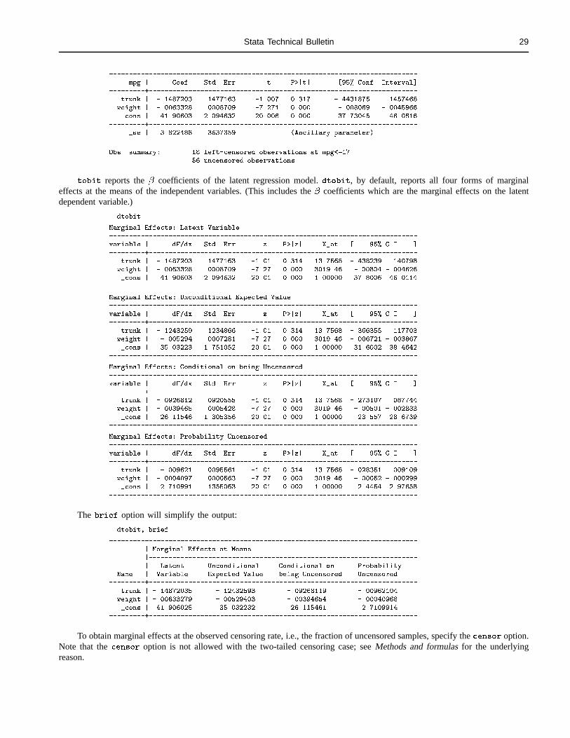
Stata Technical Bulletin 29
------------------------------------------------------------------------------
mpg | Coef. Std. Err. t P>|t| [95% Conf. Interval]
---------+--------------------------------------------------------------------
trunk | -.1487203 .1477163 -1.007 0.317 -.4431875 .1457468
weight | -.0063328 .0008709 -7.271 0.000 -.008069 -.0045966
_cons | 41.90603 2.094632 20.006 0.000 37.73045 46.0816
---------+--------------------------------------------------------------------
_se | 3.822488 .3637359 (Ancillary parameter)
------------------------------------------------------------------------------
Obs. summary: 18 left-censored observations at mpg<=17
56 uncensored observations
tobit reports the � coefficients of the latent regression model. dtobit, by default, reports all four forms of marginaleffects at the means of the independent variables. (This includes the � coefficients which are the marginal effects on the latentdependent variable.)
. dtobit
Marginal Effects: Latent Variable
------------------------------------------------------------------------------
variable | dF/dx Std. Err. z P>|z| X_at [ 95% C.I. ]
---------+--------------------------------------------------------------------
trunk | -.1487203 .1477163 -1.01 0.314 13.7568 -.438239 .140798
weight | -.0063328 .0008709 -7.27 0.000 3019.46 -.00804 -.004626
_cons | 41.90603 2.094632 20.01 0.000 1.00000 37.8006 46.0114
------------------------------------------------------------------------------
Marginal Effects: Unconditional Expected Value
------------------------------------------------------------------------------
variable | dF/dx Std. Err. z P>|z| X_at [ 95% C.I. ]
---------+--------------------------------------------------------------------
trunk | -.1243259 .1234866 -1.01 0.314 13.7568 -.366355 .117703
weight | -.005294 .0007281 -7.27 0.000 3019.46 -.006721 -.003867
_cons | 35.03223 1.751052 20.01 0.000 1.00000 31.6002 38.4642
------------------------------------------------------------------------------
Marginal Effects: Conditional on being Uncensored
------------------------------------------------------------------------------
variable | dF/dx Std. Err. z P>|z| X_at [ 95% C.I. ]
---------+--------------------------------------------------------------------
trunk | -.0926812 .0920555 -1.01 0.314 13.7568 -.273107 .087744
weight | -.0039465 .0005428 -7.27 0.000 3019.46 -.00501 -.002883
_cons | 26.11546 1.305356 20.01 0.000 1.00000 23.557 28.6739
------------------------------------------------------------------------------
Marginal Effects: Probability Uncensored
------------------------------------------------------------------------------
variable | dF/dx Std. Err. z P>|z| X_at [ 95% C.I. ]
---------+--------------------------------------------------------------------
trunk | -.009621 .0095561 -1.01 0.314 13.7568 -.028351 .009109
weight | -.0004097 .0000563 -7.27 0.000 3019.46 -.00052 -.000299
_cons | 2.710991 .1355063 20.01 0.000 1.00000 2.4454 2.97658
------------------------------------------------------------------------------
The brief option will simplify the output:
. dtobit, brief
------------------------------------------------------------------------------
| Marginal Effects at Means
|--------------------------------------------------------------------
| Latent Unconditional Conditional on Probability
Name | Variable Expected Value being Uncensored Uncensored
---------+--------------------------------------------------------------------
trunk | -.14872035 -.12432593 -.09268119 -.00962104
weight | -.00633279 -.00529403 -.00394654 -.00040968
_cons | 41.906025 35.032232 26.115461 2.7109914
---------+--------------------------------------------------------------------
To obtain marginal effects at the observed censoring rate, i.e., the fraction of uncensored samples, specify the censor option.Note that the censor option is not allowed with the two-tailed censoring case; see Methods and formulas for the underlyingreason.

30 Stata Technical Bulletin STB-56
. dtobit, censor brief
------------------------------------------------------------------------------
| Marginal Effects at Observed Censoring Rate
|--------------------------------------------------------------------
| Latent Unconditional Conditional on Probability
Name | Variable Expected Value being Uncensored Uncensored
---------+--------------------------------------------------------------------
trunk | -.14872035 -.11254513 -.08042806 -.01218351
weight | -.00633279 -.00479238 -.00342478 -.0005188
_cons | 41.906025 31.712668 22.662807 3.4330384
---------+--------------------------------------------------------------------
To obtain marginal effects at particular points of the independent variables, specify the at() option. For example, supposewe would like to obtain marginal effects at trunk = 12 and weight = 2500:
. mat M=(12, 2500, 1)
. dtobit, at(M) brief
------------------------------------------------------------------------------
| Marginal Effects at e(at)
|--------------------------------------------------------------------
| Latent Unconditional Conditional on Probability
Name | Variable Expected Value being Uncensored Uncensored
---------+--------------------------------------------------------------------
trunk | -.14872035 -.14451729 -.12916254 -.00251919
weight | -.00633279 -.00615381 -.00549998 -.00010727
_cons | 41.906025 40.721699 36.395078 .70985111
---------+--------------------------------------------------------------------
Example
Dummy variables are treated differently by dtobit. With dummy variables (or indicators), we are typically interested inthe net effect on a form of the dependent variable when the indicator changes from 0 to 1; the marginal effect of a discretechange in the indicator variable. This is what dtobit calculates by default. If the instantaneous rate of change for a one-unitchange in the indicator is desired, that is to say, if we want to treat the dummy variable like a continuous variable, we canspecify the nodiscrete option.
In the auto dataset, foreign is a dummy variable. Assume that we are interested in its effect on mileage rating. Whatwould be the difference in mileage between a foreign car (foreign = 1) and a domestic car (foreign = 0) given the sameweight and trunk space?
. tobit mpg trunk weight for , ll(17)
Tobit estimates Number of obs = 74
LR chi2(3) = 77.09
Prob > chi2 = 0.0000
Log likelihood = -162.13558 Pseudo R2 = 0.1921
------------------------------------------------------------------------------
mpg | Coef. Std. Err. t P>|t| [95% Conf. Interval]
---------+--------------------------------------------------------------------
trunk | -.1288913 .1458352 -0.884 0.380 -.4196784 .1618959
weight | -.0072948 .0010278 -7.097 0.000 -.0093442 -.0052454
foreign | -2.249467 1.2558 -1.791 0.078 -4.753461 .2545274
_cons | 45.15628 2.794429 16.159 0.000 39.58434 50.72821
---------+--------------------------------------------------------------------
_se | 3.763147 .3574121 (Ancillary parameter)
------------------------------------------------------------------------------
Obs. summary: 18 left-censored observations at mpg<=17
56 uncensored observations
. dtobit, brief
------------------------------------------------------------------------------
| Marginal Effects at Means
|--------------------------------------------------------------------
| Latent Unconditional Conditional on Probability
Name | Variable Expected Value being Uncensored Uncensored
---------+--------------------------------------------------------------------
trunk | -.12889128 -.10781396 -.08040115 -.00845294
weight | -.00729477 -.00610187 -.00455041 -.00047841
foreign*| -2.2494667 -2.171794 -1.8423142 -.16425745
_cons | 45.156276 37.771965 28.168056 2.9614379
---------+--------------------------------------------------------------------
(*) dF/dx is for discrete change of dummy variable from 0 to 1

Stata Technical Bulletin 31
The results above indicate that we would expect a higher mileage rating in domestic cars than foreign cars given thatweight and trunk space are taken at their means. A foreign car with mean weight and trunk space would have a 2.17 decreasein unconditional expected mileage and a 1.84 decrease in conditional expected mileage. Moreover, a typical domestic car has a.16 higher probability of being uncensored than that of a foreign car.
McDonald and Moffitt decomposition
A simple case of the tobit model, and probably the most useful one, is
yi = X� + �
y�i=
�yi if yi > 0
0 if yi � 0
A very interesting feature of this simplified tobit model was discovered by McDonald and Moffitt (1980). Consider theexpectation of y�:
E(y�) = P (y� > 0)E(y�jy� > 0)
The effect of a change in the jth continuous variable of X on E(y�) can be expressed as
@E(y�)=@xj = P (y� > 0)@E(y�jy� > 0)=@xj + E(y�jy� > 0)@P (y� > 0)=@xj
Thus the total change in the unconditional expected value of y� can be decomposed into two very intuitive parts:
1. the change in the expected value of y� of those above zero, weighted by the probability of being above zero;
2. the change in the probability of being above zero, weighted by the conditional expected value of y�.
Example
To illustrate the decomposition, we need to modify our auto dataset.
. replace mpg = mpg - 17
. tobit mpg trunk weight, ll(0)
Tobit estimates Number of obs = 74
LR chi2(2) = 73.86
Prob > chi2 = 0.0000
Log likelihood = -163.74787 Pseudo R2 = 0.1840
------------------------------------------------------------------------------
mpg | Coef. Std. Err. t P>|t| [95% Conf. Interval]
---------+--------------------------------------------------------------------
trunk | -.1487203 .1477163 -1.007 0.317 -.4431875 .1457468
weight | -.0063328 .0008709 -7.271 0.000 -.008069 -.0045966
_cons | 24.90603 2.094632 11.890 0.000 20.73045 29.0816
---------+--------------------------------------------------------------------
_se | 3.822488 .3637359 (Ancillary parameter)
------------------------------------------------------------------------------
Obs. summary: 18 left-censored observations at mpg<=0
56 uncensored observations
. dtobit, brief
------------------------------------------------------------------------------
| Marginal Effects at Means
|--------------------------------------------------------------------
| Latent Unconditional Conditional on Probability
Name | Variable Expected Value being Uncensored Uncensored
---------+--------------------------------------------------------------------
trunk | -.14872035 -.12432593 -.09268119 -.00962104
weight | -.00633279 -.00529403 -.00394654 -.00040968
_cons | 24.906025 20.820721 15.521213 1.6112246
---------+--------------------------------------------------------------------
In order to numerically show that the decomposition holds, we will use predict, e(0,.) to get the conditional expectedvalue at the means of trunk and weight, and predict, p(0,.) to get the probability of being above zero. We will use an addedobservation at the end of the data to create a record of mean values, the point where we have evaluated the marginal effects.

32 Stata Technical Bulletin STB-56
. mat list e(at)
e(at)[1,3]
trunk weight _cons
_cons 13.756757 3019.4595 1
. set obs 75
obs was 74, now 75
. replace trunk = 13.756757 in 75
trunk was int now float
(1 real change made)
. replace weight = 3019.4595 in 75
weight was int now float
(1 real change made)
. predict e, e(0,.)
. predict p, p(0,.)
. list e in 75 /* the conditional expected value */
e
75. 4.869236
. list p in 75 /* the probability for above zero */
p
75. .8359712
Now let’s see if the decomposition holds:
. display -.09268119*.8359712 + (-.00962104)*4.869236
-.12432592
As we expected, the decomposition recovers the change in the unconditional expected value of mileage.
Technical notes
The application of the decomposition was well illustrated in McDonald and Moffitt’s paper. There is no doubt that thedecomposition is useful. However, the decomposition will only hold when the limit is zero, and when the variable is continuous.Let’s consider both of these cases.
Decomposition with dummy variables
For dummy variables, the decomposition no longer holds. However, we can show a similar decomposition. Consider themarginal effects of dummy variable Xj :
E1(y�)� E0(y
�) = P1(y� > 0)E1(y
�jy� > 0)� P0(y� > 0)E0(y
�jy� > 0)
= P1(y� > 0) [E1(y
�jy� > 0)� E0(y�jy� > 0)] + E0(y
�jy� > 0) [P1(y� > 0)� P0(y
� > 0)]
= P0(y� > 0) [E1(y
�jy� > 0)� E0(y�jy� > 0)] + E1(y
�jy� > 0) [P1(y� > 0)� P0(y
� > 0)]
whereP1 is the probability evaluated at xj = 1
P0 is the probability evaluated at xj = 0
E1 is the expected value evaluated at xj = 1
E0 is the expected value evaluated at xj = 0
Thus the total change in the unconditional expected value of y� can also be decomposed into two parts:
1. the change in the expected value of y� of those above zero, weighted by the probability of being above zero given xj = 1
(or xj = 0);
2. the change in the probability of being above zero, weighted by the conditional expected value of y� given xj = 0 (orxj = 1).
Decomposition with specified censoring points
For the more general tobit model where the lower limit is a and the upper limit is b, the expected value of y� is
E(y�) = P (y� > 0)E(y�jy� > 0) + aP (y� < a) + bP (y� > b)

Stata Technical Bulletin 33
Thus, besides the change in conditional expected y� and the change in the probability of being uncensored, we need alsoconsider the change in the probability of being below a and the change in the probability of being above b.
Saved results
In addition to the standard saved results from tobit, dtobit saves in e():
Scalarse(rate) uncensored rate
Macrose(dummy) 0 indicates continuous, 1 indicates dummy
Matricese(b) marginal effects for the latent variable e(se c) standard deviations of e(dfdx c)
e(se b) standard deviations of e(b) e(dfdx p) marginal effects for the uncensored probabilitye(dfdx u) marginal effects for the unconditional expected value e(se p) standard deviations of e(dfdx p)
e(se u) standard deviations of e(dfdx u) e(at) points at which marginal effects were computede(dfdx c) marginal effects for the conditional expected value
Methods and formulas
dtobit is implemented as an ado-file.
Let y = X�+ � be the model. y represents continuous outcomes either observed or not observed. Our model assumes that� � N(0; �2I).
Let a be the lower limit, and b be the upper limit.
y�i=
(yi if a < yi < b
a if yi � a
b if yi � b
For the simple case where a = 0 and b = +1, let z = X�=�, f(z) be the standard normal density, and F (z) be the cumulativenormal distribution function, then
E(y�) = X�F (z) + �f(z)
E(y�jy� > 0) = X� + �f(z)=F (z)
P (y� > 0) = F (z)
The marginal effects for continuous variable xj are
@E(y�)=@xj = F (z)�j (unconditional expected value)
@E(y�jy� > 0)=@xj = �j
h1� zf(z)=F (z)� f(z)
2=F (z)
2i
(conditional expected value)
@P (y� > 0)=@xj = f(z)�j=� (probability uncensored)
For the more general case, let �a = (a�X�) =�, �b = (b�X�) =�, and fj = f(j) Fj = F (j). Then
E(y�) = aFa + b(1� Fb) + (Fb � Fa)X� + �(fa � fb)
E(y�ja < y� < b) = X� + �(fa � fb)=(Fb � Fa)
P (a < y� < b) = Fb � Fa
The marginal effects for continuous variable xj are
@E(y�)=@xj = (Fb � Fa)�j (unconditional expected value)
@E(y�ja < y� < b)=@xj = �j
�1� �afa��bfb
Fa�Fb��fa�fb
Fa�Fb
�2�(conditional expected value)
@P (a < y� < b)=@xj = �j(fa � fb)=� (probability censored)

34 Stata Technical Bulletin STB-56
dtobit by default, calculates marginal effects at the means of the independent variables; it also allows the user to specifypoints where marginal effects are to be evaluated. A special feature of dtobit is that the user can ask dtobit to calculatemarginal effects at the uncensoring rate. The uncensoring rate is defined as the proportion of uncensored observations of thewhole dataset. If censoring is one tailed, the value of X� can be recovered from the uncensoring rate (for example, if the lowerlimit is a, then X� = � � invnorm(uncensoring rate) + a), and is used for further calculation. However, when censoring is twotailed, the value of X� cannot be recovered; thus, the censor option is not allowed with these cases.
For dummy variables, the marginal effects are calculated as the discrete change of the expected values (probability ofuncensoring) as dummy variables change from 0 to 1.
ReferenceMcDonald, J. F. and R. A. Moffitt. 1980. The uses of tobit analysis. The Review of Economics and Statistics 62: 318–387.
sg145 Scalar measures of fit for regression models
J. Scott Long, Indiana University, [email protected] Freese, University of Wisconsin-Madison, [email protected]
Abstract: fitstat is a post-estimation command that computes a variety of scalar measures of fit for assessing regressionmodels for categorical, limited, and count dependent variables. It also computes the AIC and BIC measures which can beused for selecting among non-nested models. By using the save and dif options, it is simple to compare measures of fitacross models.
Keywords: scalar measures of fit, AIC, BIC, pseudo-R2s, regression models.
Overview
Many scalar measures have been developed to summarize the overall goodness of fit for regression models of continuous,count, or categorical dependent variables. The post-estimation command fitstat calculates a large number of fit statistics forthe estimation commands clogit, cnreg, cloglog, gologit, intreg, logistic, logit, mlogit, nbreg, ologit, oprobit,omodel, poisson, probit, regress, zinb, and zip. With its saving() and using() options, the command also allows thecomparison of fit measures across two models. While fitstat duplicates some measures computed by other commands (e.g.,the pseudo-R2 in standard Stata output of lfit), fitstat adds many more measures and makes it convenient to comparemeasures across models. Details on the measures that are discussed below can be found in Long (1997) which cites the originalsources for each measure and provides further details on their derivation.
Before proceeding, a word of caution regarding the use of these measures. A scalar measure of fit can be useful in comparingcompeting models and ultimately in selecting a final model. Within a substantive area of research, measures of fit can provide arough index of whether a model is adequate. However, there is no convincing evidence that selecting a model that maximizes thevalue of a given measure results in a model that is optimal in any sense other than the model having a larger (or smaller) valueof that measure. While measures of fit provide some information, it is only partial information that must be assessed within thecontext of the theory motivating the analysis, past research, and the estimated parameters of the model being considered.
Syntax
fitstat�, saving(name) save using(name) dif bic force
�While many measures of fit are based on values returned by the estimation command, for some measures it is necessary tocompute additional statistics from the estimation sample. While fitstat does not include if and in options, analysis is basedon the sample defined by e(sample) from the last model estimated. Accordingly, fitstat is appropriate for models estimatedusing if and in restrictions in the original model. fitstat can also be used when models are estimated with weighted data.Here there are two limitations. First, some measures cannot be computed with some types of weights. Second, with pweights
we use values of the “pseudo-likelihoods” to compute our measures of fit. Given the heuristic nature of the various measures offit, we see no reason why the resulting measures would be appropriate. Also, fitstat ends with an error if the last estimationcommand does not return a value for the log-likelihood equation with only an intercept (that is, if e(ll 0) returns a missingvalue). This will occur, for example, if the noconstant option is used with the estimation command.
Options
saving(name) saves the computed measures in a matrix for subsequent comparisons. name cannot be longer than 4 characters.
save is equivalent to saving(0).
using(name) compares the fit measures for the current model with those of the model saved as name. name cannot be longerthan 4 characters.

Stata Technical Bulletin 35
dif is equivalent to using(0).
bic presents only BIC and other information measures. In comparing two models, fitstat reports the guidelines in Raftery(1996) for assessing the strength of one model over another.
force allows comparison of two models even when the number of observations or the estimation method varies between thetwo models.
Models and measures
Details on the measures of fit are given below. Here we only summarize which measures are computed for which models.Y indicates a measure is computed; N indicates the measure is not computed.
gologit
nbreg
logistic cnreg poisson
logit ologit clogit intreg zinb
regress probit cloglog oprobit mlogit tobit zip
Log-likelihood Y Y Y1 Y Y Y Y2
Deviance & LR chi-square Y Y Y Y Y Y Y
AIC, AIC�n, BIC, BIC0
Y Y Y Y Y Y YR2 & Adjusted R
2 Y N N N N N NEfron’s R
2 N Y Y N N N NMcFadden’s, ML, C&U’s R
2 N Y Y Y Y Y YCount & Adjusted Count R2 N Y Y Y Y3 N NVar(e), Var(y�) and M&Z’s R
2 N Y N Y N Y N
1. For cloglog the log likelihood for the intercept-only model does not correspond to the first step in the iterations.
2. For zip and zinb, the log likelihood for the intercepts-only model is calculated by estimating zipjzinb lhs-variable, inf( cons).
3. The adjusted count R2 is not defined for clogit.
Example
To compute fit statistics for a single model:
. use mroz, clear
(PSID 1976 from T. Mroz)
. * compute fit statistics for a single model
. logit lfp k5 k618 age wc hc lwg inc
Iteration 0: log likelihood = -514.8732
Iteration 1: log likelihood = -454.32339
Iteration 2: log likelihood = -452.64187
Iteration 3: log likelihood = -452.63296
Iteration 4: log likelihood = -452.63296
Logit estimates Number of obs = 753
LR chi2(7) = 124.48
Prob > chi2 = 0.0000
Log likelihood = -452.63296 Pseudo R2 = 0.1209
------------------------------------------------------------------------------
lfp | Coef. Std. Err. z P>|z| [95% Conf. Interval]
---------+--------------------------------------------------------------------
k5 | -1.462913 .1970006 -7.426 0.000 -1.849027 -1.076799
k618 | -.0645707 .0680008 -0.950 0.342 -.1978499 .0687085
age | -.0628706 .0127831 -4.918 0.000 -.0879249 -.0378162
wc | .8072738 .2299799 3.510 0.000 .3565215 1.258026
hc | .1117336 .2060397 0.542 0.588 -.2920969 .515564
lwg | .6046931 .1508176 4.009 0.000 .3090961 .9002901
inc | -.0344464 .0082084 -4.196 0.000 -.0505346 -.0183583
_cons | 3.18214 .6443751 4.938 0.000 1.919188 4.445092
------------------------------------------------------------------------------

36 Stata Technical Bulletin STB-56
. fitstat
Measures of Fit for logit of lfp
Log-Lik Intercept Only: -514.873 Log-Lik Full Model: -452.633
D(745): 905.266 LR(7): 124.480
Prob > LR: 0.000
McFadden's R2: 0.121 McFadden's Adj R2: 0.105
Maximum Likelihood R2: 0.152 Cragg & Uhler's R2: 0.204
McKelvey and Zavoina's R2: 0.217 Efron's R2: 0.155
Variance of y*: 4.203 Variance of error: 3.290
Count R2: 0.693 Adj Count R2: 0.289
AIC: 1.223 AIC*n: 921.266
BIC: -4029.663 BIC': -78.112
To compute and save fit measures:
. logit lfp k5 k618 age wc hc lwg inc
(output same as above ). fitstat, saving(mod1)
(output same as above )(Indices saved in matrix fs_mod1)
To compare the saved model to the current model:
. logit lfp k5 age age2 wc inc
(output omitted ). fitstat, using(mod1)
Measures of Fit for logit of lfp
Current Saved Difference
Model: logit logit
N: 753 753 0
Log-Lik Intercept Only: -514.873 -514.873 0.000
Log-Lik Full Model: -461.653 -452.633 -9.020
D: 923.306(747) 905.266(745) 18.040(2)
LR: 106.441(5) 124.480(7) -18.040(-2)
Prob > LR: 0.000 0.000 0.000
McFadden's R2: 0.103 0.121 -0.018
McFadden's Adj R2: 0.092 0.105 -0.014
Maximum Likelihood R2: 0.132 0.152 -0.021
Cragg & Uhler's R2: 0.177 0.204 -0.028
McKelvey and Zavoina's R2: 0.182 0.217 -0.035
Efron's R2: 0.135 0.155 -0.020
Variance of y*: 4.023 4.203 -0.180
Variance of error: 3.290 3.290 0.000
Count R2: 0.677 0.693 -0.016
Adj Count R2: 0.252 0.289 -0.037
AIC: 1.242 1.223 0.019
AIC*n: 935.306 921.266 14.040
BIC: -4024.871 -4029.663 4.791
BIC': -73.321 -78.112 4.791
Difference of 4.791 in BIC' provides positive support for saved model.
Saved results
fitstat saves in r() whichever of the following are computed for a particular model:
Scalarsr(aic) AIC r(n rhs) number of right hand side variablesr(aic n) AIC�n r(r2) R
2 for linear regression modelr(bic) BIC r(r2 adj) adjusted R
2 for linear regression modelr(bic p) BIC0 r(r2 ct) count R2
r(dev) deviance r(r2 ctadj) adjusted count R2
r(dev df) degrees of freedom for deviance r(r2 cu) Cragg & Uhler’s R2
r(ll) log-likelihood for full model r(r2 ef) Efron’s R2
r(ll 0) log-likelihood for model with only intercept r(r2 mz) McKelvey and Zavoina’s R2
r(lrx2) likelihood ratio chi-square r(r2 mf) McFadden’s R2
r(lrx2 df) degrees of freedom for likelihood ratio chi-square r(r2 mfadj) McFadden’s adjusted R2
r(lrx2 p) probability level of chi-square test r(r2 ml) maximum likelihood R2
r(N) number of observations r(v error) variance of error termr(n parm) number of parameters r(v ystar) variance of y�

Stata Technical Bulletin 37
When the saving(name) option is specified, computed measures are also saved in matrix fs name. The column namesof the matrix correspond to the names of the measures listed above. The row name is the command used to estimate the savedmodel. Values of �9999 in the matrix indicate that a measure is not appropriate for the given model. The row name is the nameof the estimation procedure.
Extending fitstat to other models and measures
fitstat can be extended to other models and measures of fit. When doing this, there are several things to keep in mind.First, the program depends on values returned by eclass estimation commands (for example, e(sample)). Programs such asocratio which do not use eclass returns cannot be incorporated into fitstat without major changes to the structure of theprogram. Second, not all measures of fit are appropriate for all models. The programmer must be careful to ensure that fitstatdoes not automatically compute inappropriate fit statistics. Third, the way in which values such as the number of parametersand the number of right-hand-side variables are computed differs across models. Consequently, additional code may be neededfor these computations.
Methods and formulas
In this section we provide brief descriptions of each measure computed by fitstat. Full details along with citations tooriginal sources are found in Long (1997). The measures are listed in the same order as the output illustrated above.
Log-likelihood based measures
Stata begins maximum likelihood iterations by computing the log likelihood of the model with all parameters except theintercept(s) constrained to zero, referred to as L(MIntercept) below. The log likelihood upon convergence, referred to as MFullbelow, is also listed. In Stata this information is usually presented as the first step of the iterations and in the header for theestimation results. Note that in cloglog, the value at iteration 0 is not the log likelihood with only the intercept. For zip
and zinb, the intercept-only model can be defined in different ways. These commands return as e(ll 0) the value of the loglikelihood with the binary portion of the model unrestricted while only the intercept is free for the Poisson or negative binomialportion of the model. Alternatively, fitstat returns the value of the log likelihood from the model with only an intercept inboth the binary and count portion of the model.
Chi-square test of all coefficients
A likelihood-ratio test of the hypothesis that all coefficients except the intercept(s) can be computed by comparing the loglikelihoods.
LR = 2 lnL(MFull)� 2 lnL(MIntercept)
This statistic is sometimes designated as G2. LR is reported by Stata as: LR chi2(7) = 124.48 where the degrees of freedom,(7), are the number of constrained parameters. fitstat reports this statistic as: LR(7): 124.48. For zip and zinb, LR teststhat the coefficients in the count portion (not the binary portion) of the model are zero.
Deviance
The deviance compares a given model to a model that has one parameter for each observation and can reproduce perfectlythe observed data. The deviance is defined as D = �2 lnL(MFull), where the degrees of freedom equals N minus the numberof parameters. Note that D does not have a chi-square distribution.
Coefficient of determination in the LRM
For regress, fitstat reports the standard coefficient of determination which can be defined variously as
R2 = 1�
PN
i=1 (yi � byi)2PN
i=1 (yi � y)2=
cVar(by)cVar(by) + cVar(b�) = 1�
�L(MIntercept)
L(MFull)
�2=NThe adjusted R2 is defined as
�R2 =
�R2 �
K
N � 1
��N � 1
N �K � 1
�where K is the number of independent variables.
Pseudo R-squared
While each of the definitions of R2 above give the same numeric value in the LRM, they give different answers and thusprovide different measures of fit when applied to the other models evaluated by fitstat.

38 Stata Technical Bulletin STB-56
McFadden’s R-squared
The McFadden R2, also known as the “likelihood ratio index,” compares a model with just the intercept to a model withall parameters. It is defined as
R2McF = 1�
ln bL (MFull)
ln bL �MIntercept�
If model MFull = MIntercept, R2McF equals 0, but R2
McF can never exactly equal one. This measure, which is computed by Stataas Pseudo R2 = 0.1209, is listed in fitstat as: McFadden's R2: 0.121 Since R2
McF always increases as new variables areadded, an adjusted version is also available
�R2McF = 1�
ln bL (MFull)�K�
ln bL �MIntercept�
where K� is the number of parameters (not independent variables).
Maximum likelihood R-squared
Another analogy to R2 in the LRM was suggested by Maddala.
R2ML = 1�
"L�MIntercept
�L (MFull)
#2=N= 1� exp(�G2=N)
Cragg & Uhler’s R-squared
Since R2ML only reaches a maximum of 1� L
�MIntercept
�2=N, Cragg and Uhler suggested a normed measure.
R2C&U =
R2ML
maxR2ML
=1�
�L�MIntercept
�=L (MFull)
�2=N1� L
�MIntercept
�2=NEfron’s R-squared
For binary outcomes, Efron’s pseudo-R2 defines by = b� = cPr (y = 1jx) and equals
R2Efron = 1�
PN
i=1 (yi � b�i)2PN
i=1 (yi � �y)2
McKelvey and Zavoina’s R-squared
Some models can be defined in terms of a latent variable y�. This includes the models for binary or ordinal outcomes;logit, probit, ologit and oprobit, as well as some models with censoring: tobit, cnreg, and intreg. Each model isdefined in terms of a regression on a latent variable y�:
y� = x� + �
Using cVar� by�� = b�0cVar (x) b�, McKelvey and Zavoina proposed
R2M&Z =
cVar� by��cVar (y�)
=cVar� by��cVar
� by��+ Var (�)
In models for categorical outcomes, Var(�) is assumed to identify the model; in models with censoring, it can be estimated.

Stata Technical Bulletin 39
Count and adjusted count R2
Observed and predicted values can be used in models with categorical outcomes to compute what is known as the countR2. Consider the binary case where the observed y is 0 or 1 and �i = cPr(y = 1jxi). Define the expected outcome by as
byi = �0 if b�i � 0:5
1 if b�i > 0:5
This allows us to construct a table of observed and predicted values, such as produced by the Stata command lstat:
-------- True --------
Classified | D ~D Total
-----------+--------------------------+-----------
+ | 342 145 | 487
- | 86 180 | 266
-----------+--------------------------+-----------
Total | 428 325 | 753
A seemingly appealing measure is the proportion of correct predictions, referred to as the count R2:
R2Count =
1
N
Xj
njj
where the njj’s are the number of correct predictions for outcome j. The count R2 can give the faulty impression that the modelis predicting very well. In a binary model without knowledge about the independent variables, it is possible to correctly predictat least 50 percent of the cases by choosing the outcome category with the largest percentage of observed cases. To adjust forthe largest row marginal, we have
R2AdjCount =
Pjnjj �maxr(nr+)
N �maxr(nr+)
where nr+ is the marginal for row r. The adjusted count R2 is the proportion of correct guesses beyond the number that wouldbe correctly guessed by choosing the largest marginal.
Information measures
This class of measures can be used to compare models across different samples or to compare nonnested models.
AIC
Akaike’s information criteria is defined as
AIC =�2 ln bL (Mk) + 2P
N
where bL (Mk) is the likelihood of the model and P is the number of parameters in the model (for example, K +1 in the binaryregression model where K is the number of regressors). All else being equal, the model with the smaller AIC is considered thebetter fitting model. Some authors define AIC as being N times the value we report. We report this quantity as AIC*n.
BIC and BIC0
The Bayesian information criterion has been proposed by Raftery (1996 and the literature cited therein) as a measure ofoverall fit and a means to compare nested and nonnested models. Consider the model Mk with deviance D (Mk). BIC is definedas:
BICk = D (Mk)� dfk lnN
where dfk is the degrees of freedom associated with the deviance. The more negative the BICk is, the better the fit. A secondversion of BIC is based on the LR chi-square with df 0
kequal to the number of regressors (not parameters) in the model. Then
BIC0k= �G2 (Mk) + df 0
klnN
The more negative the BIC0k
, the better the fit. The difference in the BICs from two models indicates which model is more likelyto have generated the observed data. Since BIC1 � BIC2 = BIC01 � BIC02, the choice of which BIC measure to use is a matter ofconvenience. If BIC1 � BIC2 < 0, then the first model is preferred. If BIC1 � BIC2 > 0, the second model is preferred. Raftery

40 Stata Technical Bulletin STB-56
suggested guidelines for the strength of evidence favoring M2 against M1 based on a difference in BIC or BIC0 as given in thetable below.
AbsoluteDifference Evidence
0–2 Weak2–6 Positive6–10 Strong> 10 Very strong
Acknowledgments
We thank David M. Drukker, Senior Statistician at Stata Corporation for his helpful suggestions.
ReferencesLong, J. S. 1997. Regression Models for Categorical and Limited Dependent Variables. Thousand Oaks, CA: Sage.
Raftery, A. E. 1996. Bayesian model selection in social research. In Sociological Methodology, ed. P. V. Marsden, 111–163. Oxford: Basil Blackwell.
sg146 Parameter estimation for the generalized extreme value distribution
Manuel G. Scotto, University of Lisbon, Portugal, [email protected] Tobias, Universidad Miguel Hernandez, Alicante, Spain, [email protected]
Abstract: In the analysis of extreme value data, such as wind speeds, air pollution levels, and river heights the generalized extremevalue distribution (GEVD) plays a basic role. We present a program to fit the GEVD using the method of probability-weightedmoments and the hybrid estimator proposed by Dupuis and Tsao.
Keywords: generalized extreme value distribution, extreme values, estimation, parameter, environmental statistics.
Introduction
In Scotto (2000) we considered the Gumbel distribution and its applications to environmental statistics. In this paper weturn our attention to the generalized extreme value distribution (GEVD).
Suppose we are interested in making inferences about extremal values of some random variables, for which we have adataset available, in such a way that it is reasonable to identify it with X1; : : : ; Xn, an independent, identically distributedsample with underlying model F , and denote by Mr the sample maximum. According to classical extreme value theory, thedistribution of linear functions of Mr can be approximated by taking limits as n ! 1 and approximating for large but finiten, by the GEVD
Gk;�;�(x) = exp
(�
�1�
k(x� �)
�
�1=k)where x is bounded by � + �=k from above if k > 0 and from below if k < 0. As usual, the case k = 0 corresponds to theGumbel distribution
G0;�;� = exp
�� exp
��x� �
�
��The parameter k is a shape parameter which determines the weight of the tail of G, while � and � are location and scaleparameters, respectively. The GEVD was introduced by Jenkinson (1955), and it has been successfully applied in modeling annualmaximum river heights, sea levels, and air pollutants.
Our main concern here is to obtain point estimates for the parameters k, �, and �. Commonly, the method of probability-weighted moments (PWM) (Greenwood et al. 1975) has been used for this purpose. However, as is known, this method frequentlyleads to nonfeasible estimates in the sense that the supports inferred from the estimates fail to contain all observations. Dupuisand Tsao (1998) proposed the hybrid estimator which is derived by incorporating an auxiliary constraint on feasibility into theestimates from PWM to produce feasible estimates. Both methods have been implemented in the gevd command described below.

Stata Technical Bulletin 41
Method of probability-weighted moments
The method of probability-weighted moments consists of equating model moments based on Gk;�;� to the correspondingempirical moments based on the data. The PWM method was developed by Greenwood et al. (1975). An overview of this methodis as follows. The probability-weighted moments of a random variable X with distribution function F are defined as
Mp;r;s = E [Xp fF (X)grf1� F (X)g
s]
where p, r and s are real numbers. To obtain PWM estimates for k, �, and �, it is convenient to fix p = 1 and s = 0 in theabove expression for Mp;r;s and use the quantities
�s = E [X fF (X)gs] =
� +�
k
�1�
�(1 + k)
(r + 1)k
�r + 1
which exist provided that k > �1. From this expression we obtain
�0 = � +�
�f1� �(1 + k)g (1)
2�1 � �0 =�
��(1 + k)(1� 2�k) (2)
3�2 � �1
2�1 � �2=
1� 3�k
1� 2�k(3)
The method consists in matching �0, �1, and �2 with appropriate sample equivalents b0, b1, and b2 in order to obtain thePWM estimators bk, b�, and b�. In general, bi may be taken as
bi = n�1
nXj=1
wi
jXj:n
where X1:n � X2:n � : : : � Xn:n are the ordered sample. The weights wj are defined as
wj =(j � 1)(j � 2) � � � (j � i)
(n� 1)(n� 2) � � � (n� i)
Clearly, equation (3) only depends on bk. The exact solution requires iterative methods, but since the function is almost linearover the range of interest (�0:5 < k < 0:5), which is usually encountered in practice, the following approximate low-orderpolynomial estimator (Hosking et al. 1985) is used
bk = 7:859c+ 2:955c2; c =2b1 � b0
3b2 � b0�
ln 2
ln 3(4)
The error due to using (4) insted of (3) is less than 0.0009 throughout the range (Hosking et al. 1985). Given bk, the scale andlocation parameters can be estimated successively from (1) and (2) as
b� =(2b1 � b0)bk
�(1 + bk)(1� 2�bk) b� = b0 +b�bkn�(1 + bk)� 1
oThe parameter estimate of the bound is thus b�+ b�=bk. The PWM estimates are not feasible when the following auxiliary constraintsare violated
Xn:n � b� + b�bk > 0
X1:n � b� + b�bk < 0
(5)
(Dupuis and Tsao 1998). For further details of the method see Hosking et al. (1985). See also Dupuis (1996) for an exhaustivestudy of the percentage of nonfeasibility of the PWM estimators of the GEVD.

42 Stata Technical Bulletin STB-56
Hybrid estimator based on PWM
The hybrid estimator, proposed by Dupis and Tsao (1998), and based on PWM and always satisfying (5) gives �h = b�,�h = b�, and
kh =
8>>>><>>>>:bkb� + b�bk > Xn:n and bk > 0
bkb� + b�bk < Xn:n and bk < 0
~k otherwise
where
~k =
8>>><>>>:b�
(Xn:n � b�) bk > 0
b�(X1:n � b�) bk < 0
Further results about the comparison between the hybrid estimator and the original PWM estimators in terms of bias and RMSE
can be seen in Dupuis and Tsao (1998).
Syntax
gevd varname�if exp
� �in range
� �, centile(#) hybrid
�Options
centile(k) provides the k estimated percentiles dividing the variable into k parts. For example, centile(3) return the tertilevalues, centile(4) the quartile values, and so on.
hybrid specifies that the estimation of the parameters of the GEVD is done by using the hybrid estimator.
Example
We fitted the GEVD to 22 annual maximum December temperatures at Fair Isle Weather Station, UK for 1974 through 1995,reported by Dupuis and Tsao (also available from the website http://www.zetnet.co.uk/sigs/weather).
. use weather
. describe
Contains data from weather.dta
obs: 22
vars: 1 19 Sep 1998 11:17
size: 176 (99.9% of memory free)
-------------------------------------------------------------------------------
1. temp float %9.0g
-------------------------------------------------------------------------------
Sorted by:
. summarize temp, detail
temp
-------------------------------------------------------------
Percentiles Smallest
1% 7.5 7.5
5% 9 9
10% 9.2 9.2 Obs 22
25% 9.4 9.3 Sum of Wgt. 22
50% 10.2 Mean 9.977273
Largest Std. Dev. .8211095
75% 10.4 10.6
90% 10.7 10.7 Variance .6742207
95% 10.9 10.9 Skewness -1.060649
99% 11.5 11.5 Kurtosis 5.056575
Graphically, we can estimate the density of these annual maximum temperature levels using Stata’s kdensity command givingthe result in Figure 1.
. kdensity temp, xlab ylab

Stata Technical Bulletin 43
De
ns
ity
Kernel Densi ty Est imatetemp
7.14046 11.8595
.010975
.528163
Figure 1: Density estimate of annual maximum temperatures.
Dupuis and Tsao fitted the GEVD, obtaining b� = 0.874, bk = 0.635, and b� = 9.837 as PWM estimates. They obtainedbk = 0.525 when they used the hybrid estimator based on PWM.
Using gevd we obtained the following PWM estimates
. gevd temp
Parameter estimation for GEVD distribution by using
Probability Weighted Moments (PWM)
Variable | alpha k Psi
---------+---------------------------------------------
temp | .8739451 .63474808 9.8366951
and, optionally, for the hybrid estimator we found
. gevd temp, hybrid
Parameter estimation for GEVD distribution by using
Hybrid estimator based on PWM
Variable | alpha k Psi
---------+---------------------------------------------
temp | .8739451 .52542688 9.8366951
Estimates using the gevd command strongly agree with values obtained by Dupuis and Tsao for both methods.
Saved results
gevd saves the estimates of k, � and � in the global macros S k, S psi, and S alpha, respectively.
ReferencesDupuis, D. J. 1996. Estimating the probability of obtaining nonfeasible parameter estimates of the generalized extreme-value distribution. Journal of
Statistical Computation and Simulation 54: 23–38.
Dupuis, D. J. and M. Tsao. 1998. A hybrid estimator for generalized pareto and extreme-value distributions. Communications in Statistics—Theoryand Methods 27(4): 925–941.
Greenwood, J. A., J. M. Landwehr, N. C. Matelas, and J. R. Wallis. 1975. Probability-weighted moments: definition and relation to parameters ofseveral distributions expressible in inverse form. Water Resources Research 15: 1049–1054.
Hosking, J. R. M., J. R. Wallis, and E. F. Wood. 1985. Estimation of the generalized extreme-value distribution by the method of probability-weightmoments. Technometrics 27: 251–261.
Jenkinson, A. F. 1955. The frequency distribution of the annual maximum (or minimum) of meteorological elements. Quarterly Journal of the RoyalMeteorological Society 81: 158–171.
Scotto, M. G. 2000. sg140: The Gumbel quantile plot and a test for choice of extreme models. Stata Technical Bulletin 55: 23–25.
sg147 Hill estimator for the index of regular variation
Manuel G. Scotto, University of Lisbon, Portugal, [email protected]
Abstract: The Hill estimator for the index of regular variation is presented. We also pay attention to the Hill plot since thestatistical analysis based on the Hill estimator is usually summarized graphically.

44 Stata Technical Bulletin STB-56
Keywords: index of regular variation, Hill estimator, Hill plot.
Introduction
Assume we have iid random variables with distribution function F which belongs to the maximum domain of attraction ofthe Frechet distribution, that is,
P (X > x) = x��L(x); x > 0
where � is the index of regular variation, and L is some slowly varying function. Distributions with such tails form the primeexamples for modeling heavy-tailed phenomena. For many applications the knowledge of the index � is of major importance.We use the well-known Hill estimator (Hill 1975) to obtain an estimate of �.
The Hill estimator takes the form
b�k;n =
24 1
n
kXj=1
lnXj;n � lnXk;n
35�1
where Xj;n is the jth upper order statistic and k = k(n)!1 in an appropriate way. Note that k is the number of upper orderstatistics used in the estimation. The rough idea behind using only k upper order statistics is that you should have only sampledfrom that part of the distribution which looks most Frechet-like.
The theoretical properties of the Hill estimator are given in Resnick (1997). The main difficulty when using the Hill estimatoris that it involves a sequence of upper order statistics increasing with n. But the question arising is, what value of k do you use?Unfortunately, the optimal choice of k is a delicate point for which no uniformly best solution exists. In practice, an analysisbased on the Hill estimator is usually summarized graphically. We graph f(k; b�k;n)g in order to allow for a choice dependingon k. One should choose b�k;n from such a k-region where the plot is roughly horizontal.
Syntax
hillp varname�if exp
� �in range
�Saved results
hillp saves the values of k and b�k;n in the file points.dta as variables values and y.
Example
We applied the Hill plot to a set of 3000 simulated observations from a Pareto distribution with � = 1 with the result givenin Figure 1.
va
lue
y1 2999
1.02588
1.79653
Figure 1. The Hill plot for a simulated sample of 3000 Pareto observations.
The Hill plot becomes stable after settling down and is in a tight neighborhood, and it seems to identify � = 1 correctly.
ReferencesHill, B. 1975. A simple approach to inference about the tail of a distribution. Annals of Statistics 3: 1163–1174.
Resnick, S. I. 1997. Heavy tail modelling and teletraffic data. Annals of Statistics 25: 1805–1869.

Stata Technical Bulletin 45
sg148 Profile likelihood confidence intervals for explanatory variables in logistic regression
Mark S. Pearce, University of Newcastle upon Tyne, UK, [email protected]
Abstract: Use of confidence intervals based on the Wald test and p-values for statistical significance based on the likelihood-ratio test can occasionally produce inconsistent results. One method used to avoid this problem is to estimate confidenceintervals using the profile likelihood. This paper describes the command logprof written to estimate profile-likelihoodbased confidence intervals after fitting a logistic regression model. An example is given of how to use logprof using theautomobile data available with Stata.
Keywords: profile likelihood, logistic regression.
Syntax
logprof varname�, level(#) nograph or f inc(#) j incfrac(#) g from(#) to(#) saving(filename)
�Description
Logistic regression analyses often produce (and report) p-values based on the likelihood-ratio test, while the standardconfidence intervals produced in Stata are based on the Wald test. This can occasionally produce inconsistent results where thep-value suggests statistical significance, but the confidence interval does not. This problem occurred during the analysis of arecently published epidemiological study (Parker et al. 1999), and measures were taken to overcome it, leading to the creationof logprof.
One method of ensuring consistency between the confidence intervals and p-values is to estimate confidence intervals usingthe profile likelihood. logprof calculates such profile-likelihood based confidence intervals for independent variables after fittinga logistic regression model.
Options
level(#) specifies the confidence level, in percent, for confidence intervals. The default is level(95) or as set by set level.
nograph suppresses the graphing of the profile likelihood function. If not specified, the profile log-likelihood function is graphedand a line placed on the graph. The intercepts of this line with the function correspond to the confidence limits.
or requests confidence intervals to be displayed in terms of an odds ratio. If or is not specified, the beta coefficient andcorresponding confidence interval are displayed.
inc(#) specifies the interval between each iterated value of the beta coefficient. The smaller the increment, the more accuratethe results (and the longer the computer time taken). The default value of inc is 0.01. If the confidence interval containsa blank value for either the upper limit or the lower limit, the increment may have been set too large and the commandmust be rerun using a smaller increment.
incfrac(#) is an alternative to inc, where the increment is based on the value of the estimated beta coefficient. For example,using incfrac(100) would correspond to an increment of one-hundredth of the estimated beta coefficient.
from(#) specifies the value of the beta coefficient from which to start iterations.
to(#) specifies the value of the beta coefficient at which to stop iterations.
Both from(#) and to(#) have default values based on the maximum likelihood estimate of beta (and its confidenceinterval) from the previous logistic regression model. If the user-defined range does not produce a confidence interval, thenthe range is increased until it does.
saving(filename) specifies that if a graph is produced, then it should be saved in the file having name filename.
Remarks
logprof was written to estimate 95% confidence intervals for an independent variable D, based on profile likelihoodestimation, a method described in detail by Clayton and Hills (1993).
Briefly, the likelihood L for a logistic regression model can be written as
L =
sYi=1
bpi n�sYi=s+1
(1� bpi)where bpi is the predicted probability, given the final logistic regression model, of a stillbirth, s is the observed number of cases,and n is the total number of observations. The log likelihood for a particular value, �D, of the coefficient for the effect of D

46 Stata Technical Bulletin STB-56
is calculated by fitting a logistic regression model to estimate the effects of the other covariates, but constraining the effect ofD to be equal to �D. Applying this to a range of values for �D gives a range of values for L, a profile likelihood function.This function is then used to obtain a confidence interval based on the profile likelihood and corresponding to the value of �Dwhich gave a log likelihood equal to Lmax� 0.5Z�, where Lmax is the log likelihood from the original logistic regression modelgiving the maximum likelihood estimates of �, and Z� is the critical value from a chi-squared distribution at the � level ofsignificance.
logprof sets up a range for �, and obtains the profile likelihood function and the values needed for the confidence interval.This value of the log likelihood may not correspond exactly to a value of � in the range; hence, linear interpolation is used toobtain the confidence interval. The accuracy of the confidence interval depends on the difference between each increasing valueof �D, that is, that specified by the inc option.
Example
The use of logprof is now demonstrated using the auto dataset distributed with Stata. The dataset contains details on fuelconsumption, weight, whether the car is foreign, and other characteristics of 74 cars in the year 1978.
The variable foreign takes on two unique values: 0 (domestic car) and 1 (foreign cars). If, as in the Stata ReferenceManual , we wish to estimate the model
Pr(foreign = 1) = F (�0 + �1 � weight+ �2 � mpg)
where F (z) = ez=(1 + ez) is the cumulative logistic distribution, we use
. use auto.dta, clear
(1978 Automobile Data)
. logit foreign weight mpg
Iteration 0: log likelihood = -45.03321
Iteration 1: log likelihood = -29.898968
Iteration 2: log likelihood = -27.495771
Iteration 3: log likelihood = -27.184006
Iteration 4: log likelihood = -27.175166
Iteration 5: log likelihood = -27.175156
Logit estimates Number of obs = 74
LR chi2(2) = 35.72
Prob > chi2 = 0.0000
Log likelihood = -27.175156 Pseudo R2 = 0.3966
------------------------------------------------------------------------------
foreign | Coef. Std. Err. z P>|z| [95% Conf. Interval]
---------+--------------------------------------------------------------------
weight | -.0039067 .0010116 -3.862 0.000 -.0058894 -.001924
mpg | -.1685869 .0919174 -1.834 0.067 -.3487418 .011568
_cons | 13.70837 4.518707 3.034 0.002 4.851864 22.56487
------------------------------------------------------------------------------
This gives a 95% confidence interval based on the Wald test, which is suitable for many analyses. However, we may wish toestimate the confidence interval for mpg using a profile likelihood approach.
To do this, we can use logprof:
. logprof mpg, f(-1) t(1)
Maximum Profile Log-Likelihood = -27.175156
-------------------------------------------------------------------------------
foreign | Coef. [95% Conf. Interval]
---------------+---------------------------------------------------------------
mpg | -.1685869 -.36799022 .00178716
-------------------------------------------------------------------------------
As we haven’t used the nograph option, we can also see what the profile log-likelihood looks like over the range of values for� considered, as illustrated in Figure 1.

Stata Technical Bulletin 47
Profi le log-l ikelihood function for mpg
Pro
file
lo
g-l
ike
lih
oo
d
Coeff icient for mpg-1 -.5 0 .5 1
-80
-60
-40
-20
Figure 1. The profile log-likelihood for Example 1.
Saved results
The results and estimated coefficients and their standard errors from the most recently used estimation class model prior tothe use of logprof are available in the usual way; see [U] 20.5 Accessing coefficients and standard errors.
Acknowledgments
I thank Dr. Heather Dickinson and Professor Murray Aitkin, University of Newcastle and Ronna Cong, Stata Corporationfor their useful comments and help in the formulation of logprof.
ReferencesClayton, D. and M. Hills. 1993. Statistical Models in Epidemiology. Oxford: Oxford University Press.
Parker, L., M. S. Pearce, H. O. Dickinson, M. Aitkin, and A. W. Craft. 1999. Stillbirths among the offspring of male radiation workers at the Sellafieldnuclear reprocessing plant. Lancet 354: 1407–1414.
sg149 Tests for seasonal data via the Edwards and Walter & Elwood tests
Mark S. Pearce, University of Newcastle upon Tyne, UK, [email protected] Feltbower, University of Leeds, UK, [email protected]
Abstract: Many different methods have been proposed to assess the seasonality of binary outcomes, most often using monthlyfrequencies. This paper presents the command seast which will use either the Edwards test, for which population datais not required, or the test proposed by Walter and Elwood which takes into account the underlying population at risk.Examples are given of both tests using Canadian data on the monthly frequency of cases of anencephaly.
Keywords: seasonality, Edwards test, Walter and Elwoods test.
Syntax
seast outcomevar�popvar
� �, gen(varname) sector(varname) edwards exact notab length(varname)
�Description
seast performs a statistical significance test to detect seasonality of binary outcomes by fitting a simple harmonic curveto the observed data.
The data should be grouped into sectors, for example, number of events per month, with one record per sector.
seast uses either the Edwards test for seasonality (Edwards 1961), for which population data is not needed, or the testproposed by Walter and Elwood (1975), which was designed to take account of any seasonal variation in the underlying populationat risk. Both methods are commonly used in epidemiology (Rothwell et al. 1996; Westerbeek et al. 1998) and can have uses inother fields. For a full discussion of both of these tests, see Walter (1994).
Options
The default for this command is that there are 12 sectors, the sector variable is called month, each month is the samelength, and the Walter and Elwood test is to be used, which requires population data.

48 Stata Technical Bulletin STB-56
gen(newvar) generates a new variable containing the expected number of events for each month of birth. This may be usefulfor graphing the data, or for further calculations.
sector(varname) declares the name of the variable denoting the sector. This should be numbered sequentially from 1; : : : ; n,where n is the total number of sectors. If n = 12, the program assumes that the sectors 1 through 12 correspond to Januarythrough December.
edwards specifies that the Edwards test is to be used. When using this option, the population variable does not need to beincluded as the test does not utilize this information. The default Edwards test makes no adjustment for variable sectorlength.
exact forces the test to adjust for variable month length. This is used when the sector has not been specified as the data consistsof 12 months. This option sets each month length to be as used by the Gregorian calendar. exact does not need to bespecified when the length option is used.
notab suppresses the displaying of a table of observed and expected number of events by sector.
length(varname) declares the name of the variable containing the length of each sector. For example, if the sectors were thefirst 6 months of the year, then the length variable should contain the number of days in each of the months. If length isspecified, the test will take account of the length of the sectors varying.
Remarks
The methodology behind these tests has been discussed in detail elsewhere (Edwards 1961, Walter and Elwood 1975, Walter1994). Both tests used in seast consider the data to be in the form of a circle divided into k sectors, corresponding to timeintervals. In the case of months, the circle is divided into 12 sectors. In a situation where no seasonality exists, the expectedcenter of the circle will be the actual center of the circle. Seasonality will cause a shift in the expected center to a distancefrom the actual center known as the amplitude. The direction of this shift will indicate the maximum and minimum points ofthe cyclical trend.
The Walter and Elwood test tests for seasonality of events while allowing for a seasonally variable population. The teststatistic is based on the deviation of the observed number of cases from the expected number for each sector and compared witha chi-squared distribution on two degrees of freedom, to estimate a significance level.
The test also yields an estimate of the time at which the maximum occurs, the amplitude of seasonal variation, and agoodness-of-fit statistic which determines how well the differences between observed and expected cases in each sector canbe fitted to a sine curve. Where fewer than 100 cases are observed, the test is known to perform poorly, as the asymptoticapproximations on which it is based are not valid (St. Leger 1976, Roger 1977).
If the underlying population is unknown, then the Edwards test can be used, but with the assumption of a constant underlyingpopulation.
Example
Analyses of seasonal data are often carried out using monthly frequencies. One such analysis was used as an example byWalter and Elwood (1975) when proposing their test. The use of seast is illustrated with the data from their example. Thelisting below gives the monthly frequencies of cases of anencephalus and total births for Canada between 1954 and 1962 (Elwood1975).
. use walter
(Canadian anencephaly data from Elwood (1975))
. list
births month cases
1. 340797 1 468
2. 318319 2 399
3. 363626 3 471
4. 359689 4 437
5. 373878 5 376
6. 361290 6 410
7. 368867 7 399
8. 358531 8 472
9. 363551 9 418
10. 352173 10 448
11. 331964 11 409
12. 336894 12 397
The initial set of results are for the Walter and Elwood test, adjusting for variable month length and generating a variableexpected, containing the expected number of events per month.

Stata Technical Bulletin 49
. seast cases births, exact gen(expected) notab
Walter & Elwood Test (using exact month lengths)
Total Number of Cases = 5104
Seasonality Test Goodness of fit test
chi2(2) = 12.4321 chi2(2) = 23.7629
Prob > chi2 = 0.0020 Prob > chi2 = 0.0138
-----------------------------------------------------
Parameter | Estimate
----------------------------------------+------------
Amplitude of cyclic variation | .06968022
Angle of maximum rate | -8.2767909
-----------------------------------------------------
The �2 statistic (12.43) indicates there is significant evidence of seasonality of birth for anencephalus cases (P=0.002),with the maximum rate estimated to be �8.3 degrees (late December) and amplitude of 0.07. However, we should interpret theseresults with caution because the model is a poor fit (P=0.014).
Removing the adjustment for variable month length makes little difference in this example:
. seast cases births, notab
Walter & Elwood Test
Total Number of Cases = 5104
Seasonality Test Goodness of fit test
chi2(2) = 12.4756 chi2(2) = 23.7261
Prob > chi2 = 0.0020 Prob > chi2 = 0.0139
-----------------------------------------------------
Parameter | Estimate
----------------------------------------+------------
Amplitude of cyclic variation | .06993671
Angle of maximum rate | -7.3950716
-----------------------------------------------------
Finally, we perform the Edwards test, which takes no account of the varying population at risk.
. seast cases births, notab edwards
Edwards Test
Total Number of Cases = 5104
Seasonality Test Goodness of fit test
chi2(2) = 0.7958 chi2(2) = 27.2396
Prob > chi2 = 0.6717 Prob > chi2 = 0.0042
-----------------------------------------------------
Parameter | Estimate
----------------------------------------+------------
Amplitude of cyclic variation | .01765885
Angle of maximum rate | -18.799564
-----------------------------------------------------
The use of the Edwards test on these data has removed the significance of the seasonality, and the seasonality is also less welldescribed by a simple harmonic curve.
ReferencesEdwards, J. H. 1961. The recognition and estimation of cyclic trends. Annals of Human Genetics 25: 83–87.
Elwood, J. M. 1975. Seasonal variation in anencephalus in Canada. Br. J. Prev. Soc. Med. 29: 22–26.
Roger, J. H. 1977. A significance test for cyclic trends in incidence data. Biometrika 64: 152–155.
Rothwell, P. M., A. Staines, P. Smail, E. Wadsworth, and P. McKinney. 1996. Seasonality of birth of patients with childhood diabetes in Britain.British Medical Journal 312: 1456–57.
St. Leger, A. S. 1976. Comparison of two tests for seasonality in epidemiological data. Applied Statistics 25: 280–286.
Walter, S. D. 1994. Calendar effects in the analysis of seasonal data. American Journal of Epidemiology 140: 649–57.
Walter, S. D. and J. M. Elwood. 1975. A test for seasonality of events with a variable population at risk. Br. J. Prev. Soc. Med. 29: 18–21.
Westerbeek, R. M. C., V. Blair, O. B. Eden, A. M. Kelsey, R. F. Stevens, A. M. Will, G. M. Taylor, and J. M. Birch. 1998. Seasonal variations inthe onset of childhood leukemia and lymphoma. British Journal of Cancer 78: 119–24.

50 Stata Technical Bulletin STB-56
STB categories and insert codes
Inserts in the STB are presently categorized as follows:
General Categories:an announcements ip instruction on programmingcc communications & letters os operating system, hardware, &dm data management interprogram communicationdt datasets qs questions and suggestionsgr graphics tt teachingin instruction zz not elsewhere classified
Statistical Categories:sbe biostatistics & epidemiology ssa survival analysissed exploratory data analysis ssi simulation & random numberssg general statistics sss social science & psychometricssmv multivariate analysis sts time-series, econometricssnp nonparametric methods svy survey samplingsqc quality control sxd experimental designsqv analysis of qualitative variables szz not elsewhere classifiedsrd robust methods & statistical diagnostics
In addition, we have granted one other prefix, stata, to the manufacturers of Stata for their exclusive use.
Guidelines for authors
The Stata Technical Bulletin (STB) is a journal that is intended to provide a forum for Stata users of all disciplines andlevels of sophistication. The STB contains articles written by StataCorp, Stata users, and others.
Articles include new Stata commands (ado-files), programming tutorials, illustrations of data analysis techniques, discus-sions on teaching statistics, debates on appropriate statistical techniques, reports on other programs, and interesting datasets,announcements, questions, and suggestions.
A submission to the STB consists of
1. An insert (article) describing the purpose of the submission. The STB is produced using plain TEX so submissions usingTEX (or LATEX) are the easiest for the editor to handle, but any word processor is appropriate. If you are not using TEX andyour insert contains a significant amount of mathematics, please FAX (979–845–3144) a copy of the insert so we can seethe intended appearance of the text.
2. Any ado-files, .exe files, or other software that accompanies the submission.
3. A help file for each ado-file included in the submission. See any recent STB diskette for the structure a help file. If youhave questions, fill in as much of the information as possible and we will take care of the details.
4. A do-file that replicates the examples in your text. Also include the datasets used in the example. This allows us to verifythat the software works as described and allows users to replicate the examples as a way of learning how to use the software.
5. Files containing the graphs to be included in the insert. If you have used STAGE to edit the graphs in your submission, besure to include the .gph files. Do not add titles (e.g., “Figure 1: ...”) to your graphs as we will have to strip them off.
The easiest way to submit an insert to the STB is to first create a single “archive file” (either a .zip file or a compressed.tar file) containing all of the files associated with the submission, and then email it to the editor at [email protected] eitherby first using uuencode if you are working on a Unix platform or by attaching it to an email message if your mailer allowsthe sending of attachments. In Unix, for example, to email the current directory and all of its subdirectories:
tar -cf - . | compress | uuencode xyzz.tar.Z > whatever
mail [email protected] < whatever

Stata Technical Bulletin 51
International Stata Distributors
International Stata users may also order subscriptions to the Stata Technical Bulletin from our International Stata Distributors.
Company: Applied Statistics & Company: IEMSystems Consultants Address: P.O. Box 2222
Address: P.O. Box 1169 PRIMROSE 141617100 NAZERATH-ELLIT South AfricaIsrael
Phone: +972 (0)6 6100101 Phone: +27-11-8286169Fax: +972 (0)6 6554254 Fax: +27-11-8221377
Email: [email protected] Email: [email protected] served: Israel Countries served: South Africa, Botswana,
Lesotho, Namibia, Mozambique,Swaziland, Zimbabwe
Company: Axon Technology Company Ltd Company: MercoStat ConsultoresAddress: 9F, No. 259, Sec. 2 Address: 9 de junio 1389
Ho-Ping East Road CP 11400 MONTEVIDEOTAIPEI 106 UruguayTaiwan
Phone: +886-(0)2-27045535 Phone: 598-2-613-7905Fax: +886-(0)2-27541785 Fax: Same
Email: [email protected] Email: [email protected] served: Taiwan Countries served: Uruguay, Argentina, Brazil,
Paraguay
Company: Chips Electronics Company: Metrika ConsultingAddress: Lokasari Plaza 1st Floor Room 82 Address: Mosstorpsvagen 48
Jalan Mangga Besar Raya No. 81 183 30 Taby STOCKHOLMJAKARTA SwedenIndonesia
Phone: 62 - 21 - 600 66 47 Phone: +46-708-163128Fax: 62 - 21 - 600 66 47 Fax: +46-8-7924747
Email: [email protected] Email: [email protected] served: Indonesia, Brunei, Malaysia URL: http://www.metrika.se
Singapore Countries served: Sweden, Baltic States,Denmark, Finland, Iceland,Norway
Company: Dittrich & Partner Consulting Company: Ritme InformatiqueAddress: Kieler Strasse 17 Address: 34, boulevard Haussmann
5. floor 75009 ParisD-42697 Solingen FranceGermany
Phone: +49 2 12 / 26 066 - 0 Phone: +33 (0)1 42 46 00 42Fax: +49 2 12 / 26 066 - 66 +33 (0)1 42 46 00 33
Email: [email protected] Email: [email protected]: http://www.dpc.de URL: http://www.ritme.com
Countries served: Germany, Austria, Czech Republic Countries served: France, Belgium,Hungary, Italy, Poland Luxembourg
(List continued on next page)

52 Stata Technical Bulletin STB-56
International Stata Distributors
(Continued from previous page)
Company: Scientific Solutions S.A. Company: Timberlake Consulting S.L.Address: Avenue du General Guisan, 5 Address: Calle Mendez Nunez, 1, 3
CH-1009 Pully/Lausanne 41011 SevillaSwitzerland Spain
Phone: 41 (0)21 711 15 20 Phone: +34 (9) 5 422 0648Fax: 41 (0)21 711 15 21 Fax: +34 (9) 5 422 0648
Email: [email protected] Email: [email protected] served: Switzerland Countries served: Spain
Company: Smit Consult Company: Timberlake Consultores, Lda.Address: Doormanstraat 19 Address: Praceta Raul Brandao, n�1, 1�E
5151 GM Drunen 2720 ALFRAGIDENetherlands Portugal
Phone: +31 416-378 125 Phone: +351 (0)1 471 73 47Fax: +31 416-378 385 Fax: +351 (0)1 471 73 47
Email: [email protected] Email: [email protected]: http://www.smitconsult.nl
Countries served: Netherlands Countries served: Portugal
Company: Survey Design & Analysis Company: Unidost A.S.Services Pty Ltd Rihtim Cad. Polat Han D:38
Address: PO Box 1026 KadikoyBlackburn North VIC 3130 81320 ISTANBULAustralia Turkey
Phone: +61 (0)3 9878 7373 Phone: +90 (216) 414 19 58Fax: +61 (0)3 9878 2345 Fax: +30 (216) 336 89 23
Email: [email protected] Email: [email protected]: http://survey-design.com.au URL: http://abone.turk.net/unidost
Countries served: Australia, New Zealand Countries served: Turkey
Company: Timberlake Consultants Company: Vishvas Marketing-Mix ServicesAddress: Unit B3 Broomsleigh Bus. Park Address: CnO S. D. Wamorkar
Worsley Bridge Road “Prashant” Vishnu Nagar, NaupadaLONDON SE26 5BN THANE - 400602United Kingdom India
Phone: +44 (0)208 697 3377 Phone: +91-251-440087Fax: +44 (0)208 697 3388 Fax: +91-22-5378552
Email: [email protected] Email: [email protected]: http://www.timberlake.co.uk
Countries served: United Kingdom, Eire Countries served: India
Company: Timberlake Consultants SrlAddress: Via Baden Powell, 8
67039 SULMONA (AQ)Italy
Phone: +39 (0)864 210101Fax: +39 (0)864 32939
Email: [email protected]: http://www.timberlake.it
Countries served: Italy


![No. 426.— IX.] ouble l]d.](https://static.fdocuments.us/doc/165x107/62498f94d6763647af46db82/no-426-ix-ouble-ld.jpg)