TATA May 2000 ECHNICAL STB-55 ULLETINS TATA May 2000 T ECHNICAL STB-55 B ULLETIN A publication to...
60
STATA May 2000 TECHNICAL STB-55 BULLETIN A publication to promote communication among Stata users Editor Associate Editors H. Joseph Newton Nicholas J. Cox, University of Durham Department of Statistics Joanne M. Garrett, University of North Carolina Texas A & M University Marcello Pagano, Harvard School of Public Health College Station, Texas 77843 J. Patrick Royston, UK Medical Research Council 979-845-3142 Jeroen Weesie, Utrecht University 979-845-3144 FAX [email protected] EMAIL Subscriptions are available from StataCorporation, email [email protected], telephone 979-696-4600 or 800-STATAPC, fax 979-696-4601. Current subscription prices are posted at www.stata.com/bookstore/stb.html. Previous Issues are available individually from StataCorp. See www.stata.com/bookstore/stbj.html for details. Submissions to the STB, including submissions to the supporting files (programs, datasets, and help files), are on a nonexclusive, free-use basis. In particular, the author grants to StataCorp the nonexclusive right to copyright and distribute the material in accordance with the Copyright Statement below. The author also grants to StataCorp the right to freely use the ideas, including communication of the ideas to other parties, even if the material is never published in the STB. Submissions should be addressed to the Editor. Submission guidelines can be obtained from either the editor or StataCorp. Copyright Statement. The Stata Technical Bulletin (STB) and the contents of the supporting files (programs, datasets, and help files) are copyright c by StataCorp. The contents of the supporting files (programs, datasets, and help files), may be copied or reproduced by any means whatsoever, in whole or in part, as long as any copy or reproduction includes attribution to both (1) the author and (2) the STB. The insertions appearing in the STB may be copied or reproduced as printed copies, in whole or in part, as long as any copy or reproduction includes attribution to both (1) the author and (2) the STB. Written permission must be obtained from Stata Corporation if you wish to make electronic copies of the insertions. Users of any of the software, ideas, data, or other materials published in the STB or the supporting files understand that such use is made without warranty of any kind, either by the STB, the author, or Stata Corporation. In particular, there is no warranty of fitness of purpose or merchantability, nor for special, incidental, or consequential damages such as loss of profits. The purpose of the STB is to promote free communication among Stata users. The Stata Technical Bulletin (ISSN 1097-8879) is published six times per year by Stata Corporation. Stata is a registered trademark of Stata Corporation. Contents of this issue page an72. STB-49–STB-54 available in bound format 2 ip9.1. Update of the byvar command 2 sbe32.1. Errata for sbe32 2 sbe33. Comparing several methods of measuring the same quantity 2 sbe34. Loglinear modeling using iterative proportional fitting 10 sg135. Test for autoregressive conditional heteroskedasticity in regression error distribution 13 sg136. Tests for serial correlation in regression error distribution 14 sg137. Tests for heteroskedasticity in regression error distribution 15 sg138. Bootstrap inferences about measures of correlation 17 sg139. Logistic regression when binary outcome is measured with uncertainty 20 sg140. The Gumbel quantile plot and a test for choice of extreme models 23 sg141. Treatment effects model 25 sg142. Uniform layer effect models for the analysis of differences in two-way associations 33 snp15. somersd—Confidence intervals for nonparametric statistics and their differences 47 zz10. Cumulative index for STB-49–STB-54 55
Transcript of TATA May 2000 ECHNICAL STB-55 ULLETINS TATA May 2000 T ECHNICAL STB-55 B ULLETIN A publication to...

STATA May 2000
TECHNICAL STB-55
BULLETINA publication to promote communication among Stata users
Editor Associate Editors
H. Joseph Newton Nicholas J. Cox, University of DurhamDepartment of Statistics Joanne M. Garrett, University of North CarolinaTexas A & M University Marcello Pagano, Harvard School of Public HealthCollege Station, Texas 77843 J. Patrick Royston, UK Medical Research Council979-845-3142 Jeroen Weesie, Utrecht University979-845-3144 [email protected] EMAIL
Subscriptions are available from Stata Corporation, email [email protected], telephone 979-696-4600 or 800-STATAPC,fax 979-696-4601. Current subscription prices are posted at www.stata.com/bookstore/stb.html.
Previous Issues are available individually from StataCorp. See www.stata.com/bookstore/stbj.html for details.
Submissions to the STB, including submissions to the supporting files (programs, datasets, and help files), are ona nonexclusive, free-use basis. In particular, the author grants to StataCorp the nonexclusive right to copyright anddistribute the material in accordance with the Copyright Statement below. The author also grants to StataCorp the rightto freely use the ideas, including communication of the ideas to other parties, even if the material is never publishedin the STB. Submissions should be addressed to the Editor. Submission guidelines can be obtained from either theeditor or StataCorp.
Copyright Statement. The Stata Technical Bulletin (STB) and the contents of the supporting files (programs,datasets, and help files) are copyright c by StataCorp. The contents of the supporting files (programs, datasets, andhelp files), may be copied or reproduced by any means whatsoever, in whole or in part, as long as any copy orreproduction includes attribution to both (1) the author and (2) the STB.
The insertions appearing in the STB may be copied or reproduced as printed copies, in whole or in part, as longas any copy or reproduction includes attribution to both (1) the author and (2) the STB. Written permission must beobtained from Stata Corporation if you wish to make electronic copies of the insertions.
Users of any of the software, ideas, data, or other materials published in the STB or the supporting files understandthat such use is made without warranty of any kind, either by the STB, the author, or Stata Corporation. In particular,there is no warranty of fitness of purpose or merchantability, nor for special, incidental, or consequential damages suchas loss of profits. The purpose of the STB is to promote free communication among Stata users.
The Stata Technical Bulletin (ISSN 1097-8879) is published six times per year by Stata Corporation. Stata is a registeredtrademark of Stata Corporation.
Contents of this issue page
an72. STB-49–STB-54 available in bound format 2ip9.1. Update of the byvar command 2
sbe32.1. Errata for sbe32 2sbe33. Comparing several methods of measuring the same quantity 2sbe34. Loglinear modeling using iterative proportional fitting 10sg135. Test for autoregressive conditional heteroskedasticity in regression error distribution 13sg136. Tests for serial correlation in regression error distribution 14sg137. Tests for heteroskedasticity in regression error distribution 15sg138. Bootstrap inferences about measures of correlation 17sg139. Logistic regression when binary outcome is measured with uncertainty 20sg140. The Gumbel quantile plot and a test for choice of extreme models 23sg141. Treatment effects model 25sg142. Uniform layer effect models for the analysis of differences in two-way associations 33snp15. somersd—Confidence intervals for nonparametric statistics and their differences 47
zz10. Cumulative index for STB-49–STB-54 55

2 Stata Technical Bulletin STB-55
an72 STB-49–STB-54 available in bound format
Patricia Branton, Stata Corporation, [email protected]
The ninth year of the Stata Technical Bulletin (issues 49–54) has been reprinted in a bound book called The Stata TechnicalBulletin Reprints, Volume 9. The volume of reprints is available from StataCorp for $25, plus shipping. Authors of inserts inSTB-49–STB-54 will automatically receive the book at no charge and need not order.
This book of reprints includes everything that appeared in issues 49–54 of the STB. As a consequence, you do not needto purchase the reprints if you saved your STBs. However, many subscribers find the reprints useful since they are bound in aconvenient volume. Our primary reason for reprinting the STB, though, is to make it easier and cheaper for new users to obtainback issues. For those not purchasing the Reprints, note that zz10 in this issue provides a cumulative index for the ninth yearof the original STBs.
You may order the Reprints Volumes online at www.stata.com/bookstore/stbr.html or use the enclosed order form.
ip9.1 Update of the byvar command
Patrick Royston, Imperial College School of Medicine, London, UK, [email protected]
Abstract: The byvar command has been updated for Stata 6 and a few new features added.
Keywords: Stata commands.
The byvar command introduced in Royston (1995) has been updated for Stata 6 and a few new features added.
ReferencesRoyston, P. 1995. ip9: Repeat Stata command by variable(s). Stata Technical Bulletin 27: 3–5. Reprinted in Stata Technical Bulletin Reprints, vol. 5,
pp. 67–69.
sbe32.1 Errata for sbe32
Lopez Vizcaıno, M. E., Santiago Perez M. I., Abraira Garcıa L., Direccion Xeral de Saude Publica, Spain, [email protected]
Abstract: Errors in the Methodology section of Lopez Vizcaıno et al. (2000) are corrected.
Keywords: Outbreak, regression, threshold, public health surveillance.
In the process of editing Lopez Vizcaıno et al. (2000), errors were introduced into the Methodology section. In the firsttwo equations in that section the gi’s should have been i’s, while the mi should have been �i. Finally, the sentence that beginsafter the third displayed equation should say that the Poisson model corresponds to � = 1 rather that � = 0.
ReferencesLopez Vizcaıno M. E., M.I. Santiago Perez, and L. Abraira Garcıa. 2000. sbe32: Automated outbreak detection from public health surveillance data.
Stata Technical Bulletin 54: 23–25.
sbe33 Comparing several methods of measuring the same quantity
Paul Seed, GKT School of Medicine, King’s London, UK, [email protected]
Abstract: New commands are given, based on the Bland–Altman approach to the analysis of studies comparing two or moremethods for measuring the same quantity. An extension to more than two methods is explained, with an associated command.A new command, based on Pitman’s method, gives confidence intervals for the variance ratio of paired data. It is morepowerful than Stata’s sdtest, particularly for large correlations. For more than two methods, with no reference standard,a new generalization of Bland–Altman methods is shown and compared with an approach based on factor analysis.
Keywords: Method comparison, Bland–Altman, variance ratio.
The problem
New techniques for taking clinical measurements are always being developed. How can we decide which is best? Sometimesa new measurement technique is compared with an established “Gold Standard,” which may or may not be regarded as exact.How good is the new technique? Alternatively, there may be several methods, all seen as imperfect. Which is best?

Stata Technical Bulletin 3
Some typical datasets
Consider blood iron where one might want to compare an established method (colorimetry) with two new clinical techniques:inductively coupled plasma optical emission spectrometry (ICPOES) with 18 pairs of measurements
. use col_icp
. summarize
Variable | Obs Mean Std. Dev. Min Max
---------+-----------------------------------------------------
colorime | 20 19.3 4.878524 11 26
icpoes | 0
icp | 18 31.66667 10.07034 16 56
mean | 18 25.44444 6.116249 13.5 40
diff | 18 -12.44444 10.26257 -38 -5
and ICPOES following protein precipitation with trichloroacetic acid (TCA) with 52 pairs.
. use tca_col,clear
. summarize
Variable | Obs Mean Std. Dev. Min Max
---------+-----------------------------------------------------
colorime | 52 15.09615 5.668141 8 26
tca_ppt_ | 52 13.21154 5.413623 5 23
mean | 52 14.15385 5.498251 6.5 24.5
diff | 52 1.884615 1.395425 -1 5
The question is how does the new test compare with the old?
The second example compares five eyesight tests carried out on 15 patients before and after operations for astigmatism.We are interested in the percentage improvement in eyesight as measured by each of the five tests.
. use tan_part, clear
. summarize pct_*
Variable | Obs Mean Std. Dev. Min Max
---------+-----------------------------------------------------
pct_1 | 15 20.19054 18.39144 0 60.40134
pct_2 | 15 33.52114 35.62084 .4051345 114.6789
pct_3 | 15 36.47013 57.8477 -13.49776 220.4319
pct_4 | 15 15.95635 11.46139 .7299263 41.23711
pct_5 | 15 24.67195 11.49144 9.999998 42.85715
One last example is tumor activity adjusted for partial volume and glucose uptake (the variable log gp) and that adjustedfor partial volume alone (the variable log p)
. use suv2, clear
. summarize log_g*
Variable | Obs Mean Std. Dev. Min Max
---------+-----------------------------------------------------
log_p | 86 2.260328 .6361188 .2615947 4.098669
log_gp | 86 2.183237 .7080229 -.8204135 3.929667
Simple methods that don’t work
I have found two methods in particular that don’t perform very well in such problems. First, very high correlations arealmost always found. The null hypothesis that there is no association is just not credible. The significance test tells us nothingwe don’t already know. Secondly, the F test, provided by Stata’s sdtest command, is not appropriate for paired data. Pitman’stest (below) is more powerful, particularly with a large correlation. It is not safe to assume that the measure with the smallervariance has the smaller component of error. While this is often the case, it might just be less sensitive to genuine variation.
Other methods to use with caution
Linear regression looks for any linear relationship: m2 = a+ bm1, whereas we are often interested in m2 = m1, that is,a = 0 and b = 1. The method also assumes that m1 is measured without error. This is scarcely likely. If m1 is measured witherror, the estimate of b is biased towards zero.
Paired t tests and confidence intervals for differences in means are useful as evidence of systematic bias, but measureswith large random error can have a nonsignificant t test, even when bias exists. We are mainly interested in the error in eachindividual measurement. Bias is not as important as the absolute size of the likely difference.

4 Stata Technical Bulletin STB-55
Simple approaches that can be useful
The reference range for differences between individual measurements is defined as the mean plus or minus two standarddeviations. Approximately 95% of values will be between these limits. If two measures agree well, the reference range will bevery narrow. Note that the reference range is in the same units as the actual measurement. In Stata we can use
. gen diff = m2 - m1
. summarize diff
. local mdiff = r(mean)
. local lrr = `mdiff' - 2*r(Var)^.5
. local urr = `mdiff' + 2*r(Var)^.5
. display "Mean difference = `mdiff'"
. display "Reference Range = `lrr' to `urr'"
Bland–Altman plots
Bland and Altman (1983) introduced the idea of plotting the difference of paired variables versus their average, withhorizontal lines for the reference range for the difference. Any plots of the actual data are useful to show oddities. The plotswill show no trend if the variance of m1 and m2 are the same. A positive trend shows the variance of e2 is larger than that ofe1. We can use
. gen av = (m1 + m2)/2
. graph diff av, xlab ylab yline(`mdiff', `lrr', `urr')
or use the command baplot included with this insert
. baplot m2 m1
Syntax for baplot command
baplot varname1 varname2�if exp
� �in range
� �, format(str) avlab(str) difflab(str) graph options
�Options for baplot
format(str) sets the format for the results given.
avlab(str) gives a variable label to the average before plotting the graph.
difflab(str) gives a variable label to the difference before plotting the graph.
graph options are any of the options allowed with graph, twoway; see [G] graph options.
Examples
Consider comparing a new measure with a gold standard. For the blood-iron data, we can compare ICPOES with Colorimetrygiving the output below and the plot in Figure 1.
. use col_icp, clear
. summarize icp colorime
Variable | Obs Mean Std. Dev. Min Max
---------+-----------------------------------------------------
icp | 18 31.66667 10.07034 16 56
colorime | 18 19.22222 5.105425 11 26
. baplot icp colorime , xlab(0,10,20,30,40) ylab(-40,-20,0,20,40) avlab("ICPOES vs
> Colorimetry")
Bland-Altman comparison of icp and colorime
Limits of agreement (Reference Range for difference): -8.081 to 32.970
Mean difference: 12.444 (CI 7.341 to 17.548)
Range : 13.500 to 40.000
Pitman's Test of difference in variance: r = 0.600, n = 18, p = 0.008
(Figure 1 on next page)

Stata Technical Bulletin 5
Dif
fere
nc
e
ICPOES vs Color imetry0 10 20 30 40
-40
-20
0
20
40
Figure 1. Comparing ICPOES and colorimetry for the blood-iron data.
We can compare tca-precipitated ICPOES with Colorimetry giving the output below and the graph in Figure 2.
. use tca_col.dta, clear
. summarize colorime tca_ppt_
Variable | Obs Mean Std. Dev. Min Max
---------+-----------------------------------------------------
colorime | 52 15.09615 5.668141 8 26
tca_ppt_ | 52 13.21154 5.413623 5 23
. baplot tca_ppt_ colorime, xlab(0,10,20,30,40) ylab(-40,-20,0,20,40) avlab("Adjust
> ed ICPOES vs Colorimetry")
Bland-Altman comparison of tca_ppt_ and colorime
Limits of agreement (Reference Range for difference): -4.675 to 0.906
Mean difference: -1.885 (CI -2.273 to -1.496)
Range : 6.500 to 24.500
Pitman's Test of difference in variance: r = -0.184, n = 52, p = 0.207
Dif
fere
nc
e
Adjusted ICPOES vs Color imetry0 10 20 30 40
-40
-20
0
20
40
Figure 2. Comparing tca-precipitated ICPOES with colorimetry.
Pitman’s test of difference in variance
As mentioned earlier, if m1 and m2 have equal variance, the covariance (and hence the correlation) between their averageand their difference will be zero. Pitman’s test looks for a significant correlation between the difference and the average of m1
and m2. If one exists, this is evidence that the variances are not the same. Because this uses the fact that the data are paired, itcan be much more powerful than the usual F test (consider paired and unpaired t tests).
Pitman, quoted in Snedecor and Cochran (1967), extended this test to give a confidence interval for the variance ratio. Thiscan be obtained by using the new command sdpair included with this insert.

6 Stata Technical Bulletin STB-55
Syntax for the sdpair command
sdpair varname1 varname2�weight
� �if exp
� �in range
� �, format(str) level(#)
�fweights and aweights are allowed.
Options for sdpair
format(str) sets the format for the display of results.
level(#) specifies the confidence level, in percent, for confidence intervals. The default is level(95) or as set by set level.
Example of Pitman’s test:
Compare tumor activity adjusted for partial volume and glucose uptake with that for partial volume alone:
. sdtest log_p = log_gp
(output omitted )P < F_obs = 0.1627 P < F_L + P > F_U = 0.3254 P > F_obs = 0.8373
. sdpair log_p log_gp
Pitman's variance ratio test between log_p and log_gp:
Ratio of Standard deviations = 0.8984
95% Confidence Interval 0.8365 to 0.9649
t = -2.986, df = 84, p = 0.004
Multiple Bland–Altman plots for comparing more than two methods
The command bamat produces a matrix of Bland–Altman plots for all possible pairs of methods. This is very useful for afirst comparison of methods, and may identify a method that is clearly inferior to the others. It is illustrated with the eyesightdata.
Syntax for bamat
bamat varlist�if exp
� �in range
� �, format(str) notable data avlab(str) difflab(str) obs(#)
listwise title(str) graph options�
Options for bamat
format(str) sets the format for display of results.
notable suppresses display of results.
data lists data used in plotting each graph.
avlab(str) gives a variable label to the average before plotting the graph.
difflab(str) gives a variable label to the difference before plotting the graph.
obs(#) specifies the minimum number of nonmissing values per observation needed for a point to be plotted. The default valueis 2 (pairwise deletion).
listwise specifies listwise deletion of missing data. Default is pairwise. Only observations with no missing values are used.
title(str) adds a single title to the block of graphs.
graph options are any of the options allowed with graph, twoway; see [G] graph options.
Example of bamat
Once again we consider the eyesight data.
. use tan_part,clear
. bamat pct_*
Reference ranges for differences between two methods
Method 1 Method 2 Mean [95% Reference Range] Minimum Maximum
----------------------------------------------------------------------
pct_2 pct_1 13.331 -50.777 77.438 -31.678 88.525
pct_3 pct_1 16.280 -100.401 132.960 -42.994 195.588
pct_3 pct_2 2.949 -100.526 106.424 -44.137 162.944
pct_4 pct_1 -4.234 -47.425 38.956 -46.533 41.237

Stata Technical Bulletin 7
pct_4 pct_2 -17.565 -84.648 49.518 -98.993 5.375
pct_4 pct_3 -20.514 -126.212 85.184 -184.780 26.829
pct_5 pct_1 4.481 -32.680 41.643 -31.142 37.500
pct_5 pct_2 -8.849 -64.287 46.589 -71.822 21.817
pct_5 pct_3 -11.798 -115.825 92.229 -182.932 35.720
pct_5 pct_4 8.716 -15.297 32.729 -4.839 27.171
----------------------------------------------------------------------
Range of x values is -6.546 to 139, range of y values is -195.6 to 195.6
pct_1
-100 0 100 200
-200
-100
0
100
200
-100 0 100 200
-200
-100
0
100
200
-100 0 100 200
-200
-100
0
100
200
-100 0 100 200
-200
-100
0
100
200
-100 0 100 200
-200
-100
0
100
200
pct_2
-100 0 100 200
-200
-100
0
100
200
-100 0 100 200
-200
-100
0
100
200
-100 0 100 200
-200
-100
0
100
200
-100 0 100 200
-200
-100
0
100
200
-100 0 100 200
-200
-100
0
100
200
pct_3
-100 0 100 200
-200
-100
0
100
200
-100 0 100 200
-200
-100
0
100
200
-100 0 100 200
-200
-100
0
100
200
-100 0 100 200
-200
-100
0
100
200
-100 0 100 200
-200
-100
0
100
200
pct_4
-100 0 100 200
-200
-100
0
100
200
-100 0 100 200
-200
-100
0
100
200
-100 0 100 200
-200
-100
0
100
200
-100 0 100 200
-200
-100
0
100
200
-100 0 100 200
-200
-100
0
100
200
pct_5
Figure 3. Matrix of Bland–Altman plots for the eyesight data.
Modified Bland–Altman plots
We would like to modify Bland–Altman plots for use with more than two measures when there is no gold standard measure.For example, if we have eight measures, there would be 28 Bland–Altman plots. We consider a modification that gives onecomparison per measure. The average is just the average of all the measures. We hope this is close to the truth. The differencewe use for the ith measure is the average of the ith measure minus the average of the other measures. We work out a referencerange as before.
If each measure is of the form mi = t+ ei, with the errors independent and of equal variance, then the correlation betweenthe average and the difference will be zero. If for some particularly useful method, mi has smaller than average variance, therewill be a negative trend.
This method has difficulties if the errors are correlated or the model breaks down in other ways; for example, if mi is alinear function of the truth, that is, mi = ai + bit+ ei.
We can do this by brute force in Stata by
. egen av = rmean(m1-m5)
. egen mean1 = rmean(m2-m5)
. gen diff = m1 - mean1
. summ diff
. local mdiff = _r(mean)
. local lrr = `mdiff' - 2*r(Var)^.5
. local urr = `mdiff' + 2*r(Var)^.5
. graph diff av, xlab ylab yline(`lrr', `mdiff', `urr')
or use the new command bagroup included with this insert.
Syntax for bagroup
bagroup varlist�if exp
� �in range
� �, format(str) rows(#) avlab(str) difflab(str)
title(str) obs(#) listwise graph options�
Options for bagroup
format(str) sets the format for display of results.
rows(#) specifies the number of rows of graphs to be shown.
avlab(str) gives a variable label to the average before plotting the graph.
difflab(str) gives a variable label to the difference before plotting the graph.

8 Stata Technical Bulletin STB-55
title(str) adds a single title to the block of graphs.
obs(#) specifies the minimum number of nonmissing values per observation needed for a point to be plotted. The default valueis 2 (pairwise deletion).
listwise specifies listwise deletion of missing data. Default is pairwise. Only observations with no missing values are used.
graph options are any of the options allowed with graph, twoway; see [G] graph options.
Example of bagroup
For the eyesight data we obtain the results below and the plot in Figure 4.
. use tan_part, clear
. summarize pct_*
Variable | Obs Mean Std. Dev. Min Max
---------+-----------------------------------------------------
pct_1 | 15 20.19054 18.39144 0 60.40134
pct_2 | 15 33.52114 35.62084 .4051345 114.6789
pct_3 | 15 36.47013 57.8477 -13.49776 220.4319
pct_4 | 15 15.95635 11.46139 .7299263 41.23711
pct_5 | 15 24.67195 11.49144 9.999998 42.85715
. bagroup pct *
Comparisons with the average of the other measures
Variable | Obs Mean SD Difference Reference Range
---------+----------------------------------------------------------
pct_1 | 15 20.19 18.39 -7.46 -59.32 to 44.40
pct_2 | 15 33.52 35.62 9.20 -46.78 to 65.17
pct_3 | 15 36.47 57.85 12.89 -90.12 to 115.89
pct_4 | 15 15.96 11.46 -12.76 -55.15 to 29.63
pct_5 | 15 24.67 11.49 -1.86 -34.88 to 31.15
pct_1
0 20 40 60 80
-100
0
100
200
pct_2
0 20 40 60 80
-100
0
100
200
pct_3
0 20 40 60 80
-100
0
100
200
pct_4
0 20 40 60 80
-100
0
100
200
pct_5
0 20 40 60 80
-100
0
100
200
Figure 4. Modified Bland–Altman plots for the eyesight data.
Factor analysis
Principal component factor analysis finds linear combinations of the variables. The first accounts for the largest possibleproportion of the total variation. Later factors account for as much as possible of what is left. Correlations, not covariances areused. Effectively, each variable is standardized to have mean zero and variance one. This gives each the same importance indetermining the factors.
In a factor analysis, the first factor should be a good measure of the truth. If some methods are measuring the wrong thing,their errors will be correlated. This confounder will tend to appear in secondary, orthogonal factors not in the main measure.Correlations of each measure with the principal factor are a useful measure of which is most predictive. Significance tests arenot available.
Because the variables are first standardized, factor analysis is not affected by calibration problems of the formmi = ai+bit+ei.If there is a standard scale (as with the blood iron), this may be a problem. If not (as with the eyesight data), it may be a bonus.
As an example, consider the eyesight data.

Stata Technical Bulletin 9
. factor pct_*
(obs=15)
(principal factors; 2 factors retained)
Factor Eigenvalue Difference Proportion Cumulative
------------------------------------------------------------------
1 2.24432 1.81878 0.9872 0.9872
2 0.42554 0.48863 0.1872 1.1743
3 -0.06309 0.08703 -0.0277 1.1466
4 -0.15012 0.03304 -0.0660 1.0806
5 -0.18316 . -0.0806 1.0000
Factor Loadings
Variable | 1 2 Uniqueness
----------+--------------------------------
pct_1 | 0.34981 0.39493 0.72166
pct_2 | 0.81906 0.25653 0.26332
pct_3 | 0.65937 -0.26935 0.49268
pct_4 | 0.52325 -0.36159 0.59546
pct_5 | 0.86169 0.02151 0.25702
. score pct_fac
(based on unrotated factors)
(1 scoring not used)
Scoring Coefficients
Variable | 1
----------+----------
pct_1 | 0.04699
pct_2 | 0.34960
pct_3 | 0.18434
pct_4 | 0.12185
pct_5 | 0.41533
. corr pct_*
(obs=15)
| pct_1 pct_2 pct_3 pct_4 pct_5 pct_fac
---------+------------------------------------------------------
pct_1 | 1.0000
pct_2 | 0.4424 1.0000
pct_3 | 0.1321 0.4704 1.0000
pct_4 | 0.0077 0.3370 0.5163 1.0000
pct_5 | 0.2959 0.7727 0.5814 0.4527 1.0000
pct_fac | 0.3803 0.8905 0.7169 0.5689 0.9369 1.0000
Modeling approaches
If we use the model mi = ai + bit + ei, there are several possibilities, depending on the data. With repeated measures,we could use errors-in-variables regression (Strike 1991, 1996). With data from more than two methods of measurement, eitherrestricted factor analysis (Dunn 1989) or multilevel modeling (Goldstein 1995) are possible. None of these are yet available inStata.
Conclusions
Bland–Altman plots are a simple, effective way of comparing two methods of measuring the same quantity. More obviousmethods, such as t tests, correlation, and regression can be seriously misleading.
The Stata command sdtest is not appropriate for comparisons of variances with paired data, while the new commandsdpair, based on Pitman’s method, is more powerful, and gives confidence intervals for the variance ratio.
Bland–Altman plots can be generalized to handle more than two methods, while factor analysis allows comparison of eachmeasure with a good estimate of the truth and is not affected by calibration problems.
ReferencesBland, J. M. and D. G. Altman. 1983. Measurement in medicine: The analysis of method comparison studies. Statistician 32: 307–317.
Dunn, G. 1989. Design and Analysis of Reliability Studies. London: Edward Arnold.
Goldstein, H. 1995. Multilevel Statistical Models. 2d ed. New York: Halstead.
Snedecor, G. W. and W. S. Cochran. 1967. Statistical Methods. 6th ed. Aimes, IA: Iowa State University Press.
Strike, P. 1991. Statistical Methods in Laboratory Medicine. Oxford: Butterworth.
——. 1996. Measurement in Laboratory Medicine. A Primer on Control and Interpretation. Oxford: Butterworth.

10 Stata Technical Bulletin STB-55
sbe34 Loglinear modeling using iterative proportional fitting
Adrian Mander, MRC Biostatistics Unit, Cambridge, UK, [email protected]
Abstract: Iterative proportional fitting is a procedure that calculates the expected frequencies within a contingency table. Thealgorithm converges to maximum likelihood estimates even when the likelihood is badly behaved and is extremely fastwhen the contingency table has a large number of cells.
Keywords: Loglinear modeling, contingency tables, constrained estimation.
Syntax
ipf�varlist
� �weight
�, fit(string)
�confile(filename) convars(varlist) save(filename)
expect constr(string) nolog�
fweights are allowed.
Description
The iterative proportional fitting (IPF) algorithm is a simple method to calculate the expected counts of a hierarchicalloglinear model. The algorithm’s rate of convergence is first order. The more commonly used Newton–Raphson algorithm issecond order. However, each iteration of the IPF algorithm is quicker because Newton–Raphson inverts matrices. This makes theIPF algorithm much quicker for contingency tables with numerous cells.
The IPF algorithm has the following steps:
1. Initial estimates of the expected frequencies are given. The initial estimates should have associations and interactions thatare less complex than the model being fitted. By default the initial frequencies are 1.
2. The estimates of the expected frequencies are successively adjusted by scaling factors so they match each marginal table.
3. The scaling continues until the log likelihood converges.
The algorithm always converges to the correct expected frequencies even when the likelihood is poorly behaved, for example,when there are zero fitted counts.
The varlist defines the dimension of the contingency table that the Poisson likelihood is calculated over. If the varlist isnot specified, the variables in the fit option define the dimensions of the contingency table.
Options
fit(string) specifies the loglinear model. It requires special syntax of the form var1*var2+var3+var4. The term var1*var2
includes all the interactions between the two variables and also the main effects of var1 and var2. The main effects var3and var4 are also included in the model but no interactions. This syntax is used in most books on loglinear modeling.
confile(filename) specifies a .dta file that contains initial values for the expected counts, the variable containing the frequenciesmust be called Efreqold. Any missing values in this file will be replaced by 1. This option requires the use of the optionconvars.
convars(varlist) specifies the variables in the file specified by confile, excluding Efreqold. This varlist may be a subset ofthe variables in the model. All cells not specified with an initial expected frequency will have initial value of 1.
save(filename) specifies the expected frequencies, observed frequencies and estimated probabilities for every cell to be savedin a .dta file.
expect specifies that the expected frequencies are displayed.
constr(string) specifies initial values for the expected frequencies. The syntax requires a condition in square brackets followedby a value for the expected frequency. Hence [sex=="male"]2 replaces all initial values for males to be 2.
nolog specifies whether the log likelihood is displayed at each iteration.
Examples
To illustrate the command, data has been taken from Agresti (1990, 308).
. use fish
. describe

Stata Technical Bulletin 11
Contains data from fish.dta
obs: 56
vars: 5 23 Nov 1999 15:06
size: 1,344 (99.8% of memory free)
-------------------------------------------------------------------------------
1. lake float %9.0g l
2. gender float %9.0g g g
3. size float %9.0g s
4. food float %12.0g f
5. freq float %9.0g
-------------------------------------------------------------------------------
Sorted by:
and we reconstruct the table on page 309 of Agresti (1990) via the IPF algorithm:
Table 1. Goodness of fit of models
Model G2
X2 df
(1) food+ lake � size � gender 116.76114 106.49216 60(2) food � gender+ lake � size � gender 114.65707 101.24765 56(3) food � size+ lake � size � gender 101.61156 86.887138 56(4) food � lake+ lake � size � gender 73.565895 79.579025 48(5) food � lake+ food � size+ lake � size � gender 52.478477 58.016632 44(6) food � lake+ food � size+ food � gender+ lake � size � gender 50.263695 52.566868 40
In Table 2, we collapse the information in Table 1 over gender.
Table 2. Goodness of fit of models for a table collapsed over gender
Model G2
X2 df
(7) food+ lake � size 81.36248 73.059517 28(8) food � size+ lake � size 66.212906 54.29039 24(9) food � lake+ lake � size 38.167236 32.742958 16(10) food � lake+ food � size+ lake � size 17.079826 15.043343 12
The study is about the factors that influence the primary food choice of alligators. The response variable is the food andthe choices are subclassified by size of alligator, gender of alligator, and one of four lakes the alligators are sampled from. Therewere 219 alligators distributed over 80 possible cells. As the data are sparse, the likelihood-ratio test (G2) and the Pearson �2 testare not reliable, but comparison of the models can be made using G2. Let F = food, L = lake, G = gender, and S = size,and the following shorthand G2[(F;LGS)j(FG;LGS)] = 2.1 and G2[(FS; FL;LGS)j(FG;FL; FS; LGS)] = 2.2 is usedto compare models (1) and (2) and models (5) and (6), respectively. Both tests are based on 4 degrees of freedom, suggestingthat the table should be collapsed over gender. From the collapsed table, it is clear that both lake and size have effects on thefood choice of the alligator.
Constrained estimation
Constrained estimation can be implemented by selecting appropriate models and initial expected frequencies. This will beillustrated using a case–control study. Let the variables E and D be exposure and disease (both variables are binary, exposedcases are defined by D = 1 and E = 1, respectively). The command that fits a model of independence of disease and exposure is
. ipf [fw=freq], fit(E+D) exp
D E Efreq Ofreq prob
0 0 13.962963 16 .2585734
0 1 15.037037 13 .2784636
1 0 12.037037 10 .2229081
1 1 12.962963 15 .2400549
This model constrains the odds ratio to be 1. To constrain the odds ratio to equal 2 requires the initial expected frequency ineither the cell (0,0) or the cell (1,1) for (D,E) to equal 2. The simplest way to alter one cell’s initial expected frequency is byusing the constr option.
. ipf [fw=freq], fit( D + E) constr( [D==0 & E==0]2 ) exp

12 Stata Technical Bulletin STB-55
D E Efreq Ofreq prob
0 0 16.260628 16 .3011227
0 1 12.739385 13 .2359145
1 0 9.7393703 10 .1803587
1 1 15.260615 15 .282604
An alternative method uses convars and confile. First, create a file of initial values for table and save this file as constr.dtamaking sure that it is sorted on D and E. The ipf command will merge this file with the main dataset. Any cells that have noinitial frequency after the merge will not be constrained.
. list
D E Efreqold
1. 0 0 2
2. 0 1 1
3. 1 0 1
4. 1 1 1
The model fit using the constrain file is shown below. Note that all the variables of the constrain file must be specified inthe convars option.
. ipf [fw=freq], fit( D + E) convars(D E) confile(constr) exp
D E Efreq Ofreq prob
0 0 16.260628 16 .3011227
0 1 12.739385 13 .2359145
1 0 9.7393703 10 .1803587
1 1 15.260615 15 .282604
Partial constraints in a marginal table
For illustration purposes, the variables D and E are extended to include one extra category each, call this 2. The basic fit isnow given below.
. ipf [fw=freq], fit( D + E) exp
D E Efreq Ofreq prob
0 0 11.79661 14 .1999426
0 1 7.8644066 2 .133295
0 2 9.3389826 13 .1582879
1 0 8.949152 9 .1516806
1 1 5.9661016 11 .1011204
1 2 7.0847454 2 .1200804
2 0 3.2542372 1 .0551566
2 1 2.1694915 3 .036771
2 2 2.5762711 4 .0436656
The same constrain.dta file as used previously gives the following output.
. ipf [fw=freq], fit( D + E) convars(D E) confile(constr) exp
D E Efreq Ofreq prob
0 0 11.611365 14 .1968022
0 1 4.3895254 2 .0743985
0 2 13 13 .2203383
1 0 11.388637 9 .1930272
1 1 8.6106501 11 .1459428
1 2 2 2 .0338982
2 0 1 1 .0169491
2 1 3 3 .0508473
2 2 4 4 .0677964
Observe that the initial values are missing for all cells except the top left 2� 2 table. Hence this table is partially constrained tohave an odds ratio of 2 in the top left part of the table, but the rest of the table is unconstrained. Note that the partial constraintsare a subset of the marginal table defined by the varlist in the convars option; thus, in this example, the model being fit isactually D � E with the partially constrained odds ratio 2. If the constr.dta file contained only missing values, then this wouldbe equivalent to fitting the model D � E.
ReferencesAgresti, A. 1990. Categorical Data Analysis. New York: John Wiley & Sons.

Stata Technical Bulletin 13
sg135 Test for autoregressive conditional heteroskedasticity in regression error distribution
Christopher F. Baum, Boston College, [email protected] Wiggins, Stata Corporation, [email protected]
Abstract: Implements Engle’s (1982) test for autoregressive conditional heteroskedasticity (ARCH) in a time-series linear regressionmodel.
Keywords: Conditional heteroskedasticity, ARCH, Engle.
Syntax
archlm�if exp
� �in range
� �, lags(numlist) nosample
�Description
Consider a regression of a time series of T values of a response yt on a regressor matrix X . The errors in this regressionmodel may be unconditionally heteroskedastic and independently distributed, satisfying the assumptions for the application ofordinary least squares estimation, but their distribution may exhibit autoregressive conditional heteroskedasticity (ARCH), asdefined by Engle (1982).
archlm computes Engle’s Lagrange multiplier test for ARCH(p), that is, for the absence of ARCH effects up to and includingpth-order, in a time-series model. See Davidson and MacKinnon (1993, 557).
This command is to be used after regress. The test is for use with time-series data; you must tsset your data beforeusing these tests. The command displays the test statistic, degrees of freedom and p-value, and places values in the return
array. Type return list to see such values.
Options
lags(numlist) specifies the lag order(s) to be tested by archlm. Test results will then be produced for each specified lag orderin numlist. By default, archlm will use p = 1, that is, a single lag.
nosample indicates that the test be performed on either all observations or all observations included in archlm’s if and in
conditions if specified. By default, archlm includes only observations from the estimation sample.
Remarks
The ARCH Lagrange multiplier test is a general test of the null hypothesis that the regression errors �t are not conditionallyheteroskedastic, versus the alternative that their distribution involves a pth-order ARCH process:
H1 : �2t = 0 + 1�
2t�1 + 2�
2t�2 + :::+ p�
2t�p
Under the null hypothesis, all of the slope coefficients, 1 through p, are zero. As Engle (1982) first showed, this hypothesismay be tested by regressing the squares of the regression residuals on a constant and p lagged values of the squared residuals.Under the null hypothesis, T times the centered R2 from this regression will be distributed �2 (p), where T is the sample sizeand p is the number of lagged residual vectors included in the regression. If rejections are encountered, Stata’s arch commandmay be used to estimate variations of the ARCH model.
Examples
We access the Klein (1950) Model I data used as an example in the discussion of Stata’s reg3 discussion via net-awareStata,
. do http://fmwww.bc.edu/RePEc/bocode/k/klein.do
. tsset year, yearly
. regress consump wagegovt
(output omitted )
. archlm,lags(1 2 3 4)
ARCH LM test statistic, order( 1): 5.542637 Chi-sq( 1) P-value = .0186
ARCH LM test statistic, order( 2): 9.431075 Chi-sq( 2) P-value = .009
ARCH LM test statistic, order( 3): 9.039037 Chi-sq( 3) P-value = .0288
ARCH LM test statistic, order( 4): 8.787176 Chi-sq( 4) P-value = .0666
14 Stata Technical Bulletin STB-55
Consumption is regressed on the government wage bill. The tests for ARCH(p) effects for orders 1, 2, 3 and 4 each reject thenull hypothesis of no ARCH effects at stronger than the 10% level of significance. As Davidson and MacKinnon stress (1993,557), such a finding may or may not indicate the presence of conditional heteroskedasticity; it may also point to other forms ofmisspecification.
ReferencesDavidson, R. and J. MacKinnon. 1993. Estimation and Inference in Econometrics. New York: Oxford University Press.
Engle, R. 1982. Autoregressive conditional heteroskedasticity with estimates of the variance of United Kingdom inflation. Econometrica 50: 987–1007.
Klein, L. 1950. Economic fluctuations in the United States 1921–1941. New York: John Wiley & Sons.
sg136 Tests for serial correlation in regression error distribution
Christopher F. Baum, Boston College, [email protected] Wiggins, Stata Corporation, [email protected]
Abstract: Implements Durbin’s (1970) h test and Breusch (1978) and Godfrey’s (1978) tests for autocorrelation in the disturbances.Both tests are valid in the presence of stochastic regressors, including lagged dependent variables. The h test is strictly forfirst-order autocorrelation whereas the Breusch–Godfrey test is applicable to autocorrelation or moving average of arbitrarydegree.
Keywords: Autocorrelation, moving average, Durbin, Breusch, Godfrey, stochastic regressor, lagged dependent variable.
Syntax
durbinh
bgtest�, lags(p)
�Both commands are to be used after regress; see [R] regress. Both tests are for use with time-series data. You must tsset
your data before using these tests; see [R] tsset.
Description
Consider a regression of a time series of T values of a response yt on a regressor matrix X , possibly including one ormore lagged values of the response variable. For ordinary least squares (OLS) to be the appropriate estimator, the error process�t should be independently and identically distributed. In the context of time-series data, serial correlation is often encountered,violating the distributional assumptions on the error process. If lagged dependent variables are included in the regressor matrix,alternative tests of those distributional assumptions are required.
durbinh computes a form of the Durbin h test (1970) for first-order serial correlation in a model containing a laggeddependent variable among the regressors. In that context, the commonly applied Durbin–Watson test (see dwstat) is biasedtoward acceptance of the null hypothesis of zero autocorrelation. The Durbin h test provides a consistent estimate of thefirst-order autocorrelation coefficient � in the AR(1) process �t = ��t�1 + �t when the regressors include yt�1. See Davidsonand MacKinnon (1993, 357–364) for details.
bgtest computes the Breusch–Godfrey Lagrange multiplier test (Breusch 1978, Godfrey 1978) for nonindependence in theerror distribution, conditional on the lag order p. The test’s null hypothesis of independence in the error distribution has “locallyequivalent” alternatives (Godfrey and Wickens 1982) of either AR(p) or MA(p): that is, a pth-order autoregressive or movingaverage process. The test statistic, a TR2 Lagrange multiplier measure, is distributed �2 (p) under the null hypothesis. The testis asymptotically equivalent to the Box–Pierce or Ljung–Box portmanteau tests (the Q statistic implemented in the wntestq
command) for p lags. Unlike either form of the Q statistic, the Breusch–Godfrey test is valid in the presence of stochasticregressors such as lagged values of the dependent variable.
Both commands display the test statistic, degrees of freedom and p-value, and save results in r(); see [R] saved results.Type return list to see such values.
The Breusch–Godfrey test for p = 1 is asymptotically equivalent to the Durbin h test. The Durbin h test statistic is presentedas a Student-t test with one degree of freedom.
Options
lags(p) specifies that an autoregressive or moving average process of order p for the regression errors is to be tested. Thisoption only applies to bgtest. bgtest by default will use only a single lag. A greater number of lagged values may beincluded in the test via the lags option.

Stata Technical Bulletin 15
Remarks
The Breusch–Godfrey test is a general test of the null hypothesis that the regression errors �t are independently distributed,versus the alternative that their distribution involves a pth-order process:
H1 : �t = AR(p) or �t = MA(p)
where AR(p) denotes the pth-order autoregressive process, and MA(p) denotes the pth-order moving average process. The teststatistic is computed from the regression of the least squares residuals et on the full matrix of regressors, X , and p lags of theresiduals. Under the null hypothesis, T times the uncentered R2 from this regression will be distributed �2 (p), where T is thesample size and p is the number of lagged residual vectors included in the regression. A rejection of the null hypothesis impliesthat the errors are distributed as AR(p) or MA(p). The indeterminacy arises from the equivalence of the derivatives of these twomodels when evaluated under the null hypothesis; in Godfrey and Wickens (1982) terms, they are locally equivalent alternativesunder the null hypothesis.
The Durbin h test is a special case of the Breusch–Godfrey test where p = 1. Textbook discussions of this test often providean alternative formula which can be problematic due to the square root of a potentially negative quantity. The Breusch–Godfreyform of the test may always be computed, and is asymptotically equivalent.
Examples
We access the Klein (1950) Model I data used as an example in Stata’s discussion of the reg3 command via net-awareStata.
. do http://fmwww.bc.edu/RePEc/bocode/k/klein.do
. tsset year, yearly
. regress consump wagegovt L.consump
(output omitted )
. durbinh
Durbin-Watson h-statistic: .7848839 t = 3.401193 P-value = .0037
. bgtest
Breusch-Godfrey LM statistic: 8.393221 Chi-sq( 1) P-value = .0038
. bgtest, lags(2)
Breusch-Godfrey LM statistic: 7.866155 Chi-sq( 2) P-value = .0196
Consumption is regressed on the government wage bill and lagged consumption.
The presence of the lagged dependent variable necessitates the use of the Durbin h or Breusch–Godfrey tests. Both testsoverwhelmingly reject the null hypothesis of independent errors, as does the Breusch–Godfrey test with two lags (an alternativehypothesis of AR(2) or MA(2) in the error distribution).
ReferencesBreusch, T. 1978. Testing for autocorrelation in dynamic linear models. Australian Economic Papers 17: 334–355.
Davidson, R. and J. MacKinnon. 1993. Estimation and Inference in Econometrics. New York: Oxford University Press.
Durbin, J. 1970. Testing for serial correlation in least-squares regression when some of the regressors are lagged dependent variables. Econometrica38: 410–421.
Godfrey, L. 1978. Testing against general autoregressive and moving average error models when the regressors include lagged dependent variables.Econometrica 46: 1293–1301.
Godfrey, L. and M. Wickens. 1982. Tests of misspecification using locally equivalent alternative models. In Evaluating the Reliability of EconometricModels, eds. G. Chow and P. Corsi, 71–99. New York: John Wiley & Sons.
Klein, L. 1950. Economic fluctuations in the United States 1921–1941. New York: John Wiley & Sons.
sg137 Tests for heteroskedasticity in regression error distribution
Christopher F. Baum, Boston College, [email protected] J. Cox, University of Durham, UK, [email protected]
Vince Wiggins, Stata Corporation, [email protected]
Abstract: Implements commands to perform White’s (1980) general test for heteroskedasticity and Breusch and Pagan’s (1979)LM test for heteroskedasticity with respect to a specified set of variables. Both tests are for linear regression models.
Keywords: Heteroskedasticity, heteroskedastic, White, Breusch–Pagan.

16 Stata Technical Bulletin STB-55
Syntax
whitetst�if exp
� �in range
� �, nosample
�bpagan varlist
�if exp
� �in range
�Description
Consider a regression of n values of a response on a regressor matrix X including p nonconstant regressors.
whitetst computes the White (1980) general test for heteroskedasticity in the error distribution by regressing the squaredresiduals on all distinct regressors, and their squares and cross-products. The test statistic, a Lagrange multiplier measure, isdistributed as �2 (p) under the null hypothesis of homoskedasticity. See Greene (2000, 507–511).
bpagan computes the Breusch–Pagan (1979) Lagrange multiplier test for heteroskedasticity in the error distribution,conditional on a set of variables which are presumed to influence the error variance. The test statistic, a Lagrange multipliermeasure, is distributed as �2 (p) under the null hypothesis of homoskedasticity.
Both commands are to be used after regress. Both commands display the test statistic, degrees of freedom and p-value,and return results in r(). Type return list to see such values.
The Breusch–Pagan test is asymptotically equivalent to White’s (1980) general test for heteroskedasticity performed bywhitetst if the same auxiliary variables are specified (for White’s test, all distinct regressors, and their squares and cross-products). This test should not be confused with another Breusch–Pagan test implemented in Stata’s mvreg for the independenceof error vectors in a multivariate setting.
Options
nosample when specified with whitetst indicates that the test be performed on either all observations or all observationsincluded in whitetst’s if and in conditions if specified. By default, whitetst includes only observations from theestimation sample.
Remarks
Both these tests are general tests of heteroskedasticity which allow the researcher to take advantage of the consistency ofthe least squares point estimates of the coefficient vector, even in the presence of heteroskedasticity. This implies that the leastsquares residuals may be used to construct a test to detect heteroskedastic behavior in the true disturbances.
The White test may be described as a general test of the null hypothesis
H0 : �2i = �
2 for all i
If the null hypothesis is satisfied, the appropriate covariance matrix for the least squares coefficients will be the conventionalestimator, which is based on the correct estimated covariance matrix of the least squares estimator
V = s2 (X 0
X)�1
If the null hypothesis is not appropriate, the correct covariance matrix will be
V = s2 (X 0
X)�1
[X 0X] (X 0X)
�1
where is a diagonal matrix containing �2i on the diagonal. V may be consistently estimated by
bV = s2 (X 0
X)�1
"nXi=1
e2i xi x
0i
#(X 0
X)�1
where ei are the least squares residuals and xi is the ith row of the regressor matrix. This is the variance estimated by regress
when the robust option is specified. The two estimates of the covariance matrix will differ if the null hypothesis is not supportedby the data. White’s test takes advantage of this difference. It is computed as nR2 in the regression of e2i , the squared residuals,on a constant and all unique variables in X X . The statistic is asymptotically distributed as �2 (p) where p is the number ofnonconstant regressors in the equation.
Although the White test is extremely general, this is also its weakness. A rejection may reveal heteroskedasticity, but it mayalso identify some form of misspecification, such as the exclusion of relevant variables from the equation. It is a nonconstructivetest, in that a rejection does not provide a suggested remedy.
Stata Technical Bulletin 17
The Breusch–Pagan test is a more specific test in which the null hypothesis may be specified as
H0 : �2i = �
2f (�0 + �
0zi)
where zi is a set of independent variables. The model is homoskedastic if � = 0. Like the White test, the test produces aLagrange multiplier statistic, one-half the explained sum of squares in the regression of e2i = (e
0e=n) on zi. Under the nullhypothesis, this statistic is asymptotically distributed as �2 (p) where p is the number of variables in z.
Examples
With Stata’s auto data read in,
. regress price mpg weight length
. whitetst
White's general test statistic : 39.59324 Chi-sq( 9) P-value = 9.0e-06
The nine degrees of freedom for this test statistic correspond to the three regressors, mpg, weight, length, their squares, andtheir three unique crossproducts. The small p-value indicates that the null hypothesis of homoskedasticity is overwhelminglyrejected.
. gen gpm=1/mpg
. regress price mpg weight length
. bpagan mpg gpm
Breusch-Pagan LM statistic: 6.75232 Chi-sq( 2) P-value = .0342
The two degrees of freedom for the test statistic correspond to the two variables, mpg and gpm, given on the bpagan command.The p-value indicates that the null hypothesis of homoskedasticity of the errors may be rejected at stronger than the 5% levelof significance.
Note on authorship
whitetst was authored by Baum and Cox; the code was much improved by the availability of rmcoll (documentedonline in Stata updated after 28 September 1999). bpagan was authored by Baum and Wiggins.
ReferencesBreusch, T. and A. Pagan. 1979. A simple test for heteroskedasticity and random coefficient variation. Econometrica 47: 1287–1294.
Greene, W. 2000. Econometric Analysis. 4th ed. Upper Saddle River, NJ: Prentice–Hall.
White, H. 1980. A heteroskedasticity-consistent covariance matrix estimator and a direct test for heteroskedasticity. Econometrica 48: 817–838.
sg138 Bootstrap inferences about measures of correlation
Dan J. Neal, Syracuse University, [email protected]
Abstract: This insert presents bootcor, a program that allows researchers to compare the strength of correlation coefficientsin cases where Fisher r-to-z confidence intervals may be inaccurate. bootcor uses bootstrapping to compare Pearson’sR, intraclass correlations, and concordance coefficients. Results allow the researcher to obtain confidence intervals for theparameter estimates and a z-score and p-value for the difference of the correlations.
Keywords: Pearson’s R, intraclass correlation, concordance coefficient, bootstrapping.
Syntax
bootcor var1 var2 var3�var4
� �if exp
� �in range
� �, reps(#) stat(pearson j icc j concord)
level(#) saving(newfile)�
Introduction
Applied researchers are often interested in comparing the relative strength of association between different variables. Thestandard approach used in these situations is to compute correlations, use the Fisher r-to-z transformation on two of the correlationcoefficients, and then compute a standard error for the difference of these transforms. A simple z-test is then used to infer whetherthere is a difference between the two correlations. Additionally, confidence intervals can be constructed around the parameterestimates for each correlation coefficient.
18 Stata Technical Bulletin STB-55
There are drawbacks to the Fisher r-to-z technique. One drawback is the assumption that the original data are distributedbivariate normal. In applied research, this is rarely the case, and when the assumption of bivariate normality breaks down,confidence intervals and inferences about correlations can be inaccurate. A second drawback, and one that is much moreproblematic, is that the researcher often wants to compare correlations calculated from the same sample of observations, that is,elements of a correlation matrix. Such coefficients are not independent of each other, and therefore formulas for the standarderror of the difference in z-transforms may not be readily available.
This insert presents bootcor, a program that uses bootstrapping (Efron and Tibshirani 1993) to make more accurateinferences about the difference of correlation coefficients. bootcor creates a user-specified number of bootstrap resamples ofthe dataset, and computes the two correlation coefficients being compared for each resample. These two correlation coefficientsare then r-to-z transformed (to improve the symmetry of the distributions) and a difference score is calculated. A z-test is usedon the distribution of difference scores.
bootcor can make inferences about Pearson product-moment correlation coefficients, intraclass correlation coefficients,and concordance coefficients. The user can specify three or four variables. If three variables are selected, a comparison is madebetween r(var1,var2) and r(var1,var3). If four variables are selected, a comparison is made between r(var1,var2) andr(var3,var4).
Options
reps(#) allows the user to specify how many bootstrap replications B to compute. The default value of B is 50. It isrecommended that B be at least 1000 for adequate accuracy when estimating percentiles of sampling distributions.
stat(pearson j icc j concord) specifies which measure of correlation should be used in the comparison. The Pearsonproduct-moment correlation coefficient (pearson) is the default setting. The user can also choose from two other measuresof agreement: the intraclass correlation coefficient (icc) or the concordance coefficient (concord). The user does not needto have additional commands installed for computing intraclass or concordance coefficients.
level(#) allows the user to specify the level of confidence for the individual correlation coefficients. Level can range from 1to 99.9. The default is 95.
saving(newfile) will export the bootstrap replications to a .dct file that the user can later analyze in more detail. Five variablesare saved, with each resample listed casewise. r boot1 is r1, r boot2 is r2, z boot1 is the Fisher-transformed value ofr boot1, z boot2 is the Fisher-transformed value of r boot2, and z bootd is the difference of z boot1 and z boot2.The user can load this file into Stata using the command
. infile using newfile.dct
Examples
The following examples are demonstrated on a subset of data from a dataset of alcohol-related measures in college students.Data were collected at two times, within one week of each other. The dataset is called bootcor.dta and is provided on theSTB diskette.
. use bootcor.dta, clear
. describe
Contains data from bootcor.dta
obs: 82
vars: 8 18 May 1999 23:35
size: 1,476 (99.1% of memory free)
-----------------------------------------------------------------------------
1. ads1 byte %8.0g Alcohol Dependence Time 1
2. ads2 byte %8.0g Alcohol Dependence Time 2
3. rapiy1 byte %8.0g Alcohol Related Problems in the
Last Year Time 1
4. rapim1 byte %8.0g Alcohol Related Problems in the
Last Month Time 1
5. rapiy2 byte %8.0g Alcohol Related Problems in the
Last Year Time 2
6. rapim2 byte %8.0g Alcohol Related Problems in the
Last Month Time 2
7. bac1 float %9.0g Peak BAC Time 1
8. bac2 float %9.0g Peak BAC Time 2
-----------------------------------------------------------------------------
Sorted by:

Stata Technical Bulletin 19
. summarize
Variable | Obs Mean Std. Dev. Min Max
---------+-----------------------------------------------------
ads1 | 82 6.719512 3.976084 0 18
ads2 | 82 6.02439 3.6106 1 15
rapiy1 | 82 5.987805 6.621129 0 37
rapim1 | 82 1.256098 1.929696 0 9
rapiy2 | 82 5.512195 6.070052 0 29
rapim2 | 82 1.207317 2.083076 0 9
bac1 | 82 .0771341 .0663231 0 .268
bac2 | 82 .0782512 .0595403 0 .236
Comparing the test-retest reliabilities of measures
In this first analysis, it is of interest whether the intraclass test-retest correlation coefficients of the two measures ofalcohol-related problems are equal. In other words, is there any difference in the reliability of estimates of the number of alcoholproblems in the past month versus problems in the last year?
. bootcor rapiy1 rapiy2 rapim1 rapim2, r(1000) stat(icc) level(90)
Results of Bootstrap Comparison of Intraclass Correlation
------------------------------------------------------------------------
Bootstrap Replications: 1000 Observations: 82
------------------------------------------------------------------------
Variables Observed Bootstrap Mean(R) [ 90% CI ]
rapiy1 & rapiy2 0.901 0.900 0.865 0.926
rapim1 & rapim2 0.676 0.667 0.507 0.783
------------------------------------------------------------------------
Z-score of Fisher R-to-Z Difference: 4.671 P-Value: 0.000
------------------------------------------------------------------------
The results of this bootstrap comparison yield a highly significant result, with a z = 4.671. We would reject the nullhypothesis that these two assessments have the same test-retest reliability; it appears that people are reliably better at reportingalcohol-related problems over the past year than in the past month. Also of interest are the confidence intervals for the twoparameter estimates. The 90% confidence intervals for the parameters rho(rapiy1,rapiy2) and rho(rapim1,rapim2) arelisted above.
In the second analysis, the question of interest is whether the strength of the relationship between peak blood alcohol contentand alcohol-related problems is the same as peak blood alcohol content and alcohol dependence symptoms.
. bootcor bac1 rapim1 ads1, reps(1000) level(90)
(0 observations deleted)
Results of Bootstrap Comparison of Pearson's R
------------------------------------------------------------------------
Bootstrap Replications: 1000 Observations: 82
------------------------------------------------------------------------
Variables Observed Bootstrap Mean(R) [ 90% CI ]
bac1 & rapim1 0.652 0.655 0.504 0.766
bac1 & ads1 0.502 0.502 0.356 0.624
------------------------------------------------------------------------
Z-score of Fisher R-to-Z Difference: 1.577 P-Value: 0.115
------------------------------------------------------------------------
The results of this bootstrap comparison yield a nonsignificant result, with a z = 1.577 and p = .115. The 90% confidenceintervals for the parameters rho(bac1,rapim1) and rho(bac1,ads1) are listed above as well.
(Continued on next page)

20 Stata Technical Bulletin STB-55
Saved Results
bootcor saves in r():
Scalars
r(z) observed z-value of the mean of the difference scoresr(p) probability of observing a z equal to or more extreme than observedr(corr1) value of r1 as calculated from the datasetr(bcorr1) observed mean of the bootstrap distribution of r1r(bcorr1l) lower limit of the confidence interval of r1r(bcorr1u) upper limit of the confidence interval of r1r(corr2) value of r2 as calculated from the datasetr(bcorr2) observed mean of the bootstrap distribution of r2r(bcorr2l) lower limit of the confidence interval of r2r(bcorr2u) upper limit of the confidence interval of r2r(bse1) standard error of the bootstrap distribution of r1r(bse2) standard error of the bootstrap distribution of r2r(bsed) standard error of the bootstrap distribution of difference scores
Acknowledgment
The author thanks Elizabeth T. Miller for providing the dataset used in the examples.
ReferencesEfron, B. and R. J. Tibshirani. 1993. An Introduction to the Bootstrap. New York: Chapman & Hall.
sg139 Logistic regression when binary outcome is measured with uncertainty
Mario Cleves, Stata Corporation, [email protected] Tosetto, S. Bortolo Hospital, Vicenza, Italy, [email protected]
Abstract: Traditional logit or logistic regression assumes that the outcome variable is measured without error. In some studies,however, the outcome variable is measured with imperfect sensitivity and specificity. It is known that the resultingmisclassification will lead to biased parameter point estimates and variances. In this insert we implement an EM algorithmsuggested by Magder and Hughes (1997) that produces unbiased estimates of parameters and their variances.
Keywords: Logit, logistic models, sensitivity, specificity, EM algorithm, measurement error.
Syntax
logitem depvar�indepvars
� �if exp
� �in range
�, sens(sensvar j #) spec(specvar j #)�
level(#) robust nolog noor iterate(#) tolerance(#) ltolerance(#)�
Syntax for predict
predict�type
�newvarname
�if exp
� �in range
� �, statistic
�where statistic is
p probability of a positive outcome (the default)xb xjb, fitted valuesstdp standard error of the prediction� number sequential number of the covariate pattern
Unstarred statistics are available both in and out of sample; type predict : : : if e(sample) : : : if wanted only for the estimation sample. Starred
statistics are calculated only for the estimation sample even when if e(sample) is not specified.
Description
logitem uses an expectation-maximization (EM) algorithm to estimate a maximum-likelihood logit regression model whenthe outcome variable is measured with an imperfect test of known sensitivity and specificity.
The method allows the sensitivity and specificity to vary across observations.

Stata Technical Bulletin 21
Options
sens(sensvar j #) specifies the value or the name of the sensitivity variable. Sensitivity should be between 0 and 1.
spec(specvar j #) specifies the value or the name of the specificity variable. Specificity should be between 0 and 1.
level(#) specifies the confidence level, in percent, for confidence intervals. The default is level(95) or as set by set level.
robust specifies that the Huber/White/sandwich estimator of variance is to be used in place of the traditional calculation.
nolog prevents logitem from showing the iteration log.
noor reports the estimated coefficients instead of odds ratios. This option affects how results are displayed, not how they areestimated. noor may be specified at estimation or when redisplaying previously estimated results.
iterate(#), tolerance(#), and ltolerance(#) specify the definition of convergence.
iterate(16000) tolerance(1e-6) ltolerance(0) is the default.
Convergence is declared when
mreldif(bi+1;bi) � tolerance()
or reldif(lnL(bi+1); lnL(bi)) � ltolerance()
for two consecutive EM steps. In addition, iteration stops when i = iterate(); in that case, results along with the message“convergence not achieved” are presented. The return code is still set to 0.
Options for predict
p, the default, calculates the probability of a positive outcome.
xb calculates the linear prediction.
stdp calculates the standard error of the linear prediction.
number numbers the covariate patterns—observations with the same covariate pattern have the same number. Observations notused in estimation have the prediction set to missing. The “first” covariate pattern is numbered 1, the second 2, and so on.
Remarks
Traditional logit or logistic regression assumes that the outcome variable is measured without error. In some studies, however,the outcome variable is not measured perfectly. This can occur, for example, when using a diagnostic test having sensitivityand/or specificity lower than 100%. The resulting misclassification can lead to bias in the coefficients estimated and relatedstatistics (Copeland, et al. 1977).
Magder and Hughes (1997) proposed an EM algorithm that incorporates the values of the sensitivity and specificity ofthe classification test into the estimation of the logistic parameters. They showed that in the presence of misclassification,their procedure produced unbiased estimates of both the coefficients and their variances. It is this EM algorithm that we haveimplemented in logitem. Note that when sensitivity and specificity are both set to one, logitem and logistic produce thesame estimates.
Examples
Tosetto, et al. (1999) conducted a case–control study to determine the importance of the prothrombin gene allele G20210A asa risk factor in venous thromboembolism (VTE). The study consisted of 116 VTE patients and 232 healthy individuals ascertainedrandomly from a well defined population. For each subject in the study, they obtained information regarding previous diagnosisof VTE using a survey tool with an estimated sensitivity of 71.3% and specificity of 98.9%.
Each subject in the study was also typed at the prothrombin locus. No homozygous carriers of the mutated allele (G20210A)were found. Thirteen (3.7%) subjects were heterozygous for the mutation and the remaining 335 subjects did not have themutation.
In our data, case indicates whether the patient has been diagnosed with VTE, and pro whether the individual has themutation. Here are the results from logistic:
. logistic case pro
Logit estimates Number of obs = 348
LR chi2(1) = 0.16
Prob > chi2 = 0.6926
Log likelihood = -221.42878 Pseudo R2 = 0.0004

22 Stata Technical Bulletin STB-55
------------------------------------------------------------------------------
case | Odds Ratio Std. Err. z P>|z| [95% Conf. Interval]
---------+--------------------------------------------------------------------
pro | 1.261261 .7337818 0.399 0.690 .403264 3.94476
------------------------------------------------------------------------------
and those from logitem incorporating the sensitivity and specificity:
. logitem case pro, sens(.713) spec(.989) nolog
logistic regression when outcome is uncertain
Number of obs = 348
LR chi2(1) = 0.00
Log likelihood = -221.42878 Prob > chi2 = 0.9998
------------------------------------------------------------------------------
| Odds Ratio Std. Err. z P>|z| [95% Conf. Interval]
---------+--------------------------------------------------------------------
pro | 1.355498 1.065479 0.387 0.699 .2904148 6.326728
------------------------------------------------------------------------------
Neither model provides evidence supporting the hypothesis of an association between the mutated allele and VTE. Note thatalthough the odds ratio reported by logitem is larger—further from the null—than that reported by standard logistic regression,its standard error is larger, reflecting the added uncertainty about the outcome variable. This is a known property of this method;namely, the EM algorithm typically produces larger odds ratios and larger variances.
Saved Results
logitem saves in e():
Scalarse(N) number of observationse(ll) log likelihoode(ll 0) log likelihood, constant-only modele(df m) model degrees of freedome(chi2) �2
e(r2 p) pseudo R-squaredMacros
e(cmd) logitem
e(depvar) name of dependent variablee(chi2type) LR; type of model �2 test
Matricese(b) coefficient vectore(V) variance–covariance matrix of the estimators
Functionse(sample) marks estimation sample
Methods and Formulas
Let Yi = 1 if individual i truly has the outcome of interest (diseased) and 0 otherwise (nondiseased). Let Ti = 1 if individuali is classified as having the outcome and 0 otherwise. Assume that bYi is the probability that the ith individual truly has thecondition being studied given the values of Ti and k � 1 covariate vector Xi. Then if individual i is classified as having theoutcome (Ti = 1),
bYi = Prob(Yi = 1jXi; �) � sensitivityProb(Yi = 1jXi; �) � sensitivity + Prob(Yi = 0jXi; �) � (1� speci�city)
and if Ti = 0, bYi = Prob(Yi = 1jXi; �) � (1� sensitivity)
Prob(Yi = 1jXi; �) � (1� sensitivity) + Prob(Yi = 0jXi; �) � speci�city
where � is a k � 1 coefficient vector to be estimated, and
Prob(Yi = 1jXi; �) =exp(
Pk
j=0 �jXij)
1 + exp(Pk
j=0 �jXij)

Stata Technical Bulletin 23
The EM algorithm begins by first setting � to an arbitrary value and computing bYi for each observation. This is theexpectation step.
The data are then duplicated and each observation included twice, once with the outcome variable set to 1 and anotherwith the outcome set to zero. A weighted logistic regression model is fitted with weights equal to bYi if the outcome variable is1 and (1� bYi) if it is zero. This constitutes the maximization step.
The new �’s obtained from the fitted logistic model are used to calculate new bYi’s and the process repeated until convergenceis declared.
ReferencesCopeland, K. T., H. Checkoway, A. J. Michael, and R. H. Holbrook. 1977. Bias due to misclassification in the estimation of relative risk. American
Journal of Epidemiology 105: 488–495.
Magder, L. S. and J. P. Hughes. 1997. Logistic regression when the outcome is measured with uncertainty. American Journal of Epidemiology 146:195–203.
Tosetto, A., E. Missiaglia, M. Frezzato, and F. Rodeghiero. 1999. The VITA project: prothrombin G20210A mutation and venous thromboembolismin the general population. Thromb Haemost 82: 1395–1398.
sg140 The Gumbel quantile plot and a test for choice of extreme models
Manuel G. Scotto, University of Lisbon, [email protected]
Abstract: Some statistical tools for exploratory data analysis are presented. The Gumbel quantile plot is described as an informalway to test if the Gumbel distribution provides a good fit for data. Furthermore, we include a method of statistical choiceamong the three extreme value distributions.
Keywords: Generalized extreme value distribution, hypothesis testing, Gumbel quantile plot.
Syntax
gqpt varname�if exp
� �in range
�Introduction
The main goal of this work is in dealing with the statistical choice of extreme models. This is essential in applicationswhere the attention is focused at rarely occurring events, such as an annual maximal flood exceeding dykes, or a seasonalminimal temperature below the critical value for crop production. We restrict ourselves to the one-dimensional case and startwith a discussion of the problem.
Let X1; : : : ; Xn be independent and identically distributed random variables with underlying marginal distribution given by
G�(x;�; �) = exp
��1 + �
x� �
�
��1=�!; 1 + �
x� �
�> 0; �1 < � <1
which is the well-known generalized extreme value distribution (GEV). The parameters � and � are the location and scaleparameters respectively and � is the shape parameter and may be used to model a wide range of tail behaviors. There are threeparticular forms of G corresponding to � > 0 (Frechet distribution), � < 0 (Weibull distribution), and � = 0 being interpretedas the limit as � ! 0, widely called the Gumbel distribution. We use the Gumbel quantile plot (GQP) and the statistic firstintroduced by Gumbel and developed by Tiago de Oliveira and Gomes (1984), hereafter referred to as OG. for a quick statisticalchoice between the extreme models.
The quantile plot for the Gumbel distribution
Probability plotting papers are commonly used to assess, in an informal way, whether a sample comes from a particulardistribution. For the Gumbel distribution, the quantile function is given by
�(x;�; �) = exp
�� exp(�x� �
�)
�; �1 < x <1
which leads to so called double logarithmic plotting. To this end, we first take the ordered sample X1:n � : : : � Xn:n and plotXi:n versus � log(� log(pi)), where pi = i=(n+1) is the classical plotting position. If the Gumbel distribution provides a goodfit to our data, then the GQP should look roughly linear. Furthermore, both Frechet and Weibull models can also be validated by
24 Stata Technical Bulletin STB-55
means of the GQP. If the plot has a downside concavity we can assume a Frechet model whereas an upside concavity indicatesa Weibull model. Finally, note that
� log(� log(pi)) = ���+Xi:n
�
Using linear regression, quick estimates for � and � can be deduced from the slope and the intercept. Maximum likelihoodestimators can be obtained by means of the gumbel command introduced in Scotto and Tobias (1998).
Statistical choice between the extreme models
Statistical choice among the extreme models gives a central and preeminent position to the Gumbel distribution due to thesimplicity of inferences associated with this distribution. We present a test for H0: � = 0 in the GEV(�) model. We consider thestatistic,
Qn =Xn:n �X([n=2]+1):n
X([n=2]+1):n �X1:n
which is location and dispersion-parameter free. Under the validity of H0, it was shown by OG that there exist an > 0 andbn such that Wn = an(Qn � bn) ! �(_). One choice is an = log log 2 and bn = (logn + log log 2)=(log logn� log log 2).OG proposed a simple deciding rule in order to decide among the extreme models; choose 0 < b < a < 1 and decide forthe Gumbel distribution when b � Wn � a, for the Frechet distribution when Wn > a, and for the Weibull distribution whenWn < b. The values of a and b corresponding to the usual significance are given in the table below.
� a b
0.050 -1.561334 3.1614610.025 -1.719620 3.8431210.010 -1.893530 4.7404590.001 -2.222295 7.010001
Example
We applied both the GQP and the statistical test described above, to the annual maximum sea levels in Venice dataset duringthe period 1981–82 (Smith 1986).
. gqpt seal
Variable | Delta Lambda Q W
---------------------------------------------------------------
seal | 15.938767 96.122623 2.3608653 .41984981
---------------------------------------------------------------
-----------------------------------------------------
Values corresponding to the usual significance levels
-----------------------------------------------------
alpha b a
.050 -1.561334 3.161461
.025 -1.719620 3.841321
.010 -1.893530 4.740459
.001 -2.222951 7.010001
This gives rise to the graph in Figure 1.
(Graph on next page)

Stata Technical Bulletin 25
-ln
(-ln
(pi)
)
x_(i:n)71.03 173.57
-1.37403
3.94155
Figure 1. Gumbel quantile plot of annual maximum sea level in Venice, for the period 1981–82.
ReferencesScotto, M. G. and A. Tobias. 1998. sg83: Parameter estimation for the Gumbel distribution. Stata Technical Bulletin 43: 32–35. Reprinted in Stata
Technical Bulletin Reprints, vol. 8, pp. 133–137.
Smith, R. L. 1986. Extreme value based on the r largest annual events. Journal of Hydrology 86: 27–43.
Tiago de Oliveira, J. and M. I. Gomes. 1984. Two test statistics for choice of univariate extremes models. Statistical Extremes and Applications, ed.J. Tiago de Oliveira. Dordrecht: D. Reidel.
sg141 Treatment effects model
Ronna Cong, Stata Corporation, [email protected] M. Drukker, Stata Corporation, [email protected]
Abstract: This article describes the new command treatreg and the treatment effects model that it estimates. treatregestimates a treatment effects model using either a two-step consistent estimator or full maximum-likelihood. The treatmenteffects model considers the effect of an endogenously chosen binary treatment on another endogenous continuous variable,conditional on two sets of independent variables. In addition to a verbal and mathematical description of the treatmenteffects model and complete syntax diagram for the command, this article has several empirical examples which illustratehow the command is used and how to interpret its output.
Keywords: Probit, endogenous treatment, simultaneous LDV models.
Syntax
Basic syntax
treatreg depvar�varlist
�, treat(depvars = varlists)
�twostep
�Full syntax for maximum likelihood estimates only
treatreg depvar�varlist
� �weight
� �if exp
� �in range
�, treat(depvars = varlists
�, noconstant
�)�
robust cluster(varname) hazard(newvarname) noconstant first noskip level(#)
iterate(#) maximize options�
Full syntax for two-step consistent estimates only
treatreg depvar�varlist
� �if exp
� �in range
�, twostep treat(depvars = varlists
�, noconstant
�)�
hazard(newvarname) noconstant first level(#)�
pweights, aweights, fweights, and iweights are allowed with maximum likelihood estimation; see [U] 14.1.6 weight. No weights are allowed iftwostep is specified.
treatreg shares the features of all estimation commands; see [U] 23 Estimation and post-estimation commands.

26 Stata Technical Bulletin STB-55
Syntax for predict
predict�type
�newvarname
�if exp
� �in range
� �, statistic
�where statistic is
xb xjb, fitted values (the default)
yctrt E(yj j treatment = 1)
ycntrt E(yj j treatment = 0)
ptrt P(treatment = 1)
xbtrt linear prediction for treatment equationstdptrt standard error of the linear prediction for treatment equation
stdp standard error of the predictionstdf standard error of the forecast
Description
treatreg estimates a treatment effects model using either a two-step consistent estimator or full maximum likelihood.The treatment effects model considers the effect of an endogenously chosen binary treatment on another endogenous continuousvariable, conditional on two sets of independent variables.
Options
treat(: : :) specifies the variables and options for the treatment equation. It is an integral part of specifying a treatment effectsmodel and is not optional.
twostep specifies that two-step efficient estimates of the parameters, standard errors, and covariance matrix are to be produced.
robust specifies that the Huber/White/sandwich estimator of the variance is to be used in place of the conventional MLE
variance estimator. robust combined with cluster() further allows observations which are not independent within cluster(although they must be independent between clusters).
If you specify pweights, robust is implied; See [U] 23.11 Obtaining robust variance estimates.
cluster(varname) specifies that the observations are independent across groups (clusters) but not necessarily independent withingroups. varname specifies to which group each observation belongs. cluster() affects the estimation of the variance–covariance matrix and, thus, of the standard errors (VCE), but not the estimated coefficients. cluster() can be used withpweights to produce estimates for unstratified cluster-sampled data.
cluster() implies robust; that is, specifying robust cluster() is equivalent to typing cluster() by itself.
hazard(newvarname) will create a new variable containing the hazard from the treatment equation. The hazard is computedfrom the estimated parameters of the treatment equation.
noconstant suppresses the constant term (intercept) in the model. This option may be specified on the regression equation, thetreatment equation, or both.
first specifies that the first-step probit estimates of the treatment equation be displayed prior to estimation.
noskip specifies that a full maximum likelihood model with only a constant for the regression equation be estimated. Thismodel is not displayed but is used as the base model to compute a likelihood-ratio test for the model test statistic displayedin the estimation header. By default, the overall model test statistic is an asymptotically equivalent Wald test of all theparameters in the regression equation being zero (except the constant). For many models, this option can significantlyincrease estimation time.
level(#) specifies the confidence level, in percent, for confidence intervals. The default is level(95) or as set by set level.
iterate(#) restricts the maximum number of iterations during optimization to the specified number; see [R] maximize.
iterate(0) produces two-step parameter estimates with standard errors computed from the inverse Hessian of the fullinformation matrix at the two-step solution for the parameters. As an alternative, the twostep option computes two-stepconsistent estimates of the standard errors.
maximize options control the maximization process; see [R] maximize. You will seldom need to specify any of the maximizeoptions except for iterate(0) and possibly difficult. If the iteration log shows many “not concave” messages and itis taking many iterations to converge, try the difficult option to see if that helps it to converge in fewer steps.

Stata Technical Bulletin 27
Options for predict
xb the default, calculates the linear prediction xjb.
yctrt calculates the expected value of the dependent variable conditional on the presence of the treatment; E(yj j treatment = 1).
ycntrt calculates the expected value of the dependent variable conditional on the absence of the treatment; E(yj j treatment = 0).
ptrt calculates the probability of the presence of the treatment: P(treatment = 1) = Pr(wj + uj > 0).
xbtrt calculates the linear prediction for the treatment equation.
stdptrt calculates the standard error of the linear prediction for the treatment equation.
stdp calculates the standard error of the prediction. It can be thought of as the standard error of the predicted expected valueor mean for the observation’s covariate pattern. This is also referred to as the standard error of the fitted value.
stdf calculates the standard error of the forecast. This is the standard error of the point prediction for a single observation. Itis commonly referred to as the standard error of the future or forecast value. By construction, the standard errors producedby stdf are always larger than those produced by stdp; see [R] regress Methods and Formulas.
Remarks
The treatment effects model estimates the effect of an endogenous binary treatment, Zj , on a continuous, fully-observedvariable yj , conditional on the independent variables xj and wj . The primary interest is in the regression function
yj = xj� + �zj + �j
where zj is an endogenous dummy variable indicating whether the treatment is assigned or not. The binary decision to obtainthe treatment zj is modeled as the outcome of an unobserved latent variable, z�j . It is assumed that z�j is a linear function ofthe exogenous covariates wj and a random component uj . Specifically,
z�j = wj + uj
and the observed decision is
zj =
�1; if z�j > 00; otherwise
where � and u are bivariate normal with mean zero and covariance matrix�� �
� 1
�
There are many variations of this model in the literature. Maddala (1983) derives the maximum likelihood and two-stepestimators of the version implemented here. Maddala (1983) also gives a brief review of several empirical applications of thismodel. Barnow, et al. (1981) provide another useful derivation of this model. Barnow et al. (1981) concentrate on deriving theconditions in which the self-selection bias of the simple OLS estimator of the treatment effect, �, is nonzero and of a specificsign.
Example
We will illustrate treatreg using a subset of the Mroz data distributed with Berndt (1991). This dataset contains 753observations on women’s labor supply. Our subsample is of 250 observations, with 150 market laborers and 100 nonmarketlaborers. Since 40% of the women in our sample chose not to enter the labor market, the simple treatment regression modelis not the correct model for these data. Ideally, we would like a model that accounts for the sample selection on entering thelabor force and the endogeneity of the college degree. Despite this misspecification, this dataset can be used to illustrate howthe treatreg command works.
. use labor, clear
. describe
Contains data from labor.dta
obs: 250
vars: 15
size: 16,000 (98.4% of memory free)
-------------------------------------------------------------------------------
1. lfp float %9.0g 1 if woman worked in 1975
2. whrs float %9.0g wife's hours of work

28 Stata Technical Bulletin STB-55
3. kl6 float %9.0g # of children younger than 6
4. k618 float %9.0g # of children between 6 and 18
5. wa float %9.0g wife's age
6. we float %9.0g wife's education attainment
7. ww float %9.0g wife's wage
8. hhrs float %9.0g husband's hours worked in 1975
9. ha float %9.0g husband's age
10. he float %9.0g husband's educational attainment
11. hw float %9.0g husband's wage
12. faminc float %9.0g family income
13. wmed float %9.0g wife's mother's educational
attainment
14. wfed float %9.0g wife's father's educational
attainment
15. cit float %9.0g 1 if live in large city
-------------------------------------------------------------------------------
Sorted by:
. summarize
Variable | Obs Mean Std. Dev. Min Max
---------+-----------------------------------------------------
lfp | 250 .6 .4908807 0 1
whrs | 250 799.84 915.6035 0 4950
kl6 | 250 .236 .5112234 0 3
k618 | 250 1.364 1.370774 0 8
wa | 250 42.92 8.426483 30 60
we | 250 12.352 2.164912 5 17
ww | 250 2.27523 2.59775 0 14.631
hhrs | 250 2234.832 600.6702 768 5010
ha | 250 45.024 8.171322 30 60
he | 250 12.536 3.106009 3 17
hw | 250 7.494435 4.636192 1.0898 40.509
faminc | 250 23062.54 12923.98 3305 91044
wmed | 250 9.136 3.536031 0 17
wfed | 250 8.608 3.751082 0 17
cit | 250 .624 .4853517 0 1
We will assume that the wife went to college if her educational attainment was more than 12 years. Let wc be the dummyvariable indicating whether the individual went to college. With this definition, our sample contains the following distributionof college education.
. gen wc = 0
. replace wc = 1 if we > 12
(69 real changes made)
. tab wc
wc | Freq. Percent Cum.
------------+-----------------------------------
0 | 181 72.40 72.40
1 | 69 27.60 100.00
------------+-----------------------------------
Total | 250 100.00
We will model the wife’s wage as a function of her age, whether the family was living in a big city, and whether she went tocollege. An ordinary least squares estimation produces the following results:
. regress ww wa cit wc
Source | SS df MS Number of obs = 250
---------+------------------------------ F( 3, 246) = 4.82
Model | 93.2398568 3 31.0799523 Prob > F = 0.0028
Residual | 1587.08776 246 6.45157627 R-squared = 0.0555
---------+------------------------------ Adj R-squared = 0.0440
Total | 1680.32762 249 6.74830369 Root MSE = 2.54
------------------------------------------------------------------------------
ww | Coef. Std. Err. t P>|t| [95% Conf. Interval]
---------+--------------------------------------------------------------------
wa | -.0104985 .0192667 -0.545 0.586 -.0484472 .0274502
cit | .1278922 .3389058 0.377 0.706 -.5396351 .7954194
wc | 1.332192 .3644344 3.656 0.000 .6143819 2.050001
_cons | 2.278337 .8432385 2.702 0.007 .6174489 3.939225
------------------------------------------------------------------------------
Is 1.332 a consistent estimate of the marginal effect of a college education on wages? If individuals choose whether or notto attend college and the error term of the model that gives rise to this choice is correlated with the error term in the wage
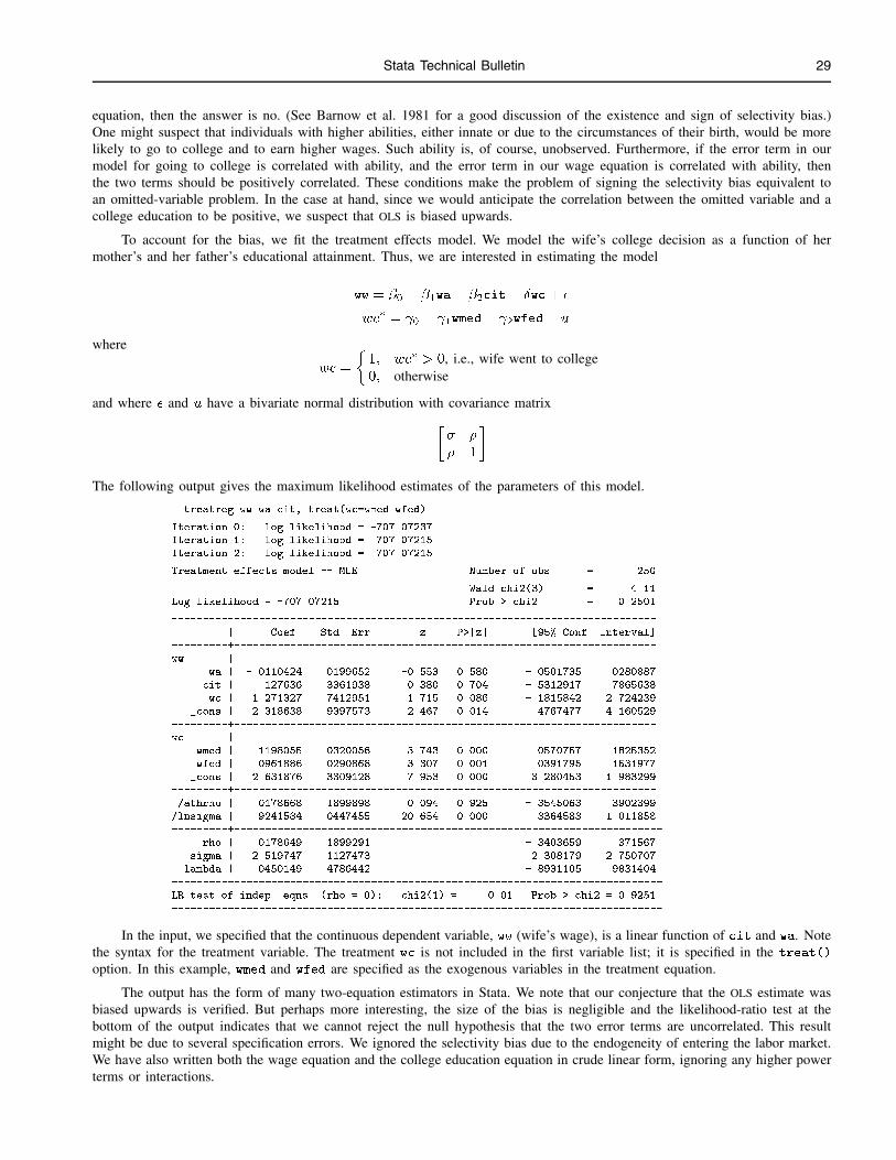
Stata Technical Bulletin 29
equation, then the answer is no. (See Barnow et al. 1981 for a good discussion of the existence and sign of selectivity bias.)One might suspect that individuals with higher abilities, either innate or due to the circumstances of their birth, would be morelikely to go to college and to earn higher wages. Such ability is, of course, unobserved. Furthermore, if the error term in ourmodel for going to college is correlated with ability, and the error term in our wage equation is correlated with ability, thenthe two terms should be positively correlated. These conditions make the problem of signing the selectivity bias equivalent toan omitted-variable problem. In the case at hand, since we would anticipate the correlation between the omitted variable and acollege education to be positive, we suspect that OLS is biased upwards.
To account for the bias, we fit the treatment effects model. We model the wife’s college decision as a function of hermother’s and her father’s educational attainment. Thus, we are interested in estimating the model
ww = �0 + �1wa+ �2cit+ �wc+ �
wc� = 0 + 1wmed+ 2wfed+ u
where
wc =
�1; wc
�> 0, i.e., wife went to college
0; otherwise
and where � and u have a bivariate normal distribution with covariance matrix�� �
� 1
�The following output gives the maximum likelihood estimates of the parameters of this model.
. treatreg ww wa cit, treat(wc=wmed wfed)
Iteration 0: log likelihood = -707.07237
Iteration 1: log likelihood = -707.07215
Iteration 2: log likelihood = -707.07215
Treatment effects model -- MLE Number of obs = 250
Wald chi2(3) = 4.11
Log likelihood = -707.07215 Prob > chi2 = 0.2501
------------------------------------------------------------------------------
| Coef. Std. Err. z P>|z| [95% Conf. Interval]
---------+--------------------------------------------------------------------
ww |
wa | -.0110424 .0199652 -0.553 0.580 -.0501735 .0280887
cit | .127636 .3361938 0.380 0.704 -.5312917 .7865638
wc | 1.271327 .7412951 1.715 0.086 -.1815842 2.724239
_cons | 2.318638 .9397573 2.467 0.014 .4767477 4.160529
---------+--------------------------------------------------------------------
wc |
wmed | .1198055 .0320056 3.743 0.000 .0570757 .1825352
wfed | .0961886 .0290868 3.307 0.001 .0391795 .1531977
_cons | -2.631876 .3309128 -7.953 0.000 -3.280453 -1.983299
---------+--------------------------------------------------------------------
/athrho | .0178668 .1899898 0.094 0.925 -.3545063 .3902399
/lnsigma | .9241584 .0447455 20.654 0.000 .8364588 1.011858
---------+---------------------------------------------------------------------
rho | .0178649 .1899291 -.3403659 .371567
sigma | 2.519747 .1127473 2.308179 2.750707
lambda | .0450149 .4786442 -.8931105 .9831404
-------------------------------------------------------------------------------
LR test of indep. eqns. (rho = 0): chi2(1) = 0.01 Prob > chi2 = 0.9251
-------------------------------------------------------------------------------
In the input, we specified that the continuous dependent variable, ww (wife’s wage), is a linear function of cit and wa. Notethe syntax for the treatment variable. The treatment wc is not included in the first variable list; it is specified in the treat()
option. In this example, wmed and wfed are specified as the exogenous variables in the treatment equation.
The output has the form of many two-equation estimators in Stata. We note that our conjecture that the OLS estimate wasbiased upwards is verified. But perhaps more interesting, the size of the bias is negligible and the likelihood-ratio test at thebottom of the output indicates that we cannot reject the null hypothesis that the two error terms are uncorrelated. This resultmight be due to several specification errors. We ignored the selectivity bias due to the endogeneity of entering the labor market.We have also written both the wage equation and the college education equation in crude linear form, ignoring any higher powerterms or interactions.

30 Stata Technical Bulletin STB-55
The results for the two ancillary parameters require explanation. For numerical stability during optimization, treatregdoes not directly estimate � or �. Instead, treatreg estimates the inverse hyperbolic tangent of �,
atanh � =1
2ln
�1 + �
1� �
�and ln�. Also, treatreg reports � = ��, along with an estimate of the standard error of the estimate and a confidence intervalfor it.
Technical Note
If each of the equations in the model had contained many regressors, the treatreg command could become quite long. Analternate way of specifying our wage model would be to make use of Stata’s local macros. The following lines are an equivalentway of estimating our model.
. local wageeq "ww wa cit"
. local trteq "wc=wmed wfed"
. treatreg `wageeq', treat(`trteq')
Example (continued)
Stata will also produce a two-step estimator of the model with the twostep option. Maximum likelihood estimation of theparameters can be time-consuming with large datasets, and the two-step estimates may provide a good alternative in such cases.Continuing with the women’s wage model, we can obtain the two-step estimates with consistent covariance estimates by typing
. treatreg ww wa cit, treat(wc=wmed wfed) twostep
Treatment effects model -- two-step estimates Number of obs = 250
Wald chi2(3) = 3.67
Prob > chi2 = 0.2998
------------------------------------------------------------------------------
| Coef. Std. Err. z P>|z| [95% Conf. Interval]
---------+--------------------------------------------------------------------
ww |
wa | -.0111623 .020152 -0.554 0.580 -.0506594 .0283348
cit | .1276102 .33619 0.380 0.704 -.53131 .7865305
wc | 1.257995 .8007428 1.571 0.116 -.3114319 2.827422
_cons | 2.327482 .9610271 2.422 0.015 .4439031 4.21106
---------+--------------------------------------------------------------------
wc |
wmed | .1198888 .0319859 3.748 0.000 .0571976 .1825801
wfed | .0960764 .0290581 3.306 0.001 .0391236 .1530292
_cons | -2.631496 .3308344 -7.954 0.000 -3.279919 -1.983072
---------+--------------------------------------------------------------------
hazard |
lambda | .0548738 .5283928 0.104 0.917 -.9807571 1.090505
------------------------------------------------------------------------------
rho | 0.02178
sigma | 2.5198211
lambda | .05487379 .5283928
-------------------------------------------------------------------------------
The reported lambda (�) is the parameter estimate on the hazard from the augmented regression. The augmented regressionis derived in Maddala (1983) and presented in the Methods and Formulas section below.
The default statistic produced by predict after treatreg is the expected value of the dependent variable from theunderlying distribution of the regression model. For the case at hand this statistic is
ww = �0 + �1wa+ �2cit+ �wc+ �
Several other interesting aspects of the treatment effects model can be explored with predict. Continuing with our wagemodel, the wife’s expected wage, conditional on attending college, can be obtained with the yctrt option. The wife’s expectedwages, conditional on not attending college, can be obtained with the ycntrt option. Thus, the difference in expected wagesbetween participants and nonparticipants is the difference between yctrt and ycntrt. For the case at hand, we have thefollowing calculation:
. predict wwctrt, yctrt

Stata Technical Bulletin 31
. predict wwcntrt, ycntrt
. gen diff = wwctrt - wwcntrt
. summarize diff
Variable | Obs Mean Std. Dev. Min Max
---------+-----------------------------------------------------
diff | 250 1.356912 .0134202 1.34558 1.420173
Technical Note
The difference in expected earnings between participants and nonparticipants is
E [yi j zi = 1]� E [yi j zi = 0] = � + ��
��i
�i (1� �i)
�If the correlation between the error terms, �, is zero, then the problem reduces to one estimable by OLS and the difference issimply �. Since � is positive in our example, we see that least squares overestimates the treatment effect.
Saved Results
treatreg saves in e():
Scalarse(N) number of observations e(selambda) standard error of �e(k) number of variables e(rc) return codee(k eq) number of equations e(sigma) �
e(k dv) number of dependent variables e(chi2) �2
e(df m) model degrees of freedom e(chi2 c) �2 for comparison teste(ll) log likelihood e(p c) p-value for comparison teste(p) p-value for �2 test e(rho) �
e(N clust) number of clusters e(ic) number of iterationse(lambda) �
Macrose(cmd) treatreg e(user) name of likelihood-evaluator programe(depvar) name(s) of dependent variable(s) e(opt) type of optimizatione(title) title in estimation output e(chi2type) Wald or LR; type of model �2 teste(clustvar) name of cluster variable e(chi2 ct) Wald or LR; type of model �2 teste(wtype) weight type corresponding to e(chi2 c)
e(wexp) weight expression e(hazard) variable containing hazarde(method) requested estimation method e(predict) program used to implement predicte(vcetype) covariance estimation method
Matricese(b) coefficient vector e(V) variance–covariance matrix of the
estimators
Functionse(sample) marks estimation sample
Methods and Formulas
treatreg is implemented as an ado-file. Maddala (1983, 117–122) derives both the maximum likelihood and the two-stepestimator implemented here. Greene (2000, 933–934) also provides an introduction to the treatment effects model.
The primary regression equation of interest isyj = xj� + �zj + �j
where zj is a binary decision variable. The binary variable is assumed to stem from an unobservable latent variable
z�j = wj + uj
The decision to obtain the treatment is made according to the rule
zj =
�1; if z�j > 00; otherwise

32 Stata Technical Bulletin STB-55
where � and u are bivariate normal with mean zero and covariance matrix�� �
� 1
�
The likelihood function for this model is given in Maddala (1983, 122). Greene (2000, 180) discusses the standard methodof reducing a bivariate normal to a function of a univariate normal and the correlation �. Combining the two yields the followinglog likelihood for observation j:
lj =
8>>>>>><>>>>>>:ln�
wj + (yj � xj� � �)�=�p
1� �2
!� 1
2
�yj � xj� � �
�
�2
� ln(p2��) zj = 1
ln�
�wj � (yj � xj�)�=�p
1� �2
!� 1
2
�yj � xj�
�
�2
� ln(p2��) zj = 0
where �() is the distribution function of the standard normal distribution.
In the maximum likelihood estimation, � and � are not directly estimated. Directly estimated are ln� and atanh �, where
atanh � =1
2ln
�1 + �
1� �
�The standard error of � = �� is approximated through the propagation of error (delta) method, which is given by
Var(�) � DVar�[atanh � ln�]
�D0
where D is the Jacobian of � with respect to atanh � and ln�.
Maddala (1983, 120–122), also derives the two-step estimator. In the first stage, one obtains probit estimates of the treatmentequation
Pr(zj = 1 j wj) = �(wj )
From these estimates the hazard, hj , for each observation j is computed as
hj =
8>>>><>>>>:�(wjb )�(wjb ) zj = 1
��(wjb )1� �(wjb ) zj = 0
where � is the standard normal density function. We also define
dj = hj(hj + b wj)
Then,E [yi j zi] = Xj� + �zj + ��hj
Var [yi j zi] = �2�1� �
2dj
�The two-step parameter estimates of � and � are obtained by augmenting the regression equation with the hazard h. Thus,
the regressors become [X z h ] and we obtain the additional parameter estimate �h on the variable containing the hazard. Aconsistent estimate of the regression disturbance variance is obtained using the residuals from the augmented regression and theparameter estimate on the hazard
b�2 = e0e+ �2h
PNj=1 dj
N
The two-step estimate of � is then b� = �hb�
Stata Technical Bulletin 33
We will now describe how the consistent estimates of the coefficient covariance matrix based on the augmented regressionare derived. Let A = [X Z h ] and D be a square diagonal matrix of rank N with (1� b� 2
dj) on the diagonal elements.
Vtwostep = b�2(A0A)�1(A0DA+Q)(A0A)�1
whereQ = b� 2(A0DA)Vp(A
0DA)
and Vp is the variance–covariance estimate from the probit estimation of the treatment equation.
ReferenceBarnow, B., G. Cain, and A. Goldberger. 1981. Issues in the analysis of selectivity bias. Evaluation Studies Review Annual 5. Beverly Hills: Sage
Publications.
Berndt, E. 1991. The Practice of Econometrics. New York: Addison–Wesley.
Greene, W. H. 2000. Econometric Analysis. 4th ed. Upper Saddle River, NJ: Prentice–Hall.
Maddala, G. S. 1983. Limited-dependent and Qualitative Variables in Econometrics. Cambridge, UK: Cambridge University Press.
sg142 Uniform layer effect models for the analysis of differences in two-way associations
Maurizio Pisati, University of Trento, Italy, [email protected]
Abstract: Many relevant research questions pertain to how the association between two categorical variables (say R and C)depends on the values taken on by a third categorical variable (say L). The uniform layer effect models illustrated in thisinsert represent a particular way to tackle these questions. Specifically, they are a variety of the standard loglinear modelbased on three assumptions: a) there is an association between variables R and C, b) the pattern of association between Rand C is constant across the categories of variable L, and c) the strength of association between R and C varies betweenany pair of categories of L by a uniform amount. This insert focuses on two different specifications of the uniform layereffect model: Yamaguchi’s additive model and Xie’s multiplicative model.
Keywords: Contingency table analysis, mobility table analysis, loglinear model, additive model, multiplicative model.
Overview
Many relevant research questions pertain to how the association between two categorical variables (say R and C) dependson the values taken on by a third categorical variable (say L). To tackle these questions, we first arrange the data into a three-waycontingency table, whose cell frequencies can be expressed in terms of the standard saturated loglinear model
log(Fijk) = �+ �Ri + �
Cj + �
Lk + �
RLik + �
CLjk + �
RCij + �
RCLijk
where log(Fijk) denotes the natural logarithm of the expected frequency in cell (i; j; k), i indexes the I categories of the rowvariable R, j indexes the J categories of the column variable C, k indexes the K categories of the layer variable L, and the �parameters are subject to a standard set of constraints that make them identifiable (Powers and Xie 2000).
When dealing with the kind of questions mentioned above, the researcher typically focuses on the specification of both thetwo-way interaction term which expresses the baseline pattern of association between variables R and C, and the three-wayinteraction term which expresses how the R by C association observed in each layer k departs from that baseline pattern. Thereare many ways to specify �RCij and �RCLijk , all of which can be seen as lying on a continuum whose extremes correspond on
the one hand to the conditional independence model, which sets �RCij = �RCLijk = 0 for all combinations of i, j, and k, and
on the other hand to the saturated model, which specifies the association between R and C conditional on L using all the(I � 1)� (J � 1)�K available degrees of freedom.
The uniform layer effect models illustrated in this insert represent a particular way to specify the interaction terms �RCij and�RCLijk (Goodman and Hout 1998). In their standard formulation, the models belonging to this category share three assumptions:
� There is an association between variables R and C, that is, �RCij 6= 0.
� The pattern of association between variables R and C, as represented by the fundamental set of (conditional) log-odds ratioslog(�ijjk) = log(Fijk) + log(F(i+1)(j+1)k)� log(F(i+1)jk)� log(Fi(j+1)k) for i = 1; : : : ; I � 1 and j = 1; : : : ; J � 1is constant across layers.
� The strength of association between variables R and C varies between any pair of layers by a uniform amount.

34 Stata Technical Bulletin STB-55
This insert focuses on two different specifications of the uniform layer effect model: the additive model and the multiplicativemodel. The additive model has been proposed by Yamaguchi (1987) and can be formulated as
log(Fijk) = �+ �Ri + �
Cj + �
Lk + �
RLik + �
CLjk + �
RCij + ij�k
where the � and � parameters are subject to appropriate constraints that make them identifiable. As we can see, the additivemodel retains the two-way interaction term but replaces the three-way interaction term with the product ij�k. This means thatthe conditional log-odds ratios pertaining to each layer k take the parametric form
log(�ijjk) = �RCij + �
RC(i+1)(j+1) � �
RC(i+1)j � �
RCi(j+1) + �k
Hence, in the additive model the � parameters express the extent to which the strength of the association between variablesR and C varies across layers. More precisely, the difference between any pair of � parameters (say �k and �k� ) expresses inabsolute terms how much the R by C association is uniformly stronger or weaker in layer k than in layer k� (Goodman andHout 1998, 184). Formally,
�k�k� = log(�ijjk)� log(�ijjk�) = �k � �k� ; i = 1; : : : ; I � 1; j = 1; : : : ; J � 1
It should be noted that because of the presence of the ij product in the equation, the results produced by the additive modeldepend on the ordering of both the row and column categories (Goodman and Hout 1998, 184).
Sometimes the layers can be assigned exogenous scores that have a theoretical meaning (Yamaguchi 1987, 486). In suchcases, the additive model can be reformulated as
log(Fijk) = �+ �Ri + �
Cj + �
Lk + �
RLik + �
CLjk + �
RCij +
VXv=1
ijSvk�v
where v indexes the V exogenous scores assigned to the layers, Svk denotes the value taken on by score v in layer k, and �vdenotes the linear effect exerted by score v on the log-odds ratios. Thus, according to this version of the additive model, whichI will refer to as the linear additive model, the difference between any pair of conditional log-odds ratios pertaining to layers kand k� is equal to
�k�k� = log(�ijjk)� log(�ijjk�) =
VXv=1
(Svk � Svk�)�v; i = 1; : : : ; I; j = 1; : : : ; J
It should be noted that in most cases, to ensure both identification and meaningfulness of the � parameters, it is required thatV � K � 2.
The multiplicative model has been proposed by Xie (1992), see also Erikson and Goldthorpe (1992, 91–93) and can beformulated as
log(Fijk) = �+ �Ri + �
Cj + �
Lk + �
RLik + �
CLjk + ij�k
where the �, , and � parameters are subject to appropriate constraints that make them identifiable. As we can see, themultiplicative model replaces both the two-way interaction term �
RCij and the three-way interaction term �
RCLijk with the product
ij�k, where ij denotes cell-specific scores that express the baseline pattern of association between variables R and C, and�k denotes layer-specific scores that express the strength of the R by C association in each layer. The and � parameters canbe seen as latent scores estimated from the data using iterative procedures (Xie 1992, 382; Goodman and Hout 1998, 181–182).
The formula for the multiplicative model implies that the conditional log-odds ratios pertaining to each layer k take theparametric form
log(�ijjk) = ( ij + (i+1)(j+1) � (i+1)j � i(j+1))�k
Consequently, in the multiplicative model the ratio between any pair of � parameters (say �k and ��k) expresses in relative termshow much the association between variables R and C is uniformly stronger or weaker in layer k than in layer k� (Goodmanand Hout 1998, 185). Formally,
�k=k� = log(�ijjk)= log(�ijjk�) = �k=�k� ; i = 1; : : : ; I � 1; j = 1; : : : ; J � 1
Both the additive and the multiplicative uniform layer effect models have been originally devised to compare social mobilitytables across countries or over time. However, both models can be applied to any research question where the R by C associationis assumed to have the same pattern but possibly different strengths across layers (see Xie 1991, Goodman and Hout 1998).
Stata Technical Bulletin 35
Syntax
unidiff cellvar , row(rowvar) column(colvar) layer(layvar) effect(null j add j addlin j mult)pattern(fi j qpm j qs j cp j ua j re j ce j rce j hrce j own1 j own2) � quasi
design(varlist) scores(varlist) extra(varlist) refcat(#) constraints(numlist)
lambda(rawlog j rawexp j stdlog j stdexp) shd(log j exp) saveexp(newvar)
savelambda(newvar) nodetail nodisprc nodispextra�
Description
unidiff estimates the null, additive, linear additive, and multiplicative uniform layer effect models, displays relevantgoodness-of-fit statistics and parameter estimates, and optionally computes several ancillary quantities of interest. The dataset tobe analyzed must include at least four variables:
� cellvar contains the observed cell frequencies that make up the three-way contingency table object of analysis.
� rowvar indexes (and optionally labels) the I categories of the row variable.
� colvar indexes (and optionally labels) the J categories of the column variable.
� layvar indexes (and optionally labels) the K categories of the layer variable.
Note that unidiff drops without warning all variables starting with rc .
Options
row(rowvar) is required. It specifies the name of the row variable.
column(colvar) is required. It specifies the name of the column variable.
layer(layvar) is required. It specifies the name of the layer variable.
effect(null j add j addlin j mult) is required. It specifies the type of uniform layer effect model to be estimated.
effect(null) estimates the null effect model, that is, a model that postulates constant pattern and strength of the R byC association across layers.
effect(add) estimates the additive model.
effect(addlin) estimates the linear additive model.
effect(mult) estimates the multiplicative model.
pattern(fi j qpm j qs j cp j ua j re j ce j rce j hrce j own1 j own2) is required. It specifies the baseline pattern ofassociation between variables R and C , that is, the form taken by the two-way interaction term �
RCij or, in the case of the
multiplicative model, by the ij parameters. Some patterns are allowed only when I = J . For details on all these patternsof association, see Hout (1983).
pattern(fi) specifies the “full interaction” (saturated) pattern of association.
pattern(qpm) specifies the “quasi-perfect mobility” pattern of association. It is allowed only when I = J .
pattern(qs) specifies the “quasi-symmetry” pattern of association. It is allowed only when I = J .
pattern(cp) specifies the “crossing parameters” pattern of association. It is allowed only when I = J .
pattern(ua) specifies the “uniform association” pattern of association.
pattern(re) specifies the “row effects” pattern of association.
pattern(ce) specifies the “column effects” pattern of association.
pattern(rce) specifies the “row and column effects I” pattern of association.
pattern(hrce) specifies the “homogeneous row and column effects I” pattern of association. It is allowed only whenI = J .
pattern(own1) specifies a user-defined pattern of association expressed by a single “topological,” that is, categoricalvariable.
pattern(own2) specifies a user-defined pattern of association expressed by one or more quantitative variables.

36 Stata Technical Bulletin STB-55
quasi requires that the “quasi-version” (i.e., with diagonal-specific parameters) of the selected pattern of the R by C associationbe applied. It is allowed only when I = J .
design(varlist) is required if pattern(own1) or pattern(own2) is specified. It specifies the list of variables that expressesthe user-defined baseline pattern of association between variables R and C.
extra(varlist) specifies a list of additional variables intended to express particular features of the model that lie outside itsstandard formulation. When this option is specified, the formulas for the additive, linear-additive and multiplicative-uniformlayer effect models reported above must be complemented with the term
PT
t=1 �txtijk, where t indexes the T “extra”variables included in the model, xtijk denotes the value taken on by “extra” variable t in cell (i; j; k), and �t denotes theparameter associated with the “extra” variable t.
scores(varlist) is required if effect(addlin) is specified. It specifies the list of variables that represent the V exogenousscores assigned to the layers.
refcat(#) specifies the layer to be taken as the reference category in the estimation of parameters �k or �k. For identificationpurposes, the following constraints are imposed: �r = 0 for the additive model, and �r = 1 for the multiplicative model,where r is the index specified by refcat. By default, layer 1 is taken as the reference category.
constraints(numlist) specifies equality constraints to be imposed on the estimation of parameters �k or �k. Suppose we areanalyzing a table with four layers and want to make �1 = �2. To impose this equality restriction we specify constraints (11 2 3).
lambda(rawlog j rawexp j stdlog j stdexp) displays in tabular form the total interaction effects estimated by the fittedmodel for each layer, that is, the equivalent of the sum �
RCij + �
RCLijk for all combinations of i, j, and k.
lambda(rawlog) displays the raw effects in additive (logarithmic) form (�ijjk).
lambda(rawexp) displays the raw effects in multiplicative (exponential) form (exp(�ijjk)).
lambda(stdlog) displays the standardized effects in additive form (~�ijjk). Standardization is achieved by “double-centering”the effects around their mean, so that within each row, column, and layer they sum to zero (see Goodman 1991, 1088).
lambda(stdexp) displays the standardized effects in multiplicative form (exp(~�ijjk)).
shd(log j exp) displays in tabular form layer-specific structural shift parameters (with standard errors), structural distances (withstandard errors), mean structural distances, and overall structural effect computed according to the Sobel–Hout–Duncanapproach to mobility table modeling (Sobel, et al. 1985). These quantities are particularly relevant in the analysis of socialmobility tables and can be computed only when I = J .
shd(log) displays all the above quantities in additive (logarithmic) form.
shd(exp) displays all the above quantities in multiplicative (exponential) form.
saveexp(newvar) creates newvar containing the expected cell frequencies under the fitted model.
savelambda(newvar) creates newvar containing the total interaction effects estimated by the fitted model. The effects are savedin standardized additive form (~�ijjk).
nodetail suppresses the output describing the structure of the contingency table object of analysis and the specification of thefitted model.
nodisprc suppresses the output of the table reporting the parameter estimates associated with the variables that express the Rby C association pattern.
nodispextra suppresses the output of the table reporting the parameter estimates associated with the extra variables.
Example 1
In this first example, I reanalyze the social mobility data used by Yamaguchi (1987) and Xie (1992) in their illustration of,respectively, the additive and the multiplicative uniform layer effect models. It is a 5�5�3 contingency table that cross-classifiesfather’s occupational class (the row variable), son’s occupational class (the column variable), and country (the layer variable).The pattern of association between father’s class and son’s class is assumed to be constant across countries. The purpose of theanalysis is to detect any cross-national variation in the strength of the father-son association.
. use example1.dta, clear
. describe

Stata Technical Bulletin 37
Contains data from example1.dta
obs: 75
vars: 4
size: 675 (97.5% of memory free)
-------------------------------------------------------------------------------
1. obs int %8.0g Observed cell frequencies
2. country byte %13.0g country Country
3. father byte %15.0g class Father's occupational class
4. son byte %15.0g class Son's occupational class
-------------------------------------------------------------------------------
Sorted by:
. label list
country:
1 United States
2 Britain
3 Japan
class:
1 UpNonManual
2 LowNonManual
3 UpManual
4 LowManual
5 Farm
Let us start with the additive model. To reproduce Yamaguchi’s (1987) results, two assumptions must be taken into account.First, occupational classes are ordered hierarchically along a vertical status dimension ranging from upper nonmanual (highest)to farm (lowest). Second, models are applied to off-diagonal cells only, due to the particular meaning that diagonal cells have inmobility table analysis. This means that diagonal cells must be “blocked,”, that is, their frequencies must be exactly reproducedby the models. To this aim, we must create and include in the models as “extra” variables, 15 (= I �K) indicator variables,one for each diagonal cell of each layer.
. local COUNTRY "US GB JA"
. local i=1
. while `i'<=3 {
2. local ITEM : word `i' of `COUNTRY'
3. local j=1
4. while `j'<=5 {
5. generate diag`i'`j'=country==`i' & father==`j' & son==`j'
6. lab var diag`i'`j' "`ITEM': Immobility in class `j'"
7. local j=`j'+1
8. }
9. local i=`i'+1
10. }
. describe
Contains data from example1.dta
obs: 75
vars: 19
size: 5,175 (97.5% of memory free)
-------------------------------------------------------------------------------
1. obs int %8.0g Observed cell frequencies
2. country byte %13.0g country Country
3. father byte %15.0g class Father's occupational class
4. son byte %15.0g class Son's occupational class
5. diag11 float %9.0g US: Immobility in class 1
6. diag12 float %9.0g US: Immobility in class 2
7. diag13 float %9.0g US: Immobility in class 3
8. diag14 float %9.0g US: Immobility in class 4
9. diag15 float %9.0g US: Immobility in class 5
10. diag21 float %9.0g GB: Immobility in class 1
11. diag22 float %9.0g GB: Immobility in class 2
12. diag23 float %9.0g GB: Immobility in class 3
13. diag24 float %9.0g GB: Immobility in class 4
14. diag25 float %9.0g GB: Immobility in class 5
15. diag31 float %9.0g JA: Immobility in class 1
16. diag32 float %9.0g JA: Immobility in class 2
17. diag33 float %9.0g JA: Immobility in class 3
18. diag34 float %9.0g JA: Immobility in class 4
19. diag35 float %9.0g JA: Immobility in class 5
-------------------------------------------------------------------------------
Sorted by:
In his analysis, Yamaguchi (1987) tests several specifications of the pattern of association between father’s class and son’s

38 Stata Technical Bulletin STB-55
class. For illustration purposes, I will focus on two of them; the “full interaction” pattern and the “homogeneous row and columneffects” pattern. The additive model with full interaction pattern of the R by C association and “blocked” diagonal cells can beestimated by
. unidiff obs, row(father) col(son) lay(country) effect(add) pattern(fi)
> extra(diag11-diag35)
Analysis of differences in two-way associations
Table structure
-------------------------------------------------------------------------------
Name Label N. of categories
-------------------------------------------------------------------------------
Row father Father's occupational class 5
Column son Son's occupational class 5
Layer country Country 3
-------------------------------------------------------------------------------
Model specification
-------------------------------------------------------------------------------
Layer effect: additive
R-C association pattern: full interaction
Additional variables: diag11 diag12 diag13 diag14 diag15 diag21
diag22 diag23 diag24 diag25 diag31 diag32
diag33 diag34 diag35
-------------------------------------------------------------------------------
Goodness-of-fit statistics
-------------------------------------------------------------------------------
Model N df X2 p G2 p rG2 BIC DI
-------------------------------------------------------------------------------
Cond. indep. 28887 48 6659.6 0.00 5591.5 0.00 0.0 5098.5 16.0
Null effect 28887 22 36.2 0.03 36.2 0.03 99.4 -189.7 0.9
Additive effect 28887 20 30.7 0.06 30.7 0.06 99.5 -174.7 0.7
-------------------------------------------------------------------------------
Beta parameters
--------------+-----------------------------------
Country | estimate s.e. p-value
--------------+-----------------------------------
United States | 0.0000 0.0000 0.0000
Britain | 0.0035 0.0147 0.8133
Japan | -0.0411 0.0180 0.0227
--------------+-----------------------------------
R-C association parameters
--------------------------------------------------------------------------
Variable Label estimate s.e. p-value
--------------------------------------------------------------------------
rc_fi2 Full interaction: level 2 -3.1828 0.2629 0.0000
rc_fi3 Full interaction: level 3 -3.1345 0.2618 0.0000
rc_fi4 Full interaction: level 4 -3.0926 0.2598 0.0000
rc_fi5 Full interaction: level 5 -3.3612 0.2348 0.0000
rc_fi6 Full interaction: level 6 -3.2003 0.2598 0.0000
rc_fi7 Full interaction: level 7 -1.6144 0.2949 0.0000
rc_fi8 Full interaction: level 8 -2.3159 0.2541 0.0000
rc_fi9 Full interaction: level 9 -2.8696 0.2285 0.0000
rc_fi10 Full interaction: level 10 -3.0470 0.2584 0.0000
rc_fi11 Full interaction: level 11 -2.0611 0.2552 0.0000
rc_fi12 Full interaction: level 12 -1.6946 0.2556 0.0000
rc_fi13 Full interaction: level 13 -2.7080 0.2261 0.0000
rc_fi14 Full interaction: level 14 -2.9291 0.2545 0.0000
rc_fi15 Full interaction: level 15 -1.8084 0.2493 0.0000
rc_fi16 Full interaction: level 16 -1.3609 0.2445 0.0000
rc_fi17 Full interaction: level 17 0.0000 0.0000 0.0000
--------------------------------------------------------------------------
Extra variable parameters
--------------------------------------------------------------------------
Variable Label estimate s.e. p-value
--------------------------------------------------------------------------
diag11 US: Immobility in class 1 3.8151 0.2524 0.0000
diag12 US: Immobility in class 2 0.0000 0.0000 0.0000
diag13 US: Immobility in class 3 -0.5863 0.1402 0.0000
diag14 US: Immobility in class 4 0.0235 0.0690 0.7334
diag15 US: Immobility in class 5 0.2605 0.2189 0.2340
diag21 GB: Immobility in class 1 4.0496 0.2775 0.0000
diag22 GB: Immobility in class 2 0.1899 0.1024 0.0636
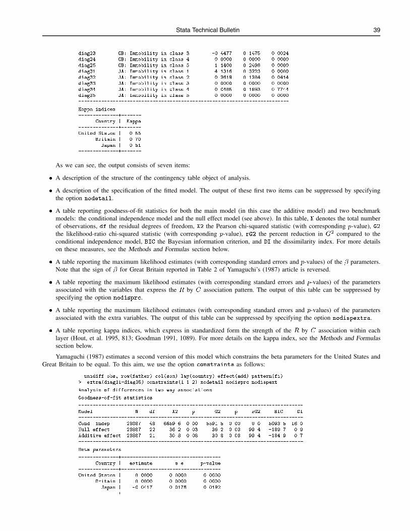
Stata Technical Bulletin 39
diag23 GB: Immobility in class 3 -0.4477 0.1475 0.0024
diag24 GB: Immobility in class 4 0.0000 0.0000 0.0000
diag25 GB: Immobility in class 5 1.1400 0.2498 0.0000
diag31 JA: Immobility in class 1 4.1316 0.3223 0.0000
diag32 JA: Immobility in class 2 0.2619 0.1284 0.0414
diag33 JA: Immobility in class 3 0.0000 0.0000 0.0000
diag34 JA: Immobility in class 4 -0.0485 0.1693 0.7744
diag35 JA: Immobility in class 5 0.0000 0.0000 0.0000
--------------------------------------------------------------------------
Kappa indices
--------------+-------
Country | Kappa
--------------+-------
United States | 0.55
Britain | 0.70
Japan | 0.51
--------------+-------
As we can see, the output consists of seven items:
� A description of the structure of the contingency table object of analysis.
� A description of the specification of the fitted model. The output of these first two items can be suppressed by specifyingthe option nodetail.
� A table reporting goodness-of-fit statistics for both the main model (in this case the additive model) and two benchmarkmodels: the conditional independence model and the null effect model (see above). In this table, N denotes the total numberof observations, df the residual degrees of freedom, X2 the Pearson chi-squared statistic (with corresponding p-value), G2the likelihood-ratio chi-squared statistic (with corresponding p-value), rG2 the percent reduction in G
2 compared to theconditional independence model, BIC the Bayesian information criterion, and DI the dissimilarity index. For more detailson these measures, see the Methods and Formulas section below.
� A table reporting the maximum likelihood estimates (with corresponding standard errors and p-values) of the � parameters.Note that the sign of � for Great Britain reported in Table 2 of Yamaguchi’s (1987) article is reversed.
� A table reporting the maximum likelihood estimates (with corresponding standard errors and p-values) of the parametersassociated with the variables that express the R by C association pattern. The output of this table can be suppressed byspecifying the option nodisprc.
� A table reporting the maximum likelihood estimates (with corresponding standard errors and p-values) of the parametersassociated with the extra variables. The output of this table can be suppressed by specifying the option nodispextra.
� A table reporting kappa indices, which express in standardized form the strength of the R by C association within eachlayer (Hout, et al. 1995, 813; Goodman 1991, 1089). For more details on the kappa index, see the Methods and Formulassection below.
Yamaguchi (1987) estimates a second version of this model which constrains the beta parameters for the United States andGreat Britain to be equal. To this aim, we use the option constraints as follows:
. unidiff obs, row(father) col(son) lay(country) effect(add) pattern(fi)
> extra(diag11-diag35) constraints(1 1 2) nodetail nodisprc nodispext
Analysis of differences in two-way associations
Goodness-of-fit statistics
-------------------------------------------------------------------------------
Model N df X2 p G2 p rG2 BIC DI
-------------------------------------------------------------------------------
Cond. indep. 28887 48 6659.6 0.00 5591.5 0.00 0.0 5098.5 16.0
Null effect 28887 22 36.2 0.03 36.2 0.03 99.4 -189.7 0.9
Additive effect 28887 21 30.8 0.08 30.8 0.08 99.4 -184.9 0.7
-------------------------------------------------------------------------------
Beta parameters
--------------+-----------------------------------
Country | estimate s.e. p-value
--------------+-----------------------------------
United States | 0.0000 0.0000 0.0000
Britain | 0.0000 0.0000 0.0000
Japan | -0.0417 0.0178 0.0192
--------------+-----------------------------------

40 Stata Technical Bulletin STB-55
Kappa indices
--------------+-------
Country | Kappa
--------------+-------
United States | 0.55
Britain | 0.70
Japan | 0.51
--------------+-------
Let us consider now the “homogeneous row and column effects” specification of the pattern of association between father’sclass and son’s class. To specify this pattern within unidiff, we have
. unidiff obs, row(father) col(son) lay(country) effect(add) pattern(hrce)
> extra(diag11-diag35) nodispext
Analysis of differences in two-way associations
Table structure
-------------------------------------------------------------------------------
Name Label N. of categories
-------------------------------------------------------------------------------
Row father Father's occupational class 5
Column son Son's occupational class 5
Layer country Country 3
-------------------------------------------------------------------------------
Model specification
-------------------------------------------------------------------------------
Layer effect: additive
R-C association pattern: homogeneous row & column effects I
Additional variables: diag11 diag12 diag13 diag14 diag15 diag21
diag22 diag23 diag24 diag25 diag31 diag32
diag33 diag34 diag35
-------------------------------------------------------------------------------
Goodness-of-fit statistics
-------------------------------------------------------------------------------
Model N df X2 p G2 p rG2 BIC DI
-------------------------------------------------------------------------------
Cond. indep. 28887 48 6659.6 0.00 5591.5 0.00 0.0 5098.5 16.0
Null effect 28887 29 125.5 0.00 107.0 0.00 98.1 -190.9 1.3
Additive effect 28887 27 117.2 0.00 98.4 0.00 98.2 -179.0 1.2
-------------------------------------------------------------------------------
Beta parameters
--------------+-----------------------------------
Country | estimate s.e. p-value
--------------+-----------------------------------
United States | 0.0000 0.0000 0.0000
Britain | -0.0025 0.0148 0.8657
Japan | -0.0524 0.0178 0.0034
--------------+-----------------------------------
R-C association parameters
--------------------------------------------------------------------------
Variable Label estimate s.e. p-value
--------------------------------------------------------------------------
rc_rc2 Row-Column effect 2 0.1012 0.0329 0.0021
rc_rc3 Row-Column effect 3 0.2729 0.0250 0.0000
rc_rc4 Row-Column effect 4 0.3333 0.0258 0.0000
rc_rc5 Row-Column effect 5 0.3323 0.0227 0.0000
--------------------------------------------------------------------------
Kappa indices
--------------+-------
Country | Kappa
--------------+-------
United States | 0.62
Britain | 0.77
Japan | 0.52
--------------+-------
The multiplicative version of the uniform layer effect model with full interaction pattern of the R by C association and“blocked” diagonal cells can be estimated by
. unidiff obs, row(father) col(son) lay(country) effect(mult) pattern(fi)
> extra(diag11-diag35) nodispext

Stata Technical Bulletin 41
Iteration 1: deviance = 53.4755
Iteration 2: deviance = 35.3281
Iteration 3: deviance = 0.6868
Iteration 4: deviance = 0.0206
Iteration 5: deviance = 0.0009
Iteration 6: deviance = 0.0000
Analysis of differences in two-way associations
Table structure
-------------------------------------------------------------------------------
Name Label N. of categories
-------------------------------------------------------------------------------
Row father Father's occupational class 5
Column son Son's occupational class 5
Layer country Country 3
-------------------------------------------------------------------------------
Model specification
-------------------------------------------------------------------------------
Layer effect: multiplicative
R-C association pattern: full interaction
Additional variables: diag11 diag12 diag13 diag14 diag15 diag21
diag22 diag23 diag24 diag25 diag31 diag32
diag33 diag34 diag35
-------------------------------------------------------------------------------
Goodness-of-fit statistics
-------------------------------------------------------------------------------
Model N df X2 p G2 p rG2 BIC DI
-------------------------------------------------------------------------------
Cond. indep. 28887 48 6659.6 0.00 5591.5 0.00 0.0 5098.5 16.0
Null effect 28887 22 36.2 0.03 36.2 0.03 99.4 -189.7 0.9
Multipl. effect 28887 20 30.7 0.06 30.9 0.06 99.4 -174.5 0.7
-------------------------------------------------------------------------------
Phi parameters (layer scores)
--------------+-----------------------------------
Country | Raw Scaled 1 Scaled 2
--------------+-----------------------------------
United States | 1.7025 1.0000 0.6064
Britain | 1.7703 1.0398 0.6305
Japan | 1.3605 0.7991 0.4845
--------------+-----------------------------------
Psi parameters (R-C association scores)
-------------+---------------------------------------
Father's |
occupational | Son's occupational class
class | UpNonM LowNon UpManu LowMan Farm
-------------+---------------------------------------
UpNonManual | 0.00 0.00 0.00 0.00 0.00
LowNonManual | 0.00 0.59 0.51 0.54 0.37
UpManual | 0.00 0.48 1.14 0.99 0.64
LowManual | 0.00 0.57 1.14 1.35 0.73
Farm | 0.00 0.64 1.29 1.55 2.93
-------------+---------------------------------------
Kappa indices
--------------+-------
Country | Kappa
--------------+-------
United States | 0.55
Britain | 0.70
Japan | 0.51
--------------+-------
As we can see, the output includes two new items:
� A table reporting the maximum likelihood estimates of the � parameters (layer scores). Three series of � parameters arereported: raw estimates, estimates rescaled so that �r = 1, and estimates rescaled so that
PKk=1 �
2k = 1 (see Xie 1992,
382).
� A table reporting the maximum likelihood estimates of the parameters (R by C association scores).
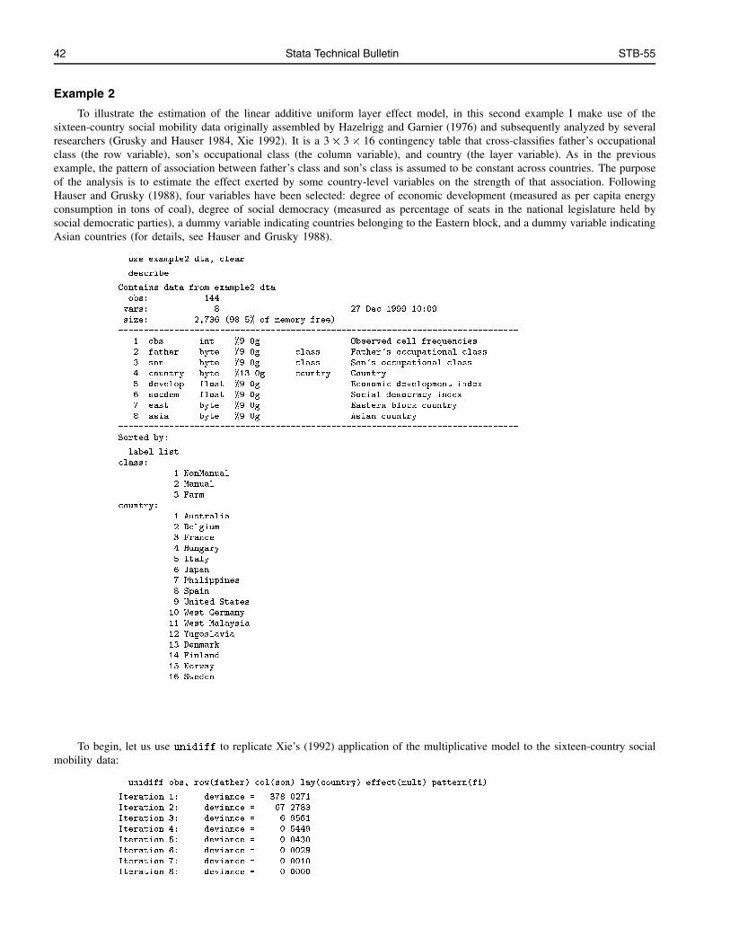
42 Stata Technical Bulletin STB-55
Example 2
To illustrate the estimation of the linear additive uniform layer effect model, in this second example I make use of thesixteen-country social mobility data originally assembled by Hazelrigg and Garnier (1976) and subsequently analyzed by severalresearchers (Grusky and Hauser 1984, Xie 1992). It is a 3� 3� 16 contingency table that cross-classifies father’s occupationalclass (the row variable), son’s occupational class (the column variable), and country (the layer variable). As in the previousexample, the pattern of association between father’s class and son’s class is assumed to be constant across countries. The purposeof the analysis is to estimate the effect exerted by some country-level variables on the strength of that association. FollowingHauser and Grusky (1988), four variables have been selected: degree of economic development (measured as per capita energyconsumption in tons of coal), degree of social democracy (measured as percentage of seats in the national legislature held bysocial democratic parties), a dummy variable indicating countries belonging to the Eastern block, and a dummy variable indicatingAsian countries (for details, see Hauser and Grusky 1988).
. use example2.dta, clear
. describe
Contains data from example2.dta
obs: 144
vars: 8 27 Dec 1999 10:09
size: 2,736 (98.5% of memory free)
-------------------------------------------------------------------------------
1. obs int %9.0g Observed cell frequencies
2. father byte %9.0g class Father's occupational class
3. son byte %9.0g class Son's occupational class
4. country byte %13.0g country Country
5. develop float %9.0g Economic development index
6. socdem float %9.0g Social democracy index
7. east byte %9.0g Eastern block country
8. asia byte %9.0g Asian country
-------------------------------------------------------------------------------
Sorted by:
. label list
class:
1 NonManual
2 Manual
3 Farm
country:
1 Australia
2 Belgium
3 France
4 Hungary
5 Italy
6 Japan
7 Philippines
8 Spain
9 United States
10 West Germany
11 West Malaysia
12 Yugoslavia
13 Denmark
14 Finland
15 Norway
16 Sweden
To begin, let us use unidiff to replicate Xie’s (1992) application of the multiplicative model to the sixteen-country socialmobility data:
. unidiff obs, row(father) col(son) lay(country) effect(mult) pattern(fi)
Iteration 1: deviance = 378.0271
Iteration 2: deviance = 67.2783
Iteration 3: deviance = 6.9561
Iteration 4: deviance = 0.5449
Iteration 5: deviance = 0.0430
Iteration 6: deviance = 0.0029
Iteration 7: deviance = 0.0010
Iteration 8: deviance = 0.0000

Stata Technical Bulletin 43
Analysis of differences in two-way associations
Table structure
-------------------------------------------------------------------------------
Name Label N. of categories
-------------------------------------------------------------------------------
Row father Father's occupational class 3
Column son Son's occupational class 3
Layer country Country 16
-------------------------------------------------------------------------------
Model specification
-------------------------------------------------------------------------------
Layer effect: multiplicative
R-C association pattern: full interaction
Additional variables: none
-------------------------------------------------------------------------------
Goodness-of-fit statistics
-------------------------------------------------------------------------------
Model N df X2 p G2 p rG2 BIC DI
-------------------------------------------------------------------------------
Cond. indep. 113556 64 43389.7 0.00 42970.0 0.00 0.0 42225.0 25.6
Null effect 113556 60 1327.3 0.00 1328.8 0.00 96.9 630.4 3.7
Multipl. effect 113556 45 787.0 0.00 821.7 0.00 98.1 297.9 2.6
-------------------------------------------------------------------------------
Phi parameters (layer scores)
--------------+-----------------------------------
Country | Raw Scaled 1 Scaled 2
--------------+-----------------------------------
Australia | 6.7022 1.0000 0.2170
Belgium | 9.1682 1.3679 0.2968
France | 8.6107 1.2848 0.2788
Hungary | 7.5955 1.1333 0.2459
Italy | 9.2504 1.3802 0.2995
Japan | 7.1213 1.0625 0.2306
Philippines | 7.3397 1.0951 0.2376
Spain | 9.1393 1.3636 0.2959
United States | 7.3490 1.0965 0.2379
West Germany | 6.8584 1.0233 0.2220
West Malaysia | 6.1284 0.9144 0.1984
Yugoslavia | 6.9040 1.0301 0.2235
Denmark | 8.6761 1.2945 0.2809
Finland | 6.9970 1.0440 0.2265
Norway | 6.0621 0.9045 0.1963
Sweden | 8.5000 1.2682 0.2752
--------------+-----------------------------------
Psi parameters (R-C association scores)
----------+-----------------------
Father's | Son's occupational
occupatio | class
nal class | NonMan Manual Farm
----------+-----------------------
NonManual | 0.00 0.00 0.00
Manual | 0.00 0.23 0.14
Farm | 0.00 0.21 0.48
----------+-----------------------
Kappa indices
--------------+-------
Country | Kappa
--------------+-------
Australia | 0.61
Belgium | 0.83
France | 0.78
Hungary | 0.69
Italy | 0.84
Japan | 0.64
Philippines | 0.66
Spain | 0.83
United States | 0.66
West Germany | 0.62
West Malaysia | 0.55
Yugoslavia | 0.62

44 Stata Technical Bulletin STB-55
Denmark | 0.78
Finland | 0.63
Norway | 0.55
Sweden | 0.77
--------------+-------
In his analysis, Xie (1992) explores the effect exerted by four country-level variables (partially different from ours) onthe strength of the father-son association by computing zero-order correlation coefficients between those variables and the �parameters estimated by the multiplicative model. Alternatively, we can estimate the effect of country-level explanatory variablesby means of the linear additive uniform layer effect model.
. unidiff obs, row(father) col(son) lay(country) effect(addlin) pattern(fi)
> scores(develop socdem east asia)
Analysis of differences in two-way associations
Table structure
-------------------------------------------------------------------------------
Name Label N. of categories
-------------------------------------------------------------------------------
Row father Father's occupational class 3
Column son Son's occupational class 3
Layer country Country 16
-------------------------------------------------------------------------------
Model specification
-------------------------------------------------------------------------------
Layer effect: linear additive
Layer score variables: develop socdem east asia
R-C association pattern: full interaction
Additional variables: none
-------------------------------------------------------------------------------
Goodness-of-fit statistics
-------------------------------------------------------------------------------
Model N df X2 p G2 p rG2 BIC DI
-------------------------------------------------------------------------------
Cond. indep. 113556 64 43389.7 0.00 42970.0 0.00 0.0 42225.0 25.6
Null effect 113556 60 1327.3 0.00 1328.8 0.00 96.9 630.4 3.7
Lin.add. effect 113556 56 1014.6 0.00 1005.2 0.00 97.7 353.4 3.2
-------------------------------------------------------------------------------
Beta parameters
--------------------------------------------------------------------------
Variable Label estimate s.e. p-value
--------------------------------------------------------------------------
develop Economic development index -0.0058 0.0037 0.1165
socdem Social democracy index -0.0051 0.0005 0.0000
east Eastern block country 0.2025 0.0329 0.0000
asia Asian country -0.2327 0.0220 0.0000
--------------------------------------------------------------------------
Layer scores
--------------+---------------------------------------
Country | develop socdem east asia
--------------+---------------------------------------
Australia | 4.80 39.50 0.00 0.00
Belgium | 4.73 34.90 0.00 0.00
France | 2.95 11.60 0.00 0.00
Hungary | 2.81 0.00 1.00 0.00
Italy | 1.79 18.60 0.00 0.00
Japan | 1.78 35.70 0.00 1.00
Philippines | 0.21 0.00 0.00 1.00
Spain | 1.02 0.00 0.00 0.00
United States | 9.20 0.00 0.00 0.00
West Germany | 4.23 37.40 0.00 0.00
West Malaysia | 0.36 8.20 0.00 1.00
Yugoslavia | 1.19 0.00 1.00 0.00
Denmark | 4.17 44.20 0.00 0.00
Finland | 2.68 26.50 0.00 0.00
Norway | 3.59 49.30 0.00 0.00
Sweden | 4.51 48.30 0.00 0.00
--------------+---------------------------------------
R-C association parameters
--------------------------------------------------------------------------

Stata Technical Bulletin 45
Variable Label estimate s.e. p-value
--------------------------------------------------------------------------
rc_fi2 Full interaction: level 2 1.9650 0.0224 0.0000
rc_fi3 Full interaction: level 3 1.4379 0.0472 0.0000
rc_fi4 Full interaction: level 4 1.8955 0.0286 0.0000
rc_fi5 Full interaction: level 5 4.2721 0.0530 0.0000
--------------------------------------------------------------------------
Kappa indices
--------------+-------
Country | Kappa
--------------+-------
Australia | 0.67
Belgium | 0.68
France | 0.75
Hungary | 0.91
Italy | 0.73
Japan | 0.55
Philippines | 0.65
Spain | 0.79
United States | 0.79
West Germany | 0.67
West Malaysia | 0.63
Yugoslavia | 0.91
Denmark | 0.65
Finland | 0.71
Norway | 0.64
Sweden | 0.64
--------------+-------
As we can see from the table reporting the � parameters, the strength of the association between father’s class and son’sclass decreases as both economic development and social democracy increase. Moreover, the father-son association is, coeterisparibus, stronger in the countries belonging to the Eastern block and weaker in the Asian countries. It is important to stress that,given the bad fit of the model, these results should be considered only for pedagogic purposes.
Saved Results
unidiff saves in r():
Scalarsr(di) dissimilarity index r(bic) Bayesian information criterionr(rG2) reduction in G2 r(G2 p) p-value for G2
r(G2) G2 r(X2 p) p-value for X2
r(X2) X2 r(df) residual degrees of freedomr(N) number of observations r(ncells) number of cellsr(nrow) number of categories of row variable r(ncol) number of categories of column variabler(nlay) number of categories of layer variable
Macrosr(cellvar) name of variable containing the observed cell frequencies r(rowvar) name of row variabler(colvar) name of column variable r(layvar) name of layer variabler(effect) type of uniform layer effect r(pattern) type of R by C association patternr(design) list of design variables r(extra) list of extra variables
Methods and Formulas
Let fijk denote the observed frequency in cell (i; j; k), Fijk denote the expected frequency in cell (i; j; k) under the fittedmodel, N denote the total number of observations, and df denote the residual degrees of freedom under the fitted model. ThePearson chi-squared statistic is
X2 =
IXi=1
JXj=1
KXk=1
(fijk � Fijk)2
Fijk
The likelihood-ratio chi-squared statistic is
G2 = 2
IXi=1
JXj=1
KXk=1
fijk log(fijk=Fijk)

46 Stata Technical Bulletin STB-55
The percent reduction in G2 isrG
2 = (1�G2M1=G
2M0)� 100
where G2M1 denotes the likelihood-ratio chi-squared statistic associated with the fitted model, and G2
M0 denotes the likelihood-ratiochi-squared statistic associated with the conditional independence model.
The Bayesian information criterion isBIC = G
2 � df � log(N)
The dissimilarity index is
� =
IXi=1
JXj=1
KXk=1
jfijk � Fijkj2N
� 100
The raw total interaction effects estimated with option lambda(rawlog) are
�ijjk =
8>>>>><>>>>>:
�RCij +
PT
t=1 �txtijk; for the null model
�RCij + ij�k +
PTt=1 �txtijk; for the additive model
�RCij +
PVv=1 ijSvk�v +
PTt=1 �txtijk; for the linear additive model
ij�k +PT
t=1 �txtijk; for the multiplicative model
where the two-way terms �RCij and ij are parameterized according to the selected pattern of the R by C association.
The standardized total interaction effects estimated with option lambda(stdlog) satisfy the following conditions:
IXi=1
~�ijjk = 0; j = 1; : : : ; J; k = 1; : : : ;K
JXj=1
~�ijjk = 0; i = 1; : : : ; I; k = 1; : : : ;K
The layer-specific kappa indices are
�k =
vuut IXi=1
JXj=1
~�2ijjk
IJ; k = 1; : : : ;K
The structural shift parameters estimated with option shd(log) are
log(�jjk) = (�Cj + �CLjk )� (�Cj + �
CLjk ); j = 1; : : : ; J; k = 1; : : : ;K
where log(�1jk) = 0 for identification purposes.
The structural distances estimated with option shd(log) are
log(�(j=j�)jk) = log(�jjk)� log(�j�jk); j; j� = 1; : : : ; J; k = 1; : : : ;K
The mean structural distances estimated with option shd(log) are
log(�(j= �C)jk) =
PJj�=1 log(�(j=j�)jk)
J � 1; j = 1; : : : ; J; k = 1; : : : ;K
The overall structural effects estimated with option shd(log) are
log(�k) =
PJ
j=1
PJ
j�=1 j log(�(j=j�)jk)j(J � J)� J
; k = 1; : : : ;K

Stata Technical Bulletin 47
ReferencesErikson, R. and J. H. Goldthorpe. 1992. The Constant Flux: A Study of Class Mobility in Industrial Societies. Oxford: Clarendon Press.
Goodman, L. 1991. Measures, models, and graphical displays in the analysis of cross-classified data. Journal of the American Statistical Association86: 1085–1111.
Goodman, L. A. and M. Hout. 1998. Statistical methods and graphical displays for analyzing how the association between two qualitative variablesdiffers among countries, among groups, or over time: a modified regression-type approach. In Sociological Methodology 1998, ed. A. Raftery,175–230. Washington, DC: American Sociological Association.
Grusky, D. B. and R. M. Hauser. 1984. Comparative social mobility revisited: models of convergence and divergence in 16 countries. AmericanSociological Review 49: 19–38.
Hauser, R. M. and D. B. Grusky. 1988. Cross-national variation in occupational distributions, relative mobility changes, and intergenerational shifts inoccupational distributions. American Sociological Review 53: 723–741.
Hazelrigg, L. E. and M. A. Garnier. 1976. Occupational mobility in industrial societies: a comparative analysis of differential access to occupationalranks in seventeen countries. American Sociological Review 41: 498–511.
Hout, M. 1983. Mobility Tables. Thousand Oaks, CA: Sage Publications.
Hout, M., C. Brooks, and J. Manza. 1995. The democratic class struggle in the United States, 1948–1992. American Sociological Review 60: 805–828.
Powers, D. A. and Y. Xie. 2000. Statistical Methods for Categorical Data Analysis. San Diego: Academic Press.
Sobel, M. E., M. Hout, and O. D. Duncan. 1985. Exchange, structure, and symmetry in occupational mobility. American Journal of Sociology 91:359–372.
Xie, Y. 1991. Model fertility schedules revisited: the log-multiplicative model approach. Social Science Research 20: 355–368.
——. 1992. The log-multiplicative layer effect model for comparing mobility tables. American Sociological Review 57: 380–395.
Yamaguchi, K. 1987. Models for comparing mobility tables: toward parsimony and substance. American Sociological Review 52: 482–494.
snp15 somersd—Confidence intervals for nonparametric statistics and their differences
Roger Newson, Guy’s, King’s and St Thomas’ School of Medicine, London, UK, [email protected]
Abstract: Rank order or so-called nonparametric methods are in fact based on population parameters, which are zero under thenull hypothesis. Two of these parameters are Kendall’s �a and Somers’ D, the parameter tested by a Wilcoxon rank-sumtest. Confidence limits for these parameters are more informative than p-values alone, for three reasons. Firstly, confidenceintervals show that a high p-value does not prove a null hypothesis. Secondly, for continuous data, Kendall’s �a can oftenbe used to define robust confidence limits for Pearson’s correlation by Greiner’s relation. Thirdly, we can define confidencelimits for differences between two Kendall’s �a’s or Somers’ D’s, and these are informative, because a larger Kendall’s�a or Somers’ D cannot be secondary to a smaller one. The program somersd calculates confidence intervals for Somers’D or Kendall’s �a, using jackknife variances. There is a choice of transformations, including Fisher’s z, Daniels’ arcsine,Greiner’s �, and the z-transform of Greiner’s �. A cluster option is available. The estimation results are saved as for amodel fit, so that differences can be estimated using lincom.
Keywords: Somers’ D, Kendall’s tau, rank correlation, rank-sum test, Wilcoxon test, confidence intervals, nonparametric methods.
Syntax
somersd varlist�weight
� �if exp
� �in range
� �, cluster(varname) level(#) taua tdist
transf(transformation name)�
where transformation name is one of
iden j z j asin j rho j zrhofweights, iweights and pweights are allowed.
Description
somersd calculates the nonparametric statistics Somers’ D (corresponding to rank-sum tests) and Kendall’s �a, withconfidence limits. Somers’ D or �a is calculated for the first variable of varlist as a predictor of each of the other variables invarlist, with estimates and jackknife variances and confidence intervals output and saved in e() as if for the parameters of amodel fit. It is possible to use lincom to output confidence limits for differences between the population Somers’ D or Kendall’s�a values.

48 Stata Technical Bulletin STB-55
Options
cluster(varname) specifies the variable which defines sampling clusters. If cluster is defined, then the between-clusterSomers’ D or �a is calculated, and the variances are calculated assuming that the data are sampled from a population ofclusters, rather than a population of observations.
level(#) specifies the confidence level, in percent, for confidence intervals of the estimates. The default is level(95) or asset by set level.
taua causes somersd to calculate Kendall’s �a. If taua is absent, then somersd calculates Somers’ D.
tdist specifies that the estimates are assumed to have a t-distribution with n� 1 degrees of freedom, where n is the numberof clusters if cluster is specified, or the number of observations if cluster is not specified.
transf(transformation name) specifies that the estimates are to be transformed, defining estimates for the transformed populationvalue. iden (identity or untransformed) is the default. z specifies Fisher’s z (the hyperbolic arctangent), asin specifiesDaniels’ arcsine, rho specifies Greiner’s � (Pearson correlation estimated using Greiner’s relation), and zrho specifies thez-transform of Greiner’s �.
If a varlist is supplied, then all options are allowed. If not, then somersd replays the previous somersd estimation (if available),and the only option allowed is level(#).
Remarks
The population value of Kendall’s �a (Kendall 1970) is defined as
�XY = E [sign(X1 �X2)sign(Y1 � Y2)] (1)
where (X1; Y1) and (X2; Y2) are bivariate random variables sampled independently from the same population, and E[�] denotesexpectation. The population value of Somers’ D (Somers 1962) is defined as
DY X =�XY
�XX(2)
Therefore, �XY is the difference between two probabilities, namely the probability that the larger of the two X-values isassociated with the larger of the two Y -values and the probability that the larger X-value is associated with the smaller Y -value.DY X is the difference between the two corresponding conditional probabilities, given that the two X-values are not equal.Kendall’s �a is the covariance between sign(X1 �X2) and sign(Y1 � Y2), whereas Somers’ D is the regression coefficientof sign(Y1 � Y2) with respect to sign(X1 �X2). (The correlation coefficient between sign(X1 �X2) and sign(Y1 � Y2) isknown as Kendall’s �b, and is the geometric mean of DY X and DXY .)
Given a sample of data points (Xi; Yi), we may estimate and test the population values of Kendall’s �a and Somers’ D bythe corresponding sample statistics b�XY and bDY X . These are commonly known as nonparametric statistics, even though �XYand DY X are parameters. The two Wilcoxon rank-sum tests (see [R] signrank) both test hypotheses predicting DY X = 0. Thetwo-sample rank-sum test represents the case where X is a binary variable indicating membership of one of two subpopulations.The matched-pairs rank-sum test represents the case where there are paired data (Wi1;Wi2), such that Xi = sign(Wi1�Wi2),and Yi = jWi1 �Wi2j. Kendall’s �a is usually tested on “continuous” data, using ktau (see [R] spearman).
There are several reasons for preferring confidence intervals to p-values alone:
1. Nonstatisticians often quote a nonsignificant result for a nonparametric test and argue as if they have “proved” a nullhypothesis, when a confidence interval would show a wide range of other hypotheses which also fit the data.
2. In the case of continuous bivariate data, there is a correspondence between Kendall’s �a and the more familiar Pearson’scorrelation coefficient �, known as Greiner’s relation (Kendall 1970). This states that
� = sin��
2�a
�(3)
and holds if the joint distribution of X and Y is bivariate normal. Under this relation, Kendall’s �a-values of 0, � 13
, � 12
and �1 correspond to Pearson’s correlations of 0, � 12
, � 1p2
and �1, respectively. A similar correspondence is likely tohold in a wider range of continuous bivariate distributions (Kendall 1949, Newson 1987).
3. Kendall’s �a has the desirable property that a larger �a cannot be secondary to a smaller �a, that is, if a positive �XY iscaused entirely by a monotonic positive relationship of both variables with a third variable W , then �WX and �WY must

Stata Technical Bulletin 49
both be greater than �XY . If we can show that �XY � �WY > 0 (or, equivalently, that DY X � DYW > 0), then thisimplies that the correlation between X and Y is not caused entirely by the influence of W .
To understand the third point, assume that trivariate data points (Wi; Xi; Yi) are sampled independently from a commonpopulation, with discrete probability mass function fW;X;Y (�; �; �) and marginal probability mass function fW;X(�; �). Define theconditional expectation
Z(w1; x1; w2; x2) = E [sign(Y2 � Y1)jW1 = w1; X1 = x1;W2 = w2; X2 = x2] (4)
for any w1 and w2 in the range of W -values and any x1 and x2 in the range of X-values. If we state that the positive relationshipbetween Xi and Yi is caused entirely by a monotonic positive relationship between both variables and Wi, then that is equivalentto stating that
Z(w1; x1; w2; x2) � 0 (5)
whenever w1 � w2 and x2 � x1. However, the difference between the two �a coefficients is
�WY � �XY =2Xw
Xx2<x1
fW;X(w; x1)fW;X(w; x2)Z(w; x1; w; x2)
+ 2Xx
Xw1<w2
fW;X(w1; x)fW;X(w2; x)Z(w1; x; w2; x)
+ 4X
w1<w2
Xx2<x1
fW;X(w1; x1)fW;X(w2; x2)Z(w1; x1; w2; x2): (6)
This difference must be nonnegative whenever the inequality (5) applies. In particular, if the distribution of the Wi and Xi
is nearly continuous, then the difference (6) will be dominated by the third term, representing discordant (Wi; Xi)-pairs. Thedifference between �a-values will then be determined by the ordering of the Y -values when the larger of two W -values isassociated with the smaller of two X-values.
We now define the formulas for estimating �XY , DY X and their differences. We assume the general case where theobservations are clustered, which becomes the familiar unclustered case when there is one observation per cluster. Suppose thereare n clusters, and the hth cluster contains mh observations. Define whi, Xhi and Yhi to be the importance weight, X-valueand Y -value, respectively, for the ith observation of the hth cluster. (Like most estimation commands, somersd treats iweightsand pweights as importance weights, and treats fweights as if they denoted a number of identical observations.) Define
vhijk =
�whiwjk; h 6= j
0; h = j
t(XY )
hijk =whiwjksign(Xhi �Xjk)sign(Yhi � Yjk) (7)
(for any two observations). We will use the usual dot-substitution notation to define (for instance)
vh:j: =
mhXi=1
mjXk=1
vhijk; t(XY )
h:j: =
mhXi=1
mjXk=1
t(XY )
hijk ; vh::: =
nXj=1
vh:j:; t(XY )
h::: =
nXj=1
t(XY )
h:j: (8)
and any other sums over any other indices. Given that the clusters are sampled independently from a common population ofclusters, we can define
V = E [vh:j:] ; TXY = E
ht(XY )
h:j:
i(9)
for all h 6= j. (In the terminology of Hoeffding (1948), these quantities are regular functionals of the cluster population distribution,and the expressions inside the square brackets are kernels of these regular functionals.) The quantities we really want to estimateare Kendall’s �a and Somers’ D, defined respectively by
�XY = TXY =V; DY X = TXY =TXX = �XY =�XX (10)
(These are equal to the familiar formulas (1) and (2) if each cluster contains one observation with an importance weight of one.)To estimate these, we use the jackknife method of Arvesen (1969) on the regular functionals (9) and use appropriate Taylorpolynomials. The functionals V and TXY are estimated by the Hoeffding (1948) U -statistics
bV =v::::
n(n� 1); bTXY =
t(XY )::::
n(n� 1)(11)

50 Stata Technical Bulletin STB-55
and the respective jackknife pseudovalues corresponding to the hth cluster are given by
(V )
h =(n� 1)�1v:::: � (n� 2)�1 [v:::: � 2vh:::]
(XY )
h =(n� 1)�1t(XY ):::: � (n� 2)�1
ht(XY ):::: � 2t
(XY )
h:::
i(12)
somersd calculates correlation measures for a single variable X with a set of Y -variates (Y (1); : : : ; Y
(p)). It calculates, in thefirst instance, the covariance matrix for bV , bTXX , and bTXY (i) for 1 � i � p. This is done using the jackknife influence matrix�, which has n rows labeled by the cluster subscripts, and p+ 2 columns labeled (in Stata fashion) by the names V , X , andY
(i) for 1 � i � p. It is defined by
� [h; V ] = (V )
h � bV ; � [h;X] = (XX)
h � bTXX ; �hh; Y
(i)i=
(XY (i))
h � bTXY (i) (13)
The jackknife covariance matrix is then equal to bC = [n(n� 1)]�1
�0� (14)
The estimates for Kendall’s �a and Somers’ D are defined byb�XY = bTXY =bV ; bDY X = bTXY = bTXX (15)
and the covariance matrices are defined using Taylor polynomials. In the case of Somers’ D, we define the p � (p + 2)matrix of estimated derivatives b�(D), whose rows are labeled by the names Y (1)
; : : : ; Y(p), and whose columns are labeled by
V;X; Y(1); : : : ; Y
(p). This matrix is defined by
b�(D)hY
(i); X
i=@ bDY X
@ bTXX = �bTXYbT 2XXb�(D)
hY
(i); Y
(i)i=@ bDY X
@ bTXY =1bTXX (16)
all other entries being zero. In the case of Kendall’s �a, we define a (p + 1) � (p + 2) matrix of estimated derivatives b�(�),whose rows are labeled by X;Y (1)
; : : : ; Y(p), and whose columns are labeled by V;X; Y (1)
; : : : ; Y(p). This matrix is defined
by
b�(�) [X;V ] =@b�XX@ bV = �
bTXXbV 2b�(�) [X;X] =@b�XX@ bTXX =
1bVb�(�)
hY
(i); V
i=@b�XY@ bV = �
bTXYbV 2b�(�)hY
(i); Y
(i)i=@b�XY (i)
@ bTXY (i)
=1bV (17)
all other entries again being zero. The estimated dispersion matrices of the Somers’ D and �a estimates are therefore bC(D) andbC(�), respectively, defined by bC(D) = b�(D) bC b�(D) 0; bC(�) = b�(�) bC b�(�) 0 (18)
The transf option offers a choice of transformations. Since these are available both for Somers’ D and for Kendall’s �a, wewill denote the original estimate as � (which can stand for D or � ) and the transformed estimate as �. They are summarizedbelow, together with their derivatives d�=d� and their inverses �(�).
transf Transform name �(�) d�=d� �(�)
iden Untransformed � 1 �
z Fisher’s z arctanh(�)= (1��2)�1 tanh(�)=
12
log[(1+�)=(1��)] [exp(2�)�1]=[exp(2�)+1]
asin Daniels’ arcsine arcsin(�) (1��2)�1=2 sin(�)
rho Greiner’s � sin(�2�) �
2cos(�
2�) (2=�)arcsin(�)
zrho Greiner’s � arctanh[sin(�2�)] �
2cos(�
2�)[1�sin(�
2�)2]�1 (2=�)arcsin[tanh(�)]
(z-transformed)

Stata Technical Bulletin 51
If transf is specified, then somersd displays and saves the transformed estimates and their estimated covariance, insteadof the untransformed versions. If bC(�) is the covariance matrix for the untransformed estimates given by (18), and b�(�) is thediagonal matrix whose diagonal entries are the d�=d� estimates specified in the table, then the transformed parameter and itscovariance matrix are b� = �(b�); bC(�) = b�(�) bC(�) b�(�) 0 (19)
Fisher’s z-transform was originally recommended for the Pearson correlation coefficient by Fisher (1921) (see also Gayen1951), but Edwardes (1995) recommended it specifically for Somers’ D on the basis of simulation studies. Daniels’ arcsinewas suggested as a normalizing transform in Daniels and Kendall (1947). If transf(z) or transf(asin) is specified, thensomersd prints asymmetric confidence intervals for the untransformed D or �a values, calculated from symmetric confidenceintervals for the transformed parameters using the inverse function �(�). (This feature corresponds to the eform option of otherestimation commands.) Greiner’s � (Kendall 1970) is based on the relation (3), and is designed to estimate the Pearson correlationcoefficient corresponding to the measured �a. If transf(zrho) is specified, somersd prints asymmetric confidence intervalsfor Greiner’s �, using the inverse z-transform on symmetric confidence intervals for the z-transformed Greiner’s �.
Example 1
In the auto data, we compare US cars with foreign cars regarding weight and fuel efficiency. First, we use ranksum togive significance tests without confidence intervals:
. ranksum mpg,by(foreign)
Two-sample Wilcoxon rank-sum (Mann-Whitney) test
foreign | obs rank sum expected
---------+---------------------------------
Domestic | 52 1688.5 1950
Foreign | 22 1086.5 825
---------+---------------------------------
combined | 74 2775 2775
unadjusted variance 7150.00
adjustment for ties -36.95
----------
adjusted variance 7113.05
Ho: mpg(foreign==Domestic) = mpg(foreign==Foreign)
z = -3.101
Prob > |z| = 0.0019
. ranksum weight,by(foreign)
Two-sample Wilcoxon rank-sum (Mann-Whitney) test
foreign | obs rank sum expected
---------+---------------------------------
Domestic | 52 2379.5 1950
Foreign | 22 395.5 825
---------+---------------------------------
combined | 74 2775 2775
unadjusted variance 7150.00
adjustment for ties -1.06
----------
adjusted variance 7148.94
Ho: weight(foreign==Domestic) = weight(foreign==Foreign)
z = 5.080
Prob > |z| = 0.0000
We note that American cars are typically heavier and travel fewer miles per gallon than foreign cars. For confidenceintervals, we use somersd:
. somersd foreign mpg weight
Somers' D
Transformation: Untransformed
Valid observations: 74
------------------------------------------------------------------------------
| Jackknife
foreign | Coef. Std. Err. z P>|z| [95% Conf. Interval]
---------+--------------------------------------------------------------------
mpg | .4571678 .135146 3.383 0.001 .1922866 .7220491
weight | -.7508741 .0832485 -9.020 0.000 -.9140383 -.58771
------------------------------------------------------------------------------
We see that, given a randomly-chosen foreign car and a randomly-chosen American car, the foreign car is 46% morelikely to travel more miles per gallon than the American car than vice versa, with confidence limits from 19% to 72% more

52 Stata Technical Bulletin STB-55
likely. However, being foreign seems to be more reliable as a negative predictor of weight than as a positive predictor of “fuelefficiency”. We can use lincom to define confidence limits for the difference:
. lincom -weight-mpg
( 1) - mpg - weight = 0.0
------------------------------------------------------------------------------
foreign | Coef. Std. Err. z P>|z| [95% Conf. Interval]
---------+--------------------------------------------------------------------
(1) | .2937063 .0884397 3.321 0.001 .1203677 .4670449
------------------------------------------------------------------------------
The difference between Somers’ D-values is positive. This indicates that, if there are two cars, one heavier and consumingfewer gallons per mile, the other lighter and consuming more gallons per mile, then the second is more likely to be foreign.So maybe 1970’s American cars were not as wasteful as some people think, and were, if anything, more fuel-efficient for theirweight than non-American cars at the time. Figure 1 illustrates this graphically. Data points are domestic cars (“D”) and foreigncars (“F”). A regression analysis could show the same thing, but Somers’ D shows it in stronger terms, without contentiousassumptions such as linearity. (On the other hand, a regression model is more informative if its assumptions are true, so the twomethods are mutually complementary.)
Mil
ea
ge
(m
pg
)
Weight ( lbs.)1 ,000 2,000 3,000 4,000 5,000
0
5
10
15
20
25
30
35
40
45
F
D
D
FF
F
F
F
F
F
F
DD
F
F
D
F
DFF
F
F
D
DDD
F
F
DDD
FD
F
D
F
D
DD
D
D
D
DDDDDDDDD
F
DD D
D
D
D
DD
D
D
D
D
D
D
D
D
DD
D
D
D D
Figure 1. Applying somersd to the auto data.
The confidence intervals for such high values of Somers’ D would probably be more reliable if we used the z-transform,recommended by Edwardes (1995). The results of this are as follows:
. somersd foreign mpg weight,tran(z)
Somers' D
Transformation: Fisher's z
Valid observations: 74
------------------------------------------------------------------------------
| Jackknife
foreign | Coef. Std. Err. z P>|z| [95% Conf. Interval]
---------+--------------------------------------------------------------------
mpg | .4937249 .1708551 2.890 0.004 .1588551 .8285947
weight | -.9749561 .1908547 -5.108 0.000 -1.349024 -.6008878
------------------------------------------------------------------------------
95% CI for untransformed Somers' D
Somers_D Minimum Maximum
mpg .45716783 .15753219 .67972072
weight -.75087413 -.87382282 -.53768098
. lincom -weight-mpg
( 1) - mpg - weight = 0.0
------------------------------------------------------------------------------
foreign | Coef. Std. Err. z P>|z| [95% Conf. Interval]
---------+--------------------------------------------------------------------
(1) | .4812312 .1235452 3.895 0.000 .2390871 .7233753
------------------------------------------------------------------------------
Note that somersd gives not only symmetric confidence limits for the z-transformed Somers’ D estimates, but also themore informative asymmetric confidence limits for the untransformed Somers’ D estimates (corresponding to the eform option).The asymmetric confidence limits for the untransformed estimates are closer to zero than the symmetric confidence limits for theuntransformed estimates in the previous output, and are probably more realistic. The output to lincom gives confidence limits

Stata Technical Bulletin 53
for the difference between z-transformed Somers’ D values. This difference is expressed in z-units, but must, of course, be inthe same direction as the difference between untransformed Somers’ D values. The conclusions are similar.
Example 2
In this example, we demonstrate Kendall’s �a by comparing weight (pounds) and displacement (cubic inches) as predictorsof fuel efficiency (miles per gallon). We first use ktau to carry out significance tests with no confidence limits:
. ktau mpg weight
Number of obs = 74
Kendall's tau-a = -0.6857
Kendall's tau-b = -0.7059
Kendall's score = -1852
SE of score = 213.605 (corrected for ties)
Test of Ho: mpg and weight independent
Pr > |z| = 0.0000 (continuity corrected)
. ktau mpg displ
Number of obs = 74
Kendall's tau-a = -0.5942
Kendall's tau-b = -0.6257
Kendall's score = -1605
SE of score = 212.850 (corrected for ties)
Test of Ho: mpg and displ independent
Pr > |z| = 0.0000 (continuity corrected)
We then use somersd (with the taua option and the z-transform) to compute the same statistics with confidence limits. Notethat somersd also outputs the �a of mpg with mpg, which is simply the probability that two independently sampled mpg-valuesare not equal.
. somersd mpg weight displ,taua tr(z)
Kendall's tau-a
Transformation: Fisher's z
Valid observations: 74
------------------------------------------------------------------------------
| Jackknife
mpg | Coef. Std. Err. z P>|z| [95% Conf. Interval]
---------+--------------------------------------------------------------------
mpg | 1.802426 .0748368 24.085 0.000 1.655748 1.949103
weight | -.8397412 .084022 -9.994 0.000 -1.004421 -.6750612
displ | -.6841711 .093055 -7.352 0.000 -.8665556 -.5017866
------------------------------------------------------------------------------
95% CI for untransformed Kendall's tau-a
Tau_a Minimum Maximum
mpg .94705665 .92964223 .96024957
weight -.68567197 -.76344472 -.58829928
displ -.59422436 -.69961991 -.46352103
We can use lincom to compare the two predictors and test whether smaller and heavier cars travel fewer miles per gallonthan larger and lighter cars. This seems to be the case, as weight is a more negative predictor of mpg than displ:
. lincom weight-displ
( 1) weight - displ = 0.0
------------------------------------------------------------------------------
mpg | Coef. Std. Err. z P>|z| [95% Conf. Interval]
---------+--------------------------------------------------------------------
(1) | -.1555701 .0742717 -2.095 0.036 -.3011399 -.0100003
------------------------------------------------------------------------------
We demonstrate the cluster option using the variable manuf, equal to the first word of make, and used in [U] 23.11Obtaining robust variance estimates to denote manufacturer. This analysis assumes that we are sampling from the populationof car manufacturers rather than the population of car models. The results are as follows:
. somersd mpg weight displ,taua tr(z) cluster(manuf)
Kendall's tau-a
Transformation: Fisher's z
Valid observations: 74
Number of clusters: 23
(standard errors adjusted for clustering on manuf)

54 Stata Technical Bulletin STB-55
------------------------------------------------------------------------------
| Jackknife
mpg | Coef. Std. Err. z P>|z| [95% Conf. Interval]
---------+--------------------------------------------------------------------
mpg | 1.83398 .0821029 22.338 0.000 1.673061 1.994898
weight | -.8391083 .0917593 -9.145 0.000 -1.018953 -.6592633
displ | -.694607 .0976751 -7.111 0.000 -.8860467 -.5031674
------------------------------------------------------------------------------
95% CI for untransformed Kendall's tau-a
Tau_a Minimum Maximum
mpg .95021392 .93195521 .96366535
weight -.68533644 -.76943983 -.57787293
displ -.60093349 -.70943563 -.46460448
. lincom weight-displ
( 1) weight - displ = 0.0
------------------------------------------------------------------------------
mpg | Coef. Std. Err. z P>|z| [95% Conf. Interval]
---------+--------------------------------------------------------------------
(1) | -.1445012 .0801437 -1.803 0.071 -.30158 .0125775
------------------------------------------------------------------------------
Note that, in contrast to the case of most estimation commands, the cluster option affects the estimates as well as theirstandard errors. This is because the clustered estimates are calculated only from between-cluster comparisons, in this case pairsof car models from different manufacturers.
Suppose that we are writing for an audience more familiar with Pearson’s correlation than with Kendall’s �a. To estimatethe Pearson correlations corresponding to our �a coefficients, we use the zrho transform. The results are as follows:
. somersd mpg weight displ,taua tr(zrho)
Kendall's tau-a
Transformation: z-transform of Greiner's rho
Valid observations: 74
------------------------------------------------------------------------------
| Jackknife
mpg | Coef. Std. Err. z P>|z| [95% Conf. Interval]
---------+--------------------------------------------------------------------
mpg | 3.179521 .1458796 21.796 0.000 2.893602 3.465439
weight | -1.378273 .1475561 -9.341 0.000 -1.667478 -1.089069
displ | -1.108838 .158893 -6.979 0.000 -1.420262 -.7974132
------------------------------------------------------------------------------
95% CI for untransformed Greiner's rho
Rho Minimum Maximum
mpg .99654393 .99388566 .99804762
weight -.88056403 -.93121746 -.79653796
displ -.80365118 -.88965364 -.66258811
The �59% �a between displacement and fuel efficiency (from the unclustered output) is seen to correspond to a moreimpressive �80% Pearson correlation. The estimated Greiner’s � is probably less likely to be oversensitive to outliers than theusual Pearson coefficient.
Saved Results
somersd saves in e():Scalars
e(N) number of observations e(df r) residual degrees of freedom (if tdist present)e(N clust) number of clusters
Macros
e(cmd) somersd e(param) parameter (somersd or taua)e(parmlab) parameter label in output e(tdist) tdist if specifiede(depvar) name of X-variable e(clustvar) name of cluster variablee(vcetype) covariance estimation method (Jackknife) e(wtype) weight typee(transf) transformation specified by transf e(tranlab) transformation label in output
Matrices
e(b) coefficient vector e(V) variance–covariance matrix of the estimators
Functions
e(sample) marks estimation sample
Note that (confusingly) e(depvar) is the X-variable, or predictor variable, in the conventional terminology for definingSomers’ D. somersd is also different from most estimation commands in that its results are not designed to be used by predict.

Stata Technical Bulletin 55
ReferencesArvesen, J. N. 1969. Jackknifing U-statistics. Annals of Mathematical Statistics 40: 2076–2100.
Daniels, H. E. and M. G. Kendall. 1947. The significance of rank correlation where parental correlation exists. Biometrika 34: 197–208.
Edwardes M. D. deB. 1995. A confidence interval for Pr(X<Y) � Pr(X>Y) estimated from simple cluster samples. Biometrics 51: 571–578.
Fisher, R. A. 1921. On the “probable error” of a coefficient of correlation deduced from a small sample. Metron 1(4): 3–32.
Gayen, A. K. 1951. The frequency distribution of the product-moment correlation coefficient in random samples of any size drawn from non-normaluniverses. Biometrika 38: 219–247.
Hoeffding, W. 1948. A class of statistics with asymptotically normal distribution. Annals of Mathematical Statistics 19: 293–325.
Kendall, M. G. 1949. Rank and product-moment correlation. Biometrika 36: 177–193.
——. 1970. Rank Correlation Methods. 4th ed. London: Griffin.
Newson, R. B. 1987. An analysis of cinematographic cell division data using U-statistics [Dphil dissertation]. Brighton, UK: Sussex University,301–310.
Somers, R. H. 1962. A new asymmetric measure of association for ordinal variables. American Sociological Review 27: 799–811.
zz10 Cumulative index for STB-49–STB-54
[an] AnnouncementsSTB-49 2 an69 STB-43–STB-48 available in bound formatSTB-50 2 an70 Fall NetCourse schedule announcedSTB-53 2 an71 Spring NetCourse schedule announced
[stata] Stata Corporation updatesSTB-50 34 stata53 censored option added to sts graph commandSTB-54 2 stata54 Multiple curves plotted with stcurv commandSTB-54 4 stata55 Search web for installable packages
[dm] Data ManagementSTB-49 2 dm45.1 Changing string variables to numeric: updateSTB-52 2 dm45.2 Changing string variables to numeric: correctionSTB-51 2 dm50.1 Update to defvSTB-51 2 dm56.1 Update to labeditSTB-51 2 dm61.1 Update to varxplorSTB-53 3 dm63.1 A new version of winshow for Stata 6STB-49 2 dm65 A program for saving a model fit as a datasetSTB-49 6 dm66 Recoding variables using grouped valuesSTB-50 3 dm66.1 Stata 6 version of recoding variables using grouped valuesSTB-51 2 dm66.2 Update of cut to Stata 6STB-49 7 dm67 Numbers of missing and present valuesSTB-50 3 dm68 Display of variables in blocksSTB-50 5 dm69 Further new matrix commandsSTB-50 9 dm70 Extensions to generate, extendedSTB-51 3 dm71 Calculating the product of observationsSTB-51 5 dm72 Alternative ranking proceduresSTB-52 2 dm72.1 Alternative ranking procedures: updateSTB-52 2 dm73 Using categorical variables in StataSTB-54 7 dm73.1 Contrasts for categorical variables: updateSTB-52 8 dm74 Changing the order of variables in a datasetSTB-53 6 dm75 Safe and easy matched mergingSTB-54 8 dm76 ICD-9 diagnostic and procedure codesSTB-54 16 dm77 Removing duplicate observations in a dataset

56 Stata Technical Bulletin STB-55
[gr] GraphicsSTB-49 8 gr34.2 Drawing Venn diagramsSTB-54 17 gr34.3 An update to drawing Venn diagramsSTB-49 8 gr36 An extension of for, useful for graphics commandsSTB-49 10 gr37 Cumulative distribution function plotsSTB-50 17 gr38 Enhancement to the hilite commandSTB-51 7 gr39 3D surface plotsSTB-51 10 gr40 A simple contour plotSTB-51 12 gr41 Distribution function plotsSTB-51 16 gr42 Quantile plots, generalizedSTB-54 19 gr43 Overlaying graphs
[ip] Instruction on ProgrammingSTB-52 9 ip18.1 Update to resampleSTB-50 20 ip28 Automatically sorting by subgroupSTB-52 10 ip29 Metadata for user-written contributions to the Stata programming languageSTB-54 21 ip29.1 Metadata for user-written contributions to the Stata programming language: extensions
[os] Operating system, hardware, & interprogram communicationSTB-51 19 os17 Command-name registration at www.stata.com
[sbe] Biostatistics & EpidemiologySTB-49 12 sbe27 Assessing confounding effects in epidemiological studiesSTB-49 15 sbe28 Meta-analysis of p-valuesSTB-50 21 sbe29 Generalized linear models: extensions to the binomial familySTB-51 24 sbe30 Improved confidence intervals for odds ratiosSTB-52 12 sbe31 Exact confidence intervals for odds ratios from case–control studiesSTB-54 23 sbe32 Automated outbreak detection from public health surveillance data
[sg] General StatisticsSTB-53 17 sg35.2 Robust tests for the equality of variances: update to Stata 6STB-49 17 sg64.1 Update to pwcorrsSTB-51 27 sg67.1 Update to univarSTB-49 17 sg81.1 Multivariable fractional polynomials: updateSTB-50 25 sg81.2 Multivariable fractional polynomials: updateSTB-54 25 sg84.2 Concordance correlation coefficient: update for Stata 6STB-49 23 sg97.1 Revision of outregSTB-49 23 sg107.1 Generalized Lorenz curves and related graphsSTB-49 24 sg111 A modified likelihood-ratio test commandSTB-49 25 sg112 Nonlinear regression models involving power or exponential functions of covariatesSTB-50 26 sg112.1 Nonlinear regression models involving power or exponential functions of covariates: updateSTB-50 26 sg113 Tabulation of modesSTB-50 27 sg114 rglm - Robust variance estimates for generalized linear modelsSTB-51 28 sg115 Bootstrap standard errors for indices of inequalitySTB-51 32 sg116 Hotdeck imputationSTB-54 26 sg116.1 Update to hotdeck imputationSTB-51 34 sg117 Robust standard errors for the Foster–Greer–Thorbecke class of poverty indicesSTB-51 37 sg118 Partitions of Pearson’s �2 for analyzing two-way tables that have ordered columnsSTB-52 16 sg119 Improved confidence intervals for binomial proportionsSTB-52 19 sg120 Receiver Operating Characteristic (ROC) analysisSTB-53 18 sg120.1 Two new options added to rocfit commandSTB-54 26 sg120.2 Correction to roccomp commandSTB-52 34 sg121 Seemingly unrelated estimation and the cluster-adjusted sandwich estimatorSTB-52 47 sg122 Truncated regressionSTB-52 52 sg123 Hodges–Lehmann estimation of a shift in location between two populationsSTB-53 19 sg124 Interpreting logistic regression in all its formsSTB-53 29 sg125 Automatic estimation of interaction effects and their confidence intervalsSTB-53 31 sg126 Two-parameter log-gamma and log-inverse Gaussian modelsSTB-53 32 sg127 Summary statistics for estimation sample

Stata Technical Bulletin 57
STB-53 35 sg128 Some programs for growth estimation in fisheries biologySTB-53 47 sg129 Generalized linear latent and mixed modelsSTB-54 27 sg130 Box–Cox regression modelsSTB-54 36 sg131 On the manipulability of Wald tests in Box–Cox regression modelsSTB-54 42 sg132 Analysis of variance from summary statisticsSTB-54 46 sg133 Sequential and drop one term likelihood-ratio testsSTB-54 47 sg134 Model selection using the Akaike information criterion
[ssa] Survival AnalysisSTB-49 30 ssa13 Analysis of multiple failure-time data with Stata
[sts] Time-series, EconometricsSTB-51 40 sts14 Bivariate Granger causality test
[sxd] Experimental DesignSTB-50 36 sxd1.1 Update to random allocation of treatments to blocksSTB-54 49 sxd1.2 Random allocation of treatments balanced in blocks: update
[zz] Not elsewhere classifiedSTB-49 40 zz9 Cumulative index for STB-43–STB-48

58 Stata Technical Bulletin STB-55
STB categories and insert codes
Inserts in the STB are presently categorized as follows:
General Categories:an announcements ip instruction on programmingcc communications & letters os operating system, hardware, &dm data management interprogram communicationdt datasets qs questions and suggestionsgr graphics tt teachingin instruction zz not elsewhere classified
Statistical Categories:sbe biostatistics & epidemiology ssa survival analysissed exploratory data analysis ssi simulation & random numberssg general statistics sss social science & psychometricssmv multivariate analysis sts time-series, econometricssnp nonparametric methods svy survey samplingsqc quality control sxd experimental designsqv analysis of qualitative variables szz not elsewhere classifiedsrd robust methods & statistical diagnostics
In addition, we have granted one other prefix, stata, to the manufacturers of Stata for their exclusive use.
Guidelines for authors
The Stata Technical Bulletin (STB) is a journal that is intended to provide a forum for Stata users of all disciplines andlevels of sophistication. The STB contains articles written by StataCorp, Stata users, and others.
Articles include new Stata commands (ado-files), programming tutorials, illustrations of data analysis techniques, discus-sions on teaching statistics, debates on appropriate statistical techniques, reports on other programs, and interesting datasets,announcements, questions, and suggestions.
A submission to the STB consists of
1. An insert (article) describing the purpose of the submission. The STB is produced using plain TEX so submissions usingTEX (or LATEX) are the easiest for the editor to handle, but any word processor is appropriate. If you are not using TEX andyour insert contains a significant amount of mathematics, please FAX (979–845–3144) a copy of the insert so we can seethe intended appearance of the text.
2. Any ado-files, .exe files, or other software that accompanies the submission.
3. A help file for each ado-file included in the submission. See any recent STB diskette for the structure a help file. If youhave questions, fill in as much of the information as possible and we will take care of the details.
4. A do-file that replicates the examples in your text. Also include the datasets used in the example. This allows us to verifythat the software works as described and allows users to replicate the examples as a way of learning how to use the software.
5. Files containing the graphs to be included in the insert. If you have used STAGE to edit the graphs in your submission, besure to include the .gph files. Do not add titles (e.g., “Figure 1: ...”) to your graphs as we will have to strip them off.
The easiest way to submit an insert to the STB is to first create a single “archive file” (either a .zip file or a compressed.tar file) containing all of the files associated with the submission, and then email it to the editor at [email protected] eitherby first using uuencode if you are working on a Unix platform or by attaching it to an email message if your mailer allowsthe sending of attachments. In Unix, for example, to email the current directory and all of its subdirectories:
tar -cf - . | compress | uuencode xyzz.tar.Z > whatever
mail [email protected] < whatever

Stata Technical Bulletin 59
International Stata Distributors
International Stata users may also order subscriptions to the Stata Technical Bulletin from our International Stata Distributors.
Company: Applied Statistics & Company: IEMSystems Consultants Address: P.O. Box 2222
Address: P.O. Box 1169 PRIMROSE 141617100 NAZERATH-ELLIT South AfricaIsrael
Phone: +972 (0)6 6100101 Phone: +27-11-8286169Fax: +972 (0)6 6554254 Fax: +27-11-8221377
Email: [email protected] Email: [email protected] served: Israel Countries served: South Africa, Botswana,
Lesotho, Namibia, Mozambique,Swaziland, Zimbabwe
Company: Axon Technology Company Ltd Company: MercoStat ConsultoresAddress: 9F, No. 259, Sec. 2 Address: 9 de junio 1389
Ho-Ping East Road CP 11400 MONTEVIDEOTAIPEI 106 UruguayTaiwan
Phone: +886-(0)2-27045535 Phone: 598-2-613-7905Fax: +886-(0)2-27541785 Fax: Same
Email: [email protected] Email: [email protected] served: Taiwan Countries served: Uruguay, Argentina, Brazil,
Paraguay
Company: Chips Electronics Company: Metrika ConsultingAddress: Lokasari Plaza 1st Floor Room 82 Address: Mosstorpsvagen 48
Jalan Mangga Besar Raya No. 82 183 30 Taby STOCKHOLMJAKARTA SwedenIndonesia
Phone: 62 - 21 - 600 66 47 Phone: +46-708-163128Fax: 62 - 21 - 600 66 47 Fax: +46-8-7924747
Email: [email protected] Email: [email protected] served: Indonesia URL: http://www.metrika.se
Countries served: Sweden, Baltic States,Denmark, Finland, Iceland,Norway
Company: Dittrich & Partner Consulting Company: Ritme InformatiqueAddress: Kieler Strasse 17 Address: 34, boulevard Haussmann
5. floor 75009 ParisD-42697 Solingen FranceGermany
Phone: +49 2 12 / 26 066 - 0 Phone: +33 (0)1 42 46 00 42Fax: +49 2 12 / 26 066 - 66 +33 (0)1 42 46 00 33
Email: [email protected] Email: [email protected]: http://www.dpc.de URL: http://www.ritme.com
Countries served: Germany, Austria, Italy Countries served: France, Belgium,Luxembourg
(List continued on next page)

60 Stata Technical Bulletin STB-55
International Stata Distributors
(Continued from previous page)
Company: Scientific Solutions S.A. Company: Timberlake Consulting S.L.Address: Avenue du General Guisan, 5 Address: Calle Mendez Nunez, 1, 3
CH-1009 Pully/Lausanne 41011 SevillaSwitzerland Spain
Phone: 41 (0)21 711 15 20 Phone: +34 (9) 5 422 0648Fax: 41 (0)21 711 15 21 Fax: +34 (9) 5 422 0648
Email: [email protected] Email: [email protected] served: Switzerland Countries served: Spain
Company: Smit Consult Company: Timberlake Consultores, Lda.Address: Doormanstraat 19 Address: Praceta Raul Brandao, n�1, 1�E
5151 GM Drunen 2720 ALFRAGIDENetherlands Portugal
Phone: +31 416-378 125 Phone: +351 (0)1 471 73 47Fax: +31 416-378 385 Fax: +351 (0)1 471 73 47
Email: [email protected] Email: [email protected]: http://www.smitconsult.nl
Countries served: Netherlands Countries served: Portugal
Company: Survey Design & Analysis Company: Unidost A.S.Services P/L Rihtim Cad. Polat Han D:38
Address: 249 Eramosa Road West KadikoyMoorooduc VIC 3933 81320 ISTANBULAustralia Turkey
Phone: +61 (0)3 5978 8329 Phone: +90 (216) 414 19 58Fax: +61 (0)3 5978 8623 Fax: +30 (216) 336 89 23
Email: [email protected] Email: [email protected]: http://survey-design.com.au URL: http://abone.turk.net/unidost
Countries served: Australia, New Zealand Countries served: Turkey
Company: Timberlake Consultants Company: Vishvas Marketing-Mix ServicesAddress: Unit B3 Broomsleigh Bus. Park Address: CnO S. D. Wamorkar
Worsley Bridge Road “Prashant” Vishnu Nagar, NaupadaLONDON SE26 5BN THANE - 400602United Kingdom India
Phone: +44 (0)208 697 3377 Phone: +91-251-440087Fax: +44 (0)208 697 3388 Fax: +91-22-5378552
Email: [email protected] Email: [email protected]: http://www.timberlake.co.uk
Countries served: United Kingdom, Eire Countries served: India