TANGIBLE INFORMATION AND CITIZEN EMPOWERMENT...

‐ 1 -

TANGIBLE INFORMATION AND CITIZEN EMPOWERMENT:

IDENTIFICATION CARDS AND FOOD SUBSIDY PROGRAMS IN INDONESIA

ONLINE APPENDIX

April 2016

Appendix 1. Sampling

In the first follow up survey, we identified the set of hamlets in each village that had at least one targeted beneficiary and had not been randomly selected to be surveyed in the previous experiment; we then randomly selected one hamlet from this set. Within each hamlet, we selected 8 households to be surveyed for a total of 4,571 households. Of these 8 households, we oversampled beneficiaries as they were the focus of the study, and thus we randomly selected 5 households from the beneficiary listing and 3 from a hamlet census. The 5 randomly chosen beneficiaries were stratified by whether they were classified as very poor (the bottom 10th decile) or other eligible households. A fraction of those who were randomly chosen from the census were eligible and thus are classified as such in the analysis. We also surveyed the village head.

For the second follow-up survey (March and April 2013), we returned to the hamlet that we had surveyed in the previous experiment, so that we could survey a fraction of the households for whom we had baseline data. There is substantial heterogeneity across hamlets within a village, and thus the strategy of sampling in different hamlets allowed us to better capture this variation. Moreover, since the households surveyed in the second follow-up were in a different hamlet than those in the first, we are less concerned that any “monitoring effects” that could arise as a result of the first survey on the card use would influence how the card program functioned in the areas surveyed for the second follow-up (Zwane, Alix, et al. 2011). We surveyed 10 to 11 households per village, for a total of 5,706 households using a similar questionnaire to the first follow-up. We oversampled the beneficiaries (about 6 to 7 per village) and then sampled the remaining households from the random sample of households we surveyed in the previous experiment. For the beneficiary sample, we sampled all eligible households that we had previously surveyed and then supplemented this with a random sample of eligible households from the government listing. In a few cases, we did not have enough ineligible households to choose from in our previous survey; in these cases, we randomly selected additional households from the hamlet census. Again, we surveyed the village head.

‐ 2 -

Appendix 2. Model

I. Model

A. Setup

We propose a simple bargaining model to explore possible impacts of information on the negotiation between the village leader and a Raskin beneficiary over the division of program benefits. This is important to formally analyze: the prevailing belief is that more transparency will always increase what citizens receive, but as we show, the impact may be more nuanced once we take into account the village official’s incentives and how information changes the distribution of citizens’ beliefs.

Suppose there is a population of potential beneficiaries of mass 1 indexed by i, who are each entitled to a total value of benefits denoted by . The local leader must decide how much of these benefits ( ∈ 0, ) to offer to each potential beneficiary .

The bargaining process is simple: the leader makes a take or leave it offer to each villager. If the villager accepts, he gets and the leader keeps . If the villager does not accept, he has the option of complaining to an outside authority at cost . Complaining can yield higher benefits, but the (risk-neutral) villagers do not exactly know by how much. However, each villager has a prior on the likelihood that he is eligible and, if so, conditional on complaining, he expects to receive . Both and

vary by individual, but what is relevant is the distribution of the expected value .

There are two categories of villagers, eligible and ineligible, in fraction and 1 , and they differ in beliefs: eligible villagers’ beliefs are independently drawn from the distribution function while ineligible villagers’ expectations are drawn from .The leader knows the distributions and , but not the of the particular villager with whom he is interacting.

When there is a complaint, the leader may need to compensate the complainant, as well as incur an additional negotiation cost. For algebraic simplicity, we assume the leader gets zero in this situation (we can relax this assumption with no qualitative change in results, but the notation becomes a bit messier).

Complaints also have a political cost: the higher the number of complaints, the more likely the leader will be replaced. We capture this by assuming that the probability that he keeps his job in the next period is 1 , where 1 is total complaints, and are the fraction of eligible and ineligible people who complain, and F is a positive increasing function with 1 1. The leader lives forever, but he cannot regain his job once he loses it. Finally, assume that the leader’s discount factor is 1.

B. Analysis of Model

Given these assumptions, a villager will complain as long as , i.e. his beliefs about expected benefits from complaining are greater or equal to the benefits if he does not complain. Therefore, the probability that someone who is offered will not complain is . The following lemma provides sufficient conditions under which the leader will offer the same to everyone who holds the same beliefs:1

Lemma 1. If either of the following conditions is satisfied, then it is optimal for the leader to offer the same to all eligible, and the same to all ineligible:

i. If and are uniform distributions, and both include in their support, that is, 0 for , . That is, there exist some people who will not complain even when offered

1 When is strictly convex, and ⋅ or ⋅ is sufficiently convex, it may be optimal for the leader to offer different ’s to people from the same eligibility group.

‐ 3 -

zero. ii. If is weakly concave in total complaints 1 .

We provide the proof of this result in Appendix 3. Assuming the conditions of the lemma are satisfied, we can rewrite the leader’s problem using the following Bellman equation:

max,

1

1 1 1 1

where is the present discounted value of being a leader. Taking first order conditions with respect to and , and assuming that we are at an interior optimum, yields:

1 (1)

1 (2)

where 1 measures total complaints and ⋅ ⋅ / ⋅ and ⋅⋅ / ⋅ are the reversed hazard functions corresponding to ⋅ and ⋅ . To close the model, we

also include the condition that the present discounted value of being a leader is correctly related to the per-period payoffs:

1 1 (3)

We study a policy experiment – giving out Raskin cards – that involves a change in individual’s knowledge about the Raskin program. We assume that the program only affects the beliefs of the eligible and that ineligibles’ beliefs are unaffected. This is consistent with the primary treatment, which provides private information to eligible citizens about their eligibility in the form of cards, but does not necessarily provide any information to ineligible households. Specifically, assume that in control locations, the beliefs of the eligible and the ineligible are given, respectively, by uniform distributions, so that:

~Uniform Δ , Δ and ~Uniform B Δ , Δ ,

This implies that , , . Also, assume that is a constant 0. With

these assumptions, the first-order conditions can be rewritten as:

2 Δ (4)

2 Δ (5)

C. The impact of changes in information

We model providing Raskin cards as inducing a shift in people’s beliefs, ⋅ and ⋅ . This could take several possible forms. For example, receiving Raskin cards could lead to a reduction in the variance of

⋅ , if people previously had diffuse, but correct-on-average, priors about program rules. Alternatively, it could lead to an increase in the mean of ⋅ , if for example government officials misled them about program rules (such as the true copay price). It is also possible for mean and variance to change simultaneously; for example, if some eligible households did not know they were eligible, informing all eligible households they were eligible would increase the mean and reduce the variance of ⋅ .

To understand each possible effect, we introduce them one by one. We then trace them out not only on what households receive, but also on whether we would expect each type of household to complain more or less with these changes.

‐ 4 -

Tightening beliefs: reducing the variance of ⋅

Consider first the effect of a small decrease inthe variance of ⋅ , i.e. a small reduction in Δ . Recall that 1 is the fraction of the eligible that complain, and is the fraction of the ineligible that complain. We can then show the following result:

Result 1: Consider an equilibrium with an interior solution in terms of eligible complaints, that is

∈ 0,1 . Then 0, i.e. tightening eligible beliefs always (weakly) increases their allocation.

Starting from an equilibrium where 0.5, then 0, 0 and 0, i.e. when a minority of

eligible households complain absent the intervention, tightening eligible beliefs increases transfers to both eligible and ineligible, and both groups complain less. Otherwise, starting from an equilibrium

where 0.5, then is of ambiguous sign, 0 and 0, i.e., transfers to eligible increase, it

is ambiguous what happens to eligible complaints, and the ineligible receive less and complain more.

Proof: See Appendix 3.

Increasing eligible households’ information in the sense of making their beliefs more precise has two offsetting effects. First, reducing the variance of eligible beliefs means that the leader can bargain with them more efficiently. When Δ declines, the density of eligible households that are at the threshold of rejecting the village head’s offer increases. This means that the village head obtains a greater reduction in complaints for a given increase in . This increases the marginal return of from the village head’s perspective, so he will increase his offers to the eligible, giving rise to the intuitive effect that the precision of eligible information increases their transfers. This effect is always present as long as we are at an interior solution.

The potential offsetting effect comes from the fact that a decline in Δ may lead to a direct, first-order reduction in the future value of being in office when 0.5. Recall that people complain if

, so 0.5 is equivalent to , in which case reducing Δ holding fixed increases the fraction of people who complain, since it increases the fraction of people for whom

. The increased complaints will lower the future value of being in office, , which in turn tends to reduce offers to both eligible and ineligible households (equations 4 and 5). This effect is never sufficiently strong to lead to a decrease in ; however, complaints by the eligible in some cases go up. The effect on the ineligible is unambiguously a lower offer and more complaints.

Of course, if 0.5, which is equivalent to , then the reverse is true—a reduction in Δ has a direct impact of making fewer people complain, since it reduces the number of people for whom . In this case, increases, reinforcing the incentive effect described above for the eligible and also making it more attractive to give more to the ineligible. Empirically, complaints in the control areas by eligible households appear relatively small: we observe at least one complaint by those buying rice in less than 50 percent of the villages, and when there is at least one complaint, we observe only 3 percent of households total making any form of complaint. This suggests that this latter case

0.5 is more likely to be relevant.

More optimistic beliefs: raising the mean of ⋅

A second possible effect of providing information to the eligible is to raise the mean belief of the eligible ( ), keeping the variance unchanged. Again, as information is only provided to the eligible, we assume that the beliefs of the ineligible do not change. The following result summarizes the impact:


‐ 5 -

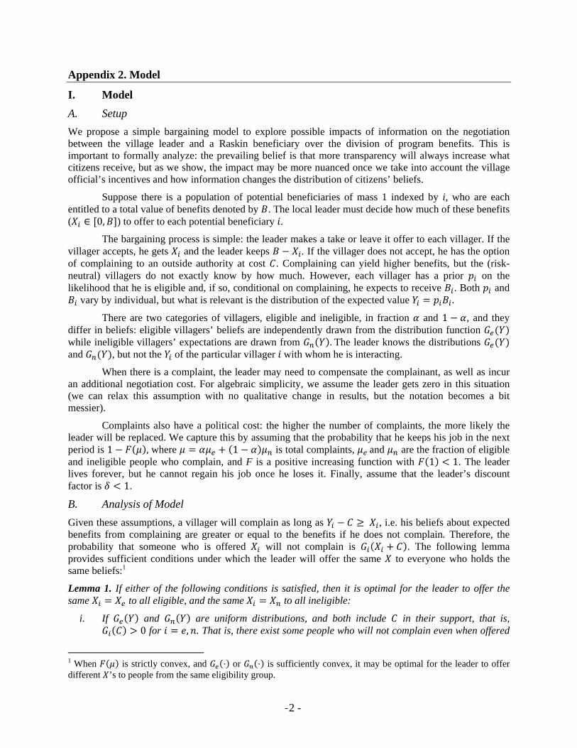
∈ 0,1 . We always have that 0, 0 and 0. The benefit to eligible rises if absent the

intervention there are sufficiently many complaints. Specifically, 0 if and only if

1 .

The intuition is as follows: increasing increases the fraction of eligible households who complain, holding constant. This decreases the future value of being a leader, so the leader offers less to ineligibles, i.e. decreases and complaints increase. For eligibles, there are again two offsetting effects: there are fewer eligible people accepting the offer, which reduces the cost of sweetening the offer to them but the future value of being in office has declined, which will lead the official to reduce . Which of these effects dominates is theoretically ambiguous.

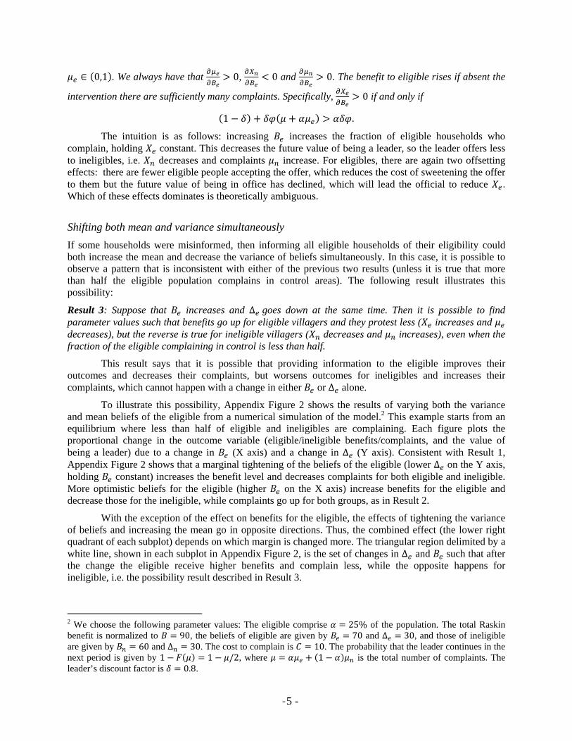
Shifting both mean and variance simultaneously

If some households were misinformed, then informing all eligible households of their eligibility could both increase the mean and decrease the variance of beliefs simultaneously. In this case, it is possible to observe a pattern that is inconsistent with either of the previous two results (unless it is true that more than half the eligible population complains in control areas). The following result illustrates this possibility:

Result 3: Suppose that increases and Δ goes down at the same time. Then it is possible to find parameter values such that benefits go up for eligible villagers and they protest less ( increases and decreases), but the reverse is true for ineligible villagers ( decreases and increases), even when the fraction of the eligible complaining in control is less than half.

This result says that it is possible that providing information to the eligible improves their outcomes and decreases their complaints, but worsens outcomes for ineligibles and increases their complaints, which cannot happen with a change in either or Δ alone.

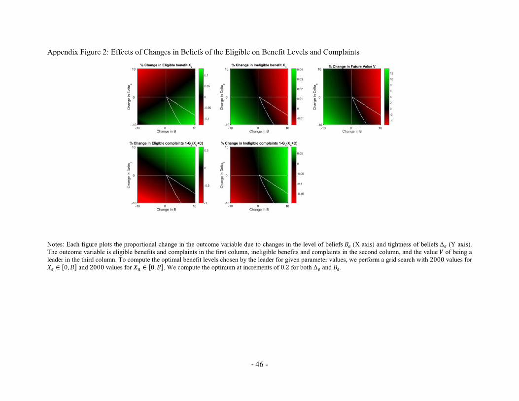
To illustrate this possibility, Appendix Figure 2 shows the results of varying both the variance and mean beliefs of the eligible from a numerical simulation of the model.2 This example starts from an equilibrium where less than half of eligible and ineligibles are complaining. Each figure plots the proportional change in the outcome variable (eligible/ineligible benefits/complaints, and the value of being a leader) due to a change in (X axis) and a change in Δ (Y axis). Consistent with Result 1, Appendix Figure 2 shows that a marginal tightening of the beliefs of the eligible (lower Δ on the Y axis, holding constant) increases the benefit level and decreases complaints for both eligible and ineligible. More optimistic beliefs for the eligible (higher on the X axis) increase benefits for the eligible and decrease those for the ineligible, while complaints go up for both groups, as in Result 2.

With the exception of the effect on benefits for the eligible, the effects of tightening the variance of beliefs and increasing the mean go in opposite directions. Thus, the combined effect (the lower right quadrant of each subplot) depends on which margin is changed more. The triangular region delimited by a white line, shown in each subplot in Appendix Figure 2, is the set of changes in Δ and such that after the change the eligible receive higher benefits and complain less, while the opposite happens for ineligible, i.e. the possibility result described in Result 3.

2 We choose the following parameter values: The eligible comprise 25% of the population. The total Raskin benefit is normalized to 90, the beliefs of eligible are given by 70 and Δ 30, and those of ineligible are given by 60 and Δ 30. The cost to complain is 10. The probability that the leader continues in the next period is given by 1 1 /2, where 1 is the total number of complaints. The leader’s discount factor is 0.8.

‐ 6 -

In short, the results suggest that the impacts of information are not, ex-ante, obvious – while they may improve outcomes, we cannot a priori rule out the perverse possibility that they may worsen them, if they decrease the future value of holding office for the local official making the decisions.

Appendix 3. Model Proofs

Lemma 1. If either of the following conditions is satisfied, then it is optimal for the leader to offer the same to all eligible, and the same to all ineligible:

i. If and are uniform distributions, and both include in their support, that is, 0 for , . That is, there exists some people who will not complain even when

offered zero. ii. If is weakly concave in total complaints 1 .

Proof. Assume without loss of generality that individuals are ordered such that those between 0 and are eligible, and the rest ineligible. The leader’s problem is to choose the measurable function : 0,1 → that maximizes the objective function:

1 1 1

For part (i), consider a candidate solution function . Consider the eligible first. Note that the leader would never offer a villager more than is required to ensure zero protest probability; that is, Δ for ∈ 0, . Together with the hypothesis 0, this implies that 1 is a linear function for in the support of for ∈ 0, . Note also that is a quadratic concave function for in the same support. Similar statements apply for the ineligible. It follows that the

leader can weakly increase his payoff by offering the eligible ∗ and offering the ineligible ∗ . Indeed, by offering these amounts the current period payoff increases, leaving the

level of complaints (and thus future payoffs) constant.

For part (ii), note that 1 ⋅ is convex. We first show that the leader can always do better by offering the same to all of the eligible households. Holding the allocation to ineligible constant, by Jensen’s inequality, the third term in the objective function satisfies:

1 1 1

1 1 Μ

Consider ∗∗ ∈ argmax 1 1 Μ , then the

objective function is upper bounded by:

‐ 7 -

∗∗ ∗∗

1 1 ∗∗ Μ

A similar argument now applies to the ineligible, hence there exists ∗∗ and the objective function is bounded above by:

∗∗ ∗∗ 1 ∗∗ ∗∗

1 1 ∗∗ 1 1 ∗∗

The above expression is the objective function when the leader offers ∗∗ to everyone in group , . Hence, we have shown that the leader can always do at least as good by offering the same to everyone in the same eligibility group. ∎


∈ 0,1 . Then 0, i.e. tightening eligible beliefs always (weakly) increases their allocation.

Starting from an equilibrium where 0.5, then 0, 0 and 0, i.e. when a minority of

eligible households complain absent the intervention, tightening eligible beliefs increases transfers to both eligible and ineligible, and both groups complain less. Otherwise, starting from an equilibrium

where 0.5, then is of ambiguous sign, and 0 and 0, i.e., transfers to eligible

increase, it is ambiguous what happens to eligible complaints, and the ineligible receive less and complain more.

Proof. Recall the first order conditions and the Bellman equation:

2 Δ (6)

2 Δ (7)

1 1 0 (3)

We now differentiate totally these equations with respect to Δ . From (6) and (7) we obtain:

Δ2

Δ1 (8)

Δ2

Δ (9)

Thus, the effects on and given by a change in the variance of eligible beliefs depends on what happens to the value from being a leader . For the Bellman equation (3), by the envelope theorem we can ignore the partial derivatives with respect to and . We obtain:

Δ Δ0

⇒ 1 1Δ

Δ Δ

0

‐ 8 -

⇒Δ 1 1 Δ

Using (6) and the definition of , and writing out , we obtain:

Δ2Δ

1 1 2Δ

⋅

1 1 Δ

We now show that . If 0.5 then and 0. Consider the case when

0.5. Given that we start from an interior solution for complaints we have that 0

Δ , so it is sufficient to prove:

1 11

Note that 1 and 1 . We thus have

Δ 1 1 1 11 1

.

Together with (8) and (9), we conclude that 0 always, and 0 if and only if 0, which

happens if and only if the complaint rate for the eligible is initially above 50%.

Since ⋅ is unchanged, complaints by the ineligible move in opposite direction with . For eligible complaints, note that:

Δ Δ Δ12Δ Δ

.

When 0.5, we have 0 and 0, so 0. This means that following a tightening of

beliefs, complaints by the eligible go down. When 0.5, we have 0 but 0, so the overall

effect is ambiguous. The following numerical example shows that 0 is possible when the complaint

rate from eligible is sufficiently large in the absence of the intervention. Take 90, 10, 0.25, 130, 100, Δ Δ 50. When Δ increases by 10, the results are as follows.

Eligible Benefits

Ineligible Benefits

Eligible Complaints

Ineligible Complaints

Control (Δ ) 81.9 66.9 88.1% 73.1%

‐ 9 -

Treatment (Δ 10) 77.0 67.0 85.8% 73.0%

Difference -4.9 0.1 -2.3% -0.1%

In particular, note that complaints by eligible decrease. ∎

Result 2. Consider an equilibrium with an interior solution in terms of eligible complaints, that is

∈ 0,1 . We always have that 0, 0 and 0. The benefit to eligible rises if absent the

intervention there are sufficiently many complaints. Specifically, 0 if and only if

1 .

Proof. Differentiating the first order conditions with respect to we obtain:

2 1 (10)

2 (11)

From the Bellman equation we obtain:

0

⇒ 1 1 0

⇒1 1

Using (6) and the definition of , and writing out , we obtain:

2Δ

1 11

2Δ

1 10.

From (11) we conclude that 0, and given that ⋅ does not depend on we also have 0.

Eligible complaints always increase. Indeed, using the definition of we obtain:

1

The last equality applies (10). If 0 then 1 0. If 0 then 0 (recall

0). In either case, we conclude that eligible complaints increase.

‐ 10 -

From (10), the sign of the effect on the eligible is given by:

2 0 ⇔ 1

⇔ 1 1 1 ⇔ 1 .

This condition will fail when the leader is patient ( is large), is high, the eligible fraction is high, and the number of complaints is low. ∎

The results in the paper examined changes in information for eligible. The following states the result for changes for ineligibles, and considers as well changes in costs of complains:

Result 4. Starting from an equilibrium where 0.5, so a majority of ineligible households were not

complaining, we have 0, 0 and 0, 0. That is, changing ineligibles’ information

by raising their mean belief, by making them more precise, or both, increases benefits for the eligible and reduces their complaints.

Reducing the cost of complaining, always increases complaints for both groups. The effect on benefits

depends on the level of total complaints. If , then reducing reduces benefits for both

groups; if is above this threshold, reducing increases benefits for both groups.

Proof. For the first part, we apply Results 1 and 2, switching eligible and ineligible.

For the second part, differentiating the first order conditions with respect to we get:

2 1 (12)

2 1 (13)

From the Bellman equation we obtain:

0

⇒ 1 1 1 1

12Δ

112Δ

1 1

⇒1

1 1

From (12) and (13), the sign of and the sign of are determined by the sign of . Simple

algebra shows that this is positive if and only if . ∎

‐ 11 -

Appendix 4. Simulating the Model

In this Appendix, we explore the implications of the model numerically. We choose the following parameter values. The eligible comprise 25% of the population. The total Raskin benefit is normalized to 90, and the beliefs of eligible are given by 70 and Δ 30, and those of ineligible are given by 60 and Δ 30. The cost to complain is 10. The probability that the leader continues in the next period is given by 1 /2, where 1 is the total number of complaints. The leader’s discount factor is 0.8.

The optimal choice by the leader, under these parameter values, is to choose ∗ 71.3 and ∗ 66.3. It then follows that 31 percent of the eligible and 23 percent of the ineligible households

complain.

Appendix Figure 2 shows the results of varying the variance and level of beliefs of the eligible. Each subfigure plots the proportional change in the outcome variable (eligible/ineligible benefits/complaints, and the value of being a leader) due to a change in (X axis) and a change in Δ (Y axis). Consistent with Result 1, Appendix Figure 2 shows that a marginal tightening of the beliefs of the eligible (lower Δ on the Y axis) increases the benefit level and decreases complaints for both eligible and ineligible. In addition, more optimistic beliefs of the eligible (higher on the X axis) increase benefits for the eligible and decrease those for the ineligible, while complaints go up for both groups, which is consistent with Result 2.

With the exception of eligible benefits, the effects of tightening the beliefs and making them more optimistic go in opposite directions. Thus, the combined effect (the lower right quadrant of each subfigure) depends on which margin is changed more. In the case of benefits for and complaints by the ineligible, the combined effect is roughly linear in the two individual effects, with equal strengths. In the case of complaints by the eligible, the combined effect if roughly linear, with the change in Δ having a stronger effect.

We now compute numerically the set of parameter values for which the model predictions are consistent with what we find empirically. Assume that the baseline parameters chosen above correspond to the control group, namely Δ Δ 30 and 70, and the corresponding parameter in the treatment group are denoted Δ and . The region delimited by a white line, shown in each subplot in Appendix Figure 2, is the set of changes Δ Δ , such that in the treatment group the eligible receive higher benefits and complain less than in the control group, while the opposite happens for ineligible.

‐ 12 -

Appendix 5. Modelling the Bottom Decile Treatment

In this section we adapt the model to cover three eligibility groups, in order to consider theoretically the impact of providing only the bottom decile with cards.

Assume that the village leader can distinguish between two groups of the eligible beneficiaries: the bottom decile poorest eligible, and the rest of the eligible. In total, the leader deals the three groups: bottom decile eligible, other eligible, and ineligible, respectively denoted 1, 2 and . We extend the notation in the natural way; for example, the allocations to the three groups are denotes by , and

, respectively. Denote the shares of the three groups in the population by , and , which satisfy 1. We assume the re-election probability is given by . Lemma 1 continues to apply with the obvious modifications, and it implies that the leader offers the same to everyone in the same group.

The objective function of the village leader is now:

max, , 1 1 1 1

We focus on the policy experiment of giving out Raskin cards to eligible groups. There are two treatments: the “bottom decile” treatment provides cards to the bottom decile eligible ( 1) group only, while the “all eligible” treatment provides cards to all eligible, that is both groups 1 and 2.

Providing information may affect the beliefs of the two eligible groups by raising their mean belief, by making them more precise, or a combination of these effects. Moreover, it is possible that the two groups have baseline beliefs that are different, and it is possible that the treatment affects these beliefs differently. We assume that the beliefs of groups that do not receive information are not affected; substantively, this means that the beliefs of the 2 do not change under the “bottom decile” treatment, and the beliefs of ineligible are not affected by either treatment.

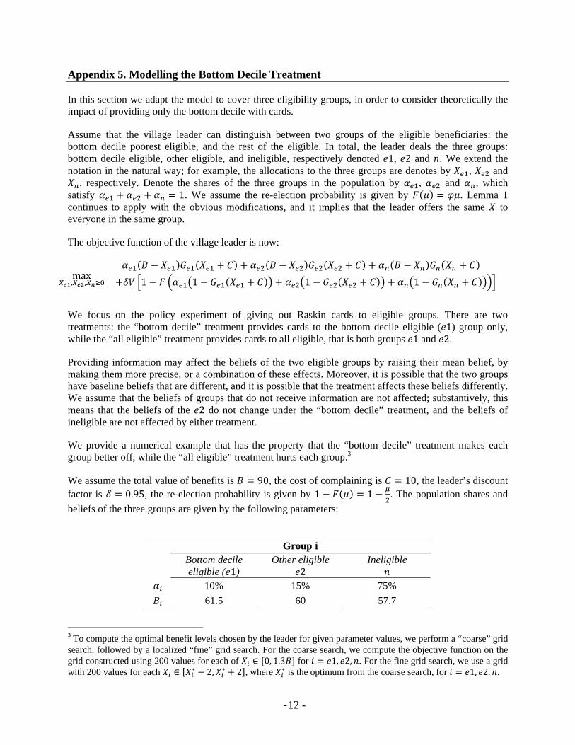
We provide a numerical example that has the property that the “bottom decile” treatment makes each group better off, while the “all eligible” treatment hurts each group.3

We assume the total value of benefits is 90, the cost of complaining is 10, the leader’s discount factor is 0.95, the re-election probability is given by 1 1 . The population shares and

beliefs of the three groups are given by the following parameters:

Group

Bottom decile eligible ( 1)

Other eligible 2

Ineligible

10% 15% 75%

61.5 60 57.7

3 To compute the optimal benefit levels chosen by the leader for given parameter values, we perform a “coarse” grid search, followed by a localized “fine” grid search. For the coarse search, we compute the objective function on the grid constructed using 200 values for each of ∈ 0, 1.3 for 1, 2, . For the fine grid search, we use a grid with 200 values for each ∈ ∗ 2, ∗ 2 , where ∗ is the optimum from the coarse search, for 1, 2, .

‐ 13 -

Δ 35 35 35 With these parameters, the leader optimally offers 84.5, 83.7 and 82.6 to the three groups. We assume that information increases the mean and decreases the spread of beliefs of the bottom decile eligible ( 1) group. For the other eligible ( 2) group, we assume information increases their mean belief. The specific parameter values are listed in the following table.

Beliefs Benefits Complaints

Δ

Control (values) 61.5 35 60 84.53 83.77 82.63 2.82% 1.75% 0.10%

“All eligible” treatment (changes)

1 1.3 4 1.00 0.15 2.16 1.15% 5.93% 3.09%

“Bottom decile” treatment (changes)

1 1.3 0 1.26 0.13 0.07

2.22% 0.17% 0.10%

The simulation results show that in the “all eligible” treatment the leader decreases the allocation to each of the three groups, and the number of complaints from each group goes up. However, providing information only to the bottom decile eligible leads to an increase in the allocation to each of the three groups, and complaints decrease across the board. The logic of this example is based on the intuition discussed in Results 1 and 2, which goes through in this modified form of the model. Specifically, an increase in the mean belief leads to a large decrease in the value to the leader; this occurs because at baseline there are only few complaints (Result 2). This effects makes the leader decrease the allocations to all three groups, including the other eligible, for whom beliefs increase. On its own, the change in beliefs to the bottom decile eligible has the opposite effect, mainly due the decrease in Δ , which tends to increase the value to the leader, again because of the low number of complaints at baseline (Result 1). When both groups have their beliefs affects in the “all eligible” treatment, the effect due to the other eligible dominates, and all groups lose out.

‐14‐

Appendix 6: Additional Appendix Tables List of Appendix Tables: Appendix Table 1A: Effect of Distributing Cards with Coupons on Card Receipt and Use Appendix Table 1B: Effect of Distributing Cards with Coupons on Subsidy Appendix Table 2: Summary Statistics for the Control Group Appendix Table 3: Randomization Check for Card Treatment Appendix Table 4: Randomization Check for Card Variations Appendix Table 5: Reduced Form Effect of Card Treatment on Card Receipt and Use,

Varying Controls Appendix Table 6: Reduced Form Effect of Card Treatment on Card Receipt and Use, No

Weights Appendix Table 7: Reduced Form Effect of Card Treatment on Card Receipt and Use,

Regional Heterogeneity Appendix Table 8: Reduced Form Effect of Card Treatment on Card Receipt and Use,

Corruption Heterogeneity Appendix Table 9: Reduced Form Effect of Card Treatment on Subsidy, Varying

Controls Appendix Table 10: Reduced Form Effect of Card Treatment on Subsidy, No Weights Appendix Table 11: Reduced Form Effect of Card Treatment on Subsidy, Regional

Heterogeneity Appendix Table 12: Reduced Form Effect of Card Treatment on Subsidy, Corruption

Heterogeneity Appendix Table 13: Relative Weight Estimates from Weighing Test Appendix Table 14: Reduced Form Effect of Card Treatment on Subsidy, Recall

Heterogeneity Appendix Table 15: Reduced Form Effect of Card Treatment on Subsidy, Conditional on

Purchase

‐15‐

Appendix Table 16: Effect of Card Treatment on Protests and Complaints, by Survey Round

Appendix Table 17: Effect of Printing Price on Cards on Card Receipt and Use Appendix Table 18: Effect of Printing Price on Cards on Subsidy, Conditional on Public

Information Appendix Table 19: Effect of Printing Price on Cards on Minimum and Maximum Prices

in the Village Appendix Table 20: Effect of Distributing Cards Only to the Bottom 10 Percent on Card

Receipt and Use Appendix Table 21: Effect of Only Distributing Cards to the Bottom 10 Percent on

Protests and Complaints Appendix Table 22: Effect of Public Information on Seeing the Eligibility List, Dropping

“Do Not Know” Answers Appendix Table 23: Effect of Public Information on Beliefs about Who Has Seen List, by

Eligibility Status Appendix Table 24: Effect of Public Information on Beneficiary Status Knowledge, by

Eligibility Status Appendix Table 25: Effect of Public Information on Protests and Complaints Appendix Table 26: Does Public Information Affect Subsidy Only Through Card

Receipt? Implied Instrumental Variables Estimation Appendix Table 27: Does Public Information Affect Subsidy Only Through Card

Receipt? Implied Instrumental Variables Estimation, First Stage and Reduced Form

List of Appendix Figures: Appendix Figure 1: Public Information Poster Appendix Figure 2: Effects of Changes in Beliefs of the Eligible on Benefit Levels and

Complaints Appendix Figure 3: Raskin Cards with and without price, Indonesian versions

‐16‐

Appendix Table 1A: Effect of Distributing Cards with Coupons on Card Receipt and Use

Eligible Households Ineligible Households Received

Card Used Card Used Coupon Received

Card Used Card Used Coupon (1) (2) (3) (4) (5) (6) Cards with Coupons 0.25*** 0.10*** 0.06*** 0.03* 0.03* 0.01 (0.03) (0.03) (0.01) (0.02) (0.02) (0.01) Cards without Coupons 0.26*** 0.10*** -0.00 0.03* 0.05*** -0.00 (0.03) (0.03) (0.01) (0.02) (0.02) (0.01) Difference: Coupons – No Coupons -0.01 -0.00 0.07*** -0.00 -0.02 0.01* (0.03) (0.03) (0.02) (0.02) (0.02) (0.01) Observations 5,693 5,693 5,693 3,619 3,619 3,619 Control Group Mean 0.07 0.06 0.01 0.05 0.04 0.01 Note: This table provides the reduced form effect of belonging to the Coupons and No Coupons treatment groups on card outcomes and knowledge, by eligibility status, as compared to the control group. Each column in this table comes from a separate OLS regression of respective outcome on the two treatments, strata fixed effects, survey sample dummies, and a dummy for whether the village was also in the public information treatment. We also provide the difference in the two card treatments. Data are pooled from the first and second follow-up survey. Eligible households that did not receive a card under the bottom ten treatment are dropped from the sample and we re-weight the treatment groups by sub-district so that the ratio of all three income groups is the same. Standard errors are clustered by village. *** p<0.01, ** p<0.05, * p<0.1

‐17‐

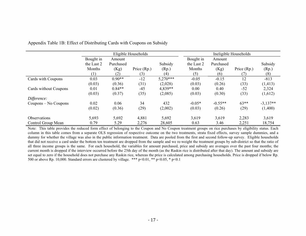
Appendix Table 1B: Effect of Distributing Cards with Coupons on Subsidy

Eligible Households Ineligible Households Bought in

the Last 2 Months

Amount Purchased

(Kg) Price (Rp.) Subsidy

(Rp.)

Bought in the Last 2 Months

Amount Purchased


(Rp.) (1) (2) (3) (4) (5) (6) (7) (8) Cards with Coupons 0.03 0.90** -12 5,270*** -0.05 -0.15 12 -813 (0.03) (0.36) (31) (2,028) (0.03) (0.26) (33) (1,413) Cards without Coupons 0.01 0.84** -45 4,839** 0.00 0.40 -52 2,324 (0.03) (0.37) (35) (2,085) (0.03) (0.30) (33) (1,612) Difference: Coupons – No Coupons 0.02 0.06 34 432 -0.05* -0.55** 63** -3,137** (0.02) (0.36) (29) (2,002) (0.03) (0.26) (29) (1,400) Observations 5,693 5,692 4,881 5,692 3,619 3,619 2,283 3,619 Control Group Mean 0.79 5.29 2,276 28,605 0.63 3.46 2,251 18,754 Note: This table provides the reduced form effect of belonging to the Coupon and No Coupon treatment groups on rice purchases by eligibility status. Each column in this table comes from a separate OLS regression of respective outcome on the two treatments, strata fixed effects, survey sample dummies, and a dummy for whether the village was also in the public information treatment. Data are pooled from the first and second follow-up survey. Eligible households that did not receive a card under the bottom ten treatment are dropped from the sample and we re-weight the treatment groups by sub-district so that the ratio of all three income groups is the same. For each household, the variables for amount purchased, price and subsidy are averages over the past four months; the current month is dropped if the interview occurred before the 25th day of the month (as the Raskin rice is distributed after that day). The amount and subsidy are set equal to zero if the household does not purchase any Raskin rice, whereas the price is calculated among purchasing households. Price is dropped if below Rp. 500 or above Rp. 10,000. Standard errors are clustered by village. *** p<0.01, ** p<0.05, * p<0.1

‐18 -

Appendix Table 2: Summary Statistics for the Control Group

Eligible Households Ineligible Households Observations Mean Std. Dev Observations Mean Std. Dev

(1) (2) (3) (4) (5) (6) Panel A: Card Receipt and Use

Received Card 2,275 0.07 0.25 1,207 0.05 0.22 Used Card 2,275 0.06 0.24 1,207 0.04 0.20 Knows Own Status 2,275 0.30 0.46 1,207 0.36 0.48

Panel B: Subsidy Bought in the Last 2 Months 2,275 0.79 0.40 1,207 0.63 0.48 Amount Purchased (Kg) 2,274 5.29 4.28 1,207 3.46 3.78 Price (Rp.) 1,923 2,276 461 813 2,251 461 Subsidy (Rp.) 2,274 28,605 23,653 1,207 18,754 20,609 Note: This table provides summary statistics for key outcome variables for the control group, by official eligibility status. The data are pooled from both the first and second follow-up survey. Price is dropped if below Rp. 500 or above Rp. 10,000.

‐19 -

Appendix Table 3: Randomization Check for Card Treatment

Means

Difference Between Treatment and

Control

N Control Treatment

No Controls

Stratum Fixed

Effects (1) (2) (3) (4) (5) Log consumption 5718 13.11 13.11 0.00 -0.00 (0.02) (0.02) PMT Score 5720 12.79 12.79 0.00 -0.00 (0.02) (0.02) Household Head Years of Education 5693 7.14 7.28 0.14 0.15 (0.18) (0.13) RT Head Years of Education 570 7.95 8.34 0.39 0.44 (0.31) (0.30) Village Distance to Kecamatan 572 6.48 7.27 0.79 0.25 (1.16) (1.06) Percentage of agriculture households 572 0.07 0.07 -0.01 -0.00 in RT (0.01) (0.01) Log Number of Households in RT 572 4.20 4.28 0.08* 0.09* (0.04) (0.04) Number of Primary Schools per 1,000 572 2.74 2.62 -0.12 -0.10 Households (0.12) (0.12) Log village size 572 4.02 3.95 -0.07 -0.08 (0.14) (0.07) Number of Religious buildings per 572 4.88 4.75 -0.12 -0.00 1,000 Households (0.32) (0.24) Joint test Chi square 7.84 14.23 Joint test P-value 0.64 0.16 Note: This table provides a check on the randomization for the main card treatment. The data come from the baseline survey. Columns 2 and 3 report the variable mean in the control and treatment groups, respectively. We then provide the difference in means with no controls (Column 4) and with strata fixed effects (Column 5). Joint significance Chi square tests across the multiple outcomes are reported. Standard errors are clustered by village. *** p<0.01, ** p<0.05, * p<0.1

‐20 -

Appendix Table 4: Randomization Check for Card Variations

N

Public – Standard

Information Cards to all - Bottom 10

Price - No Price

(1) (2) (3) (4) Log consumption 3779 0.01 -0.02 -0.01

(0.02) (0.02) (0.02) PMT Score 3780 0.01 0.01 -0.01

(0.02) (0.02) (0.02) Household Head Years of 3765 -0.20 -0.04 -0.01 Education (0.18) (0.15) (0.18) RT Head Years of Education 376 -0.38 0.53 0.09

(0.36) (0.41) (0.36) Village Distance to Kecamatan 378 -3.49* 2.06 2.70

(1.93) (2.46) (1.90) Percentage of agriculture 378 -0.01 0.00 -0.00 households in RT (0.01) (0.01) (0.01) Log Number of Households in 378 0.01 -0.06 0.02 RT (0.05) (0.06) (0.05) Number of Primary Schools 378 -0.02 0.10 0.16 per 1,000 Households (0.14) (0.14) (0.14) Log village size 378 -0.14 -0.09 -0.13

(0.11) (0.08) (0.11) Number of Religious buildings per 1,000 Households

378 -0.12 -0.23 0.68** (0.29) (0.27) (0.29)

Joint test Chi square 11.51 13.20 13.06 Joint test P-value 0.32 0.21 0.22 Note: This table provides a check on the randomization for card variations. The data come from the baseline survey. All of the differences presented are conditional on strata fixed effects. In the last two rows, we additionally report the joint significance Chi square tests across the multiple outcomes in each column. Standard errors are clustered by village. *** p<0.01, ** p<0.05, * p<0.1

‐21 -

‐22 -

Appendix Table 5: Reduced Form Effect of Card Treatment on Card Receipt and Use, Varying Controls

Eligible Households Ineligible Households

Received Card Used Card Knows own

status Received Card Used Card Knows own

status (1) (2) (3) (4) (5) (6)

Panel A: No Controls Card Treatment 0.28*** 0.14*** 0.09*** 0.03** 0.04*** 0.05* (0.02) (0.02) (0.02) (0.01) (0.01) (0.02)

Panel B: Adding Month Fixed Effects to Table 1 specification Card Treatment 0.30*** 0.15*** 0.09*** 0.03** 0.04*** 0.05**

(0.02) (0.02) (0.02) (0.01) (0.01) (0.02) Panel C: Adding Additional Baseline Controls to Table 1 specification

Card Treatment Controls and Additional Controls

0.30*** 0.15*** 0.09*** 0.03** 0.04*** 0.05** (0.02) (0.02) (0.02) (0.01) (0.01) (0.02)

Observations 5,693 5,693 5,691 3,619 3,619 3,619 Control Group Mean 0.07 0.06 0.30 0.05 0.04 0.36 Note: This table replicates Table 1, but with varying sets of controls. In Panel A, we omit all control variables. In Panel B, we add month fixed effects to the specification in Table 1, while we additionally include the 10 baseline variables from Appendix Table 3 in Panel C. Standard errors are clustered by village. *** p<0.01, ** p<0.05, * p<0.1

‐23 -

Appendix Table 6: Reduced Form Effect of Card Treatment on Card Receipt and Use, No Weights


Received Card Used Card

Knows Own Status on

Official List Received

Card Used Card

Knows Own Status on

Official List (1) (2) (3) (4) (5) (6) Card Treatment 0.30*** 0.15*** 0.10*** 0.03*** 0.04*** 0.05*** (0.02) (0.02) (0.02) (0.01) (0.01) (0.02)

Observations 5,699 5,699 5,697 3,620 3,620 3,620 Control Group Mean 0.06 0.06 0.30 0.05 0.04 0.35 Note: This table replicates Table 1, except sample weights are not used. Standard errors are clustered by village. *** p<0.01, ** p<0.05, * p<0.1

‐24 -

Appendix Table 7: Reduced Form Effect of Card Treatment on Card Receipt and Use, Regional Heterogeneity


Card Used Card Knows own

status Received

Card Used Card Knows own

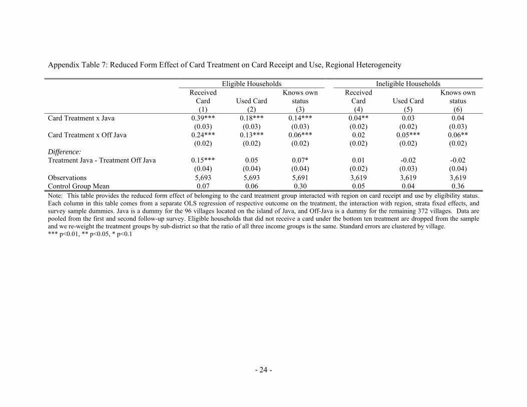
status (1) (2) (3) (4) (5) (6) Card Treatment x Java 0.39*** 0.18*** 0.14*** 0.04** 0.03 0.04 (0.03) (0.03) (0.03) (0.02) (0.02) (0.03) Card Treatment x Off Java 0.24*** 0.13*** 0.06*** 0.02 0.05*** 0.06** (0.02) (0.02) (0.02) (0.02) (0.02) (0.02) Difference: Treatment Java - Treatment Off Java 0.15*** 0.05 0.07* 0.01 -0.02 -0.02 (0.04) (0.04) (0.04) (0.02) (0.03) (0.04) Observations 5,693 5,693 5,691 3,619 3,619 3,619 Control Group Mean 0.07 0.06 0.30 0.05 0.04 0.36 Note: This table provides the reduced form effect of belonging to the card treatment group interacted with region on card receipt and use by eligibility status. Each column in this table comes from a separate OLS regression of respective outcome on the treatment, the interaction with region, strata fixed effects, and survey sample dummies. Java is a dummy for the 96 villages located on the island of Java, and Off-Java is a dummy for the remaining 372 villages. Data are pooled from the first and second follow-up survey. Eligible households that did not receive a card under the bottom ten treatment are dropped from the sample and we re-weight the treatment groups by sub-district so that the ratio of all three income groups is the same. Standard errors are clustered by village. *** p<0.01, ** p<0.05, * p<0.1

‐25 -

Appendix Table 8: Reduced Form Effect of Card Treatment on Card Receipt and Use, Corruption Heterogeneity


Received Card Used Card

Knows Own Status on

Official List Received

Card Used Card

Knows Own Status on

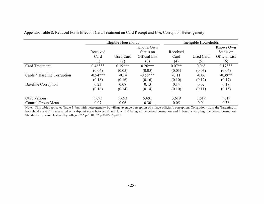
Official List (1) (2) (3) (4) (5) (6) Card Treatment 0.46*** 0.19*** 0.26*** 0.07** 0.06* 0.17*** (0.06) (0.05) (0.05) (0.03) (0.03) (0.06) Cards * Baseline Corruption -0.54*** -0.14 -0.58*** -0.11 -0.06 -0.39** (0.18) (0.16) (0.16) (0.10) (0.12) (0.17) Baseline Corruption 0.23 0.08 0.13 0.14 0.02 0.18 (0.16) (0.14) (0.14) (0.10) (0.11) (0.15) Observations 5,693 5,693 5,691 3,619 3,619 3,619 Control Group Mean 0.07 0.06 0.30 0.05 0.04 0.36 Note: This table replicates Table 1, but with heterogeneity by village average perception of village official’s corruption. Corruption (from the Targeting II household survey) is measured on a 4-point scale between 0 and 1, with 0 being no perceived corruption and 1 being a very high perceived corruption. Standard errors are clustered by village. *** p<0.01, ** p<0.05, * p<0.1

‐26 -

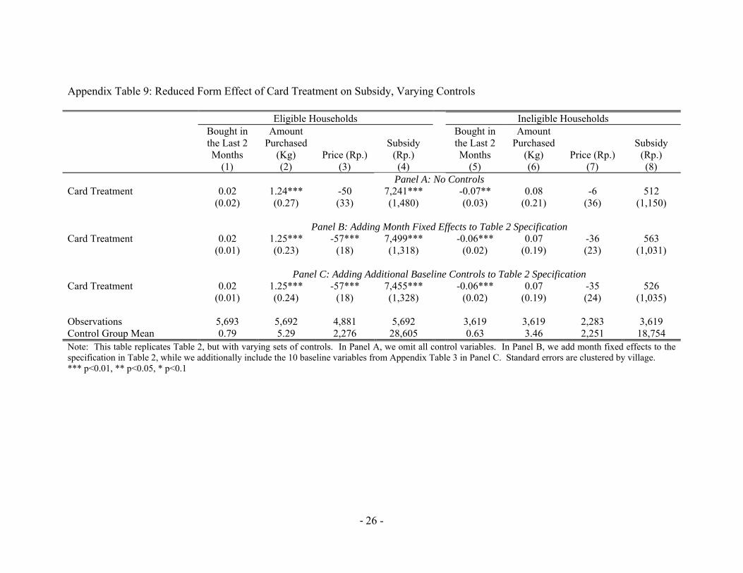
Appendix Table 9: Reduced Form Effect of Card Treatment on Subsidy, Varying Controls



Amount Purchased


(Rp.)


Amount Purchased


(Rp.) (1) (2) (3) (4) (5) (6) (7) (8) Panel A: No Controls Card Treatment 0.02 1.24*** -50 7,241*** -0.07** 0.08 -6 512 (0.02) (0.27) (33) (1,480) (0.03) (0.21) (36) (1,150) Panel B: Adding Month Fixed Effects to Table 2 Specification Card Treatment 0.02 1.25*** -57*** 7,499*** -0.06*** 0.07 -36 563 (0.01) (0.23) (18) (1,318) (0.02) (0.19) (23) (1,031) Panel C: Adding Additional Baseline Controls to Table 2 Specification Card Treatment 0.02 1.25*** -57*** 7,455*** -0.06*** 0.07 -35 526 (0.01) (0.24) (18) (1,328) (0.02) (0.19) (24) (1,035) Observations 5,693 5,692 4,881 5,692 3,619 3,619 2,283 3,619 Control Group Mean 0.79 5.29 2,276 28,605 0.63 3.46 2,251 18,754 Note: This table replicates Table 2, but with varying sets of controls. In Panel A, we omit all control variables. In Panel B, we add month fixed effects to the specification in Table 2, while we additionally include the 10 baseline variables from Appendix Table 3 in Panel C. Standard errors are clustered by village. *** p<0.01, ** p<0.05, * p<0.1

‐27 -

Appendix Table 10: Reduced Form Effect of Card Treatment on Subsidy, No Weights


the Last 2 Months

Amount Purchased

(Kg) Price (Rp.)

Subsidy (Rp.)


Amount Purchased

(Kg) Price (Rp.)

Subsidy (Rp.)

(1) (2) (3) (4) (5) (6) (7) (8) Card Treatment 0.02 1.27*** -52*** 7,649*** -0.05*** 0.09 -34 646 (0.01) (0.24) (17) (1,339) (0.02) (0.18) (24) (967)

Observations 5,699 5,698 4,881 5,698 3,620 3,620 2,284 3,620 Control Group Mean 0.79 5.29 2,263 28,706 0.63 3.43 2,272 18,438 Note: This table replicates Table 2, except sample weights are not used. Standard errors are clustered by village. *** p<0.01, ** p<0.05, * p<0.1

‐28 -

Appendix Table 11: Reduced Form Effect of Card Treatment on Subsidy, Regional Heterogeneity



Amount Purchased


(Rp.)


Amount Purchased


(Rp.) (1) (2) (3) (4) (5) (6) (7) (8) Card Treatment x Java 0.06** 1.77*** -58** 10,641*** -0.06 -0.08 -35 -355 (0.02) (0.38) (25) (2,307) (0.04) (0.22) (31) (1,300) Card Treatment x Off Java -0.00 0.94*** -56** 5,552*** -0.06** 0.16 -35 1,100 (0.02) (0.29) (24) (1,596) (0.02) (0.27) (34) (1,483) Difference: Treatment Java – Treatment 0.06* 0.83* -1 5,089* 0.00 -0.24 0 -1,455 Off Java (0.03) (0.48) (35) (2,806) (0.04) (0.35) (46) (1,972) Observations 5,693 5,692 4,881 5,692 3,619 3,619 2,283 3,619 Control Group Mean 0.79 5.29 2,276 28,605 0.63 3.46 2,251 18,754 Note: This table provides the reduced form effect of belonging to the card treatment group interacted with region on rice purchases and price by eligibility status. Each column in this table comes from a separate OLS regression of respective outcome on the treatment, the interaction with region, strata fixed effects, and survey sample dummies. Java is a dummy for the 96 villages located on the island of Java, and Off-Java is a dummy for the remaining 372 villages. Data are pooled from the first and second follow-up survey. Eligible households that did not receive a card under the bottom ten treatment are dropped from the sample and we re-weight the treatment groups by sub-district so that the ratio of all three income groups is the same. Standard errors are clustered by village. *** p<0.01, ** p<0.05, * p<0.1

‐29 -

Appendix Table 12: Reduced Form Effect of Card Treatment on Subsidy, Corruption Heterogeneity


the Last 2 Months

Amount Purchased

(Kg) Price (Rp.)

Subsidy (Rp.)


Amount Purchased

(Kg) Price (Rp.)

Subsidy (Rp.)

(1) (2) (3) (4) (5) (6) (7) (8) Card Treatment 0.09** 2.14*** -95* 12,939*** -0.05 0.02 -85 664 (0.04) (0.70) (49) (4,026) (0.06) (0.49) (76) (2,786) Cards * Baseline Corruption

-0.24** -2.91 114 -17,933

-0.03 0.14 150 -408

(0.12) (2.01) (142) (11,538) (0.16) (1.51) (221) (8,494) Baseline Corruption 0.03 2.04 -180 12,709 -0.03 -0.28 -213 826 (0.11) (1.83) (146) (10,209) (0.13) (1.50) (211) (8,411) Observations 5,693 5,692 4,881 5,692 3,619 3,619 2,283 3,619 Control Group Mean 0.79 5.29 2,276 28,605 0.63 3.46 2,251 18,754 Note: This table replicates Table 2, but with heterogeneity by village average perception of village official’s corruption. Corruption (from the Targeting II household survey) is measured on a 4-point scale between 0 and 1, with 0 being no perceived corruption and 1 being a very high perceived corruption. Standard errors are clustered by village. *** p<0.01, ** p<0.05, * p<0.1

‐30 -

Appendix Table 13: Relative Weight Estimates from Weighing Test

Weight Estimate (Respondent FE)

Weight Estimate (No FE)

(1) (2) Packet Weighing 6kg

1.56*** 1.56*** (0.33) (0.29)

Packet Weighing 7kg

3.97*** 3.97*** (0.50) (0.44)

Packet Weighing 8kg

4.75*** 4.75*** (0.75) (0.65)

Number of observations 72 72 Mean Weight Estimate for Packet Weighing 4kg

3.92 3.92

P-Values of Difference 6kg - 7kg 0.00 0.00 P-Values of Difference 6kg - 8kg 0.00 0.00 P-Values of Difference 7kg - 8kg 0.26 0.19 Note: This table provides the results of a weighing test in which eighteen eligible households in our sample guessed the weights of 4 packets of rice (in random order) that weighed 4, 6, 7, and 8kg. The table comes from an OLS regression of weight estimate on dummies for each packet. Column (1) includes respondent fixed effects, while Column (2) does not. Standard errors are clustered by respondent. *** p<0.01, ** p<0.05, * p<0.1

‐31 -

Appendix Table 14: Reduced Form Effect of Card Treatment on Subsidy, Recall Heterogeneity

Bought in Last 2

Months

Bought Last

Month

Average Amount

Purchased

Amount Purchased

Last Month Average

Price Price Last

Month Average Subsidy

Subsidy Last Month

(1) (2) (3) (4) (5) (6) (7) (8) Panel A: Eligible Households

Card Treatment 0.02 0.03* 1.25*** 1.43*** -57*** -67*** 7,455*** 8,465*** (0.01) (0.02) (0.24) (0.29) (18) (17) (1,328) (1,621)

Observations 5,693 5,690 5,692 5,689 4,881 4,278 5,692 5,689 Control Mean 0.79 0.73 5.29 5.88 2,276 2,276 28,605 31,505 Panel B: Ineligible Households Card Treatment -0.06*** -0.06*** 0.07 0.00 -35 -39 526 209

(0.02) (0.02) (0.19) (0.24) (24) (24) (1,035) (1,321) Observations 3,619 3,619 3,619 3,619 2,283 1,947 3,619 3,619 Control Mean 0.63 0.58 3.46 3.93 2,251 2,238 18,754 21,089 Note: Odd columns (1, 3, 5, 6, 7) replicate Table 2, while even columns (2, 4, 6, 8) restrict the sample to the past month’s Raskin purchase, rather than averaging over multiple months of Raskin. Standard errors are clustered by village. *** p<0.01, ** p<0.05, * p<0.1

‐32 -

Table 15: Reduced Form Effect of Card Treatment on Subsidy, Conditional on Purchase

Eligible Households Ineligible Households Amount

Purchased (Kg) Price (Rp.) Subsidy (Rp.)

Amount Purchased

(Kg) Price (Rp.) Subsidy (Rp.) (1) (2) (3) (4) (5) (6) Card Treatment 1.25*** -57*** 7,452*** 0.53** -35 3,181** (0.24) (18) (1,390) (0.23) (24) (1,309) Observations 4,885 4,881 4,885 2,286 2,283 2,286 Control Group Mean 6.20 2,276 33,502 5.19 2,251 28,118 Note: This table provides the reduced form effect of belonging to the card treatment group on rice purchases by eligibility status, conditional on buying subsidized rice. Each column in this table comes from a separate OLS regression of respective outcome on the treatment, strata fixed effects, and survey sample dummies. Data are pooled from the first and second follow-up surveys. Eligible households that did not receive a card under the bottom ten treatment are dropped from the sample and we re-weight the treatment groups by sub-district so that the ratio of all three income groups is the same. For each household, the variables for amount purchased, price and subsidy are averages over the past four months; the current month is dropped if the interview occurred before the 25th day of the month (as the Raskin rice is distributed after that day). The amount and subsidy are set equal to zero if the household does not purchase any Raskin rice, whereas the price is calculated among purchasing households. Price is dropped if below Rp. 500 or above Rp. 10,000. Standard errors are clustered by village. *** p<0.01, ** p<0.05, * p<0.1

‐33 -

Appendix Table 16: Effect of Card Treatment on Protests and Complaints, by Survey Round

Indicator for whether village leaders reports any…

“Protests”

“Complaints” by those who receive

rice

“Complaints” by those who do not

receive rice “Complaints” about list of beneficiaries

“Complaints” about distribution process

(1) (2) (3) (4) (5) Panel A: Survey Round 1 (Approximately 2 months)

Card Treatment 0.09*** -0.06 0.10** 0.14*** -0.04 (0.03) (0.05) (0.04) (0.04) (0.04) Number of observations 572 572 572 572 572 Control Group Mean 0.09 0.39 0.19 0.16 0.29 Panel B: Survey Round 2 (Approximately 8 months) Card Treatment 0.05 -0.13*** 0.05 0.02 -0.09* (0.03) (0.05) (0.04) (0.04) (0.05) Number of observations 571 572 572 572 572 Control Group Mean 0.13 0.46 0.26 0.20 0.53 P-Value of Difference 1 - 2 0.39 0.28 0.30 0.02 0.48 Note: This table provides the reduced form effect of belonging to the card treatment group on village leaders’ reports of protests or complaints related to the Raskin program in the 12 months preceding the survey, separated by survey round. Each column in this table comes from a separate OLS regression of respective outcome on the treatment and strata fixed effects. Standard errors are clustered by village. *** p<0.01, ** p<0.05, * p<0.1

‐34 -

Appendix Table 17: Effect of Printing Price on Cards on Card Receipt and Use


Card Used Card Received

Card Used Card (1) (2) (3) (4) Cards with Printed Price 0.25*** 0.12*** 0.03* 0.05** (0.03) (0.03) (0.02) (0.02) Cards without Price 0.25*** 0.07*** 0.03** 0.03* (0.03) (0.03) (0.02) (0.02) Difference: Price - No Price 0.01 0.04 0.00 0.02 (0.03) (0.03) (0.02) (0.02) Observations 5,688 5,688 3,615 3,615 Control Group Mean 0.07 0.06 0.05 0.04 Note: This table provides the reduced form effect of belonging to the Price and No Price treatment groups on card outcomes and knowledge, by eligibility status, as compared to the control group. Data are pooled from the first and second follow-up survey. Eligible households that did not receive a card under the bottom ten treatment are dropped from the sample and we re-weight the treatment groups by sub-district so that the ratio of all three income groups is the same. Each column in this table comes from a separate OLS regression of respective outcome on the two treatments, strata fixed effects, survey sample dummies, and a dummy for whether the village was also in the public information treatment. Standard errors are clustered by village. *** p<0.01, ** p<0.05, * p<0.1

‐35 -

Appendix Table 18: Effect of Printing Price on Cards on Subsidy, Conditional on Public Information



Amount Purchased


(Rp.)


Amount Purchased


(Rp.) (1) (2) (3) (4) (5) (6) (7) (8) Cards with Printed Price x -0.01 0.76 -66 4,650 -0.08* -0.39 -49 -2,145 Public Information (0.03) (0.51) (44) (2,917) (0.05) (0.37) (42) (2,022) Cards without Price x -0.01 0.83* -30 4,825* -0.04 0.33 -28 1,961 Public Information (0.03) (0.47) (34) (2,609) (0.04) (0.37) (38) (1,959) Cards with Printed Price 0.03 1.19*** -40 6,845*** -0.02 0.28 -39 1,813 (0.03) (0.40) (41) (2,265) (0.04) (0.32) (37) (1,739) Cards without Printed Price 0.02 0.53 -15 3,155 -0.04 -0.05 13 -458 (0.03) (0.38) (29) (2,113) (0.04) (0.31) (33) (1,662) Difference: Price and Public – Price and -0.04 -0.43 -26 -2,194 -0.06 -0.67 -10 -3,959 Standard (0.06) (0.82) (79) (4,682) (0.07) (0.62) (71) (3,412) Observations 5,688 5,687 4,877 5,687 3,615 3,615 2,281 3,615 Control Group Mean 0.79 5.29 2,276 28,605 0.63 3.46 2,251 18,754 Note: This table provides the reduced form effect of belonging to the Price and No Price treatment groups on rice purchases by eligibility status, conditional on public information. Each column in this table comes from a separate OLS regression of respective outcome on the two treatments, interactions of the two treatments with public information, strata fixed effects, and survey sample dummies. We also provide the difference in the two card treatments. Data are pooled from the first and second follow-up survey. Eligible households that did not receive a card under the bottom ten treatment are dropped from the sample and we re-weight the treatment groups by sub-district so that the ratio of all three income groups is the same. For each household, the variables for amount purchased, price and subsidy are averages over the past four months; the current month is dropped if the interview occurred before the 25th day of the month (as the Raskin rice is distributed after that day). The amount and subsidy are set equal to zero if the household does not purchase any Raskin rice, whereas the price is calculated among purchasing households. Standard errors are clustered by village. *** p<0.01, ** p<0.05, * p<0.1

‐36 -

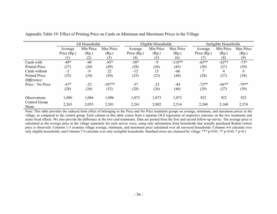
Appendix Table 19: Effect of Printing Price on Cards on Minimum and Maximum Prices in the Village

All Households Eligible Households Ineligible Households

Average

Price (Rp.) Min Price

(Rp.) Max Price

(Rp.) Average


(Rp.) Max Price

(Rp.) Average


(Rp.) Max Price

(Rp.) (1) (2) (3) (4) (5) (6) (7) (8) (9) Cards with -49* -40 -85* -50* -9 -110** -65** -62** -73* Printed Price (27) (26) (49) (28) (26) (45) (30) (27) (39) Cards without -2 -9 22 -12 15 -66 7 4 6 Printed Price (25) (24) (50) (25) (23) (44) (28) (27) (38) Difference: Price – No Price -47* -32 -107** -37 -23 -44 -72** -66** -79** (28) (26) (52) (28) (26) (46) (29) (27) (39) Observations 1,096 1,096 1,096 1,073 1,073 1,073 922 922 922 Control Group Mean

2,263 2,055 2,581

2,261 2,082 2,514

2,260 2,160 2,374

Note: This table provides the reduced form effect of belonging to the Price and No Price treatment groups on average, minimum, and maximum prices in the village, as compared to the control group. Each column in this table comes from a separate OLS regression of respective outcome on the two treatments and strata fixed effects. We also provide the difference in the two card treatments. Data are pooled from the first and second follow-up survey. The average price is calculated as the average price in the village separately for each survey wave, using only information from households that actually purchased Raskin (where price is observed). Columns 1-3 examine village average, minimum, and maximum price calculated over all surveyed households; Columns 4-6 calculate over only eligible households; and Columns 7-9 calculate over only ineligible households. Standard errors are clustered by village. *** p<0.01, ** p<0.05, * p<0.1

‐37 -

Appendix Table 20: Effect of Distributing Cards Only to the Bottom 10 Percent on Card Receipt and Use

Bottom 10 Households Other Eligible Households Ineligible Households

Received Card

Used Card

Knows Own

Status Received

Card Used Card

Knows Own

Status Received

Card Used Card

Knows Own

Status (1) (2) (3) (4) (5) (6) (7) (8) (9) Card to Bottom 10 0.25*** 0.09*** 0.04 0.04 0.04 0.01 0.04** 0.04** -0.00 (0.03) (0.03) (0.03) (0.02) (0.03) (0.03) (0.02) (0.02) (0.03) Cards to All 0.26*** 0.12*** 0.04 0.27*** 0.16*** 0.09*** 0.05*** 0.06*** 0.03 (0.03) (0.03) (0.03) (0.03) (0.03) (0.03) (0.02) (0.02) (0.03) Difference: Bottom 10 – All -0.01 -0.04 -0.00 -0.23*** -0.13*** -0.08*** -0.01 -0.02 -0.03 (0.03) (0.03) (0.03) (0.02) (0.02) (0.03) (0.02) (0.02) (0.02) Observations 3,683 3,683 3,683 2,968 2,968 2,966 3,619 3,619 3,619 Control Group Mean 0.07 0.06 0.31 0.06 0.05 0.28 0.05 0.04 0.37 Note: This table provides the reduced form effect of belonging to the Bottom Ten and All Cards treatment groups on card outcomes and knowledge, by eligibility status, as compared to the control group. Each column in this table comes from a separate OLS regression of respective outcome on the two treatments, strata fixed effects, survey sample dummies, and a dummy for whether the village was also in the public information treatment. We also provide the difference in the two card treatments. Data are pooled from the first and second follow-up survey. Standard errors are clustered by village.*** p<0.01, ** p<0.05, * p<0.1

‐38 -

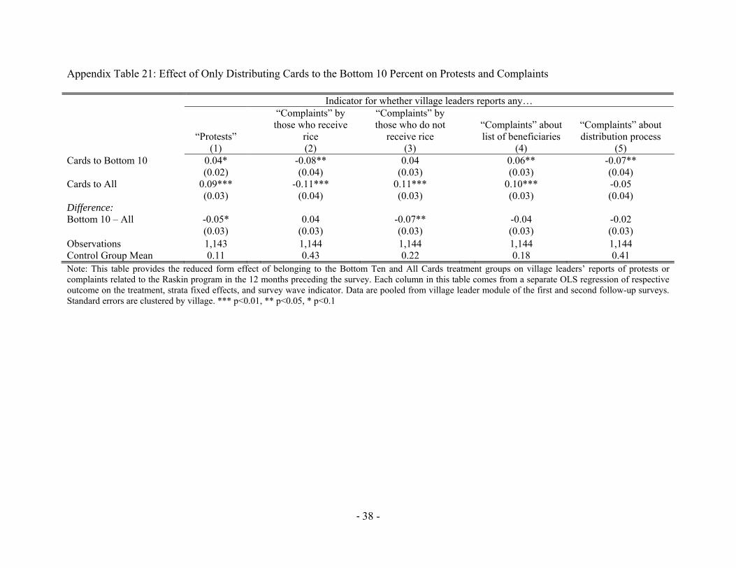
Appendix Table 21: Effect of Only Distributing Cards to the Bottom 10 Percent on Protests and Complaints


“Protests”

“Complaints” by those who receive

rice


receive rice “Complaints” about list of beneficiaries

“Complaints” about distribution process

(1) (2) (3) (4) (5) Cards to Bottom 10 0.04* -0.08** 0.04 0.06** -0.07**

(0.02) (0.04) (0.03) (0.03) (0.04) Cards to All

0.09*** -0.11*** 0.11*** 0.10*** -0.05 (0.03) (0.04) (0.03) (0.03) (0.04)

Difference: Bottom 10 – All -0.05* 0.04 -0.07** -0.04 -0.02

(0.03) (0.03) (0.03) (0.03) (0.03) Observations 1,143 1,144 1,144 1,144 1,144 Control Group Mean 0.11 0.43 0.22 0.18 0.41 Note: This table provides the reduced form effect of belonging to the Bottom Ten and All Cards treatment groups on village leaders’ reports of protests or complaints related to the Raskin program in the 12 months preceding the survey. Each column in this table comes from a separate OLS regression of respective outcome on the treatment, strata fixed effects, and survey wave indicator. Data are pooled from village leader module of the first and second follow-up surveys. Standard errors are clustered by village. *** p<0.01, ** p<0.05, * p<0.1

‐39 -

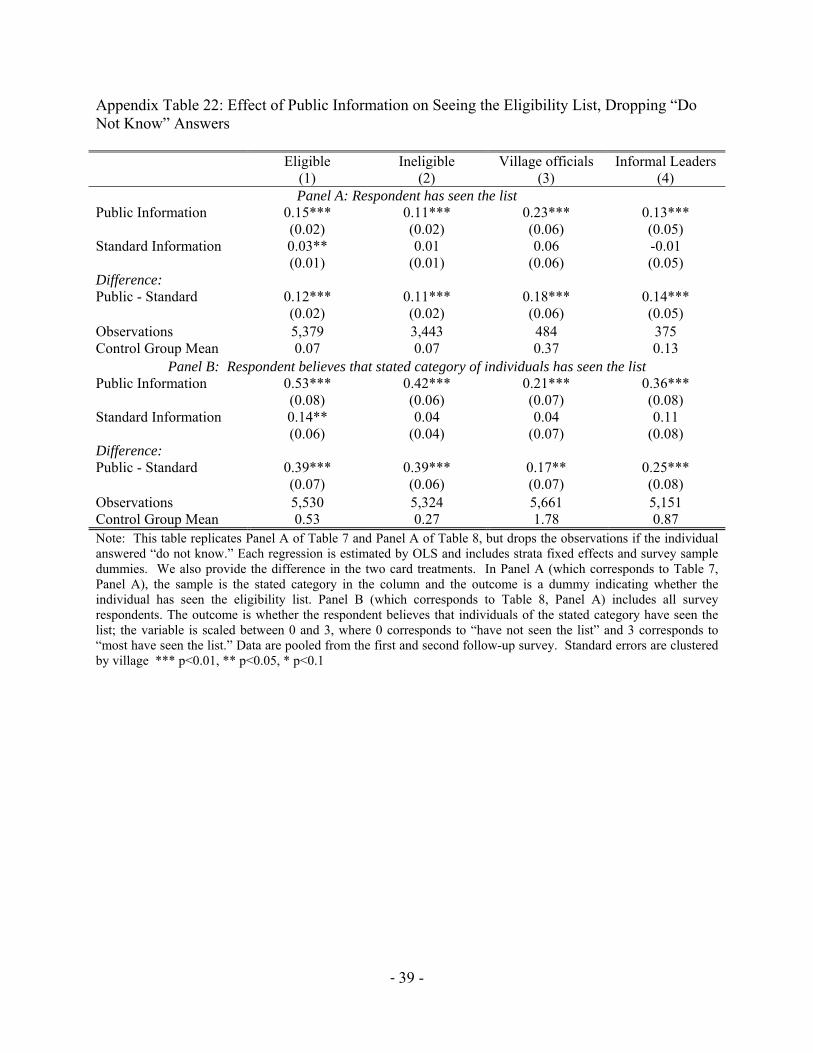
Appendix Table 22: Effect of Public Information on Seeing the Eligibility List, Dropping “Do Not Know” Answers

Eligible Ineligible Village officials Informal Leaders (1) (2) (3) (4)

Panel A: Respondent has seen the list Public Information 0.15*** 0.11*** 0.23*** 0.13*** (0.02) (0.02) (0.06) (0.05) Standard Information 0.03** 0.01 0.06 -0.01 (0.01) (0.01) (0.06) (0.05) Difference: Public - Standard 0.12*** 0.11*** 0.18*** 0.14*** (0.02) (0.02) (0.06) (0.05) Observations 5,379 3,443 484 375 Control Group Mean 0.07 0.07 0.37 0.13

Panel B: Respondent believes that stated category of individuals has seen the list Public Information 0.53*** 0.42*** 0.21*** 0.36*** (0.08) (0.06) (0.07) (0.08) Standard Information 0.14** 0.04 0.04 0.11 (0.06) (0.04) (0.07) (0.08) Difference: Public - Standard 0.39*** 0.39*** 0.17** 0.25*** (0.07) (0.06) (0.07) (0.08) Observations 5,530 5,324 5,661 5,151 Control Group Mean 0.53 0.27 1.78 0.87 Note: This table replicates Panel A of Table 7 and Panel A of Table 8, but drops the observations if the individual answered “do not know.” Each regression is estimated by OLS and includes strata fixed effects and survey sample dummies. We also provide the difference in the two card treatments. In Panel A (which corresponds to Table 7, Panel A), the sample is the stated category in the column and the outcome is a dummy indicating whether the individual has seen the eligibility list. Panel B (which corresponds to Table 8, Panel A) includes all survey respondents. The outcome is whether the respondent believes that individuals of the stated category have seen the list; the variable is scaled between 0 and 3, where 0 corresponds to “have not seen the list” and 3 corresponds to “most have seen the list.” Data are pooled from the first and second follow-up survey. Standard errors are clustered by village *** p<0.01, ** p<0.05, * p<0.1

‐40 -

Appendix Table 23: Effect of Public Information on Beliefs about Who Has Seen List, by Eligibility Status Eligible Ineligible Village Officials Informal Leaders (1) (2) (3) (4)

Panel A: Respondent is Eligible Public Information 0.38*** 0.29*** 0.25*** 0.27***

(0.05) (0.04) (0.06) (0.05) Standard Information 0.11** 0.04 0.04 0.08*

(0.04) (0.03) (0.06) (0.05) Difference:

Public - Standard 0.28*** 0.25*** 0.21*** 0.19*** (0.06) (0.04) (0.07) (0.06)

Number of observations 5,685 5,685 5,685 5,685 Control Group Mean 0.30 0.14 1.02 0.44

Panel B: Respondent is Ineligible Public Information 0.32*** 0.24*** 0.23*** 0.20***

(0.05) (0.04) (0.07) (0.06) Standard Information 0.02 -0.03 0.05 0.00

(0.04) (0.03) (0.07) (0.06) Difference:

Public - Standard 0.29*** 0.26*** 0.18*** 0.20*** (0.05) (0.04) (0.07) (0.06)

Number of observations 3,619 3,619 3,619 3,619 Control Group Mean 0.32 0.18 1.07 0.54 Note: This replicates Panel A of Table 8 by eligibility status of the respondent. Panel A includes only survey respondents eligible for Raskin, while Panel B includes only survey respondents ineligible to Raskin. The outcome is whether the individual believes that individuals in their village within each of the categories listed in the columns have seen the list of beneficiaries. The outcome varies from 0 to 3, where 0 corresponds to “have not seen the list” and 3 corresponds to “most have seen the list”; “Do not know” answers are coded as zero. Data are pooled from the first and second follow-up survey. Standard errors (in parentheses below coefficient) are clustered by village. *** p<0.01, ** p<0.05, * p<0.1

‐41 -

Appendix Table 24: Effect of Public Information on Beneficiary Status Knowledge, by Eligibility Status

Eligible Ineligible Village officials Informal Leaders (1) (2) (3) (4)

Panel A: Respondent is Eligible Public Information -0.01 0.01 -0.01 -0.03 (0.02) (0.02) (0.04) (0.04) Standard Information -0.00 0.04** 0.02 0.00 (0.02) (0.02) (0.04) (0.04) Difference: Public - Standard -0.00 -0.03* -0.03 -0.03 (0.02) (0.02) (0.04) (0.04) Observations 38,915 21,073 2,556 2,468 Control Group Mean 0.67 0.31 0.60 0.61

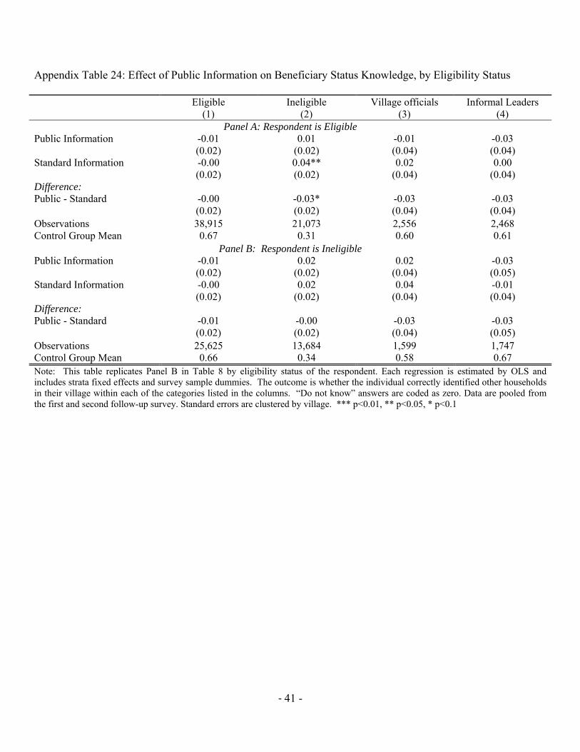
Panel B: Respondent is Ineligible Public Information -0.01 0.02 0.02 -0.03 (0.02) (0.02) (0.04) (0.05) Standard Information -0.00 0.02 0.04 -0.01 (0.02) (0.02) (0.04) (0.04) Difference: Public - Standard -0.01 -0.00 -0.03 -0.03 (0.02) (0.02) (0.04) (0.05) Observations 25,625 13,684 1,599 1,747 Control Group Mean 0.66 0.34 0.58 0.67 Note: This table replicates Panel B in Table 8 by eligibility status of the respondent. Each regression is estimated by OLS and includes strata fixed effects and survey sample dummies. The outcome is whether the individual correctly identified other households in their village within each of the categories listed in the columns. “Do not know” answers are coded as zero. Data are pooled from the first and second follow-up survey. Standard errors are clustered by village. *** p<0.01, ** p<0.05, * p<0.1

‐42 -

Appendix Table 25: Effect of Public Information on Protests and Complaints


“Protests”

“Complaints” by those who

receive rice


receive rice

“Complaints” about list of beneficiaries

“Complaints” about distribution

process (1) (2) (3) (4) (5) Public Information 0.10*** -0.10*** 0.10*** 0.12*** -0.09**

(0.03) (0.04) (0.03) (0.03) (0.04) Standard Information 0.03 -0.10*** 0.04 0.04 -0.07*

(0.02) (0.04) (0.03) (0.03) (0.04) Difference: Public - Standard 0.07** -0.00 0.06* 0.08** -0.02

(0.03) (0.03) (0.03) (0.03) (0.03) Observations 1,143 1,144 1,144 1,144 1,144 Control Group Mean 0.11 0.43 0.22 0.18 0.41 Note: This table provides the reduced form effect of belonging to the public information treatment group on village leaders’ reports of protests or complaints related to the Raskin program in the 12 months preceding the survey. Each column in this table comes from a separate OLS regression of respective outcome on the treatment, strata fixed effects, and survey wave indicator. Data are pooled from village leader module of the first and second follow-up surveys. Standard errors are clustered by village. *** p<0.01, ** p<0.05, * p<0.1

‐43 -

Appendix Table 26: Does Public Information Affect Subsidy Only Through Card Receipt? Implied Instrumental Variables Estimation

Public Information Standard Information (1) (2)

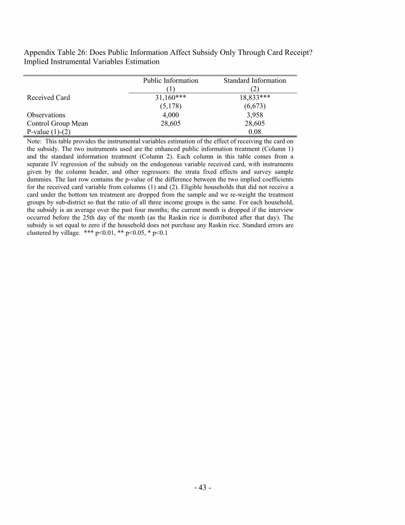
Received Card 31,160*** 18,833*** (5,178) (6,673) Observations 4,000 3,958 Control Group Mean 28,605 28,605 P-value (1)-(2) 0.08 Note: This table provides the instrumental variables estimation of the effect of receiving the card on the subsidy. The two instruments used are the enhanced public information treatment (Column 1) and the standard information treatment (Column 2). Each column in this table comes from a separate IV regression of the subsidy on the endogenous variable received card, with instruments given by the column header, and other regressors: the strata fixed effects and survey sample dummies. The last row contains the p-value of the difference between the two implied coefficients for the received card variable from columns (1) and (2). Eligible households that did not receive a card under the bottom ten treatment are dropped from the sample and we re-weight the treatment groups by sub-district so that the ratio of all three income groups is the same. For each household, the subsidy is an average over the past four months; the current month is dropped if the interview occurred before the 25th day of the month (as the Raskin rice is distributed after that day). The subsidy is set equal to zero if the household does not purchase any Raskin rice. Standard errors are clustered by village. *** p<0.01, ** p<0.05, * p<0.1

‐44 -

Appendix Table 27: Does Public Information Affect Subsidy Only Through Card Receipt? Implied Instrumental Variables Estimation, First Stage and Reduced Form

First Stage: Received Card Reduced Form: Subsidy (Rp.) Public

Information Standard

Information Public

Information Standard

Information (1) (2) (3) (4) Public Information 0.31*** 9,792*** (0.03) (1,689) Standard Information 0.25*** 4,759*** (0.03) (1,767) Observations 4,001 3,959 4,000 3,958 Control Group Mean 0.07 0.07 28,605 28,605 Note: This table provides the first stage and reduced form regressions for the IV estimates in Appendix Table 26. In the first two columns, the endogenous variable received card is regressed on the public and standard information treatments respectively. Column 1 omits households from villages randomly assigned to the standard information treatment, and Column 2 omits households from villages randomly assigned to the public information treatment. Columns 3 and 4 present the reduced form regression of subsidy received on public and standard information treatments respectively. Eligible households that did not receive a card under the bottom ten treatment are dropped from the sample and we re-weight the treatment groups by sub-district so that the ratio of all three income groups is the same. For each household, the subsidy is an average over the past four months; the current month is dropped if the interview occurred before the 25th day of the month (as the Raskin rice is distributed after that day). The subsidy is set equal to zero if the household does not purchase any Raskin rice. *** p<0.01, ** p<0.05, * p<0.1

‐45 -

Appendix Figure 1: Public Information Poster

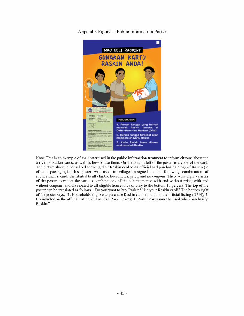
Note: This is an example of the poster used in the public information treatment to inform citizens about the arrival of Raskin cards, as well as how to use them. On the bottom left of the poster is a copy of the card. The picture shows a household showing their Raskin card to an official and purchasing a bag of Raskin (in official packaging). This poster was used in villages assigned to the following combination of subtreatments: cards distributed to all eligible households, price, and no coupons. There were eight variants of the poster to reflect the various combinations of the subtreatments: with and without price, with and without coupons, and distributed to all eligible households or only to the bottom 10 percent. The top of the poster can be translated as follows: “Do you want to buy Raskin? Use your Raskin card!” The bottom right of the poster says: “1. Households eligible to purchase Raskin can be found on the official listing (DPM); 2. Households on the official listing will receive Raskin cards; 3. Raskin cards must be used when purchasing Raskin.”

‐46 -

Appendix Figure 2: Effects of Changes in Beliefs of the Eligible on Benefit Levels and Complaints

Notes: Each figure plots the proportional change in the outcome variable due to changes in the level of beliefs (X axis) and tightness of beliefs Δ (Y axis). The outcome variable is eligible benefits and complaints in the first column, ineligible benefits and complaints in the second column, and the value of being a leader in the third column. To compute the optimal benefit levels chosen by the leader for given parameter values, we perform a grid search with 2000 values for

∈ 0, and 2000 values for ∈ 0, . We compute the optimum at increments of 0.2 for both Δ and .

‐47 -

Appendix Figure 3: Raskin Cards with and without price, Indonesian versions

TANGIBLE INFORMATION AND CITIZEN EMPOWERMENT...

Documents

Transcript of TANGIBLE INFORMATION AND CITIZEN EMPOWERMENT...