CFD analysis of sand particles erosion in a pipe bend Taline Muniz da Silveira Gomes

Department of Energy Technology, 4th semester MSc, 2021-06

Master’s Project

Copyright ⓍcA Aalborg University 2021

Energy Technology Aalborg University http://www.aau.dk

Title: CFD analysis of sand particles erosion in a pipe bend

Theme: Master Thesis in Process Engineering and Combustion Technology

Project Period: Feb-May 2021

Project Group: PECT10-2-21

Participant(s): Taline Muniz da Silveira Gomes

Supervisor: Matthias Mandø Company Supervisor: Anders Andreansen Page Numbers: 92

Date of Completion: May 28, 2021

The content of this report is freely available, but publication (with reference) may only be pursued due to

agreement with the author.

By accepting the request from the fellow student who uploads the study group’s project report in Digital Exam

System, you confirm that all group members have participated in the project work, and thereby all members are

collectively liable for the contents of the report. Furthermore, all group members confirm that the report

does not include plagiarism.

Contents

1. Introduction .................................................................................................................................................... 4

1.1 Sand particle erosion .................................................................................................................................... 5

1.2 Erosion models ............................................................................................................................................ 10

1.3 Flow regimes ............................................................................................................................................... 14

1.4 Empirical models ......................................................................................................................................... 17

2. Problem Statement ....................................................................................................................................... 22

3. CFD method .................................................................................................................................................. 23

3.1 CFD introduction ......................................................................................................................................... 23

3.2 Mesh independency analysis ...................................................................................................................... 24

3.3 Fluid flow model .......................................................................................................................................... 27

3.4 DPM sub-models ......................................................................................................................................... 28

4. Results .......................................................................................................................................................... 31

4.1 Case 1 – Gas and sand particles .................................................................................................................. 31

4.2 Case 2 – Water and sand particles .............................................................................................................. 35

4.3 Case 3 – Water and sand particles .............................................................................................................. 38

5. Discussion ..................................................................................................................................................... 42

6. Conclusion .................................................................................................................................................... 44

Bibliography .......................................................................................................................................................... 46

Appendix A – Tables .............................................................................................................................................. 48

Appendix B – CFD solution .................................................................................................................................... 50

1

Abstract

The presence of sand particles is a major concern in oil and gas pipelines, and it leads to damages and issues in the pipe, such as corrosion and erosion. Several studies have been developed to understand the parameters that affect the erosion in pipe as well as the models that can predict better results. Specially in a 90-degree pipe bend, due to the drastic change in the flow direction, erosion becomes a significant issue. A CFD model was used in this report to investigate the parameters that impact the erosion ate, such as pipe and particle diameters, fluid density and fluid velocity. Single-phase flows for air and water in the presence of sand particles were crated to simulate a turbulent flow and verify if the erosion rate would be similar to experimental data found in the literature review. Turbulence models available in ANSYS Fluent were utilized as well as DPM model engaging different sub-models to evaluate which cases could bring results similar to experimental work. Afterwards, two empirical models were taken into account, DNV GL RP O501 and API RP 14E, and the results were compared with CFD model and experimental results. The results obtained, showed that a CFD model can be used as a tool for predicting erosion rate, since it presented similar results to experiments, when the DPM sub-models for erosion, virtual mass force and stochastic collisions are considered in the simulation. Those cases considered forces acting in the particle and collisions of particle-to-particle and particle-to-wall that proved to be closer to an erosion rate obtained from a real case scenario. The API empirical model carries some limitations in the parameters used as inputs, however, the results calculated presented a similar result to experimental work with a tendency of underpredicting the erosion rate for water carrying sand particles. The DNV empirical model showed a tendency to overpredict the erosion rate for cases with water as the single-phase flow, and it is a safer case to be used for calculating the erosion in a 90-degree pipe bend. Comparing the case performed for gas and single-phase flow with two cases for water as the dispersed phase, the lowest erosion rate was found when water flow has particles of a smaller size, 150 𝜇m. Furthermore, in the presence of gas, that has a density of 1.225 kg/m3, the results obtained in CFD showed higher values than for water, with a density of 999.8 kg/m3. It can be concluded that when there is a considerable difference between the particle density and the fluid density, the erosion has a more significant impact in the pipe.

2

Preface

This report was written by Taline Muniz in the period that goes from February 1st, 2021 to May 28th, 2021. The project is part of a Master Thesis for the 4th semester of the Master’s Degree in Process Engineering and Combustion Technology at Aalborg University, Esbjerg, conducted in collaboration with Ramboll. The main objective of this project is to develop a Computational Fluid Dynamics (CFD) model to predict erosion in a 90-degree pipe bend. For this analysis, different erosion models using Euler-Lagrangian approach are investigated according to what is found in literature. The software ANSYS Fluent is used for this purpose. Additionally, a comparison with experiments found in literature will be evaluated, as well as with empirical models, to give an overview and an understanding of different equations from erosion prediction models. This project is carried under the supervision of the Associate Professor from Aalborg University, Matthias Mandø, and the Technical Manager from Ramboll, Anders Andreasen. Therefore, a special thanks for the guidance and supervision given throughout the project.

3

Nomenclature

Acronyms Description

API American Petroleum Institute

CFD Computational Fluid Dynamics

CRA Corrosion Resistant Alloy

DEM Discrete Element Method

DNV Det Norske Veritas

DPM Discrete Phase Model

MTBF Mean Time Before Failure

RANS Reynolds Averaged Navier-Stokes

Re Reynolds number

RP Recommend Practice

St Stokes number

4

1. Introduction In the oil and gas industry, sand transport is one of the major challenges for having a safe operation of the flow pipelines. The sand particles existing in the fluids extracted from the reservoir can cause financial and environmental problems. Mainly three issues often stand out in the operation: pressure drop, pipe blockage and erosion. This project will focus on sand particle erosion, which is one of the biggest concerns in single-phase and multiphase flows [1]. In the case of oil and gas being pumped out of the reservoirs accompanied by sand particles, it can have catastrophic consequences both offshore and onshore. Sand erosion can cause failure of equipment, leaks in pipelines resulting in environmental disasters and potential injury to personnel [2]. It can also change the surface geometry of the pipe, affecting its performance and shortening the Mean Time Before Failure (MTBF) [3]. 90-degree pipe bends are the biggest concern since that is when the erosion is more prevalent. As the sand particles flow into the bend, they abruptly change direction and collide with the pipe wall. A sequence of these impacts will cause erosion and decrease the lifespan of the pipe bends [1]. Alternatively, plugged tees are revealed as a good option instead of pipe bends, also called elbows, that show a significant erosion reduction when using a high particle loading [4]. Using this type of geometry creates an isolated area with high concentration of sand particles, facilitating the dynamics when a corrective action needs to take place. Hence, this increases the time before the pipe fails and improves the efficiency of the operation.

Therefore, any attempt to predict the damage caused by solid particles in a quantitative manner is a great interest for the oil and gas industry. Calculating the solid particle erosion rate is a helpful tool for helping design and preventing failures. In the last two decades, progress in the field of CFD have made possible to simulate erosion caused by sand particles in the flow with water, gas and oil. CFD is known to be the most useful and comprehensive approach for predicting vulnerable spots in piping systems and to estimate the erosion damage. The models used, can minimize such damages, optimize pipe geometry and flow conditions, as well as calculate the erosion rate using the particle impact velocity and angle of impact at the wall, to predict the MTBF of the bend pipe. However, the accuracy of the CFD models is very dependent on the sub-models that are included. Each sub-model is developed with certain assumptions about the physics that are being simulated. For predicting erosion models, usually there are two main categories: empirical and CFD-based. This report will focus on an empirical study comparing 2 models, Det Norske Veritas (DNV), and American Petroleum Institute Recommended Practice (API RP) 14E. For the CFD-based, DPM and several sub-models that will be described further, will be evaluated as well as their impact on the results found. Since there are several studies within this theme, the first step is to investigate the research reports that have being developed in the field of erosion modelling. The purpose is to find CFD models and sub-models, as well as the assumptions used that can be relevant for this report. A literature review within the empirical models is also made in order to understand the equations used to be replicated in this work.

5

1.1 Sand particle erosion

To better understand the research that has been made in prediction erosion rate, it is important to understand the erosion mechanism as well as the parameters involved for predicting solid particle erosion. When a particle impacts the wall surface, it scars the surface causing erosion that will depend on many parameters. The main ones are as such: particle shape, particle size, wall material, impact angle and particle-to-particle interaction [1] [2]. As mentioned earlier in this report, the wall material properties can be divided into two categories: ductile and brittle. Finnie [5] suggested that for ductile materials, the erosion is a result of micro-cutting. This mechanism happens when a particle hits the wall with a low impact and creates a crater. Several impacts will enlarge the crater and pile up material around it. The piled-up material is, then, removed by continuous particle impacts, creating the cutting mechanism shown in Fig. 01.

Fig. 01: Erosion in ductile materials. (a) before impact, (b) crater formed and material piled-up, (c)material removed from the surface [2]

For brittle materials, the erosion is caused by crack formation. When a particle collides at the wall surface, it creates both lateral and radial cracks. Further impacts will cause the cracks to grow. These cracks will eventually divide the surface into small pieces that can be removed by subsequent particle impacts (Fig. 02) [2].

Fig. 02: Erosion in brittle materials. (a) growth of cracks, (b) creation of lateral cracks, (c) eroded crater formed [2]

Many studies were proposed based on different erosion ratio equations which relate to the particle characteristics mentioned previously. Therefore, a more detailed explanation about those characteristics and their impact in the erosion rate will be presented. 1.1.1 Particle shape It has been observed that the shape of the particle has a significant impact in erosion. This is a factor introduced in many erosion ratio equations proposed by researchers, since the shape has a pronounced influence on erosion magnitude. For example, the sharpness of the particles has an influence in erosion [2]. Levy and Chik [33] studied two different shapes: sharp angular and spherical particles; and observed that the angular particles presented four times higher erosion when compared to the spherical ones.

6

1.1.2 Particle size The particle size is another factor taken into consideration when studying the erosion rate. The larger the particles, the larger is the kinetic energy. In Tilly’s study [9], he performed an experiment using particles of 0 to 200 𝜇m of diameter and flow velocities of 130, 240 and 300 m/s to evaluate erosion in a 90-degree elbow in a ductile material. He observed that for larger particles, bigger than approximately 100 𝜇m, the erosion ratio (mass eroded materials/mass of impact particles) is independent of particle sizes (Fig. 03).

Fig. 03: Erosion ratio versus particle size and particle impact velocity [9]

Gandhi and Borse [34] investigated the effect of sand particle size on erosion of cast iron in sand-water slurry using particles with diameters of 855 𝜇m, 505 𝜇m, 224 𝜇m and 112.5 𝜇m. The set-up was created placing two fixtures of cast iron separated at 180˚ apart in order to minimize the random impact angle and use the desired ones of 30˚ and 75˚. With a fluid velocity of 3.62 m/s, they observed a linear relation between sand size and erosion rate, shown in Fig. 04. The results were influenced by the fact that impact velocity of particles is not constant and changes with particle size when particles are in liquid flows.

Fig. 04: Effect of sand size on erosion rate flow velocity of 3.62 m/s [34]

Desale et al [35] studied the effect of particle size on aluminum alloy erosion for eight different sizes between 37.5 to 655 𝜇m, with a carrier fluid velocity of 3 m/s. Choosing two different impact angles, 30˚ and 90˚, they concluded that at a constant sand concentration, the larger the particle sizes, the higher is the erosion rate. The particle size shows to affect the particle impact velocity and the kinetic energy per impact (Fig. 05). For a slurry erosion, the mass loss can be influenced by other factors, such as particle impact velocity, fluid viscosity, particle concentration and particle-to-particle interactions.

7

Fig. 05: Effect of sand size on erosion rate [35]

Erosion of smaller particles can be influenced by particle-to-particle collisions, as the number of particle increases. In general, smaller sand particles can cause lower erosion rates, since they have smaller kinetic energy and impact force to erode a surface. However, they are more likely to be impacted by turbulence.

For a 90-degree pipe bend, a study compared different particle sizes, divided into small, medium and heavy sizes, with their particle trajectories. For small particles, with a low Stokes number, they will not be impacted by drag force to change their direction. However, for medium sized particles, there is a larger impact from drag force due to the increased in weight. Finally, for heavy particles, they will not be deflected by the fluid flow due to the higher momentum. After the elbow, they will hit the wall bouncing from one side to the other (Fig. 06) [42].

Fig. 06: Influence on flow paths of the different particle sizes in a 90-degree pipe bend. (a) small particles, (b) medium particles, (c) heavy

particles [42]

8

1.1.3 Wall material According to wall materials, the correlation between this factor and solid particle erosion is still not clear, despite experimental data results [2]. Finnie [5], in his study, proposed that the higher the hardness of the wall, the lower is the erosion. The opposite result was found by Levy and Hickey [37], when they observed that a material with high hardness results in higher erosion when compared with materials with lower hardness. Based on their observation, the material toughness could be a best indicator when analyzing the erosion rate. They have presented that toughness increases the erosion rate without reducing the ductility rate. The roughness of the wall also plays an important role when analyzing the erosion rate. A study on erosion in a 90-degree pipe bend showed that erosion rate for a rough wall is greater than for a smooth surface (Fig. 07) [41].

Fig. 07: Influence on erosion rate due to the roughness of the pipe wall surface [41]

1.1.4 Particle impact angle Studies were also developed observing the erosion rate in different particle impact angles. This effect is based on the wall material, ductile or brittle. For ductile materials, the lower impact angles present a higher erosion rate. This is due to more efficient formation and cutting mechanism at lower angles. On the other hand, for brittle materials, a higher erosion rate occurs with a normal particle impact (Fig. 08) [40].

Fig. 08: Erosion rate of different materials versus particle impact angle [40]

9

1.1.5 Particle-to-particle interaction The effect of particle-to-particle interaction has been observed by many researchers, since it has an important effect in the erosion rate. Duarte et al. [19] in 2015 investigated a mass loading effect on elbow erosion based on a four-way coupling simulation of multiphase flow carrying gas and sand. They worked with different amounts of mass loading, from 0.013 to 1.5 and concluded that inter-particle collision reduces the erosion rate. They also noticed, throughout experiments, that the higher number of particles, the lower is the erosion rate. The inter-particle collisions are responsible for the decreased in the erosion regions, due to more particle-to-particle collisions rather than particle-to-wall collisions. Brown et al. [38] and Deng et al. [39] observed the same results with high sand concentrations. When particles rebound from the wall, they hit other particles that move towards the wall and slow them down. This phenomenon is known as shielding. This goes against the study made by Lain and Sommerfeld [20] that concluded that inter-particle collision would increase the particle-to-wall collisions in the elbow. Thus, the effect of mass loading is not fully understood yet. The coupling effect was explained more in detailed by Elghobashi [36], where he presented the coupling schemes (Fig. 09). Considering the volume fraction of the solid particle, 𝛼P=VP/V, for a highly diluted flow, 𝛼P≤106, the carrier fluid influences the particle trajectory, but the particles have a negligible effect on the flow turbulence. This is called the one-way coupling. For volume fractions of 10-6≤ 𝛼P ≤10-3, particles can affect the turbulence in the flow, and it is called the two-way coupling. It depends on the ratio of the particle reaction time, 𝜏P, to the Kolmogorov time scale, 𝜏K, considering as well, the turnover time of large eddies, 𝜏e. As the graph below presents, small values of 𝜏P increase turbulence dissipation. This occurs in the presence of smaller particles that are impacted by the flow turbulence. However, large particle reaction time enhance turbulence production. This is the case of larger particles that create large eddies impacting the turbulence. As the volume fraction exceeds 10-3, additional particle-to-particle interactions will occur, and Elghobashi referred to it as the four-way coupling.

Fig. 09: Classification of coupling schemes and interaction between particles and turbulence. (1) one-way coupling, (2) two-way coupling

with turbulence production, (3) two-way coupling with turbulence dissipation, (4) four-way coupling [36]

Afterwards, Duarte et al. improved their previous studies focusing on the effects of surface roughness together with inter-particle collisions on an elbow [21]. They found that an increase in wall roughness contributes to a decrease in the impact velocities which leads to a gradual decay of erosion rate. For low mass loading, they concluded that inter-particle collisions have a significant contribution when comparing with experimental results [3].

10

1.2 Erosion models

This section has the purpose of gaining knowledge about previous studies made in the area of erosion modelling. Analyzing different parameters, such as particle size, impact angle, type of wall materials and type of multiphase flows for empirical models, will present the research made so far and how it can be applied in this report. A CFD-based overview will show the results found when predicting particle trajectory using several approaches, using different DPM sub-models that can impact significantly in the particle trajectory.

1.2.1 Empirical erosion prediction models Several models have been made to estimate erosion in pipes. Taking into consideration different parameters, types of flow, mechanisms, they all attempt to describe mathematically the erosion rate for an oil and gas operation. Table 01 [2] brings the physical parameters used in different equation models that are used to predict erosion. This shows the vast studies that have been made in the field and the most commonly used in an industrial level. Finnie [5] and Bitter [6-7] made one of the earliest erosion models, and in their study, they stated that erosion depends on the motion of the particles and the material properties. Considering two categories: ductile, where erosion is caused by deformation damage, and brittle, where it is caused by cutting, which is the intersection of cracks, they had proposed that the erosion rate could be calculated as the sum of erosion in those two mechanisms. Neilson and Gilchrist [8] were inspired by the previous study and also stated that the total erosion rate is a sum of erosion in both mechanisms, deformation and cutting. Additionally, their study also considered the small and large angles of attack by the sand particles at the wall. A further study made by Tilly [9] suggested a two-stage mechanism for ductile materials. The first stage would be when the particle impacts the target surface and cuts chips from it. In his second stage, the particle hits a target and breaks up into small fragments around the primary scar made in the first stage. The total erosion rate can, then, be calculate as a summation of erosion in both stages. Considering the impact angles of the particle, the studies from Brach [10] and Sundararajan [11] proposed that the erosion rate for ductile material is the sum of the oblique and normal impact when the particle hits the wall. The main idea behind is to localize the deformation damage. This mechanism happens when the material being removed from the surface is equal to the bumps formed, rather than fracture. A study based on the cutting profile was suggested by Coffin [12] and Manson [13]. They proposed equations for the deformation damage volume removal as well as for the cutting removed by particles. The equation for predicting total volume loss would be calculated by summing both volumes, deformation damage removal and cutting removal. Now, predicting erosion rate of ductile materials for elbows, Salama and Venkatesh [14] proposed the equation below:

𝐸𝑅 = 1.86 ⋅ 105

𝑊′𝑝𝑉𝑓2

𝑃𝐷2

Eq. 01

Where 𝐸𝑅 is the erosion rate in mils per year (mpy) (1 inch is equal to 1000 mils), 𝑊′𝑝 is the sand

flow rate in billion barrels per month (bbl/month), 𝑉𝑓 is the fluid flow velocity in ft/s, 𝐷 is the pipe

diameter in inches and 𝑃 is the material hardness in psi.

11

They also showed that the erosion rate in plugged tees is about half that in elbows. Since this model was based on erosion data for an air-sand flow, it predicts erosion rate more accurately for gas flow systems. Afterwards, Salama improved his previous work [15] incorporating the particle diameter (𝑑𝑝) and the fluid mixture (𝜌𝑚) density in the Eq. 01 to account for multiphase flows (Eq.02).

𝐸𝑅 = 1.86 ⋅ 105𝑊′𝑝𝑉𝑓

2𝑑𝑝

𝑃𝐷2𝜌𝑚

Eq. 02

Table 01: Physical parameters used in erosion models

Physical property Equation number

1 2 3 4 5 6 7 8 9 10 11 12 13 14 15 16 17 18 19 20 21 22 23 24

Particle density X X X X X X X X X

Target hardness X

Moment of inertia X

Roundness X X X X

Grain mass X X X

Particle size X X X X X X X X

Particle velocity X X X X X X X X X X X X X X X X X X X X X

Rebound velocity X X X X X

Target density X X X X X X X X X X X

Target hardness X X X X X X X X X X X

Flow stress X X X X

Young modulus X X X

Fracture toughness X X X X

Critical strain X X X

Depth of deformation X X

Incremental strain per impact X

Thermal conductivity X X

Melting temperature X X

Enthalpy of melting X

Cutting energy X X X

Deformation energy X X X

Erosion resistance X

Heat capacity X X

Grain molecular weight X

Impact angle X X X X X X X X X X X X X X X

Impact angle max wear X X

KE* transfer from particle to target X

Temperature X X

Pressure X X

Friction coefficient X

Critical friction coefficient X

Number of impacts X

Poisson coefficient X

Critical poisson coefficient X

*KE: Kinetic Energy

12

Svedeman and Arnold [16] recommended a criterion for multiphase flow systems, to be divided into the following groups: clean service (solids-free and non-corrosive), erosive service, corrosive service and erosive-corrosive service. One of the most common empirical equations used for predicting the erosional velocity was proposed by the API RP 14E [17]. For non-clean service, there are several limitations when using the API RP 14E equation. Many important factors such as solid particle size and shape, sand transport rate and multiphase characteristics are not considered in the equation. Furthermore, the equation predicts higher values of erosional velocity as fluid mixture density decreases which is not physical. Drag force exerted on a particle decreases by reducing the fluid density. This causes the particle to impact are a higher velocity, thus, more erosion. Several investigators concluded that the API RP 14E equation is not valid for non-clean services such as liquid droplet impact, and efforts were devoted to developing alternative approaches for erosion prediction [2]. DNV [18] developed a guideline based on erosion assessment on CFD results and experimental data. The guideline, DNV GL RP O501, presents a procedure for calculating erosion rate in different geometries, such as straight pipes, elbows, tees and joints, related to multiphase flow. The empirical model presented relates the erosion rate to the superficial velocities of phases and the fluid mixture properties [2]. Both empirical models, API RP 14E and DNV GL RP O501, will be evaluated and the equations presented further in section 1.4 of this report. 1.2.2 CFD-based erosion modelling Analyzing several studies of CFD-based models reported throughout the years, this section will present a review showing how the studies differ from types of flow and models and sub-models selected using the software ANSYS Fluent for the simulation and how they can be applied for comparison in this report. Mansouri et al. [22] in 2014 developed a study focusing on a low Stokes number and compared between two types of multiphase flow. The first study was with gas and solid flow, and the second one with liquid and solid. Therefore, using a 90-degree pipe bend, the particles will not impact the wall at the elbow when immersed in a liquid-solid flow, as they will once in a gas-solid multiphase flow. Using CFD they could use the results and combine with experimental results of erosion in order to develop an erosion equation. In 2015, Mansouri et al. [23] performed a CFD simulation to predict erosion with a low mass loading of sand in water, also in a 90-degree pipe bend. Using 𝑘 − 𝜀 turbulence model, it was found that for large particles (256 𝜇m), the mass loss using wall-function or low-Re models were aligned with experimental results. Although for small particles (25 𝜇m), the simulation overpredicted the results found experimentally. Using the wall-function, the particles would be trapped in the wall-adjacent cell and hit the wall several times. This issue was only solved when a low-Re model was used in the CFD simulation.

Kim et al. [24] used a solid particle erosion for CFD simulation using the empirical model described by Finnie [5]. When comparing CFD data with experimental results, the SST 𝑘 − 𝜔 turbulent model proved to be more aligned with the experiments than 𝑘 − 𝜀 model. Both models previously mentioned are used to minimize the simulation time. The differences between those models concern the Re number. The 𝑘 − 𝜀 turbulence model is mainly used for high Re only, whereas 𝑘 − 𝜔 turbulence is used for low Re.

13

The SST 𝑘 − 𝜔 turbulence model is a derivation where both 𝑘 − 𝜀 and 𝑘 − 𝜔 models are used. 𝑘 −𝜔 is used when close to the walls and 𝑘 − 𝜀 is used far from them. This model is considered by many the best of the two-equation models. To determine the particle trajectory using CFD, two approaches can be used in order to simulate the particle motion: Eulerian or Lagrangian. For the Eulerian approach, the particle is considered a continuous phase. However, this approach is problematic when predicting the particle behavior close to the wall, which gives inaccurate results for particle motion. In the Lagrangian approach, the particle is a dispersed phase, whereas the fluid is the continuous ones. This approach turns out to be computationally expensive when using a high number of particle trajectories. Each single phase is, then, calculated using the particle equation of motion (Eq. 03), including the forces acting on the particle, drag force (𝐹𝐷), virtual mass (𝐹𝑉), pressure gradient (𝐹𝑃) and gravitational force (𝐹𝐺) [2].

𝑚𝑑𝑉𝑝𝑑𝑡

= 𝐹𝐷 + 𝐹𝑉 + 𝐹𝑃 + 𝐹𝐺 Eq. 03

The Euler-Lagrangian approach is used in the DPM model. This model uses the flow field obtained from the Eulerian flow field and solves the particle equation of motion by tracing a large number of particles, droplets or bubbles trajectories through the flow. The dispersed phase has an effect on the continuous phase resulting in a force applied at the dispersed phase [25]. For low mass loadings, the most common approach used is the Eulerian-Lagrangian and the best results have been achieved with the SST 𝑘 − 𝜔 turbulent model [3]. Traditionally, a one-way coupling DPM is used for predicting erosion, which neglects the effect of inter-particle collisions. This model is sufficient for low particle concentrations. In the case of a higher concentration, the Discrete Element Method (DEM) can be engaged. This model can be alternatively used in some cases, since it takes into account the inter-particle collisions. However, the DEM model tracks each particle motion in a transient flow solution. It requires simulation of all particles and not just a representative particle trajectory. It also calculates particle-to-particle collisions directly, therefore, its use takes computationally more effort than DPM and is more expensive. Successful results are found using the DPM (Discrete Phase Model) with the stochastic approach, which is a sub-model in ANSYS Fluent [25]. Duarte et al. [19] developed a study also focusing on stochastic collisions, and noticed that the higher number of particles, the lower is the erosion rate. That occurs due to more particle-to-particle collisions rather than particle-to-wall collisions. Virtual mass is another term added in the particle equation of motion that is available in ANSYS Fluent and can affect the particle trajectory. This force represents an important role in the dynamics of a multiphase flow. It is an unsteady force, and it is a common phenomenon that occurs when a particle moves through a flow and carries some liquid along with it, and this portion of liquid mass attains the particle velocity. Therefore, this force cannot be neglected on a CFD context, since its presence significantly improves the simulation results [31]. Whenever acceleration acts on a fluid flow, additional fluid force will be induced on the surface of the particle in contact with the fluid [32]. This force is relevant for many multiphase flow problems. This literature review showed the most important studies focused on 90-degree pipe bends, which is the case presented in this report. The conclusion is that the k-𝜔 turbulence model will be used in this report, with the DPM approach. The sub-models for stochastic collision and virtual mass will also be chosen for comparing results and verifying their efficiency in predicting erosion rate and particle trajectory.

14

1.3 Flow regimes

The flow regime is an important factor to discuss since it will dictate how the flow behaves inside the pipe. For a single-phase flow, the Reynolds number will indicate the flow regime (Fig. 10), depending on average flow velocity (𝑉), diameter of pipe (𝐷), density (𝜌) and viscosity (𝜇) (Eq. 04).

𝑅𝑒 =

𝜌𝑉𝐷

𝜇

Eq. 04

Fig. 10: Transition from laminar to turbulent flow in a pipe related to Re number [26]

As a general rule for pipe flow, Re less than 2 100 will indicate a laminar flow, whereas numbers above 4 000 will indicate turbulent flow. However, for multiphase flows there are more types of flow regimes that cannot be determined as only laminar or turbulent. Since these types of flow will carry a number of different phases, each phase will differ based on flow rates, viscosity and density, so using the Reynolds number is not the proper approach. To determine the type of flow regime, flow maps are often used. When discussing multiphase flow, two categories are taken into account: flows in vertical and horizontal pipes. The next two pictures will show the flow maps for vertical pipes (Fig. 11) and for horizontal pipe flows (Fig. 12).

Fig. 11: Flow regime map for multiphase vertical flow [27]

15

Fig. 12: Flow regime map for multiphase horizontal flow [27]

The lines that divide each zone determine where the regime becomes unstable, and this instability is what will cause the regime to change. Therefore, those lines are a transition zone rather than a clear boundary. In this report, the geometry is a horizontal pipe, followed by a vertical up flow pipe after the bend. The flow regimes for a horizontal pipe are presented in Fig. 13 and described as follows:

• Bubbly flow: The gas (or vapor) bubbles tend to flow along the top of the tube;

• Plug flow: The individual small gas bubbles are coalesced to produce long plugs;

• Stratified flow: The liquid-gas interface becomes smooth;

• Wavy flow: Wave amplitude increases as the velocity increases;

• Slug flow: The wave amplitude is so large that the wave touches the top of the channel;

• Annular flow: The film is thicker in the bottom than at the top.

Fig. 13: Flow regimes for horizontal pipe flow

For a vertical up flow pipe, the following flow regimes shown in Fig. 11 are described below and can be seen in detail in Fig. 14.

• Bubbly flow: The gas (or vapor) bubbles are approximately at a uniform size;

• Plug flow: The gas flows as large bullet-shaped bubbles with small gas bubbles distributed through the liquid;

• Churn flow: Is a highly unstable flow with an oscillating nature. The liquid near the tube wall continuously pulses up and down;

• Annular flow: The liquid travels partly as an annular film on the walls of the pipe and partly

16

as small droplets distributed in the gas which flows in the center of the tube.

Fig. 14: Flow regimes for vertical up flow pipe

For predicting the erosion model, Jordan [28] proposed dividing the multiphase flow into two single-phase models and the erosion rate would be calculated individually for each phase. The total erosion is, then, the summation of erosion rates in both phases. Chen et al. [29] developed another approach where the multiphase flow is assumed to be a homogenous single-phase flow and the CFD-based erosion model is performed for the representative single-phase flow. Both approaches were based on mechanistic analysis model performed by McLaury and Shirazi [30].

17

1.4 Empirical models

There are several empirical models to predict erosion in pipes. After presenting in depth the literature review for this report, the ones that are selected for being used are the API RP 14E and DNV GL RP O501. Each one will have its equations presented below as well as a description of the method for calculating the erosion rate in a pipe bend located offshore. 1.4.1 Review of API RP 14E Oil and gas companies apply different empirical methods to study and limit erosion/corrosion in their equipments. Over the last 40 years, the API RP 14E equation has been used by many to estimate erosional velocity. The equation became popular due to its simplicity and the need of little requirements for its use [43]. This model defines an acceptable mean pipeline flow velocity as Eq. 05 shows and states that the design of pipelines for multiphase oil and gas flow should be sized based on the fluid mixture density where the erosion can occur [1].

𝑉𝑒 =

𝐶

√𝜌𝑚

Eq. 05

Where 𝑉𝑒 is the erosional velocity of the fluid in m/s, 𝐶 is an empirical constant, and 𝜌𝑚 is the mixture density in kg/m3. API 14E suggests a 𝐶 value of 100 for corrosive service and 150 to 200 for inhibited systems. High values may be appropriate for erosive services, although these values are not specified. Discussions have been made about appropriate values for 𝐶, however many different oil companies use different values in their applications. Table 02 summarizes the 𝐶 values suggested by the API RP 14E for different conditions [44].

Table 02: C values suggested by API RP 14E [44]

Fluid Suggested C value

Continuos service Intermittent service

Solids-free

Non-corrosive

150-200 250 Corrosive + inhibitor

Corrosive + CRA*

Corrosive 100 125

With solids C <= 100

(Determine from specific application studies)

*CRA: Corrosion Resistant Alloy

1.4.1.1 Limitations Although the model offers a simple approach and is widespread used the oil and gas industry, the API RP 14E equation has some limitations. The equation does not consider many influential factors, such as pipe material, fluid properties, flow geometry and flow regime, hence, it is considered to be a simple model. Flow disturbances are also not taken into consideration, for example, chokes, elbows, tees, radius bends, etc. For multiphase models, the API RP 14E assumes that there is no slip between gas and liquid and that both phases flow at the same velocity inside the pipe. The Eq. 04 suggests that the erosional velocity

18

increases when the mixture density decreases. This does not go in agreement with experimental observations for liquid droplet impingement and in the case of sand erosion in which the erosion is higher in low-density fluids. Experiments show that, in the presence of high-density fluid, the impact of solid particles or droplets at the wall decreases, increasing the erosional velocity [43]. The empirical model does not offer a guideline on how to predict erosion rate, as well as it does not provide an allowable amount of erosion in relation to wall thickness loss. Finally, the model does not present 𝐶 values for fluids carrying solid particles, that will lead to erosion, or when erosion-corrosion are both present in the system. Although the limitations presented, this model is selected for this report due to its wide use in the industry and will be compared to the DNV GL RP O501.

1.4.2 Guideline for DNV GL RP O501 The second empirical model was chosen to be focused on this present work because of its involvement in the oil and gas industry and specially in the North Sea. This guideline was first developed in 1996 and has since then only been subjected to minor adjustments. The recommended practice is developed for the oil and gas industry to provide guidance on how to safely and more cost effectively manage the consequences of sand particles produced in the reservoirs [45]. The DNV GL RP O501 model is a more specific method for dimensioning the components that are exposed to sand particle erosion in pipelines. The method has been developed from experimental investigations and dedicated erosion tests. DNV has developed sand particle erosion models for smooth and straight pipes, welded joints, pipe bends and blinded tees, etc. [1]. The main focus in this report will be sand erosion in 90-degree pipe bend. Pipe bends are one of the most erosion prone parts in a pipe, and will, for conditions where erosion is the most critical degradation mechanism, be limiting both with respect to dimensioning of the piping system and the production rate [46].

The erosion rate for 90-degree pipe bends is calculated in the following procedure described below:

• Step 1: Calculate the impact angle, in rad, indicated in Fig. 15 using 𝑅, which is the radius of curvature given in number of pipe diameters.

Fig. 15: Impact angle 𝛼 in pipe bend. R is the radius curvature [46]

𝛼 = arctan(1

√2 ⋅ 𝑅)

Eq. 06

• Step 2: Calculate dimensionless groups 𝐴 and 𝛽. Where 𝐴 is a Reynolds number for the bend and 𝛽 is the density ratio.

19

𝐴 =

𝜌𝑚2 ⋅ tan(𝛼) ⋅ 𝑈𝑝 ⋅ 𝐷

𝜌𝑝 ⋅ 𝜇𝑚=𝑅𝑒𝐷 ⋅ tan(𝛼)

𝛽

Eq. 07

𝛽 =

𝜌𝑝

𝜌𝑚 Eq. 08

Where 𝑈𝑝 is the particle impact velocity in m/s, 𝜇𝑚 is dynamic mixture viscosity in kg/m⋅s, 𝜌𝑚 is the

mixture density, 𝜌𝑝 is the particle density, both in kg/m3, and 𝐷 is the pipe diameter in m.

• Step 3: Obtain the relative critical particle diameter.

𝑑𝑝,𝑐𝐷

= 𝛾𝑐 = {

1

𝛽 ⋅ [1.88 ⋅ ln(𝐴) − 6.04] , 𝛾𝑐 < 0.1

0.1,𝛾𝑐 > 0.1

Eq. 09

• Step 4: Calculate the particle size correction 𝐺.

𝐺 = {

𝛾

𝛾𝑐,𝛾 < 𝛾𝑐

1,𝛾 ≥ 𝛾𝑐

Eq. 10

• Step 5: Obtain the pipe bend area exposed to erosion in m2.

𝐴𝑡 =

𝜋 ⋅ 𝐷2

4 ⋅ sin(𝛼)=

𝐴𝑝𝑖𝑝𝑒

sin(𝛼)

Eq. 11

• Step 6: Determine the curvature function 𝐹(𝛼) using the impact angle. The function should be in the range of [0,1]. There are two equations, for ductile and brittle materials.

𝐹(𝛼)𝑑𝑢𝑐𝑡𝑖𝑙𝑒 = 𝐴 ⋅ [sin(𝛼) + 𝐵(sin(𝛼) − 𝑠𝑖𝑛2(𝛼))]𝑘 ⋅ [1 − exp(−𝐶 ⋅ 𝛼)] Eq. 12

The coefficients 𝐴, 𝐵, 𝐶 and 𝑘 are:

𝐴 = 0.6,𝐵 = 7.2,𝐶 = 20,𝑘 = 0.6

𝐹(𝛼)𝑏𝑟𝑖𝑡𝑡𝑙𝑒 =

2 ⋅ 𝛼

𝜋

Eq. 13

For both equations Eq. 11 and Eq. 12, the condition below applies:

𝐹(𝛼) ∈ [0,1] for 𝛼 ∈ [0,𝜋

2]

• Step 7: Define the constant 𝐶1 value as:

𝐶1 = 2.5

• Step 8: Use the conversion factor to convert from m/s to mm/year.

𝐶𝑢𝑛𝑖𝑡 = (1000

𝑚𝑚

𝑚) ⋅ (

60 ⋅ 60 ⋅ 24 ⋅ 365

1

𝑠

𝑦𝑒𝑎𝑟) = 3.15 ⋅ 1010

Eq. 14

• Step 9: Obtain the maximum erosion in the pipe bend using the following equations:

20

For relative surface thickness loss, in mm/ton:

𝐸𝐿,𝑚 =

𝐾 ⋅ 𝐹(𝛼) ⋅ 𝑈𝑝𝑛

𝜌𝑡 ⋅ 𝐴𝑡⋅ 𝐺 ⋅ 𝐶1 ⋅ 𝐺𝐹 ⋅ 106

Eq. 15

For annual surface thickness loss, in mm/year:

𝐸𝐿,𝑦 =

𝐾 ⋅ 𝐹(𝛼) ⋅ 𝑈𝑝𝑛

𝜌𝑡 ⋅ 𝐴𝑡⋅ 𝐺 ⋅ 𝐶1 ⋅ 𝐺𝐹 ⋅ 𝑚𝑝 ⋅ 𝐶𝑢𝑛𝑖𝑡

Eq. 16

For actual surface thickness loss, in mm:

𝐸 =

𝐾 ⋅ 𝐹(𝛼) ⋅ 𝑈𝑝𝑛

𝜌𝑡 ⋅ 𝐴𝑡⋅ 𝐺 ⋅ 𝐶1 ⋅ 𝐺𝐹 ⋅ 𝑚𝑝 ⋅ 10

3 Eq. 17

Where, 𝐾 is 2.0⋅10-9, 𝑛 is 2.6, 𝑚𝑝 is the mass rate of particles given in kg/s, shown in Eq. 18 and 𝜌𝑡 is

the density of the target material in kg/m3.

𝑚𝑝 = 𝜌𝑝 ⋅𝑚𝑚

𝜌𝑚⋅ 10−6 Eq. 18

In the equation above for calculating the mass rate, 𝑚𝑚 is the total mass rate of fluids in kg/s. The geometry factor (𝐺𝐹) is selected from the Table 03, according to the geometry. If no information is available on the complexity of the piping, 𝐺𝐹 should be 2.

Table 03: Geometry factors [45]

21

1.4.2.1 Limitations This model described in the previous section addresses only plain erosion and it does not account for potential combined effects of corrosion, particle erosion nor inhibitor system. The DNV GL RP O501 also is not applicable to certain components with highly complicated flow geometry, including manifolds and chokes as well as upstream effects [46]. The equations are based on mixture fluid properties. For single-phase flow (gas or liquid), the single-phase properties shall be applied. For multiphase flow, the mixture properties shall be established based on the superficial velocities and single-phase properties according to recommendations given in the guideline.

The model is based on the assumption of a minimum straight upstream pipe section corresponding to 10 pipe diameters. For complex pipework, an appropriate geometry correction factor needs to be applied, showed in step 4 of the guideline. There are also limitations for the DNV GL RP O501 model specified for the input parameters in Table 04 [45].

Table 04: Limitations to the model [45]

Parameter Unit Lower bound

Upper bound

Particle diameter mm 0,02 5

Particle mass density kg/m3 2000 3000

Pipe inner diameter mm 0,01 1

Radius of bend (Number of pipe inner diameters) - 0,5 50

Pipe material msas density kg/m3 1000 16000

Superficial liquid velocity m/s 0 50

Superficial gas velocity m/s 0 200

Liquid density kg/m3 200 1500

Gas density kg/m3 1 600

Liquid viscosity kg/m⋅s 1,0E-05 1,0E-02

Gas viscosity kg/m⋅s 1,0E-06 1,0E-04

Particle concentration ppmV 0 500

22

2. Problem Statement In the oil and gas industry, the production of sand is a relevant concern since it is present when pumping fluids from the reservoir. The solid particles can cause blockage of pipes and corrosion. When encountering an elbow, the particles will impact the wall, removing material and causing erosion in the pipe bend. This present work is made in collaboration with Ramboll, located in Esbjerg, as part of a Master Thesis Project, and the main focus is to predict erosion rate in a 90-degree pipe bend using empirical and CFD-based models for calculating the erosion rate. It has been shown that predicting erosion is a complex and challenging study with different models being developed throughout the years. The approach used in this report was to, firstly, identify experimental works previously performed to use geometry, particle diameter and other relevant studies in order to develop a CFD-based model and have the results compared. Since there are several studies that have been evaluated different models and sub-models within CFD simulation, the next step of this report is to understand the differences between them and with different parameters being used for simulation analysis. Lastly, a study will be made using the empirical models API RP 14E and DNV GL RP O501 in order to compare the results with the ones found in experiments and within CFD modelling. The aim of this approach is to answer the problem statements identified below: “Can erosion models based on CFD predict erosion rate when compared to a precisely controlled experimental study?” “Are erosion models based on CFD superior to the most widely used empirical models?”

23

3. CFD method

This section will present the steps that follow a CFD-based model as well as give an introduction of the CFD model and the equations used for calculating the iterations. It will also present the results found for the mesh independency analysis.

3.1 CFD introduction The CFD methodology have made possible to simulate erosion caused by sand particles in the flow with water, gas and oil. CFD involves precise modeling of the physics involved when comparing to empirical methods, which are essentially curve fits of experimental data. The models used, can help minimizing such damage/wear, optimize pipe geometry and flow conditions. It can also help calculating the erosion rate using the particle impact velocity and angle of impact at the wall, to predict and improve the MTBF of the bend pipe. However, the accuracy of the CFD models is very dependent on the sub-models that are included. Each sub-model is developed with certain assumptions about the physics that are being simulated. That is why a comparison will be evaluated in this chapter to verify the model’s accuracy. The major steps that follow a CFD study are presented in Fig. 16. As a first step, the geometry of the region of interest should be defined in a CAD software, in order to create the boundaries that will be studied. For this present work the pre-processor software Cubit 13.2 was chosen to create the geometry that will be used further in the CFD.

Fig. 16: Major steps for a CFD analysis

Geometry modellingDefine geometry and

boundaries

Grid generationDivide geometry into small

computational cells

Define modelsAdd models for turbulence,

chemical reactions, etc

Set propertiesDefine density, viscosity, etc

Set boundary conditions

Define initial conditions at inlet, outlet and wall

SolveChoose iteration methods, transient or steady state, convergence requirement

Post-processingAnalyse the results

24

The second step is the mesh generation, dividing the geometry into small cells. In order to start the simulations, first, the boundary conditions should be defined in the CAD software for the region of interest, in this case, velocity inlet, wall and pressure outlet. The next step, when setting up the solution in ANSYS Fluent, is to choose the turbulence models and discretization schemes that will be applied for the simulation. Afterwards, the properties for the analysis shall be defined, where the user can provide information about materials, fluid properties, such as density and viscosity. Those are valuable input parameters that will define the course of the simulation. The fifth step is to set the boundary conditions, inputting the velocity inlet and conditions at the wall, such as material, roughness and shear conditions. Once all the parameters and inputs are set in the software, the solution is initiated. The software uses iterative methods to solve, regarding the regime, the models and the schemes previously defined by the user. The last step is the data analysis of the solution. The CFD software, in the case of this work, ANSYS Fluent, can plot graphs, display contours for pressure, velocity and erosion rate in the surfaces and areas and planes selected by the user. Since the CFD is not an exact analysis method, it is subject to various numerical and model errors like all numerical methods. Experimental data will be used for means of comparison with the results found in ANSYS for validity of the models selected. The models solve fluid problems with two main equations of state: continuity equation and x,y,z momentum equation [47]. The continuity equation is shown in Eq. 19 where it applies for steady state and incompressible fluid using the RANS approach. The term to the left is related to the net flow of mass out of the element across its boundaries, the so-called convective term.

𝜕�̅�𝑖𝜕𝑥𝑖

= 0 Eq. 19

For the momentum equation, Eq. 20, the term on the left is the net rate of flow out of fluid element. The terms on the right are the sum of forces on the fluid element: Pressure gradient, diffusion, gravity and particle source, respectively.

𝜕𝜌𝑢�̅�𝜕𝑥𝑗

= −𝜕�̅�

𝜕𝑥𝑖+

𝜕

𝜕𝑥𝑗(𝜇 + 𝜇𝑇)

𝜕�̅�𝑖𝜕𝑥𝑗

+ 𝜌𝑔𝑖 + 𝑆𝑃 Eq. 20

The energy equation will not be solved in this present work, since energy is not part of the parameters that will be evaluated. There will be no heat transfer or temperature involved in the CFD simulations conducted in the report.

3.2 Mesh independency analysis

The pipe geometry is created using Cubit 13.2, shown in Fig. 17, to carry out the mesh independency study. This study is performed in order to reduce numerical errors in the simulation to predict the erosion rate, due to coarseness of the mesh. The procedure corresponds to successive refinements of an initial coarse grid in order to reduce the numerical error [47]. For this work, the key element is the static pressure (Pa) in the outlet of the pipe. The geometry illustrated in Fig. 17 shows the pipe with a 90-degree bend and a diameter of 0.10 m, using a radius curvature of 1.5D. The boundary conditions set for simulation are also presented.

25

Fig. 17: A schematic of the geometry and conditions

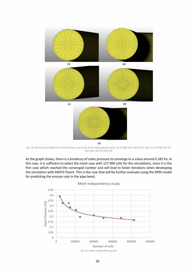
With the geometry set, 10 different meshes were created for the mesh independency analysis in order to evaluate the number of cells required until the static pressure shows an acceptable error. With that, it is sufficient to say that the simulations for predicting erosion rate will not be affected by the number of cells. Choosing the butterfly mesh type for the end surfaces and a swept hex-mesh for the volume, the number of cells starts from a coarse mesh with 18 800 cells, and it has been refined increasing the number of cells up to 414 528. The number cannot be increased further due to a limit of 500 000 cells for ANSYS Fluent student version used in this work. Fig. 18 shows how the surface of the inlet was refined during the independency analysis. A steady state model is used, combined with the turbulent model SST 𝑘 − 𝜔, which was found form the literature review that shows better results for erosion rate prediction. The numerical model Coupled was chosen to improve the convergence rate and a discretization scheme of second order was selected for better accuracy of iterations. The results for the mesh independency analysis are presented in the graph in Fig. 19.

26

Fig. 18: Illustration of different mesh densities used in the mesh independency study. (a) 18 800 cells, (b) 67 232 cells, (c) 127 000, (d) 251

856 cells, (e) 414 528 cells

As the graph shows, there is a tendency of static pressure to converge to a value around 0.185 Pa. In this case, it is sufficient to select the mesh case with 127 000 cells for the simulations, since it is the first case which reached the converged number and will lead to faster iterations when developing the simulation with ANSYS Fluent. This is the case that will be further evaluate using the DPM model for predicting the erosion rate in the pipe bend.

Fig. 18: Mesh independency graph

0

0.05

0.1

0.15

0.2

0.25

0.3

0.35

0.4

0.45

0 100000 200000 300000 400000 500000

Stat

ic P

ress

ure

(P

a)

Number of cells

Mesh independency study

27

3.3 Fluid flow model

After the mesh independency analysis, the next step for a CFD-based model is the flow modelling performed in a CFD software, in this case the ANSYS Fluent. To obtain the flow field, the calculations are mostly applied in engineering for a time-averaged form of Navier-Stokes, including the term for Reynolds stress, called RANS (Reynolds Averaged Navier-Stokes), shown by the Eqs. 19 – 20. There are different turbulent models, such as 𝑘 − 𝜀 and 𝑘 − 𝜔, offering closure equations. Each of these models has advantages and disadvantages there were evaluated in section 1.2.2 of this report. Since they provide flow field predictions at various conditions and geometries with different accuracy, it is important to choose an appropriate turbulence model [2]. The appropriate model should show a good convergence characteristic and be stable, with no changes in the coefficients for each flow. The equations for the turbulence model should also present a higher accuracy in a short time, using few transport equations. The models that will minimize time when solving RANS equation are the two-equations family 𝑘 − 𝜀 and 𝑘 − 𝜔. The 𝑘 equation is shown in Eq. 21 and presents the term to the left as and the second as the convection. The terms to the right correspond to the production, viscosity and turbulent diffusions, respectively.

𝜕

𝜕𝑥𝑗(𝜌𝑘𝑢�̅�) = 𝜇𝑇 (

𝜕𝑢�̅�𝜕𝑥𝑗

+𝜕𝑢�̅�

𝜕𝑥𝑖)𝜕𝑢�̅�𝜕𝑥𝑗

+𝜕

𝜕𝑥𝑗(𝜇 +

𝜇𝑇𝜎𝐾

𝜕𝑘

𝜕𝑥𝑗) − 𝜌𝜀

Eq. 21

The 𝜀 equation (Eq. 22) derives from Eq. 21, and the second term on the right corresponds to the production of 𝑘.

𝜕𝜌𝑢�̅�𝜀

𝜕𝑥𝑗=

𝜕

𝜕𝑥𝑗(𝜇 +

𝜇𝑇𝜎𝜀

𝜕𝜀

𝜕𝑥𝑗) + 𝐶𝜀1

𝜀

𝑘𝜇𝑇 (

𝜕𝑢�̅�𝜕𝑥𝑗

+𝜕𝑢�̅�

𝜕𝑥𝑖)𝜕𝑢�̅�𝜕𝑥𝑗

− 𝐶𝜀2𝜀

𝑘𝜌𝜀

Eq. 22

The constants for this equation when choosing the standard model on ANSYS Fluent are:

𝐶𝜇 = 0.09,𝜎𝑘 = 1.0,𝜎𝜀 = 1.3,𝐶𝜀1 = 1.44,𝐶𝜀2 = 1.92

However, the standard 𝑘 − 𝜀 presents issues for swirling and high shear flows. Alternatively, the CFD software presents the RNG 𝑘 − 𝜀 in order to solve the issue. The constants for RNG 𝑘 − 𝜀 are:

𝐶𝜇 = 0.0845,𝜎𝑘 = 0.72,𝜎𝜀 = 0.72,𝐶𝜀1 = 1.42,𝐶𝜀2 = 1.68

The additional term from the RNG 𝑘 − 𝜀 model is the following Eq. 23:

𝑅𝜀 =𝐶𝜇𝜌𝜂

3(1 − 𝜂 𝜂𝑜)⁄

1 + 𝛽𝜂3𝜀2

𝑘

Eq. 23

Where:

𝜂 =

𝑆𝜀

𝑘,𝛽 = 0.112,𝜂0 = 4.38

For 𝑘 − 𝜔, the 𝑘 equation remains the same, but the second equation used for calculation is as follows Eq. 24, considering a specific turbulence dissipation rate of 𝜔 = 𝜀/𝑘.

28

𝜕𝜌𝜔

𝜕𝑡+𝜕𝜌𝑢�̅�𝜔

𝜕𝑥𝑗=

𝜕

𝜕𝑥𝑗(𝜇 +

𝜇𝑇𝜎𝜔

𝜕𝜔

𝜕𝑥𝑗) + 𝐶𝜔1

𝜔

𝑘𝜇𝑇 (

𝜕𝑢�̅�𝜕𝑥𝑗

+𝜕𝑢�̅�

𝜕𝑥𝑖)𝜕𝑢�̅�𝜕𝑥𝑗

− 𝜌𝐶𝜔2𝜔2

Eq. 24

3.4 DPM sub-models In addition to solving transport equations for the continuous phase, ANSYS Fluent allows a simulation of a discrete second phase in a Lagrangian frame of reference. This second phase consists of spherical particles dispersed in the continuous phase. The simulation will compute the trajectories of these discrete phase entities, as well as heat and mass transfer to/from them. The coupling between the phases and its impact on both the discrete phase trajectories and the continuous phase flow can be also included [51]. The panel for the Discrete Phase Model contains the parameters related to the calculations for the discrete phase of particles. In order to perform coupled calculations of the continuous and discrete phase flow and simulate cases closer to experiment results, the interaction with the continuous phase needs to be engaged. This will enable an interaction between dispersed and continuous phases, in order words, the interaction between particle and fluid. A DPM iteration interval allows to control the frequency at which the particles are tracked and the DPM sources are updated. For the cases developed in this report, 20 iterations were set for the model. The tracking parameters contain settings to control the particle trajectories. The maximum number of time steps used to compute a single particle trajectory was set as default for 50 000 when using a steady-state particle tracking. The remaining settings in this panel were left as standard, previously defined by ANSYS Fluent. Several physical sub-models and forces are also available to be engaged to the CFD model in order to analyze and compare different results for erosion rate. Those options allow to simulate a wide range of discrete phase problems including particle separation and classification, spray drying, aerosol dispersion, bubble stirring of liquids, liquid fuel combustion, and coal combustion [51]. The ones selected in this report will be presented in depth in the next sections. 3.4.1 Erosion sub-model The erosion sub-model enables monitoring erosion and/or accretion rates at the wall boundaries. For the wall zone, a specific erosion model can be selected for calculations. In this report the model developed by Finnie is selected for the cases developed. The computation of the erosion rate is based on the real wall position and does not take into consideration variations of wall orientation for cases when a rough wall is present. Therefore, the conditions of the wall need to be taken into account for proper results. The boundary conditions can be mainly set as:

• Escape: The particle is simulated as have been escaped when encounters the wall zone, as illustrate in Fig. 19, and the trajectory calculations are, then, terminated;

29

Fig. 19: Particle trajectory for an escape boundary condition at the wall

• Trap: In the case of evaporating droplets or combustion particles, the volatile mass passes to the vapor phase and enters the cell adjacent to the boundary, shown in Fig. 20. The particle trajectory is terminated, and the particle is reported as trapped at the wall;

Fig. 20: Particle trajectory for a trap boundary condition at the wall

• Reflect: For this case, the particle will rebound off the wall with a change in its momentum. The wall surface can also be specified with the surface roughness parameter.

For this report, the boundary conditions at the wall were set as reflect with no rough wall, for means of simplification. When the reflect condition is chosen, two models are available from ANSYS Fluent for computing the change in the momentum of the particles: non-rotating particles or rotating particles. As a standard, non-rotating particles were set in the simulations. When creating the injection with sand particles, different parameters for a discrete phase injection can be defined. The injection type will be set as surface to create the injection in the inlet boundary in the pipe geometry. The particle type chosen is set as inert, for discrete phase element that obeys the force balance and can be subjected to heating or cooling [51]. The number of tries will control the inclusion of turbulent velocity fluctuations in the particle force balance. For the simulations performed, this value was set as 5, so there are enough particle trajectories added in the simulation. The material chosen to simulate sand particle is set as wood with a sand particle density of 2650 kg/m3, as experimental researches propose. For all simulations performed in this report, the particle is defined as non-spherical with a shape factor of 0.8 and a discrete random walk model is engaged. This model includes an instantaneous turbulent velocity on the particle trajectory through stochastic method. 3.4.2 Virtual mass force The virtual mass force will be engaged in the simulations for a comparison of results with the other sub-models described in this section. Using this force will add a new term in the equation of motion, Eq. 03, that will be included in the particle force balance. When the fluid density approaches or exceeds the particle density, it is recommended to engage this force in the simulations [51]. Although this is not case for this present report, since the fluid densities are below the particle density, the virtual mass will be selected as a matter of comparison, as it is a

30

phenomenon that will impact the particle trajectory and, therefore, cannot be neglected in a CFD model. 3.4.3 Stochastic collisions sub-model When engaging this sub-model from the DPM panel, the effect of collisions will be included in the simulations. It will, then, be considered the impacts of particle-to-particle collision. This sub-model assumes that the frequency of collisions is much less than the particle time step, and that the collisions will happen as a result of particles colliding at the wall and with each other. The coalescence sub-model is automatically engaged when the stochastic collision is selected. The coalescence of particles tends to cause spray to pull away from the wall [51]. For the purpose of this work, the coalescence was disabled. For the stochastic collisions sub-model, a transient simulation is used, multiple DPM iterations per time step cannot be specified in the DPM iteration interval, as well as the number of tries. The maximum number of time step changes automatically to 500 and the particle treatment is also impacted, due to the fact that the model changes to an unsteady particle tracking. Thus, the particle trajectory is capture for each particle as a single object in a specific time. With an unsteady particle tracking, it is important to add a start and stop time for the injections. With these values set to be zero, the sand particle injection will only occur at the beginning of the simulations, at t=0, and will not be repeated during the iterations.

31

4. Results In this section, it will be presented the results for a CFD simulation and empirical results for predicting erosion rate in a 90-degree pipe bend. The geometry created and described in section 3.2 is used in ANSY Fluent and placed vertically with the effect of gravity force acting in the system. The values for erosion rate presented are the maximum value obtained by the CFD simulations. For empirical results, the models API RP 14E and DNV GL RP O501 were used, and the results found are compared with CFD, as well as with experimental data in order to validate the simulations performed.

4.1 Case 1 – Gas and sand particles

The first case developed have the parameters chosen based on an experimental work performed by Chen et al. in 2006 [48], where gas flow carrying sand particles were conducted inside a pipe of aluminum with a diameter of 25.4 mm, as shown in the sketch in Fig. 21. The radius of curvature in this experiment is 1.5D.

Fig. 21: Schematic sketch for an elbow used in the experimental work [48]

The sand particles had a diameter of 250 𝜇m and were added continuously in the system with a flow rate of 3.0⋅10-4 kg/s, the air had a fluid velocity of 45.72 m/s. Table 05 below presents a summary of the parameters used in this simulation.

Table 05: Parameters for simulating air and sand particles based on experimental work [48]

Parameter Unit Value

Particle diameter 𝜇m 250

Wall material density (Aluminum) kg/m3 2719

Fluid velocity m/s 45,72

Flow rate kg/s 3,0E-04

Pipe diameter mm 25,4

Particle density kg/m3 2650

Using the Eq. 04 previously presented, and a viscosity for air as 1.225 kg/m⋅s, the value found for the Re number is 113 025. With that, it can be said that the system is in a turbulent flow regime, since the Re is above 4 000, as indicated before in Fig. 10. In order to verify the coupling effect investigated by Elghobashi, the particle for this case has a volume fraction of 1.44⋅10-4. The Stokes number found, considering a ratio between particle response time, 𝜏𝑣, and the characteristic time flow, 𝜏𝑓, given in Eq. 25, is approximately 1 000.

32

𝑆𝑡 =

𝜏𝑣𝜏𝑓

Eq. 25

Looking at the graph from Fig. 09, this presented system is a two-way coupling in the area number 2 indicated in the graph, where the particles enhance turbulence. This is the case where the particle loading is sufficiently high, causing the particle phase to largely affect the fluid phase. 4.1.1 Analysis of models Based on the experiment developed by Chen et al. in 2006 [48], the erosion sub-model was selected to create the Case 1A presented in the graph below (Fig. 22). For the Case 1B, a virtual mass force is engaged together with the erosion sub-model, to analyze the variation in the erosion rate in the elbow. Case 1C is created engaging erosion and stochastic collisions in the DPM model. And, finally, Case 1D is created engaging all forces and sub-models used previously. Erosion, virtual mass force and stochastic collisions are all enabled in this case to analyze the results. Both empirical models, API RP 14E and DNV GL RP O501, were used to calculate and predict the erosion rate in the elbow. All results found are compared below.

Fig. 22: Erosion rate for gas and sand particles, (Case 1A) erosion sub-model engaged, (Case 1B) erosion and virtual mass force engaged,

(Case 1C) erosion and stochastic collision sub-models engaged, (Case 1D) erosion, virtual mass force and stochastic collision models engaged, empirical model DNV GL RP O501 and API RP 14E

It can be seen from Fig. 22 that there is a tendency in lowering the erosion rate when considering the erosion sub-model combined with virtual mass force and stochastic collision put together, than when engaging only the erosion the sub-model. The decrease when engaging the stochastic collisions to the simulation is due to the fact that, now, the iterations performed will take into account, not only the particle-to-wall collisions, but also particle-to-particle collisions. In this case, it is verified that when these collisions are enabled, the erosion rate tend to decrease, showing now difference when added virtual mass to the model, since the erosion rates found for Cases 1C and 1D are the same. The empirical DNV model shows a lower value for erosion rate but in the same order as the results found for CFD. However, the API model presents a much smaller rate for erosion, due to the fact that is a simpler model that does not take into consideration the type of geometry used and other parameters, such as particle and pipe diameters, fluid velocity, density as well as viscosity.

33

In order to compare the CFD results with the experiment performed, the contour of erosion rate in the wall is used for this matter. Both cases, Case 1A, with the highest erosion rate, and Case 1D, with the lowest erosion rate found in the CFD model are compared with the contour found for the experiment developed by Chen et al and it is presented in Fig. 23.

Fig. 23: Erosion rate in the elbow (a) experimental result [48], (b) CFD result Case 1A, (c) CFD result Case 1D

The three results show that the maximum erosion rate occurs in the corner region of the elbow. Both CFD cases do not present a significant change in the area with maximum erosion, showing that this is not impacted by the different sub-models selected in each simulation. Therefore, CFD analysis can bring results predicting the area of maximum erosion similarly to the one found in the experiment. The CFD simulation files for the cases developed with gas and sand particles, are presented in Fig. B1 – Fig. B4 of the Appendix B. 4.1.2 Parametric study The CFD cases developed for a parametric study are calculated engaging the DPM model with the erosion sub-model in ANSYS Fluent. For comparison, both turbulence models RNG 𝑘 − 𝜀 and SST 𝑘 −𝜔 were chosen to have the results evaluated. For the experimental work, the sand particle had a diameter of 250 𝜇m, but to develop a parametric study, other simulations were performed with particle diameters of 50, 150, 350 and 450 𝜇m. Cases 1E – 1I were created in order to analyze the effect of particle diameter in relation to erosion rate in the elbow. The analyzes are presented in the graph shown in Fig. 24.

Fig. 24: Effect of particle size and turbulence models in erosion rate

1.30E-04

1.40E-04

1.50E-04

1.60E-04

1.70E-04

1.80E-04

1.90E-04

50 𝜇m 150 𝜇m 250 𝜇m 350 𝜇m 450 𝜇m

Ero

sio

n r

ate

(kg/

m2⋅s

)

Effect of particle size and turbulence model

SST k-ω RNG k-ε

34

The graph above shows, as investigated by Desale et al. [35], that the erosion rate in the pipe bend can be influenced by the particle size diameter. Desale et al. concluded that for higher particle diameters, the erosion rate would also increase. However, the CFD analysis show that there is an increase in the erosion rate when the particle diameter increases from 50𝜇m to 150𝜇m, reaching its maximum and appearing to be constant for particle sizes over 150 𝜇m. For the turbulence models, the results show an agreement between 97%-99% with the erosion rate. With that, it can be said that the choice for turbulence models will not have a drastically impact in the erosion rate calculations. Therefore, the SST 𝑘 − 𝜔 will be the model selected for future analyzes. The erosion rate found for each case, is summarized in Table A1 of Appendix A and the CFD simulation files can be viewed in Appendix B, Fig. B5 – Fig. B14. Evaluating the velocity parameter, the next results show the cases created, Cases 1J – 1N, for the erosion rate with gas velocities of 25, 35, 45.72, 55 and 65 m/s. The SST 𝑘 − 𝜔is used with the DPM model engaged and the erosion sub-model selected for the CFD simulations. The particle diameter is 250 𝜇m, as in the experimental work. The results found in this analysis are compared with the DNV GL RP O501 empirical model and presented in Fig. 25. The API model could not be used for comparison, as its approach does not consider the fluid velocity as an input.

Fig. 25: Effect of gas velocity in erosion rate for CFD and DNV GL RP O501

As the figure above shows, the erosion rate increases when the air velocity increases. This can be explained by the fact that with a higher fluid velocity, the particles will impact the wall at a higher speed. This shows a direct relation between particle impact velocity and erosion rate. The results found for the empirical model follow the same trend as CFD, showing an agreement in both approaches used. The erosion rate found for each case, is summarized in Table A2 of Appendix A and the CFD simulation files can be viewed in Appendix B, Fig. B15 – Fig. B19.

0.00E+00

5.00E-05

1.00E-04

1.50E-04

2.00E-04

2.50E-04

3.00E-04

3.50E-04

4.00E-04

25 m/s 35 m/s 45,72 m/s 55 m/s 65 m/s

Ero

sio

n r

ate

(kg/

m2⋅s

)

Velocity effect in gas fluid

CFD DNV

35

4.2 Case 2 – Water and sand particles

Another experimental work was chosen for comparison in this present report to analyze the erosion rate with a water fluid carrying sand particles. The work was performed by Shirazi et al. [50] in 2021. The experiment was created with a pipe diameter of 50.8 mm made of steel, with a density of 7800 kg/m3, and a radius of curvature in a 90° elbow of 1.5D. The fluid had a velocity of 6.3 m/s and a flow rate of sand particles of 0.1285 kg/s with particles with a diameter of 300 𝜇m. The geometry used for Shirazi et al. is illustrated in Fig. 26. The parameters used in this simulation are summarized in Table 06.

Fig. 26: Geometry used for the experimental work with water and sand particles [50]

Calculating the Reynolds number as shown in Eq. 04, using the fluid viscosity as 998.2 kg/m⋅s, it is found the value of 318 508. This means that the system is in the turbulence flow regime, since it has a value above 4 000. To evaluate the coupling effect using the Eq. 25 for the Stokes number, it is calculated a value of 1.64. The particle volume fraction, 𝛼𝑝, is 0.146 and it indicates that the case

presented is a four-way coupling with a dense suspension, since the particles have a significant diameter. In the case of dense flows, it is expected that the particle-to-particle interaction will affect both the particle and the fluid phase.

Table 06: Parameters for simulating water and sand particles based on experimental work [50]

Parameter Unit Value

Particle diameter 𝜇m 300

Wall material density (Aluminum) kg/m3 7800

Fluid velocity m/s 6,3

Flow rate kg/s 0,1285

Pipe diameter mm 50,8

Particle density kg/m3 2650

36

4.2.1 Analysis of models The results found in CFD for erosion rate are obtained from the maximum erosion found after the iterations, engaging the model described by Finnie available in ASNYS Fluent. Case 2A is created engaging the erosion sub-model as a start. Afterwards, virtual mass force is engaged combined with the erosion sub-model to create the Case 2B. Case 2C is performed its calculation engaging the erosion sub-model and the stochastic collisions, to verify how the particle-to-particle collisions will affect the prediction of erosion rate. Finally, the last Case 2D is developed engaging the erosion sub-model, the virtual mass force and the stochastic collisions. Those cases are, then, compared with the experimental results obtained by Shirazi et al. and with the empirical models, DNV GL RP O501 and API RP 14E, presented in Fig. 27.

Fig. 27: Erosion rate for water and sand particles, (Experiment 2) result from experimental work [50], (Case 2A) erosion sub-model

engaged, (Case 2B) erosion and virtual mass force engaged, (Case 2C) erosion and stochastic collision sub-models engaged, (Case 2D) erosion, virtual mass force and stochastic collision sub-models engaged

The results found for CFD show that engaging more sub-models and forces to the simulation, the erosion rate tends to decrease. Cases 2B and 2C have erosion rate similar to the result found in the experiment mentioned. That indicates that for a more realistic result, either virtual mass or stochastic collision needs to be engaged in the CFD model. The empirical model calculated using the API equation has a good accordance with Case 2D, when all forces are engaged. The DNV model showed an erosion rate 5 times higher than the Case 2A, which was the highest result for the CFD simulations. A discrepancy is also verified when comparing with the other models, indicating that the DNV overpredicts the erosion for the case of water and sand particles. The erosion rate found for each case, is summarized in Table A3 of Appendix A and the CFD simulation files can be viewed in Appendix B, Fig. B20 – B23. Analyzing the particle trajectory, a difference can be seen when different sub-models are selected. As Fig. 28 shows, there is a different way in calculating the particle trajectories when the stochastic sub-model is engaged. This is due to the fact that for stochastic collisions, an unsteady particle trajectory is simulated. In this case, the location of a particle released from the inlet at a specific time is simulated. Therefore, a picture of the trajectory of the sand particle is taken on the exact moment they reach the pipe bend. Several simulations were carried out in order to picture the moment when a highest erosion rate is reached in the 90° elbow. In such case, a comparison between the sub-models for the particle trajectory is not possible, due to the fact that the calculations and the simulation were made in different ways.

1.49E-05 1.29E-058.39E-06

3.47E-061.02E-05

1.02E-06

7.49E-05

0.00E+00

1.00E-05

2.00E-05

3.00E-05

4.00E-05

5.00E-05

6.00E-05

7.00E-05

8.00E-05

Case 2A Case 2B Case 2C Case 2D Experiment2

Empirical(API)

Empirical(DNV)

Ero

sio

n r

ate

(kg/

m2 ⋅

s)

Erosion rate

37

Fig. 28: Particle trajectory, (a) erosion sub-model engaged, (b) erosion and virtual mass force engaged, (b) erosion and stochastic collision

sub-models engaged, (d) erosion, virtual mass force and stochastic collision sub-models engaged

Since Fig. 27 indicates that Cases 2B and 2C have a more alignment with the experiment performed, the profile for maximum erosion is used for comparison for both cases with the profile created by Shirazi et al., showed in Fig. 29. The figure presents, as mentioned previously, that for Case 2C with the erosion and the stochastic sub-models engaged, the area for erosion cannot be compared with the other methods, due to different approach and unsteady particle tracking for the stochastic collision sub-model. While Case 2B indicates a similar profile as the experiment result, with the maximum erosion rate occurring towards the end of the elbow. The CFD simulates an area with maximum erosion closer to a realistic result found in the experiment when the virtual mass force is engaged together with the erosion sub-model.

Fig. 29: Erosion rate in the elbow (a) experimental result [50], (b) CFD result Case 2B, (c) CFD result Case 2C

38

4.3 Case 3 – Water and sand particles

To develop another simulation for water carrying sand particles in order to verify once more the prediction of erosion rate from CFD and empirical models in relation to experiments, Case 3 is developed based on an experimental work performed by Wee and Yap [49] to recreate the practice in a CFD context in ANSYS Fluent for a fluid with water carrying sand particles. In this experiment, they have analyzed the impact of the water velocity considering 11, 15, 23 and 27 m/s, with sand particles with a diameter of 150 𝜇m entering the pipe with a bend of 90°. The set-up is illustrated in Fig. 30. The radius of curvature used in this experiment is 1.5D. A summary with the parameters used in all CFD cases performed in this section are presented in Table 07.

Fig. 30: Geometry used for the experimental work with water and sand particles [49]

The Re number calculated for this case is 2 047 554 for a water velocity of 27 m/s, and 834 119 for the lowest velocity used in the simulation of 11 m/s. Thus, all cases developed in this section are in a turbulent flow regime. For the Stokes number, found using Eq. 25, the value is 1.1702 and the particle volume fraction is 1.547⋅10-4. With these values found, the system is found to be a two-way coupling in the area number 3 of Fig. 09, represented by Elghobashi. That is the case where smaller particles will promote a turbulence dissipation.

Table 07: Parameters for simulating water and sand particles based on experimental work [49]

Case name Particle

Diameter (𝜇m)

Wall material density

(Aluminum) (kg/m3)

Fluid velocity

(m/s)

Flow rate (kg/s)

Pipe diameter (mm)

Particle density (kg/m3)

Case 3A – 11 150 2719 11 0,00294 76,2 2650

Case 3A – 15 150 2719 15 0,00274 76,2 2650

Case 3A – 23 150 2719 23 0,00297 76,2 2650

Case 3A – 27 150 2719 27 0,00238 76,2 2650

39

4.3.1 Analysis of models For all CFD analyzes, the SST 𝑘 − 𝜔 was chosen as the turbulence model. Selecting the DPM model and engaging together with different sub-models and forces available on ANSYS Fluent, 16 different cases were created for a comparison of the results within a CFD context as well as with experimental results found in literature. Cases 3A were created engaging only the erosion-sub model. While Cases 3B were created engaging, not only the erosion sub-model, but also the virtual mass force, to be added at the equation of motion. Cases 3C, were built with the stochastic collision sub-model together with the erosion sub-model. Lastly, the simulation for Cases 3D were performed with all forces from previous cases to verify the difference in the erosion rate from different sub-models at different velocities. The results are, then, presented in Fig. 31.

Fig. 31: Velocity effect with CFD. (Experiment 3) result from experimental work [49], (Case 3A) erosion sub-model engaged, (Case 3B)

Erosion and virtual mass force engaged, (Case 3C) erosion and stochastic collision sub-models engaged, (Case 3D) erosion, virtual mass force and stochastic collision sub-models engaged

In the graph above, the analyzes made on ANSYS Fluent present the expected, with the erosion rate increasing while the water velocity increases. All CFD cases follow the trend found in the experiment until the velocity reaches 23 m/s. At 27 m/s, the erosion rate for the experimental work has a lower value than the CFD cases. For the highest velocity, Cases 3C and 3D are the ones that can predict the erosion much closer to the one found by Wee and Yap. This can be explained by the presence of the stochastic collision sub-model in the simulation. When this model is not engaged, the erosion rate has higher values. Hence, for more realist results, it needs to be taken into account the particle-to-particle collision at higher velocities. Since the particles will hit the wall more significantly at a higher kinetic velocity and will collide to each other. The erosion rate found for each case, is summarized in Table A4 of Appendix A and the CFD simulation files can be viewed in Appendix B, Fig. B24 – B39. Cases 3A, with the erosion sub-model engaged, were selected for comparison with empirical models, DNV GL RP O501 and API RP 14E at different fluid velocities. See the results in Fig. 32. The API equation does not consider the fluid velocity as an input parameter, that is way a constant value is shown for the model in the figure below for all four velocities used.

0.00E+00

5.00E-07

1.00E-06

1.50E-06

2.00E-06

2.50E-06

11 m/s 15 m/s 23 m/s 27 m/s

Ero

sio

n r

ate

(kg/

m2⋅s

)

Velocity effect in water fluid

Case 3A

Case 3B

Case 3C

Case 3D

Experiment 3

40

Fig. 32: Effect of water velocity in erosion rate comparing experiment and CFD results

The DNV model follows the tendency found in CFD and experimental results, until 23 m/s. However, for means of comparison, the erosion rate for this empirical model needed to be multiplied by a factor of 0.1 in order to be in the same order as the other results obtained. The DNV model also overpredicts the erosion rate at higher velocities, as the cases performed in CFD showed. This empirical model cannot represent the particle-to-particle interactions and that is why is not similar to realistic results when the particles have a higher kinetic velocity. The erosion rate calculated using the API empirical model maintains constant, since this model has a limitation and does not consider the fluid velocity. Therefore, it cannot replicate the rate at different fluid velocities, but the value obtained is in the same order as the erosion rate found in the other models. Fig. 33 below presents the erosion rate at the wall in the pipe bend for all different velocities used for the simulation for Case 3A. It shows the areas in the elbow where the maximum erosion rate occurs, and it can be seen how the areas that are most impacted by the sand particles change with the velocity.

Fig. 33: Erosion rate in the elbow. (a) water velocity of 11 m/s, (b) water velocity of 15 m/2, (c) water velocity of 23 m/s, (d) water velocity

of 27 m/s

0.00E+00

5.00E-07

1.00E-06

1.50E-06

2.00E-06

2.50E-06

3.00E-06

11 m/s 15 m/s 23 m/s 27 m/s

Ero

sio

n r

ate

(kg/

m2 ⋅

s)

Chart Title

Experimental CFD Empirical (DNV) (*0,1) Empirical (API)

41

The red areas in the pictures increase in number and get wider with the increase of velocity. This is also indicated in the graph from Fig. 32, when it can be seen that the erosion rate increases with the increase of velocity. Fig. 34 illustrates the same contour for the elbow found in the experiment developed by Wee and Yap [49]. In this figure, it can be noticed that the area for a maximum erosion rate is in a vee-shaped erosion scar. The same was not seen in the CFD simulations. Therefore, the profile with the area in the wall with maximum erosion rate obtained in the CFD model cannot be compared with the experimental result.

Fig. 34: Erosion rate in the elbow for the experimental work [49]

42

5. Discussion

This project for a master thesis aimed to investigate erosion rate for a 90-degree pipe bend using the CFD model with ANSYS Fluent, and a comparison between the experimental data found in literature, as well as with the empirical models API RP 14E and DNV GL RP O501. This report investigated the influences of type of fluid, fluid velocity, pipe diameter and particle diameter in predicting the erosion rate and the results obtained on a CFD and empirical contexts towards a realistic result found in a controlled environment. For the first case performed, with air and sand particles, the Case 1D, with only the erosion sub-model engaged, was the case which presented a closer result with the empirical study. In is presented in Fig, 35 that the erosion rate found from DNV showed an accordance of 72% with the CFD model. The API instead, showed only 18%. This empirical model presents limitations that impact the results when compared with more complex models. The approach for predicting the erosion rate does not consider the pipe geometry, the particle diameter, neither the fluid velocity. Also, the empirical constant used in this model, the 𝐶 value, is not well defined for fluids carrying solid particles. The experimental result for gas and sand particles was compared to the CFD cases using the erosion profile at the wall as a method of comparison. This showed that the area where the maximum erosion occur is in the same region for both approaches and it is encountered at the end of the elbow with a vee-shaped erosion scar. The turbulence models, SST 𝑘 − 𝜔 and RNG 𝑘 − 𝜀, were also investigated in the CFD context, showing that no significant changes occur in the erosion rate. Therefore, both turbulence models could be used for the analyzes made in this report. The particle diameter was also analyzed to comprehend the effect in the erosion rate. This study showed that the erosion rate reached a maximum value at a particle size of 150 𝜇m and at higher values, it remained constant. The velocity effect was also investigated, comparing the CFD results with the DNV GL RP O501 empirical model. Both methods followed the same tendency, where the erosion rate increases with the increase of velocity.

Fig. 35: Erosion rate for experimental, DNV, API and best cases in CFD

For the second case developed where water at a velocity of 6,3 m/s carries sand particles, the CFD result for the Case 2D has a much similar value in comparison with the experimental result and the API empirical model. However, Fig, 35 shows that both CFD and API underpredict the erosion rate encountered in a controlled environment for the experimental work performed. Using the DNV approach, the value for erosion overpredicts for a realistic case, which shows that this model can be used for predicting the erosion rate, since it gives a more conservative result.

1.02E-051,37E-06

1,61E-04

3.47E-06 1,73E-06

1,15E-04

7.49E-05

1,84E-05

2,90E-05

1.02E-06 1,02E-06

Case 1D Case 2D Case 3A at 23 m/s

Ero

sio

n r

ate

(kg/

m2 ⋅

s)

Erosion rate for different cases

Experiment CFD DNV API

43

The profile of erosion rate found in CFD was verified with the experiment result. This study showed that both contours at the pipe wall were similar in both approaches, showing that the maximum erosion rate is found at the end of the elbow. Finally, the last case performed was a flow with water at different velocities, 11, 15, 23 and 27 m/s, carrying sand particles. Several cases were created in CFD in order to compare with the results found in the experiment used for benchmarking and with the empirical models. Fig. 35 illustrates the erosion rate results for all the approaches used. For the DNV model, the result obtained, showed that this model overpredicts the erosion rate when compared to a realistic scenario. More accordance with the results were found using the API empirical model and the CFD simulation, showing that those approaches can predict the erosion rate similar to reality. The fluid velocity was also investigated in this case. Although the API RP 14E model does not include the velocity of the carrier fluid as an input parameter, the results showed a great accordance with the experiment and CFD. It could be noticed that the methods followed the tendency of the experiment data until the velocity reaches 23 m/s. After this value, there is a decreased in the erosion rate from the experimental work and CFD and empirical models gave higher values. The Case 3A created in ANSYS Fluent, used only the erosion sub-model engaged to the simulation. That can explain the higher values found with the CFD simulation. For higher velocities, the stochastic collision could bring better results, since this model would take into consideration the particle-to-particle collision. Having higher velocities, the sand particles will impact the wall more significantly and would collide with one another. With more interaction between particles, the particle-to-wall collisions would decrease, and the erosion rate would have lower results. In this case, the profile for erosion rate occurred at the pipe wall was also investigated. The results found from CFD were compared with the experimental data. This study showed that the maximum erosion rate found in the experiment had a vee-shaped erosion scar in the elbow. However, the same pattern could not be identified in the simulations performed with ANSYS Fluent. Taking in to account all cases presented in Fig. 35, it can be seen that the flow carrying the smaller sand particles, Case 3 with particle size of 150 𝜇m, shows the lowest erosion rate. As investigated by Tilly [9], the erosion rate does not change after a solid particle diameter larger than 100 𝜇m. However, in this present report, Cases 1, particle size of 250 𝜇m and 2, particle size of 300 𝜇m, showed values of 100 and 10 order of magnitude, respectively, larger than Case 3. A gas flow, with air that has a density of 1.225 kg/m3, also provides the highest values found for erosion rate in a 90-degree pipe bend when compared to liquid flow, with water that has a density of 998.2 kg/m3, for a particle with 2650 kg/m3 of density. This shows that when the continuous phase has a density much lower than the solid particles, the erosion rate is more significant. Whereas, if the continuous phase has a velocity that nearly reaches the density of the dispersed-phase, the erosion rate reduces its value.

44

6. Conclusion

The project presented in this paper was part of a master thesis project in collaboration with Ramboll. The aim of this work was to investigate the possibility of predicting erosion ate using CFD for flows carrying sand particles in a 90-degree pipe bend. This case was brought from Ramboll, since it is a relevant concern from oil and gas industries. The presence of solid particles can cause blockage inside pipes, removing of materials as well as corrosion. CFD can help understand the phenomenon happening in the pipe, the forces acting in the particle and predict an erosion rate to improve the lifespan of the pipe. Elbows are a critical type of geometry that will allow erosion to occur, that is why this geometry was selected for the present study. To define the problem statement of this project, two questions were raised: “Can erosion models based on CFD predict erosion rate when compared to a precisely controlled experimental study?” “Are erosion models based on CFD superior to the most widely used empirical models?” To answer these questions, three different cases were created to compare single-phase flows, with air and water, engaging the Euler-Lagrangian approach with different sub-models available in ANSYS Fluent. Parametric studies were also performed in order to investigate and verify how the erosion rate can change in the 90-degree pipe bend. According to the literature review found in the work performed by Desale at al. [35], and also presented in the simulations performed, an increase in particle diameter influences the erosion rate, increasing its value, for sand particle diameters up to 150 𝜇m. Larger particles will impact the wall in a more significant way then smaller particles, even if they have the same velocity. For diameters above this value, the erosion rate showed to be constant and is not impacted by the particle size. This is also verified in the work written by Tilly [9], who concluded that for particles above 100 𝜇m the erosion rate is nearly independent of the particle size. The fluid velocity is also another important parameter that was investigated in this report. For higher velocities, the particles would impact the target wall more having a higher kinetic energy, therefore the erosion rate becomes more significant. That was verified in the Case 3 with water carrying sand particles at 4 different velocities, 11 m/s, 15 m/s, 23 m/s and 27 m/s, comparing the CFD model and the DNV empirical model. However, the experiment work showed that at the highest velocity, the erosion model would decrease. This can be explained by the fact that the CFD and empirical models, did not take into account the effect of particle-to-particle collision to engage the stochastic collision sub-model. In this case, these collisions that could reduce the erosion, were not taken into consideration. Comparing both Cases 2 and 3, where water was the continuous phase, the higher particle flow rate was used in Case 2, 0.1285 kg/s. Case 3, in the other hand, had flow rates between 0.00238 kg/s and 0,00297 kg/s. The present work showed that with a higher particle concentration, the erosion rate encountered in the elbow is more relevant than when lower concentrations are used. With all the analyses performed in this work, the first answer for the problem state can be answered. With the results presented, it can be concluded that CFD can predict the erosion rate similarly to the experimental works used as benchmarking in the report. Cases 2 and 3 with water, had similar results

45

between CFD and the experiments used in the report. For Case 1 using air with sand particles, the profile of erosion rate in the pipe wall showed that the maximum erosion rate is encountered in the same location, the elbow surface, in both CFD and experiment results. The DNV GL RP O501 overpredicted the results for water and sand particles, when compared to CFD, API and experiment. Thus, this is a method that can also be used for analyses of erosion rate, since it gives more conservative results. The API RP 14E, despite the fact that is a simple approach and does not consider input parameters as fluid velocity, pipe geometry and particle size, it was the model that presented results similar to the experiment ones but in all three cases created, underpredicting the erosion ate for a 90-degree pipe bend. To use this model, a better understanding needs to be made to evaluate the relevance of using the empirical API model for predicting the erosion rate. Answering the second question raised in the problem statement, the CFD results found in Cases 2 and 3, showed better results than empirical models, when compared to the results obtained from the experiments. Therefore, it is beneficial to use CFD analysis for predicting erosion rate, since it is a method that can bring results closer to a realistic scenario. As for empirical models, it needs to be stated that API underpredicts the results, since it is a simple approach, while DNV showed to overpredict the erosion rate for a 90-degree pipe bend.

46

Bibliography

[1] Larsen, A. S., “Sand particle erosion in 90-degree pipe bends”, 2020. [2] Parsi, M., et al., 2014; “A comprehensive review of solid particle erosion modelling for oil and gas wells and pipelines applications”, Journal of Natural Gas Science and Engineering, 850-873. [3] Tang, N., Gomboc, J., “CFD modelling and experimental verification of erosion in a pipe bend by water flow transported solid particles”, 2017. [4] Pouraria, H., et al., 2020; “CFD modelling of the influence of particle loading on erosion using dense discrete particle model”, Wear, 460-461. [5] Finnie, I., 1960; “Erosion of surfaces by solid particles”; Wear, 87-103. [6] Bitter, J., 1963; “A study of erosion phenomena part I”, Wear, 5-21. [7] Bitter, J., 1963; “A study of erosion phenomena part II”, Wear, 169-190. [8] Neilson, J., Gilchrist, A., 1968; “Erosion by a stream of solid particles”, Wear, 11-122. [9] Tilly, G., 1973; “A two stage mechanism of ductile erosion”, Wear, 87-96. [10] Brach, R., “Impact dynamics with application to solid particle erosion”, 1988. [11] Sundararajan, G., 1991; “A comprehensive model for the solid particle erosion of ductile materials”, Wear, 111-127. [12] Coffin, L., 1954; “A study of the effect of cyclic thermal stress on a ductile metal”, Trans. ASME, 931-950. [13] Manson, S., “Behavior of materials under conditions of thermal stress”, 1953. [14] Salama, M. M., Venkatesh, E. S., “Evaluation of API RP 14E erosional velocity limitations for offshore gas wells”, 1983. [15] Salama, M. M., “An alternative to API 14E erosional velocity limits for sand laden fluids”, 1998. [16] Svedeman, S. J., Arnold, K. E., 1994; “Criteria for sizing multi-phase flow lines for erosive/corrosive services”, SPE Prod. Facil, 74-80. [17] API, 1981; “API RP 14E Recommended practice for design and installation of offshore production platform piping systems”, 3rd Edition, American Petroleum Institute, 22. [18] Det Norske Veritas, “Recommended practice RP O501: Erosive wear in piping systems”, 1996. [19] Duarte, C. A. R., et al., 2015; “Numerical investigation of mass loading effects on elbow erosion”, Powder Technology, 593-606. [20] Lain, S., Sommerfeld, M., 2015; “Parameters influencing dilute-phase pneumatic conveying through pipe systems: A computational study by the euler/lagrange approach”, The Canadian Journal of Chemical Engineering, 1-17. [21] Duarte, C. A. R., et al., “Effects of surface roughness and inter-particle collisions on elbow erosion”, 2016. [22] Mansouri, A., et al., 2014; “A combined CFD/experimental methodology for erosion prediction”, Wear, 332-333:1090-1097. [23] Mansouri A., et al., 2015; “Improved CFD modelling and validation of erosion damage dure to fine sand particles”, Wear, 338-350. [24] Kim, H., et al., 2015; “Simulation of solid particle erosion in wc-ni coated wall using CFD”, Journal of Materials Processing Technology, 240-245. [25] Abdulla, A., “Estimating erosion in oil and gas pipe line due to sand presence”, 2011. [26] Munson, B. R., et al., 2013; “Fundamentals of fluid mechanics”, 7th Edition, 416. [27] Holland, F. A., Bragg, R., “Fluid Flow for Chemical Engineers”, 1995. [28] Jordan, K., “Erosion in multiphase production of oil & gas”, 1998. [29] Chen, X., et al., 2006; “A comprehensive procedure to estimate erosion in elbows for gas/liquid/sand multiphase flow”, Energy Resour. Technol., 70-78. [30] McLaury, B. S., Shirazi, S. A., 2000; “An alternative method to API RP 14E for predicting solids erosion in multiphase flow”, Energy Resour. Technol., 115-122. [31] Pudasaini, S. P., 2019; “A fully analytical model for virtual mass force in mixture flows”, International Journal of Multiphase Flow, 142-152.

47

[32] Brennen, C. E., “A review of added mass and fluid internal forces”, 1982. [33] Levy, A., Chik, P., 1983; “The effect of erodent composition and shape on the erosion of steel”, Wear, 151-162. [34] Gandhi, B. K., Borse, S. V., 2002; “Effect of particle size and size distribution on estimating erosion wear of cast iron in sand-water slurries”, Indian J. Eng. Mater. Sci., 480-486. [35] Desale, G. R., Gandhi, B. K., Jain, S. C., 2009; “Particle size effects on the slurry erosion of aluminum alloy (AA 6063)”, Wear, 1066-1071. [36] Elghobashi, S., 1994; “On predicting particle-laden turbulent flows”, Applied Scientific Research, 309-329. [37] Levy, A., Hickey, G., 1982; “Surface degradation of metals in simulated synthetic fuels plant environments”, International Corrosion Forum, 154. [38] Brown, R., Jun, E. J., Edington, J. W., 1981; “Erosion of 𝛼-Fe by spherical glass particles”, Wear, 347-363. [39] Deng, T., et al., 2005; “Effect of particle concentration on erosion rate of mild steel bends in a pneumatic conveyor”, Wear, 480-487. [40] Sheldon, G., 1970; “Similarities and differences in the erosion behavior of materials”, J. Basic Eng. Trans. ASME, 619-626. [41] Kannojiya, V., Deshwal, M., Deshwal, D., “Numerical analysis of solid particle erosion in pipe elbow”, 2018. [42] Barton, N. A., “Erosion in elbows in hydrocarbon production systems: Review document”, 2003. [43] Nesic, S., Huizinga, S., “Review of the API RPP 14E erosional velocity equation: Origin, applications, misuses and limitations”, 2019. [44] HSE Health & Safety Executive, “Erosion in elbows in hydrocarbon production systems: Review document”, 2003. [45] DNVGL-RP-O501, “Managing sand production and erosion”, 2015. [46] Det Norske Veritas, “Recommended practice RP O501: Erosive wear in piping systems”, 2007. [47] Versteed, H. K., Malalasekera, W., 2007, “An introduction to computational fluid dynamics”, 2nd Edition, 10-20. [48] Chen, X., McLaury, B. S, Shirazi, S. A., 2006; “Numerical and experimental investigation of the relative erosion severity between plugged tees and elbows in dilute gas/solid two-phase flow”, Wear, 715-729. [49] Wee, S. K., Yap, Y. J., 2019; “CFD and experimental study of sand erosion in pipeline”, Journal of Petroleum Science and Engineering, 269-278. [50] Shirazi, S. A., Bilal, F. S., Sedrez, T. A., 2021; “Experimental and CFD investigations of 45 and 90 degrees bends and various elbow curvature radii effects on solid particle erosion”, Wear, 36-46. [51] ANSYS Fluent – User Guide, 2021, 2311-2490.

48

Appendix A – Tables

Table A1: Parameters and case names for the parametric study with particle diameter

Case name Particle

Diameter (𝜇m) Erosion rate

(kg/m2⋅s)

Case 1E - RNG k-𝜀 50 1,53E-04

Case 1E - SST k-𝜔 50 1,50E-04

Case 1F - RNG k-𝜀 150 1,85E-04

Case 1F - SST k-𝜔 150 1,82E-04

Case 1G - RNG k-𝜀 250 1,78E-04

Case 1G - SST k-𝜔 250 1,84E-04

Case 1H - RNG k-𝜀 350 1,77E-04

Case 1H - SST k-𝜔 350 1,79E-04

Case 1I - RNG k-𝜀 450 1,77E-04

Case 1I - SST k-𝜔 450 1,78E-04

Table A2: Parameters and case names for the parametric study with gas velocity

Case name Gas velocity

(m/s) Erosion rate

(kg/m2⋅s) - CFD

Erosion rate (kg/m2⋅s) - DNV

Case 1J 25 5,64E-05 2,40E-05

Case 1K 35 1,11E-04 5,76E-05

Case 1L 45,72 1,85E-04 1,15E-04

Case 1M 55 2,69E-04 1,87E-04

Case 1N 65 3,73E-04 2,88E-04

Table A3: Erosion rate found for Case 2

Model Erosion rate

(kg/m2⋅s)

CFD – Case 2A 1,49E-05

CFD – Case 2B 1,29E-05

CFD – Case 2C 8,39E-06

CFD – Case 2D 3,47E-06

API 1,02E-06

DNV 7,49E-05

49

Table A4: Parameters and erosion rate found for Case 3

Case name Erosion rate

at 11 m/s (kg/m2⋅s)

Erosion rate at 15 m/s

(kg/m2⋅s)

Erosion rate at 23 m/s (kg/m2⋅s)

Erosion rate at 27 m/s (kg/m2⋅s)

Case 3A 3,64E-07 6,88E-07 1,73E-06 2,07E-06

Case 3B 2,65E-07 5,44E-07 3,65E-07 2,63E-07

Case 3C 1,73E-06 1,41E-06 1,03E-06 8,96E-07

Case 3D 2,07E-06 1,62E-06 1,01E-06 8,08E-07

API 1,02E-06 1,02E-06 1,02E-06 1,02E-06

DNV 2,70E-07 6,05E-07 1,84E-06 2,79E-06

50

Appendix B – CFD solution

CFD solution for Case 1A

Fig. B1: (a) Erosion rate profile at the pipe wall, (b) Erosion rate graph at the pipe wall, (c) Particle trajectory, (d) Residuals, (e) Velocity profile

51

CFD solution for Case 1B

Fig. B2: (a) Erosion rate profile at the pipe wall, (b) Erosion rate graph at the pipe wall, (c) Particle trajectory, (d) Residuals, (e) Velocity profile

52

CFD solution for Case 1C

Fig. B3: (a) Erosion rate profile at the pipe wall, (b) Erosion rate graph at the pipe wall, (c) Particle trajectory, (d) Residuals, (e) Velocity profile

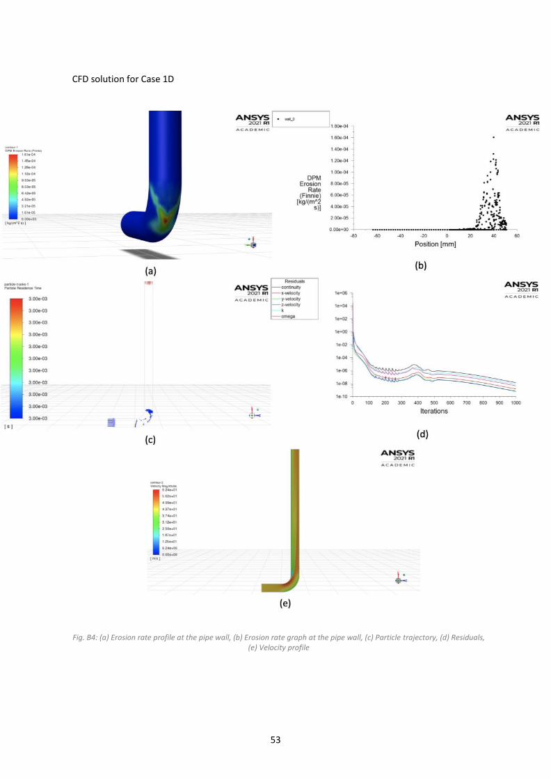
53

CFD solution for Case 1D

Fig. B4: (a) Erosion rate profile at the pipe wall, (b) Erosion rate graph at the pipe wall, (c) Particle trajectory, (d) Residuals, (e) Velocity profile

54

CFD solution for Case 1E – SST 𝑘 − 𝜔

Fig. B5: (a) Erosion rate profile at the pipe wall, (b) Erosion rate graph at the pipe wall, (c) Particle trajectory, (d) Residuals, (e) Velocity profile

55

CFD solution for Case 1E – RNG 𝑘 − 𝜀

Fig. B6: (a) Erosion rate profile at the pipe wall, (b) Erosion rate graph at the pipe wall, (c) Particle trajectory, (d) Residuals,

(e) Velocity profile

56

CFD solution for Case 1F – SST 𝑘 − 𝜔

Fig. B7: (a) Erosion rate profile at the pipe wall, (b) Erosion rate graph at the pipe wall, (c) Particle trajectory, (d) Residuals,

(e) Velocity profile

57

CFD solution for Case 1F – RNG 𝑘 − 𝜀

Fig. B8: (a) Erosion rate profile at the pipe wall, (b) Erosion rate graph at the pipe wall, (c) Particle trajectory, (d) Residuals,

(e) Velocity profile

58

CFD solution for Case 1G – SST 𝑘 − 𝜔

Fig. B9: (a) Erosion rate profile at the pipe wall, (b) Erosion rate graph at the pipe wall, (c) Particle trajectory, (d) Residuals,

(e) Velocity profile

59

CFD solution for Case 1G – RNG 𝑘 − 𝜀

Fig. B10: (a) Erosion rate profile at the pipe wall, (b) Erosion rate graph at the pipe wall, (c) Particle trajectory, (d) Residuals, (e) Velocity profile

60

CFD solution for Case 1H – SST 𝑘 − 𝜔

Fig. B11: (a) Erosion rate profile at the pipe wall, (b) Erosion rate graph at the pipe wall, (c) Particle trajectory, (d) Residuals, (e) Velocity profile

61

CFD solution for Case 1H – RNG 𝑘 − 𝜀

Fig. B12: (a) Erosion rate profile at the pipe wall, (b) Erosion rate graph at the pipe wall, (c) Particle trajectory, (d) Residuals, (e) Velocity profile

62

CFD solution for Case 1I – SST 𝑘 − 𝜔

Fig. B13: (a) Erosion rate profile at the pipe wall, (b) Erosion rate graph at the pipe wall, (c) Particle trajectory, (d) Residuals, (e) Velocity profile

63

CFD solution for Case 1I – RNG 𝑘 − 𝜀

Fig. B14: (a) Erosion rate profile at the pipe wall, (b) Erosion rate graph at the pipe wall, (c) Particle trajectory, (d) Residuals, (e) Velocity profile

64

CFD solution for Case 1J

Fig. B15: (a) Erosion rate profile at the pipe wall, (b) Erosion rate graph at the pipe wall, (c) Particle trajectory, (d) Residuals, (e) Velocity profile

65

CFD solution for Case 1K

Fig. B16: (a) Erosion rate profile at the pipe wall, (b) Erosion rate graph at the pipe wall, (c) Particle trajectory, (d) Residuals, (e) Velocity profile

66

CFD solution for Case 1L

Fig. B17: (a) Erosion rate profile at the pipe wall, (b) Erosion rate graph at the pipe wall, (c) Particle trajectory, (d) Residuals, (e) Velocity profile

67

CFD solution for Case 1M

Fig. B18: (a) Erosion rate profile at the pipe wall, (b) Erosion rate graph at the pipe wall, (c) Particle trajectory, (d) Residuals, (e) Velocity profile

68

CFD solution for Case 1N

Fig. B19: (a) Erosion rate profile at the pipe wall, (b) Erosion rate graph at the pipe wall, (c) Particle trajectory, (d) Residuals, (e) Velocity profile

69

CFD solution for Case 2A

Fig. B20: (a) Erosion rate profile at the pipe wall, (b) Erosion rate graph at the pipe wall, (c) Particle trajectory, (d) Residuals, (e) Velocity profile

70

CFD solution for Case 2B

Fig. B21: (a) Erosion rate profile at the pipe wall, (b) Erosion rate graph at the pipe wall, (c) Particle trajectory, (d) Residuals, (e) Velocity profile

71

CFD solution for Case 2C

Fig. B22: (a) Erosion rate profile at the pipe wall, (b) Erosion rate graph at the pipe wall, (c) Particle trajectory, (d) Residuals, (e) Velocity profile

72

CFD solution for Case 2D

Fig. B23: (a) Erosion rate profile at the pipe wall, (b) Erosion rate graph at the pipe wall, (c) Particle trajectory, (d) Residuals, (e) Velocity profile

73

CFD solution for Case 3A at 11 m/s

Fig. B24: (a) Erosion rate profile at the pipe wall, (b) Erosion rate graph at the pipe wall, (c) Particle trajectory, (d) Residuals, (e) Velocity profile

74

CFD solution for Case 3A at 15 m/s

Fig. B25: (a) Erosion rate profile at the pipe wall, (b) Erosion rate graph at the pipe wall, (c) Particle trajectory, (d) Residuals, (e) Velocity profile

75

CFD solution for Case 3A at 23 m/s

Fig. B26: (a) Erosion rate profile at the pipe wall, (b) Erosion rate graph at the pipe wall, (c) Particle trajectory, (d) Residuals, (e) Velocity profile

76

CFD solution for Case 3A at 27 m/s

Fig. B27: (a) Erosion rate profile at the pipe wall, (b) Erosion rate graph at the pipe wall, (c) Particle trajectory, (d) Residuals, (e) Velocity profile

77

CFD solution for Case 3B at 11 m/s

Fig. B28: (a) Erosion rate profile at the pipe wall, (b) Erosion rate graph at the pipe wall, (c) Particle trajectory, (d) Residuals, (e) Velocity profile

78

CFD solution for Case 3B at 15 m/s

Fig. B29: (a) Erosion rate profile at the pipe wall, (b) Erosion rate graph at the pipe wall, (c) Particle trajectory, (d) Residuals, (e) Velocity profile

79

CFD solution for Case 3B at 23 m/s

Fig. B30: (a) Erosion rate profile at the pipe wall, (b) Erosion rate graph at the pipe wall, (c) Particle trajectory, (d) Residuals, (e) Velocity profile

80

CFD solution for Case 3B at 27 m/s

Fig. B31: (a) Erosion rate profile at the pipe wall, (b) Erosion rate graph at the pipe wall, (c) Particle trajectory, (d) Residuals, (e) Velocity profile

81

CFD solution for Case 3C at 11 m/s

Fig. B32: (a) Erosion rate profile at the pipe wall, (b) Erosion rate graph at the pipe wall, (c) Particle trajectory, (d) Residuals, (e) Velocity profile

82

CFD solution for Case 3C at 15 m/s

Fig. B33: (a) Erosion rate profile at the pipe wall, (b) Erosion rate graph at the pipe wall, (c) Particle trajectory, (d) Residuals, (e) Velocity profile

83

CFD solution for Case 3C at 23 m/s

Fig. B34: (a) Erosion rate profile at the pipe wall, (b) Erosion rate graph at the pipe wall, (c) Particle trajectory, (d) Residuals, (e) Velocity profile

84

CFD solution for Case 3C at 27 m/s

Fig. B35: (a) Erosion rate profile at the pipe wall, (b) Erosion rate graph at the pipe wall, (c) Particle trajectory, (d) Residuals, (e) Velocity profile

85

CFD solution for Case 3D at 11 m/s

Fig. B36: (a) Erosion rate profile at the pipe wall, (b) Erosion rate graph at the pipe wall, (c) Particle trajectory, (d) Residuals, (e) Velocity profile

86

CFD solution for Case 3D at 15 m/s

Fig. B37: (a) Erosion rate profile at the pipe wall, (b) Erosion rate graph at the pipe wall, (c) Particle trajectory, (d) Residuals, (e) Velocity profile

87

CFD solution for Case 3D at 23 m/s

Fig. B38: (a) Erosion rate profile at the pipe wall, (b) Erosion rate graph at the pipe wall, (c) Particle trajectory, (d) Residuals, (e) Velocity profile

88

CFD solution for Case 3D at 27 m/s

Fig. B39: (a) Erosion rate profile at the pipe wall, (b) Erosion rate graph at the pipe wall, (c) Particle trajectory, (d) Residuals, (e) Velocity profile