T-test · T-test A t-test is a hypothesis test in which the test statistic follows a Student’s...
19
T-test A t-test is a hypothesis test in which the test statistic follows a Student’s t-distribution under the null hypothesis. There are several different test statistics that fall into the category of a t-test. One-Sample t-test 0 1 x t s n df n Independent Two-Sample t-test 1 2 1 2 1 2 1 2 2 2 2 1 2 2 2 xx xx x x x x t s n s s s df n Unequal Sample Size Two-Sample t-test 1 2 1 2 1 2 1 2 1 2 2 2 1 2 1 2 1 2 1 1 1 1 2 2 xx x x xx x x t s n n n s n s s n n df n n Unequal Sample Size and Unequal Variance Two-Sample t-test
Transcript of T-test · T-test A t-test is a hypothesis test in which the test statistic follows a Student’s...
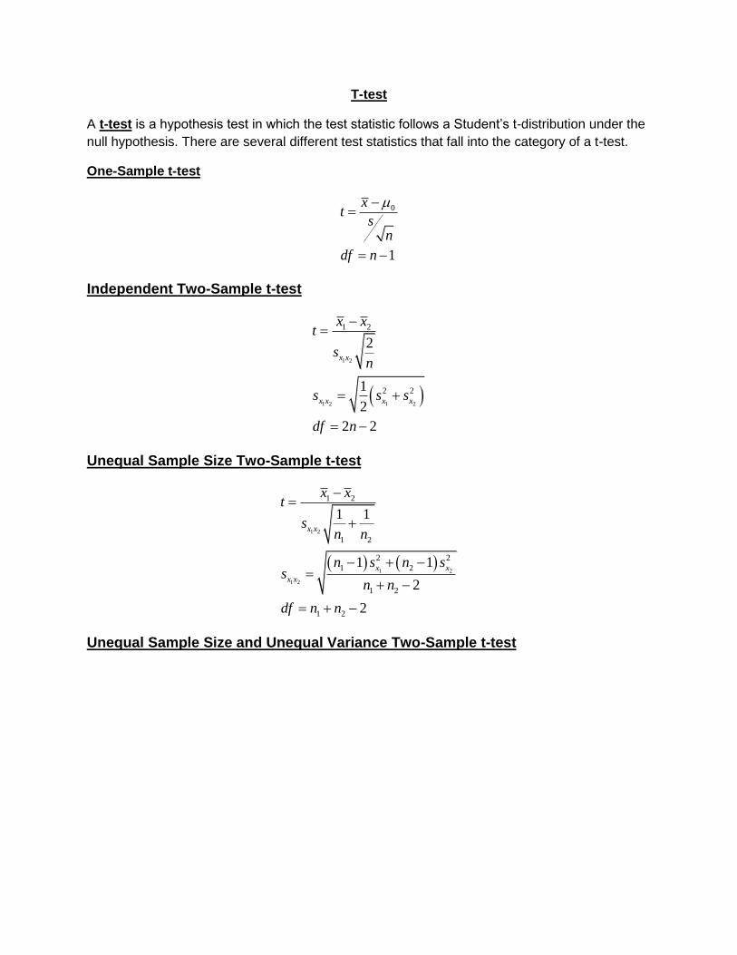
T-test
A t-test is a hypothesis test in which the test statistic follows a Student’s t-distribution under the
null hypothesis. There are several different test statistics that fall into the category of a t-test.
One-Sample t-test
0
1
xt
sn
df n
Independent Two-Sample t-test
1 2
1 2 1 2
1 2
2 2
2
1
2
2 2
x x
x x x x
x xt
sn
s s s
df n
Unequal Sample Size Two-Sample t-test
1 2
1 2
1 2
1 2
1 2
2 2
1 2
1 2
1 2
1 1
1 1
2
2
x x
x x
x x
x xt
sn n
n s n ss
n n
df n n
Unequal Sample Size and Unequal Variance Two-Sample t-test
1 2
1 2
1 2
2 2
1 2
1 2
22 2
1 2
1 2
2 22 2
1 2
1 2
1 21 1
x x
x x
x xt
s
s ss
n n
s s
n ndf
s s
n n
n n
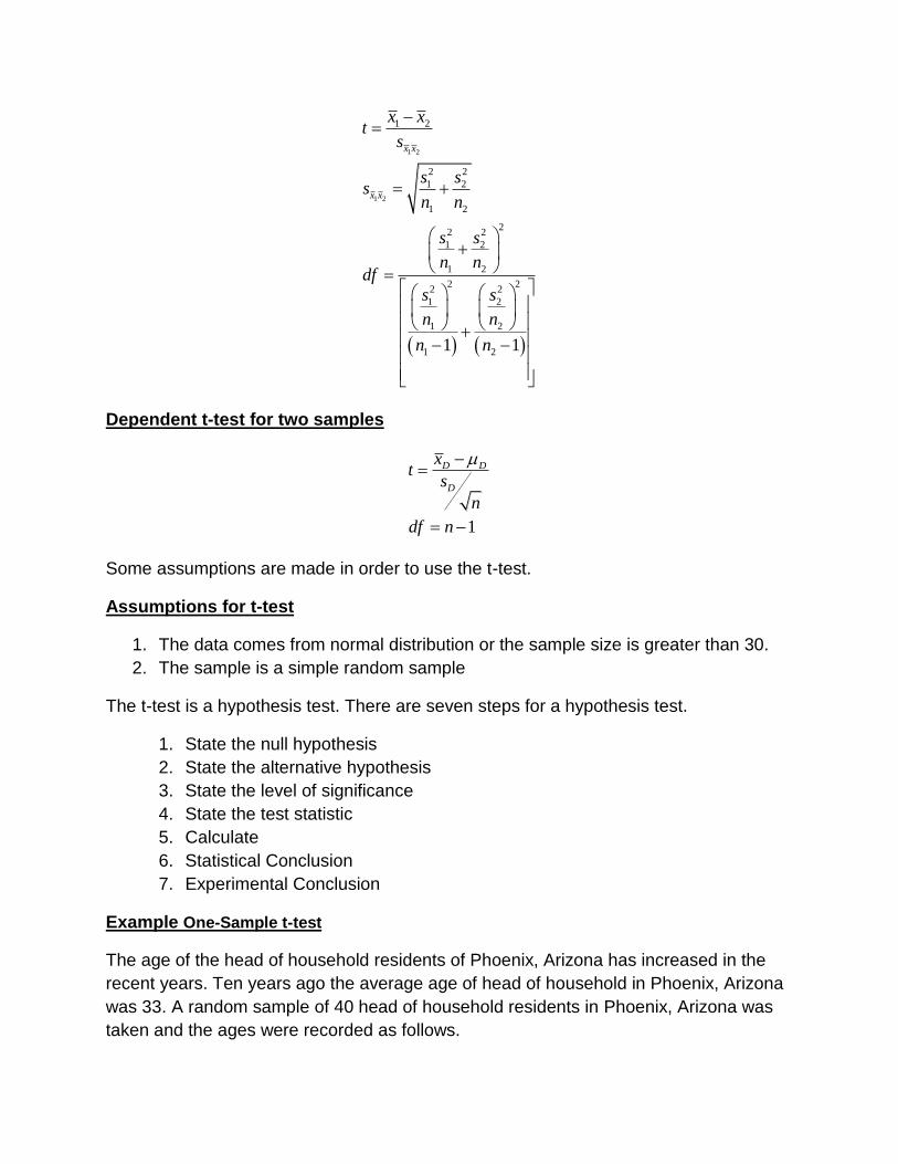
Dependent t-test for two samples
1
D D
D
xt
s
n
df n
Some assumptions are made in order to use the t-test.
Assumptions for t-test
1. The data comes from normal distribution or the sample size is greater than 30.
2. The sample is a simple random sample
The t-test is a hypothesis test. There are seven steps for a hypothesis test.
1. State the null hypothesis
2. State the alternative hypothesis
3. State the level of significance
4. State the test statistic
5. Calculate
6. Statistical Conclusion
7. Experimental Conclusion
Example One-Sample t-test
The age of the head of household residents of Phoenix, Arizona has increased in the
recent years. Ten years ago the average age of head of household in Phoenix, Arizona
was 33. A random sample of 40 head of household residents in Phoenix, Arizona was
taken and the ages were recorded as follows.
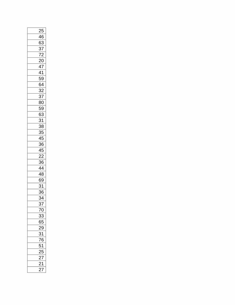
25
46
63
37
72
20
47
41
59
64
32
37
80
59
63
31
38
35
45
36
45
22
36
44
48
69
31
36
34
37
70
33
65
29
31
76
51
25
27
21
27
We wish to use this data to test if the hypothesis that the average age of head of
household residents in Phoenix, Arizona has increased.
This is a hypothesis test so we will need to go through the seven steps of a hypothesis
testing.
Step 1: Null Hypothesis
Since in the past the mean Head of Household age was 33 that is the statement of no
effect which is what the null hypothesis gives.
0 : 33H
Step 2: Alternative Hypothesis
We want to know if the mean head of household age has increased so the alternative is
: 33AH
This is a one-tailed test as we are only looking at a one-sided alternative.
Step 3: Level of Significance
0.05
Step 4: Test Statistic
The test statistic needed is for a one-sample t-test. It is one-sample because we are
only looking at one set of data values. The other requirements for a t-test have been
met as the sample size is 40 > 30 and the sample is a simple random sample.
0
1
xt
sn
df n
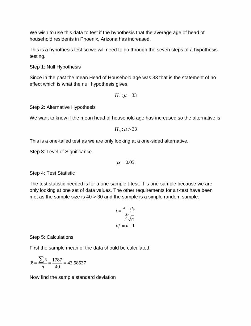
Step 5: Calculations
First the sample mean of the data should be calculated.
178743.58537
40
xx
n
Now find the sample standard deviation
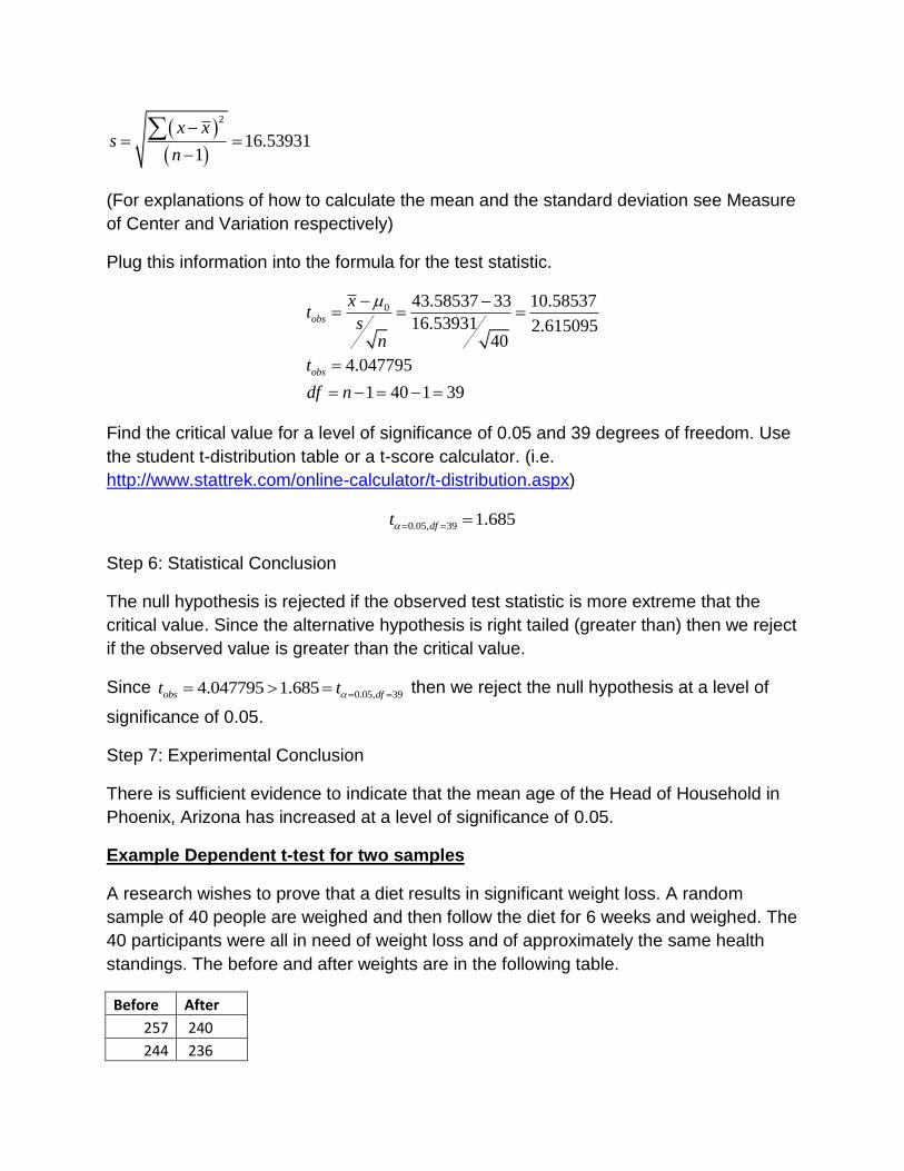
2
16.539311
x xs
n
(For explanations of how to calculate the mean and the standard deviation see Measure
of Center and Variation respectively)
Plug this information into the formula for the test statistic.
0 43.58537 33 10.58537
16.53931 2.61509540
4.047795
1 40 1 39
obs
obs
xt
sn
t
df n
Find the critical value for a level of significance of 0.05 and 39 degrees of freedom. Use
the student t-distribution table or a t-score calculator. (i.e.
http://www.stattrek.com/online-calculator/t-distribution.aspx)
0.05, 39 1.685dft
Step 6: Statistical Conclusion
The null hypothesis is rejected if the observed test statistic is more extreme that the
critical value. Since the alternative hypothesis is right tailed (greater than) then we reject
if the observed value is greater than the critical value.
Since 0.05, 394.047795 1.685obs dft t then we reject the null hypothesis at a level of
significance of 0.05.
Step 7: Experimental Conclusion
There is sufficient evidence to indicate that the mean age of the Head of Household in
Phoenix, Arizona has increased at a level of significance of 0.05.
Example Dependent t-test for two samples
A research wishes to prove that a diet results in significant weight loss. A random
sample of 40 people are weighed and then follow the diet for 6 weeks and weighed. The
40 participants were all in need of weight loss and of approximately the same health
standings. The before and after weights are in the following table.
Before After
257 240
244 236

151 145
229 200
151 146
296 277
151 147
219 201
265 215
177 160
202 190
194 172
198 180
175 170
194 183
281 233
148 240
260 200
159 250
176 267
255 202
212 195
287 243
242 204
248 205
224 199
185 164
210 173
157 150
170 152
293 232
152 140
263 202
154 142
287 260
249 195
161 153
244 204
267 207
300 245
300 234
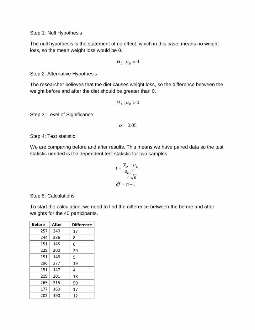
Step 1: Null Hypothesis
The null hypothesis is the statement of no effect, which in this case, means no weight
loss, so the mean weight loss would be 0.
0 : 0DH
Step 2: Alternative Hypothesis
The researcher believes that the diet causes weight loss, so the difference between the
weight before and after the diet should be greater than 0.
: 0A DH
Step 3: Level of Significance
0.05
Step 4: Test statistic
We are comparing before and after results. This means we have paired data so the test
statistic needed is the dependent test statistic for two samples.
1
D D
D
xt
s
n
df n
Step 5: Calculations
To start the calculation, we need to find the difference between the before and after
weights for the 40 participants.
Before After Difference
257 240 17
244 236 8
151 145 6
229 200 29
151 146 5
296 277 19
151 147 4
219 201 18
265 215 50
177 160 17
202 190 12
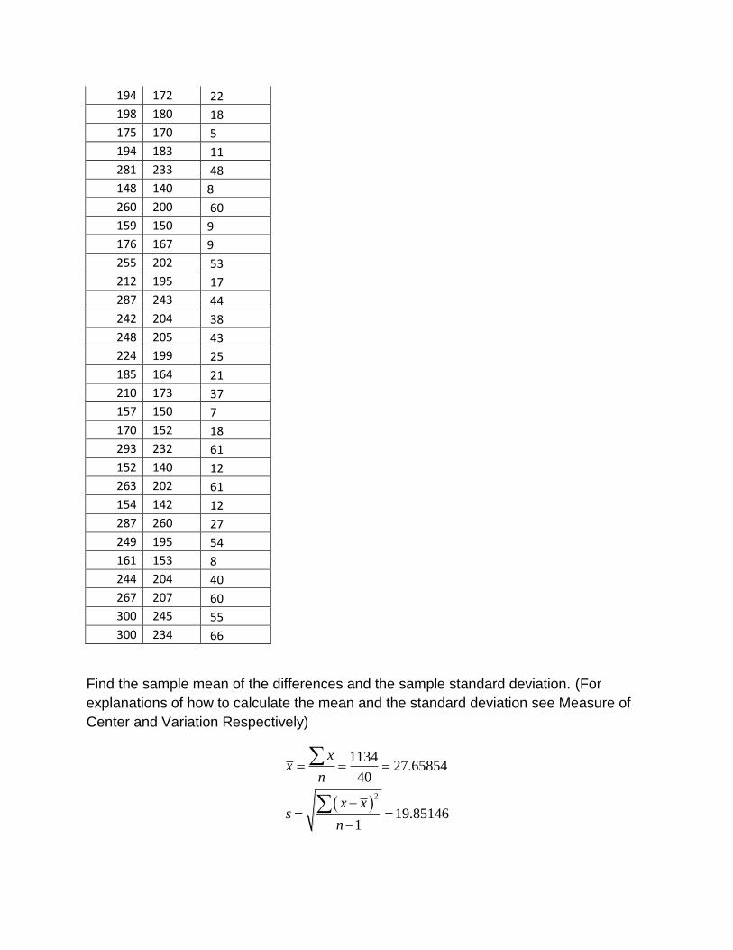
194 172 22
198 180 18
175 170 5
194 183 11
281 233 48
148 140 8
260 200 60
159 150 9
176 167 9
255 202 53
212 195 17
287 243 44
242 204 38
248 205 43
224 199 25
185 164 21
210 173 37
157 150 7
170 152 18
293 232 61
152 140 12
263 202 61
154 142 12
287 260 27
249 195 54
161 153 8
244 204 40
267 207 60
300 245 55
300 234 66
Find the sample mean of the differences and the sample standard deviation. (For
explanations of how to calculate the mean and the standard deviation see Measure of
Center and Variation Respectively)
2
113427.65854
40
19.851461
xx
n
x xs
n
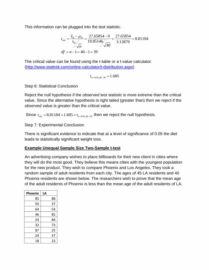
This information can be plugged into the test statistic.
27.65854 0 27.658548.81184
19.85146 3.1387940
1 40 1 39
D Dobs
D
xt
s
n
df n
The critical value can be found using the t-table or a t-value calculator.
(http://www.stattrek.com/online-calculator/t-distribution.aspx)
0.05, 39 1.685dft
Step 6: Statistical Conclusion
Reject the null hypothesis if the observed test statistic is more extreme than the critical
value. Since the alternative hypothesis is right tailed (greater than) then we reject if the
observed value is greater than the critical value.
Since 0.05, 398.81184 1.685obs dft t then we reject the null hypothesis.
Step 7: Experimental Conclusion
There is significant evidence to indicate that at a level of significance of 0.05 the diet
leads to statistically significant weight loss.
Example Unequal Sample Size Two-Sample t-test
An advertising company wishes to place billboards for their new client in cities where
they will do the most good. They believe this means cities with the youngest population
for the new product. They wish to compare Phoenix and Los Angeles. They took a
random sample of adult residents from each city. The ages of 45 LA residents and 40
Phoenix residents are shown below. The researchers wish to prove that the mean age
of the adult residents of Phoenix is less than the mean age of the adult residents of LA.
Phoenix LA
85 88
50 37
64 54
46 85
24 84
32 73
87 25
24 37
18 23
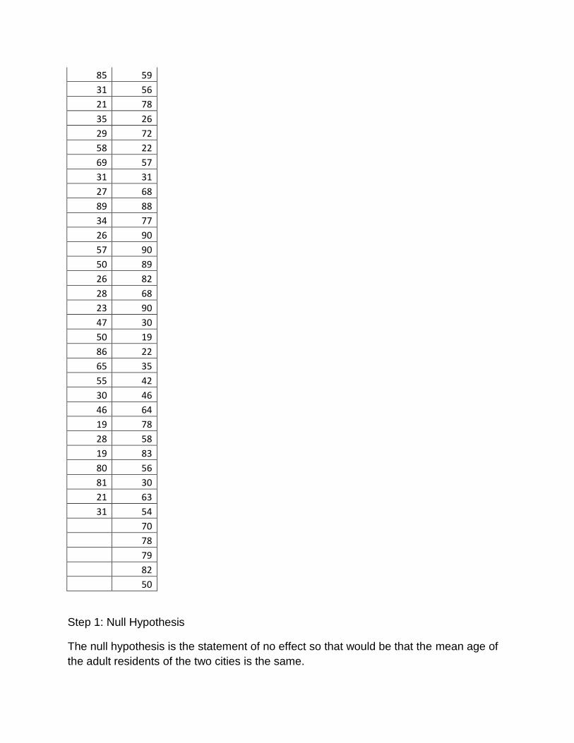
85 59
31 56
21 78
35 26
29 72
58 22
69 57
31 31
27 68
89 88
34 77
26 90
57 90
50 89
26 82
28 68
23 90
47 30
50 19
86 22
65 35
55 42
30 46
46 64
19 78
28 58
19 83
80 56
81 30
21 63
31 54
70
78
79
82
50
Step 1: Null Hypothesis
The null hypothesis is the statement of no effect so that would be that the mean age of
the adult residents of the two cities is the same.
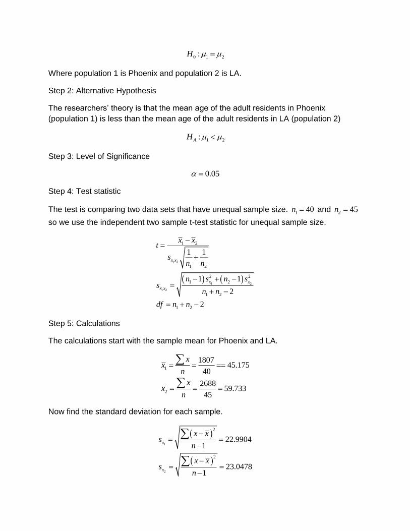
0 1 2:H
Where population 1 is Phoenix and population 2 is LA.
Step 2: Alternative Hypothesis
The researchers’ theory is that the mean age of the adult residents in Phoenix
(population 1) is less than the mean age of the adult residents in LA (population 2)
1 2:AH
Step 3: Level of Significance
0.05
Step 4: Test statistic
The test is comparing two data sets that have unequal sample size. 1 40n and 2 45n
so we use the independent two sample t-test statistic for unequal sample size.
1 2
1 2
1 2
1 2
1 2
2 2
1 2
1 2
1 2
1 1
1 1
2
2
x x
x x
x x
x xt
sn n
n s n ss
n n
df n n
Step 5: Calculations
The calculations start with the sample mean for Phoenix and LA.
1
2
180745.175
40
268859.733
45
xx
n
xx
n
Now find the standard deviation for each sample.
1
2
2
2
22.99041
23.04781
x
x
x xs
n
x xs
n
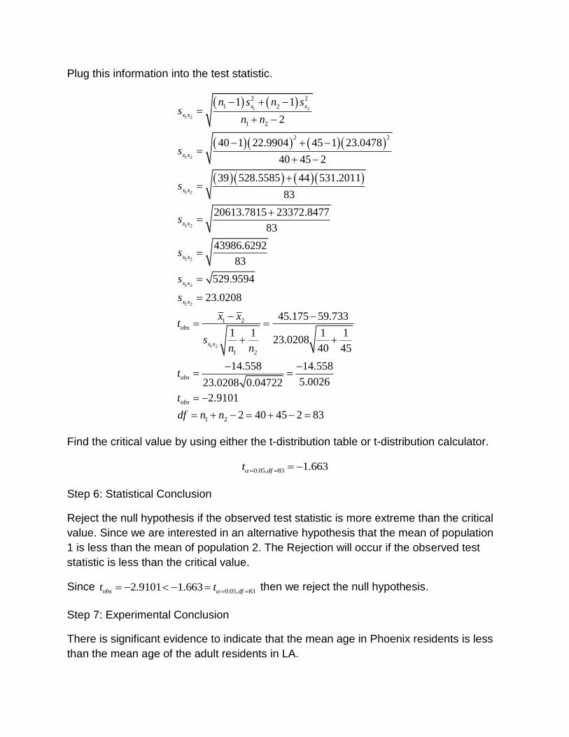
Plug this information into the test statistic.
1 2
1 2
1 2
1 2
1 2
1 2
1 2
1 2
1 2
2 2
1 2
1 2
2 2
1 2
1 2
1 1
2
40 1 22.9904 45 1 23.0478
40 45 2
39 528.5585 44 531.2011
83
20613.7815 23372.8477
83
43986.6292
83
529.9594
23.0208
45.175
1 1
x x
x x
x x
x x
x x
x x
x x
x x
obs
x x
n s n ss
n n
s
s
s
s
s
s
x xt
sn n
1 2
59.733
1 123.0208
40 45
14.558 14.558
5.002623.0208 0.04722
2.9101
2 40 45 2 83
obs
obs
t
t
df n n
Find the critical value by using either the t-distribution table or t-distribution calculator.
0.05, 83 1.663dft
Step 6: Statistical Conclusion
Reject the null hypothesis if the observed test statistic is more extreme than the critical
value. Since we are interested in an alternative hypothesis that the mean of population
1 is less than the mean of population 2. The Rejection will occur if the observed test
statistic is less than the critical value.
Since 0.05, 832.9101 1.663obs dft t then we reject the null hypothesis.
Step 7: Experimental Conclusion
There is significant evidence to indicate that the mean age in Phoenix residents is less
than the mean age of the adult residents in LA.
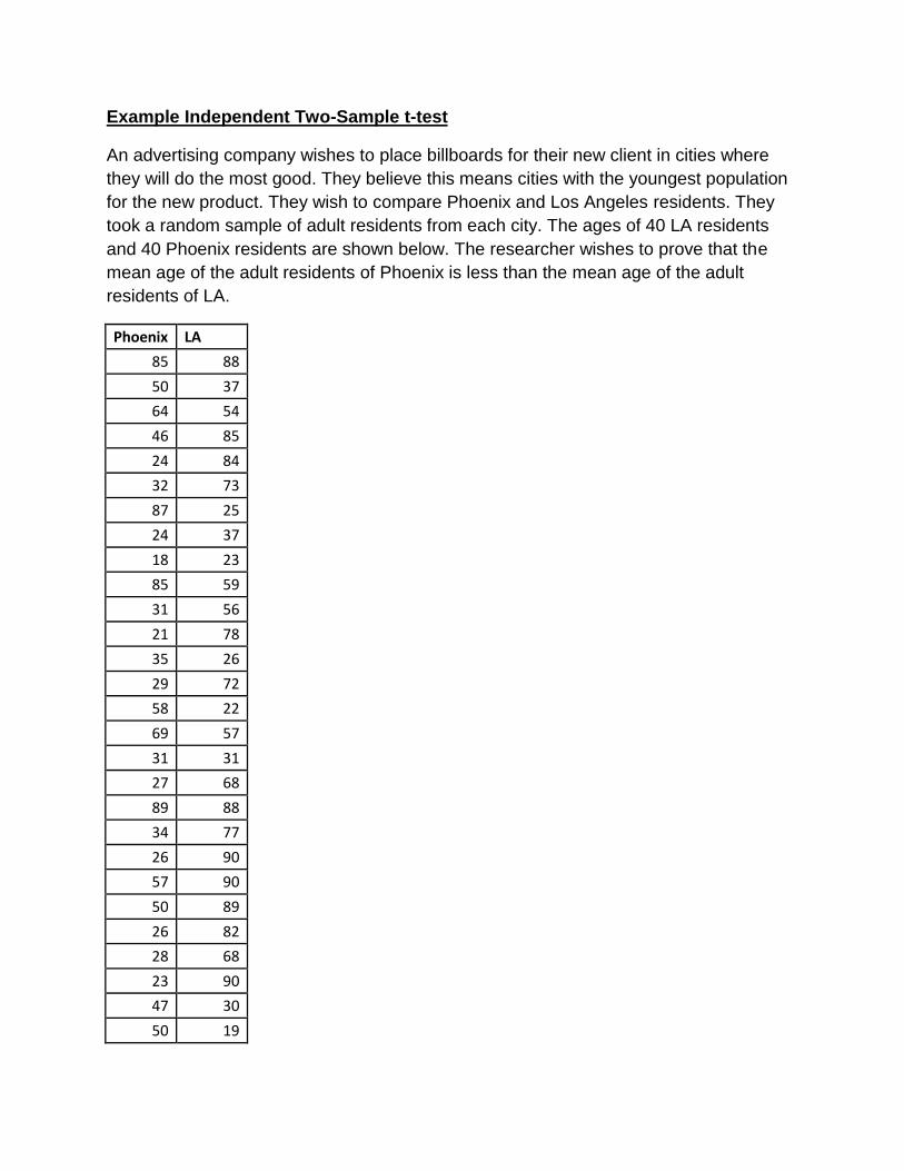
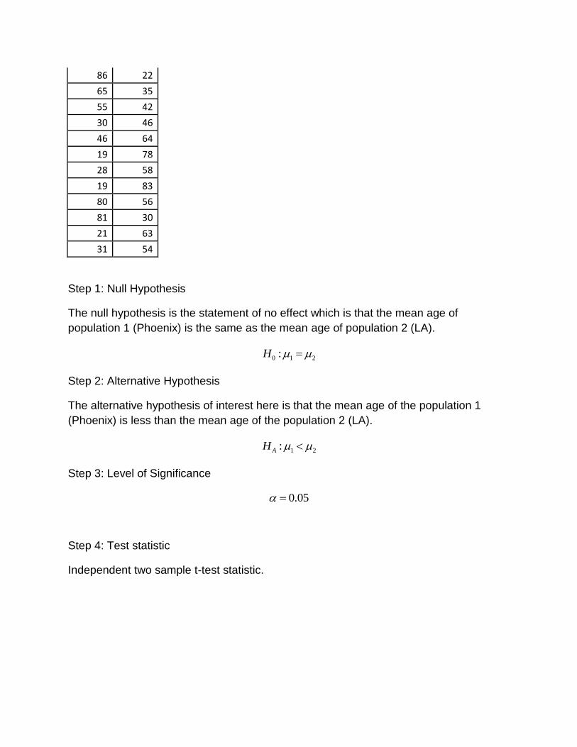
Example Independent Two-Sample t-test
An advertising company wishes to place billboards for their new client in cities where
they will do the most good. They believe this means cities with the youngest population
for the new product. They wish to compare Phoenix and Los Angeles residents. They
took a random sample of adult residents from each city. The ages of 40 LA residents
and 40 Phoenix residents are shown below. The researcher wishes to prove that the
mean age of the adult residents of Phoenix is less than the mean age of the adult
residents of LA.
Phoenix LA
85 88
50 37
64 54
46 85
24 84
32 73
87 25
24 37
18 23
85 59
31 56
21 78
35 26
29 72
58 22
69 57
31 31
27 68
89 88
34 77
26 90
57 90
50 89
26 82
28 68
23 90
47 30
50 19
86 22
65 35
55 42
30 46
46 64
19 78
28 58
19 83
80 56
81 30
21 63
31 54
Step 1: Null Hypothesis
The null hypothesis is the statement of no effect which is that the mean age of
population 1 (Phoenix) is the same as the mean age of population 2 (LA).
0 1 2:H
Step 2: Alternative Hypothesis
The alternative hypothesis of interest here is that the mean age of the population 1
(Phoenix) is less than the mean age of the population 2 (LA).
1 2:AH
Step 3: Level of Significance
0.05
Step 4: Test statistic
Independent two sample t-test statistic.
1 2
1 2 1 2
1 2
2 2
2
1
2
2 2
x x
x x x x
x xt
sn
s s s
df n
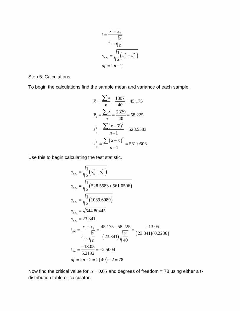
Step 5: Calculations
To begin the calculations find the sample mean and variance of each sample.
1
2
1
2
2
2
2
2
180745.175
40
232958.225
40
528.55831
561.05061
x
x
xx
n
xx
n
x xs
n
x xs
n
Use this to begin calculating the test statistic.
1 2 1 2
1 2
1 2
1 2
1 2
1 2
2 2
1 2
1
2
1528.5583 561.0506
2
11089.6089
2
544.80445
23.341
45.175 58.225 13.05
23.341 0.22362 223.341
40
13.052.5004
5.2192
2 2 2 40 2 78
x x x x
x x
x x
x x
x x
obs
x x
obs
s s s
s
s
s
s
x xt
sn
t
df n
Now find the critical value for 0.05 and degrees of freedom = 78 using either a t-
distribution table or calculator.
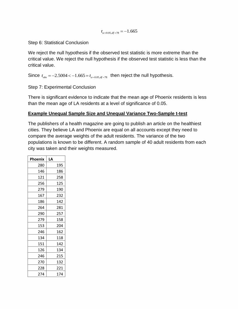
0.05, 78 1.665dft
Step 6: Statistical Conclusion
We reject the null hypothesis if the observed test statistic is more extreme than the
critical value. We reject the null hypothesis if the observed test statistic is less than the
critical value.
Since 0.05, 782.5004 1.665obs dft t then reject the null hypothesis.
Step 7: Experimental Conclusion
There is significant evidence to indicate that the mean age of Phoenix residents is less
than the mean age of LA residents at a level of significance of 0.05.
Example Unequal Sample Size and Unequal Variance Two-Sample t-test
The publishers of a health magazine are going to publish an article on the healthiest
cities. They believe LA and Phoenix are equal on all accounts except they need to
compare the average weights of the adult residents. The variance of the two
populations is known to be different. A random sample of 40 adult residents from each
city was taken and their weights measured.
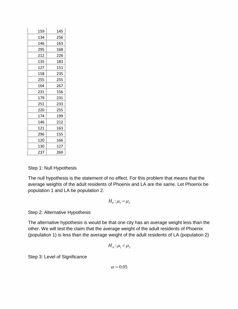
Phoenix LA
280 195
146 186
121 258
256 125
279 190
167 232
186 142
264 281
290 257
279 158
153 204
246 162
134 118
151 142
126 134
246 215
270 132
228 221
274 174
159 145
134 256
146 163
295 168
212 226
135 183
127 151
158 235
255 255
164 267
231 156
179 231
251 233
220 255
174 199
146 212
121 163
296 155
120 166
130 127
237 269
Step 1: Null Hypothesis
The null hypothesis is the statement of no effect. For this problem that means that the
average weights of the adult residents of Phoenix and LA are the same. Let Phoenix be
population 1 and LA be population 2.
0 1 2:H
Step 2: Alternative Hypothesis
The alternative hypothesis is would be that one city has an average weight less than the
other. We will test the claim that the average weight of the adult residents of Phoenix
(population 1) is less than the average weight of the adult residents of LA (population 2)
1 2:AH
Step 3: Level of Significance
0.05
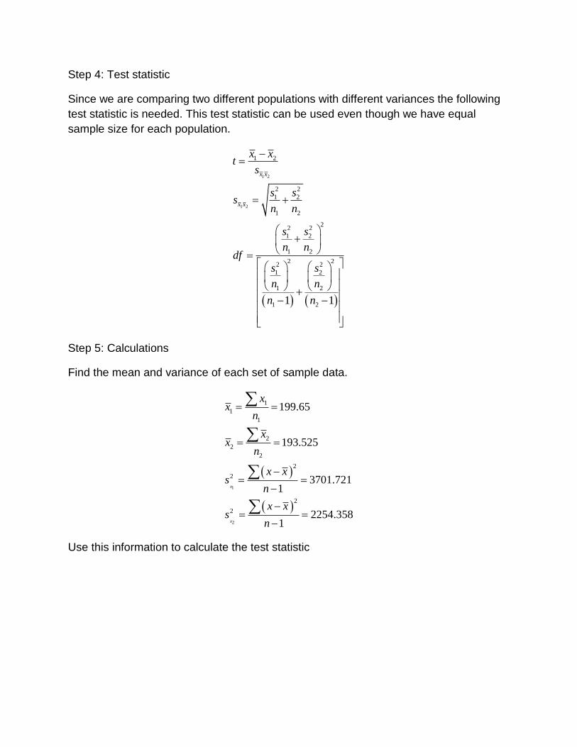
Step 4: Test statistic
Since we are comparing two different populations with different variances the following
test statistic is needed. This test statistic can be used even though we have equal
sample size for each population.
1 2
1 2
1 2
2 2
1 2
1 2
22 2
1 2
1 2
2 22 2
1 2
1 2
1 21 1
x x
x x
x xt
s
s ss
n n
s s
n ndf
s s
n n
n n
Step 5: Calculations
Find the mean and variance of each set of sample data.
1
2
1
1
1
2
2
2
2
2
2
2
199.65
193.525
3701.7211
2254.3581
x
x
xx
n
xx
n
x xs
n
x xs
n
Use this information to calculate the test statistic
1 2
1 2
1 2
1 2
2 2
1 2
1 2
1 2
22 2
1 2
1 2
2 22 2
1 2
1 2
1 2
3701.721 2254.358
40 40
92.5401 56.3589 148.8991
12.2024
199.65 193.525 6.125
12.2024 12.2024
0.5020
1 1
x x
x x
x x
obs
x x
obs
s ss
n n
s
s
x xt
s
t
s s
n ndf
s s
n n
n n
2
2 2
2
3701.721 2254.358
40 40
3701.721 2254.358
40 40
40 1 40 1
148.9019 22171.798273.6508 74
219.5952 81.4444 301.0396df
Find the critical value for the t-distribution with alpha=0.05 and degrees of freedom of
74. Use either a table or a t-distribution calculator available on the web.
0.05, 74 1.666dft
Step 6: Statistical Conclusion
Reject the null hypothesis if the observed test statistic is more extreme than the critical
value. Since we are looking at a left tailed alternative hypothesis that we reject the null
hypothesis if the observed test statistic is less than the critical value.
Since 0.05, 740.5020 1.666obs dft t then we fail to reject the null hypothesis.
Step 7: Experimental Conclusion
There is not sufficient evidence to indicate that the mean weight of Phoenix is different
than the mean weight of LA at a level of significance of 0.05.