Kellner_1999-Software Process Simulation Modeling - Why What How

SYSTEMS ENGINEERING PROCESS MODELING AND SIMULATION
A THESIS SUBMITTED TO THE GRADUATE SCHOOL OF NATURAL AND APPLIED SCIENCES
OF MIDDLE EAST TECHNICAL UNIVERSITY
BY
MERVE ARIKAN
IN PARTIAL FULFILLMENT OF THE REQUIREMENTS FOR
THE DEGREE OF MASTER OF SCIENCE IN
INDUSTRIAL ENGINEERING
SEPTEMBER 2012
Approval of the thesis:
SYSTEMS ENGINEERING PROCESS MODELING AND SIMULATION
submitted by MERVE ARIKAN in partial fulfillment of the requirements for the degree of Master of Science in Industrial Engineering Department, Middle East Technical University by,
Prof. Dr. Canan Özgen Dean, Graduate School of Natural and Applied Sciences Prof. Dr. Sinan Kayalıgil Head of Department, Industrial Engineering Prof. Dr. Nur Evin Özdemirel Supervisor, Industrial Engineering Dept., METU
Examining Committee Members:
Prof. Dr. Gülser Köksal Industrial Engineering Dept., METU Prof. Dr. Nur Evin Özdemirel Industrial Engineering Dept., METU Prof. Dr. Ömer Kırca Industrial Engineering Dept., METU Assistant Prof. Dr. Özgen Karaer Industrial Engineering Dept., METU Ömer Faruk Kırcalı, M.Sc. Systems Engineering Chief, TAI Date: 13.09.2012

iii
I hereby declare that all information in this document has been obtained and presented in accordance with academic rules and ethical conduct. I also declare that, as required by these rules and conduct, I have fully cited and referenced all material and results that are not original to this work.
Name, Last name : Merve Arıkan
Signature :

iv
ABSTRACT
SYSTEMS ENGINEERING PROCESS MODELING AND SIMULATION
Arıkan, Merve
M.Sc., Department of Industrial Engineering
Supervisor: Prof. Dr. Nur Evin Özdemirel
September 2012, 132 pages
In this study, an approach is proposed to model and simulate the systems
engineering process of design projects. One of the main aims is to model the
systems engineering process, treating the process itself as a complex system. A
conceptual model is developed as a result of a two-phase survey conducted with
systems engineers. The conceptual model includes two levels of activity networks.
Each first level systems engineering activity has its own network of second level
activities. The model is then implemented in object-oriented modeling language,
namely SysML, using block definition diagrams and activity diagrams. Another
aim is to generate a discrete event simulation model of the process for performance
evaluation. For this purpose the SysML model is transformed to an Arena model
using an Excel interface and VBA codes. Three deterministic and three stochastic
cases are created to represent systems engineering process alternatives, which
originate from the same conceptual model but possess different activity durations,
resource availabilities and resource requirements. The scale of the project and the
effect of uncertainty in activity durations are also considered. The proposed
approach is applied to each of these six cases, developing the SysML models,
transforming them to Arena models, and running the simulations. Project duration
and resource utilization results are reported for these cases.
Keywords: Systems Engineering, Object-oriented Modeling, SysML, Discrete
Event Simulation, Arena

v
ÖZ
SİSTEM MÜHENDİSLİĞİ SÜRECİNİN MODELLENMESİ VE SİMÜLASYONU
Arıkan, Merve
Yüksek Lisans, Endüstri Mühendisliği Bölümü
Tez Yöneticisi: Prof. Dr. Nur Evin Özdemirel
Eylül 2012, 132 sayfa
Bu çalışmada tasarım projelerine ait sistem mühendisliği sürecinin modellenmesi
ve simülasyonuna yönelik bir yöntem önerilmektedir. Temel amaçlardan biri,
sürecin kendisini karmaşık bir sistem olarak ele alarak sistem mühendisliği
sürecini modellemektir. Sistem mühendisleri ile gerçekleştirilen iki aşamalı anket
çalışmasının sonucunda bir kavramsal model elde edilmiştir. Kavramsal model, iki
seviye aktivite ağı içermektedir. Her bir birinci seviye sistem mühendisliği
aktivitesi, kendine ait ikinci seviye aktivite ağına sahiptir. Daha sonra model,
nesne yönelimli modelleme dilinde, SysML üzerinde, blok tanımlama
diyagramları ve aktivite diyagramları kullanılarak uygulamaya geçirilmiştir. Diğer
bir amaç ise performans değerlendirmesi için sürecin ayrık olay simülasyon
modelini oluşturmaktır. Bu amaçla, Excel ara yüzü ve VBA kodları kullanılarak
SysML modeli bir Arena modeline dönüştürülmüştür. Aynı kavramsal modelden
gelen fakat farklı aktivite süreleri, kaynak miktarları ve kaynak gereksinimlerine
sahip olan sistem mühendisliği süreç alternatiflerini temsil etmek üzere üç
deterministik ve üç stokastik durum oluşturulmuştur. Projenin büyüklüğü ve
aktivite sürelerindeki belirsizliğin etkileri de dikkate alınmıştır. Önerilen yaklaşım,
SysML modelleri oluşturmak, bu modelleri Arena modellerine dönüştürmek ve
simülasyonlar gerçekleştirmek yoluyla altı durumdan her birine uygulanmıştır. Bu
durumlar için proje süresi ve kaynak kullanımı sonuçları raporlanmıştır.
Anahtar Kelimeler: Sistem Mühendisliği, Nesne Yönelimli Modelleme, SysML,
Ayrık Olay Simülasyonu, Arena

vi
To My Family

vii
ACKNOWLEDGEMENTS
I would like to express my deepest gratitude to my supervisor Prof. Dr. Nur Evin
Özdemirel for her insight, guidance, support and advice throughout the research.
Without her wide perspective, continuous encouragement and deep knowledge, I
would not be able to cover this relatively new subject in my thesis study. Having
the opportunity to work with Prof. Dr. Nur Evin Özdemirel is a lifetime gain to
me.
I offer sincere thanks to all of my colleagues in Systems Engineering team of
Helicopter Group in TAI for being involved in the survey studies and sharing their
experience and knowledge anytime I needed. I am privileged to experience such a
collaboration and support. I owe a great debt of gratitude to Ömer Faruk Kırcalı
for never hesitating to share his invaluable knowledge in systems engineering and
for providing means to develop my own experience by enriching my ideas and
honoring my effort.
I would also like to thank Ziya Çiftçi for introducing the world of systems
engineering to me. I will always be grateful to him for supporting me in my
decision for graduate studies and for his encouragement and understanding.
This thesis would not have been possible without the endless love and support of
my mother, my father and my two brothers. They are the main sources of
motivation for me to achieve new things in life.

viii
TABLE OF CONTENTS
ABSTRACT ........................................................................................................ iv
ÖZ ........................................................................................................................ v
ACKNOWLEDGEMENTS ................................................................................vii
TABLE OF CONTENTS .................................................................................. viii
LIST OF TABLES ................................................................................................ x
LIST OF FIGURES ............................................................................................. xi
CHAPTERS
1 INTRODUCTION ............................................................................................. 1
2 LITERATURE REVIEW ................................................................................... 5
2.1 SYSTEMS ENGINEERING CONCEPT ................................................ 5
2.2 OBJECT-ORIENTED MODELING, UML AND SysML ....................... 9
2.3 MODEL TRANSFORMATION FOR SIMULATION PURPOSES ...... 11
3 CONCEPTUAL MODEL FORMATION ......................................................... 19
3.1 CONCEPTUAL MODEL INITIALIZATION ....................................... 19
3.1.1 Systems Engineering Process as a System ...................................... 19
3.1.2 Conceptual Model Basis ................................................................ 20
3.2 THE SURVEY STUDY ........................................................................ 21
3.2.1 Survey Study – Phase 1 .................................................................. 22
3.2.2 Survey Study – Phase 1 Results ..................................................... 24
3.2.3 Survey Study – Phase 2 .................................................................. 31
3.2.4 Survey Study – Phase 2 Results ..................................................... 33
3.3 THE CONCEPTUAL MODEL ............................................................. 38
4 MODELING OF SYSTEMS ENGINEERING PROCESS IN SYSML ............ 41
4.1 MODELING STRUCTURE AND BEHAVIOR OF THE SYSTEM ..... 41
4.1.1 Modeling Structure by Block Definition Diagrams ......................... 41
4.1.2 Modeling Behavior by Activity Diagrams ...................................... 43
4.2 MANAGING MODEL PROPERTIES AND INPUT PARAMETERS .. 47

ix
5 MODEL TRANSFORMATION FOR SIMULATION ..................................... 51
5.1 BASE ARENA MODEL ....................................................................... 51
5.2 MODEL TRANSFORMATION ........................................................... 54
6 VERIFICATION CASE STUDIES AND RESULTS ....................................... 57
6.1 CASE STUDIES ................................................................................... 57
6.2 CASE STUDY RESULTS .................................................................... 60
7 CONCLUSIONS .............................................................................................. 67
REFERENCES ................................................................................................... 73
APPENDICES
A. QUESTIONNAIRE SURVEY STUDIES ....................................................... 76
A.1 QUESTIONNAIRE SURVEY STUDY – PHASE 1 ................................. 76
A.2 QUESTIONNAIRE SURVEY STUDY – PHASE 2 ................................. 80
B. SURVEY STUDY RESULTS ........................................................................ 89
C. SECOND LEVEL ACTIVITY NETWORKS ............................................... 112
D. VBA CODES FOR MODEL TRANSFORMATION.................................... 115
D.1 REARRANGE VBA CODE ................................................................... 115
D.2 MACRO TRANSFER 1 VBA CODE ..................................................... 118
D.3 MACRO TRANSFER 2 VBA CODE ..................................................... 121
E. ACTIVITY RESOURCE REQUIREMENTS
AND DURATIONS FOR CASES ................................................................. 122
F. REPLICATION NUMBER ESTIMATION RESULTS ................................. 130

x
LIST OF TABLES
TABLES
Table 2.1 Model Transformation Studies ............................................................. 17
Table 3.1 Example Activity 1 .............................................................................. 23
Table 3.2 Example Activity 2 .............................................................................. 23
Table 3.3 Activity Selection in Phase 1 ............................................................... 25
Table 3.4 Respondent Weights in Phase 1 ........................................................... 26
Table 3.5 Activity Scores in Phase 1 ................................................................... 27
Table 3.6 Predecessor Selection Example in Phase 1 ........................................... 28
Table 3.7 Predecessor Scores Example in Phase 1 ............................................... 29
Table 3.8 Example Activity 3 .............................................................................. 32
Table 3.9 Activity Selection in Phase 2 ............................................................... 33
Table 3.10 Respondent Weights in Phase 2 ......................................................... 34
Table 3.11 Reference Scores in Phase 2 .............................................................. 35
Table 3.12 Predecessor Selection Example in Phase 2 ......................................... 36
Table 3.13 Predecessor Scores Example in Phase 2 ............................................. 37
Table 6.1 Properties of Simulation Cases ............................................................ 59
Table 6.2 Average Results for Simulation Cases ................................................. 63
Table 6.3 Confidence Intervals for Stochastic Simulation Cases .......................... 66
Table B.1 Predecessor Selection in Phase 1 ......................................................... 89
Table B.2 Predecessor Scores in Phase 1 ............................................................. 93
Table B.3 Predecessor Selection in Phase 2 ......................................................... 97
Table B.4 Predecessor Scores in Phase 2 ........................................................... 104
Table E.1 Activity Resource Requirements and Durations
for Deterministic Cases .................................................................................... 122
Table E.2 Activity Resource Requirements and Durations
for Stochastic Cases ......................................................................................... 126
Table F.1 Results For Replication Number Estimation Algorithm ..................... 130

xi
LIST OF FIGURES
FIGURES
Figure 2.1 SysML Diagram Taxonomy ............................................................... 10
Figure 3.1 System Hierarchy ............................................................................... 20
Figure 3.2 Final First Level Activity Network of the Conceptual Model .............. 39
Figure 3.3 Partial Second Level Activity Network of the Conceptual Model ....... 40
Figure 4.1 Systems Engineering Process Block Definition Diagram .................... 42
Figure 4.2 Architectural Design Block Definition Diagram ................................. 43
Figure 4.3 Systems Engineering Process Activity Diagram ................................. 45
Figure 4.4 Architectural Design Activity Diagram .............................................. 46
Figure 4.5 Systems Engineering Process Use Case Diagram................................ 47
Figure 4.6 Table View Example in Rhapsody ...................................................... 50
Figure 5.1 Arena Model View of the First Level Activity Network ..................... 52
Figure 5.2 Arena Model View of Submodel AD .................................................. 53
Figure 5.3 Arena Model View of Submodel AD1 ................................................ 53
Figure 5.4 Model Transformation Process ........................................................... 54
Figure 6.1 Critical Path for First Level Activity Network .................................... 61
Figure 6.2 Critical Path for Partial Second Level Activity Network ..................... 62
Figure C.1 Second Level Activity Network for SRD ......................................... 112
Figure C.2 Second Level Activity Network for MA .......................................... 112
Figure C.3 Second Level Activity Network for RA ........................................... 112
Figure C.4 Second Level Activity Network for FA ............................................ 112
Figure C.5 Second Level Activity Network for SS ............................................ 112
Figure C.6 Second Level Activity Network for AD ........................................... 113
Figure C.7 Second Level Activity Network for INT .......................................... 113
Figure C.8 Second Level Activity Network for VER ......................................... 113
Figure C.9 Second Level Activity Network for VAL ......................................... 113
Figure C.10 Second Level Activity Network for MAINT .................................. 113
Figure C.11 Second Level Activity Network for OP .......................................... 114

xii
Figure C.12 Second Level Activity Network for DIS ........................................ 114
Figure C.13 Second Level Activity Network for SEP ........................................ 114

1
CHAPTER 1
INTRODUCTION
Systems modeling is a method, which is used to conceptualize a system whenever
needed during its life cycle. Modeling has been conducted mainly in functional
(algorithmic) fashion building the system on several system functions, until an
object-oriented modeling approach is introduced. Object-oriented approach treats a
system part not only as a part of its functionality but also as a component within
the overall system structure. In software development domain, an object-oriented
modeling language has been widely used as a standard – Unified Modeling
Language (UML). However, today’s complex systems are not only software
systems. Complex products such as automobiles, aircraft or space vehicles also
require systems modeling tools and methods, which allow them to be analyzed,
integrated and tested in an object-oriented manner. Therefore, systems engineering
domain also needed a standard language to manage the design and integration of
complex systems. Systems Modeling Language (SysML) was introduced as a
result of this need. SysML is based on UML and is obtained by modifying UML to
include certain additional features regarding systems engineering domain and to
exclude certain UML features since they are not needed in systems engineering
domain.
Taking a closer look at systems engineering, its aim is to achieve successful
systems. The success criterion is not only to produce a functional product but also
to assure user satisfaction while staying within cost and budget limitations. The
time period to conduct systems engineering can be extended to the product’s life
cycle. Therefore, the process of managing complex systems can be regarded as a
complex system itself.

2
Object-oriented modeling with SysML provides modeling the system in terms of
behavior and structure. It also facilitates observing the system in any abstraction
level. SysML includes different types of diagrams, which reflect different system
aspects and thus provide good interface to any parties, including systems
engineer(s), project manager(s) and subject matter expert(s) obtaining his or her
requirements via the systems engineer.
If the system of concern is a process composed of several activities, discrete event
simulation of the system provides an important aid in order to observe the effects
of different parameters on the duration of the process and the resource usages. In
this case, simulation is a good way of analyzing the systems engineering process
alternatives and verifying the object-oriented model. Since the object-oriented
modeling environment and the simulation environment are different, the necessary
features of the object-oriented model should be transferred to the simulation
environment for the simulation model to be built and run. Automating this process
as much as possible becomes a concern in terms of efficient modeling and
management of systems.
This thesis study considers the systems engineering process of a real-life design
project, including the post-design phases, as the system of concern. The typical
project of concern aims at the design of aerospace products of different scale. The
main purpose is to provide a generic method to model and simulate the systems
engineering process of a design project. While doing this, the activities in the
process and their precedence relations are needed. These are not taken arbitrarily
or a specific reference is not directly used. Instead, a conceptual model for the
systems engineering process of a design project is also developed in this study.
The conceptual model of systems engineering process is based on two well-known
references: INCOSE [1] and Georgia Tech [5]. Activities from these references are
presented to a group of systems engineers working at Turkish Aerospace Industries
Inc. and a two-phase survey is conducted. At the end of the survey study, activity
networks from respondents are collected and analyzed to obtain a unique first level
systems engineering process model. The first level activities in this network model
are further detailed to obtain the second level networks. This study considers two
levels of activity networks. The first reason for this is that the two references

3
above are clear enough to define the activities within any high level activity and
hence they can provide activity definitions in two levels. The second reason is that
further decomposition would reduce the generality of the conceptual model by
including specific information. Finally, it would not be practical to assign
parameter values to the activities that are detailed too much, i.e. assigning duration
information to a second level activity is reasonable while it may not be reasonable
for a third level activity.
The conceptual model is implemented in SysML using the tool IBM Rational
Rhapsody. The reason for selecting Rhapsody is that it is a widely-used
commercial tool, which is also used in Turkish Aerospace Industries, Inc. Block
Definition Diagrams are used to reflect the system hierarchy, and Activity
Diagrams are used to describe the precedence relations and the activity networks.
The SysML model is to include the parameters to which different values can be
assigned in order to obtain different modeling alternatives. These parameters are
selected as duration and resource requirements of each second level systems
engineering activity. Initial values are set and used during the model building
process. Arena Simulation Software is used as the simulation software.
There are several methods to conduct transformation from the object-oriented
modeling environment to the simulation environment. An applicable method uses
XML Metadata Interchange (XMI) interface of Rhapsody, Microsoft Access
interface of Arena and XMI conversions. In this study a different approach is
proposed. On the Rhapsody side, table view is used to monitor activity names and
parameters required for simulation purposes. On the Arena side, the conceptual
model is implemented and, by exporting this model to Microsoft Excel, a base
Arena model is obtained. Then, the table view in Rhapsody is transferred to an
Excel file. A series of Visual Basic for Applications (VBA) codes are run on the
exported table view and the base Arena model, and finally the model to be
imported to Arena for simulation is obtained. Importing this Excel file to Arena,
simulation is conducted and results are obtained.
In order to verify and evaluate the overall method, which includes systems
engineering process modeling and simulation, a case study is conducted. Three
sample cases are specified in terms of durations and resource requirements of

4
activities. These are: small scale and low resource availability, large scale and low
resource availability, and large scale and high resource availability cases. In terms
of activity durations, the number of cases is extended to six in order to include
both deterministic and stochastic activity durations. Hence, the effect of
uncertainty in the activity durations is taken into account. Triangular distribution is
used for stochastic activity durations. Low and high risk activities are
distinguished by the maximum values used for triangular distribution. The overall
transformation process is followed for these six different cases, simulation results
are obtained and compared.
The proposed approach is considered as applicable to project management
problems. It provides certain advantages over the well-known project management
tools and methods. Firstly, the process of concern is specified as a design project
in aerospace domain and the approach is based on a survey study conducted with
people who have been working in a real life aerospace design project. The
experiences of the respondents are also evaluated. Hence, a realistic process
network is achieved in the domain of concern. Secondly, the approach allows
conducting sensitivity analysis by assigning different resource availabilities and
different resource requirements and durations for the activities. Hence the
proposed approach does not address a pure scheduling solution but also provides
means for “what if” analysis facilitating workload and activity duration estimation.
Finally, the object-oriented methodology provides future extension capabilities to
include the physical model of the product and link it to the processes obtained in
this study. Therefore, an approach which is applicable to management of design
projects in aerospace domain and which provides means for sensitivity analysis
including certain future extension capabilities is proposed.
In Chapter 2 of this thesis, a literature survey is introduced. In Chapter 3, the
conceptual model formation process is described and the proposed conceptual
model is presented. Chapter 4 includes implementation of the conceptual model in
SysML. Transformation of the SysML model to the Arena simulation model is
given in Chapter 5. Case studies and results are provided in Chapter 6. Finally, In
Chapter 7, concluding remarks and future perspectives are provided.
.

5
CHAPTER 2
LITERATURE REVIEW
In this chapter, a literature review is presented in three sections. In Section 2.1,
systems engineering concept is introduced. In Section 2.2, object-oriented
modeling is presented together with the modeling languages UML and SysML.
Finally, studies related with model transformation from object-oriented modeling
environment to simulation environment are provided in Section 2.3.
2.1 SYSTEMS ENGINEERING CONCEPT
Concepts of “system” and “systems engineering” are described in different ways
by certain well-known references. In this section, first the definitions are
introduced and then systems engineering process and related activities are
presented from the perspective of several references.
International Council on Systems Engineering (INCOSE [1]) defines a system as
“an integrated set of elements, subsystems or assemblies that accomplish a defined
objective”, where elements might be processes as well as products (i.e. hardware,
software etc.). Similarly, in MIL-STD-499B [2] it is stated that a system is “an
integrated composite of people, products and processes that provide a capability to
satisfy a stated need or objective.” Weilkiens [3] places an emphasis on the aspect
that the common goal of the system cannot be achieved by any of the components
or blocks of the system individually.
A system is more than its elements since the interactions of system elements can
lead to complexity and difficulties in control, as stated in Weilkiens [3]. It is
specified by Arnold and Lawson [4] that the interrelationships among the system
elements determine properties at the boundary of the system. Weilkiens [3]

6
evaluates that increasing complexity in systems, increases the need for a holistic
approach. Based on the definitions of system, systems engineering can be regarded
as an interdisciplinary approach, which pursues realization of successful systems
as described in INCOSE [1]. According to the definition of INCOSE [1], systems
engineering considers technical and business needs of customers to provide a
quality product satisfying these needs. User aspect is also highlighted in MIL-
STD-499B [2], by defining systems engineering as “an interdisciplinary approach
encompassing the entire technical effort to evolve and verify an integrated and
life-cycle balanced set of system product and process solutions that satisfy
customer needs.” Weilkiens [3] mentions that systems engineering is on the stage,
from the idea of creating a system to system disposal.
Systems engineering process is named as SIMILAR in Weilkiens [3]. The name is
an abbreviation, denoting the first letter of each systems engineering task. Tasks
and a very brief summary of corresponding meanings are provided below:
State the problem: This task includes defining what the system will
perform and which requirements the system will meet.
Investigate alternatives: This task includes evaluating system alternatives
and weighing them considering criteria such as cost, weight, size, etc.
Model system: This task includes creating system models of selected
solutions in order to be used for system design and also in order to be used
during system’s life cycle.
Integrate: This task includes integrating the systems by defining system
interfaces with its environment etc.
Launch the system: This task includes creating the system based on a
specified design solution and letting the system begin its operation.
Implementation requirements should be referenced.
Assess performance: This task includes testing and measuring the
performance of the system. System requirements should be referenced.
Re-evaluate: This task includes verifying and evaluating the results of the
process and providing feedback to the process.

7
INCOSE [1] groups system life cycle processes considering four perspectives as:
Project Processes, Technical Processes, Organizational Project-Enabling Processes
and Agreement Processes. These processes are not allocated to life-cycle stages,
they are considered to be applicable to all stages as appropriate to the nature of the
project [1].
INCOSE [1] Technical Processes are given below including the purpose of each
process:
1. Stakeholder Requirements Definition: “Define the requirements for a system
that can provide the services needed by users and other stakeholders in a
defined environment”
2. Requirements Analysis: “Transform the stakeholder, requirement-driven view
of desired services into a technical view of a required product that could
deliver those services”
3. Architectural Design: “Synthesize a solution that satisfies system
requirements”
4. Implementation: “Realize a specified system element”
5. Integration: “Assemble a system that is consistent with the architectural
design”
6. Verification: “Confirm that the specified design requirements are fulfilled by
the system”
7. Transition: “Establish a capability to provide services specified by stakeholder
requirements in the operational environment”
8. Validation: “Provide objective evidence that the services provided by a system
when in use comply with stakeholders’ requirements, achieving its intended
use in its intended environment”
9. Operation: “Use the system in order to deliver its services”
10. Maintenance: “Sustain the capability of the system to provide a service”
11. Disposal: “End the existence of a system entity”
INCOSE [1] Project Processes are given below, by just their names without
mentioning the details of each process:

8
1. Project Planning Process
2. Project Assessment and Control Process
3. Decision Management Process
4. Risk Management Process
5. Configuration Management Process
6. Information Management Process
7. Measurement Process
INCOSE [1] Organizational Project-Enabling Processes are given below, by just
their names without mentioning the details of each process:
1. Life Cycle Model Management Process
2. Infrastructure Management Process
3. Project Portfolio Management Process
4. Human Resource Management Process
5. Quality Management Process
INCOSE [1] Agreement Processes are given below, by just their names without
mentioning the details of each process:
1. Acquisition Process
2. Supply Process
Georgia Tech [5] categorizes systems engineering processes in a very similar
approach to INCOSE [1] except including “Enterprise Processes” instead of
“Organizational Project-Enabling Processes”. It is stated that these processes are
used where needed during the life cycle [5].
Georgia Tech [5] Systems Engineering (Technical) Processes are given below
including the purpose of each process:
1. Mission Analysis: “Determine problem / opportunity, identify potential
customers and stakeholder, collect high-level desirements”
2. Requirements Analysis: “Define system customers, determine requirements
from desirements, validate system requirements with system customers”
3. Baseline Management: “Establish initial system baselines, control changes to
baselines as system definition matures”

9
4. Functional Analysis: “Identify system functionality in generic terms, validate
completeness of functional system description”
5. Tradeoff Studies: “Study various means of providing system functionality,
remove unacceptable candidates from further consideration, identify any risks
associated with acceptable functional candidates”
6. Alternative Analysis: “Combine acceptable functions into alternative total
system solutions, assess performance of system alternatives, select one or more
preferred solutions”
7. System Synthesis: “Identify physical components of preferred system
solution(s), develop physical system architectures”
8. Systems Integration: “Define interfaces between physical system components,
define interfaces between system and environment, determine controls and
characteristics of all interfaces”
9. System Verification: “Test, inspect, simulate, etc. the physical architecture of
preferred system solutions, identify and resolve any non-compliance with
requirements”
10. Systems Engineering Planning: “Plan for the total systems engineering effort
on a project, integrate with project management activities”
Although definitions for system and systems engineering differ among the
references, they provide a common understanding for systems engineering
concept. INCOSE [1] and Georgia Tech [5] together form a baseline for our
conceptual model for Systems Engineering Process. A subset of methods and tools
to enable systems engineering process are provided in the next section, Section
2.2.
2.2 OBJECT-ORIENTED MODELING, UML AND SysML
As explained in Weilkiens [3], systems engineering approach needs special tools
and methods to manage the complexity in systems. In accordance with this need,
the evolution of software tools from punch cards to procedural programming
languages and object-oriented languages is highlighted [3].
As Booch [6] states, in order to design a complex system, the system should be
decomposed into smaller parts. This decomposition can be done in two ways:

10
algorithmic or object-oriented. In algorithmic decomposition “each module in the
system denotes a major step in some overall process” as described by Booch [6].
However, in object-oriented decomposition an agent, which both possesses
behavior and models an object of real life, is considered rather than considering a
“step” in the problem. Booch [6] concludes that object-oriented view is better to
manage the inherent complexity in systems from software perspective, allowing
reuse of common practices and building confidence as the system grows
incrementally. In accordance with the information included in Booch [6], it is
stated by Weilkiens [3] that with increasing abstraction, the system appears to be
simpler, providing a concrete state on any abstraction level.
The object-oriented Unified Modeling Language (UML) [7] [8], which is being
used in software development, has become a very popular programming language
as described in Weilkiens [3]. Moreover, it is stated that systems engineering
domain was lacking a standard language and this situation was leading to
difficulties in interdisciplinary projects. Increased complexity required defining
components and sharing them among teams, as explained in Weilkiens [3]. On the
other hand, building the shared language on a pre-existing one would increase the
speed of the whole process. Therefore, having extension capabilities, UML was
taken as a basis and Systems Modeling Language (SysML) was created [9].
SysML Specification [9] includes SysML diagram taxonomy as given in Figure
2.1. The figure includes the differences with respect to UML2.
Figure 2.1 SysML Diagram Taxonomy [9]

11
Different types of diagrams given in Figure 2.1 are used to model different
components or aspects of a system. However, they are related and they should be
consistent with each other. In this work, mainly the activity diagram is used,
details of which will be given later.
Although software systems are complex and need to be managed systematically,
systems engineering issues differ from the software domain due to interaction of
hardware and software of complex systems, and even the human and processes
using the systems, as described in Weilkiens [3]. In addition, it is stated in
Weilkiens [3] that SysML is not just another software development language but a
language to model all the factors in the scope of engineering a complex system.
Since our system-of-interest is the systems engineering process of a design project,
which encompasses high and low level systems engineering activities, and related
resource and duration requirements, it is regarded as a complex system in systems
engineering domain. Therefore, object-oriented modeling and SysML are regarded
as applicable methods/tools for our study.
2.3 MODEL TRANSFORMATION FOR SIMULATION PURPOSES
Regarding complex systems management, Weilkiens [3] states that it is a good
idea to first design the system and then simulate it before implementing and using.
Having provided systems engineering concepts, object-oriented methodology and
SysML in previous sections, we present several studies related with transforming
object-oriented models to simulation models in this section.
Anglani et al. [10] introduced a procedure for flexible manufacturing systems
simulation model development using object-oriented approach of UML together
with transaction-oriented Arena simulation language. One of the main motivations
of the study was the difficulty in transforming system requirements into the
simulation program when current simulation methods are followed. By using the
object-oriented approach, where each component of the system was translated to
an element of the code (object), Arena programs were constructed in compliance
with the requirements.

12
The proposed model - UMSIS (UML Modeled SIMAN Implemented Simulation
software) is composed of four phases. The first three of them are related with
conceptual model formation and the last phase is about the implementation of this
model in the simulation environment.
First step of conceptual model formation was described as the functional model
design, where use case diagrams of UML were used to identify the components
and use cases. Therefore, a static representation of the system was presented and
what the system does was clarified. Secondly, a dynamic model was developed by
using UML interaction diagrams (both sequence and collaboration). Hence, the
relationships of the components were defined while answering how use cases were
performed. The third phase was the object model design, where the internal
structure and relationships of the components were specified via UML class
diagrams. UMSIS was regarded as an iterative but not sequential approach.
Conceptual model formation was followed by the last phase, formal model
implementation. In this phase, simulation code is built by using the following
mapping:
1. Mapping between the static characteristics of UML object classes and
ENTITIES and/or ELEMENT modules of Arena.
2. Mapping between the dynamic characteristics of UML object classes and
BLOCK modules of Arena.
By UMSIS procedure, Anglani et al. [10] presents a methodology for FMS
modeling in UML and implementation of the model to be simulated in ARENA.
Constant et al. [11] developed a tool to automatically translate UML2 models to a
commercial simulator, HyPerformix Workbench. The models of consideration
were related to service-oriented systems, where performance analysis was the main
concern for design and development of the system. The tool’s front-end interface
was provided via a UML2 profile for the Eclipse-based Rational Software
Modeler. Use Case Diagram, Activity Diagram and Deployment Diagram were
used, while extending the UML profile to include certain performance
information, i.e. probabilistic request arrival times in Use Case Diagrams, resource
consumptions in Activity Diagrams and so on.

13
The intermediate metamodel was based on Petri nets and Queuing Networks. The
transformations from UML2 model to the intermediate meta model and from the
metamodel to the simulator were conducted with ATLAS Transformation
Language. The tool provided a file with graphical layout information, which was
supported to operate with Workbench simulator. Hence, the tool provided a
method to reduce the cost of creating a performance model and also to provide
consistency between the design and the performance models of service-oriented
systems.
Huang et al. [12] presented a procedure to create system models and introduce
them automatically to simulation languages with the motivation of providing
means to formalize the system modeling phase. SysML was used to model a
typical flow shop and two types of models were developed: domain meta-model
and analysis meta-model. The domain meta-model included Block Definition
Diagrams (BDDs) and Internal Block Diagrams (IBDs), where blocks were arrival
process, buffer, machine, workstation and the flow shop system. The analysis
meta-model included a simulation model and a queuing model to include the
calculations for utilization, cycle time and work-in-process. Simulation model was
created with BDD or IBDs, whereas queuing model was created by BDDs or
Parametric Diagrams. Domain model was mapped to simulation analysis meta-
model and queuing analysis meta-model through SysML inter-block relations, i.e.
generalization and aggregation.
Mapping the domain meta-model to the analysis meta-model, the prerequisite of
model transformation to simulation environment was achieved. Then combined
model was exported as XMI file to be processed by Xpath (W3C 1999). Hence the
required inputs to form the Access database were obtained. As the last step, a
script was created within the simulation package by the simulation meta-model in
order to parse the database for simulation or queuing models. Corresponding
simulation object was created and by this way the flowshop in SysML is
automatically transformed to a simulation model.
Liehr and Buchenrieder [13] defined a method to simulate the system, by an event-
driven Extended Queuing Network (EQN) simulator. The method includes three

14
phases: model validation, simulation and analysis. The proposed simulator works
on the XML profile of the simulation model and XPath expressions are used.
Liehr and Buchenrieder [14] introduced a performance simulation method for
Hardware / Software systems considering the contribution of performance
prediction during development phase. The approach included system description
conducted in UML MARTE (Modeling and Analysis of Real-Time and Embedded
Systems) profile, where the functionality was provided by an Activity Diagram,
the hardware by Composite Structure Diagram and the mapping of the
architectural components to the functionality by Allocation Diagrams. In order to
obtain the simulation model, a list which included the hardware components
contributing to the system functionality was compiled. The resulting list led to an
EQN, which could be used for computer system and communication network
simulations as stated by Liehr and Buchenrieder [13]. The behavior of the system
was then mapped to the EQN, using Activity Diagram of the system model. The
outcome of the study was an EQN model, ready to be simulated on an EQN
simulator.
Johnson et al. [15] combined SysML’s modeling capabilities with Modelica’s
simulation features to model continuous dynamics of systems. The study focused
on SysML Parametric Diagrams, which could impose mathematical constraints
among system properties. Embedded Plus and OpenModelica were the modeling
environments for SysML and Modelica, respectively. The transformations between
the two types of models were based on triple graph grammars (TGGs), where the
source and target languages were defined as graphs. Mapping between the two
languages was then achieved by applying graph transformation rules to a third
graph. The approach suited well to continuous dynamics modeling.
Nikolaidou et al. [16] proposed a Discrete Event Simulation Specification (DEVS)
SysML profile for graphical representation of DEVS models. In the profile, DEVS
simulation model was described by BDDs and the interconnections by IBDs.
Behavior of the model was represented by Activity Diagram, State Machine
Diagram, Parametric Diagram and a constraint BDD. SysML model in MagicDraw
was transferred to DEVS Modeling Language (DEVSML). However, code
generation in DEVSML was not finished by this study.

15
Wang and Dagli [17] presented a method to transfer SysML models of discrete
event systems to Colored Petri Nets (CPNs) in order to execute and refine the
system architecture while verifying the system behavior. SysML was regarded as
lacking execution capabilities and CPN as appropriate for model execution.
However, due to CPN’s poor static architecture description capability, it was not
preferred as the architectural interface. The study focused on interactive behavior
of system components and mainly considered SysML Sequence Diagrams. SysML
diagram elements were mapped to the elements of a CPN model. It should be
noted that additional CPN constructs were used for simulation and performance
analysis in CPN.
Nikolaidou et al. [18] presented SysML as the modeling basis from systems
engineering point of view and used Discrete Event System Specification (DEVS)
framework for performance simulation purposes. Main motivation arose from the
similarities between DEVS and SysML (i.e. object-oriented methodology) and
ease of automatic code generation once the simulation capabilities were embedded
into the SysML model. Hence, a DEVS profile for SysML was proposed.
DEVS profile was to be used in order to achieve the following:
While structure of the system was defined by BDD and IBDs, DEVS-
required information was to be included within these diagrams,
Certain blocks were to be allocated as DEVS Simulation SysML Diagrams
to define system behavior via DEVS functions, State Machine Diagram and
Activity Diagram were used.
Environment for the experiment was to be defined.
DEVS simulation code was to be generated using the SysML diagrams.
The proposed profile was implemented in Magic Draw, a UML-modeling tool
which supports SysML profile. The code generation was achieved by using
SysML XMI output, converting it to DEVSXML format and transforming
DEVSXML to the DEVS code, ready to be simulated by a DEVS simulator.
Although SysML model is constrained by DEVS formalism, systems engineering
capabilities are increased with the help of simulation.

16
Schönherr and Rose [19] introduced a method to model a production system in
SysML and transfer the model to a simulation environment. Activity Diagrams
were considered as appropriate to represent related behavior. For transformation, a
two-level method was used. In the first level, a parser was run on the exported
XML file and eliminated the unnecessary parts. Then a “translator plug-in” was
used to convert the data into the format required by the specific simulator. The
advantage of this study was that it was generic and could be modified to fit
different simulators. SysML modeling tool was Magic Draw, the two alternative
simulators used were AnyLogic and Simcron.
McGinnis and Ustun [20] developed a method to create a conceptual model for the
system to be simulated and to transform this conceptual model to a model in a
simulation language. SysML was used to include model-driven architecture
approach while developing a domain specific language for conceptual model
creation. The target simulation software was Arena. The transformation process
was initiated with exporting the SysML models as XMI files. The XMI files were
subject to a series of transformations to be converted to Microsoft Access, which
provides an interface to Arena. ATLAS Transformation Language was used to
obtain the final XMI file, which was imported to Access. The transformation was
completed by importing this Access file to Arena.
The methodology provided by McGinnis and Ustun [20] included the conceptual
model being developed in SysML, which is standard and provides ease of
accessibility to the customer. The reference model for SysML was the standard
flow shop model, which included two workstations and within each workstation
three identical machines in parallel. The final Arena model was composed of
Process modules.
A summary of the studies given in this section is provided in Table 2.1. Studies in
literature indicate that tools, which use UML/SysML facilitate a more structured
way of modeling systems, providing a good user interface in a standardized
language and reflecting object-oriented decomposition. However, it is a common
requirement to simulate the modeled system in order to observe its performance
before putting the system into operation. Among the several simulation
environments used in the studies, Arena is regarded as appropriate in our study,

17
due to its well-known import/export interfaces and simulation capabilities.
Moreover, activity diagrams are preferred during modeling the system’s process in
order to describe the flow of activities and also for practical mapping to the
simulation environment.
Table 2.1 Model Transformation Studies
Ref. Modeling Language
Modeling Environment
Simulation Environment
Transformation Method
Transformed Diagrams
[10] UML N/A Arena SIMAN code
Use Case Diagram,
Interaction diagrams (both
sequence diagram and collaboration
diagram), Class diagrams
[11] UML
Eclipse-based Rational Software Modeler
HyPerformix Workbench
ATLAS Transformation
Language
Use Case Diagram, Activity
Diagram, Deployment
Diagram
[12] SysML
Embedded Plus
Engineering’s SysML toolkit
for the Rational Software Delivery Platform
eM-Plant Xpath
Block Definition Diagrams,
Internal Block Diagrams, Parametric Diagrams
[14] UML N/A
Extended Queuing Networks
(EQN)
Xpath
Activity Diagram,
Composite Structure Diagram, Allocation Diagrams

18
Table 2.1 Model Transformation Studies (Continued)
Ref. Modeling Language
Modeling Environment
Simulation Environment
Transformation Method
Transformed Diagrams
[15] SysML Embedded Plus Modelica Triple Graph
Grammars Parametric Diagrams
[16] SysML MagicDraw N/A XML
Block Definition Diagrams,
Internal Block Diagrams, Activity Diagram,
State Machine Diagram,
Parametric Diagrams
[17] SysML N/A N/A N/A Sequence Diagrams
[18] SysML MagicDraw DEVS Simulator DEVSXML
Block Definition Diagrams,
Internal Block Diagrams, Activity Diagram,
State Machine Diagram,
[19] SysML MagicDraw AnyLogic, Simcron XML Activity
Diagram
[20] SysML N/A ARENA ATLAS
Transformation Language
N/A

19
CHAPTER 3
CONCEPTUAL MODEL FORMATION
In this chapter, the conceptual model for Systems Engineering Process is
introduced. The concepts and references, from where the model is originated, are
given in Section 3.1. The model is developed based on a two-phase survey
conducted with the TAI engineers, reflecting their view of the Systems
Engineering Process in a typical design project. The survey study and the survey
results are provided in Section 3.2. Finally in Section 0, the conceptual model is
presented.
3.1 CONCEPTUAL MODEL INITIALIZATION
In this section, we firstly define our system of concern from systems engineering
point of view and then explain the basis for the conceptual model.
3.1.1 Systems Engineering Process as a System
Considering the system definitions provided in Section 2.1, the system of concern
is identified as the Systems Engineering Process of a real-life design project
including the post-design phases (i.e. production, testing, operation and
maintenance). Although the proposed methodology is generic for a design project,
design of an aerospace product was considered in order to assure a significant level
of complexity. The system of concern is referred to as the “Systems Engineering
Process” throughout the thesis.
INCOSE [1] defines a system element (subsystem) as “a major product, service or
facility of the system”. A similar definition is included in MIL-STD-499B [2],
where the definition of subsystem is given as “a grouping of items satisfying a

20
logical group of functions within a particular system”. Setting the system as
Systems Engineering Process, systems engineering activities are system elements
or subsystems. A third level is also included for subactivities. Therefore, the
system hierarchy to be reflected by the conceptual model is framed as given by
Figure 3.1.
Figure 3.1 System Hierarchy
3.1.2 Conceptual Model Basis
Although there is a common understanding of systems engineering concept, the
definitions of systems engineering activities differ among different references as
given in Section 2.1. One reason might be that the allocation of systems
engineering activities to the phases of a system’s life cycle depends on the scope
and complexity of the project [1]. Moreover, systems engineering process is
iterative by nature and certain activities might need to be run in parallel [1].
Therefore, Systems Engineering Process activities are based on a common
understanding but should be tailored for the project domain and scope.
In this thesis study, two well-known Systems Engineering references formed the
basis of the method to identify the subsystems and components of the conceptual
model. These are:
Systems Engineering Process
Subactivities
Activities
System Level
Subsystem (First) Level
Component (Second) Level

21
1. Technical Processes defined in INCOSE Systems Engineering Handbook
[1].
2. Systems Engineering Processes given in “Fundamentals of Modern
Systems Engineering” short course of Georgia Tech [5].
As introduced in Section 2.1, INCOSE [1] groups system life cycle processes as:
Project Processes, Technical Processes, Organizational Project-Enabling Processes
and Agreement Processes. These processes are considered to be applicable to all
stages of life cycle as appropriate to the nature of the project [1]. Considering our
system of concern and our objective of modeling and simulation of the system to
observe its performance in terms of resource utilization and duration, the
Technical Processes are considered as the performance identifiers. Although the
rest of the process groups (especially the project processes) contributes to the
whole process, they are not regarded as the key groups and assumed to run in
parallel with the technical processes.
Georgia Tech [5] categorizes systems engineering processes in a very similar
approach to INCOSE [1] as: Project Processes, Technical Processes, Enterprise
Processes and Agreement Processes. It is noted that these processes are used where
needed during the life cycle. The set of systems engineering processes, which
reflect the technical perspective, contributes to our conceptual model.
The technical activities provided by INCOSE [1] and Georgia Tech [5] established
a basis to identify the system elements and system components, which then formed
the conceptual model, as detailed in Section 3.2 and Section 0.
3.2 THE SURVEY STUDY
A two-phase survey study was conducted with the Systems Engineering team
members, who work in Helicopter Group in Turkish Aerospace Industries, Inc.
Ten systems engineers participated in each phase of the survey, where seven of
them participated in both phases.

22
3.2.1 Survey Study – Phase 1
The objectives of Phase 1 of the survey were:
To identify the first level systems engineering activities, and
To obtain a precedence diagram of the identified activities.
A questionnaire was given to each respondent and before he or she filled out the
questionnaire, an interview was conducted to briefly describe the aim of the survey
and content of the questionnaire. The questionnaire of Survey Study – Phase 1 is
given in Appendix A.1.
It was stated in the first part of the questionnaire that the Systems Engineering
Process of concern was a real-life design project conducted in the organization of
the respondent. Since the organization was an aerospace company for all
respondents, the preferred complexity level for the system was inherently satisfied.
The two references were not openly shared with the respondents but mentioned as
Reference 1 and Reference 2, where Reference 1 and Reference 2 represented
INCOSE [1] and Georgia Tech [5], respectively.
The questionnaire was composed of two parts. In Part 1 of the questionnaire, a
table including the first level activities in two references, which were described in
Section 3.1.2, were provided to the respondents. In each row of the table, the first
column included the activity code, the second column included corresponding
Reference 1 activity name and purpose, and the third column included
corresponding Reference 2 activity name and purpose. The fourth column was left
blank for the respondent to put a check symbol, where he or she thinks related
activity should be included within the systems engineering process. Therefore, the
table included a row for each distinct activity.
A sample row, which indicates an activity included in only one reference
(Reference 1 only for this activity) is given in Table 3.1. A sample row, which
indicates an activity included in both references (Reference 1 and Reference 2) is
given in Table 3.2.

23
Table 3.1 Example Activity 1
Activity Code
Reference 1 Activity Name and Purpose
Reference 2 Activity Name and Purpose
Included or Not
SRD Stakeholder Requirements Definition Define the requirements for a system that can provide the services needed by users and other stakeholders in a defined environment
Table 3.2 Example Activity 2
Activity Code
Reference 1 Activity Name and Purpose
Reference 2 Activity Name and Purpose
Included or Not
RA Requirements Analysis Transform the stakeholder, requirement-driven view of desired services into a technical view of a required product that could deliver those services
Requirements Analysis Define system customers, determine requirements from desirements, validate system requirements with system customers
In Part 2 of the questionnaire, the respondent was asked to provide a precedence
diagram for the activities which he or she stated as to be included in the systems
engineering process in Part 1. Therefore Part 2 was to be compliant with Part 1 for
each respondent.
One important information included in the questionnaire was related with the
respondents’ experience in systems engineering (in years). This data was then
converted to a weight for each respondent and used as an input for the final
conceptual model.
First level activity diagrams from 10 respondents were obtained at the end of
Survey Study – Phase 1. The method followed to evaluate the outcomes of Phase 1
survey is described in the next section.

24
3.2.2 Survey Study – Phase 1 Results
Phase 1 survey outcomes were evaluated in order to obtain the following:
Activities, which would be included in the final first level activity network.
Final first level activity network with precedence relations.
Evaluation of survey results is described in two parts in accordance with the
objectives indicated above. Firstly the activity selection for the first level activity
network is detailed and then the precedence relations definition method is
provided.
Activity selection process is detailed in the following parts.
1. The information concerning whether an activity was selected by a
respondent or not is given in Table 3.3 in accordance with the following
definitions.
푖:퐴푐푡푖푣푖푡푖푒푠푆푅퐷,푀퐴,푅퐴,퐵푀,퐹퐴,푇푆,퐴퐴,푆푆,퐴퐷, 퐼푀푃, 퐼푁푇,푉퐸푅,
푇푅퐴푁푆,푉퐴퐿,푂푃,푀퐴퐼푁푇,퐷퐼푆, 푆퐸푃
푗:푅푒푠푝표푛푑푒푛푡푠1, 2, … ,10
퐴 = 1, 푖푓푎푐푡푖푣푖푡푦푖푖푠푠푒푙푒푐푡푒푑푏푦푟푒푠푝표푛푑푒푛푡푗0,표푡ℎ푒푟푤푖푠푒

25
Table 3.3 Activity Selection in Phase 1
Respondent Reference (j)
1 2 3 4 5 6 7 8 9 10
Activity Code (i):
SRD 0 0 1 0 0 1 1 1 0 1
MA 1 1 1 0 1 1 0 1 1 0
RA 1 1 1 1 1 1 1 1 1 1
BM 0 0 0 0 0 0 1 0 1 1
FA 1 1 1 1 1 1 1 1 1 0
TS 0 0 1 0 1 1 1 0 0 0
AA 0 0 1 0 0 1 0 0 1 0
SS 0 1 1 0 1 1 0 1 1 0
AD 1 1 0 1 0 0 1 1 1 1
IMP 0 0 0 0 0 0 0 0 0 0
INT 1 1 1 1 1 1 1 1 1 1
VER 1 1 1 1 1 1 1 1 1 1
TRANS 0 0 0 0 0 0 0 0 0 1
VAL 1 1 1 1 1 1 1 0 1 1
OP 0 1 1 0 0 1 1 0 0 1
MAINT 1 0 1 1 0 1 1 0 0 1
DIS 1 0 1 1 0 1 1 0 0 1
SEP 1 1 0 1 1 1 1 1 1 1

26
2. Experience of each respondent is given in Table 3.4 in accordance with the
following definition.
퐸 :퐸푥푝푒푟푖푒푛푐푒표푓푟푒푠푝표푛푑푒푛푡푗푖푛푦푒푎푟푠
3. Weight of each respondent is calculated in accordance with the formula
below. Results are included in Table 3.4.
푊 =퐸∑퐸
Table 3.4 Respondent Weights in Phase 1
Respondent Reference (j)
SysEng Experience (Ej) Weight (Wj)
1 1 0.03 2 2 0.06 3 3.5 0.10 4 4 0.12 5 1 0.03 6 2.5 0.07 7 3 0.09 8 5 0.15 9 3 0.09 10 9 0.26
TOTAL: 34 1.00

27
4. Weighted Activity Score of each activity is calculated in accordance with
the formula below. Results are given in Table 3.5.
퐴푆 = 퐴 푊퐴푆 = 푊퐴
Table 3.5 Activity Scores in Phase 1
Activity Code: Activity Score (ASi):
Weighted Activity Score (WASi):
SRD 5 0.68 MA 7 0.53 RA 10 1.00 BM 3 0.44 FA 9 0.74 TS 4 0.29 AA 3 0.26 SS 6 0.50 AD 7 0.79
IMP 0 0.00
INT 10 1.00 VER 10 1.00
TRANS 1 0.26 VAL 9 0.85 OP 5 0.59
MAINT 6 0.68 DIS 6 0.68 SEP 9 0.90
Activities are selected according to the following criterion.
If WASi ≥ 0.50, activity i is included in the final first level network
If WASi < 0.50, activity i is not included in the final first level
network
According to this criterion, 13 of the 18 activities are selected to be
included in the conceptual model. Weighted activity scores of selected
activities are shaded in the last column of Table 3.5.

28
At the end of Step 5, activities to be included in the final first level network are
identified as: SRD, MA, RA, FA, SS, AD, INT, VER, VAL, OP, MAINT, DIS and
SEP. Remaining activities are omitted and are not considered in following parts of
the survey evaluation.
Precedence relations among selected activities are defined as detailed in the
following steps.
5. For each activity, candidate predecessors (all remaining activities other
than the activity itself) are listed. The information regarding whether or not
a respondent selected a candidate activity as a predecessor for an activity is
given in Table 3.6, using activity AD as an example. Following definitions
apply.
푖:퐴푐푡푖푣푖푡푖푒푠푆푅퐷,푀퐴,푅퐴,퐹퐴,푆푆,퐴퐷, 퐼푁푇,푉퐸푅,
푉퐴퐿,푂푃,푀퐴퐼푁푇,퐷퐼푆, 푆퐸푃
푘:퐴푐푡푖푣푖푡푖푒푠표푡ℎ푒푟푡ℎ푎푛푎푐푡푖푣푖푡푦푖
푗:푅푒푠푝표푛푑푒푛푡푠1, 2, … ,10
푃 =1, 푖푓푎푐푡푖푣푖푡푦푘푖푠푠푒푙푒푐푡푒푑푎푠푎푝푟푒푑푒푐푒푠푠표푟표푓푎푐푡푖푣푖푡푦푖푏푦푟푒푠푝표푛푑푒푛푡푗
0, 표푡ℎ푒푟푤푖푠푒
Complete Table B.1 for all the activities is given in Appendix B.
Table 3.6 Predecessor Selection Example in Phase 1
Respondent Reference (j):
Activity (i)
Candidate Predecessors for Activity i
(k):
1 2 3 4 5 6 7 8 9 10
AD
SRD 0 0 0 0 0 0 1 1 0 1 MA 1 1 0 0 0 0 0 1 1 0 RA 1 1 0 1 0 0 1 1 1 1 FA 1 1 0 1 0 0 1 1 0 0 SS 0 1 0 0 0 0 0 0 0 0
INT 0 0 0 0 0 0 0 0 0 0 VER 0 0 0 0 0 0 0 0 0 0 VAL 0 0 0 0 0 0 0 0 0 0 OP 0 0 0 0 0 0 0 0 0 0

29
Table 3.6 Predecessor Selection Example in Phase 1 (Continued)
Respondent Reference (j):
Activity (i)
Candidate Predecessors for Activity i
(k):
1 2 3 4 5 6 7 8 9 10
AD MAINT 0 0 0 0 0 0 0 0 0 0
DIS 0 0 0 0 0 0 0 0 0 0 SEP 1 0 0 0 0 0 0 1 1 0
6. Weighted Predecessor Score of each candidate predecessor for each
activity is calculated in accordance with the formula below. Results are
given in Table 3.7 for activity AD as an example.
푊푃푆 = 푊푃
Complete Table B.2 for all the activities is given in Appendix B.
Table 3.7 Predecessor Scores Example in Phase 1
Activity (i) Candidate
Predecessors for Activity i (k):
Weighted Predecessor Score
(WPSik) WASi WPSik /
WASi
AD
SRD 0.50 0.79 0.63 MA 0.32 0.79 0.41 RA 0.79 0.79 1.00 FA 0.44 0.79 0.56 SS 0.06 0.79 0.07
INT 0.00 0.79 0.00 VER 0.00 0.79 0.00 VAL 0.00 0.79 0.00 OP 0.00 0.79 0.00
MAINT 0.00 0.79 0.00 DIS 0.00 0.79 0.00
SEP 0.26 0.79 0.33

30
7. Predecessors are selected in accordance with the following criterion.
If WPSik / WASi ≥ 0.45, activity k is included as a predecessor of
activity i in the final first level network
If WPSik / WASi < 0.45, activity k is not included as a predecessor
of activity i in the final first level network
Here, the selection threshold is taken as 0.45 because it represents a natural
breakpoint. Weighted predecessor scores of selected predecessors of
sample activity AD are shaded in Table 3.7. Complete results for all
activities can be found in Table B.2 in Appendix B.
In order to derive the precedence network out of the selected predecessors
of each activity certain assumptions are made. As indicated in Table B.2 of
Appendix B, SEP is selected as a predecessor of MA, SS and DIS but not
of any other activities, although it is selected to be included in the process
by 10 out of the 13 respondents. Since SEP is a planning activity, which is
subject to iterations during the whole systems engineering process, it is
assumed to be a predecessor of only DIS in the final network.
MA is selected as a predecessor of FA, SS, INT and VER. However, FA,
INT and VER are predecessors of VAL, MAINT, OP, DIS. Therefore,
considering the content of MA (mission analysis which is to be conducted
at the earlier phases of the process), MA is placed prior to FA in the final
network. A similar case exists for SS, being a predecessor of INT and
VER. Since INT and VER are predecessors of VAL, MAINT, OP and DIS,
SS is placed prior to INT in the final network. In fact this situation might
be expected for MA and SS, since their weighted average activity scores
are 0.53 and 0.50, respectively and they are the lowest scored activities
among the activities included in the process.
At the end of Step 8, a precedence network for the first level systems engineering
activities is obtained. This network identifies the precedence relations among the
subsystems of a system. Here, the system is the Systems Engineering Process for a
design project, and subsystems correspond to the first level (main) activities of the
Systems Engineering Process. The final first level activity network of our

31
conceptual model is given in Figure 3.2, after presenting the second phase of the
survey.
3.2.3 Survey Study – Phase 2
At the end of Phase 1, the precedence network for the first level activities is
obtained. Phase 2 is to be built upon this first level network. Therefore, the
objectives of Phase 2 of the survey are:
To identify the subactivities, which are the second level systems
engineering activities, and
To obtain a precedence diagram of the subactivities for each activity.
Among the 13 activities of the first level precedence network, only RA, INT and
VER are included in both Reference 1 and Reference 2. Therefore, the
subactivities for the remaining 10 activities are directly taken as they are defined in
the respective reference (Reference 1 or Reference 2). Subactivities for the three
activities, which are common in both references, are to be evaluated in Phase 2.
In Phase 2, a questionnaire was given to each respondent similar to Phase 1 and
before he or she filled out the questionnaire, an interview was conducted to briefly
describe the aim of the survey and content of the questionnaire. The questionnaire
of Survey Study – Phase 2 is given in Appendix A.2.
Phase 2 questionnaire also included two parts. In Part 1, a table was provided to
the respondents. Each of the three common activities had a row in the table. The
first column included the activity code and name, the second column included
corresponding Reference 1 subactivities and the third column included
corresponding Reference 2 subactivities. The fourth column was left blank for the
respondent to note the reference which he or she thought that includes the most
appropriate subactivities for the related activity. Hence, each respondent specified
a subactivity set for each of the three common activities. A row from the table is
given in Table 3.8 as an example.

32
Table 3.8 Example Activity 3
Activity Reference 1 Subactivities
Reference 2 Subactivities
Selected Reference
RA Requirements Analysis
1. Define the System Requirements
2. Analyze and Maintain the System Requirements
1. Define System Customers
2. Determine Requirements from “desirements”
3. Validate system requirements with system customers
The number of subactivities is small for all activities. Therefore, once a reference
is selected for each of the three common activities, all given subactivities are
included in the second level networks of all activities.
In Part 2 of Survey Study – Phase 2, the respondent was asked to provide a
precedence diagram for each activity, using the given subactivities. For the three
activities, which were common in both references, the subactivities for the selected
reference were to be used. Therefore, Part 2 was to be compliant with Part 1 for
each respondent.
Respondents’ experience in systems engineering (in years) was also collected in
Part 2, similar to Part 1. This data was then converted to a weight for each
respondent and used as an input to the final conceptual model.
Ten sets of second level activity diagrams were obtained at the end of Survey
Study – Phase 2. The method which was followed to evaluate the outcomes of
Phase 2 survey is described in the next section.

33
3.2.4 Survey Study – Phase 2 Results
Phase 2 survey outcomes were evaluated in order to obtain the following:
The reference (Reference 1 or Reference 2) to be used for each of the three
activities (RA, INT and VER), which are common in both references.
(The result of the reference selection would provide the second level
activities for these three activities.)
Final second level activity network for each first level activity.
Evaluation process is described in two parts in accordance with the objectives
indicated above. Firstly, a reference is selected for each of the activities RA, INT
and VER. Then, the precedence diagrams are obtained for each first level activity.
Reference selection process is detailed below.
1. The information of whether Reference 1 or Reference 2 is selected by a
respondent is given in Table 3.9 in accordance with the following
definitions.
푖:퐴푐푡푖푣푖푡푖푒푠푅퐴, 퐼푁푇,푉퐸푅
푙:푅푒푓푒푟푒푛푐푒푠1, 2
푗:푅푒푠푝표푛푑푒푛푡푠1, 2, … .10
푅
= 1, 푖푓푟푒푓푒푟푒푛푐푒푙푖푠푠푒푙푒푐푡푒푑푓표푟푎푐푡푖푣푖푡푦푖푏푦푟푒푠푝표푛푑푒푛푡푗0,표푡ℎ푒푟푤푖푠푒
Table 3.9 Activity Selection in Phase 2
Respondent Reference (j):
1 2 3 4 5 6 7 8 9 10
Activities (i)
RA Reference 1 1 1 1 0 1 0 0 1 1 0 Reference 2 0 0 0 1 0 1 1 0 0 1
INT Reference 1 1 0 1 1 1 1 1 1 1 1 Reference 2 0 1 0 0 0 0 0 0 0 0
VER
Reference 1 1 1 1 1 1 1 1 1 1 1 Reference 2 0 0 0 0 0 0 0 0 0 0

34
2. Experience of each respondent is included in Table 3.10 in accordance with
the following definition.
퐸 :퐸푥푝푒푟푖푒푛푐푒표푓푟푒푠푝표푛푑푒푛푡푗푖푛푦푒푎푟푠
3. Weight of each respondent is calculated in accordance with the formula
below. Results are included in Table 3.10.
푊 =퐸∑퐸
Table 3.10 Respondent Weights in Phase 2
Respondent Reference (j)
SysEng Experience
(Ej)
Weight (Wj)
1 1 0.03
2 1 0.03 3 5 0.13 4 8 0.21 5 1 0.03 6 3 0.08
7 3 0.08 8 5 0.13 9 3 0.08
10 9 0.23
TOTAL: 39 1.00
4. Weighted Reference Score of each reference for each activity is calculated
in accordance with the formula below and given in Table 3.11.
푅푆 = 푅 푊푅푆 = 푊푅

35
Table 3.11 Reference Scores in Phase 2
Activity Code: Reference:
Reference Score (RSil):
Weighted Reference
Score (WRSil):
RA Reference 1 6 0.41 Reference 2 4 0.59
INT Reference 1 9 0.97 Reference 2 1 0.03
VER Reference 1 10 1.00 Reference 2 0 0.00
5. For each of the three activities, the reference having the higher WRSil
score is selected, as indicated by shaded cells in Table 3.11.
At the end of Step 5, Reference 2, Reference 1 and Reference 1 are selected for
activities RA, INT and VER, respectively.
Precedence relations among the second level activities are defined as follows.
6. Weighted Activity Scores are needed for precedence diagrams of each
activity. Since the second level activities other than those of RA, INT and
VER are already included in the network at the beginning of Survey Phase
2, corresponding weighted activity scores are taken as 1.
For the second level activities of RA, INT and VER, weighted activity
scores are the same as the WRSil values where l is the selected reference, as
indicated in shaded cells in Table 3.11.
7. Predecessor selection is conducted in the same manner as described in
Survey Phase 1. The information concerning whether or not a respondent
selected a candidate second level activity as a predecessor for another
second level activity is given in Table 3.12 for sample activity AD. The
following definitions are used.
푖:퐴푐푡푖푣푖푡푖푒푠푆푅퐷,푀퐴,푅퐴,퐹퐴,푆푆,퐴퐷, 퐼푁푇,푉퐸푅,
푉퐴퐿,푂푃,푀퐴퐼푁푇,퐷퐼푆, 푆퐸푃
푛:푆푒푐표푛푑푙푒푣푒푙푎푐푡푖푣푖푡푖푒푠표푓푒푎푐ℎ푎푐푡푖푣푖푡푦푖

36
푘: 푆푒푐표푛푑푙푒푣푒푙푎푐푡푖푣푖푡푖푒푠표푡ℎ푒푟푡ℎ푎푛푛푓표푟푒푎푐ℎ푎푐푡푖푣푖푡푦푖
푗:푅푒푠푝표푛푑푒푛푡푠1, 2, … .10
푃 =
⎩⎪⎨
⎪⎧
1, 푖푓푠푒푐표푛푑푙푒푣푒푙푎푐푡푖푣푖푡푦푘표푓푎푐푡푖푣푖푡푦푖푖푠푠푒푙푒푐푡푒푑푎푠푎푝푟푒푑푒푐푒푠푠표푟표푓푠푒푐표푛푑푙푒푣푒푙푎푐푡푖푣푖푡푦푛표푓푎푐푡푖푣푖푡푦푖푏푦푟푒푠푝표푛푑푒푛푡푗
0,표푡ℎ푒푟푤푖푠푒
Hence, there is a distinct predecessor matrix for each activity i.
Complete results are presented in Table B.3 in Appendix B.
Table 3.12 Predecessor Selection Example in Phase 2
Respondent Reference (j):
Activity (i)
Subactivity (n)
Candidate Predecessors
for Each Subactivity (k)
1 2 3 4 5 6 7 8 9 10
AD
AD1 AD2 0 0 0 0 0 0 0 0 0 0 AD3 0 0 0 0 0 0 0 0 0 0
AD2 AD1 1 1 1 1 1 1 1 1 0 1 AD3 0 0 0 0 0 0 0 0 0 0
AD3 AD1 1 1 1 1 1 1 1 1 1 0 AD2 1 0 0 1 1 0 0 1 1 0
8. Weighted Predecessor Score of each candidate predecessor for each second
level activity is calculated in accordance with the formula below.
푊푃푆 = 푊푃
Results for sample activity AD are in Table 3.13 and complete results are
in Table B.4.

37
8. Predecessors are selected in accordance with the following criterion.
If WPSink / WASin ≥ 0.50, second level activity k is included as a
predecessor of second level activity n for activity i in the final
second level network
If WPSink / WASin < 0.50, second level activity k was not included
as a predecessor of second level activity n for activity i in the final
second level network
Results for sample activity AD are in Table 3.13 and the complete results
are included in Table B.4 in Appendix B.
Table 3.13 Predecessor Scores Example in Phase 2
Activity (i)
Subactivity (n)
Candidate Predecessors for
Each Subactivity (k)
Weighted Predecessor
Score (WPSink)
WASin WPSink / WASin
AD
AD1 AD2 0,00 1,00 0,00 AD3 0,00 1,00 0,00
AD2 AD1 0,92 1,00 0,92 AD3 0,00 1,00 0,00
AD3 AD1 0,77 1,00 0,77 AD2 0,46 1,00 0,46
At the end of Step 9, a precedence network for the second level activities of each
of the first level systems engineering activities is obtained. When these second
level networks are combined, a more detailed overall activity network is obtained,
indicating the precedence relations among both subsystems and components of our
system.

38
3.3 THE CONCEPTUAL MODEL
Based on the technical processes defined in INCOSE [1] and systems engineering
processes in Georgia Tech [5], a two-phase survey was conducted, with 10
systems engineers in each phase. The resultant precedence diagrams reflect the
two levels of our system:
Subsystem level, as obtained by the first level activity network
Component level, as obtained by the second level activity network
Our conceptual model is given in Figure 3.2 for the first level activity network.
The conceptual model for the second level activity networks is summarized in
Figures C.1 through C.13 in Appendix C. When these networks are combined a
more detailed second level network can be obtained. Part of the second level
network including activities FA, SS and AD is given in Figure 3.3 as an example.
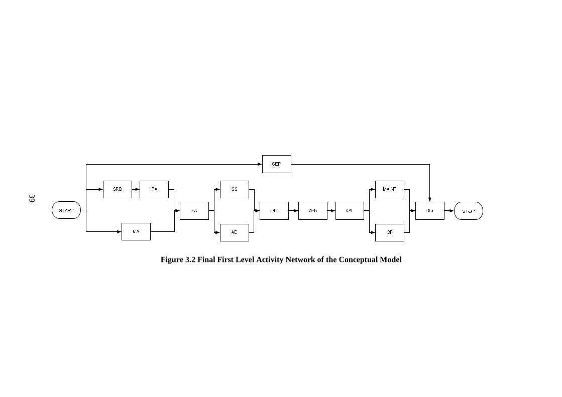
39
Figure 3.2 Final First Level Activity Network of the Conceptual Model

40
Figure 3.3 Partial Second Level Activity Network of the Conceptual Model

41
CHAPTER 4
MODELING OF SYSTEMS ENGINEERING PROCESS IN SYSML
In this chapter, implementation of the Conceptual Model in SysML is described. In
Section 4.1, the SysML model is defined in structural and behavioral aspects and in
Section 4.2, model properties and simulation input parameters are introduced.
4.1 MODELING STRUCTURE AND BEHAVIOR OF THE SYSTEM
Based on the Conceptual Model, which was defined in Chapter 3, Systems
Engineering Process is modeled using the modeling language SysML in the
modeling environment IBM Rational Rhapsody. SysML diagrams provide means to
model the system in terms of its structure, behavior and requirements [9] and
facilitates the reflection of the system to any level of abstraction [3], as introduced
in Chapter 2.
This study focuses on modeling the structure of the system with block definition
diagrams and the behavior of the system with activity diagrams. Since our system of
concern is not a tangible product made of hardware and software, but a process
instead, each system block has its corresponding activity. Therefore, the block
definition diagrams and activity diagrams are interrelated.
4.1.1 Modeling Structure by Block Definition Diagrams
The Conceptual Model includes two levels of activity networks. Thus, a two-level
hierarchy is to be considered while constructing the system structure. The first level
corresponds to Systems Engineering Process structure and the second level
corresponds to the structure of each first level systems engineering activity
.

42
Modeling these two levels enable us to represent the system and subsystems by
structural aspects.
Defining the system as a process, main system units (blocks) indicate process parts
(activities). “Part Association” [9] is used in order to describe the composition
relation among the system block (Systems Engineering Process) and the blocks
representing the subsystems (first level systems engineering activities). Systems
Engineering Process block definition diagram is given in Figure 4.1.
Figure 4.1 Systems Engineering Process Block Definition Diagram
Defining each subsystem as a process, subsystem units also indicate process parts
(subactivities). Again “Part Association” [9] is used in order to describe the
composition relation among a subsystem block and the blocks representing the
components (second level systems engineering activities). Block definition diagram
for sample activity AD is shown in Figure 4.2.
bdd [Package] Architecture [SysEngProcess]
SysEngProcess«b lock»
1
SRD«b lock»
1
RA«b lock»
11 1
MA«block»
1 1
FA«b lock»
1 1
SS«block»
1
AD«b lock»
11
1
INT«b lock»
11
VER«b lock»
1
VAL«b lock»
11 1
MAINT«b lock»
1 1
OP«b lock»
1 1
DIS«b lock»
1 1
SEP«b lock»
1

43
Figure 4.2 Architectural Design Block Definition Diagram
4.1.2 Modeling Behavior by Activity Diagrams
Although behavior of a system can be modeled in several ways in SysML, when a
flow is to be defined as in the case of a process, an activity diagram is a good choice
[3]. Hence, the behavior in Systems Engineering Process is modeled using activity
diagrams. The Conceptual Model included two levels of activity networks, meaning
two levels of flow. Firstly, Systems Engineering Process is modeled considering the
flow of first level systems engineering activities. Then, each systems engineering
activity is modeled considering the flow of second level systems engineering
activities. Therefore, the behavior of the overall system is represented by activity
diagrams.
Highest level behavior is reflected by the activity diagram of overall Systems
Engineering Process. In this activity diagram, each first level systems engineering
activity is indicated by a nested action called “Subactivity” in Rhapsody. Each first
level systems engineering activity includes the relations between related second
level activities.
bdd [Package] Architecture [AD]
AD«block»
AD1«block»
11 1
AD2«block»
1
AD3«block»
11

44
Systems Engineering Process network structure, which includes parallel activities,
is reflected by fork and join nodes. The flow of first level systems engineering
activities within Systems Engineering Process is indicated by an activity diagram as
given in Figure 4.3.
Second level behavior is represented by activity diagrams, each including
subactivities of a first level systems engineering activity. In the activity diagram of
a first level systems engineering activity, second level activities are indicated by
actions. The network structure is again achieved by using fork and join nodes,
where parallel activities are observed. The flow of second level systems engineering
activities of sample activity AD is indicated in Figure 4.4.

45
Figure 4.3 Systems Engineering Process Activity Diagram
act [Package] Architecture [SysEngProcessActivity]
MA
RASRD
FA
SS
AD
SEP
INT VER VAL
MAINT
OP
DIS

46
Figure 4.4 Architectural Design Activity Diagram
AD
AD1
AD2
AD3

47
In addition to the activity diagrams, use case diagrams can also be used for
modeling the behavior [9]. Use case of concern reflects the overall functionality of
conducting systems engineering. The use case diagram for the systems engineering
process is given in Figure 4.5. The actors Systems Engineer (SysEng), Subject
Matter Expert (SME) and Project Manager (PM) represent the roles of the group of
people who are using the system, and also who are being used by the system to
achieve its intended purpose. These actors and their role in simulation will be
explained further in the following section.
Figure 4.5 Systems Engineering Process Use Case Diagram
4.2 MANAGING MODEL PROPERTIES AND INPUT PARAMETERS
After describing the conceptual model implementation in SysML in Section 4.1,
this section includes necessary properties of the final SysML model, before it can
be transformed to ARENA simulation environment.
uc [Package] Architecture [SysEngProcessUseCase]
ConductSystemsEngineering
SysEngSysEng
SMESMEPMPM

48
The proposed SysML model so far represents the structure of the system in terms
of system hierarchy and the behavior in terms of precedence relations. However, a
set of evaluation criteria is needed in order to build different system alternatives
and compare them before setting a baseline to the model. Once the evaluation
criteria (or performance measures) are determined, simulation can be conducted
for system evaluation.
Value of a project, product or process can be improved by achieving a lower total
life cycle cost (using less resource) and meeting schedule objectives, assuming that
the project satisfies all its essential functions and requirements at required levels
[1]. Similarly, timing and cost can be regarded as two of the indicators of project
performance [21]. Assuming that our system-of-concern achieves its functionality
when all activities in the process are completed, project duration and resource
usage can be regarded as indicators of system’s performance or value. In other
words, project duration and resource usages form our evaluation criteria, according
to which different system alternatives can be analyzed.
The abstraction level of the model requires that duration and resource requirements
of second level systems engineering activities are the input parameters to be set for
each system alternative. Duration is the time required for an activity to be
completed in terms of days. Assuming resources other than labor do not differ
among the system alternatives, resource types are defined as follows:
1. Project Manager (PM)
2. Systems Engineer (SysEng)
3. Subject Matter Expert (SME)
Descriptions of the resource types are given below.
Project Manager (PM): Although a PM can be regarded as the person responsible
for planning, implementing and completing the project [21], due to his
concentration on management tasks and limited communication with the
disciplines, the holistic system view might be lost [3]. In this study, a PM is
considered as the person who defines a high level roadmap for the project to
achieve its success criteria, evaluates the effects of the technical risks to the
management and revises the roadmap when required. Since our study assumes that

49
the Project Processes defined in INCOSE [1] flow in parallel to the systems
engineering process, Project Processes are not introduced within the scope of the
study as distinct activities. PM’s participation in the technical part of the systems
engineering process is considered, where more than one PM can be allocated to a
project, representing a project management team.
Systems Engineer (SysEng): SysEng is the connecting link between the disciplines
in the project and is the system level architect [3]. In addition to these, SysEng is
regarded in this study as the technical success enabler, considering the complete
problem [1]. SysEng works close to PM [1], determines technical risks, and
provides possible solutions.
Subject Matter Expert (SME): In this study, SME is considered as any person
participating in the systems engineering activities but not a systems engineer or a
project manager. SME can be a structural engineer, a test engineer, a technician
working at the production line, etc. SME has a knowledge and/or experience in a
particular discipline.
Considering the resource definitions above, the SysML model is updated to
include the resource requirements and duration for every second level systems
engineering activity as well as resource availabilities of the project. In Rhapsody,
resource and duration information are entered in the description tab of related
action as initial values, which can easily be adjusted later on. Resource
availabilities are similarly added in the description tab of related actor.
Although the export interface is provided via XMI in Rhapsody, another method is
followed in this study using the Table View and Table Layout properties. First a
Table Layout is defined to include the actor and activity names in one column and
the actor or activity descriptions (consisting of available resource values, duration
and resource requirements) in the other . Then, a Table view is created to have the
activities and actors in one column and corresponding descriptions in the second
column. In the table, activity descriptions are included only for the second level
systems engineering activities, as expected. An example for a part of the Table
View with initial resource and duration values is given in Figure 4.6 Table View
Example in Rhapsody.

50
Figure 4.6 Table View Example in Rhapsody
With specification of duration and resource requirements for second level
activities, implementation of the conceptual model in SysML is complete. The
implementation includes the minimum set of input parameters necessary for
transforming the model to an Arena simulation model.

51
CHAPTER 5
MODEL TRANSFORMATION FOR SIMULATION
In this chapter, transformation of the SysML model to the Arena simulation model
is described. In Section 5.1, the base Arena model is introduced and in Section 0
transformation process is described.
5.1 BASE ARENA MODEL
In Chapter 4, a SysML model was created reflecting the conceptual model and
including initial values of duration and resource requirements for each second
level systems engineering activity. Within the SysML model, first and second level
activity networks are the main parts and are kept as they are through the simulation
and alternative analysis studies. The conceptual model also provides a basis for the
simulation model, to which the system hierarchy and the flow of first and second
level activities are direct inputs. In order to automate the model transformation, a
base simulation model is created considering the conceptual model together with
initial values of activity durations and resource requirements.
The base model includes Arena representation of the conceptual model. In the
Experiment Frame, following elements are included:
1. Resources: SysEng, SME and PM
2. Queues: Queue1, Queue2, …, Queue25
3. Replicate
4. Tallies: Completion Time

52
In the Model Frame, following blocks and submodels are included:
1. Submodels: A submodel for each first level systems engineering activity
2. Blocks: Create, Duplicate, Queue, Seize, Delay, Release, Match and
Dispose
Therefore, the Model Frame reflects the activity network of the conceptual model
and the Experiment Frame defines resources, queues and replication length in
order to complement the model content for simulation. Arena model view of the
first level activity network is given in Figure 5.1.
Figure 5.1 Arena Model View of the First Level Activity Network
In Figure 5.1, each of the 13 first level activities is represented by an Arena
submodel. A Duplicate block is used after an activity if it has multiple successors.
A Match block is used before an activity when it has multiple predecessors.
MA
RAFAS RD
SS
AD
INT V ER VAL
SEP
MAINT
OP
DIS
Create
Dispose
11
Duplicate
1
Duplicate
1
Duplicate
Match
Match
Match
Queue1
Queue
Queue2
Queue
Queue3
Queue
Queue4
Queue
Queue5
Queue
Queue6
Queue
Queue7
Queue
C ompletionTime
Tally
Queue21Queue22Queue23Queue24Queue25Queue9Queue10Queue11Queue12Queue13Queue14Queue16Queue17Queue18Queue19Queue20Queue15Queue8Queue7Queue5Queue6Queue3Queue4Queue1Queue2
Queues Replicate
S MES ysE ngP M
Resources
C ompletionTime
Tallies
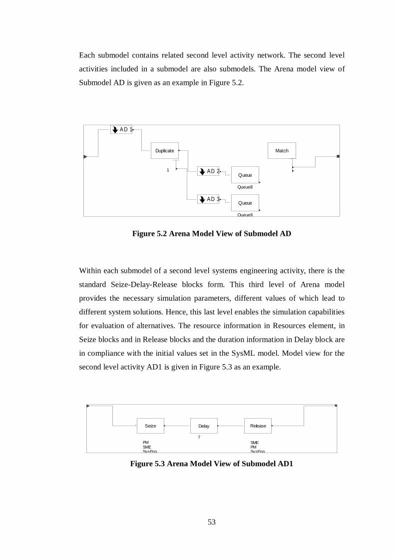
53
Each submodel contains related second level activity network. The second level
activities included in a submodel are also submodels. The Arena model view of
Submodel AD is given as an example in Figure 5.2.
Figure 5.2 Arena Model View of Submodel AD
Within each submodel of a second level systems engineering activity, there is the
standard Seize-Delay-Release blocks form. This third level of Arena model
provides the necessary simulation parameters, different values of which lead to
different system solutions. Hence, this last level enables the simulation capabilities
for evaluation of alternatives. The resource information in Resources element, in
Seize blocks and in Release blocks and the duration information in Delay block are
in compliance with the initial values set in the SysML model. Model view for the
second level activity AD1 is given in Figure 5.3 as an example.
Figure 5.3 Arena Model View of Submodel AD1
A D 1
AD 2
AD 3
1
Duplicate Match
Queue8
Queue
Queue9
Queue
7
Delay
SMEPMSysEng
Release
PMSMESysEng
Seize

54
5.2 MODEL TRANSFORMATION
In Section 5.1, Base Arena Model was defined. This model, together with the
SysML model, establishes the starting point to the model transformation process.
A map of the transformation process is given in Figure 5.4. Once the Modified
Base Model in Excel is obtained, the first two boxes displayed in dashed lines are
omitted for the alternatives analysis. The process is detailed in the following
paragraphs.
Figure 5.4 Model Transformation Process
Base Model in MS Excel
Base Model in Arena
Modified Base Model in MS Excel
SysML Model in Rhapsody
Table View in MS Excel
Simulation Model in MS Excel
Simulation Model in Arena

55
Arena provides interface to both Access and Excel by the export functionality. In
this study, the Excel interface is preferred. The base model is first developed in
Arena and then exported to Excel for further modification. The Base Model in
Excel includes the resource requirements and duration information for the second
level systems engineering activities and resource availability within its tabs,
namely Blocks Seize Resources, Blocks Release Resources, Blocks Delay and
Elements Resources. The rest of the file includes necessary information to build
the model in compliance with the conceptual model. This file is modified to
remove the resource capacities, resource requirements and activity durations to
obtain the Modified Base Model in Excel, which will be used to obtain the final
simulation model with the actual input parameter values.
As described in Chapter 4, Table View of the SysML model includes the activities,
resource requirements and duration values for the activities, and resource
availabilities. This reflects the part of the model that provides the input parameters
and is to be transferred to the simulation environment. Although a SysML model
can be exported as an XMI file, it is not the only method to extract the necessary
information. Since information to be transferred is already included in the Table
View, the table is directly copied to an Excel file. Transformation of the Table
View in Excel to the final Simulation Model in Excel, was achieved via running
VBA codes and using the Modified Base Model in Excel.
The first VBA code named “Rearrange”, firstly copies available resource
quantities to “Elements Resources Resources” tab of the Modified Base Model in
Excel. Then the macro distributes duration and resource requirements to columns
and deletes the rows for first level activities since they do not include any
information to be transferred to the simulation. VBA code for the macro Rearrange
is given in Appendix D.1.
The second and the third VBA codes provide transformation of the file into the
format required by Arena. Using the second VBA code named “Macro_Transfer”,
firstly the activities are listed in the order required by Arena import. Then, activity
duration values are transferred to the “Blocks Delay” tab of the Modified Base
Model in Excel. Afterwards, resource requirements are transferred to “Blocks
Release Resources” tab. Similarly, using the third VBA code named

56
“Macro_Transfer2”, resource requirements are transferred to “Blocks Seize
Resources” tab of the Modified Base Model in Excel. At the end, Simulation
Model in Excel is obtained. VBA codes for Macro_Transfer and Macro_Transfer2
are given in Appendix D.2 and Appendix D.3, respectively. Finally, Simulation
Model in Excel is imported to Arena and “Simulation Model in Arena”, which is
ready to be run, is obtained.
In order to have different system alternatives in the simulation environment, Table
View is updated to reflect the resource requirements and durations of activities in
that alternative. The VBA codes are run on the Table View of concern and the
resultant simulation model in Arena is obtained. Simulation cases for system
alternatives and the run results are discussed in Chapter 6.
57
CHAPTER 6
VERIFICATION CASE STUDIES AND RESULTS
In this chapter, case studies and their results are introduced. In Section 6.1 the
cases, which denote system alternatives, are described. In Section 6.2 simulation
results are given.
It should be noted that the purpose of these cases is only verification as opposed to
validation and true system performance evaluation. Hence, they are hypothetical
cases. Specifically, input parameter values (activity durations, resource
requirements of activities, and resource availabilities) are not estimated based on
data collected from a real life system. They are selected as “reasonable” values
based on past experiences. Therefore, simulation results do not reflect true
performance estimators. They should be used only to verify the model behavior by
comparing the system alternatives based on “reasonable” results.
6.1 CASE STUDIES
Conceptual model formation, model implementation in SysML and model
transformation to Arena for simulation were described in Chapter 3, Chapter 4 and
Chapter 5, respectively. These three chapters describe the modeling and simulation
approach for the systems engineering process of aerospace design projects.
In developing the simulation model, initial input parameter values were used for
several activities as stated in Section 4.2. Although the current Arena model can be
run and simulation results for this unique case can be obtained, the simulation
process is to be extended to verify the simulation model developed in our study. In
order to observe the performance of the system with changing input parameters
and to evaluate system alternatives , different cases are defined in this chapter. The

58
proposed approach is conducted for these cases and simulation results are
obtained. In this section, the cases are introduced.
Cases are determined based on the following three criteria: scale of the project as
“small” or “large”, resource availability as “high” or “low” and activity duration
type as “deterministic” or “stochastic”. Duration of each second level systems
engineering activity and availabilities of each resource type are adjusted
accordingly.
Properties of simulation cases are given in Table 6.1. The first three cases include
deterministic activity durations. D1 can be regarded as the base case, where all
parameters are set to the same values as the initial ones defined for model building
process in Section 4.2. D1 denotes the small scale, low resource availability and
deterministic activity durations. D2 is generated by multiplying the activity
durations of D1 by a factor of 2.0 to obtain the large scale, low resource
availability and deterministic activity durations case. D3 is generated by
multiplying the activity durations and resource availability values of D1 by a
factor of 2.0 to obtain the large scale, large resource availability and deterministic
activity durations case. Individual activity resource requirements and durations for
deterministic cases are given in Table E.1 in Appendix E.
Cases S1, S2 and S3 reflect stochastic activity duration versions of D1, D2 and D3,
respectively. Meredith [21] suggests to use triangular distribution to analyze risk
and manage the uncertainty in activity durations. Also, it is common practice in
simulation to use triangular distribution when there are no data to determine the
probability distributions [22]. Hence, triangular distribution is used in order to set
stochastic activity durations. Minimum and mode values are remained as they are
in the deterministic cases. Maximum values are obtained by multiplying the
minimum/mode values by a factor of 1.5 or 2.0, depending on the risk associated
with each activity. A high risk activity is considered as an activity that might lead
to iterations within the activity itself and hence might have a more extended
duration than expected. For low risk activities value in deterministic case is
multiplied by 1.5. Second level activities of SRD, MA, RA, FA, SS and AD are
treated as high risk activities and the rest as low risk activities. Individual activity

59
resource requirements and durations for stochastic cases are given in Table E.2 in
Appendix E.
Table 6.1 Properties of Simulation Cases
Case Number
Case Description Resource Availability
Activity Durations SysEng SME PM
D1 Small Scale and Low Resource Availability
10 30 2 Constant (c)
D2 Large Scale and Low Resource Availability 10 30 2 Constant (2c)
D3 Large Scale and High Resource Availability
20 60 4 Constant (2c)
S1 Small Scale and Low Resource Availability
10 30 2
Triangular (c, c, 2c) for high risk activities Triangular (c, c, 1.5c) for low risk activities
S2 Large Scale and Low Resource Availability 10 30 2
Triangular (2c, 2c, 4c) for high risk activities Triangular (2c, 2c, 3c) for low risk activities
S3 Large Scale and High Resource Availability
20 60 4
Triangular (2c, 2c, 4c) for high risk activities Triangular (2c, 2c, 3c) for low risk activities

60
6.2 CASE STUDY RESULTS Given the cases to evaluate systems engineering process alternatives in Section
6.1, this section includes simulation results. Before implementing the cases in the
proposed method, a step in model verification is conducted using the critical path
method. Among the initial parameters set in Chapter 4 (also used in Case D1),
activity durations are kept as they are while available resource quantities are
increased to a large figure such as 500, which cannot be reached in all cases, in
order to represent unlimited resources. This parameter set forms the base case.
Following the critical path method for the base case, critical activities are obtained
as follows: SRD1, SRD2, SRD3, RA3, RA4, RA5, FA1, FA2, SS1, SS2, INT1,
INT2, INT3, INT4, INT5, INT6, VER1, VER2, VER3, VER4, VAL1, VAL2,
VAL3, VAL5, VAL6, VAL7, VAL8, MAINT1, MAINT2, MAINT3, MAINT5,
MAINT7 / MAINT8 (Or OP1, OP2, OP3 / OP4 / OP5 instead of MAINT
activities), DIS1, DIS2 / DIS 3, DIS 4, DIS5, DIS6. Project duration for the base
case is obtained as 255, accordingly. Critical path for the first level systems
engineering activities is given in bold in Figure 6.1. Critical path for a section of
second level systems engineering activities is given in Figure 6.2.
In order to complete this step of verification, initial SysML model introduced in
Chapter 4 is modified for unlimited resources, in compliance with the base case.
When the proposed approach is conducted, 255 days are obtained as the project
duration. Hence, the critical path method and the proposed approach resulted in the
same value of project duration for the base case.
Completing this step, the first three cases with deterministic activity durations are
regarded as inputs and the proposed method is run. Firstly, D1 is implemented in
the SysML model, modifying the model to include activity durations, resource
availabilities and resource requirements of D1. Model transformation to Arena and
simulation run are conducted and results are obtained. Results include project
duration in terms of work days and the resource utilizations in percentages. The
same process is repeated for remaining deterministic cases D2 and D3. Results are
included in Table 6.2.

61
Figure 6.1 Critical Path for First Level Activity Network

62
Figure 6.2 Critical Path for Partial Second Level Activity Network

63
Table 6.2 Average Results for Simulation Cases
Base
Case
Case
D1
Case
S1*
Case
D2
Case
S2*
Case
D3
Case
S3*
Critical Path With
Unlimited
Resources
255.0 255.0 310.8 510.0 621.7 510.0 621.7
Project Duration
(Work Days) 255.0 378.0 455.3 756.0 910.7 626.0 758.3
SysEng Utilization
(%) - 34.1 34.8 34.1 34.8 20.6 21.0
SME Utilization
(%) - 51.5 51.7 51.5 51.7 31.1 31.0
PM Utilization (%) - 29.8 29.4 29.8 29.4 18.0 17.9
* For stochastic cases, “critical path” is the sum of the expected durations of
the activities that are on the critical path. Project duration and resource
utilizations are averages of 10 replications.
For the cases with stochastic activity durations (S1, S2 and S3), determining the
number of replications and constructing a confidence interval (CI) is a concern.
As stated in Law and Kelton [22], considering a sample Y1, Y2, …, Ym obtained
from m replications and Y = ∑ Y , if Y1, Y2, …, Ym are independent and
normally distributed, classical estimation theory can be used to construct a CI for
E(Y).
Stochastic activity durations lead to different simulation results in each replication,
in terms of project duration and resource utilizations. Since system state is
initialized at the beginning of each replication, different random variables are used
and the values in each replication are independent from each other [22]. Although
activity durations are subject to triangular distribution, normal distribution can be
assumed according to Central Limit Theorem, since the observed duration in each
replication means completion of all activities and the number of activities is not
small.

64
Having project duration and resource utilizations independent and approximately
normally distributed, a CI is determined in accordance with the algorithm
proposed by Law and Kelton [22]. This algorithm defines the number of
replications by managing the two conflicting objectives: high level of confidence
(small α) and high precision (narrow CI width).
For each of the cases S1, S2 and S3 with stochastic activity durations, the
following steps are conducted to establish/verify the number of replications needed
to obtain the average values of project duration, SysEng utilization, SME
utilization and PM utilization.
1. Initial number of replications is set.
n=n0=10
2. Average value across the replications is calculated.
Y = 1n Y
3. Variance of project duration among the replications is calculated.
s = 1
n − 1 (Y −Y)
4. α is selected as 0.10.
5. CI half length is calculated.
h = t , α/ √
6. Relative precision (r) is selected as 0.10.
7. Desired half length is calculated.
h∗ = rY
8. If h ≤ h∗, iterations are sufficient, algorithm is terminated with CI Y ± h.
Otherwise, the number of iterations is updated.
n∗ = nhh∗ + 1
n is set to n*.
Steps 1 to 8 are repeated.
The above algorithm is used for project duration in case S1 as an example below.

65
1. n=n0=10
2. Y = ∑ Y = (460.3 + 476.4 + 448.7 + 445.1 + 452.5 +
447.6 + 457.0 + 448.0 + 452.2 + 465.5)
Y = 455.3
3. Variance of project duration among the replications is calculated.
s = ∑ (Y −Y) = ((460.3− 455.3) + (476.4− 455.3) +
(448.7− 455.3) + (445.1− 455.3) + (452.5− 455.3) +
(447.6− 455.3) + (457.0− 455.3) + (448.0− 455.3) +
(452.2− 455.3) + (465.5− 455.3) )
s = 94.8
4. α is selected as 0.10.
5. CI half length is calculated using t-distribution [22].
h = t , . √= 1.83 .
√
h = 5.6
6. Relative precision (r) is selected as 0.10.
7. Desired half length is calculated.
h∗ = rY = (0.10)(455.3)
h∗ = 45.5
8. Since h ≤ h∗, algorithm is terminated with CI 455.3± 5.6.
Therefore, 10 replications are sufficient for project duration estimation in S1. The
same outcome is observed for the other simulation cases. For each of the cases S1,
S2 and S3 with stochastic activity durations; 10 replications are found sufficient
for a reasonable estimation of project duration, SysEng utilization, SME utilization
and PM utilization. Step-by-step results for replication number estimation
algorithm are given in Appendix F. Confidence intervals for stochastic simulation
cases are summarized Table 6.3.

66
Table 6.3 Confidence Intervals for Stochastic Simulation Cases (훂=0.10)
Case S1 Case S2 Case S3
Standard
Deviation
Confidence
Interval Limits
Standard
Deviation
Confidence
Interval Limits
Standard
Deviation
Confidence
Interval Limits
Project Duration* 3.1 449.7, 461.0 6.2 899.4, 922.0 7.1 745.3, 771.3
SysEng Utilization (%)* 0.2 34.5, 35.2 0.2 34.5, 35.2 0.1 20.7, 21.2
SME Utilization (%)* 0.2 51.3, 52.1 0.2 51.3, 52.1 0.3 30.5, 31.6
PM Utilization (%)* 0.3 28.9, 29.9 0.3 28.9, 29.9 0.2 17.5, 18.4
* Project duration and utilization results are based on 10 replications
.

67
CHAPTER 7
CONCLUSIONS
The primary aim of this study is to model the systems engineering process of an
aerospace design project and to generate a simulation model in order to evaluate
the system performance. Although there exists a general understanding of the
systems engineering concept, there is no unique definition for the process of
systems engineering in terms of the activities included. The activities included, as
well as the flow of these activities, depend highly upon the project of concern (i.e.
modernization project, design project, production-only project etc.). This study
considers systems engineering process of a real-life design project, addressing the
whole life-cycle of the product. Product domain is identified as aerospace but no
further limitations are specified.
A two-phase survey study is conducted in order to obtain a conceptual model for
the systems engineering process. In each phase, ten systems engineers working in
Helicopter Group in Turkish Aerospace Industries Inc. participated and stated their
opinions related with the systems engineering process of a design project. The
survey study is based on two references: Technical Processes defined in INCOSE
Systems Engineering Handbook [1] and Systems Engineering Processes given in
“Fundamentals of Modern Systems Engineering” short course of Georgia Tech [5].
At the end of the first phase, first level systems engineering activity network is
obtained. This first level network provides an input to the second phase, where
second level activity networks are defined. Hence, the conceptual model includes
two levels of activity networks. One reason for this is the content of the references
and another is to have a practical and reasonable model, which can further be
developed to meet the needs of simulation. However, the model building

68
methodology introduced in this study, has capabilities to reflect any level of
abstraction due to object-oriented modeling characteristics.
Another aim is to implement the conceptual model in the object-oriented modeling
environment, which provides a proper interface to systems engineers, project
managers and even to the customer. SysML is used as the modeling language,
since it is a standard language in systems engineering domain. Among the several
diagram types that SysML features, block definition diagrams and activity
diagrams are used in our study. By using block definition diagrams, the structural
view of the system is defined, providing the hierarchical relations between system
elements. On the other hand, activity diagrams reflect the behavior of the system
by including the flow of activities.
In this study we also aim to transform the SysML model to a simulation
environment and run the simulation to obtain results related with certain system
characteristics such as project duration and resource utilizations. Therefore, an
initial set of required parameters are embedded in the SysML model. These are
resource availabilities, activity durations, and resource requirements of activities.
The conceptual model is implemented in Arena to obtain a base model. The
necessary parameters of the SysML model are then transferred to Excel and the
final Excel file is obtained through VBA codes. By importing this final file to
Arena, model to be simulated is achieved.
An ideal model is the one which can be verified and validated. By modifying the
initial set of parameters in SysML model for unlimited resource availabilities and
by applying the proposed method accordingly, project duration with unlimited
resource availabilities is obtained. This result is compared by the manual critical
path calculation and it is observed that the two results are compliant. Then, case
studies are conducted to evaluate the system alternatives, which differ in scale of
the project, in resource availabilities and also in the type of activity durations as
deterministic or stochastic. Hence there are three cases for each of the
deterministic and stochastic activity duration versions: small scale and low
resource availability case, large scale and low resource availability case, large
scale and high resource availability case.

69
The scale of the project is set as large or small by adjusting the activity durations.
Similarly resource availabilities are changed among cases to evaluate its effect on
the overall process. For stochastic activity durations, the deterministic values are
taken as the minimum and mode of the triangular distribution and the maximum
value is set as a factor of minimum/mode, where the factor depends on the risk
expected for an activity.
As a result of the case studies, it is observed that project duration for stochastic
activity duration cases are always higher than those of deterministic activity
duration cases, as expected. When unlimited resources are assumed, small scale
cases have shorter project durations than high scale cases. Assigning limited
resource availabilities, the project duration increases in the order of small scale and
low resource availability cases, large scale and large resource availability cases,
large scale and low resource availability cases.
SME has the highest utilization values in all cases, followed by SysEng. PM has
the lowest utilization. This is also expected since SMEs have different expertise
areas and participate in several different steps of the whole process, while PMs
take part in technical processes only when required.
Increasing the scale of the project does not affect the utilization value of any of the
resources but leads to higher project completion times. This is expected since
available resource quantities stay the same. Comparing two large scale cases, it is
observed that with increasing resource availability, project completion time
decreases both in deterministic and stochastic cases, while the utilization values
drop. Hence, allocating resources to more than one project might be suitable for
systems engineering process.
Prior to model building, the problem domain was set as a design project of
aerospace products. Considering the design of less complex vehicles, might reduce
the complexity of the conceptual model and might lead to a simpler model
implementation, transformation and simulation process. On the other hand, design
of a more complex system might require a higher abstraction level.
The conceptual model is based on two references. Although they’re well-known
and authoritative in the field of systems engineering, the number of references can

70
be extended in further studies or a new activity set can be formed by a larger group
of people having knowledge and experience on the subject. The survey study
respondents in this study are systems engineers, who have been working on real-
life projects. However, they are experienced mainly in the aerospace domain.
Therefore, shifting the domain would require to extend or to change the respondent
profile. Two levels of networks are included within the conceptual model.
Although this fits the projects of concern in our study, it should be noted that, with
introduction of the second level networks, setting predecessor relations becomes
more challenging for the survey respondents. Also the process of evaluating
survey results becomes more complicated, which might lead to a decrease in the
similarity of the conceptual model to a real life project.
While forming the second level activity networks in Phase 2 of the survey, second
level activities of only the selected first level activities are used. Hence, only one
of the two references is considered for each second level activity network. Another
approach would be to combine the second level activities of the two references and
ask the respondents to select the required ones from this mixed set. This is a more
flexible solution but also more complicated since each of the references has their
own detailed definitions of the second level activity groups. Moreover, in this case
an additional step of selecting the second level activities before forming the
networks would be added to Phase 2 of the survey.
Phase 2 of the survey is in compliance with the results of Phase 1. However, no
iterations are followed. Although one of the group decision making techniques (i.e.
Delphi technique, brainstorming etc.) were intended to be used, since the
respondents had limited amount of time and since the available hours differed
from person to person, surveys were conducted individually and once for each
phase. Having no feedback from the final conceptual model to the respondents, the
conceptual model could not be validated. A future study might consider a group
decision making technique, which leads to conceptual model validation.
Model implementation in SysML, includes using activity diagrams and block
definition diagrams. However, SysML offers a wide range of diagrams, each
representing the system from a different perspective. Future studies might include

71
modeling the inputs and outputs among system blocks, as well as modeling the
requirements and their relations with the system.
Transformation of the SysML model to the simulation environment requires a base
model to be created in Arena. The process of model transformation can be
improved to omit the need for base model creation, being able to automatically
create the necessary features in Excel. Using VBA codes to transform the SysML
output to the necessary file for importing the model to Arena is an alternative
approach to using XMI export functionality of SysML. However, the first step
requires a manual copy-paste step, to transfer the SysML table view to the Excel
file. In a future study, this process can be made fully-automatic by combining the
use of XMI and VBA codes.
The cases formed for alternatives are hypothetical examples and are not based on
data obtained from real life projects. Hence, the cases do not generate true
estimates. They only provide examples to illustrate possible applications and
verification of the proposed approach. Therefore, future work might include a
specific case study, reflecting collection and statistical analysis of real life data.
In the case studies, the scale of the project is assumed to be dependent on the
activity durations but not on the resource requirements of activities. Hence,
activity durations are increased to simulate large scale. However, larger project
scales can also be simulated considering higher resource requirements for
activities. Moreover, a factor of two is used to multiply the small scale durations to
obtain large scale durations for all activities. More realistic data can lead to
different factors for different activities, since certain activity durations might only
be slightly affected by the scale of the project (i.e. mission analysis) while others
depend highly on the scale (i.e. integration). Regarding resource availabilities,
again a factor of two is used to multiply the low resource availability cases to
obtain high resource availability cases. Similarly, this factor can be re-adjusted
according to more realistic data since high resource availability might mean higher
quantities for certain resource types (i.e. SME) than the others (i.e. PM).
In order to observe the effect of uncertainty on the project performance, stochastic
durations are assigned to activities. Triangular distribution is assumed since

72
statistical data are not available and since stochastic durations is preferred to be
easily related to the respective deterministic values. However, valid statistical data
might fit better to another distribution. The effect of high risk is reflected on the
project duration while maximum values of the triangular distribution is assigned.
Activities up to integration are assumed to be high risk, due to the iterative nature
of these activities at the initial stages of the project life cycle. However, the effect
of risk originating from a high risk activity might also be observed at another stage
(i.e. at later stages) of the project life cycle and hence might affect the duration of
other activities as well. Defining high risk activities according to real-life
statistical data and analyzing the effects of risk are considered as other future
perspectives.
The proposed approach is considered as applicable to project management
problems, providing certain advantages over the well-known project management
tools and methods. Firstly, a realistic process network is achieved for design
projects, where respondents are from the domain of concern and where their
experiences are taken into consideration. Secondly, the approach allows
conducting sensitivity analysis by assigning different resource availabilities and
different resource requirements and durations for the activities. Hence the
proposed approach does not address a pure scheduling solution but also provides
means for “what if” analysis facilitating workload and activity duration estimation.
Finally, the object-oriented methodology provides future extension capabilities to
include the physical model of the product and link it to the processes obtained in
this study.
In general, different phases of this thesis study such as systems engineering
process definition, object-oriented model implementation, model transformation
for simulation and sensitivity analysis are applicable for today’s complex system
design and project management issues and are subject to further studies and
improvements.

73
REFERENCES
[1] International Council on Systems Engineering (INCOSE), “Systems
Engineering Handbook”, Version 3.2, 2010
[2] Joint OSD/Services/Industry Working Group, “MIL-STD-499B (DRAFT),
Draft Military Standard: Systems Engineering”, 1993
[3] Weilkiens, T., “Systems Engineering with SysML/UML”, Morgan
Kaufmann OMG Press, 2008
[4] Arnold, S., Lawson, H.W., “Viewing Systems from a Business
Management Perspective: The ISO/IEC 15288 Standard”, Systems
Engineering, vol. 7, iss. 3, pp. 229–242, Wiley Subscription Services, Inc.,
2004
[5] Georgia Institute of Technology, Short Course: “Fundamentals of Modern
Systems Engineering”, Georgia Tech Distance Learning and Professional
Education, 2011
[6] Booch, G., “Object-oriented Analysis and Design”, 2nd ed., Addison-
Wesley Longman, 1994
[7] Object Management Group (OMG), “OMG Unified Modeling LanguageTM
(OMG UML), Infrastructure Specification”, Version 2.4.1, 2011
[8] Object Management Group (OMG), “OMG Unified Modeling LanguageTM
(OMG UML), Superstructure Specification”, Version 2.4.1, 2011
[9] Object Management Group (OMG), “OMG Systems Modeling Language
(OMG SysMLTM) Specification”, Version 1.3, 2012

74
[10] Anglani, A., Grieco, A., Pacella, M., Tolio, T., “Object-oriented Modeling
and Simulation of Flexible Manufacturing Systems: a Rule-based
Procedure”, Simulation Modelling Practice and Theory, vol. 10, no. 3-4,
pp. 209-234, 2002
[11] Constant, O., Monin, W., Graf, S., “A Model Transformation Tool for
Performance Simulation of Complex UML Models”, Companion of the
30th International conference on Software engineering, pp. 923-924, 2008
[12] Huang, E., Ramamurthy, R., McGinnis, L.F., “System and Simulation
Modeling Using SysML”, Proceedings of the 2007 Winter Simulation
Conference, 2007
[13] Liehr, A.W., Buchenrieder, K.J., “An XML Based Simulation Method for
Extended Queuing Networks”, Proceedings of the 22nd European
Conference on Modelling and Simulation, pp. 322–328, 2008
[14] Liehr, A.W., Buchenrieder, K.J., “Transforming UML-Based System
Descriptions into Simulation Models as Part of System Development
Frameworks”, 12th International Conference on Computer Aided Systems
Theory Lecture Notes in Computer Science, vol. 5717, pp.857-864, 2009
[15] Johnson, T., Paredis, C.J.J., Burkhart, R., “Integrating Models and
Simulations of Continuous Dynamics into SysML”, Proceedings of
Modelica Conference, 2008
[16] Nikolaidou, M., Dalakas, Mitsi, L., Kapos, G., Anagnostopoulos, D., “A
SysML Profile for Classical DEVS Simulators”, Proceedings of
International Conference on Software Engineering Advances, pp. 445–450,
2008
[17] Wang, R., Dagli, C.H., “An Executable System Architecture Approach to
Discrete Events System Modeling Using SysML in Conjunction with
Colored Petri Net”, Proceedings of IEEE Systems Conference, pp. 1–8,
2008

75
[18] Nikolaidou, M., Dalakas, V., Anagnostopoulos, D., "Integrating Simulation
Capabilities in SysML using DEVS", Proceedings of IEEE Systems
Conference, 2010
[19] Schönherr, O., Rose, O., “First Steps Towards A General Sysml Model For
Discrete Processes In Production Systems”, Proceedings of the 2009
Winter Simulation Conference, 2009
[20] McGinnis, L., Ustun, V., “A Simple Example Of Sysml-Driven
Simulation”, Proceedings of the 2009 Winter Simulation Conference, 2009
[21] Meredith, J.R., Mantel, S.J., “Project Management: A Managerial
Approach”, 6th ed., John Wiley & Sons, 2006
[22] Law, A.M., Kelton, W.D., “Simulation Modeling & Analysis”, 2nd ed.,
McGraw-Hill, 1991

76
APPENDIX A
QUESTIONNAIRE SURVEY STUDIES
A.1 QUESTIONNAIRE SURVEY STUDY – PHASE 1
QUESTIONNAIRE 1 – Systems Engineering Process First Level Activities
Name:
Surname:
Number of years of work experience in systems engineering:
PART 1
In the following table, a list of potential activities and their purposes/definitions are given
according to two widely accepted systems engineering references. Please read the
purpose/definition of each activity and check the “Included or Not” column, if you think
the corresponding activity should be included and identified separately in the systems
engineering process of a real-world design project conducted in your organization.
If you think that two or more activities overlap, please choose the one you prefer the most
according to the process definitions.
If you think that the activity is a subactivity of another main activity, please leave the box
unchecked. This questionnaire should include only the first level (high level) activities
.

77
Activity
Code
Reference 1
Activity Name
and Purpose
Reference 2
Activity Name
and Purpose
Included or
Not
SRD Stakeholder Requirements
Definition
Define the requirements for a
system that can provide the
services needed by users and
other stakeholders in a defined
environment
MA Mission Analysis
Determine problem /
opportunity, identify potential
customers and stakeholder,
collect high-level desirements
RA Requirements Analysis
Transform the stakeholder,
requirement-driven view of
desired services into a
technical view of a required
product that could deliver
those services
Requirements Analysis
Define system customers,
determine requirements from
desirements, validate system
requirementswith system
customers
BM Baseline Management:
Establish initial system
baselines, control changes to
baselines as system definition
matures
FA Functional Analysis
Identify system functionality in
generic terms, validate
completeness of functional
system description
TS Tradeoff Studies
Study various means of
providing system functionality,
remove unacceptable candidates
from further consideration,
identify any risks associated
with acceptable functional
candidates
AA Alternative Analysis
Combine acceptable functions
into alternative total system
solutions, assess performance of
system alternatives, select one
or more preferred solutions
SS System Synthesis
Identify physical components of
preferred system solution(s),
develop physical system
architectures

78
Activity
Code
Reference 1
Activity Name
and Purpose
Reference 2
Activity Name
and Purpose
Included or
Not
AD Architectural Design
Synthesize a solution that
satisfies system requirements
IMP Implementation
Realize a specified system
element
INT Integration
Assemble a system that is
consistent with the
architectural design
Systems Integration
Define interfaces between
physical system components,
define interfaces between system
and environment, determine
controls and characteristics of
all interfaces
VER Verification
Confirm that the specified
design requirements are
fulfilled by the system
System Verification
Test, inspect, simulate, etc. the
physical architecture of
preferred system solutions,
identify and resolve any non-
compliance with requirements
TRANS Transition
Establish a capability to
provide services specified by
stakeholder requirements in the
operational environment
VAL Validation
Provide objective evidence that
the services provided by a
system when in use comply
with stakeholders’
requirements, achieving its
intended use in its intended
environment
OP Operation
Use the system in order to
deliver its services
MAINT Maintenance
Sustain the capability of the
system to provide a service
DIS Disposal
End the existence of a system
entity
SEP Systems Engineering Planning
Plan for the total systems
engineering effort on a project,
integrate with project
management activities

79
PART 2
Please construct a precedence network including the activities you selected in Part 1 and
using the activity codes in the table.
Your network should look like this:
Precedence Network
Activity 4 Activity 1 Activity 5 Activity 4
Activity 2
Activity 3

80
A.2 QUESTIONNAIRE SURVEY STUDY – PHASE 2
QUESTIONNAIRE 2 – Systems Engineering Process Second Level Activities
Name:
Surname:
Number of years of work experience in systems engineering:
PART 1
In the following table, three activities and corresponding subactivities are given according
to two widely accepted systems engineering references. Please read the activities &
subactivities and in the last column note the name of reference (as “Reference 1” or
“Reference 2”) which you think includes the most appropriate subactivities for the related
activity.
Activity Reference 1
Subactivities
Reference 2
Subactivities
Selected
Reference
RA
Requirements
Analysis
1. Define the System
Requirements
2. Analyze and
Maintain the System
Requirements
1. Define System
Customers
2. Determine
Requirements from
“desirements”
3. Validate system
requirements with
system customers
INT
Integration
Plan Integration
1. Define integration
strategy
2. Schedule integration
testing tools and
facilities
Perform Integration
3. Assemble system
elements according
to the integration
plan
4. Validate and Verify
Interfaces
5. Verify and Analyze
Assemblies
6. Document
integration testing
and analysis results
7. Document and
control the
architectural baseline
1. Define interfaces
between physical
system
components
2. Define interfaces
between system
and environment
3. Determine control
and characteristics
of all interfaces

81
Activity Reference 1
Subactivities
Reference 2
Subactivities
Selected
Reference
VER
Verification
Plan Verification
1. Schedule, confirm
and install
verification enabling
systems
Perform Verification
2. Develop verification
procedures
3. Conduct verification
activities per
established
procedures, to
demonstrate
compliance with
requirements
4. Document
verification results
and enter data into
the Requirements
Verification and
Traceability Matrix
1. Test, inspect,
simulate, etc. the
physical
architecture of
preferred system
solutions
2. Identify and
resolve any non-
compliance with
requirements

82
PART 2
An activity and corresponding subactivities are given in each of the tables below. For each
activity, please read the subactivities and construct a precedence network including the
subactivities. While constructing the network please use the subactivity codes, which are
given in parenthesis following each subactivity name.
For Requirements Analysis (RA), Integration (INT) and Verification (VER) activities,
please use all of the subactivities corresponding to your reference selection in Part 1.
For rest of the activities, please use all of the subactivities given in related table.
A network should look like this:
1. Stakeholder Requirements Definition:
Activity Subactivities and Subactivity Codes
SRD
Stakeholder Requirements
Definition
1. Elicit stakeholder requirements (SRD1)
2. Define stakeholder requirements (SRD2)
3. Analyze and maintain stakeholder requirements
(SRD3)
Precedence Network for Stakeholder Requirements Definition:
Activity 4 Activity 1 Activity 5 Activity 4
Activity 2
Activity 3

83
2. Mission Analysis:
Activity Subactivities and Subactivity Codes
MA
Mission Analysis
1. Determine problem/opportunity (MA1)
2. Identify potential customers and stakeholder
(MA2)
3. Collect high-level desirements (MA3)
Precedence Network for Mission Analysis:
3. Requirements Analysis:
Activity Reference 1
Subactivities and Subactivity
Codes
Reference 2
Subactivities and Subactivity
Codes
RA
Requirements
Analysis
1. Define the system
requirements (RA1)
2. Analyze and maintain the
system requirements
(RA2)
1. Define System Customers
(RA3)
2. Determine Requirements from
“desirements” (RA4)
3. Validate system requirements
with system customers (RA5)
Precedence Network for Requirements Analysis:
4. Functional Analysis:
Activity Subactivities and Subactivity Codes
FA
Functional Analysis
1. Identify system functionality in generic terms
(FA1)
2. Validate completeness of functional system
description (FA2)
Precedence Network for Functional Analysis:
5. System Synthesis:
Activity Subactivities and Subactivity Codes
SS
System Synthesis
1. Identify physical components of preferred
system solution(s) (SS1)
2. Develop physical system architectures (SS2)
Precedence Network for System Synthesis:

84
6. Architectural Design:
Activity Subactivities and Subactivity Codes
AD
Architectural Design
1. Define the architecture (AD1)
2. Analyze and evaluate the architecture (AD2)
3. Document and maintain the architecture (AD3)
Precedence Network for Architectural Design:
7. Integration:
Activity Reference 1
Subactivities and Subactivity
Codes
Reference 2
Subactivities and Subactivity
Codes
INT
Integration
Plan Integration
1. Define the integration
strategy (INT1)
2. Schedule integration
testing tools and facilities
(INT2)
Perform Integration
3. Assemble system elements
according to the
integration plan (INT3)
4. Validate and verify
interfaces (INT4)
5. Verify and analyze
assemblies (INT5)
6. Document integration
testing and analysis results
(INT6)
7. Document and control the
architectural baseline
(INT7)
1. Define interfaces between
physical system components
(INT8)
2. Define interfaces between
system and environment
(INT9)
3. Determine control and
characteristics of all interfaces
(INT10)
Precedence Network for Integration:

85
8. Verification:
Activity Reference 1
Subactivities and Subactivity
Codes
Reference 2
Subactivities and Subactivity
Codes
VER
Verification
Plan Verification
1. Schedule, confirm and
install verification
enabling systems (VER1)
Perform Verification
2. Develop verification
procedures (VER2)
3. Conduct verification
activities, per established
procedures, to
demonstrate compliance
with requirements (VER3)
4. Document verification
results and enter data into
the Requirements
Verification and
Traceability Matrix
(VER4)
1. Test, inspect, simulate, etc. the
physical architecture of
preferred system solutions
(VER5)
2. Identify and resolve any non-
compliance with requirements
(VER6)
Precedence Network for Verification:

86
9. Validation:
Activity Subactivities and Subactivity Codes
VAL
Validation
Plan Validation
1. Develop a validation strategy (VAL1)
Perform Validation
2. Develop validation procedures that demonstrate
that the system is fit for its purpose and satisfies
the stakeholders’ requirements (VAL2)
3. Ensure readiness to conduct validation (VAL3)
4. Support in-process validation throughout
system development (VAL4)
5. Conduct validation to demonstrate conformance
to stakeholder requirements (VAL5)
6. If anomalies are detected, analyze for corrective
actions and detect trends in failure to find
threats to the system and evidence of design
errors (VAL6)
7. Recommend corrective actions and obtain
stakeholder acceptance of validation results
(VAL7)
8. Document validation results and enter data into
the Requirements Verification and Traceability
Matrix (VAL8)
Precedence Network for Validation:

87
10. Maintenance:
Activity Subactivities and Subactivity Codes
MAINT
Maintenance
Plan Maintenance
1. Establish a maintenance strategy (MAINT1)
2. Define maintenance constraints on the system
requirements (MAINT2)
3. Obtain the enabling systems, system elements
and other services used for maintenance of the
system (MAINT3)
4. Monitor replenishment levels of spare parts
(MAINT4)
5. Manage the skills and availability of trained
maintenance personnel (MAINT5)
Perform Maintenance
6. Implement maintenance and problem resolving
procedures (MAINT6)
7. Maintain a history of failures, actions taken and
other trends to inform operations and
maintenance personnel and other projects
creating or utilizing similar system elements
(MAINT7)
8. Monitor customer satisfaction with system and
maintenance support (MAINT8)
Precedence Network for Maintenance:
11. Operation:
Activity Subactivities and Subactivity Codes
OP
Operation
1. Prepare for operation (OP1)
2. Perform operational activation and check-out
(OP2)
3. Use system for operations (OP3)
4. Perform operational problem resolution (OP4)
5. Support the customer (OP5)
Precedence Network for Operation:

88
12. Disposal:
Activity Subactivities and Subactivity Codes
DIS
Disposal
Plan Disposal
1. Review the concept of disposal (DIS1)
2. Define the disposal strategy (DIS2)
3. Impose associated constraints on the system
requirements (DIS3)
Perform Disposal
4. Deactivate the elements to be terminated (DIS4)
5. Disassemble the elements for ease of handling
(DIS5)
6. Remove the elements and any associated waste
products from the operational site (DIS6)
Finalize the Disposal
7. Maintain the documentation of all disposal
activities and residual hazards (DIS7)
Precedence Network for Disposal:
13. Systems Engineering Planning:
Activity Subactivities and Subactivity Codes
SEP
Systems Engineering Planning
1. Plan for the total systems engineering effort on
a project (SEP1)
2. Integrate with project management activities
(SEP2)
Precedence Network for Systems Engineering Planning:

89
APPENDIX B
SURVEY STUDY RESULTS
Table B.1 Predecessor Selection in Phase 1
Respondent Reference (j):
Activity (i)
Candidate
Predecessors for
Activity i (k):
1 2 3 4 5 6 7 8 9 10
SRD
MA 0 0 0 0 0 0 0 1 0 0
RA 0 0 0 0 0 0 0 0 0 0
FA 0 0 0 0 0 0 0 0 0 0
SS 0 0 0 0 0 0 0 0 0 0
AD 0 0 0 0 0 0 0 0 0 0
INT 0 0 0 0 0 0 0 0 0 0
VER 0 0 0 0 0 0 0 0 0 0
VAL 0 0 0 0 0 0 0 0 0 0
OP 0 0 0 0 0 0 0 0 0 0
MAINT 0 0 0 0 0 0 0 0 0 0
DIS 0 0 0 0 0 0 0 0 0 0
SEP 0 0 0 0 0 0 0 1 0 0
MA
SRD 0 0 1 0 0 1 0 0 0 0
RA 0 0 0 0 0 0 0 0 0 0
FA 0 0 0 0 0 0 0 0 0 0
SS 0 0 0 0 0 0 0 0 0 0
AD 0 0 0 0 0 0 0 0 0 0
INT 0 0 0 0 0 0 0 0 0 0
VER 0 0 0 0 0 0 0 0 0 0
VAL 0 0 0 0 0 0 0 0 0 0
OP 0 0 0 0 0 0 0 0 0 0
MAINT 0 0 0 0 0 0 0 0 0 0
DIS 0 0 0 0 0 0 0 0 0 0
SEP 1 0 0 0 0 0 0 1 1 0

90
Table B.1 Predecessor Selection in Phase 1 (Continued)
Respondent Reference (j):
Activity (i)
Candidate
Predecessors for
Activity i (k):
1 2 3 4 5 6 7 8 9 10
RA
SRD 0 0 1 0 0 1 1 0 0 1
MA 1 1 0 0 1 0 0 1 1 0
FA 0 0 0 0 0 0 0 0 0 0
SS 0 0 0 0 0 0 0 0 0 0
AD 0 0 0 0 0 0 0 0 0 0
INT 0 0 0 0 0 0 0 0 0 0
VER 0 0 0 0 0 0 0 0 0 0
VAL 0 0 0 0 0 0 0 0 0 0
OP 0 0 0 0 0 0 0 0 0 0
MAINT 0 0 0 0 0 0 0 0 0 0
DIS 0 0 0 0 0 0 0 0 0 0
SEP 1 0 0 0 0 0 0 1 1 0
FA
SRD 0 0 1 0 0 1 1 1 0 0
MA 1 1 1 0 1 1 0 1 1 0
RA 1 1 1 1 1 1 1 1 1 0
SS 0 0 0 0 0 0 0 0 0 0
AD 0 0 0 0 0 0 0 0 0 0
INT 0 0 0 0 0 0 0 0 0 0
VER 0 0 0 0 0 0 0 0 0 0
VAL 0 0 0 0 0 0 0 0 0 0
OP 0 0 0 0 0 0 0 0 0 0
MAINT 0 0 0 0 0 0 0 0 0 0
DIS 0 0 0 0 0 0 0 0 0 0
SEP 1 0 0 0 0 0 0 1 1 0
SS
SRD 0 0 1 0 0 1 0 1 0 0
MA 0 1 1 0 1 1 0 1 1 0
RA 0 1 1 0 1 1 0 1 1 0
FA 0 1 1 0 1 1 0 1 1 0
AD 0 0 0 0 0 0 0 0 0 0
INT 0 0 0 0 0 0 0 0 0 0
VER 0 0 0 0 0 0 0 0 0 0
VAL 0 0 0 0 0 0 0 0 0 0
OP 0 0 0 0 0 0 0 0 0 0
MAINT 0 0 0 0 0 0 0 0 0 0
DIS 0 0 0 0 0 0 0 0 0 0
SEP 0 0 0 0 0 0 0 1 1 0
AD
SRD 0 0 0 0 0 0 1 1 0 1
MA 1 1 0 0 0 0 0 1 1 0
RA 1 1 0 1 0 0 1 1 1 1
FA 1 1 0 1 0 0 1 1 0 0
SS 0 1 0 0 0 0 0 0 0 0
INT 0 0 0 0 0 0 0 0 0 0
VER 0 0 0 0 0 0 0 0 0 0
VAL 0 0 0 0 0 0 0 0 0 0
OP 0 0 0 0 0 0 0 0 0 0
MAINT 0 0 0 0 0 0 0 0 0 0
DIS 0 0 0 0 0 0 0 0 0 0
SEP 1 0 0 0 0 0 0 1 1 0
INT
SRD 0 0 1 0 0 1 1 1 0 1
MA 1 1 1 0 1 1 0 1 1 0
RA 1 1 1 1 1 1 1 1 1 1

91
Table B.1 Predecessor Selection in Phase 1 (Continued)
Respondent Reference (j):
Activity (i)
Candidate
Predecessors for
Activity i (k):
1 2 3 4 5 6 7 8 9 10
FA 1 1 1 1 1 1 1 1 1 0
SS 0 1 1 0 1 1 0 1 1 0
AD 1 1 0 1 0 0 1 1 1 1
VER 0 0 0 0 0 0 0 0 0 0
VAL 0 0 0 0 0 0 0 0 0 0
OP 0 0 0 0 0 0 0 0 0 0
MAINT 0 0 0 0 0 0 0 0 0 0
DIS 0 0 0 0 0 0 0 0 0 0
SEP 1 0 0 0 0 0 0 1 1 0
VER
SRD 0 0 1 0 0 1 1 1 0 1
MA 1 1 1 0 1 1 0 1 1 0
RA 1 1 1 1 1 1 1 1 1 1
FA 1 1 1 1 1 1 1 1 1 0
SS 0 1 1 0 1 1 0 1 1 0
AD 1 1 0 1 0 0 1 1 1 1
INT 1 1 1 1 1 1 1 1 1 1
VAL 0 0 0 0 0 0 0 0 0 0
OP 0 0 0 0 0 0 0 0 0 0
MAINT 0 0 0 0 0 0 0 0 0 0
DIS 0 0 0 0 0 0 0 0 0 0
SEP 1 0 0 1 0 0 0 1 1 0
VAL
SRD 0 0 1 0 0 1 1 0 0 1
MA 1 1 1 0 1 1 0 0 1 0
RA 1 1 1 1 1 1 1 0 1 1
FA 1 1 1 1 1 1 1 0 1 0
SS 0 1 1 0 1 1 0 0 1 0
AD 1 1 0 1 0 0 1 0 1 1
INT 1 1 1 1 1 1 1 0 1 1
VER 0 1 1 0 0 1 0 0 1 1
OP 0 0 0 0 0 0 0 0 0 0
MAINT 0 0 0 0 0 0 0 0 0 0
DIS 0 0 0 0 0 0 0 0 0 0
SEP 1 0 0 1 0 0 1 0 1 0
OP
SRD 0 0 1 0 0 1 1 0 0 1
MA 0 1 1 0 0 1 0 0 0 0
RA 0 1 1 0 0 1 1 0 0 1
FA 0 1 1 0 0 1 1 0 0 0
SS 0 1 1 0 0 1 0 0 0 0
AD 0 1 0 0 0 0 1 0 0 1
INT 0 1 1 0 0 1 1 0 0 1
VER 0 1 1 0 0 1 0 0 0 1
VAL 0 1 1 0 0 1 1 0 0 0
MAINT 0 0 0 0 0 0 0 0 0 0
DIS 0 0 0 0 0 0 0 0 0 0
SEP 0 0 0 0 0 0 1 0 0 0
MAINT
SRD 0 0 1 0 0 1 1 0 0 1
MA 1 0 1 0 0 1 0 0 0 0
RA 1 0 1 1 0 1 1 0 0 1
FA 1 0 1 1 0 1 1 0 0 0
SS 0 0 1 0 0 1 0 0 0 0
AD 1 0 0 1 0 0 1 0 0 1

92
Table B.1 Predecessor Selection in Phase 1 (Continued)
Respondent Reference (j):
Activity (i)
Candidate
Predecessors for
Activity i (k):
1 2 3 4 5 6 7 8 9 10
INT 1 0 1 1 0 1 1 0 0 1
VER 1 0 1 1 0 1 0 0 0 1
VAL 1 0 1 1 0 1 1 0 0 0
OP 0 0 1 0 0 1 0 0 0 0
DIS 0 0 0 0 0 0 0 0 0 0
SEP 1 0 0 1 0 0 1 0 0 0
DIS
SRD 0 0 1 0 0 1 1 0 0 1
MA 1 0 1 0 0 1 0 0 0 0
RA 1 0 1 1 0 1 1 0 0 1
FA 1 0 1 1 0 1 1 0 0 0
SS 0 0 1 0 0 1 0 0 0 0
AD 1 0 0 1 0 0 1 0 0 1
INT 1 0 1 1 0 1 1 0 0 1
VER 1 0 1 1 0 1 0 0 0 1
VAL 1 0 1 1 0 1 1 0 0 1
OP 0 0 1 0 0 1 1 0 0 1
MAINT 1 0 1 1 0 1 1 0 0 1
SEP 1 0 0 1 0 1 1 0 0 0
SEP
SRD 0 0 0 0 0 0 1 0 0 0
MA 0 0 0 0 0 0 0 0 0 0
RA 0 0 0 0 0 0 0 0 0 0
FA 0 0 0 0 0 0 0 0 0 0
SS 0 0 0 0 0 0 0 0 0 0
AD 0 0 0 0 0 0 0 0 0 0
INT 0 0 0 0 0 0 0 0 0 0
VER 0 0 0 0 0 0 0 0 0 0
VAL 0 0 0 0 0 0 0 0 0 0
OP 0 0 0 0 0 0 0 0 0 0
MAINT 0 0 0 0 0 0 0 0 0 0
DIS 0 0 0 0 0 0 0 0 0 0

93
Table B.2 Predecessor Scores in Phase 1
Activity (i)
Candidate
Predecessors for
Activity i (k):
Weighted
Predecessor Score
(WPSik)
WASi WPSik /
WASi
SRD
MA 0.15 0.68 0.22
RA 0.00 0.68 0.00
FA 0.00 0.68 0.00
SS 0.00 0.68 0.00
AD 0.00 0.68 0.00
INT 0.00 0.68 0.00
VER 0.00 0.68 0.00
VAL 0.00 0.68 0.00
OP 0.00 0.68 0.00
MAINT 0.00 0.68 0.00
DIS 0.00 0.68 0.00
SEP 0.15 0.68 0.22
MA
SRD 0.18 0.53 0.33
RA 0.00 0.53 0.00
FA 0.00 0.53 0.00
SS 0.00 0.53 0.00
AD 0.00 0.53 0.00
INT 0.00 0.53 0.00
VER 0.00 0.53 0.00
VAL 0.00 0.53 0.00
OP 0.00 0.53 0.00
MAINT 0.00 0.53 0.00
DIS 0.00 0.53 0.00
SEP 0.26 0.53 0.50
RA
SRD 0.53 1.00 0.53
MA 0.35 1.00 0.35
FA 0.00 1.00 0.00
SS 0.00 1.00 0.00
AD 0.00 1.00 0.00
INT 0.00 1.00 0.00
VER 0.00 1.00 0.00
VAL 0.00 1.00 0.00
OP 0.00 1.00 0.00
MAINT 0.00 1.00 0.00
DIS 0.00 1.00 0.00
SEP 0.26 1.00 0.26

94
Table B.2 Predecessor Scores in Phase 1 (Continued)
Activity (i)
Candidate
Predecessors for
Activity i (k):
Weighted
Predecessor Score
(WPSik)
WASi WPSik /
WASi
FA
SRD 0.41 0.74 0.56
MA 0.53 0.74 0.72
RA 0.74 0.74 1.00
SS 0.00 0.74 0.00
AD 0.00 0.74 0.00
INT 0.00 0.74 0.00
VER 0.00 0.74 0.00
VAL 0.00 0.74 0.00
OP 0.00 0.74 0.00
MAINT 0.00 0.74 0.00
DIS 0.00 0.74 0.00
SEP 0.26 0.74 0.36
SS
SRD 0.32 0.50 0.65
MA 0.50 0.50 1.00
RA 0.50 0.50 1.00
FA 0.50 0.50 1.00
AD 0.00 0.50 0.00
INT 0.00 0.50 0.00
VER 0.00 0.50 0.00
VAL 0.00 0.50 0.00
OP 0.00 0.50 0.00
MAINT 0.00 0.50 0.00
DIS 0.00 0.50 0.00
SEP 0.24 0.50 0.47
AD
SRD 0.50 0.79 0.63
MA 0.32 0.79 0.41
RA 0.79 0.79 1.00
FA 0.44 0.79 0.56
SS 0.06 0.79 0.07
INT 0.00 0.79 0.00
VER 0.00 0.79 0.00
VAL 0.00 0.79 0.00
OP 0.00 0.79 0.00
MAINT 0.00 0.79 0.00
DIS 0.00 0.79 0.00
SEP 0.26 0.79 0.33
INT
SRD 0.68 1.00 0.68
MA 0.53 1.00 0.53
RA 1.00 1.00 1.00
FA 0.74 1.00 0.74

95
Table B.2 Predecessor Scores in Phase 1 (Continued)
Activity (i)
Candidate
Predecessors for
Activity i (k):
Weighted
Predecessor Score
(WPSik)
WASi WPSik /
WASi
SS 0.50 1.00 0.50
AD 0.79 1.00 0.79
VER 0.00 1.00 0.00
VAL 0.00 1.00 0.00
OP 0.00 1.00 0.00
MAINT 0.00 1.00 0.00
DIS 0.00 1.00 0.00
SEP 0.26 1.00 0.26
VER
SRD 0.68 1.00 0.68
MA 0.53 1.00 0.53
RA 1.00 1.00 1.00
FA 0.74 1.00 0.74
SS 0.50 1.00 0.50
AD 0.79 1.00 0.79
INT 1.00 1.00 1.00
VAL 0.00 1.00 0.00
OP 0.00 1.00 0.00
MAINT 0.00 1.00 0.00
DIS 0.00 1.00 0.00
SEP 0.38 1.00 0.38
VAL
SRD 0.53 0.85 0.62
MA 0.38 0.85 0.45
RA 0.85 0.85 1.00
FA 0.59 0.85 0.69
SS 0.35 0.85 0.41
AD 0.65 0.85 0.76
INT 0.85 0.85 1.00
VER 0.59 0.85 0.69
OP 0.00 0.85 0.00
MAINT 0.00 0.85 0.00
DIS 0.00 0.85 0.00
SEP 0.32 0.85 0.38
OP
SRD 0.53 0.59 0.90
MA 0.24 0.59 0.40
RA 0.59 0.59 1.00
FA 0.32 0.59 0.55
SS 0.24 0.59 0.40
AD 0.41 0.59 0.70
INT 0.59 0.59 1.00
VER 0.50 0.59 0.85
VAL 0.32 0.59 0.55

96
Table B.2 Predecessor Scores in Phase 1 (Continued)
Activity (i)
Candidate
Predecessors for
Activity i (k):
Weighted
Predecessor Score
(WPSik)
WASi WPSik /
WASi
MAINT 0.00 0.59 0.00
DIS 0.00 0.59 0.00
SEP 0.09 0.59 0.15
MAINT
SRD 0.53 0.68 0.78
MA 0.21 0.68 0.30
RA 0.68 0.68 1.00
FA 0.41 0.68 0.61
SS 0.18 0.68 0.26
AD 0.50 0.68 0.74
INT 0.68 0.68 1.00
VER 0.59 0.68 0.87
VAL 0.41 0.68 0.61
OP 0.18 0.68 0.26
DIS 0.00 0.68 0.00
SEP 0.24 0.68 0.35
DIS
SRD 0.53 0.68 0.78
MA 0.21 0.68 0.30
RA 0.68 0.68 1.00
FA 0.41 0.68 0.61
SS 0.18 0.68 0.26
AD 0.50 0.68 0.74
INT 0.68 0.68 1.00
VER 0.59 0.68 0.87
VAL 0.68 0.68 1.00
OP 0.53 0.68 0.78
MAINT 0.68 0.68 1.00
SEP 0.31 0.68 0.46
SEP
SRD 0.09 0.90 0.10
MA 0.00 0.90 0.00
RA 0.00 0.90 0.00
FA 0.00 0.90 0.00
SS 0.00 0.90 0.00
AD 0.00 0.90 0.00
INT 0.00 0.90 0.00
VER 0.00 0.90 0.00
VAL 0.00 0.90 0.00
OP 0.00 0.90 0.00
MAINT 0.00 0.90 0.00
DIS 0.00 0.90 0.00

97
Table B.3 Predecessor Selection in Phase 2
Activity
(i)
Subactivity
(n)
Candidate
Predecessors
for Each
Subactivity (k)
1 2 3 4 5 6 7 8 9 10
SRD
SRD1 SRD2 0 0 0 0 0 0 0 0 0 1
SRD3 0 0 0 0 0 0 0 0 0 0
SRD2 SRD1 1 0 1 1 0 1 1 1 1 0
SRD3 0 0 0 0 0 0 0 0 0 0
SRD3 SRD1 1 1 1 1 1 1 1 1 1 0
SRD2 1 1 1 1 1 1 1 1 0 0
MA
MA1 MA2 0 0 0 0 1 0 0 0 0 1
MA3 0 0 0 0 0 0 0 0 0 1
MA2 MA1 1 1 0 1 0 0 1 1 1 0
MA3 0 0 0 0 0 0 0 0 0 0
MA3 MA1 1 1 0 1 1 1 1 1 1 0
MA2 1 1 0 1 1 1 1 1 0 1
RA
RA3 RA4 0 0 0 0 0 0 0 0 0 0
RA5 0 0 0 0 0 0 0 0 0 0
RA4 RA3 0 0 0 1 0 0 1 0 0 1
RA5 0 0 0 0 0 0 0 0 0 0
RA5 RA3 0 1 0 1 0 1 1 0 0 1
RA4 0 1 0 1 0 1 1 0 0 1
FA FA1 FA2 0 0 0 0 0 0 0 0 0 0
FA2 FA1 1 1 1 1 1 1 1 1 1 1
SS SS1 SS2 0 0 0 0 0 1 0 1 0 0
SS2 SS1 1 0 0 1 1 0 1 0 0 1
AD
AD1 AD2 0 0 0 0 0 0 0 0 0 0
AD3 0 0 0 0 0 0 0 0 0 0
AD2 AD1 1 1 1 1 1 1 1 1 0 1
AD3 0 0 0 0 0 0 0 0 0 0
AD3 AD1 1 1 1 1 1 1 1 1 1 0
AD2 1 0 0 1 1 0 0 1 1 0

98
Table B.3 Predecessor Selection in Phase 2 (Continued)
Activity
(i)
Subactivity
(n)
Candidate
Predecessors
for Each
Subactivity (k)
1 2 3 4 5 6 7 8 9 10
INT
INT1
INT2 0 0 0 0 0 0 0 0 0 0
INT3 0 0 0 0 0 0 0 0 0 0
INT4 0 0 0 0 0 0 0 0 0 0
INT5 0 0 0 0 0 0 0 0 0 0
INT6 0 0 0 0 0 0 0 0 0 0
INT7 0 0 0 0 0 0 0 0 0 0
INT2
INT1 1 0 1 1 0 1 1 1 0 0
INT3 0 0 0 0 0 0 0 0 0 0
INT4 0 0 0 0 0 0 0 0 0 0
INT5 0 0 0 0 0 0 0 0 0 0
INT6 0 0 0 0 0 0 0 0 0 0
INT7 0 0 0 0 0 0 0 0 0 0
INT3
INT1 1 0 1 1 1 1 1 1 1 1
INT2 1 0 1 1 1 1 1 1 1 1
INT4 1 0 0 0 1 0 0 1 1 0
INT5 1 0 0 0 0 0 0 1 0 0
INT6 0 0 0 0 0 0 0 1 0 0
INT7 0 0 0 0 0 0 0 1 1 0
INT4
INT1 1 0 1 1 1 1 1 1 1 1
INT2 1 0 1 1 1 1 1 1 1 1
INT3 0 0 1 1 0 1 1 0 0 1
INT5 0 0 0 0 0 0 0 0 0 0
INT6 0 0 0 0 0 0 0 0 0 0
INT7 0 0 0 0 0 0 0 0 0 0
INT5
INT1 1 0 1 1 1 1 1 1 1 1
INT2 1 0 1 1 1 1 1 1 1 1
INT3 0 0 0 1 1 1 1 0 0 1
INT4 0 0 0 1 1 1 0 1 1 0
INT6 0 0 0 0 0 0 0 0 0 0
INT7 0 0 0 0 0 0 0 0 1 0
INT6
INT1 1 0 1 1 1 1 1 1 1 1
INT2 1 0 1 1 1 1 1 1 1 1
INT3 1 0 1 1 1 1 1 0 1 1
INT4 1 0 1 1 1 1 1 0 1 1
INT5 1 0 1 1 0 1 1 0 1 1
INT7 0 0 0 0 0 0 0 0 1 0
INT7
INT1 1 0 1 1 1 1 1 1 1 1
INT2 1 0 1 1 1 1 0 0 1 1
INT3 1 0 0 1 1 1 0 0 0 0
INT4 1 0 0 1 1 1 0 0 0 0

99
Table B.3 Predecessor Selection in Phase 2 (Continued)
Activity
(i)
Subactivity
(n)
Candidate
Predecessors
for Each
Subactivity (k)
1 2 3 4 5 6 7 8 9 10
INT5 1 0 0 1 0 1 0 0 0 0
INT6 1 0 0 1 0 1 0 0 0 0
VER
VER1
VER2 0 0 0 0 0 0 0 0 0 0
VER3 0 0 0 0 0 0 0 0 0 0
VER4 0 0 0 0 0 0 0 0 0 0
VER2
VER1 1 0 1 1 1 1 1 1 1 1
VER3 0 0 0 0 0 0 0 0 0 0
VER4 0 0 0 0 0 0 0 0 0 0
VER3
VER1 1 1 1 1 1 1 1 1 1 1
VER2 1 1 1 1 0 1 1 1 1 1
VER4 0 0 0 0 0 0 0 0 1 0
VER4
VER1 1 1 1 1 1 1 1 1 1 1
VER2 1 1 1 1 0 1 1 1 0 1
VER3 1 1 1 0 0 1 1 0 0 1
VAL
VAL1
VAL2 0 0 0 0 0 0 0 0 0 0
VAL3 0 0 0 0 0 0 0 0 0 0
VAL4 0 0 0 0 0 0 0 0 0 0
VAL5 0 0 0 0 0 0 0 0 0 0
VAL6 0 0 0 0 0 0 0 0 0 0
VAL7 0 0 0 0 0 0 0 0 0 0
VAL8 0 0 0 0 0 0 0 0 0 0
VAL2
VAL1 1 0 1 1 1 1 1 1 1 1
VAL3 0 0 0 0 0 0 0 0 0 0
VAL4 0 0 0 0 0 0 0 0 0 0
VAL5 0 0 0 0 0 0 0 0 0 0
VAL6 0 0 0 0 0 0 0 0 0 0
VAL7 0 0 0 0 0 0 0 0 0 0
VAL8 0 0 0 0 0 0 0 0 0 0
VAL3
VAL1 1 1 1 1 1 1 1 1 1 1
VAL2 1 1 1 1 1 1 1 1 0 0
VAL4 1 0 0 0 0 0 0 0 0 0
VAL5 0 0 0 0 0 0 0 0 0 0
VAL6 0 0 0 0 0 0 0 0 0 0
VAL7 0 0 0 0 0 0 0 0 0 0
VAL8 0 0 0 0 0 0 0 0 0 0
VAL4
VAL1 1 1 1 1 0 1 1 1 1 1
VAL2 0 1 1 0 0 1 1 0 1 1
VAL3 0 1 1 0 0 1 1 0 1 1
VAL5 0 0 0 0 0 0 0 0 1 0
VAL6 0 0 0 0 0 0 0 0 0 0

100
Table B.3 Predecessor Selection in Phase 2 (Continued)
Activity
(i)
Subactivity
(n)
Candidate
Predecessors
for Each
Subactivity (k)
1 2 3 4 5 6 7 8 9 10
VAL7 0 0 0 0 0 0 0 0 0 0
VAL8 0 0 0 0 0 0 0 0 0 0
VAL5
VAL1 1 1 1 1 1 1 1 1 1 1
VAL2 1 1 1 1 1 1 1 1 0 1
VAL3 1 1 1 1 1 1 1 1 0 1
VAL4 1 0 0 0 0 1 0 0 0 0
VAL6 0 0 0 0 0 0 0 0 0 0
VAL7 0 0 0 0 0 0 0 0 0 0
VAL8 0 0 0 0 0 0 0 0 0 0
VAL6
VAL1 1 1 1 1 1 1 1 1 1 1
VAL2 1 1 1 1 1 1 1 1 1 1
VAL3 1 1 1 1 1 1 1 1 1 1
VAL4 1 0 1 1 0 1 1 0 0 1
VAL5 1 0 1 1 0 1 1 0 1 1
VAL7 0 0 0 0 0 0 0 0 0 0
VAL8 0 0 0 0 0 0 0 0 0 0
VAL7
VAL1 1 1 1 1 1 1 1 1 1 1
VAL2 1 1 1 1 1 1 1 1 1 1
VAL3 1 1 1 1 1 1 1 1 1 1
VAL4 1 1 1 1 0 1 1 0 1 1
VAL5 1 1 1 1 0 1 1 0 1 1
VAL6 0 1 1 1 0 1 0 0 1 1
VAL8 0 0 0 0 0 0 0 0 0 0
VAL8
VAL1 1 1 1 1 1 1 1 1 1 1
VAL2 1 1 1 1 1 1 1 1 0 1
VAL3 1 1 1 1 1 1 1 1 0 1
VAL4 1 1 1 1 0 1 1 1 0 1
VAL5 1 1 1 1 1 1 1 1 0 1
VAL6 1 1 1 1 1 1 1 1 0 1
VAL7 1 0 1 1 1 1 1 1 0 1
MAINT
MAINT1
MAINT2 0 0 0 0 0 0 0 0 0 0
MAINT3 0 0 0 0 0 0 0 0 0 0
MAINT4 0 0 0 0 0 0 0 0 0 0
MAINT5 0 0 0 0 0 0 0 0 0 0
MAINT6 0 0 0 0 0 0 0 0 0 0
MAINT7 0 0 0 0 0 0 0 0 0 0
MAINT8 0 0 0 0 0 0 0 0 0 0
MAINT2
MAINT1 1 1 1 1 1 1 1 1 0 1
MAINT3 0 0 0 0 0 0 0 0 0 0
MAINT4 0 0 0 0 0 0 0 0 0 0

101
Table B.3 Predecessor Selection in Phase 2 (Continued)
Activity
(i)
Subactivity
(n)
Candidate
Predecessors
for Each
Subactivity (k)
1 2 3 4 5 6 7 8 9 10
MAINT5 0 0 0 0 0 0 0 0 0 0
MAINT6 0 0 0 0 0 0 0 0 0 0
MAINT7 0 0 0 0 0 0 0 0 0 0
MAINT8 0 0 0 0 0 0 0 0 0 0
MAINT3
MAINT1 1 1 1 1 1 1 1 1 0 1
MAINT2 1 0 1 1 1 0 0 1 1 1
MAINT4 0 0 0 0 0 0 0 0 0 0
MAINT5 0 0 0 0 0 0 0 0 0 0
MAINT6 0 0 0 0 0 0 0 0 0 0
MAINT7 0 0 0 0 0 0 0 0 0 0
MAINT8 0 0 0 0 0 0 0 0 0 0
MAINT4
MAINT1 1 1 1 1 1 1 1 1 0 1
MAINT2 1 1 1 1 1 0 1 1 1 1
MAINT3 0 1 1 1 1 0 1 1 1 1
MAINT5 0 0 0 0 0 0 0 0 0 0
MAINT6 0 0 0 0 0 0 0 0 0 0
MAINT7 0 0 0 0 0 0 0 0 0 0
MAINT8 0 0 0 0 0 0 0 0 0 0
MAINT5
MAINT1 1 1 1 1 1 1 1 1 0 1
MAINT2 1 1 1 0 1 0 1 1 1 1
MAINT3 0 1 1 0 1 0 1 0 1 1
MAINT4 0 1 0 0 0 0 0 0 0 0
MAINT6 0 0 0 0 0 0 0 0 0 0
MAINT7 0 0 0 0 0 0 0 0 0 0
MAINT8 0 0 0 0 0 0 0 0 0 0
MAINT6
MAINT1 1 1 1 1 1 1 1 1 1 1
MAINT2 1 1 1 1 1 1 1 1 1 1
MAINT3 1 1 1 1 1 1 1 1 1 1
MAINT4 1 1 1 1 1 1 1 0 1 0
MAINT5 1 1 1 0 1 1 1 0 1 0
MAINT7 0 0 0 0 0 0 0 0 0 0
MAINT8 0 0 0 0 0 0 0 0 0 0
MAINT7
MAINT1 1 1 1 1 1 1 1 1 1 1
MAINT2 1 1 1 1 1 1 1 1 1 1
MAINT3 1 1 1 1 1 1 1 0 1 1
MAINT4 1 1 1 1 1 1 1 0 1 0
MAINT5 1 1 1 1 1 1 1 0 1 0
MAINT6 0 1 0 1 0 1 0 0 0 0
MAINT8 0 0 0 1 0 0 0 0 0 0
MAINT8 MAINT1 1 1 1 1 1 1 1 1 1 1

102
Table B.3 Predecessor Selection in Phase 2 (Continued)
Activity
(i)
Subactivity
(n)
Candidate
Predecessors
for Each
Subactivity (k)
1 2 3 4 5 6 7 8 9 10
MAINT2 1 1 1 0 1 1 1 1 1 1
MAINT3 1 1 1 0 1 1 1 1 1 1
MAINT4 1 1 1 0 1 1 1 1 1 0
MAINT5 1 1 1 0 1 1 1 1 1 0
MAINT6 1 1 0 0 0 1 0 1 0 0
MAINT7 1 0 0 0 0 1 0 1 0 0
OP
OP1
OP2 0 0 0 0 0 0 0 0 0 0
OP3 0 0 0 0 0 0 0 0 0 0
OP4 0 0 0 0 0 0 0 0 0 0
OP5 0 0 0 0 0 0 0 0 0 0
OP2
OP1 1 1 1 1 1 1 1 1 1 1
OP3 0 0 0 0 0 0 0 0 0 0
OP4 0 0 0 0 0 0 0 0 0 0
OP5 0 0 0 0 0 0 0 0 0 0
OP3
OP1 1 1 1 1 1 1 1 1 1 1
OP2 1 0 1 1 1 1 1 1 0 1
OP4 0 0 0 0 0 0 0 0 0 0
OP5 0 0 0 0 0 0 0 0 0 0
OP4
OP1 1 1 1 1 1 1 1 1 1 1
OP2 1 1 1 1 1 1 1 1 0 1
OP3 1 0 0 1 1 0 0 0 0 1
OP5 0 0 0 0 0 0 0 0 0 0
OP5
OP1 1 1 1 1 1 1 1 1 1 1
OP2 1 0 1 0 1 1 1 0 1 1
OP3 1 1 0 0 1 1 0 0 1 1
OP4 1 0 0 0 0 1 0 0 1 1
DIS
DIS1
DIS2 0 0 0 0 0 1 0 0 0 0
DIS3 0 0 0 0 0 1 0 0 0 0
DIS4 0 0 0 0 0 0 0 0 0 0
DIS5 0 0 0 0 0 0 0 0 0 0
DIS6 0 0 0 0 0 0 0 0 0 0
DIS7 0 0 0 0 0 0 0 0 0 0
DIS2
DIS1 0 1 1 1 0 0 1 1 0 1
DIS3 0 0 0 0 0 1 0 0 0 0
DIS4 0 0 0 0 0 0 0 0 0 0
DIS5 0 0 0 0 0 0 0 0 0 0
DIS6 0 0 0 0 0 0 0 0 0 0
DIS7 0 0 0 0 0 0 0 0 0
DIS3 DIS1 1 1 1 1 1 0 1 1 1 1
DIS2 1 0 0 1 1 0 1 1 0 0

103
Table B.3 Predecessor Selection in Phase 2 (Continued)
Activity
(i)
Subactivity
(n)
Candidate
Predecessors
for Each
Subactivity (k)
1 2 3 4 5 6 7 8 9 10
DIS4 0 0 0 0 0 0 0 0 0 0
DIS5 0 0 0 0 0 0 0 0 0 0
DIS6 0 0 0 0 0 0 0 0 0 0
DIS7 0 0 0 0 0 0 0 0 0 0
DIS4
DIS1 1 1 1 1 1 1 1 1 1 1
DIS2 1 1 1 1 1 1 1 1 1 1
DIS3 1 0 1 1 1 1 1 1 1 1
DIS5 0 0 0 0 0 1 0 0 0 0
DIS6 0 0 0 0 0 1 0 0 0 0
DIS7 0 0 0 0 0 0 0 0 0 0
DIS5
DIS1 1 1 1 1 1 1 1 1 1 1
DIS2 1 0 1 1 1 1 1 1 1 1
DIS3 1 1 1 1 1 1 1 1 1 1
DIS4 0 0 1 1 0 0 1 1 0 1
DIS6 0 0 0 0 0 0 0 0 0 0
DIS7 0 0 0 0 0 0 0 0 0 0
DIS6
DIS1 1 1 1 1 1 1 1 1 1 1
DIS2 1 1 1 1 1 1 1 1 1 1
DIS3 1 1 1 1 1 1 1 1 1 1
DIS4 1 1 1 1 0 0 1 1 1 1
DIS5 1 1 1 1 0 0 1 0 1 1
DIS7 0 0 0 0 0 0 0 0 0 0
DIS7
DIS1 1 1 0 1 1 1 1 1 1 1
DIS2 1 1 0 1 1 1 0 1 1 1
DIS3 1 1 0 1 1 1 0 1 1 1
DIS4 1 1 0 0 1 1 0 0 1 1
DIS5 1 1 0 0 1 1 0 0 1 0
DIS6 1 1 0 0 1 1 0 0 1 0
SEP SEP1 SEP2 0 0 0 0 0 0 0 0 0 0
SEP2 SEP1 1 0 1 1 1 1 1 1 0 1

104
Table B.4 Predecessor Scores in Phase 2
Activity
(i) Subactivity (n)
Candidate
Predecessors for
Each Subactivity
(k)
Weighted
Predecessor
Score (WPSink)
WASin WPSink /
WASin
SRD
SRD1 SRD2 0.23 1.00 0.23
SRD3 0.00 1.00 0.00
SRD2 SRD1 0.72 1.00 0.72
SRD3 0.00 1.00 0.00
SRD3 SRD1 0.77 1.00 0.77
SRD2 0.69 1.00 0.69
MA
MA1 MA2 0.26 1.00 0.26
MA3 0.23 1.00 0.23
MA2 MA1 0.54 1.00 0.54
MA3 0.00 1.00 0.00
MA3 MA1 0.64 1.00 0.64
MA2 0.79 1.00 0.79
RA
RA3 RA4 0.00 0.59 0.00
RA5 0.00 0.59 0.00
RA4 RA3 0.51 0.59 0.87
RA5 0.00 0.59 0.00
RA5 RA3 0.62 0.59 1.04
RA4 0.62 0.59 1.04
FA FA1 FA2 0.00 1.00 0.00
FA2 FA1 1.00 1.00 1.00
SS SS1 SS2 0.21 1.00 0.21
SS2 SS1 0.56 1.00 0.56
AD
AD1 AD2 0.00 1.00 0.00
AD3 0.00 1.00 0.00
AD2 AD1 0.92 1.00 0.92
AD3 0.00 1.00 0.00
AD3 AD1 0.77 1.00 0.77
AD2 0.46 1.00 0.46

105
Table B.4 Predecessor Scores in Phase 2 (Continued)
Activity
(i) Subactivity (n)
Candidate
Predecessors for
Each Subactivity
(k)
Weighted
Predecessor
Score (WPSink)
WASin WPSink /
WASin
INT
INT1
INT2 0.00 0.97 0.00
INT3 0.00 0.97 0.00
INT4 0.00 0.97 0.00
INT5 0.00 0.97 0.00
INT6 0.00 0.97 0.00
INT7 0.00 0.97 0.00
INT2
INT1 0.64 0.97 0.66
INT3 0.00 0.97 0.00
INT4 0.00 0.97 0.00
INT5 0.00 0.97 0.00
INT6 0.00 0.97 0.00
INT7 0.00 0.97 0.00
INT3
INT1 0.97 0.97 1.00
INT2 0.97 0.97 1.00
INT4 0.26 0.97 0.26
INT5 0.15 0.97 0.16
INT6 0.13 0.97 0.13
INT7 0.21 0.97 0.21
INT4
INT1 0.97 0.97 1.00
INT2 0.97 0.97 1.00
INT3 0.72 0.97 0.74
INT5 0.00 0.97 0.00
INT6 0.00 0.97 0.00
INT7 0.00 0.97 0.00
INT5
INT1 0.97 0.97 1.00
INT2 0.97 0.97 1.00
INT3 0.62 0.97 0.63
INT4 0.51 0.97 0.53
INT6 0.00 0.97 0.00
INT7 0.08 0.97 0.08
INT6
INT1 0.97 0.97 1.00
INT2 0.97 0.97 1.00
INT3 0.85 0.97 0.87
INT4 0.85 0.97 0.87
INT5 0.82 0.97 0.84
INT7 0.08 0.97 0.08
INT7 INT1 0.97 0.97 1.00

106
Table B.4 Predecessor Scores in Phase 2 (Continued)
Activity
(i) Subactivity (n)
Candidate
Predecessors for
Each Subactivity
(k)
Weighted
Predecessor
Score (WPSink)
WASin WPSink /
WASin
INT2 0.77 0.97 0.79
INT3 0.33 0.97 0.34
INT4 0.33 0.97 0.34
INT5 0.31 0.97 0.32
INT6 0.31 0.97 0.32
VER
VER1
VER2 0.00 1.00 0.00
VER3 0.00 1.00 0.00
VER4 0.00 1.00 0.00
VER2
VER1 0.97 1.00 0.97
VER3 0.00 1.00 0.00
VER4 0.00 1.00 0.00
VER3
VER1 1.00 1.00 1.00
VER2 0.97 1.00 0.97
VER4 0.08 1.00 0.08
VER4
VER1 1.00 1.00 1.00
VER2 0.90 1.00 0.90
VER3 0.56 1.00 0.56
VAL
VAL1
VAL2 0.00 1.00 0.00
VAL3 0.00 1.00 0.00
VAL4 0.00 1.00 0.00
VAL5 0.00 1.00 0.00
VAL6 0.00 1.00 0.00
VAL7 0.00 1.00 0.00
VAL8 0.00 1.00 0.00
VAL2
VAL1 0.97 1.00 0.97
VAL3 0.00 1.00 0.00
VAL4 0.00 1.00 0.00
VAL5 0.00 1.00 0.00
VAL6 0.00 1.00 0.00
VAL7 0.00 1.00 0.00
VAL8 0.00 1.00 0.00
VAL3
VAL1 1.00 1.00 1.00
VAL2 0.69 1.00 0.69
VAL4 0.03 1.00 0.03
VAL5 0.00 1.00 0.00
VAL6 0.00 1.00 0.00
VAL7 0.00 1.00 0.00

107
Table B.4 Predecessor Scores in Phase 2 (Continued)
Activity
(i) Subactivity (n)
Candidate
Predecessors for
Each Subactivity
(k)
Weighted
Predecessor
Score (WPSink)
WASin WPSink /
WASin
VAL8 0.00 1.00 0.00
VAL4
VAL1 0.97 1.00 0.97
VAL2 0.62 1.00 0.62
VAL3 0.62 1.00 0.62
VAL5 0.08 1.00 0.08
VAL6 0.00 1.00 0.00
VAL7 0.00 1.00 0.00
VAL8 0.00 1.00 0.00
VAL5
VAL1 1.00 1.00 1.00
VAL2 0.92 1.00 0.92
VAL3 0.92 1.00 0.92
VAL4 0.10 1.00 0.10
VAL6 0.00 1.00 0.00
VAL7 0.00 1.00 0.00
VAL8 0.00 1.00 0.00
VAL6
VAL1 1.00 1.00 1.00
VAL2 1.00 1.00 1.00
VAL3 1.00 1.00 1.00
VAL4 0.74 1.00 0.74
VAL5 0.82 1.00 0.82
VAL7 0.00 1.00 0.00
VAL8 0.00 1.00 0.00
VAL7
VAL1 1.00 1.00 1.00
VAL2 1.00 1.00 1.00
VAL3 1.00 1.00 1.00
VAL4 0.85 1.00 0.85
VAL5 0.85 1.00 0.85
VAL6 0.74 1.00 0.74
VAL8 0.00 1.00 0.00
VAL8
VAL1 1.00 1.00 1.00
VAL2 0.92 1.00 0.92
VAL3 0.92 1.00 0.92
VAL4 0.90 1.00 0.90
VAL5 0.92 1.00 0.92
VAL6 0.92 1.00 0.92
VAL7 0.90 1.00 0.90
MAINT MAINT1 MAINT2 0.00 1.00 0.00

108
Table B.4 Predecessor Scores in Phase 2 (Continued)
Activity
(i) Subactivity (n)
Candidate
Predecessors for
Each Subactivity
(k)
Weighted
Predecessor
Score (WPSink)
WASin WPSink /
WASin
MAINT3 0.00 1.00 0.00
MAINT4 0.00 1.00 0.00
MAINT5 0.00 1.00 0.00
MAINT6 0.00 1.00 0.00
MAINT7 0.00 1.00 0.00
MAINT8 0.00 1.00 0.00
MAINT2
MAINT1 0.92 1.00 0.92
MAINT3 0.00 1.00 0.00
MAINT4 0.00 1.00 0.00
MAINT5 0.00 1.00 0.00
MAINT6 0.00 1.00 0.00
MAINT7 0.00 1.00 0.00
MAINT8 0.00 1.00 0.00
MAINT3
MAINT1 0.92 1.00 0.92
MAINT2 0.82 1.00 0.82
MAINT4 0.00 1.00 0.00
MAINT5 0.00 1.00 0.00
MAINT6 0.00 1.00 0.00
MAINT7 0.00 1.00 0.00
MAINT8 0.00 1.00 0.00
MAINT4
MAINT1 0.92 1.00 0.92
MAINT2 0.92 1.00 0.92
MAINT3 0.90 1.00 0.90
MAINT5 0.00 1.00 0.00
MAINT6 0.00 1.00 0.00
MAINT7 0.00 1.00 0.00
MAINT8 0.00 1.00 0.00
MAINT5
MAINT1 0.92 1.00 0.92
MAINT2 0.72 1.00 0.72
MAINT3 0.56 1.00 0.56
MAINT4 0.03 1.00 0.03
MAINT6 0.00 1.00 0.00
MAINT7 0.00 1.00 0.00
MAINT8 0.00 1.00 0.00
MAINT6
MAINT1 1.00 1.00 1.00
MAINT2 1.00 1.00 1.00
MAINT3 1.00 1.00 1.00

109
Table B.4 Predecessor Scores in Phase 2 (Continued)
Activity
(i) Subactivity (n)
Candidate
Predecessors for
Each Subactivity
(k)
Weighted
Predecessor
Score (WPSink)
WASin WPSink /
WASin
MAINT4 0.64 1.00 0.64
MAINT5 0.44 1.00 0.44
MAINT7 0.00 1.00 0.00
MAINT8 0.00 1.00 0.00
MAINT7
MAINT1 1.00 1.00 1.00
MAINT2 1.00 1.00 1.00
MAINT3 0.87 1.00 0.87
MAINT4 0.64 1.00 0.64
MAINT5 0.64 1.00 0.64
MAINT6 0.31 1.00 0.31
MAINT8 0.21 1.00 0.21
MAINT8
MAINT1 1.00 1.00 1.00
MAINT2 0.79 1.00 0.79
MAINT3 0.79 1.00 0.79
MAINT4 0.56 1.00 0.56
MAINT5 0.56 1.00 0.56
MAINT6 0.26 1.00 0.26
MAINT7 0.23 1.00 0.23
OP
OP1
OP2 0.00 1.00 0.00
OP3 0.00 1.00 0.00
OP4 0.00 1.00 0.00
OP5 0.00 1.00 0.00
OP2
OP1 1.00 1.00 1.00
OP3 0.00 1.00 0.00
OP4 0.00 1.00 0.00
OP5 0.00 1.00 0.00
OP3
OP1 1.00 1.00 1.00
OP2 0.90 1.00 0.90
OP4 0.00 1.00 0.00
OP5 0.00 1.00 0.00
OP4
OP1 1.00 1.00 1.00
OP2 0.92 1.00 0.92
OP3 0.49 1.00 0.49
OP5 0.00 1.00 0.00
OP5
OP1 1.00 1.00 1.00
OP2 0.64 1.00 0.64
OP3 0.46 1.00 0.46

110
Table B.4 Predecessor Scores in Phase 2 (Continued)
Activity
(i) Subactivity (n)
Candidate
Predecessors for
Each Subactivity
(k)
Weighted
Predecessor
Score (WPSink)
WASin WPSink /
WASin
OP4 0.41 1.00 0.41
DIS
DIS1
DIS2 0.08 1.00 0.08
DIS3 0.08 1.00 0.08
DIS4 0.00 1.00 0.00
DIS5 0.00 1.00 0.00
DIS6 0.00 1.00 0.00
DIS7 0.00 1.00 0.00
DIS2
DIS1 0.79 1.00 0.79
DIS3 0.08 1.00 0.08
DIS4 0.00 1.00 0.00
DIS5 0.00 1.00 0.00
DIS6 0.00 1.00 0.00
DIS7 0.00 1.00 0.00
DIS3
DIS1 0.92 1.00 0.92
DIS2 0.46 1.00 0.46
DIS4 0.00 1.00 0.00
DIS5 0.00 1.00 0.00
DIS6 0.00 1.00 0.00
DIS7 0.00 1.00 0.00
DIS4
DIS1 1.00 1.00 1.00
DIS2 1.00 1.00 1.00
DIS3 0.97 1.00 0.97
DIS5 0.08 1.00 0.08
DIS6 0.08 1.00 0.08
DIS7 0.00 1.00 0.00
DIS5
DIS1 1.00 1.00 1.00
DIS2 0.97 1.00 0.97
DIS3 1.00 1.00 1.00
DIS4 0.77 1.00 0.77
DIS6 0.00 1.00 0.00
DIS7 0.00 1.00 0.00
DIS6
DIS1 1.00 1.00 1.00
DIS2 1.00 1.00 1.00
DIS3 1.00 1.00 1.00
DIS4 0.90 1.00 0.90
DIS5 0.77 1.00 0.77
DIS7 0.00 1.00 0.00

111
Table B.4 Predecessor Scores in Phase 2 (Continued)
Activity
(i) Subactivity (n)
Candidate
Predecessors for
Each Subactivity
(k)
Weighted
Predecessor
Score (WPSink)
WASin WPSink /
WASin
DIS7
DIS1 0.87 1.00 0.87
DIS2 0.79 1.00 0.79
DIS3 0.79 1.00 0.79
DIS4 0.46 1.00 0.46
DIS5 0.23 1.00 0.23
DIS6 0.23 1.00 0.23
SEP SEP1 SEP2 0.00 1.00 0.00
SEP2 SEP1 0.90 1.00 0.90

112
APPENDIX C
SECOND LEVEL ACTIVITY NETWORKS
SRD1 SRD2 SRD3 ......
Figure C.1 Second Level Activity Network for SRD
MA1 MA2 MA3 ......
Figure C.2 Second Level Activity Network for MA
RA3 RA4 RA5 ......
Figure C.3 Second Level Activity Network for RA
FA1 FA2 ......
Figure C.4 Second Level Activity Network for FA
SS1 SS2 ......
Figure C.5 Second Level Activity Network for SS

113
AD1
AD2
AD3
......
Figure C.6 Second Level Activity Network for AD
INT1 INT2 INT3 INT4 INT5 INT6
INT7
......
Figure C.7 Second Level Activity Network for INT
VER1 VER2 VER3 VER4 ......
Figure C.8 Second Level Activity Network for VER
VAL1 VAL2 VAL3
VAL4
VAL6 VAL7 VAL8
VAL5
......
Figure C.9 Second Level Activity Network for VAL
MAINT1 MAINT2 MAINT3
MAINT4
MAINT6
MAINT7
MAINT8MAINT5
D1 ......
Figure C.10 Second Level Activity Network for MAINT

114
OP3
OP4
OP5
OP2OP1 ......
Figure C.11 Second Level Activity Network for OP
DIS1
DIS2 DIS5DIS4
DIS7DIS3
D2
DIS6
... ...
Figure C.12 Second Level Activity Network for DIS
SEP1 SEP2 ......
Figure C.13 Second Level Activity Network for SEP
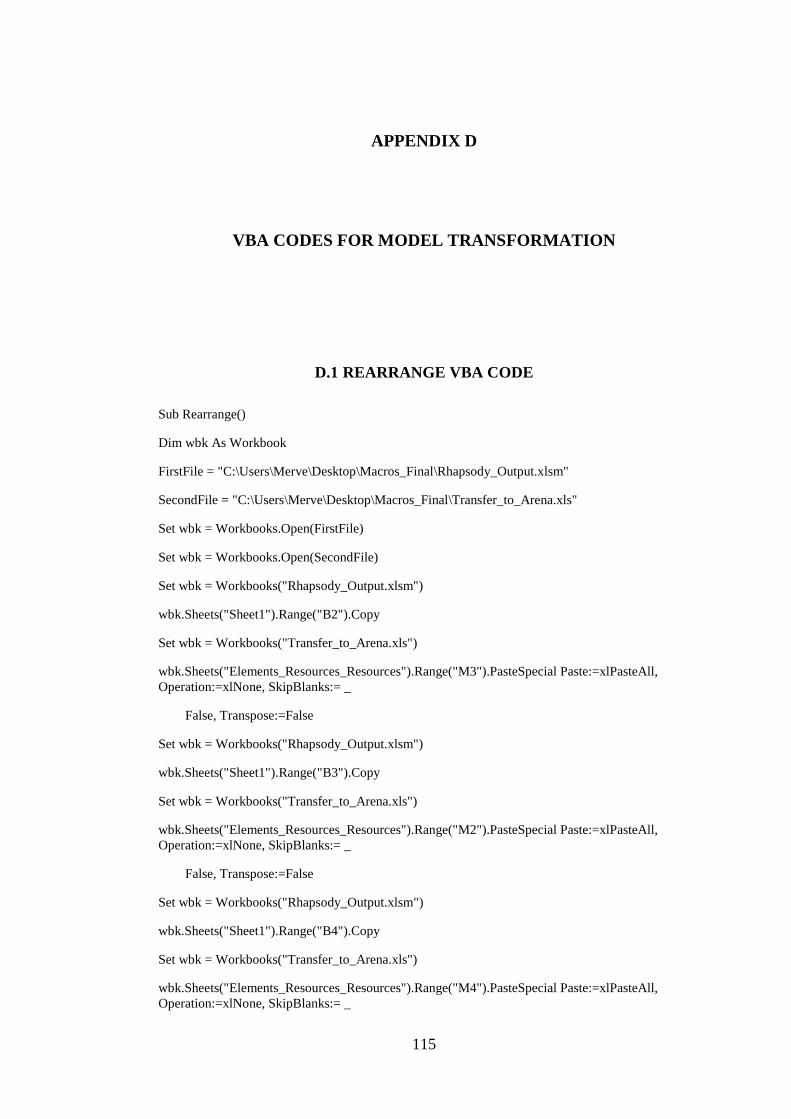
115
APPENDIX D
VBA CODES FOR MODEL TRANSFORMATION
D.1 REARRANGE VBA CODE
Sub Rearrange()
Dim wbk As Workbook
FirstFile = "C:\Users\Merve\Desktop\Macros_Final\Rhapsody_Output.xlsm"
SecondFile = "C:\Users\Merve\Desktop\Macros_Final\Transfer_to_Arena.xls"
Set wbk = Workbooks.Open(FirstFile)
Set wbk = Workbooks.Open(SecondFile)
Set wbk = Workbooks("Rhapsody_Output.xlsm")
wbk.Sheets("Sheet1").Range("B2").Copy
Set wbk = Workbooks("Transfer_to_Arena.xls")
wbk.Sheets("Elements_Resources_Resources").Range("M3").PasteSpecial Paste:=xlPasteAll,
Operation:=xlNone, SkipBlanks:= _
False, Transpose:=False
Set wbk = Workbooks("Rhapsody_Output.xlsm")
wbk.Sheets("Sheet1").Range("B3").Copy
Set wbk = Workbooks("Transfer_to_Arena.xls")
wbk.Sheets("Elements_Resources_Resources").Range("M2").PasteSpecial Paste:=xlPasteAll,
Operation:=xlNone, SkipBlanks:= _
False, Transpose:=False
Set wbk = Workbooks("Rhapsody_Output.xlsm")
wbk.Sheets("Sheet1").Range("B4").Copy
Set wbk = Workbooks("Transfer_to_Arena.xls")
wbk.Sheets("Elements_Resources_Resources").Range("M4").PasteSpecial Paste:=xlPasteAll,
Operation:=xlNone, SkipBlanks:= _

116
False, Transpose:=False
wbk.Save
wbk.Close
Set wbk = Workbooks("Rhapsody_Output.xlsm")
wbk.Sheets("Sheet1").Range("B2:B4").Select
Selection.EntireRow.Delete
Dim objRange As Range
Set objRange = Range("B4:B100")
objRange.TextToColumns _
Destination:=Range("C4"), _
DataType:=xlDelimited, _
TextQualifier:=xlDoubleQuote, _
ConsecutiveDelimiter:=False, _
Tab:=False, _
Semicolon:=False, _
Comma:=False, _
Space:=True, _
Other:=False, _
OtherChar:="-"
Range("B1:B100").Select
Selection.SpecialCells(xlCellTypeBlanks).Select
Selection.EntireRow.Delete
Range("G2").Select
ActiveCell.FormulaR1C1 = _
"=RIGHT(RC[-4],(LEN(RC[-4])-(SEARCH("":"",RC[-4],1))))"
Range("H2").Select
ActiveCell.FormulaR1C1 = _
"=RIGHT(RC[-4],(LEN(RC[-4])-(SEARCH("":"",RC[-4],1))))"
Range("I2").Select
ActiveCell.FormulaR1C1 = _
"=RIGHT(RC[-4],(LEN(RC[-4])-(SEARCH("":"",RC[-4],1))))"
Range("J2").Select

117
ActiveCell.FormulaR1C1 = _
"=RIGHT(RC[-4],(LEN(RC[-4])-(SEARCH("":"",RC[-4],1))))"
Range("G2:J2").Select
Selection.AutoFill Destination:=Range("G2:J58"), Type:=xlFillDefault
Range("G2:J58").Select
Selection.Copy
Selection.PasteSpecial Paste:=xlPasteValues, Operation:=xlNone, SkipBlanks _
:=False, Transpose:=False
Range("C1:F1").Select
Selection.EntireColumn.Delete
Range("C1:F1").Select
Selection.EntireRow.Delete
ActiveWorkbook.SaveAs "C:\Users\Merve\Desktop\Macros_Final\Rhapsody_Output_2.xlsm",
FileFormat:=52
wbk.Close
End Sub

118
D.2 MACRO TRANSFER 1 VBA CODE
Sub COPYCELL()
Dim wbk As Workbook
StrSecondFile = "C:\Users\Merve\Desktop\Macros_Final\Rhapsody_Output_2.xlsm"
StrThirdFile = "C:\Users\Merve\Desktop\Macros_Final\Transfer_to_Arena.xls"
Set wbk = Workbooks.Open(StrSecondFile)
wbk.Sheets("Sheet1").Range("A1:F6").Copy
wbk.Sheets("Sheet1").Range("H1:M6").PasteSpecial Paste:=xlPasteAll, Operation:=xlNone,
SkipBlanks:= _
False, Transpose:=False
wbk.Sheets("Sheet1").Range("A10:F11").Copy
wbk.Sheets("Sheet1").Range("H7:M8").PasteSpecial Paste:=xlPasteAll, Operation:=xlNone,
SkipBlanks:= _
False, Transpose:=False
wbk.Sheets("Sheet1").Range("A7:F9").Copy
wbk.Sheets("Sheet1").Range("H9:M11").PasteSpecial Paste:=xlPasteAll, Operation:=xlNone,
SkipBlanks:= _
False, Transpose:=False
wbk.Sheets("Sheet1").Range("A12:F16").Copy
wbk.Sheets("Sheet1").Range("H12:M16").PasteSpecial Paste:=xlPasteAll, Operation:=xlNone,
SkipBlanks:= _
False, Transpose:=False
wbk.Sheets("Sheet1").Range("A19:F37").Copy
wbk.Sheets("Sheet1").Range("H17:M35").PasteSpecial Paste:=xlPasteAll, Operation:=xlNone,
SkipBlanks:= _
False, Transpose:=False
wbk.Sheets("Sheet1").Range("A17:F18").Copy
wbk.Sheets("Sheet1").Range("H36:M37").PasteSpecial Paste:=xlPasteAll, Operation:=xlNone,
SkipBlanks:= _
False, Transpose:=False
wbk.Sheets("Sheet1").Range("A38:F43").Copy
wbk.Sheets("Sheet1").Range("H38:M43").PasteSpecial Paste:=xlPasteAll, Operation:=xlNone,
SkipBlanks:= _
False, Transpose:=False
wbk.Sheets("Sheet1").Range("A45:F45").Copy

119
wbk.Sheets("Sheet1").Range("H44:M44").PasteSpecial Paste:=xlPasteAll, Operation:=xlNone,
SkipBlanks:= _
False, Transpose:=False
wbk.Sheets("Sheet1").Range("A44:F44").Copy
wbk.Sheets("Sheet1").Range("H45:M45").PasteSpecial Paste:=xlPasteAll, Operation:=xlNone,
SkipBlanks:= _
False, Transpose:=False
wbk.Sheets("Sheet1").Range("A46:F48").Copy
wbk.Sheets("Sheet1").Range("H46:M48").PasteSpecial Paste:=xlPasteAll, Operation:=xlNone,
SkipBlanks:= _
False, Transpose:=False
wbk.Sheets("Sheet1").Range("A50:F50").Copy
wbk.Sheets("Sheet1").Range("H49:M49").PasteSpecial Paste:=xlPasteAll, Operation:=xlNone,
SkipBlanks:= _
False, Transpose:=False
wbk.Sheets("Sheet1").Range("A49:F49").Copy
wbk.Sheets("Sheet1").Range("H50:M50").PasteSpecial Paste:=xlPasteAll, Operation:=xlNone,
SkipBlanks:= _
False, Transpose:=False
wbk.Sheets("Sheet1").Range("A51:F57").Copy
wbk.Sheets("Sheet1").Range("H51:M57").PasteSpecial Paste:=xlPasteAll, Operation:=xlNone,
SkipBlanks:= _
False, Transpose:=False
wbk.Sheets("Sheet1").Range("A1:G1").Select
Selection.EntireColumn.Delete
wbk.Sheets("Sheet1").Range("C1:C57").Copy
Set wbk = Workbooks.Open(StrThirdFile)
wbk.Sheets("Blocks_Delay").Range("I2:I58").PasteSpecial Paste:=xlPasteAll, Operation:=xlNone,
SkipBlanks:= _
False, Transpose:=False
Set wbk = Workbooks("Rhapsody_Output_2.xlsm")
wbk.Sheets("Sheet1").Range("D1").Copy
Set wbk = Workbooks("Transfer_to_Arena.xls")
wbk.Sheets("Blocks_Release_Resources").Range("D4").PasteSpecial Paste:=xlPasteAll,
Operation:=xlNone, SkipBlanks:= _
False, Transpose:=False

120
…*
wbk.Save
wbk.Close
Set wbk = Workbooks("Rhapsody_Output_2.xlsm")
wbk.Save
wbk.Close
End Sub
* Here, VBA code continues with copying resources to be released from
“Rhapsody_Output_2.xlsm” and pastes them to "Transfer_to_Arena.xls".
This part is not included since it is the extension of the above part with no
difference in represented functionality.

121
D.3 MACRO TRANSFER 2 VBA CODE
Sub COPYCELL2()
Dim wbk As Workbook
StrSecondFile = "C:\Users\Merve\Desktop\Macros_Final\Rhapsody_Output_2.xlsm"
StrThirdFile = "C:\Users\Merve\Desktop\Macros_Final\Transfer_to_Arena.xls"
Set wbk = Workbooks.Open(StrSecondFile)
Set wbk = Workbooks.Open(StrThirdFile)
Set wbk = Workbooks("Rhapsody_Output_2.xlsm")
wbk.Sheets("Sheet1").Range("D1").Copy
Set wbk = Workbooks("Transfer_to_Arena.xls")
wbk.Sheets("Blocks_Seize_Resources").Range("D4").PasteSpecial Paste:=xlPasteAll,
Operation:=xlNone, SkipBlanks:= _
False, Transpose:=False
…*
wbk.Save
wbk.Close
Set wbk = Workbooks("Rhapsody_Output_2.xlsm")
wbk.Save
wbk.Close
End Sub
* Here, VBA code continues with copying resources to be seized from
“Rhapsody_Output_2.xlsm” and pastes them to "Transfer_to_Arena.xls".
This part is not included since it is the extension of the above part with no
difference in represented functionality.

122
APPENDIX E
ACTIVITY RESOURCE REQUIREMENTS AND DURATIONS
FOR CASES
Tab
le E
.1A
ctiv
ity R
eso
urc
e R
equ
irem
ents
an
d D
ura
tion
s fo
r D
eter
min
isti
c C
ase
s

123
Table E.1 Activity Resource Requirements and Durations for Deterministic Cases (Continued)
Case D1: Small Scale and Low
Resource Availability
Case D2: Large Scale and Low
Resource Availability
Case D3: Large Scale and High
Resource Availability
Resources Required
Constant
Duration
(Work Day)
Resources Required
Constant
Duration
(Work
Day)
Resources Required
Constant
Duration
(Work Day) Activity
Code* SysEng SME PM SysEng SME PM SysEng SME PM
SS1 4 10 0 10 4 10 0 20 4 10 0 20
SS2 3 20 0 30 3 20 0 60 3 20 0 60
AD1 5 5 0 7 5 5 0 14 5 5 0 14
AD2 5 15 1 8 5 15 1 16 5 15 1 16
AD3 5 10 0 6 5 10 0 12 5 10 0 12
INT1 3 4 1 5 3 4 1 10 3 4 1 10
INT2 1 5 1 3 1 5 1 6 1 5 1 6
INT3 2 5 0 10 2 5 0 20 2 5 0 20
INT4 2 5 0 5 2 5 0 10 2 5 0 10
INT5 2 5 0 5 2 5 0 10 2 5 0 10
INT6 2 5 0 4 2 5 0 8 2 5 0 8
INT7 2 5 0 5 2 5 0 10 2 5 0 10
VER1 8 5 0 3 8 5 0 6 8 5 0 6
VER2 5 10 0 3 5 10 0 6 5 10 0 6
VER3 5 20 1 10 5 20 1 20 5 20 1 20
VER4 5 5 1 4 5 5 1 8 5 5 1 8
VAL1 5 3 1 5 5 3 1 10 5 3 1 10
VAL2 5 5 0 5 5 5 0 10 5 5 0 10
VAL3 3 5 1 5 3 5 1 10 3 5 1 10

124
Table E.1 Activity Resource Requirements and Durations for Deterministic Cases (Continued)
Case D1: Small Scale and Low
Resource Availability
Case D2: Large Scale and Low
Resource Availability
Case D3: Large Scale and High
Resource Availability
Resources Required Constant
Duration
(Work Day)
Resources Required Constant
Duration
(Work
Day)
Resources Required Constant
Duration
(Work Day) Activity
Code* SysEng SME PM SysEng SME PM SysEng SME PM
VAL4 3 10 0 3 3 10 0 6 3 10 0 6
VAL5 5 10 0 5 5 10 0 10 5 10 0 10
VAL6 3 15 0 2 3 15 0 4 3 15 0 4
VAL7 5 10 1 3 5 10 1 6 5 10 1 6
VAL8 5 5 1 3 5 5 1 6 5 5 1 6
MAINT1 2 3 1 2 2 3 1 4 2 3 1 4
MAINT2 2 5 1 3 2 5 1 6 2 5 1 6
MAINT3 1 3 1 5 1 3 1 10 1 3 1 10
MAINT4 0 5 0 3 0 5 0 6 0 5 0 6
MAINT5 0 5 0 5 0 5 0 10 0 5 0 10
MAINT6 0 10 0 60 0 10 0 120 0 10 0 120
MAINT7 0 10 0 60 0 10 0 120 0 10 0 120
MAINT8 1 3 1 60 1 3 1 120 1 3 1 120
OP1 2 5 0 10 2 5 0 20 2 5 0 20
OP2 2 15 0 5 2 15 0 10 2 15 0 10
OP3 2 15 0 60 2 15 0 120 2 15 0 120
OP4 2 15 0 60 2 15 0 120 2 15 0 120
OP5 2 10 1 60 2 10 1 120 2 10 1 120
DIS1 2 3 1 3 2 3 1 6 2 3 1 6
DIS2 2 3 1 2 2 3 1 4 2 3 1 4
DIS3 2 3 0 2 2 3 0 4 2 3 0 4
DIS4 0 5 0 5 0 5 0 10 0 5 0 10

125
Table E.1 Activity Resource Requirements and Durations for Deterministic Cases (Continued)
Case D1: Small Scale and Low
Resource Availability
Case D2: Large Scale and Low
Resource Availability
Case D3: Large Scale and High
Resource Availability
Resources Required Constant
Duration
(Work Day)
Resources Required Constant
Duration
(Work
Day)
Resources Required Constant
Duration
(Work Day) Activity
Code* SysEng SME PM SysEng SME PM SysEng SME PM
DIS5 0 5 0 5 0 5 0 10 0 5 0 10
DIS6 0 5 0 5 0 5 0 10 0 5 0 10
DIS7 1 3 0 5 1 3 0 10 1 3 0 10
SEP1 3 2 1 5 3 2 1 10 3 2 1 10
SEP2 3 2 1 20 3 2 1 40 3 2 1 40
*Shaded activities are high risk, others are low risk activities.

126
Table E.2 Activity Resource Requirements and Durations for Stochastic Cases
Case S1: Small Scale and Low Resource
Availability
Case S2: Large Scale and Low Resource
Availability
Case S3: Large Scale and High Resource
Availability
Small-scale & Low Resource Availability Large-scale & Low Resource Availability Large-scale & High Resource Availability
Activity
Code* SysEng SME PM
Triangular
Duration**
(Work
Day)
SysEng SME PM
Triangular
Duration**
(Work
Day)
SysEng SME PM
Triangular
Duration**
(Work
Day)
SRD1 3 1 1 3, 3, 6 3 1 1 6, 6, 12 3 1 1 6, 6, 12
SRD2 3 1 0 3, 3, 6 3 1 0 6, 6, 12 3 1 0 6, 6, 12
SRD3 4 1 0 4, 4, 8 4 1 0 8, 8, 16 4 1 0 8, 8, 16
MA1 2 1 1 2, 2, 4 2 1 1 4, 4, 8 2 1 1 4, 4, 8
MA2 2 1 1 3, 3, 6 2 1 1 6, 6, 12 2 1 1 6, 6, 12
MA3 2 1 0 2, 2, 4 2 1 0 4, 4, 8 2 1 0 4, 4, 8
RA3 3 1 1 3, 3, 6 3 1 1 6, 6, 12 3 1 1 6, 6, 12
RA4 4 2 0 7, 7, 14 4 2 0 14, 14, 28 4 2 0 14, 14, 28
RA5 3 2 0 5, 5, 10 3 2 0 10, 10, 20 3 2 0 10, 10, 20
FA1 4 5 1 8, 8, 16 4 5 1 16, 16, 32 4 5 1 16, 16, 32
FA2 6 5 0 7, 7, 14 6 5 0 14, 14, 28 6 5 0 14, 14, 28
SS1 4 10 0 10, 10, 20 4 10 0 20, 20, 40 4 10 0 20, 20, 40
SS2 3 20 0 30, 30, 60 3 20 0 60, 60, 120 3 20 0 60, 60, 120

127
Table E.2 Activity Resource Requirements and Durations for Stochastic Cases (Continued)
Case S1: Small Scale and Low Resource
Availability
Case S2: Large Scale and Low Resource
Availability
Case S3: Large Scale and High Resource
Availability
Small-scale & Low Resource Availability Large-scale & Low Resource Availability Large-scale & High Resource Availability
Activity
Code* SysEng SME PM
Triangular
Duration**
(Work
Day)
SysEng SME PM
Triangular
Duration**
(Work
Day)
SysEng SME PM
Triangular
Duration**
(Work
Day)
AD1 5 5 0 7, 7, 14 5 5 0 14, 14, 28 5 5 0 14, 14, 28
AD2 5 15 1 8, 8, 16 5 15 1 16, 16, 32 5 15 1 16, 16, 32
AD3 5 10 0 6, 6, 12 5 10 0 12, 12, 24 5 10 0 12, 12, 24
INT1 3 4 1 5, 5, 7.5 3 4 1 10, 10, 15 3 4 1 10, 10, 15
INT2 1 5 1 3, 3, 4.5 1 5 1 6, 6, 9 1 5 1 6, 6, 9
INT3 2 5 0 10, 10, 15 2 5 0 20, 20, 30 2 5 0 20, 20, 30
INT4 2 5 0 5, 5, 7.5 2 5 0 10, 10, 15 2 5 0 10, 10, 15
INT5 2 5 0 5, 5, 7.5 2 5 0 10, 10, 15 2 5 0 10, 10, 15
INT6 2 5 0 4, 4, 6 2 5 0 8, 8, 12 2 5 0 8, 8, 12
INT7 2 5 0 5, 5, 7.5 2 5 0 10, 10, 15 2 5 0 10, 10, 15
VER1 8 5 0 3, 3, 4.5 8 5 0 6, 6, 9 8 5 0 6, 6, 9
VER2 5 10 0 3, 3, 4.5 5 10 0 6, 6, 9 5 10 0 6, 6, 9
VER3 5 20 1 10, 10, 15 5 20 1 20, 20, 30 5 20 1 20, 20, 30
VER4 5 5 1 4, 4, 6 5 5 1 8, 8, 12 5 5 1 8, 8, 12
VAL1 5 3 1 5, 5, 7.5 5 3 1 10, 10, 15 5 3 1 10, 10, 15
VAL2 5 5 0 5, 5, 7.5 5 5 0 10, 10, 15 5 5 0 10, 10, 15

128
Table E.2 Activity Resource Requirements and Durations for Stochastic Cases (Continued)
Case S1: Small Scale and Low Resource
Availability
Case S2: Large Scale and Low Resource
Availability
Case S3: Large Scale and High Resource
Availability
Small-scale & Low Resource Availability Large-scale & Low Resource Availability Large-scale & High Resource Availability
Activity
Code* SysEng SME PM
Triangular
Duration**
(Work
Day)
SysEng SME PM
Triangular
Duration**
(Work
Day)
SysEng SME PM
Triangular
Duration**
(Work
Day)
VAL3 3 5 1 5, 5, 7.5 3 5 1 10, 10, 15 3 5 1 10, 10, 15
VAL4 3 10 0 3, 3, 4.5 3 10 0 6, 6, 9 3 10 0 6, 6, 9
VAL5 5 10 0 5, 5, 7.5 5 10 0 10, 10, 15 5 10 0 10, 10, 15
VAL6 3 15 0 2, 2, 3 3 15 0 4, 4, 6 3 15 0 4, 4, 6
VAL7 5 10 1 3, 3, 4.5 5 10 1 6, 6, 9 5 10 1 6, 6, 9
VAL8 5 5 1 3, 3, 4.5 5 5 1 6, 6, 9 5 5 1 6, 6, 9
MAINT1 2 3 1 2, 2, 3 2 3 1 4, 4, 6 2 3 1 4, 4, 6
MAINT2 2 5 1 3, 3, 4.5 2 5 1 6, 6, 9 2 5 1 6, 6, 9
MAINT3 1 3 1 5, 5, 7.5 1 3 1 10, 10, 15 1 3 1 10, 10, 15
MAINT4 0 5 0 3, 3, 4.5 0 5 0 6, 6, 9 0 5 0 6, 6, 9
MAINT5 0 5 0 5, 5, 7.5 0 5 0 10, 10, 15 0 5 0 10, 10, 15
MAINT6 0 10 0 60, 60, 90 0 10 0 120, 120,
180 0 10 0
120, 120,
180
MAINT7 0 10 0 60, 60, 90 0 10 0 120, 120,
180 0 10 0
120, 120,
180
MAINT8 1 3 1 60, 60, 90 1 3 1 120, 120,
180 1 3 1
120, 120,
180
OP1 2 5 0 10, 10, 15 2 5 0 20, 20, 30 2 5 0 20, 20, 30

129
Table E.2 Activity Resource Requirements and Durations for Stochastic Cases (Continued)
Case S1: Small Scale and Low Resource
Availability
Case S2: Large Scale and Low Resource
Availability
Case S3: Large Scale and High Resource
Availability
Small-scale & Low Resource Availability Large-scale & Low Resource Availability Large-scale & High Resource Availability
Activity
Code* SysEng SME PM
Triangular
Duration**
(Work
Day)
SysEng SME PM
Triangular
Duration**
(Work
Day)
SysEng SME PM
Triangular
Duration**
(Work
Day)
OP2 2 15 0 5, 5, 7.5 2 15 0 10, 10, 15 2 15 0 10, 10, 15
OP3 2 15 0 60, 60, 90 2 15 0 120, 120,
180 2 15 0
120, 120,
180
OP4 2 15 0 60, 60, 90 2 15 0 120, 120,
180 2 15 0
120, 120,
180
OP5 2 10 1 60, 60, 90 2 10 1 120, 120,
180 2 10 1
120, 120,
180
DIS1 2 3 1 3, 3, 4.5 2 3 1 6, 6, 9 2 3 1 6, 6, 9
DIS2 2 3 1 2, 2, 3 2 3 1 4, 4, 6 2 3 1 4, 4, 6
DIS3 2 3 0 2, 2, 3 2 3 0 4, 4, 6 2 3 0 4, 4, 6
DIS4 0 5 0 5, 5, 7.5 0 5 0 10, 10, 15 0 5 0 10, 10, 15
DIS5 0 5 0 5, 5, 7.5 0 5 0 10, 10, 15 0 5 0 10, 10, 15
DIS6 0 5 0 5, 5, 7.5 0 5 0 10, 10, 15 0 5 0 10, 10, 15
DIS7 1 3 0 5, 5, 7.5 1 3 0 10, 10, 15 1 3 0 10, 10, 15
SEP1 3 2 1 5, 5, 7.5 3 2 1 10, 10, 15 3 2 1 10, 10, 15
SEP2 3 2 1 20, 20, 30 3 2 1 40, 40, 60 3 2 1 40, 40, 60
*Shaded activities are high risk, others are low risk activities.
** Minimum, mode and maximum duration values are given as triangular distribution parameters.

130
APPENDIX F
REPLICATION NUMBER ESTIMATION RESULTS
Tab
le F
.1 R
esu
lts
For
Rep
lica
tion
Nu
mb
er E
stim
ati
on
Alg
ori
thm

131
Table F.1 Results For Replication Number Estimation Algorithm (Continued)
CASE S1 CASE S2 CASE S3
Parameter
Definition
Project
Duration
SysEng
Utilization
(%)
SME
Utilization
(%)
PM
Utilization
(%)
Project
Duration
SysEng
Utilization
(%)
SME
Utilization
(%)
PM
Utilization
(%)
Project
Duration
SysEng
Utilization
(%)
SME
Utilization
(%)
PM
Utilization
(%)
Sample mean
(Ῡ) 455.3 34.8 51.7 29.4 910.7 34.8 51.7 29.4 758.3 21.0 31.0 17.9
Sample
variance (s2) 94.8 0.3 0.5 0.8 379.5 0.3 0.5 0.8 501.2 0.2 1.0 0.6
Sample
standard
deviation (s) 9.7 0.5 0.7 0.9 19.5 0.5 0.7 0.9 22.4 0.4 1.0 0.8
Significance
level (α) 0.1 0.1 0.1 0.1 0.1 0.1 0.1 0.1 0.1 0.1 0.1 0.1
Student-t
distribution
value
(t n-1, 1-α/2) 1.8 1.8 1.8 1.8 1.8 1.8 1.8 1.8 1.8 1.8 1.8 1.8
CI half
length (h) 5.6 0.3 0.4 0.5 11.3 0.3 0.4 0.5 13.0 0.2 0.6 0.5
Relative
precision (r) 0.1 0.1 0.1 0.1 0.1 0.1 0.1 0.1 0.1 0.1 0.1 0.1
Desired CI
half length
(h*) 45.5 3.5 5.2 2.9 91.1 3.5 5.2 2.9 75.8 2.1 3.1 1.8
h≤h* check YES YES YES YES YES YES YES YES YES YES YES YES
Variance (σ2) 9.5 0.0 0.0 0.1 37.9 0.0 0.0 0.1 50.1 0.0 0.1 0.1

132
Table F.1 Results For Replication Number Estimation Algorithm (Continued)
CASE S1 CASE S2 CASE S3
Parameter
Definition
Project
Duration
SysEng
Utilization
(%)
SME
Utilization
(%)
PM
Utilization
(%)
Project
Duration
SysEng
Utilization
(%)
SME
Utilization
(%)
PM
Utilization
(%)
Project
Duration
SysEng
Utilization
(%)
SME
Utilization
(%)
PM
Utilization
(%)
Standard
Deviation (σ) 3.1 0.2 0.2 0.3 6.2 0.2 0.2 0.3 7.1 0.1 0.3 0.2
CI Lower
Limit 449.7 34.5 51.3 28.9 899.4 34.5 51.3 28.9 745.3 20.7 30.5 17.5
CI Upper
Limit 461.0 35.2 52.1 29.9 922.0 35.2 52.1 29.9 771.3 21.2 31.6 18.4


![[Luyben] Process Modeling Simulation and Control for Chemical Engineers](https://static.fdocuments.us/doc/165x107/545be701b1af9f131f8b46e9/luyben-process-modeling-simulation-and-control-for-chemical-engineers.jpg)