Overview of the Simulation Modeling Process of the Simulation Modeling Process Nathaniel Osgood ......

Overview of the Simulation Modeling Process

Nathaniel Osgood

CMPT 858

January 18, 2011

Announcements

• Tutorial vote link sent

– Please vote by Wednesday evening

• Download & install Vensim PLE

– http://www.vensim.com/freedownload.html

http://www.vensim.com/freedownload.html

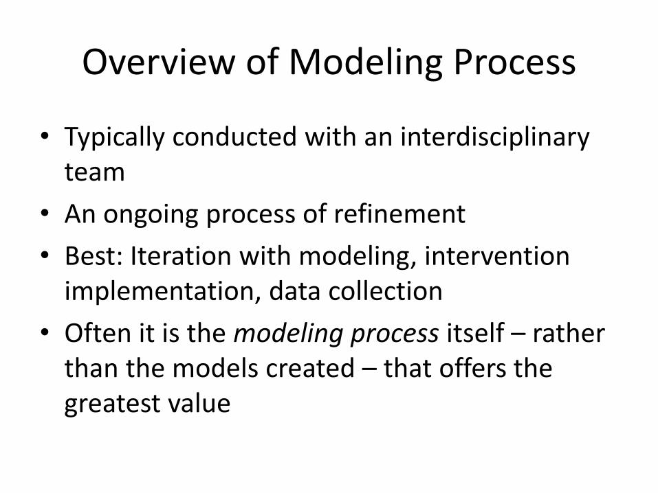
Overview of Modeling Process

• Typically conducted with an interdisciplinary team

• An ongoing process of refinement

• Best: Iteration with modeling, intervention implementation, data collection

• Often it is the modeling process itself – rather than the models created – that offers the greatest value

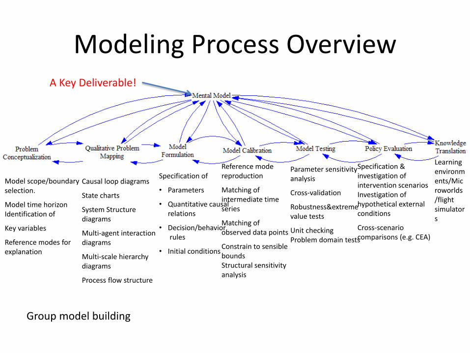
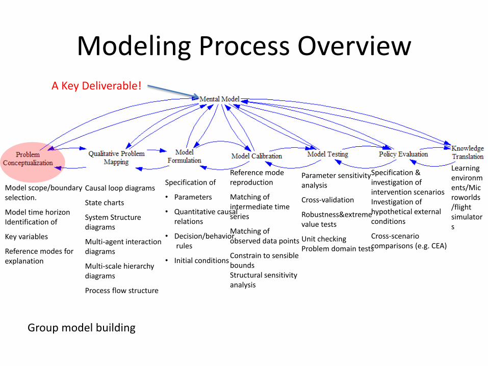
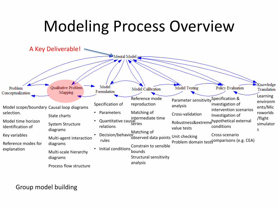
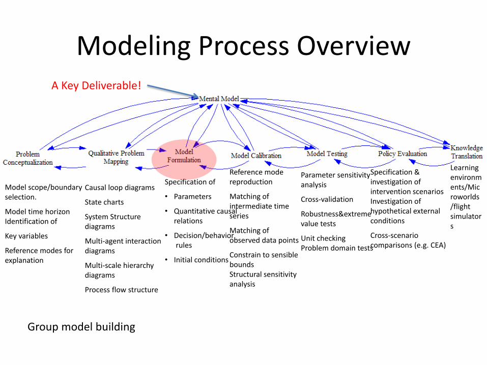
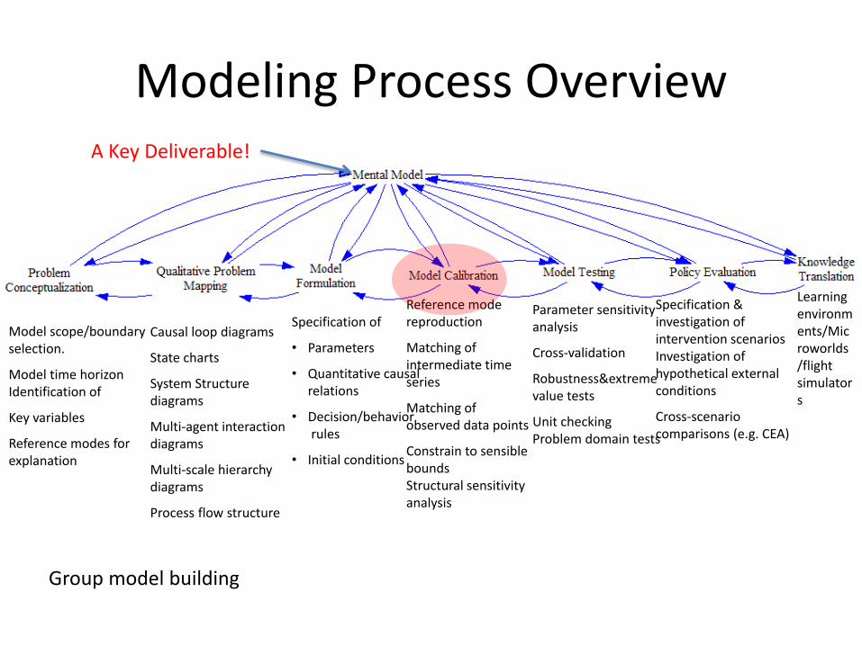
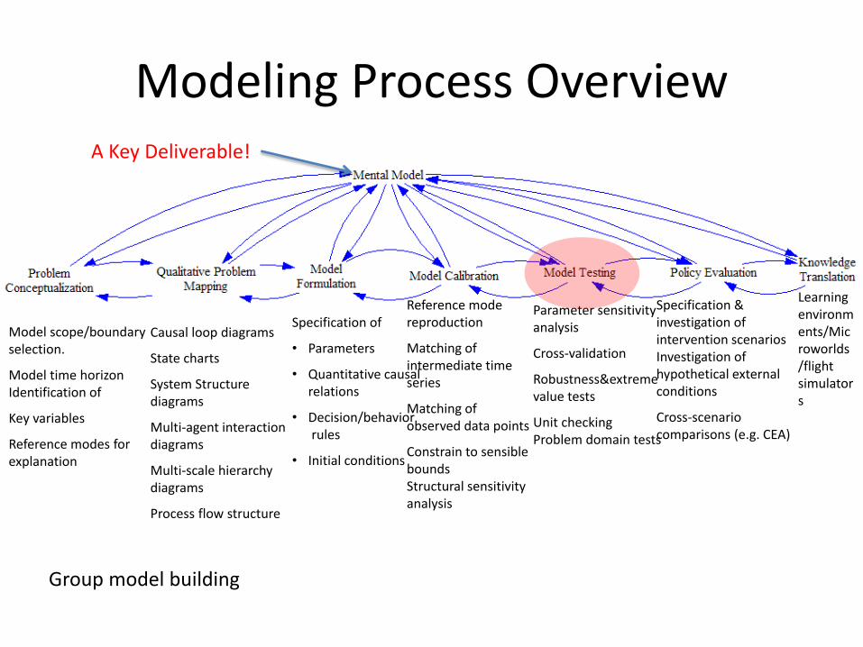
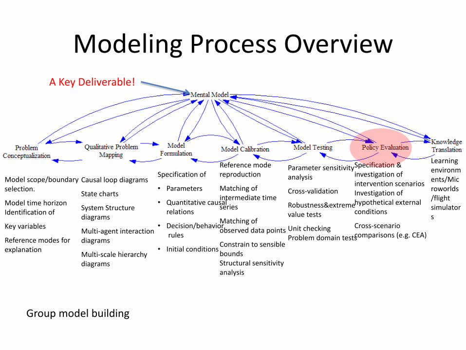
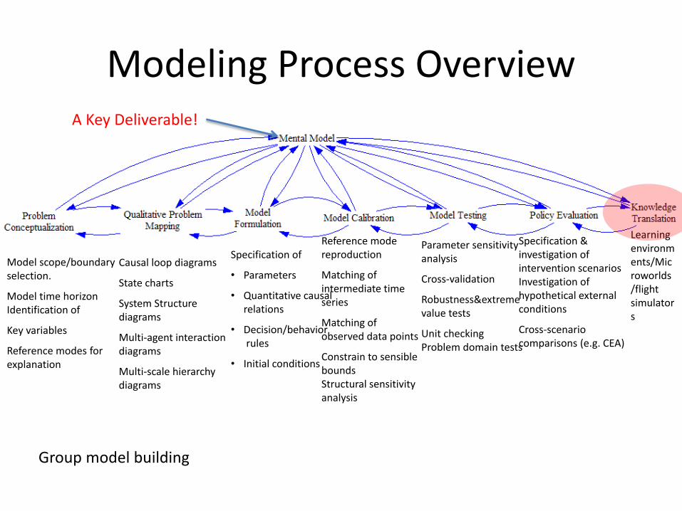
Modeling Process Overview

A Key Deliverable!

Model scope/boundary selection.

Model time horizon Identification of

Key variables

Reference modes for explanation

Causal loop diagrams

State charts

System Structure diagrams

Multi-agent interaction diagrams

Multi-scale hierarchy diagrams

Process flow structure

Specification of

• Parameters

• Quantitative causal relations

• Decision/behavior rules

• Initial conditions

Reference mode reproduction

Matching of intermediate time series

Matching of observed data points

Constrain to sensible bounds Structural sensitivity analysis

Specification & investigation of intervention scenarios Investigation of hypothetical external conditions

Cross-scenario comparisons (e.g. CEA)

Parameter sensitivity analysis

Cross-validation

Robustness&extreme value tests

Unit checking Problem domain tests

Learning environments/Microworlds/flight simulators

Group model building

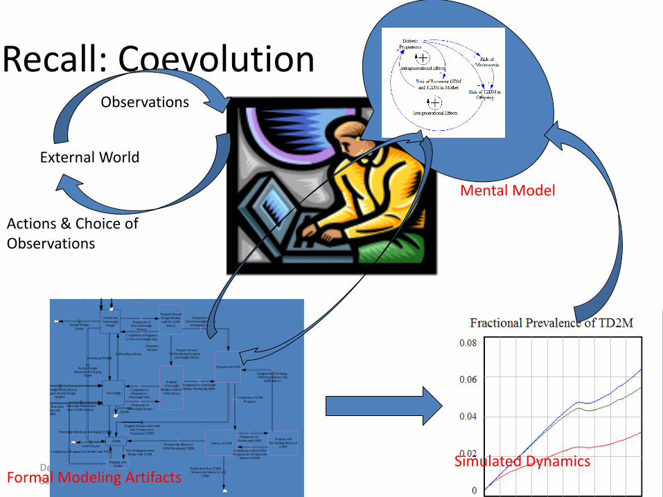
Recall: Coevolution

Department of Computer Science

Normal and

Underweight

Weight

Overweight

Pregnant with GDM

History of GDMT2DM

Developing Obesity

Pregnant Normal

Weight Mothers

with No GDM

History

Completion of Pregnancy

to Non-Overweight State

Completion of GDM

Pregnancy

Women with History of

GDM Developing T2DM

Overweight Individuals Developing T2DM

Normal WeightIndividuals Developing

T2DM

Pregnant with

T2DM

New Pregnancies from

Mother with T2DMCompletion of Pregnancy for Mother with T2DM

Pregnant

Overweight

Mothers with No

GDM History

Pregnancies of

Overweight Women

Completion ofPregnancy to

Overweight State

Pregnancies ofNon-Overweight

Women

Pregnancies to Overweight

Mother Developing GDM

Pregnancies toNon-Overweight Mother

Developing GDM

Pregnant with

Pre-Existing History of

GDM

Pregnancies for

Women with GDM

Pregnancies DevelopingGDM from Mother with

GDM History

Completion of Non-GDMPregnancy for Woman with

History of GDM

Shedding Obesity

Pregnant WomenDeveloping PersistentOverweight/Obesity

Oveweight Babies Born

from T2DM Mothers

Pregnant Women with GDMthat Continue on toPostpartum T2DM

Normal Weight Babies Bornfrom Non-GDM Mother with

History of GDM

Overweight Babies Born fromNon-GDM Mother with

History of GDM

Normal Weight BabiesBorn from GDM

Pregnancy

Overweight Babies Born

from GDM Pregnancy

Overweight Babies Born toPregnant Normal Weight

Mothers

Overweight Babies Bornfrom Pregnant Overweight

Mothers

Normal Weight Babies Born to

Mothers without GDM

Normal Weight BabiesBorn from T2DM

Pregnancy

Pregnancy

Duration

<Birth Rate>

Normal Weight Babies Bornto Overweight Mothers

without GDM

Normal Weight

Deaths

Overweight

Deaths

T2DM Deaths

Deaths from Non-T2DMWomen with History of

GDMFormal Modeling Artifacts Simulated Dynamics

Mental Model

External World

Actions & Choice of Observations

Observations


A Key Deliverable!



Key variables



State charts





Specification of

• Parameters











Cross-validation





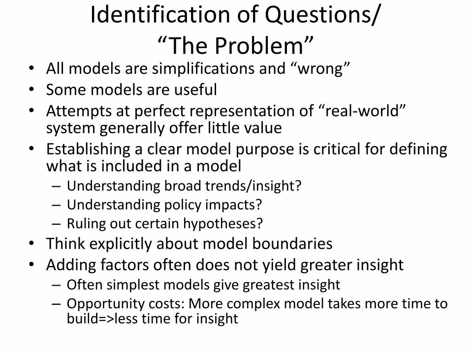
Identification of Questions/ “The Problem”

• All models are simplifications and “wrong” • Some models are useful • Attempts at perfect representation of “real-world”

system generally offer little value • Establishing a clear model purpose is critical for defining

what is included in a model – Understanding broad trends/insight? – Understanding policy impacts? – Ruling out certain hypotheses?

• Think explicitly about model boundaries • Adding factors often does not yield greater insight

– Often simplest models give greatest insight – Opportunity costs: More complex model takes more time to

build=>less time for insight

Importance of Purpose

Firmness of purpose is one of the most necessary sinews of character, and one of the best instruments of success. Without it genius wastes its efforts in a maze of inconsistencies.

Lord Chesterfield

The secret of success is constancy of purpose.

Benjamin Disraeli

The art of model building is knowing what to cut out, and the purpose of the model acts as the logical knife. It provides the criterion about what will be cut, so that only the essential features necessary to fulfill the purpose are left.

John Sterman

H Taylor, 2001

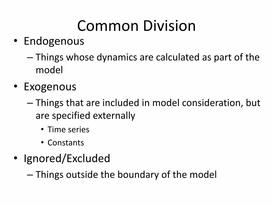
Common Division • Endogenous

– Things whose dynamics are calculated as part of the model

• Exogenous

– Things that are included in model consideration, but are specified externally

• Time series

• Constants

• Ignored/Excluded

– Things outside the boundary of the model

Example of Boundary Definition

(1998)


A Key Deliverable!



Key variables



State charts





Specification of

• Parameters











Cross-validation





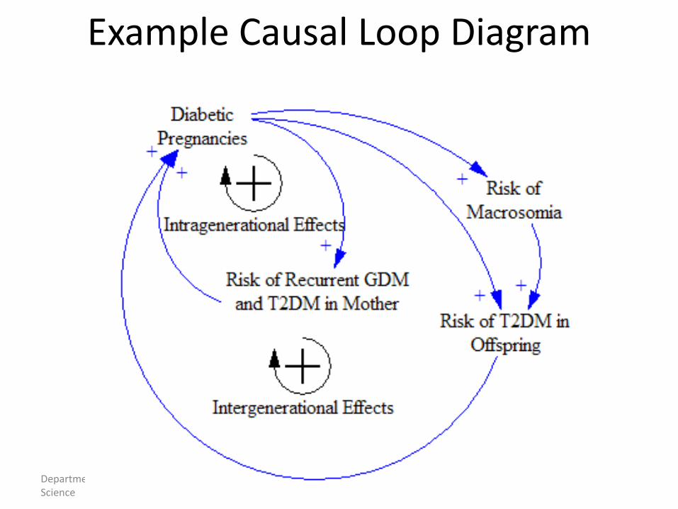
Example Causal Loop Diagram


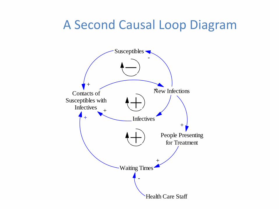
A Second Causal Loop Diagram

Infectives

New Infections

People Presenting

for Treatment

Waiting Times

+

+

Health Care Staff

-

Susceptibles-

Contacts ofSusceptibles with

Infectives

++

++

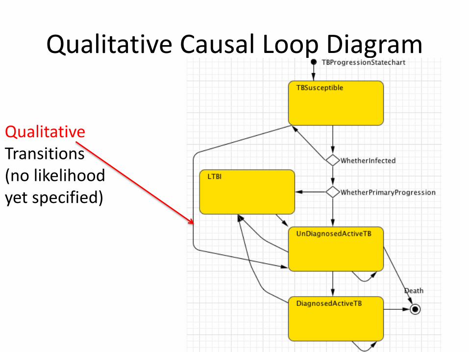
Qualitative Causal Loop Diagram

Qualitative Transitions (no likelihood yet specified)

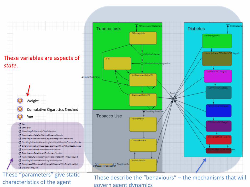
These “parameters” give static characteristics of the agent

These describe the “behaviours” – the mechanisms that will govern agent dynamics

Age

Cumulative Cigarettes Smoked

Weight

These variables are aspects of state.

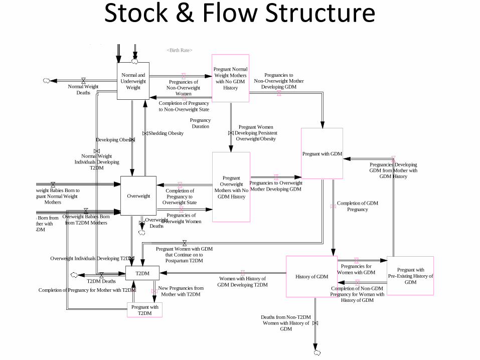
Stock & Flow Structure

Normal and

Underweight

Weight

Overweight

Pregnant with GDM

History of GDMT2DM

Developing Obesity

Pregnant Normal

Weight Mothers

with No GDM

History

Completion of Pregnancy

to Non-Overweight State

Completion of GDM

Pregnancy

Women with History of

GDM Developing T2DM

Overweight Individuals Developing T2DM

Normal WeightIndividuals Developing

T2DM

Pregnant with

T2DM

New Pregnancies from

Mother with T2DMCompletion of Pregnancy for Mother with T2DM

Pregnant

Overweight

Mothers with No

GDM History

Pregnancies of

Overweight Women

Completion ofPregnancy to

Overweight State

Pregnancies ofNon-Overweight

Women

Pregnancies to Overweight

Mother Developing GDM

Pregnancies toNon-Overweight Mother

Developing GDM

Pregnant with

Pre-Existing History of

GDM

Pregnancies for

Women with GDM

Pregnancies DevelopingGDM from Mother with

GDM History

Completion of Non-GDMPregnancy for Woman with

History of GDM

Shedding Obesity

Pregnant WomenDeveloping PersistentOverweight/Obesity

Oveweight Babies Born

from T2DM Mothers

Pregnant Women with GDMthat Continue on toPostpartum T2DM

Normal Weight Babies Bornfrom Non-GDM Mother with

History of GDM

Overweight Babies Born fromNon-GDM Mother with

History of GDM

Normal Weight BabiesBorn from GDM

Pregnancy

Overweight Babies Born

from GDM Pregnancy

Overweight Babies Born toPregnant Normal Weight

Mothers

Overweight Babies Bornfrom Pregnant Overweight

Mothers

Normal Weight Babies Born to

Mothers without GDM

Normal Weight BabiesBorn from T2DM

Pregnancy

Pregnancy

Duration

<Birth Rate>

Normal Weight Babies Bornto Overweight Mothers

without GDM

Normal Weight

Deaths

Overweight

Deaths

T2DM Deaths

Deaths from Non-T2DMWomen with History of

GDM

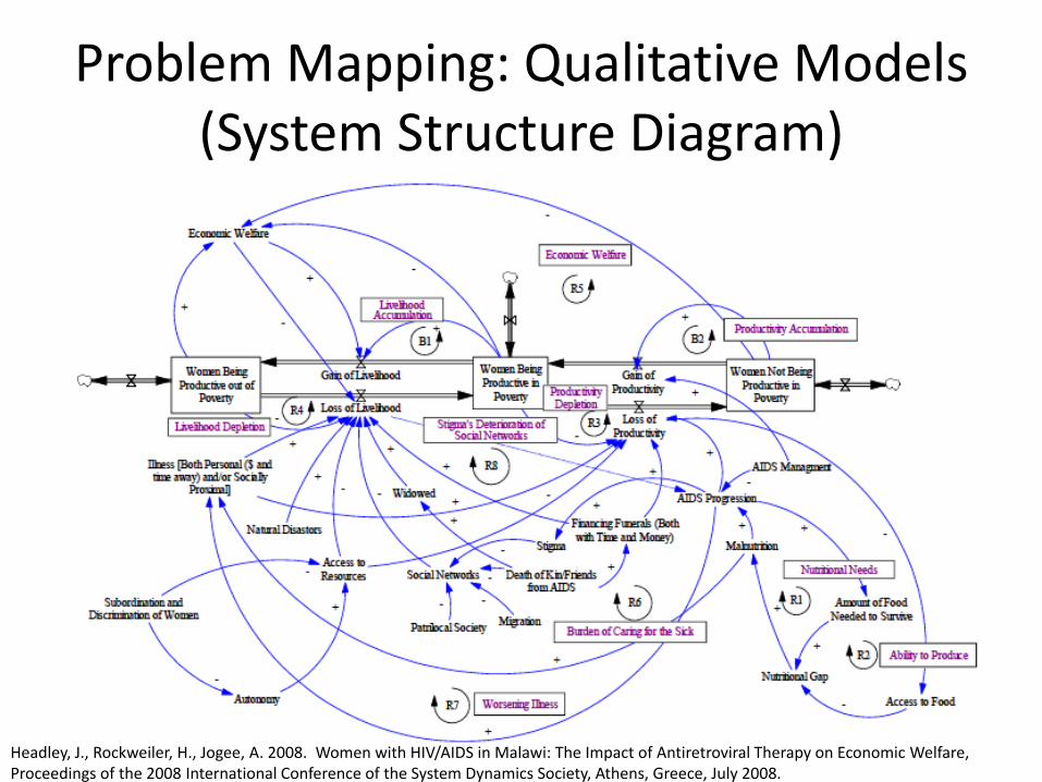
Problem Mapping: Qualitative Models (System Structure Diagram)

Headley, J., Rockweiler, H., Jogee, A. 2008. Women with HIV/AIDS in Malawi: The Impact of Antiretroviral Therapy on Economic Welfare, Proceedings of the 2008 International Conference of the System Dynamics Society, Athens, Greece, July 2008.


A Key Deliverable!



Key variables



State charts





Specification of

• Parameters











Cross-validation





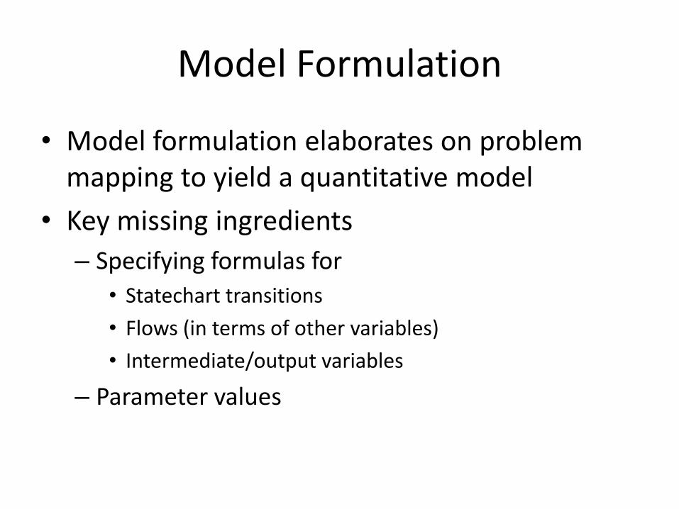
Model Formulation

• Model formulation elaborates on problem mapping to yield a quantitative model

• Key missing ingredients

– Specifying formulas for

• Statechart transitions

• Flows (in terms of other variables)

• Intermediate/output variables

– Parameter values

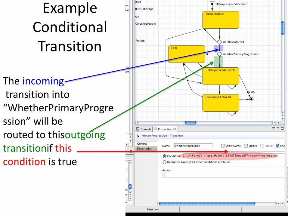
Example Conditional Transition

The incoming transition into “WhetherPrimaryProgression” will be routed to thisoutgoing transitionif this condition is true

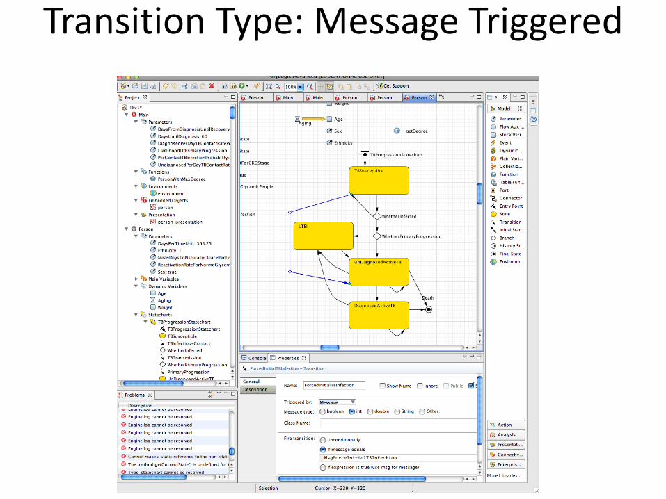
Transition Type: Message Triggered

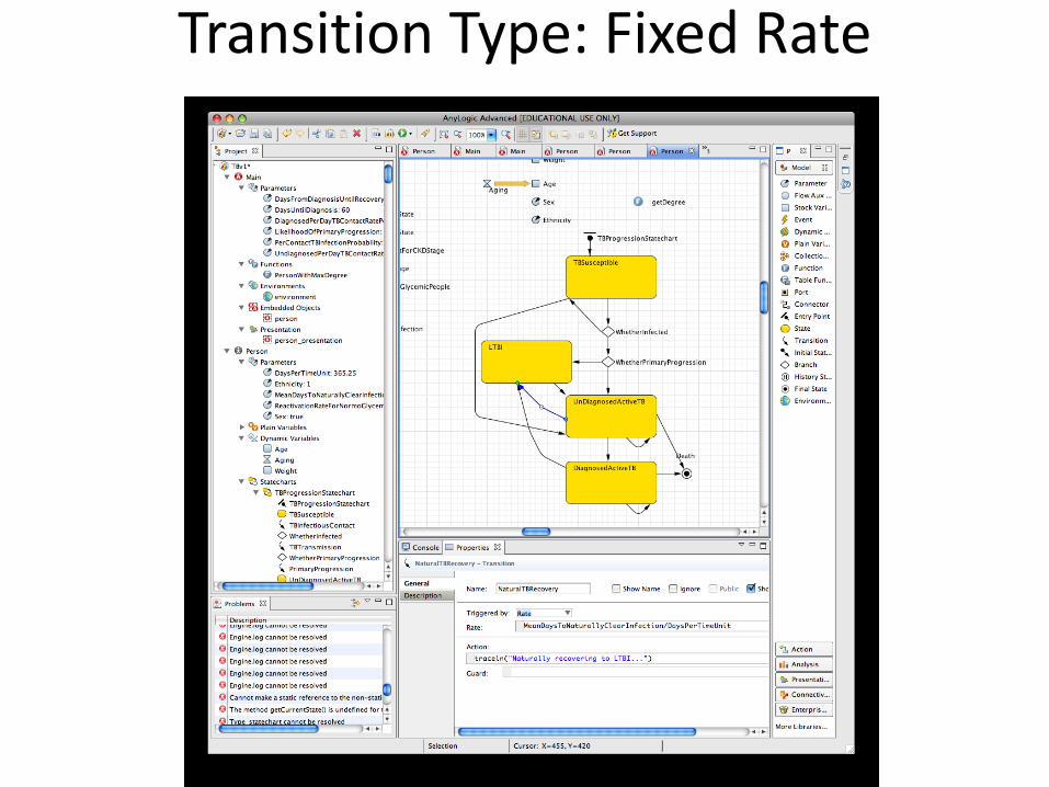
Transition Type: Fixed Rate

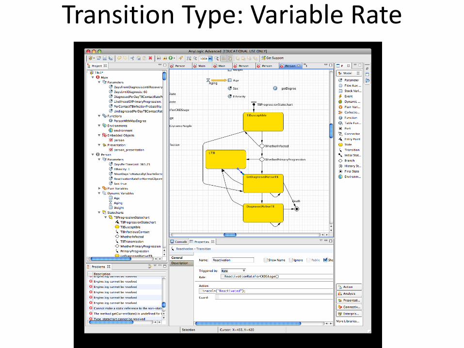
Transition Type: Variable Rate

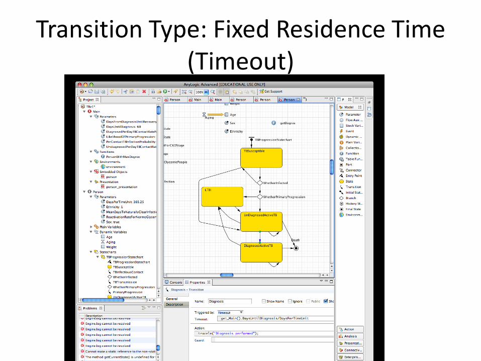
Transition Type: Fixed Residence Time (Timeout)

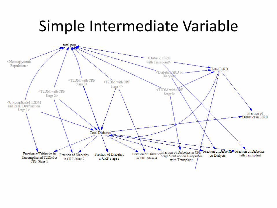
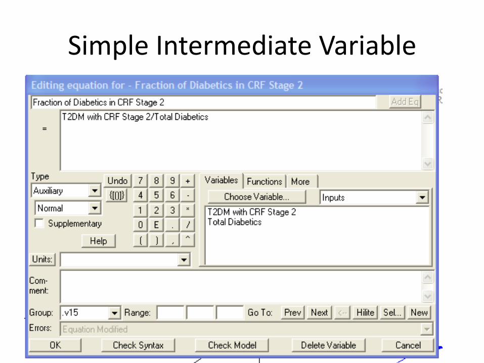
Simple Intermediate Variable

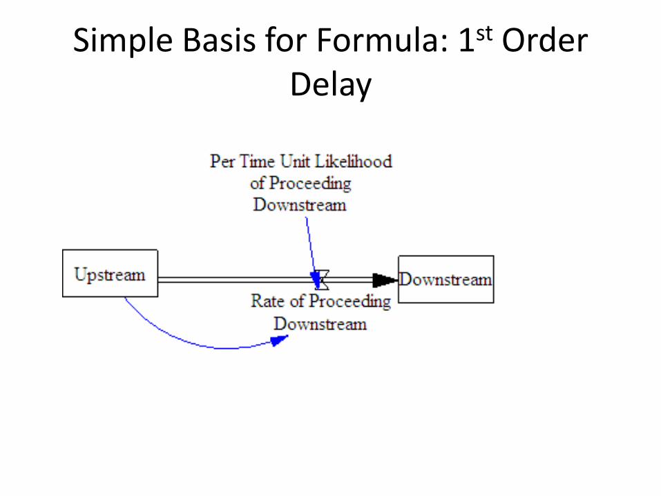
Simple Basis for Formula: 1st Order Delay

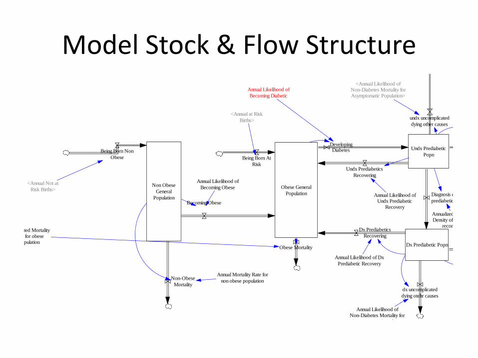
Model Stock & Flow Structure

Non Obese

General

Population

Undx Prediabetic

Popn

Obese General

Population

Becoming Obese

Dx Prediabetic Popn

DevelopingDiabetesBeing Born Non

Obese Being Born At

Risk

Annual Likelihood of

Becoming Obese


Becoming Diabetic

Diagnosis of

prediabetics

undx uncomplicated

dying other causes

dx uncomplicated

dying otehr causes

Annualized ProbabilityDensity of prediabetic

recongnition

Non-Obese

Mortality

Annual Mortality Rate for

non obese population

Annualized MortalityRate for obese

population

<Annual Not at

Risk Births>

Annual Likelihood ofNon-Diabetes Mortality forAsymptomatic Population

<Annual at Risk

Births>

Obese Mortality

Dx Prediabetics

Recovering

Undx Prediabetics

Recovering

Annual Likelihood ofUndx Prediabetic

Recovery

Annual Likelihood of Dx

Prediabetic Recovery

<Annual Likelihood ofNon-Diabetes Mortality forAsymptomatic Population>

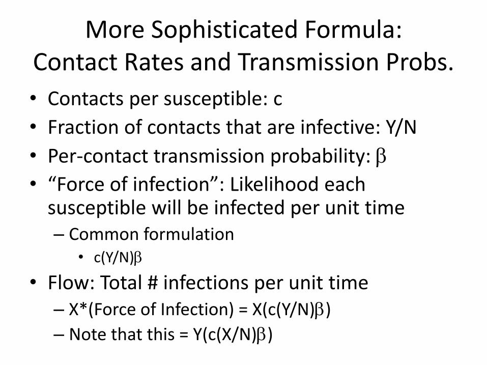
More Sophisticated Formula: Contact Rates and Transmission Probs.

• Contacts per susceptible: c

• Fraction of contacts that are infective: Y/N

• Per-contact transmission probability:

• “Force of infection”: Likelihood each susceptible will be infected per unit time – Common formulation

• c(Y/N)

• Flow: Total # infections per unit time – X*(Force of Infection) = X(c(Y/N))

– Note that this = Y(c(X/N))

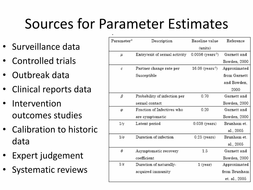
Sources for Parameter Estimates

• Surveillance data

• Controlled trials

• Outbreak data

• Clinical reports data

• Intervention outcomes studies

• Calibration to historic data

• Expert judgement

• Systematic reviews

Anderson & May

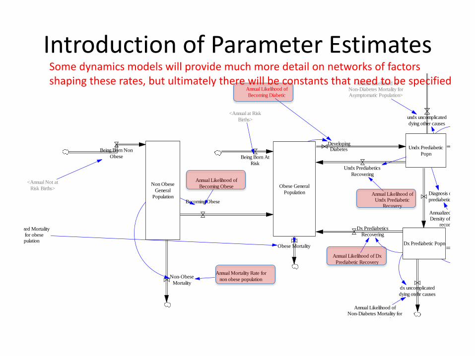
Introduction of Parameter Estimates

Non Obese

General

Population

Undx Prediabetic

Popn

Obese General

Population

Becoming Obese

Dx Prediabetic Popn

DevelopingDiabetesBeing Born Non

Obese Being Born At

Risk


Becoming Obese


Becoming Diabetic

Diagnosis of

prediabetics

undx uncomplicated

dying other causes

dx uncomplicated

dying otehr causes

Annualized ProbabilityDensity of prediabetic

recongnition

Non-Obese

Mortality

Annual Mortality Rate for

non obese population

Annualized MortalityRate for obese

population

<Annual Not at

Risk Births>

Annual Likelihood ofNon-Diabetes Mortality forAsymptomatic Population

<Annual at Risk

Births>

Obese Mortality

Dx Prediabetics

Recovering

Undx Prediabetics

Recovering

Annual Likelihood ofUndx Prediabetic

Recovery

Annual Likelihood of Dx

Prediabetic Recovery

<Annual Likelihood ofNon-Diabetes Mortality forAsymptomatic Population>

Some dynamics models will provide much more detail on networks of factors shaping these rates, but ultimately there will be constants that need to be specified


A Key Deliverable!



Key variables



State charts





Specification of

• Parameters











Cross-validation





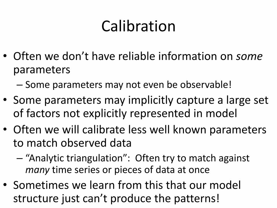
Calibration

• Often we don’t have reliable information on some parameters – Some parameters may not even be observable!

• Some parameters may implicitly capture a large set of factors not explicitly represented in model

• Often we will calibrate less well known parameters to match observed data – “Analytic triangulation”: Often try to match against

many time series or pieces of data at once

• Sometimes we learn from this that our model structure just can’t produce the patterns!

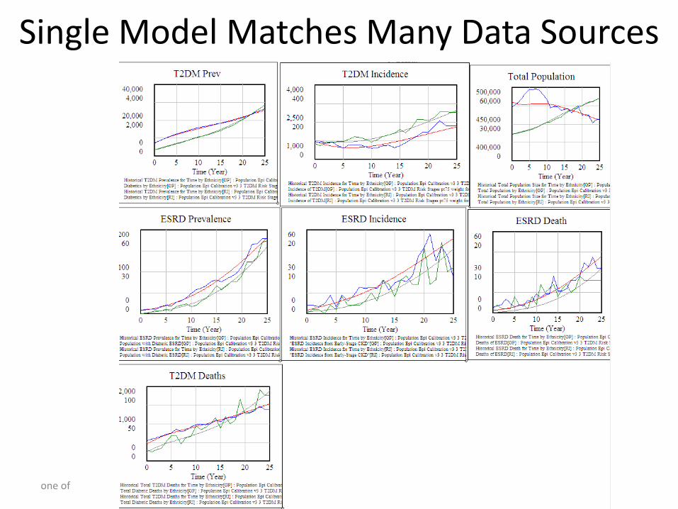
Single Model Matches Many Data Sources

one of

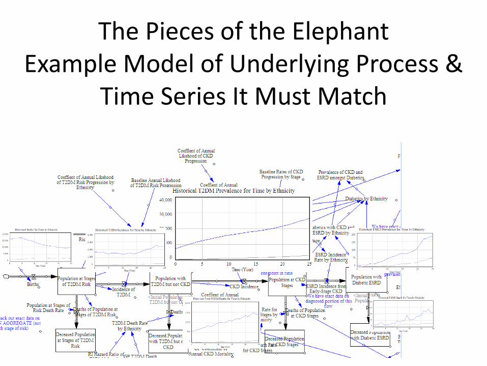
The Pieces of the Elephant Example Model of Underlying Process &

Time Series It Must Match


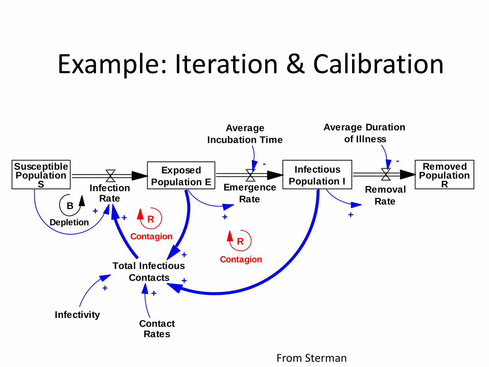
SusceptiblePopulation

S

B

Exposed

Population E

Depletion

Infectious

Population IEmergence

Rate

RemovedPopulation

RRemoval

Rate

Average

Incubation Time

-

+ +

Average Duration

of Illness

Total Infectious

Contacts

ContactRates

Infectivity

++

+

+

R

ContagionR

Contagion

InfectionRate

++

-

Adapted from Sterman

Example: Iteration & Calibration

From Sterman

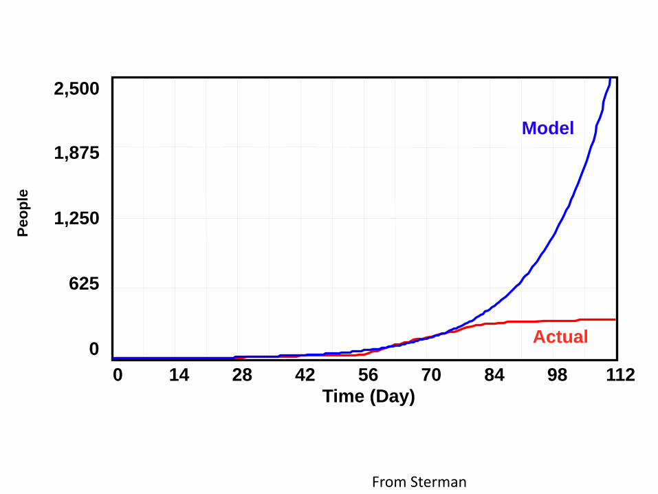
SEIR Model vs. Data, Taiwan Cumulative Cases, No Behavioral Response

2,500

1,875

1,250

625

0

0 14 28 42 56 70 84 98 112 Time (Day)

Pe

op

le

Model

Actual

Adapted from Sterman From Sterman

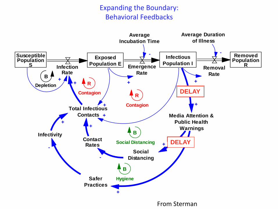
Expanding the Boundary: Behavioral Feedbacks

SusceptiblePopulation

S

B

Exposed

Population E

Depletion

Infectious

Population IEmergence

Rate

RemovedPopulation

RRemoval

Rate

Average

Incubation Time

-

+ +

Average Duration

of Illness

Total Infectious

Contacts

ContactRates

Infectivity

++

+

+

R

ContagionR

Contagion

InfectionRate

++

-

Social

Distancing

Media Attention &

Public Health

Warnings

+

+

-

Safer

Practices

+

-

B

Social Distancing

B

Hygiene

DELAY

DELAY

Adapted from Sterman From Sterman

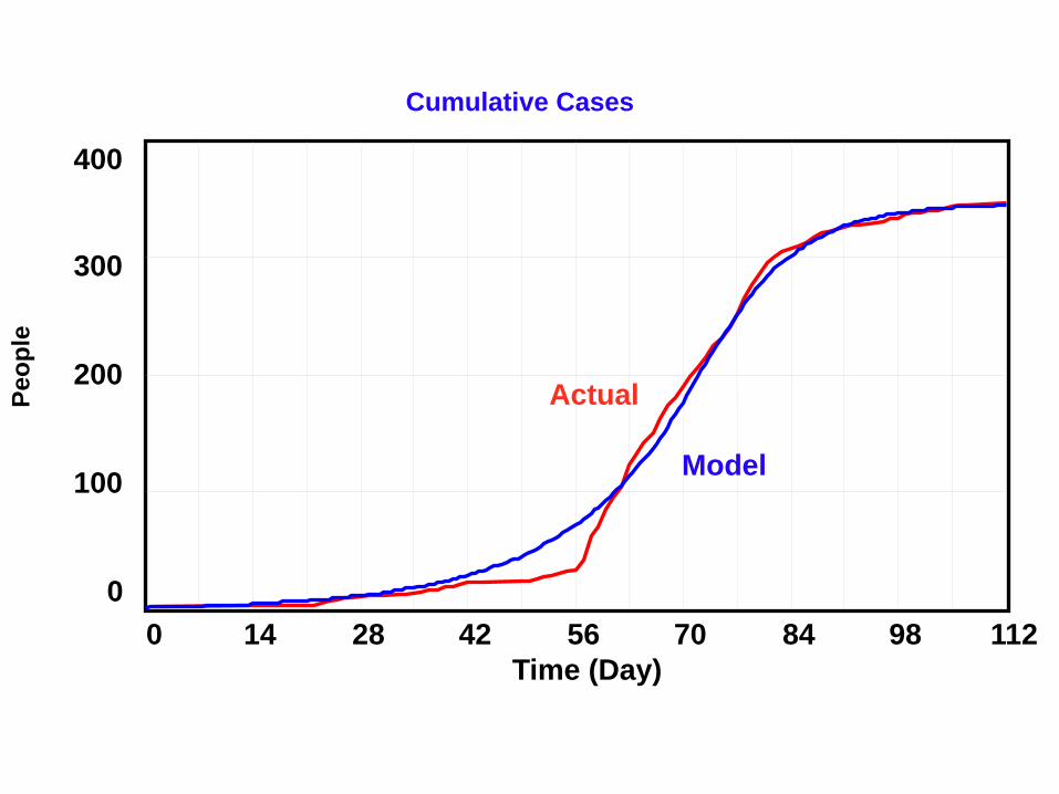
Model vs. Data with Behavioral Feedback

Cumulative Cases

400

300

200

100

0

0 14 28 42 56 70 84 98 112 Time (Day)

Peo

ple

Actual

Model

Adapted from Sterman


A Key Deliverable!



Key variables



State charts





Specification of

• Parameters











Cross-validation





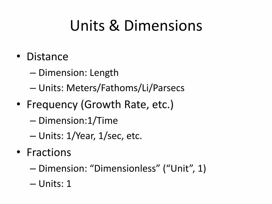
Units & Dimensions

• Distance

– Dimension: Length

– Units: Meters/Fathoms/Li/Parsecs

• Frequency (Growth Rate, etc.)

– Dimension:1/Time

– Units: 1/Year, 1/sec, etc.

• Fractions

– Dimension: “Dimensionless” (“Unit”, 1)

– Units: 1

Dimensional Analysis

• DA exploits structure of dimensional quantities to facilitate insight into the external world

• Uses – Cross-checking dimensional homogeneity of model

– Deducing form of conjectured relationship

(including showing independence of particular factors)

– Sanity check on validation of closed-form model analysis

– Checks on simulation results

– Derivation of scaling laws

* Construction of scale models

– Reducing dimensionality of model calibration, parameter estimation

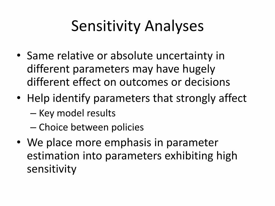
Sensitivity Analyses

• Same relative or absolute uncertainty in different parameters may have hugely different effect on outcomes or decisions

• Help identify parameters that strongly affect – Key model results

– Choice between policies

• We place more emphasis in parameter estimation into parameters exhibiting high sensitivity

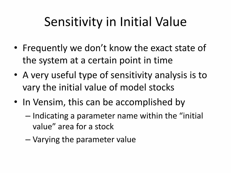
Sensitivity in Initial Value

• Frequently we don’t know the exact state of the system at a certain point in time

• A very useful type of sensitivity analysis is to vary the initial value of model stocks

• In Vensim, this can be accomplished by

– Indicating a parameter name within the “initial value” area for a stock

– Varying the parameter value

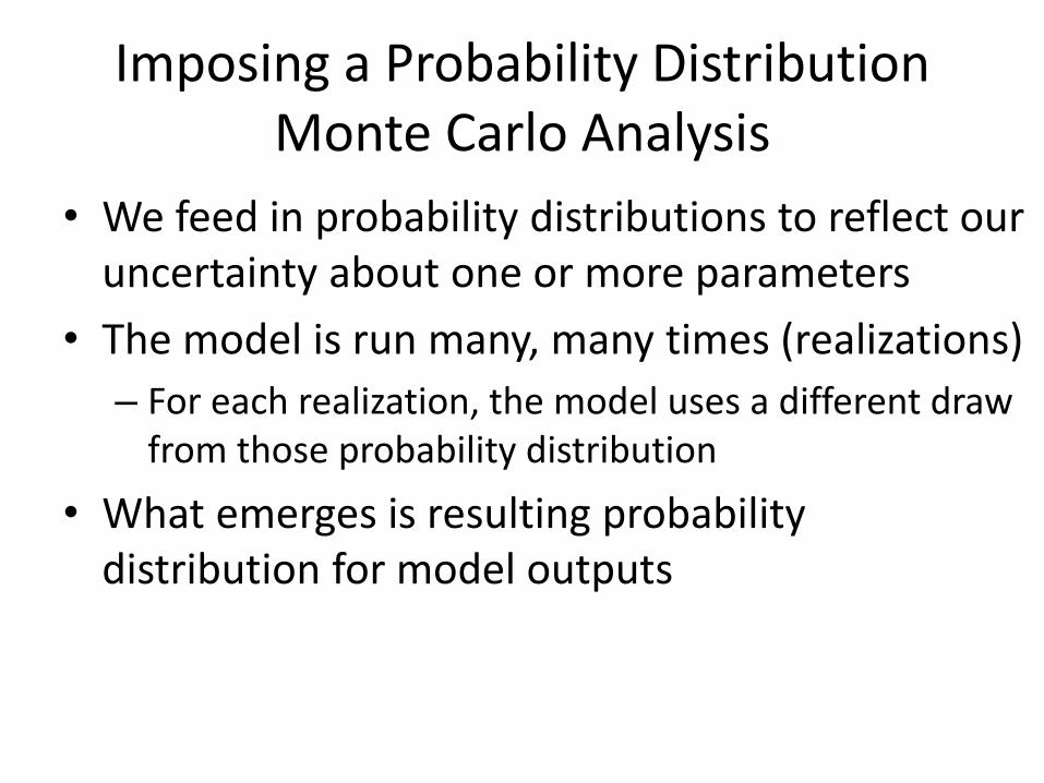
Imposing a Probability Distribution Monte Carlo Analysis

• We feed in probability distributions to reflect our uncertainty about one or more parameters

• The model is run many, many times (realizations)

– For each realization, the model uses a different draw from those probability distribution

• What emerges is resulting probability distribution for model outputs

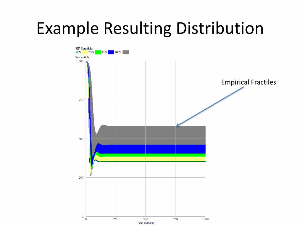
Example Resulting Distribution

Empirical Fractiles

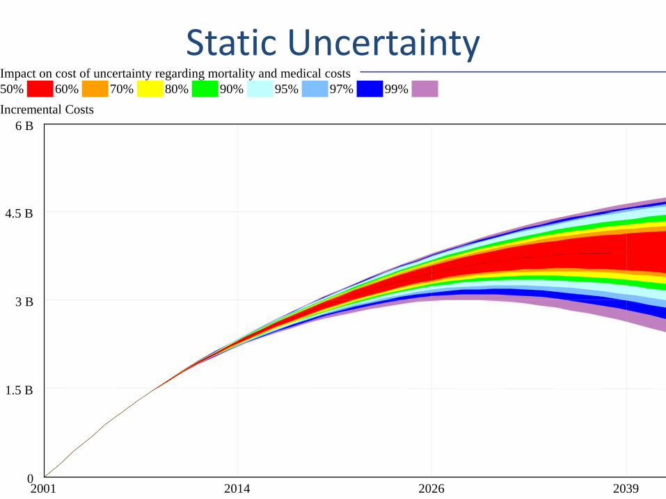
Impact on cost of uncertainty regarding mortality and medical costs

50% 60% 70% 80% 90% 95% 97% 99%

Incremental Costs

6 B

4.5 B

3 B

1.5 B

0 2001 2014 2026 2039 2051

Time (Year)

Static Uncertainty

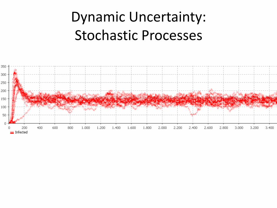
Dynamic Uncertainty: Stochastic Processes

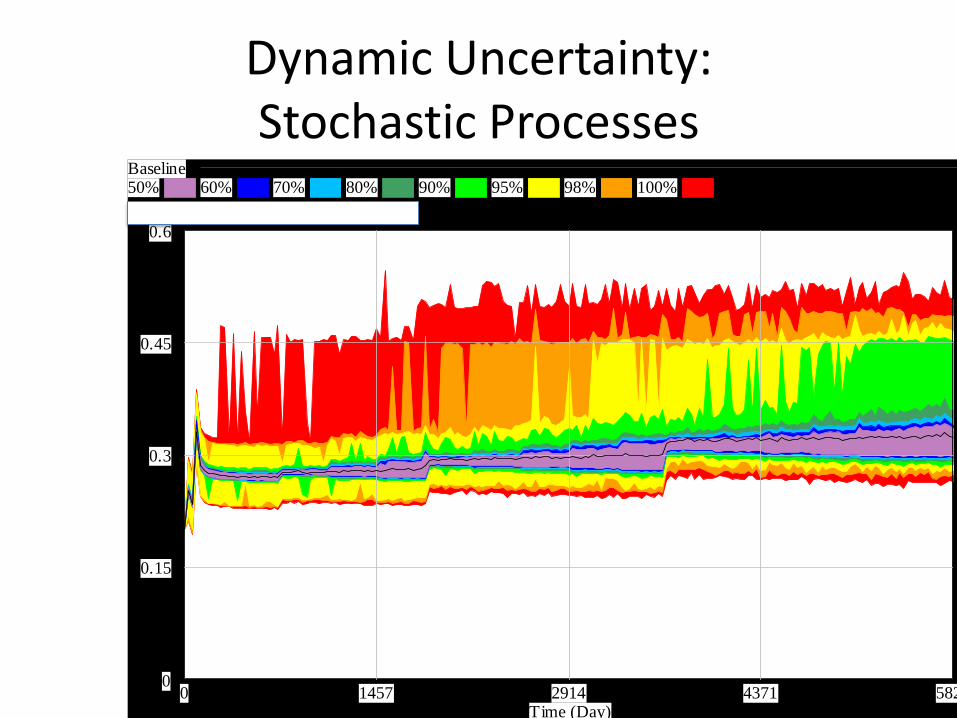
Dynamic Uncertainty: Stochastic Processes

Baseline50% 60% 70% 80% 90% 95% 98% 100%

Average Variable Cost per Cubic Meter

0.6

0.45

0.3

0.15

00 1457 2914 4371 5828

Time (Day)

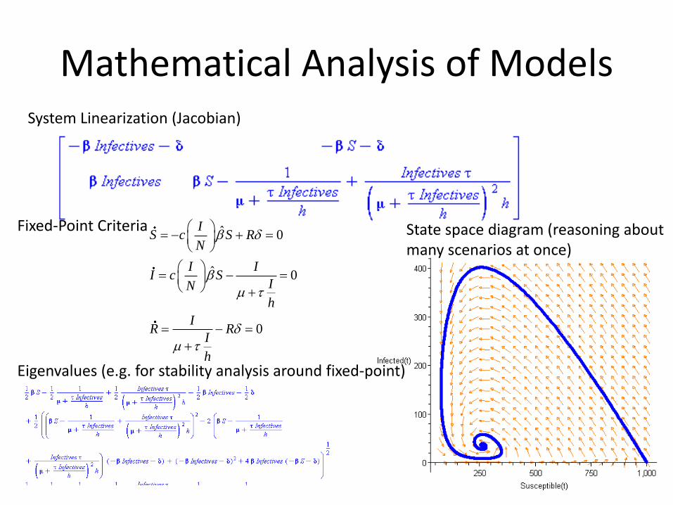
Mathematical Analysis of Models

System Linearization (Jacobian)

Fixed-Point Criteria

Eigenvalues (e.g. for stability analysis around fixed-point)

ˆ 0

ˆ 0

0

IS c S R

N

I II c S

IN

h

IR R

I

h

State space diagram (reasoning about many scenarios at once)

Applied Math & Dynamic Modeling

• Although you may not use it, the dynamic modeling presented rests on the tremendous deep & rich foundation of applied mathematics

– Linear algebra

– Calculus (Differentia/Integral, Uni& Multivariate)

– Differential equations

– Numerical analysis (including numerical integration, parameter estimation)

– Control theory

• For the mathematically inclined, the tools of these areas of applied math are available

Comments on Mathematics & Dynamic Modeling

• Many accomplished & well-published dynamic modelers have limited mathematical background

– Can investigate pressing & important issues

– Software tools are making this easier over time

• Can gain extra insight/flexibility if willing to push to learn some of the associated mathematics

• Achieving highest skill levels in dynamic modeling do require mathematical facility and sophistication

– To do sophisticated work, often those lacking this background or inclination collaborate with someone with background

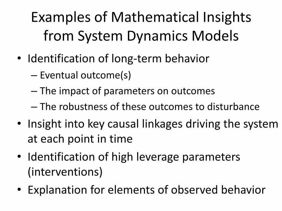
Examples of Mathematical Insights from System Dynamics Models

• Identification of long-term behavior

– Eventual outcome(s)

– The impact of parameters on outcomes

– The robustness of these outcomes to disturbance

• Insight into key causal linkages driving the system at each point in time

• Identification of high leverage parameters (interventions)

• Explanation for elements of observed behavior

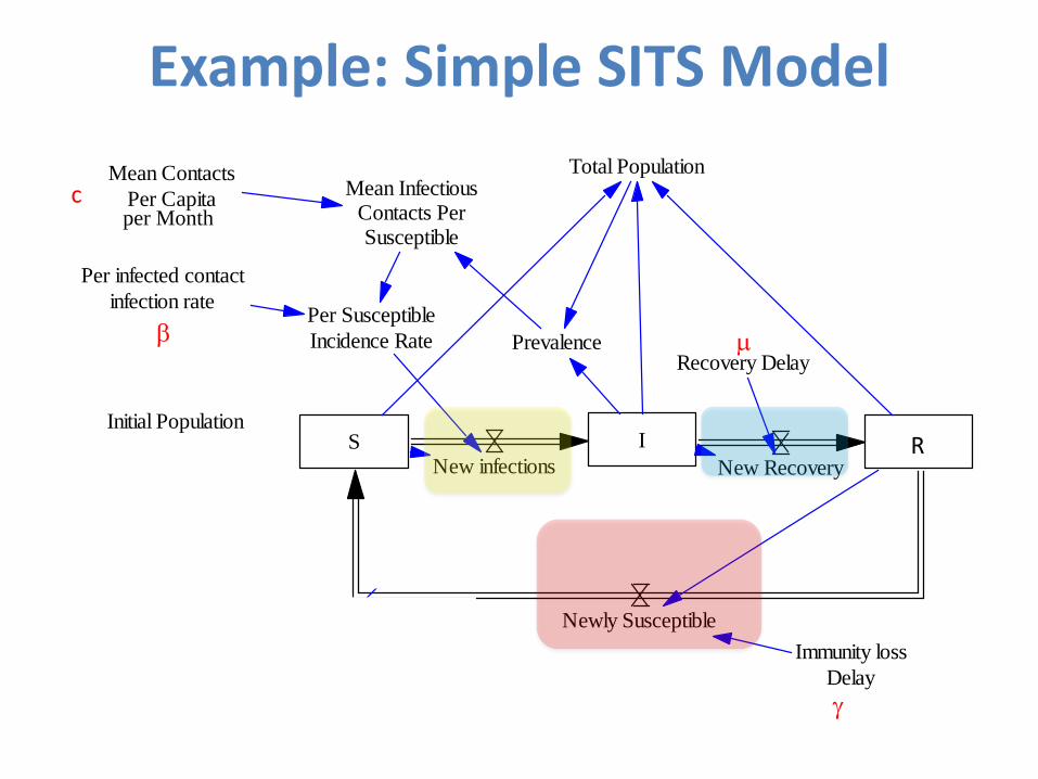
Example: Simple SITS Model

S I TNew infections New Recovery

Newly Susceptible

Immunity loss

Delay

Per infected contact

infection rate

Mean Contacts

Per Capita

Total PopulationMean Infectious

Contacts PerSusceptible

Per Susceptible

Incidence Rate

Cumulative

IllnessesNew Illness

PrevalenceRecovery Delay

Initial Population

R

c

per Month

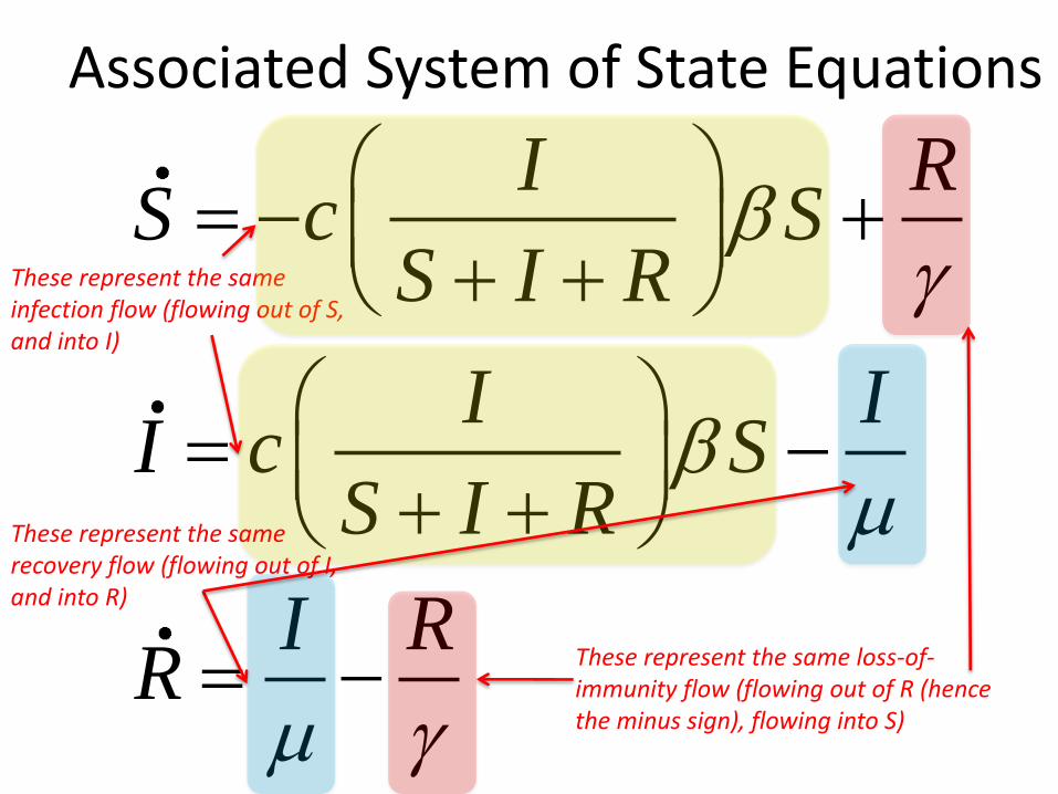
Associated System of State Equations

I R

S c SS I R

I II c S

S I R

I RR

These represent the same loss-of-immunity flow (flowing out of R (hence the minus sign), flowing into S)

These represent the same infection flow (flowing out of S, and into I)

These represent the same recovery flow (flowing out of I, and into R)


A Key Deliverable!



Key variables



State charts




Specification of

• Parameters











Cross-validation





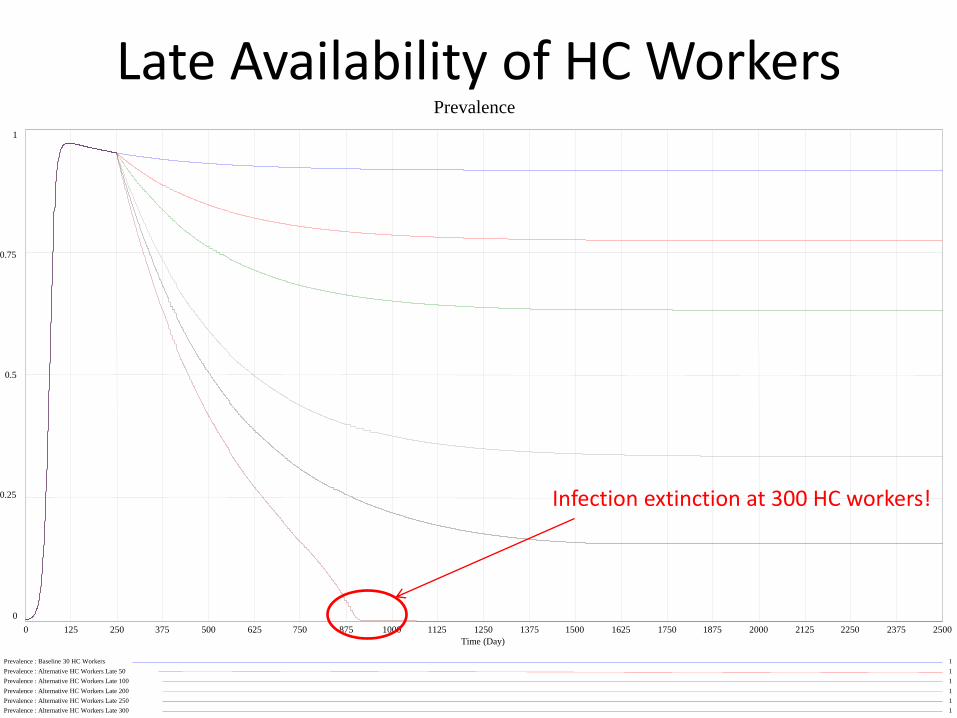
Late Availability of HC Workers

Prevalence

1

0.75

0.5

0.25

0

0 125 250 375 500 625 750 875 1000 1125 1250 1375 1500 1625 1750 1875 2000 2125 2250 2375 2500

Time (Day)

Prevalence : Baseline 30 HC Workers 1

Prevalence : Alternative HC Workers Late 50 1





Infection extinction at 300 HC workers!

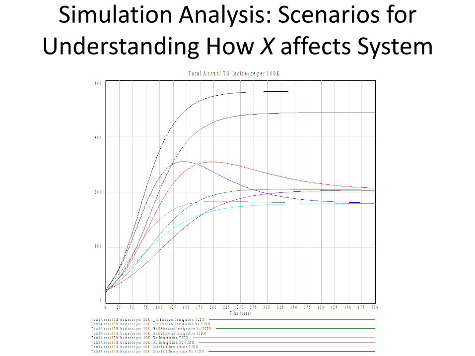
Simulation Analysis: Scenarios for Understanding How X affects System

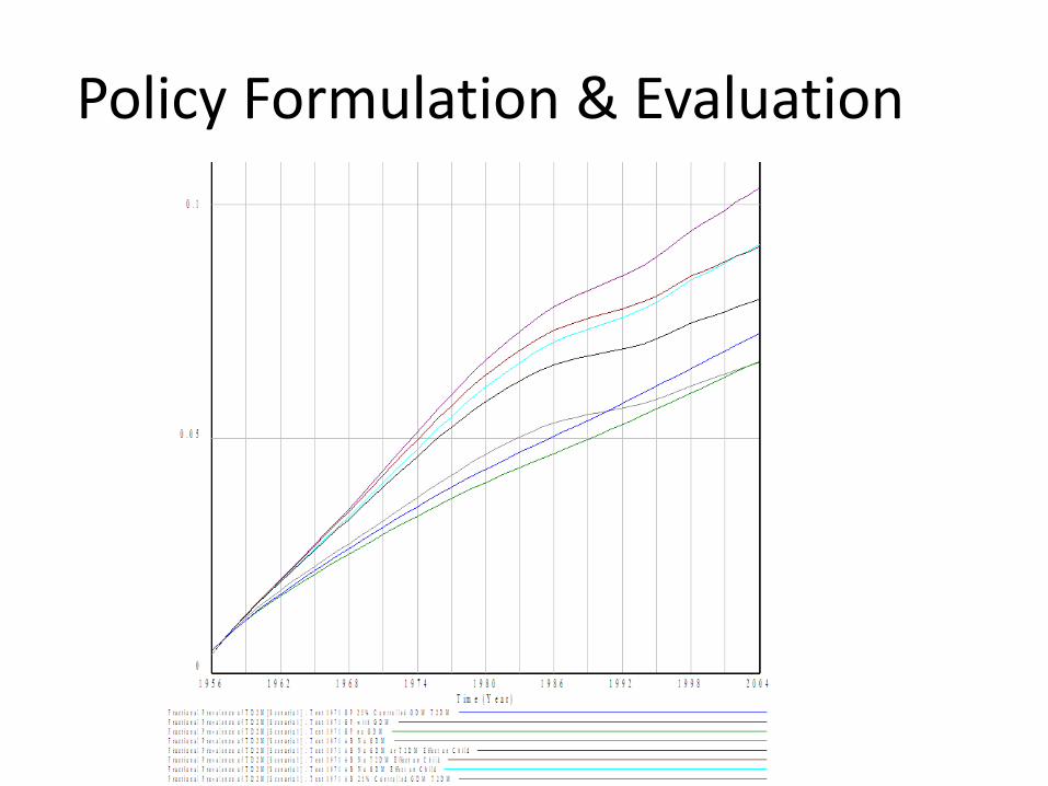
Policy Formulation & Evaluation

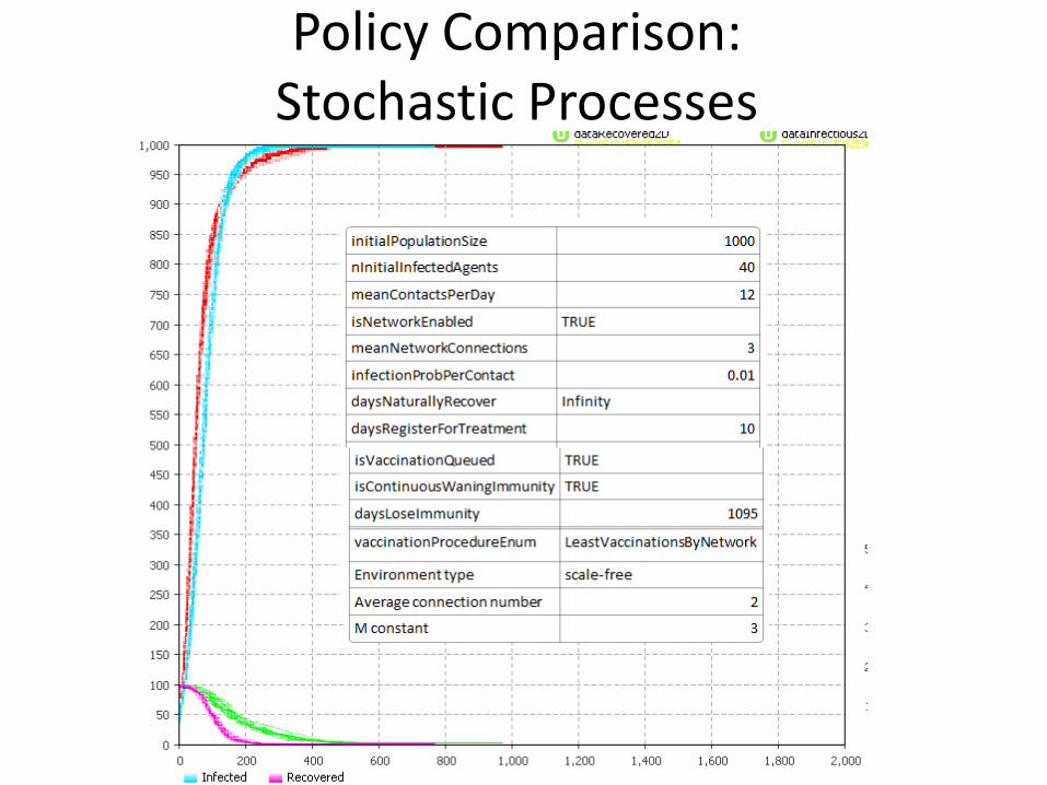
Policy Comparison: Stochastic Processes


A Key Deliverable!



Key variables



State charts




Specification of

• Parameters











Cross-validation





OVERVIEW OF THE MODEL

Total Body

Water (TBW)

extracellular fluid

volume (ECFV)+

urine flow (UFlow)

na out in urine

Extracellular

Sodium

(ECNa)

extracellular

osmolality

-

-

Antidiuretic

Hormone

(ADH)

+

AtrialNatriureticHormone(ANH)

1-

-

+

urinary

concentration

drinking

+

2-

+

+

3-

-

-

+

mean arterial

pressure (MAP)

aldosterone

(ALD)+

5-

-

-

4-

-

+

-

+

++

+

+

Simplified causal loop diagram of the overall model

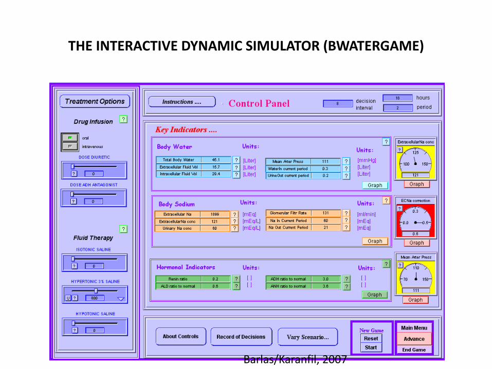
THE INTERACTIVE DYNAMIC SIMULATOR (BWATERGAME)

Barlas/Karanfil, 2007

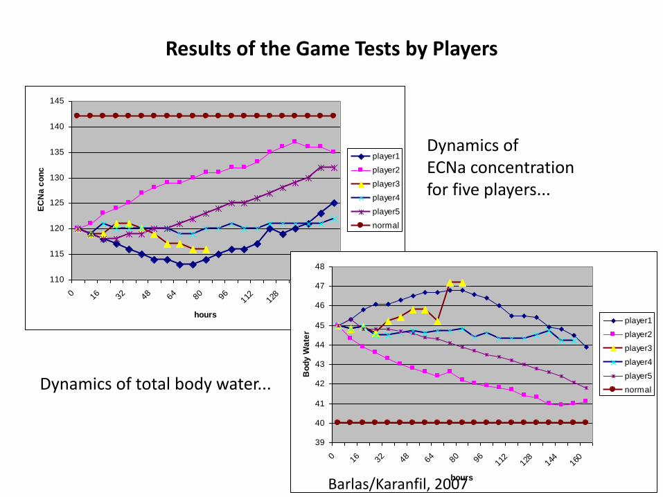
Results of the Game Tests by Players

110

115

120

125

130

135

140

145

0 16 32 48 64 80 96 112

128

144

160

hours

EC

Na

co

nc

player1

player2

player3

player4

player5

normal

Dynamics of ECNa concentration for five players...

39

40

41

42

43

44

45

46

47

48

0 16 32 48 64 80 96 112

128

144

160

hours

Bo

dy

Wa

ter

player1

player2

player3

player4

player5

normalDynamics of total body water...

Barlas/Karanfil, 2007

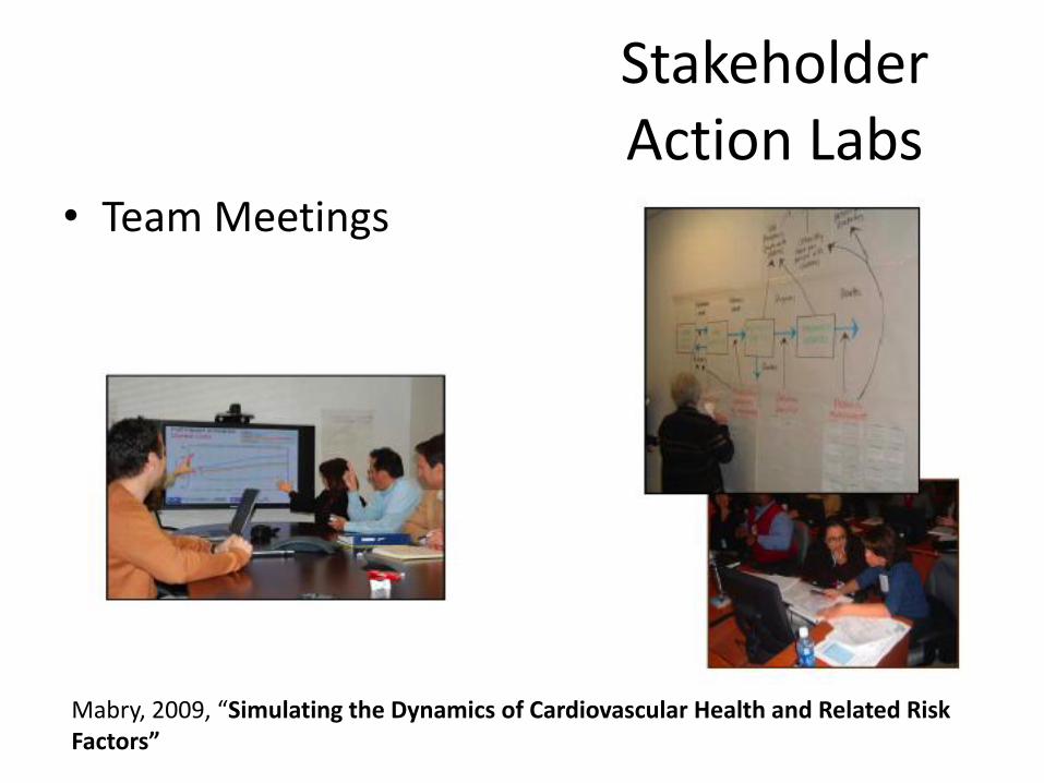
Stakeholder Action Labs

• Team Meetings

Mabry, 2009, “Simulating the Dynamics of Cardiovascular Health and Related Risk Factors”

Key Take-Home Messages from this Morning • Models express dynamic hypotheses about

processes underlying observed behavior

• Models help understanding how diverse pieces of system work together

• SD focus on feedbacks as the fundamental shapers of dynamics

• Models are specific to purpose

• System dynamics includes both qualitative & quantitative components

• SD models admit to formal reasoning & analysis


Overview of the Simulation Modeling Process of the Simulation Modeling Process Nathaniel Osgood ......

Documents

Transcript of Overview of the Simulation Modeling Process of the Simulation Modeling Process Nathaniel Osgood ......