HOW TO ANALYZE SYNCHROTRON DATA

1

SYNCHROTRON APPLICATIONS

- WHAT

Diffraction data are collected on diffractometer lines at the world’s

synchrotron sources. Most synchrotrons have one or more user

facilities or ports that perform powder diffraction experiments.

The extreme X-ray photon flux rate of a synchrotron allows users

much latitude to vary instrumental conditions. Diffractometer lines

often use custom optics and detectors designed to improve

resolution, sensitivity or capture data quickly.

2

SYNCHROTRON APPLICATIONS

- WHY

Materials can be studied dynamically while under stress,

strain, heating or cooling. The high flux rate allows users to rapidly collect many data scans as a function of conditions.

High resolution combined with high signal to noise provides improved accuracy in structure solution, phase identification and quantitative analysis.

3

SYNCHROTRON APPLICATIONS

- HOW

To best use the PDF databases for synchrotron applications, users need

to adjust applicable parameters in the database. This includes:

1) Using integrated intensity options for all entries.

2) Changing the input wavelength for all data simulations.

3) Adjusting both the optical geometry and peak width for simulations.

4) Using calculated patterns where possible. Calculated patterns have intensities

calculated from 1-1000, experimental patterns have intensities from 1-100.

5) Adjusting background and peak finding algorithms in SIeve for higher

sensitivity.

(Note: The enhanced signal to noise in most synchrotron experiments means

that low intensity peaks are often observed.)

4

Synchrotron Help

In PDF-4+ Release 2012 versions and

later, a new button was added to the

preferences setting, “Set

Synchrotron Defaults”. This changes

the wavelength, instrumental peak

profiles, and step width for all

database calculations and simulations.

The profiles were determined from

instrumental standards used at the

Argonne National Light Source. A

default wavelength of 0.7093 Å, was

used, but the user can put in any input

wavelength. Typical polarization and

specimen thicknesses were also input.

Preferences

5

COMPARISON OF EXPERIMENTAL (PD3) AND

SIMULATED DATA FOR LAB6 (USING 0.4011Å AND SYNCHROTRON DEFAULTS )

Large

Range in

Observed

Intensity

6

SYNCHROTRON DATA

VERSUS LABORATORY DATA

• Wavelengths are variable.

• Incident beam is often monochromatic and/or parallel.

• Peak resolution is high for crystalline materials (i.e.,

very small instrumental contributions to the peak

profiles, 0.01 FWHM or less).

• High count rates and signal to noise ratio are expected

for synchrotron data.

7

SYNCHROTRON DATA

Clearly resolved low intensity peaks and high signal to noise.

Peaks below

0.3% relative

intensity

8

CHANGING DISPLAY OPTIONS

USING SIEVE+

In previous slides, it was shown that display options in PDF-4+ can

be customized using preferences, which is this icon shown

in many of the display screens in PDF-4+.

9

CUSTOM DISPLAYS –

IMPORTING DATA

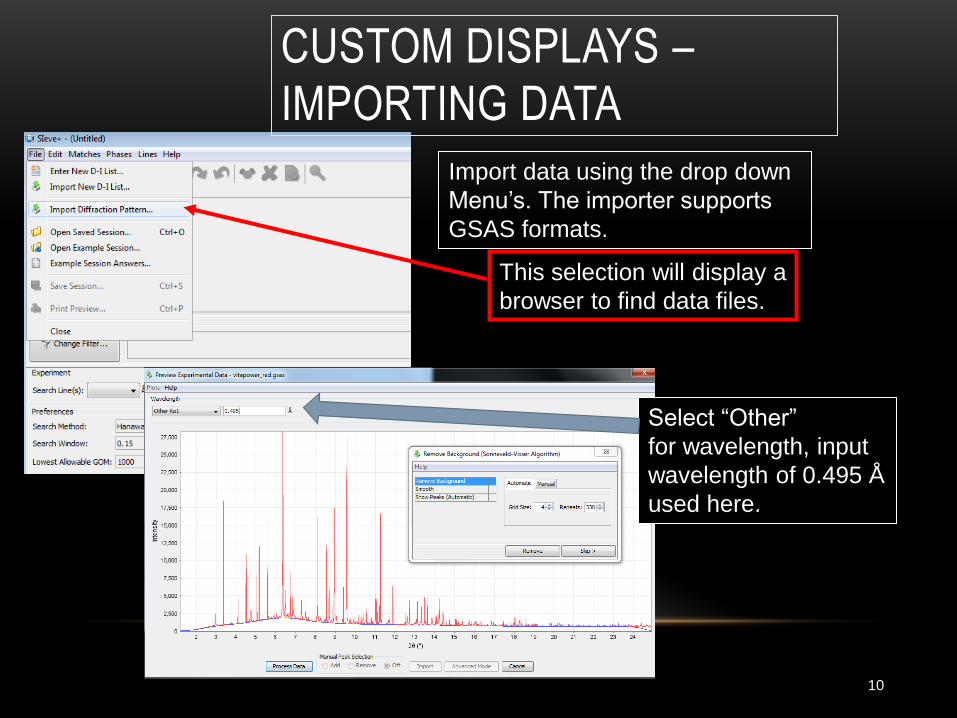
Import data using the drop down

Menu’s. The importer supports

GSAS formats.

This selection will display a

browser to find data files.

Select “Other”

for wavelength, input

wavelength of 0.495 Å

used here.

10

DATA PROCESSING After the user inputs the experimental

wavelength, a dialog box appears that

guides the user through a series of data

processing steps.

The first step is the removal of

background using a Sonneveld-Visser

algorithm. The background is highlighted

by the blue line.

This experiment used a glass capillary as

a specimen holder and the background

shown arises from incoherent scattering

from the capillary glass.

Depending on the specimen size and

capillary wall thickness in relation to the

beam size, sometimes the capillary

scatter will be easily observed and other

times will not.

11

Peak Finding Peak finding uses a second

derivative algorithm. Due to the

exceptionally good signal to noise

ratio in synchrotron data, it is

usually best to set the derivative

and intensity detection limits to very

low numbers. It is also helpful to

use the mouse to drag and magnify

the plot so that minor peaks can be

identified.

In this multiphase specimen, 355

peaks were found and some

were still not identified and had to

be chosen by manual methods.

This is a point and click option at

the bottom of the page.

Manual selection option 12

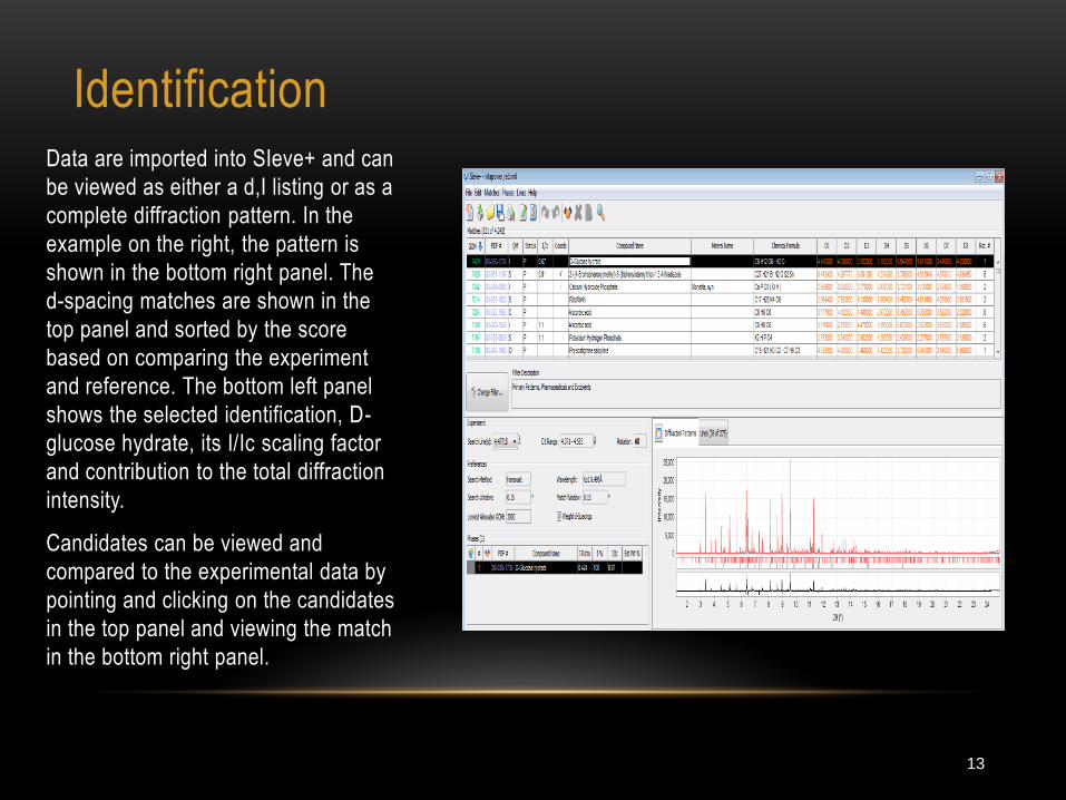
Identification Data are imported into SIeve+ and can

be viewed as either a d,I listing or as a

complete diffraction pattern. In the

example on the right, the pattern is

shown in the bottom right panel. The

d-spacing matches are shown in the

top panel and sorted by the score

based on comparing the experiment

and reference. The bottom left panel

shows the selected identification, D-

glucose hydrate, its I/Ic scaling factor

and contribution to the total diffraction

intensity.

Candidates can be viewed and

compared to the experimental data by

pointing and clicking on the candidates

in the top panel and viewing the match

in the bottom right panel.

13

Multi-phase

Identification At any time, the user can choose to view a multiphase comparison by using a right click of the mouse on the previously shown (slide 13) screen in SIeve+.

Selection of “Open Simulated Profile with Experimental Data” will produce a comparison of selected phases with the candidate phases in a single plot.

The use of “synchrotron defaults” as shown in slide 5 will produce a plot with appropriate peak profiles for synchrotron data.

In this comparison, the raw data in a vitamin pill is compared to vitamin C, glucose hydrate, iron fumarate and vitamin B.

14

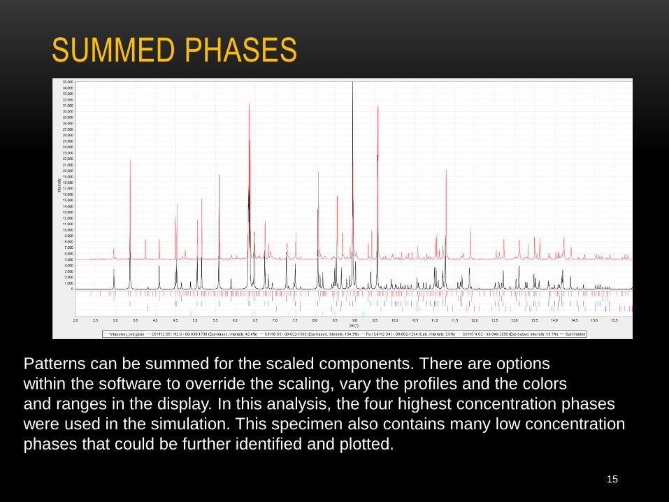
SUMMED PHASES

15

Patterns can be summed for the scaled components. There are options

within the software to override the scaling, vary the profiles and the colors

and ranges in the display. In this analysis, the four highest concentration phases

were used in the simulation. This specimen also contains many low concentration

phases that could be further identified and plotted.

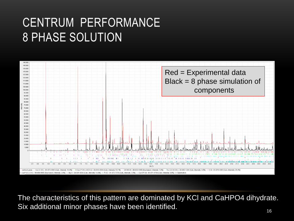
CENTRUM PERFORMANCE

8 PHASE SOLUTION

16

The characteristics of this pattern are dominated by KCl and CaHPO4 dihydrate.

Six additional minor phases have been identified.

Red = Experimental data

Black = 8 phase simulation of

components

SUMMARY

17

• New features have been added to the PDF-4+ database and associated software SIeve+

specific to synchrotron analyses.

• An option in the preferences module of PDF-4+ automatically changes several

instrument settings to those found in global synchrotron facilities.

• Instrument profile settings can be user customized, the preference module saves time and

convenience when processing synchrotron diffraction data sets.

• Dynamic memory has been reallocated within the product to allow larger data sets (typical

of synchrotron data), to be quickly processed for rapid identification.

• Q and d-spacing plotting options have been added to Release 2013 Products.

MORE INFORMATION

For more information on how to perform complex multi-phase simulations, see the

pattern simulations tutorial.

For more information on how to identify minor phases (below 10 wt %),

see the tutorial and publication on “Data Mining – Trace Phase Analysis”.

For more information on synchrotron instrument functions as used in simulations

and Rietveld refinements see the following:

J. A. Kaduk and J. Reid, (2011), “Typical values of Rietveld instrument

profile Coefficients”

Powder Diffraction / Volume 26 / Issue 01 / March 2011, pp 88-93

Copyright © Cambridge University Press 2011

DOI: http://dx.doi.org/10.1154/1.3548128

Published online: 05 March 2012

Note: Several authors have now reported identification of phases in concentrations

below 0.3 wt % using synchrotron data. Significantly lower detection limits are

possible with optimized (signal/noise) experiments.

18