The object-oriented terminology and formats for class diagrams used in this document are based on Booch's notation (Booch1994). The following terms are used in this chapter:

Object-Oriented Programming (OOP): a programming method in which programs are organized as cooperative collectionsof objects that represent an instance of some class, and whose classes are all members of a hierarchy of classes unitedvia inheritance relationships.

Class: a set of objects that share a common structure and a common behavior.Object: an instance of a class.Instantiation: a new object created from a class.Hierarchy: a ranking or ordering of abstractions.Inheritance: a mechanism of hierarchy in which one class shares the structure or behavior defined in one or more classes;

there is single or multiple inheritance.Aggregation: a mechanism of hierarchy wherein a class mimics the behavior of one or more classes by embedding their

instances. Polymorphism: the property of an object, achieved through either inheritance or aggregation, through which it represents

objects of many different classes.Persistence: the property of an object through which its existence transcends time and/or space; the object becomes capable

of existing past the lifetime and address space of its creator (e.g., hard disk).Runtime Type Identification: the property of an object through which it stores the identity of its class so that it is capable of

identifying its class type when queried.

6-1

Chapter 6Symbolic Modeling of River Basin Systems

This chapter documents the basic architecture of the Aquarius software and discusses the advantagesof using an object-oriented programming framework for modeling the hydraulic and mathematicalconnectivity of the flow network components. Comprehension of the material in this section is notessential for using Aquarius, and is helped by reading Chapter 7.

Object-Oriented Programming Framework

Earlier computer models for solving water resource problems have used algorithmic computerlanguages such as FORTRAN. Although these languages are well suited for numerical or algorithm-oriented models, they lack the flexibility to allow for alterations, additions, or deletions of flownetwork components. Recent research has overcome this problem by using an object-orientedprogramming (OOP) language1, specifically C++. Objects are the building blocks of an OOP. Anobject contains properties that communicate with other objects. In turn, object behavior is controlledby methods, which are the rules and algorithms that tell an object how to act on the data it receivesin its input slots. Objects may inherit both data (properties) and behavior (methods) from otherhigher-level objects.

Water systems are ideal candidates for modeling through an object-oriented framework. A watersystem may include different types of water components, including reservoirs, powerplants,diversions or junction points, irrigation areas, environmentally-sensitive river reaches, etc, whichcan be interpreted as objects of a flow network in which they interact. Aquarius models eachcomponent or structure of the water system as an equivalent node or object in the programming

6-2

Figure 6.1 Aquarius top-level class diagram.

environment. In modeling terms, a physical link (e.g., a river reach) connecting two systemcomponents becomes an outflow slot of the upstream object connected to an inflow slot of thedownstream object.

The user interacts with the model through a graphical user interface (GUI) that allows the analystto readily create the river basin network of interest. This is a simple task due to the inherentcapability of the object oriented paradigm for graphical representation. During the creation of theflow network, each system component (object) corresponds to a graphical network node. Thesenodes are represented by icons, which are a pictorial representation of the object. By dragging oneof these icons from the menu, the model creates an instance of the object on the screen. Thisprocedure also allows the user to connect graphically the input slots of this object with the outputslots of one or more objects. By clicking on the icon, the object displays data slots for input andoutput and also allows the user to visually inspect for incorrect or missing data. Details on the useof the GUI are in Chapter 7.

Software Architecture

The overall design of Aquarius is depicted by the top-level class diagram in figure 6.1. As indicatedin the figure, all classes implemented in Aquarius are organized into three basic class categories:

C Network Worksheet (NWS)C Water System Components (WSC)C Water System Links (WSL)

6-3

Aquarius is built upon Microsoft Foundation Classes (MFC), which are a set of reusable classes thatprovide, with minimal overhead, numerous important functions to software applications written forMicrosoft Windows.

Network Worksheet

The Network Worksheet (NWS), one of the basic classes of Aquarius, is composed of two classes–document and view– that are responsible for storing and rendering to the screen, respectively, dataassociated with any flow network. The document is a data object that the user interacts with duringediting sessions; for instance, during the creation or alteration of a flow network. View is the user'swindow to the data, which specifies how the user sees the document's data and interacts with it.Data pertaining to the network, which is also an object, are stored in the document, and the objectsthemselves are rendered onto the view window. Most of the important functions of the software,such as user interaction, data persistence, and optimization algorithms, are routed to the individualobjects via the message handling facility of the view window.

The document portion of the NWS stores the other two basic class categories of Aquarius, the WaterSystem Components (WSC) and the Water System Links (WSL).

Water System Components

The Water System Components (WSCs) are defined by several classes, depending on the componentof the flow network that requires representation, although all WSCs are derived from a single basicclass, CNode. In addition to the data corresponding to the individual network components, thedocument class also stores global data corresponding to the whole network (for instance, parameterscontrolling the optimization algorithm, the selected period of analysis, output data related to theoptimal solution, etc.).

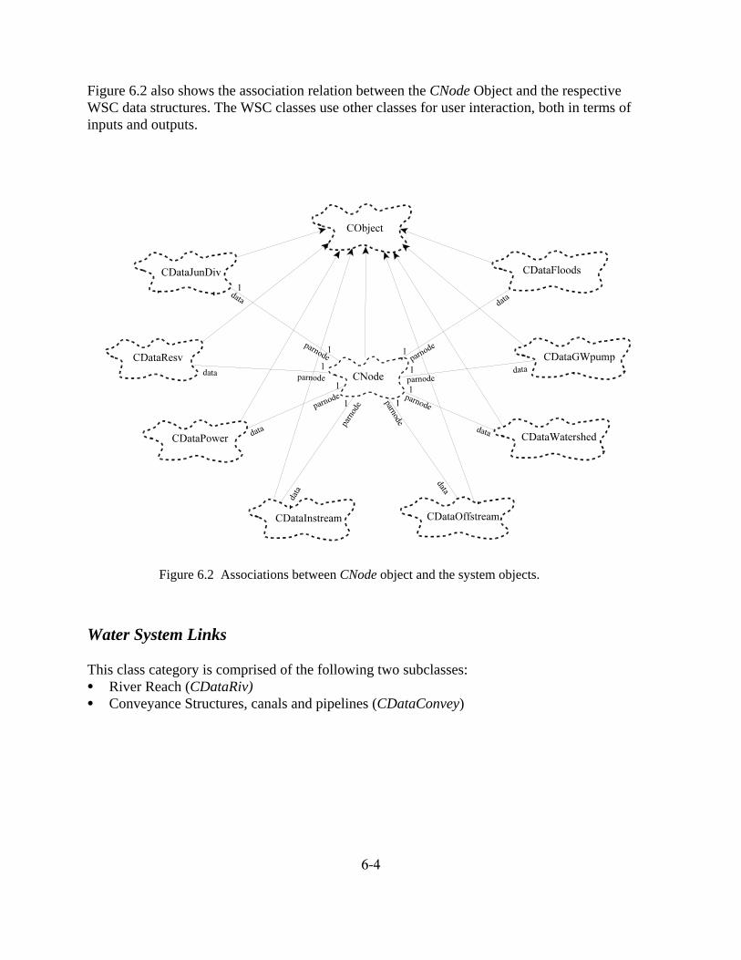
As illustrated in figure 6.2, the data structure object can be an instance of any of the following classes:

C CDataJunDiv (junctions and diversions)C CDataResv (storage capacities)C CDataPower (hydroelectric plants)C CDataOffstream (offstream demand areas)C CDataInstream (instream demand areas) C CDataWatershed (Surface water sources)C CDataGWpumping (Groundwater pumping)C CDataFloods (flood control reaches)

6-4

Figure 6.2 Associations between CNode object and the system objects.

Figure 6.2 also shows the association relation between the CNode Object and the respectiveWSC data structures. The WSC classes use other classes for user interaction, both in terms ofinputs and outputs.

Water System Links

This class category is comprised of the following two subclasses:C River Reach (CDataRiv) C Conveyance Structures, canals and pipelines (CDataConvey)

6-5

During “validation” of the network (discussed in Chapter 7) WSLs are classified according to therole they play and the place they occupy in the flow network. The classification of links is performedautomatically by the model, which names the links according to the following definitions:

natflow arc conveying surface water from a basin (SWS).

decision arc conveying water released from a reservoir, diversion node or pumping well under thefollowing types:(i) a controlled release from a reservoir serving an offstream water user (HPW, IRR or M&I),directly connected to the reservoir of reference;(ii) a controlled release from a reservoir serving an instream water user (IRA or FCA), directlyconnected to the reservoir of reference;(iii) a controlled release from a reservoir directly to an RDD object, which in turn servesdemand area/s located farther downstream (and mathematically disconnected) from the reservoirof reference;(iv) a controlled release from a reservoir directly into a downstream reservoir (no water userin between);(v) a controlled water diversion through the offstream link of a diversion node; (vi) a controlled withdrawn (pumping) of water from an aquifer (GWS);

return arc carrying return flows from an offstream demand area (IRR and M&I) back to a river reachor reservoir.

spill arc evacuating spillages from a reservoir (always the central link).

dec&spill arc acting as a decision and as a spill arc at the same time (dual classification).

Mathematical Connectivity of System Components

Solving the water allocation problem in Chapter 5 for any user-defined network requires anautomated procedure to handle the formulation mathematics. In Aquarius the mathematicalconnectivity of the system components is derived automatically from the linkage of the objectscomprising the network, which in turn reflects the direction of flow from one structure to the next(i.e., their hydraulic connectivity).

The requirements for the mathematical connectivity of the system components may vary dependingon the characteristics of the optimization technique being implemented. For the optimizationtechnique used in this model (Sequential Quadratic Programing) the mathematical connectivity ofa river network serves to:

C Assemble the gradient vector and Hessian matrix of the second order approximation of the totalobjective function (see Chapter 5, Solution Method).

C Build up the set of operational constraints (see Chapter 5, Operational Restrictions).

6-6

Figure 6.3 Network that demonstrates mathematical connectivity.

The tasks indicated above required the development of an algorithm capable of automaticallygathering information from the network about controlled and uncontrolled flows occurring upstreamand downstream from a given system component. The way water sources, storage reservoirs, anddemand zones are arranged in a river basin (i.e., network topology) determines the hydraulic andmathematical dependence among them. Controlled and uncontrolled flows occurring upstream froma given node influence the decisions at that node.

Figure 6.3 represents a river system that illustrates the intricacies of mathematical connectivity. Thesystem has two headwater reservoirs (B and C) with hydropower facilities (the powerplantconnected to reservoir C is a run-of-the-river type). Releases from the powerplants linked to theheadwater reservoirs plus additional releases from Reservoir C to supplement downstream demandsbecome regulated inflows to downstream reservoir A, which in turns supplies water to mostdownstream demand areas including hydropower, urban supply and a fish habitat protection area.An irrigation demand zone and an instream recreation area are in the middle of the system.

The series of physical links (river reaches, canals/pipelines) connecting surface water sources,storage capacities, and demand areas are used by the model to automatically formulate themathematical structure of the water allocation problem. First, the model identifies the decision setsthat control water allocation in the flow network. Six decision sets: dA , dB , dC , dD , dE , dF areidentified and randomly numbered by the model. Links conveying controlled flows are distinguishedby dashed lines in figure 6.3. According to the classification given above (Water System Links)decision sets dA , dB, dC , dE are type (i), decision set dF is type (iii) and the set dD is type (iv).

The model then collects information regarding all controlled and uncontrolled flows in the networkusing a recursive search algorithm. Some of the output generated by the search procedure is in table

6-7

Table 6.1 Table of mathematical connectivity. dA dB dC dD dE dF WSC -1.00 -1.00 1.00 -0.70 1.00 1.00 Reservoir A

0.00 0.00 0.00 0.00 -1.00 0.00 Reservoir B0.00 0.00 -1.00 0.00 0.00 -1.00 Reservoir C1.00 0.00 0.00 0.00 0.00 0.00 Hydroplant A0.00 0.00 0.00 0.00 1.00 0.00 Hydroplant B0.00 0.00 1.00 0.00 0.00 0.00 Hydroplant C0.00 0.00 1.00 -1.00

0.00 Fish Habitat 0.00 0.00 0.00 0.00 0.00 1.00 RDD

6.1, which shows the coefficients of the six decision sets. For example, the first row corresponds toreservoir A, where the 1.00 values for decision sets dC and dE correspond to controlled releases fromthe two upstream powerplants. The 1.00 value for decision set dF corresponds to additionalcontrolled releases from reservoir C (central outlet work) to help satisfy the downstream demands.All three releases enter reservoir A as controlled inflows. Decision set dD carries a coefficient equalto -0.7. The value and sign assigned to this coefficient indicates that 70 percent of the water divertedfrom the river into the irrigation area is consumptively used, with the remaining 30 percent (r = 0.3for the irrigation area) reaching reservoir A via return flows. The remaining two coefficients, -1.00values for decision sets dA and dB , represent controlled releases from the reservoir underconsideration. The values in table 6.1 can be accessed in the model using the available softwaremenus (see Chapter 7, Exploring the Network Worksheet Screen).

Figure 6.4 shows the coefficients listed in table 6.1 plus some additional information, alsogathered by the search procedure, for all nodes composing the example network in figure 6.3.This information, which is stored as part of the objects data structure, is used by the model toautomatically build the set of constraint equations and compute the gradient vector and Hessianmatrix. The information collected is organized in four quadrants: controlled inflows XI at theupper-left corner, uncontrolled inflows UI at the lower-left corner, controlled releases XR at theupper-right corner (alternatively the return coefficient r for WSCs with consumptive use), anduncontrolled releases at the lower-right corner. The superscript for UI and UR indicates theoriginating reservoir. The reader can check the information in figure 6.4 with assistance fromfigure 6.3 and table 6.1.

6-8

Constraint Set Assemblage

The model is capable of attaching operational constraints to the following system components (seeChapter 5, Operational Restrictions, for more details): C storage reservoir (RES)C reservoir with lake recreation (RLR)C hydropower plants (HPW)C instream water demands: recreation (IRA) and flow protection (IFP)C offstream demand areas: municipal water supply (M&I) and irrigation (IRR)C flood control river reaches (FCA)C groundwater source (GWP),

After the user specifies which operational constraints are included in the formulation of the waterallocation problem, the NWS delegates the responsibility for building the set of restrictions to eachof the components listed above.

The information required by the system components for the global task of computing the right- andleft-hand-sides of the equality and inequality constraints is gathered from the network, using therecursive algorithms outlined previously. Once the NWS completes the constraint set computation,the information is passed to the optimization routine.

6-9

Figure 6.4 Information collected by the search algorithms.

6-10

Note: XR for offstream water (IRR and M&I) is replaced by the return flow coefficient r.

Figure 6.4 Information collected by the search algorithms (continued).

6-11

Gradient Vector and Hessian Matrix Assemblage

How water storages and demands are arranged in a river basin determines the physical andmathematical interdependence among them. For instance, in figure 6.3, releases from the headwaterreservoirs become regulated inflows to the downstream reservoir, which supply water to theremaining portion of the system. The series of links connecting the various components of a flownetwork defines the mathematical linkage among the sets of decision variables and consequently thestructure of the gradient vector Lf and Hessian matrix H in equations (5.4) and (5.5), respectively.Diaz and Fontane (1989) demonstrated, in an earlier more exclusive study solely on hydropower,that it is possible to identify geometrical patterns in the mathematical structure of the gradient vectorand global Hessian regarding the topology of the flow network. In this study we extended theaforementioned work to river basins with multiple water uses.

Aquarius first identifies all controlled and uncontrolled flows present in the network, thenautomatically builds the gradient vector and Hessian matrix. The assemblage of Lf and H isdetermined based on information provided by the network search procedures and the library ofpartial derivatives introduced in Appendix A. The algebraic expressions of the first and secondorder partial derivatives of the benefit functions are a property of each water user. For theexample network shown in figure 6.3, there are six basic groups of first partial derivatives(Mƒ/MdA Mƒ/MdB , Mƒ/MdC , Mƒ/MdD , Mƒ/MdE , Mƒ/MdF ), one for each decision set, which containderivatives for np time periods. The computation of the gradient vector results from thecombination of the following equations:

= Eq.(A.1) for i=1, 2, ..., np

= Eq.(A.21) + Eq.(A.2) for i=1, 2, ..., np

= Eq.(A.1) + Eq.(A.24) + Eq.(A.3) for i=1, 2, ..., np

= Eq.(A.18) + Eq.(A.24) + Eq.(A.3) for i=1, 2, ..., np

= Eq.(A.1) + Eq.(A.24) + Eq.(A.3) for i=1, 2, ..., np

Assembly of the global Hessian matrix (i.e., the Hessian for the entire network) follows rules similarto those used for assembling the gradient vector, although, because of the presence of second cross-partial derivatives, it may appear more involved. Again, the mathematical connectivity of the

6-12

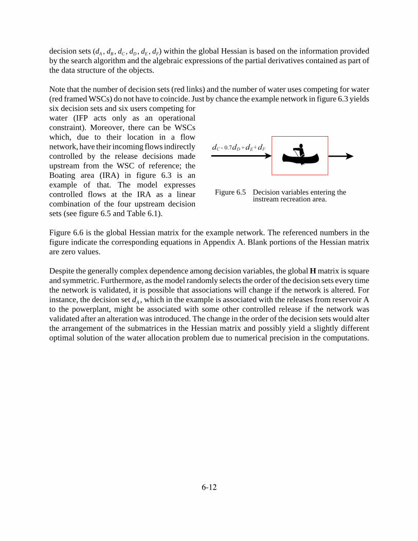
Figure 6.5 Decision variables entering the instream recreation area.

decision sets (dA , dB , dC , dD , dE , dF) within the global Hessian is based on the information providedby the search algorithm and the algebraic expressions of the partial derivatives contained as part ofthe data structure of the objects.

Note that the number of decision sets (red links) and the number of water uses competing for water(red framed WSCs) do not have to coincide. Just by chance the example network in figure 6.3 yieldssix decision sets and six users competing forwater (IFP acts only as an operationalconstraint). Moreover, there can be WSCswhich, due to their location in a flownetwork, have their incoming flows indirectlycontrolled by the release decisions madeupstream from the WSC of reference; theBoating area (IRA) in figure 6.3 is anexample of that. The model expressescontrolled flows at the IRA as a linearcombination of the four upstream decisionsets (see figure 6.5 and Table 6.1).

Figure 6.6 is the global Hessian matrix for the example network. The referenced numbers in thefigure indicate the corresponding equations in Appendix A. Blank portions of the Hessian matrixare zero values.

Despite the generally complex dependence among decision variables, the global H matrix is squareand symmetric. Furthermore, as the model randomly selects the order of the decision sets every timethe network is validated, it is possible that associations will change if the network is altered. Forinstance, the decision set dA , which in the example is associated with the releases from reservoir Ato the powerplant, might be associated with some other controlled release if the network wasvalidated after an alteration was introduced. The change in the order of the decision sets would alterthe arrangement of the submatrices in the Hessian matrix and possibly yield a slightly differentoptimal solution of the water allocation problem due to numerical precision in the computations.

6-13

Figure 6.6 Global Hessian matrix for the example network in Figure 6.3 (equations from Appendix A)