Swarm Intelligence – W5:Swarm Intelligence for

Machine Learning:An Introduction to

Genetic Algorithms andParticle Swarm Optimization

Outline

• Machine-learning-based methods– Rationale for real-time, embedded systems– Classification and terminology

• Genetic Algorithms (GA)– Terminology– Main operators and features

• Particle Swarm Optimization (PSO)– Terminology– Main operators and features

• Comparison between GA and PSO

Initialize

Perform main loop

End criterion met?

End

Start

N

Y

Rationale and Classification

Why Machine-Learning?• Complementarity to a model-based/engineering

approaches: when low-level details matter (optimization) and/or good models do not exist (design)!

• When the design/optimization space is too big (infinite)/too computationally expensive to be systematically searched

• Automatic design and optimization techniques• Role of engineer reduced to specifying

performance requirements and problem encoding

Why Machine-Learning?

• There are design and optimization techniques robust to noise, nonlinearities, discontinuities

• Individual real-time adaptation to new environmental conditions; i.e. increased individual flexibility when environmental conditions are not known/cannot predicted a priori

• Search space: parameters and/or rules

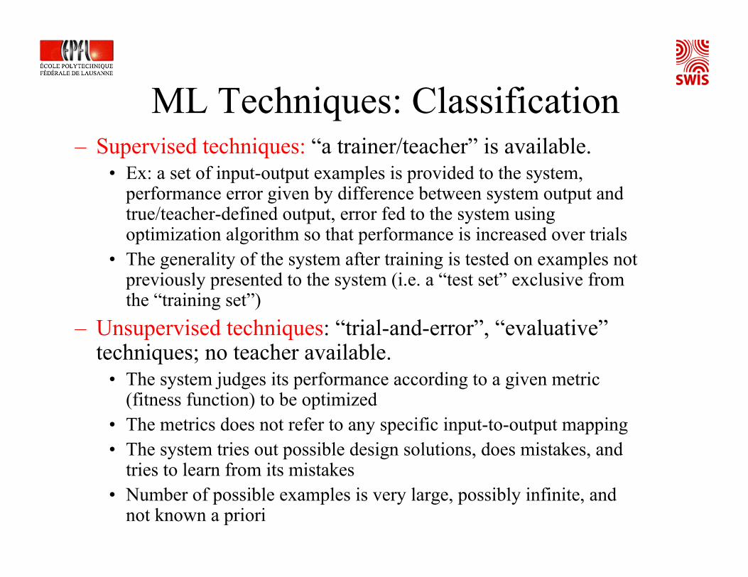
ML Techniques: Classification– Supervised techniques: “a trainer/teacher” is available.

• Ex: a set of input-output examples is provided to the system, performance error given by difference between system output and true/teacher-defined output, error fed to the system using optimization algorithm so that performance is increased over trials

• The generality of the system after training is tested on examples not previously presented to the system (i.e. a “test set” exclusive from the “training set”)

– Unsupervised techniques: “trial-and-error”, “evaluative”techniques; no teacher available.

• The system judges its performance according to a given metric (fitness function) to be optimized

• The metrics does not refer to any specific input-to-output mapping• The system tries out possible design solutions, does mistakes, and

tries to learn from its mistakes• Number of possible examples is very large, possibly infinite, and

not known a priori

ML Techniques: Classification

– Off-line: in simulation, download the learned/evolved solution onto real hardware when certain criteria are met

– Hybrid: most of the time in simulation (e.g. 90%), last period (e.g. 10%) of the process on real hardware

– On-line: from the beginning on real hardware (no simulation). Depending on the algorithm more or less rapid

ML Techniques: Classification

– On-board: machine-learning algorithm run on the system to be learned or evolved (no external unit)

– Off-board: the machine-learning algorithm runs off-board and the system to be learned or evolved just serves as phenotypical, embodied implementation of a candidate solution

ML algorithms require sometimes fairly important computational resources (in particular for multi-agent search algorithms), therefore a further classification is:

Selected Unsupervised ML Techniques Robust to Noisy

Fitness/Reinforcement Functions• Evolutionary computation

– Genetic Algorithms (GA) – Genetic Programming (GP)– Evolutionary Strategies (ES)– Particle Swarm Optimization (PSO)

• Learning – In-Line Adaptive Learning– Reinforcement Learning

Today

Week 8

Today

Genetic Algorithms

Genetic Algorithms Inspiration• In natural evolution, organisms adapt to

their environments – better able to survive over time

• Aspects of evolution:– Survival of the fittest– Genetic combination in reproduction– Mutation

• Genetic Algorithms use evolutionary techniques to achieve parameter optimization

GA: Terminology• Population: set of m candidate solutions (e.g. m = 100); each candidate

solution can also be considered as a genetic individual endowed with a single chromosome which in turn consists of multiple genes.

• Generation: new population after genetic operators have been applied (n = # generations e.g. 50, 100, 1000).

• Fitness function: measurement of the efficacy of each candidate solution

• Evaluation span: evaluation period of each candidate solution during a given generation. The time cost of the evaluation span differs greatly from scenario to scenario: it can be extremely cheap (e.g., simply computing the fitness function in a benchmark function) or involve an experimental period (e.g., evaluating the performance of a given control parameter set on a robot)

• Life span: number of generations a candidate solution survives

• Population manager: applies genetic operators to generate the candidate solutions of the new generation from the current one

• Principles: selection (survival of the fittest), recombination, and mutation

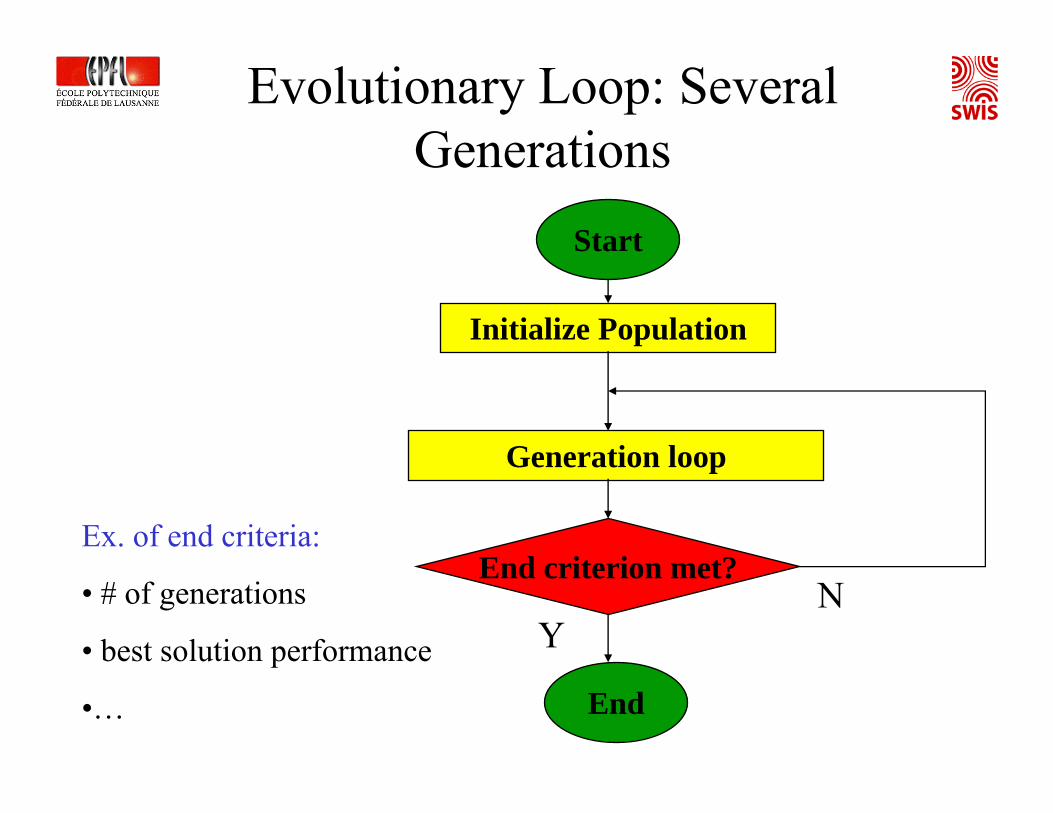
Evolutionary Loop: Several Generations

Initialize Population

Generation loop

End criterion met?

End

Start

NY

Ex. of end criteria:

• # of generations

• best solution performance

•…

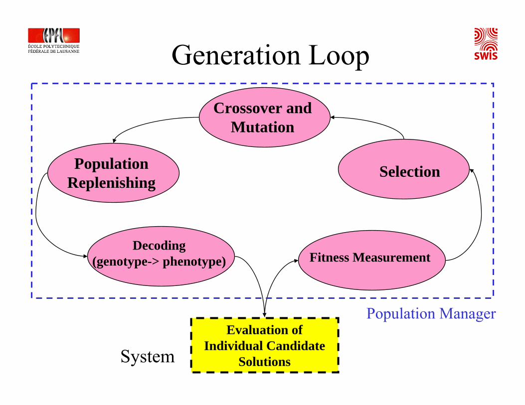
Generation Loop

Evaluation of Individual Candidate

Solutions

Population Replenishing

Selection

Crossover and Mutation

Decoding (genotype-> phenotype)

System

Fitness Measurement

Population Manager

GA: Coding & Decodingphenotype genotype phenotype

coding decoding(chromosome)

• genotype: chromosome = string of genotypical segments, i.e. genes, or mathematically speaking, again a vector of real or binary numbers; vector dimension varies according to coding schema (≥ D)

G1 G2 GnG4G3 … Gi = gene = binary or real number

Coding: real-to-real or real-to-binary via Gray code (minimization of nonlinear jumping between phenotype and genotype)

Decoding: inverted operation

• phenotype: usually represented by a vector of dimension D, D being the dimension of the hyperspace to search; vector components are usually real numbers in a bounded range

Rem:

• Artificial evolution: usually one-to-one mapping between phenotypic and genotypic space

• Natural evolution: 1 gene codes for several functions, 1 function coded by several genes.

GA: Basic Operators• Selection: roulette wheel (selection probability determined by

normalized fitness), ranked selection (selection probability determined by fitness order), elitist selection (highest fitness individuals always selected)

• Crossover: 1 point, 2 points (e.g. pcrossover = 0.2)

• Mutation (e.g. pmutation = 0.05)

Gk Gk’

Note: examples for fixed-length chromosomes!

GA: Discrete vs Continuous• For default GA, all parameters discrete

(e.g., binary bits, choice index)• Common adaptation for continuous

optimization:– Parameters are real values– Mutation: apply randomized adjustment to gene

value (i.e. Gi’ = Gi + m) instead of replacing value

• Selection of adjustment range affects optimization progress

Particle Swarm Optimization

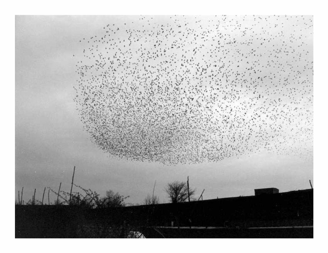
separation

1. Separation: avoid collisions with nearby flockmates

Reynolds’ Rules for Flocking

Position control Position controlVelocity control

2. Alignment: attempt to match velocity (speed and direction) with nearby flockmates

alignment cohesion

3. Cohesion: attempt to stay close to nearby flockmates

More on Week 7

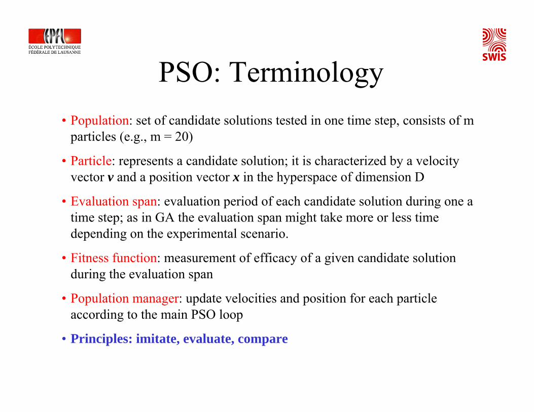
PSO: Terminology• Population: set of candidate solutions tested in one time step, consists of m

particles (e.g., m = 20)

• Particle: represents a candidate solution; it is characterized by a velocity vector v and a position vector x in the hyperspace of dimension D

• Evaluation span: evaluation period of each candidate solution during one a time step; as in GA the evaluation span might take more or less time depending on the experimental scenario.

• Fitness function: measurement of efficacy of a given candidate solution during the evaluation span

• Population manager: update velocities and position for each particle according to the main PSO loop

• Principles: imitate, evaluate, compare

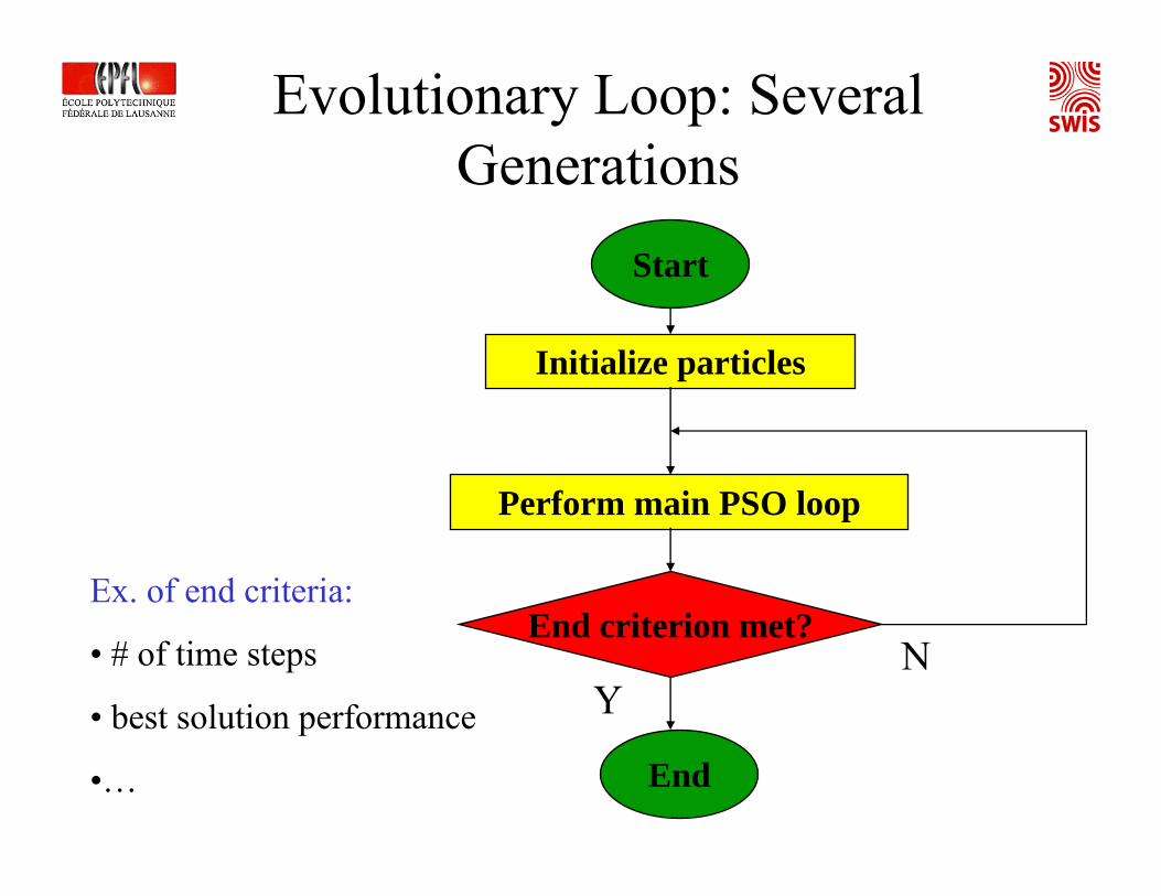
Evolutionary Loop: Several Generations

Initialize particles

Perform main PSO loop

End criterion met?

End

Start

NY

Ex. of end criteria:

• # of time steps

• best solution performance

•…

Initialization: Positions and Velocities

The Main PSO Loop – Parameters and Variables

• Functions– rand ()= uniformly distributed random number in [0,1]

• Parameters– w: velocity inertia (positive scalar)– cp: personal best coefficient/weight (positive scalar)– cn: neighborhood best coefficient/weight (positive scalar)

• Variables– xij(t): position of particle i in the j-th dimension at time step t (j = [1,D])– vij(t): velocity particle i in the j-th dimension at time step t– : position of particle i in the j-th dimension with maximal fitness up to

iteration t– : position of particle i’ in the j-th dimension having achieved the

maximal fitness up to iteration t in the neighborhood of particle i

)(* txij

)(* tx ji′

The Main PSO Loop (Eberhart, Kennedy, and Shi, 1995, 1998)

for each particle i

update the

velocity

( ) ( )1)1( ++=+ tvtxtx ijijijthen move

for each component j

At each time step t

)()()()(

)()1(**

ijjinijijp

ijij

xxrandcxxrandc

twvtv

−+−

+=+

′

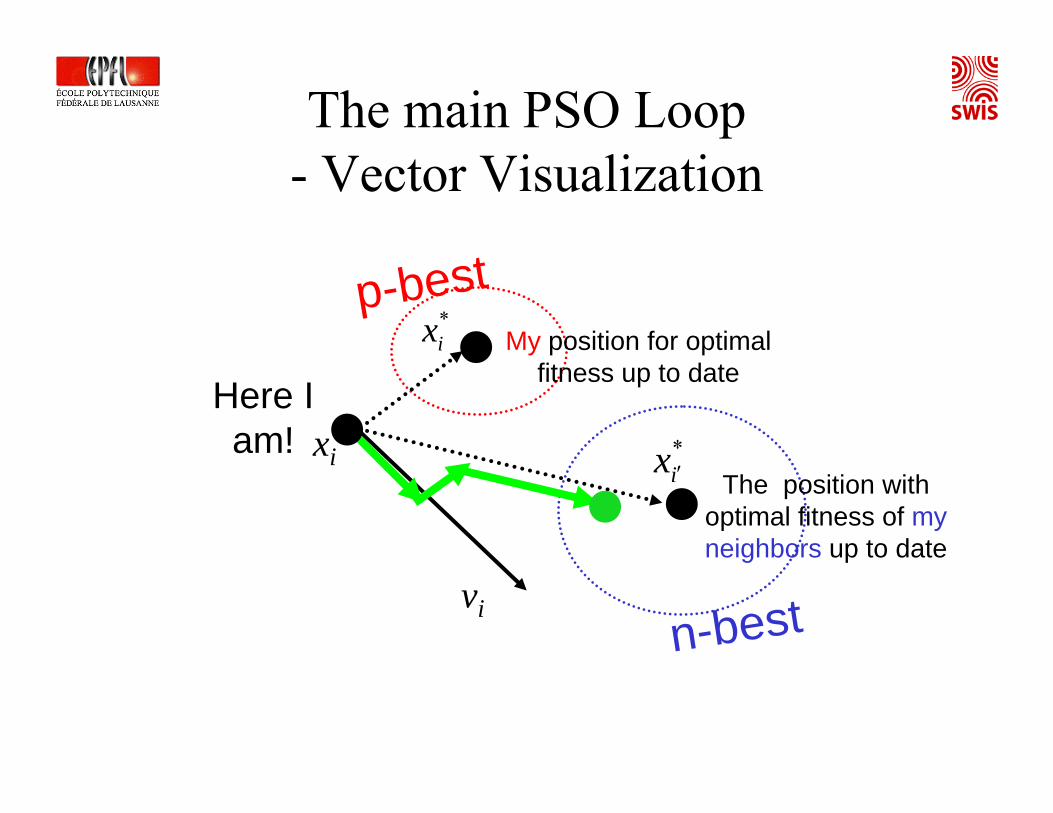
The main PSO Loop- Vector Visualization

*ix

Here I am!

The position withoptimal fitness of my neighbors up to date

My position for optimal fitness up to date

xi

vi

p-best

n-best

*ix ′

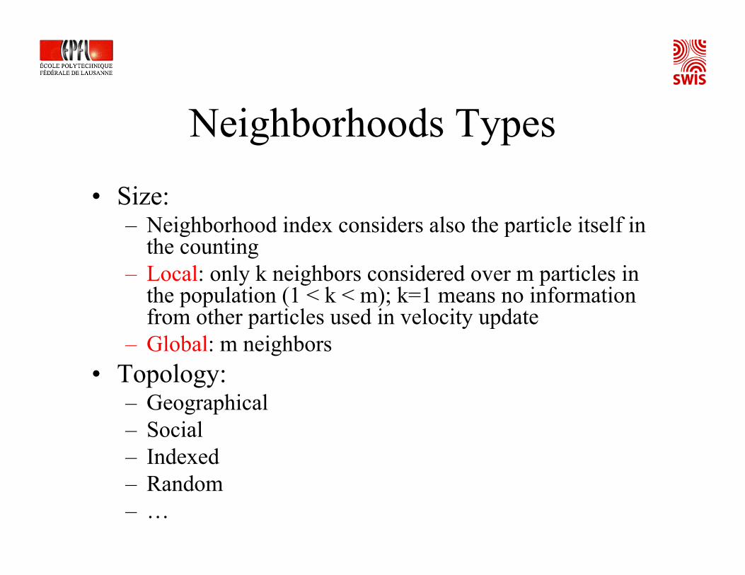
Neighborhoods Types

• Size: – Neighborhood index considers also the particle itself in

the counting – Local: only k neighbors considered over m particles in

the population (1 < k < m); k=1 means no information from other particles used in velocity update

– Global: m neighbors• Topology:

– Geographical– Social– Indexed– Random– …

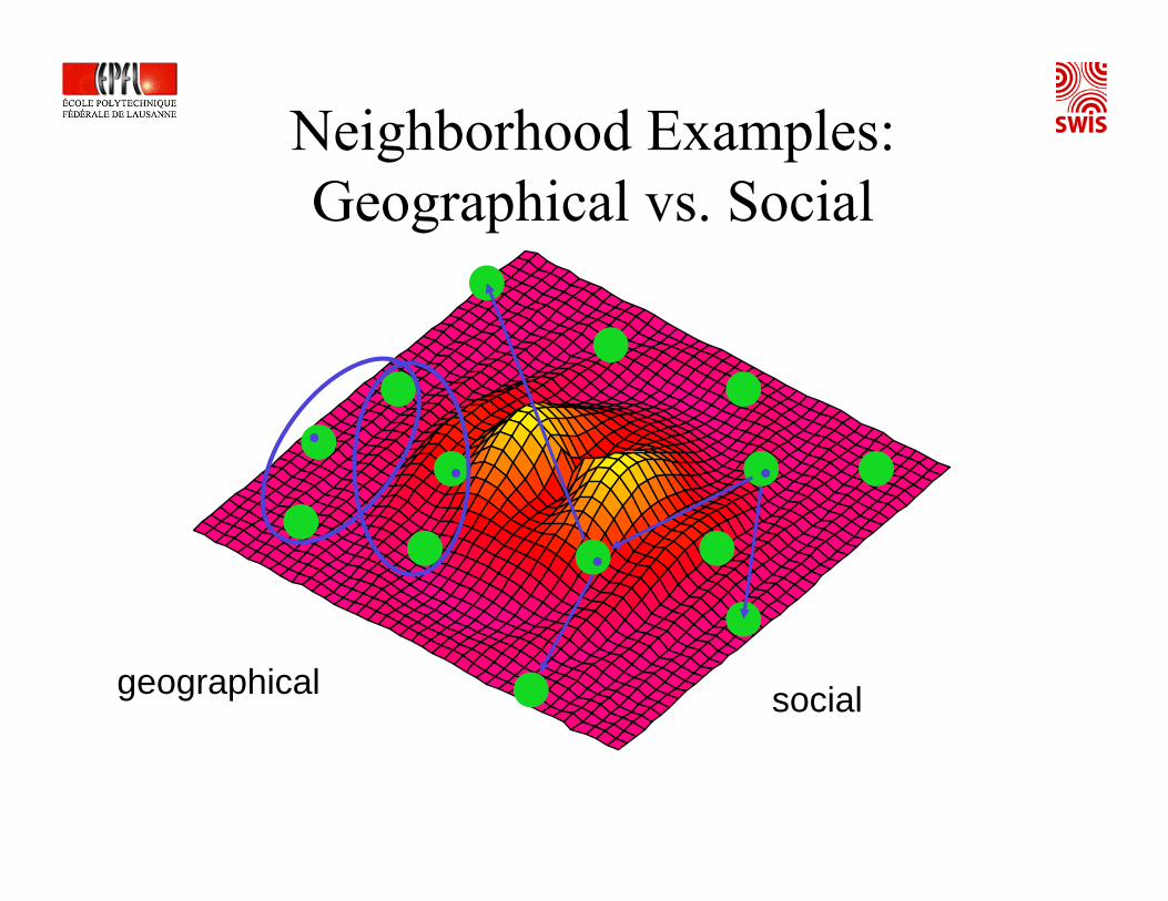
Neighborhood Examples: Geographical vs. Social

geographical social

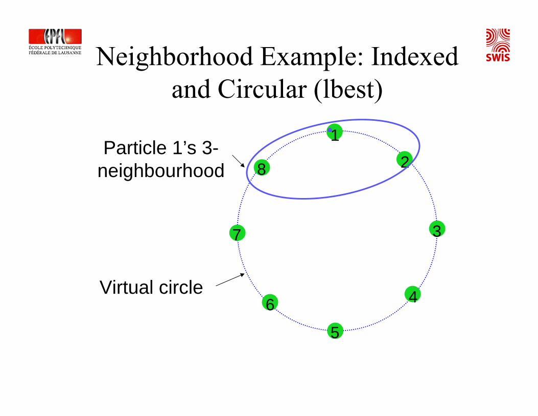
Neighborhood Example: Indexed and Circular (lbest)

Virtual circle

1

5

7

6 4

3

8 2Particle 1’s 3-

neighbourhood

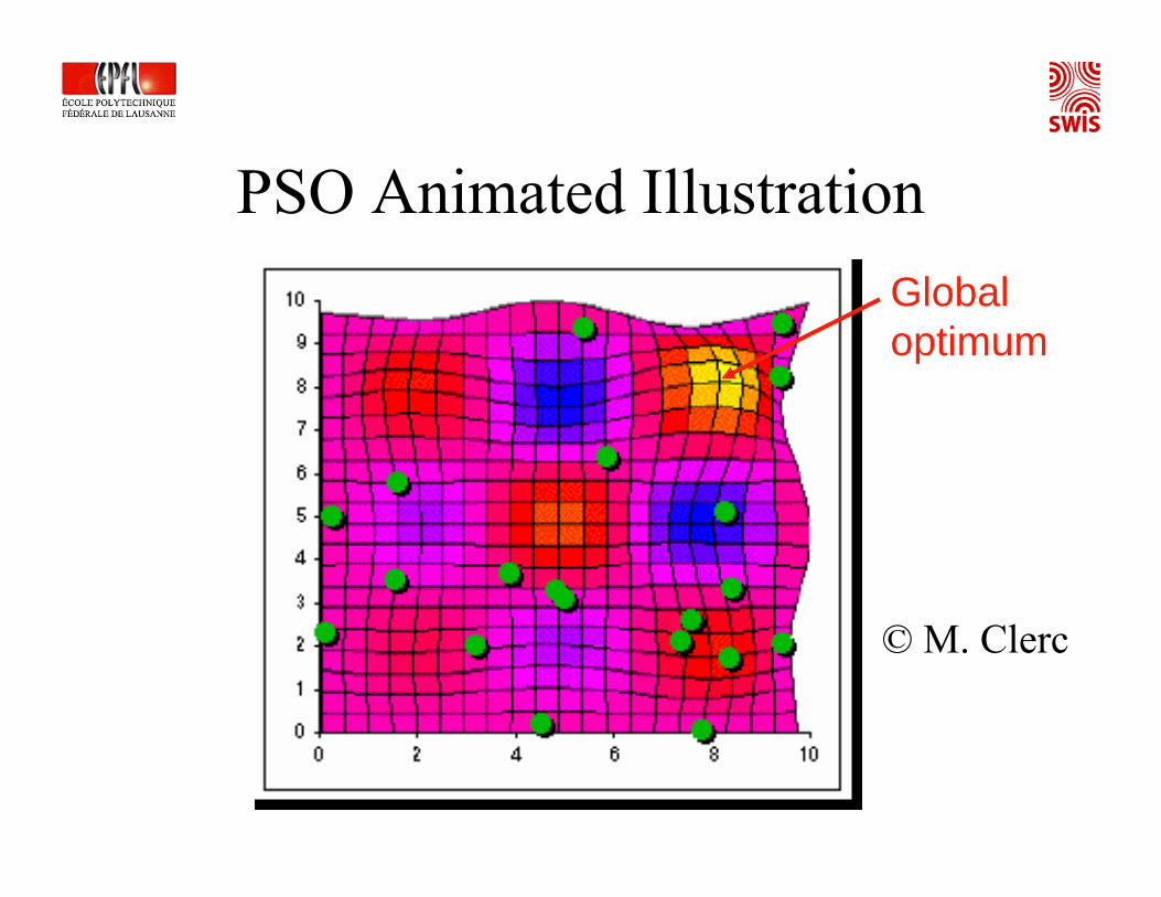
PSO Animated Illustration

© M. Clerc

Global optimum

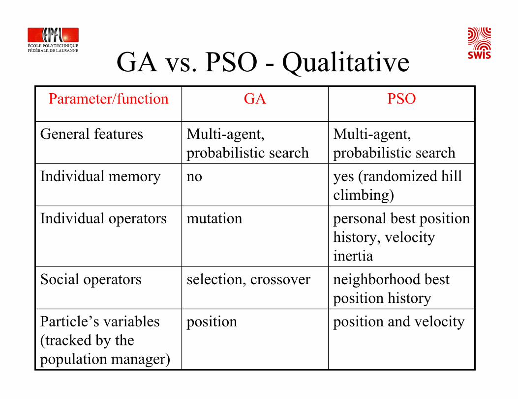
GA vs. PSO - Qualitative

Multi-agent, probabilistic search

Multi-agent, probabilistic search

General features

Particle’s variables (tracked by the population manager)

Social operators

Individual operators

Individual memory

Parameter/function

position and velocityposition

neighborhood best position history

selection, crossover

personal best position history, velocity inertia

mutation

yes (randomized hill climbing)

no

PSOGA

GA vs. PSO - Qualitative

Particle’s variables (tracked by the population manager)

Global/local search balance

Population diversity

# of algorithmic parameters (basic)

Parameter/function

position and velocityposition

Tunable with w (w↑→ global search; w↓→ local search)

somehow tunable via pc/pm ratio and selection schema

Mainly via local neighborhood

somehow tunable via pc/pm ratio and selection schema

w, cn, cp, k, m, position and velocity range (2) = 7

pm, pc, selection par. (1), m, position range (1) = 5

PSOGA

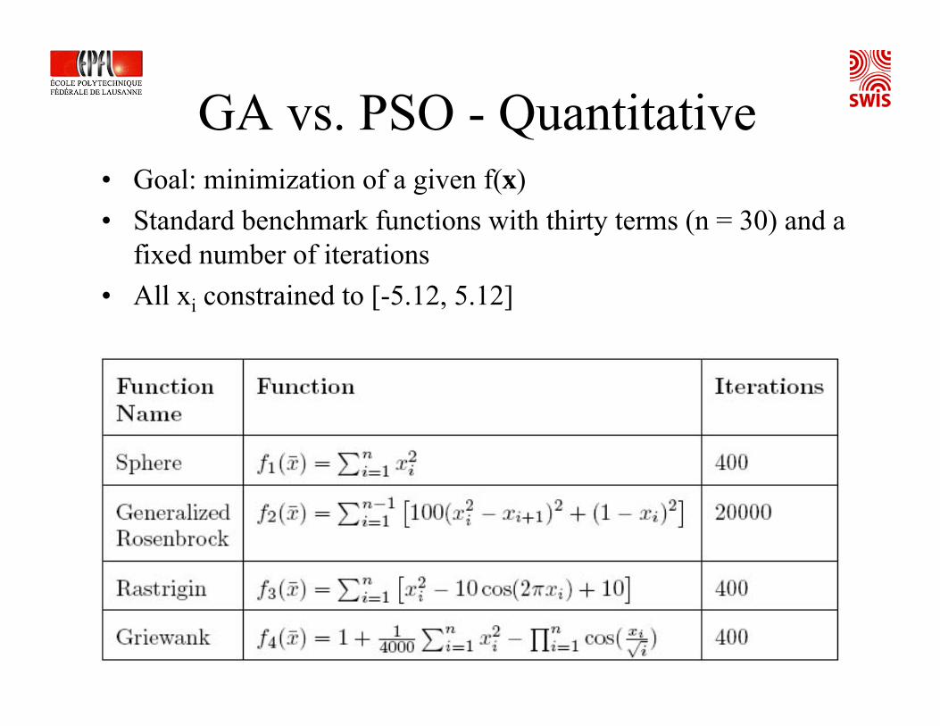
GA vs. PSO - Quantitative• Goal: minimization of a given f(x)• Standard benchmark functions with thirty terms (n = 30) and a

fixed number of iterations• All xi constrained to [-5.12, 5.12]

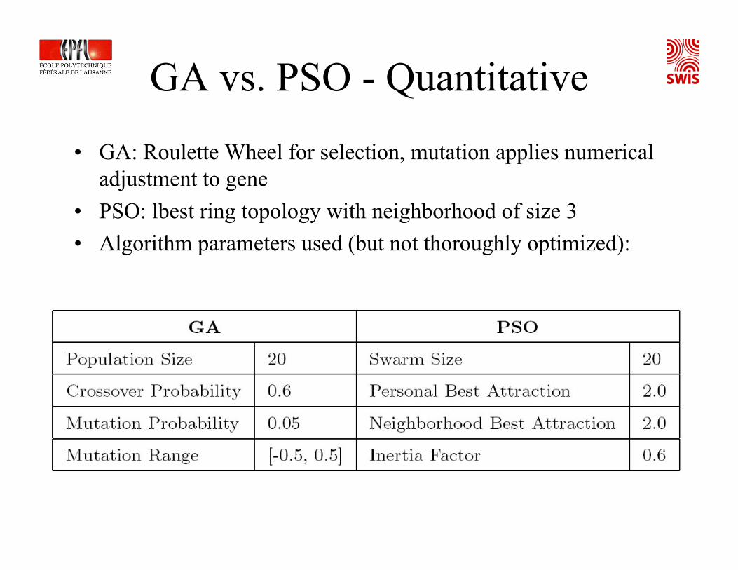
• GA: Roulette Wheel for selection, mutation applies numerical adjustment to gene

• PSO: lbest ring topology with neighborhood of size 3• Algorithm parameters used (but not thoroughly optimized):

GA vs. PSO - Quantitative

GA vs. PSO - Quantitative

0.01 ± 0.030.01 ± 0.01Griewank

48.3 ± 14.4157 ±21.8Rastrigin

7.38 ± 3.2734.6 ± 18.9Generalized Rosenbrock

0.00 ± 0.000.02 ± 0.01Sphere

PSO(mean ± std dev)

GA (mean ± std dev)

Function (no noise)

Bold: best results; 30 runs; no noise on the performance function

GA vs. PSO – Overview• According to most recent research, PSO

outperforms GA on most (but not all!) continuous optimization problems

• No-Free-Lunch Theorem• GA still much more widely used in general

research community• Because of random aspects, very difficult to

analyze either metaheuristic or make guarantees about performance

Conclusion

Take Home Messages

• A key difference in machine-learning is supervised vs. unsupervised techniques

• Unsupervised techniques are key for robotic learning• Two robust multi-agent probabilistic search

techniques are GA and PSO• They share some similarities and some fundamental

differences• PSO is a younger technique than GA but extremely

promising; it has been invented by the swarm intelligence community

Additional Literature – Week 5Books• Mitchell M., “An Introduction to Genetic Algorithms”.

MIT Press, 1996.• Goldberg D. E., “Genetic Algorithms in Search:

Optimization and Machine Learning”. Addison-Wesley, Reading, MA, 1989.

• Kennedy J. and Eberhart R. C. with Y. Shi, “Swarm Intelligence”. Morgan Kaufmann Publisher, 2001.

• Clerc M., “Particle Swarm Optimization”. ISTE Ltd., London, UK, 2006.

• Engelbrecht A. P., “Fundamentals of Computational Swarm Intelligence”. John Wiley & Sons, 2006.