Swarm Intelligence – W6: Application of Machine- Learning...

Swarm Intelligence – W6:Application of Machine-Learning Techniques to Automatic Design and

Optimization of Robotic Systems

Outline• Learning to avoid obstacles

– Machine-learning for ANN shaping– Floreano and Mondada single-robot experiment

• Dealing with noise– Noise-resistant GA and PSO– Pugh et al. systematic study

• Moving beyond obstacle avoidance– Learning of more complex behaviors– HW&SW co-design

• Co-learning in multi-robot systems– Different strategies– Examples

Learning to Avoid Obstacles by Shaping a Neural Network

Controller using Genetic Algorithms

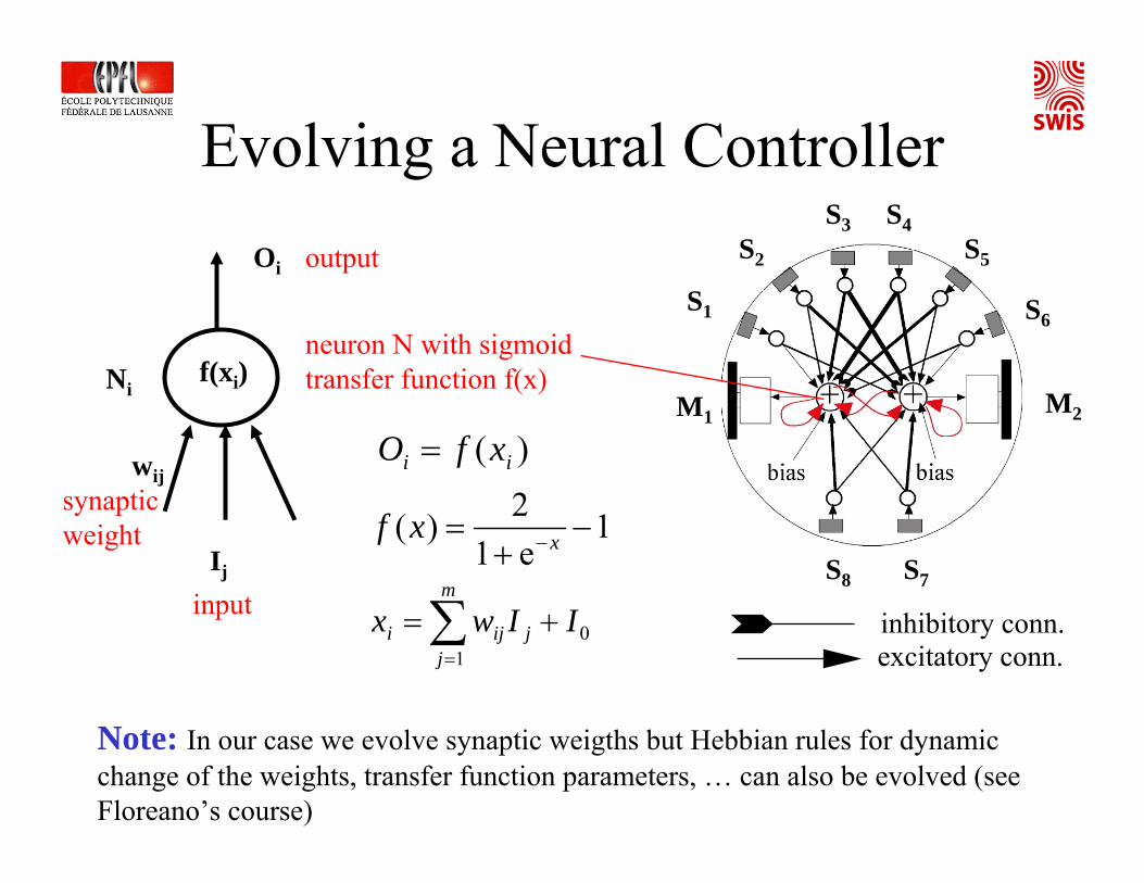
Evolving a Neural Controller

f(xi)

Ij

Ni

wij

1e12)( −+

= −xxf

output

synaptic weight

input

neuron N with sigmoidtransfer function f(x)

S1

S2

S3 S4S5

S6

S7S8

M1 M2

∑=

+=m

jjiji IIwx

10

Oi

)( ii xfO =

inhibitory conn.excitatory conn.

Note: In our case we evolve synaptic weigths but Hebbian rules for dynamic change of the weights, transfer function parameters, … can also be evolved (see Floreano’s course)

Evolving Obstacle Avoidance(Floreano and Mondada 1996)

• V = mean speed of wheels, 0 ≤ V ≤ 1• ∆v = absolute algebraic difference

between wheel speeds, 0 ≤ ∆v ≤ 1• i = activation value of the sensor with the

highest activity, 0 ≤ i ≤ 1

)1)(1( iVV −∆−=Φ

Note: Fitness accumulated during evaluation span, normalized over number of control loops (actions).

Defining performance (fitness function):

Evolving Robot Controllers

Note:Controller architecture can be of any type but worth using GA/PSO if the number of parameters to be tuned is important

Evolved Obstacle Avoidance Behavior

Note: Direction of motion NOT encoded in the fitness function: GA automatically discovers asymmetry in the sensory system configuration (6 proximity sensors in the front and 2 in the back)

Generation 100, on-line, off-board (PC-hosted) evolution

Evolving Obstacle Avoidance

Evolved path

Fitness evolution

Noise-Resistant GA and PSO for Design and Optimization

of Obstacle Avoidance

Noisy and Expensive Optimization

• Multiple evaluations at the same point in the search space yield different results

• Depending on the optimization problem the evaluation of a candidate solution can be more or less expensive in terms of time (i.e. significantly more important than applying the metaheuristic operators)

• Noise causes decreased convergence speed and residual error

• Little exploration of noisy and expensive optimization in evolutionary algorithms, and very little in PSO

Key Ideas• Better information about candidate solution can be obtained by

combining multiple noisy evaluations• We could evaluate systematically each candidate solution for a

fixed number of times → not smart from computational point of view, in particular for expensive optimization problems

• In particular for expensive optimization problems, we want to dedicate more computational time to evaluate promising solutions and eliminate as quickly as possible the “lucky” ones → each candidate solution might have been evaluated a different number of times when compared

• In GA good and robust candidate solutions survive over generations; in PSO they survive in the individual memory

• Use aggregation functions for multiple evaluations: ex. minimum and average

GA PSO

Example: Gaussian Additive Noise on Generalized Rosenbrock

Fair test: samenumber of evaluations candidate solutions for all algorithms (i.e. n generations/ iterations of standard versions compared with n/2 of the noise-resistant ones)

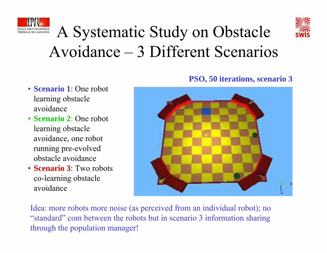
A Systematic Study on Obstacle Avoidance – 3 Different Scenarios

• Scenario 1: One robot learning obstacle avoidance

• Scenario 2: One robot learning obstacle avoidance, one robot running pre-evolved obstacle avoidance

• Scenario 3: Two robots co-learning obstacle avoidance

Idea: more robots more noise (as perceived from an individual robot); no “standard” com between the robots but in scenario 3 information sharing through the population manager!

PSO, 50 iterations, scenario 3

Fitness Function as Before [Floreano and Mondada 1996]

• V = mean speed of wheels, 0 ≤ V ≤ 1• ∆v = absolute algebraic difference

between wheel speeds, 0 ≤ ∆v ≤ 1• i = activation value of the sensor with the


)1)(1( iVV −∆−=Φ

Note: robot(s) essentially the same, environment not (open space with boundary vs. maze) → some of the evolved individuals do straight back and forth movement and achieve high score!

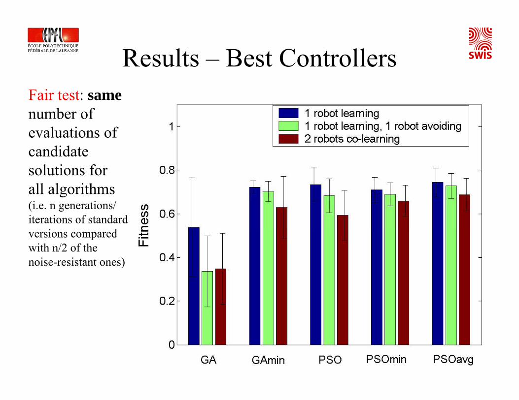
Results – Best ControllersFair test: samenumber of evaluations of candidate solutions for all algorithms(i.e. n generations/ iterations of standard versions compared with n/2 of the noise-resistant ones)

Results – Average ofFinal Population

Fair test: idem as previous slide

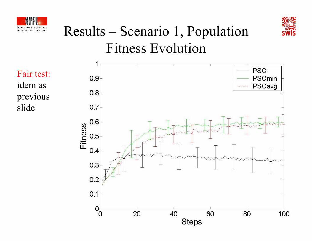
Results – Scenario 1, Population Fitness Evolution

Fair test: idem as previous slide

Not only Obstacle Avoidance: Evolving More

Complex Behaviors

Evolving Homing Behavior(Floreano and Mondada 1996)

Set-up Robot’s sensors

• Fitness function:

• V = mean speed of wheels, 0 ≤ V ≤ 1• i = activation value of the sensor with the


)1( iV −=Φ

• Fitness accumulated during life span, normalized over maximal number (150) of control loops (actions).

• No explicit expression of battery level/duration in the fitness function (implicit).• Chromosome length: 102 parameters (real-to-real encoding).• Generations: 240, 10 days embedded evolution on Khepera.

Controller

Evolving Homing Behavior


Battery energy

Left wheel activation

Right wheel activation

Battery recharging vs. motion patterns

Reach the nest -> battery recharging -> turn on spot -> out of the nest

Evolution of # control loops per evaluation span

Fitness evolution

Evolved Homing Behavior


Activation of the fourth neuron in the hidden layer

Firing is a function of:

• battery level• orientation (in comparison to light

source)• position in the arena (distance

form light source)

Not only Control Shaping: Off-line Automatic

Hardware-Software Co-Design and Optimization

Moving BeyondController-Only Evolution

• Evidence: Nature evolve HW and SW at the same time …

• Faithful realistic simulators enable to explore design solution which encompasses off-line co-evolution (co-design) of control and morphological characteristics (body shape, number of sensors, placement of sensors, etc. )

• GA (PSO?) are powerful enough for this job and the methodology remain the same; only encoding changes

Evolving Control and Robot Morphology

(Lipson and Pollack, 2000)

http://www.mae.cornell.edu/ccsl/research/golem/index.html• Arbitrary recurrent ANN• Passive and active (linear

actuators) links• Fitness function: net distance

traveled by the centre of mass in a fixed duration

Example of evolutionary sequence:

Examples of Evolved Machines

Problem: simulator not enough realistic (performance higher in simulation because of not good enough simulated friction; e.g., for the arrow configuration 59.6 cm vs. 22.5 cm)

From Single to Multi-Unit Systems:

Co-Learning in a Shared World

Evolution in Collective Scenarios

• Collective: fitness become noisy due to partial perception, independent parallel actions

Credit Assignment ProblemWith limited communication, no communication at all, or partial perception:

Co-learning in a Collaborative Framework

Co-Learning Collaborative Behavior

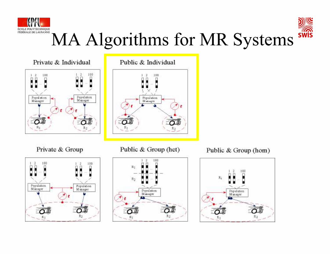
Three orthogonal axes to consider (extremities and balanced solutions are possible):

1. Performance evaluation: individual vs. group fitness or reinforcement

2. Solution sharing: private vs. public policies

3. Team diversity: homogeneous vs. heterogeneous learning

Multi-Agent Algorithms for Multi-Robot Systems

homogeneouspublicgroupg-pu-hoheterogeneouspublicgroupg-pu-hehomogeneousprivategroupg-pr-hoheterogeneousprivategroupg-pr-hehomogeneouspublicindividuali-pu-hoheterogeneouspublicindividuali-pu-hehomogeneousprivateindividuali-pr-hoheterogeneousprivateindividuali-pr-he

DiversitySharingPerformancePolicy

homogeneouspublicgroupg-pu-hoheterogeneouspublicgroupg-pu-hehomogeneousprivategroupg-pr-hoheterogeneousprivategroupg-pr-hehomogeneouspublicindividuali-pu-hoheterogeneouspublicindividuali-pu-hehomogeneousprivateindividuali-pr-hoheterogeneousprivateindividuali-pr-he

DiversitySharingPerformancePolicy

Do not make sense (inconsistent)

Interesting (consistent)

Possible but not scalable

MA Algorithms for MR Systems

Example of collaborative co-learning with binary encoding of 100 candidate solutions and 2 robots


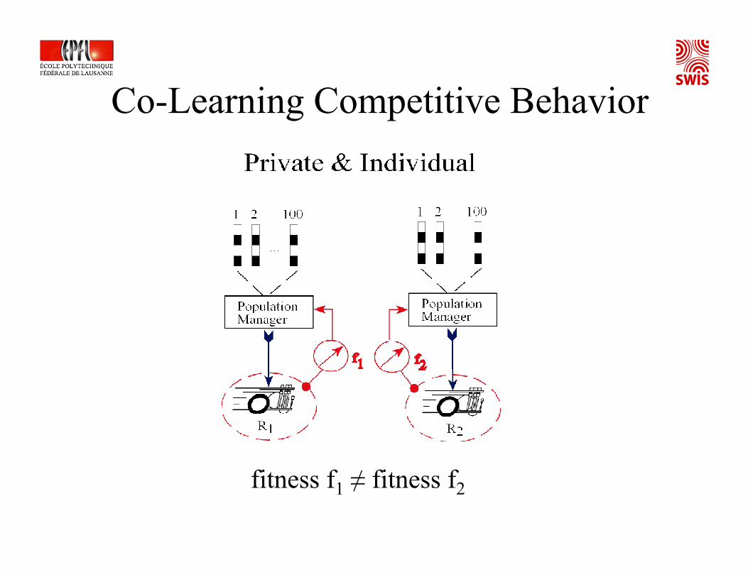
Co-Learning Competitive Behavior

fitness f1 ≠ fitness f2

Co-learning Obstacle Avoidance

• Effects of robotic group size• Effects of communication constraints

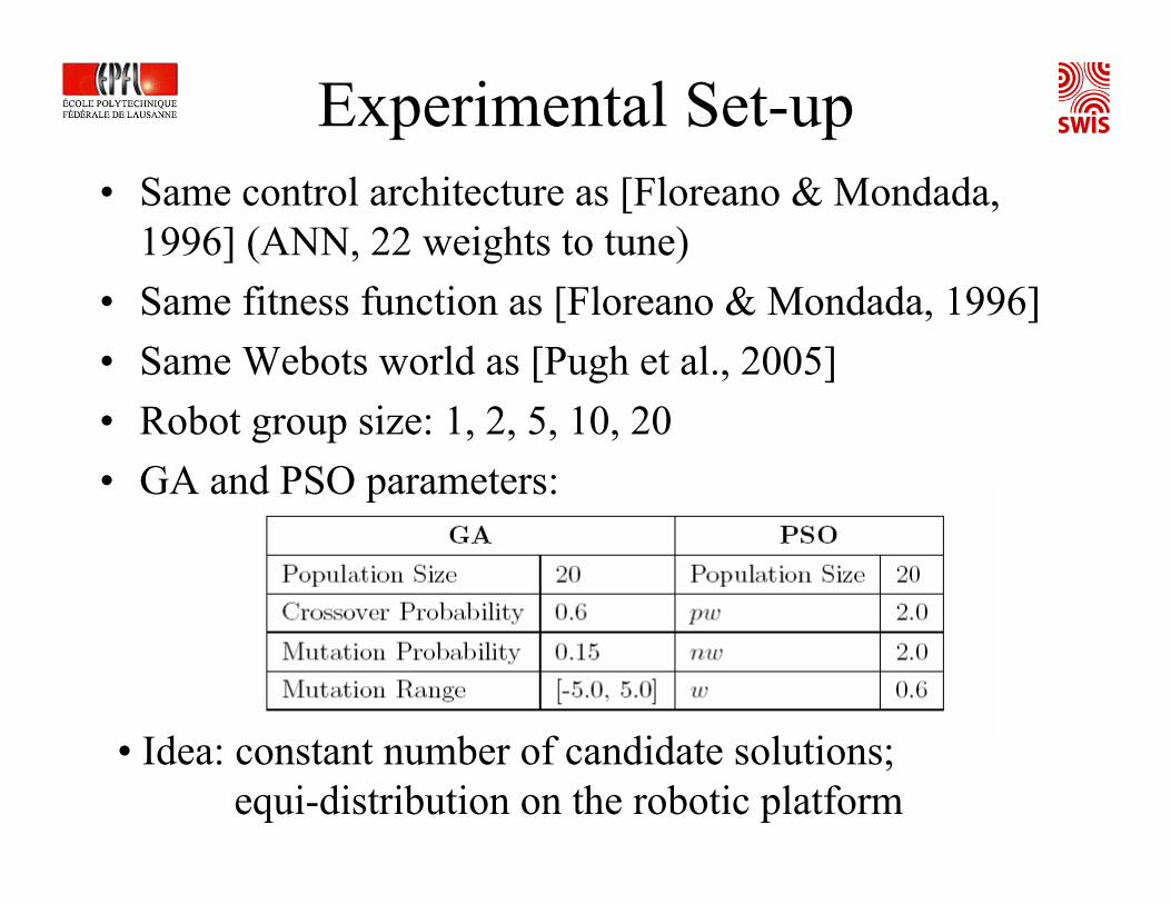
• Same control architecture as [Floreano & Mondada, 1996] (ANN, 22 weights to tune)

• Same fitness function as [Floreano & Mondada, 1996]• Same Webots world as [Pugh et al., 2005]• Robot group size: 1, 2, 5, 10, 20• GA and PSO parameters:

Experimental Set-up

• Idea: constant number of candidate solutions; equi-distribution on the robotic platform

Varying the Robotic Group Size

Varying the RoboticGroup Size - Results

Performance of best controllers after evolution

Communication-Based Neighborhoods

• Default neighborhood - ring topology, 2 neighbors for each robot

• Problem for real robots: neighbor could be very far away

• Possible solutions – use two closest robots in the arena (capacity limitation), use all robots within some radius r (range limitation); reality is affected often by both

• How will this affect the performance?


Ring Topology - Standard


2-Closest – Model 1


Radius r (40 cm) – Model 2

Communication-Based Neighborhoods - Results


Varying Communication Range• Communication range in Model 2

determines expected number of neighbors at each iteration

• How will this affect performance?

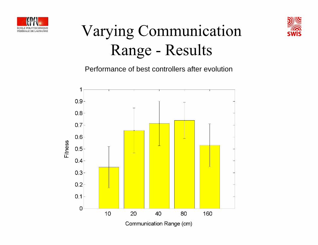
Varying CommunicationRange - Results


Varying CommunicationRange - Results

Average swarm performance during evolution

Co-learning Aggregation

• Effect of the MA-MR mapping policy

Experimental Set-Up

• Same neural network setup as in obstacle avoidance

• Additional capability –sense relative positions of other nearby robots

• Additional inputs to neural network – center of mass (x,y) of detected robots

Fitness Functions

• Individual Fitness Function

• Group Fitness Function (average)

where robRP(i) is number of robots in range of robot i

Note: group fitness quite aligned with individual one

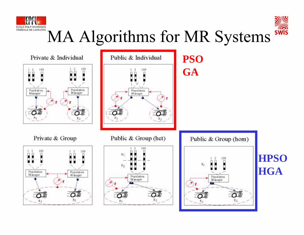
MA Algorithms for MR SystemsPSOGA

HPSOHGA

Sample Results – Strategy Comparison on Best Controllers

Fair test: samenumber of different candidate solution evaluatedon the multi-robot platform(i.e. total evaluation time is the same; e.g. 100 generation GA vs. 5 generations HGA with population size 20)

Sample Results – Strategy Comparison on Population Average

Open question: enough steps for HPSO/HGA?

More Co-learningExperiments

• Coordinated motion of physically connected robots

• Stick-pulling

Information on the SWARM-BOTS project

• A Future and Emerging Technologies project (FET OPEN IST-2000-31010 )

• Started on October 1st, 2001• Lasted 42 months (i.e., ended on March 31,

2005)• Budget: approx 2 millions EUR• Web site: www.swarm-bots.org

CNR, I (S. Nolfi & D.Parisi)CNR, I (S. Nolfi & D.Parisi)

ULB, B (M. Dorigo & J.-L. Deneubourg)ULB, B (M. Dorigo & J.-L. Deneubourg)

ControlControl

IDSIA, CH (L. M. Gambardella)IDSIA, CH (L. M. Gambardella)

SimulationSimulation

HardwareHardware

SWARM-BOTS project partners

QuickTime™ and aTIFF (Uncompressed) decompressor

are needed to see this picture.

QuickTime™ and aTIFF (Uncompressed) decompressor

are needed to see this picture.

EPFL, CH (D. Floreano & F. Mondada)EPFL, CH (D. Floreano & F. Mondada)

What is a swarm-bot?

We call “swarm-bot” an artifact composed of a number of simpler robots, called “s-bots”, capable of self-assembling and self-organizing to adapt to its environmentS-bots can connect to and disconnect from each other to self-assemble and form structures when needed, and disband at will

The coordinated motion task

• Four s-bots are connected in a swarm-bot formation

• Their chassis are randomly oriented

• The s-bots should be able to – collectively choose a direction of

motion – move as far as possible

• Simple perceptrons are evolved as controllers

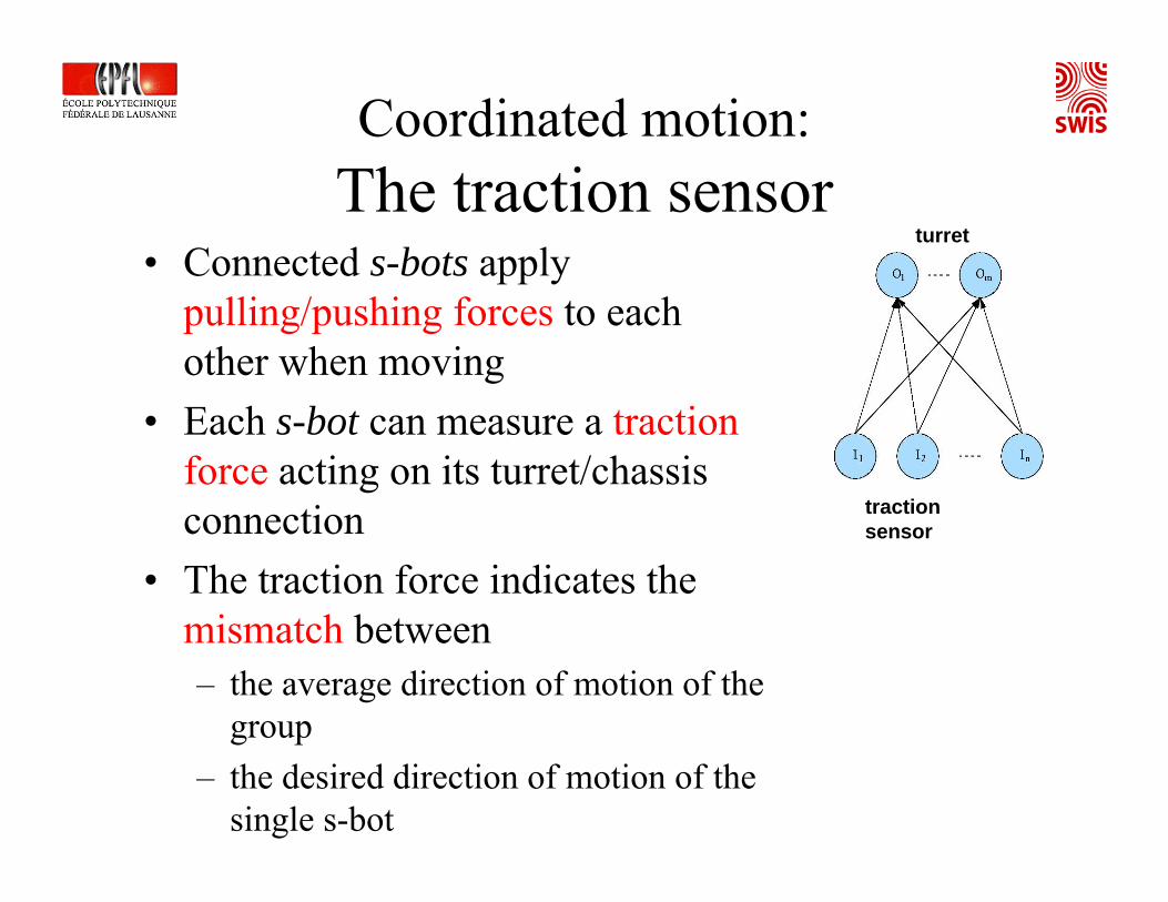
Coordinated motion:The traction sensor

• Connected s-bots applypulling/pushing forces to eachother when moving

• Each s-bot can measure a tractionforce acting on its turret/chassis connection

• The traction force indicates the mismatch between– the average direction of motion of the

group– the desired direction of motion of the

single s-bot

traction sensor

traction sensor

turretturret

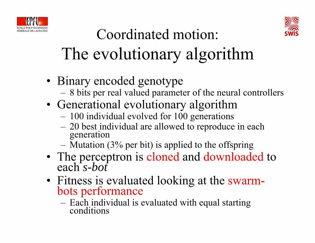
Coordinated motion:The evolutionary algorithm

• Binary encoded genotype– 8 bits per real valued parameter of the neural controllers

• Generational evolutionary algorithm– 100 individual evolved for 100 generations– 20 best individual are allowed to reproduce in each

generation– Mutation (3% per bit) is applied to the offspring

• The perceptron is cloned and downloaded to each s-bot

• Fitness is evaluated looking at the swarm-bots performance– Each individual is evaluated with equal starting

conditions

Coordinated motion:Fitness evaluation

• The fitness F of a genotype is given by the distance covered by the group:

where X(t) is the coordinate vector of the center of mass at time t, and D is the maximum distance that can be covered in 150 simulation cycles

• Fitness is evaluated 5 times (fixed number per candidate solution!), starting from different random initializations

• The resulting average is assigned to the genotype

Coordinated motion: Results

0.76111100.8722290.8584880.8342570.7520960.7957350.7156740.8833830.8395920.878881

PerformanceReplicationAverage fitnessAverage fitness

Post-evaluationPost-evaluation

Coordinated motion: Real s-bots

flexibilityflexibilitydefault (used for evolution)default (used for evolution)

Coordinated motion: Scalability

flexibility and scalabilityflexibility and scalabilityscalabilityscalability

Learning to Pull Sticks

• Homogeneous and heterogeneous learning• Diversity & specialization• Simple in-line adaptive learning algorithm• All applied to the stick-pulling case study

See week 8 lecture: combined agent-based microscopic model with machine-learning method!

Conclusion

Take Home Messages• Unsupervised machine-learning techniques can be

successfully combined with ANN• Both GA and PSO can be used to shape the

behavior by tuning ANN synaptic weights• Computationally efficient, noise-resistant

algorithms can be obtained with a simple aggregation criterion in the main evolutionary loop

• Several successful strategies have been designed for dealing with collective-specific problems (e.g. credit assignment problem)

• The multi-robot platform can be exploited for testing in parallel multiple candidate solutions.

Additional Literature – Week 6Books• Nolfi S. and Floreano D., “Evolutionary Robotics: The Biology, Intelligence, and

Technology of Self-Organizing Machines”. MIT Press, 2004• Sutton R. S. and Barto A. G., “Reinforcement Learning: An Introduction”. The MIT

Press, Cambridge, MA, 1998.

Papers• Lipson, H., Pollack J. B., "Automatic Design and Manufacture of Artificial

Lifeforms", Nature, 406: 974-978, 2000. • Murciano A. and Millán J. del R., "Specialization in Multi-Agent Systems Through

Learning". Biological Cybernetics, 76: 375-382, 1997. • Dorigo M., Trianni V., Sahin E., Groß R., Labella T., Nolfi S., Baldassare G.,

Deneubourg J.-L., Mondada F., Floreano D., and Gambardella L.. “Evolving Self-organising Behaviours for a Swarm-bot”. Autonomous Robots, 17:223–245, 2004

• Mataric, M. J. “Learning in behavior-based multi-robot systems: Policies, models, and other agents”. Special Issue on Multi-disciplinary studies of multi-agent learning, Ron Sun, editor, Cognitive Systems Research, 2(1):81-93, 2001.

• Nolfi S. and Floreano D. “Co-evolving predator and prey robots: Do 'arm races' arise in artificial evolution?” Artificial Life, 4 (4): 311-335, 1999.

• Antonsson E. K, Zhang Y., and Martinoli A., “Evolving Engineering Design Trade-Offs”. Proc. of the ASME Fifteenth Int. Conf. on Design Theory and Methodology, September 2003, Chicago, IL, USA, paper No. DETC2003/DTM-48676.

Swarm Intelligence – W6: Application of Machine- Learning...

Documents

Transcript of Swarm Intelligence – W6: Application of Machine- Learning...