Sustainable Rivers Audit PILOT Project WATER PROCESSES THEME TECHNICAL ... · Sustainable Rivers...
155
Sustainable Rivers Audit Pilot Audit – Water Processes Theme Technical Report i Sustainable Rivers Audit Pilot Project WATER PROCESSES THEME TECHNICAL REPORT Murray-Darling Basin Commission May 2004
Transcript of Sustainable Rivers Audit PILOT Project WATER PROCESSES THEME TECHNICAL ... · Sustainable Rivers...

Sustainable Rivers Audit Pilot Audit – Water Processes Theme Technical Report
i
Sustainable Rivers Audit
Pilot Project
WATER PROCESSES THEME
TECHNICAL REPORT
Murray-Darling Basin Commission
May 2004

Sustainable Rivers Audit Pilot Audit – Water Processes Theme Technical Report
ii

Sustainable Rivers Audit Pilot Audit – Water Processes Theme Technical Report
iii
Foreword The Sustainable Rivers Audit is being developed to benchmark river health across the Murray-Darling Basin and provide information to guide the long term management of riverine resources in the Basin Development of the Audit has been a staged process with the initial focus on obtaining expert advice on the design of an effective Audit. This advice was given effect through establishing a Pilot Audit in four valleys in the Basin: the Ovens in Victoria, the Lachlan in New South Wales, the Condamine in Queensland and the Lower Murray in South Australia. The purpose of the Pilot Audit was to trial the design recommended by the Cooperative Research Centre for Freshwater Ecology encapsulating five thematic sets of indicators: fish, aquatic macroinvertebrates, hydrology, water quality and physical habitat. The Pilot enabled the proposed methods to be evaluated, confirmed the indicators that could be used in a regular Audit and allowed the costs and logistics of a Basin wide Audit to be estimated. This report covers all the technical aspects of the Pilot Audit investigations for the water processes theme. The focus of this report is on method development. However, the resulting river health assessments for the four Pilot valleys are also summarised. The Pilot Audit represents the largest effort in integrated river health monitoring in the Basin to date; with coordinated activity by each of the partner governments utilizing consistent indicators and methods at the same spatial and temporal scales. I believe that the knowledge contained in this and companion documents represent a significant contribution to substantially improving the health of the river systems of the Murray-Darling Basin. Scott Keyworth Director Rivers and Industries Unit May 2004

Sustainable Rivers Audit Pilot Audit – Water Processes Theme Technical Report
iv
Acknowledgments The following people provided input in the technical workshops and working groups: Myriam Bormans (Commonwealth Science and Industry Organisation, CSIRO), Bernard Prendergast (Bureau of Rural Sciences, BRS), Kylee Wilton, Bruce Chessman, Helen Daly, Bruce Cooper and Greg Raisin (New South Wales Department of Infrastructure, Planning and Natural Resources, DIPNR), Klaus Koop, Peter Scanes, Eren Turak, and Geoff Coade (New South Wales Department of Environment and Conservation, DEC) Stuart Bunn and Christie Fellows (Griffith University), Barry Hart and Ian Lawrence (Cooperative Research Centre for Freshwater Ecology, CRCFE), Brian Bycroft and Heather Hunter (Queensland Department of Natural Resources, Mining and Energy, NRM&E), John Bennett and Andrew Moss (Queensland Environmental Protection Authority, Qld EPA), Alieta Donald (Victorian Department of Sustainability and Environment, DSE), David Duncan (South Australian Environmental Protection Authority, SA EPA), Peter Davies (University of Western Australia, UWA), Leon Metzeling and David Robinson (Victorian Environmental Protection Authority, Vic EPA) and Justin Brookes (Cooperative Research Centre for Water Quality Treatment, CRCWQT). The collection of data in the Pilot was undertaken by state agencies in each jurisdiction: Queensland Department of Natural Resources Mining and Energy (NRM&E), the New South Wales Departments of Environment and Conservation, DEC) and Infrastructure, Planning and Natural Resources (DIPNR), the Victorian Environmental Protection Authority (VIC EPA) and Australian Water Quality Centre (AWQC) in South Australia. Four separate reports were commissioned as part of the Pilot. An investigation into the use of chamber methods for routine monitoring purposes was carried out by the following staff from DEC: Danielle Poirier, Jaimie Potts and Max Carpenter (Poirier et al., 2003). Myriam Bormans (CSIRO) reviewed the literature to determine reference conditions for Gross Primary Production, Respiration rates and pelagic Chlorophyll-a levels (Bormans, 2003). Phillip Ford (CSIRO) reviewed the use of stable C and N isotope ratios as an indicator of river health (Ford, 2003), and Stuart Bunn and Christie Fellows (Griffith University) provided a report on the data analysis of stable isotope samples collected during the Pilot project (Bunn and Fellows, 2003). Assistance with the data analysis for spot measurements was provided by Jaimie Potts, Geoff Coade and Peter Scanes, and with graphing of results Joanna Ling and Geoff Gordon (DEC). General development and implementation of the Pilot was guided by the SRA Taskforce, the Commission office project team and the Independent Sustainable Rivers Audit Group (ISRAG). Members of the Taskforce during the Pilot project were: Kylee Wilton (DIPNR), Klaus Koop and Peter Scanes (DEC), Paul Wilson (DSE), Tiffany Inglis and Danny Simpson (South Australia Department of Water Land and Biodiversity Conservation , DWLBC), Brian Bycroft (NRM&E), Terry Loos and Paul Clayton (Qld EPA), Peter Donnelly (Environment ACT), Jean Chesson (BRS), Martin Shaffron and Kylie Peterson (DEH). Members of ISRAG are: Peter E. Davies (Chair), Terry Hillman, Keith Walker and John Harris. The results of the macroinvertebrate theme were documented by the Sustainable Rivers Audit Project Team in this report. Data analysis was undertaken by Wayne Robinson (University of Sunshine Coast, USC) with assistance of ISRAG. The report was primarily written by Frederick Bouckaert with assistance from Project Manager Jody Swirepik and project team members Mark Lintermans, Damian Green and Julie Coysh. Maps were produced by Nick Bauer. Assistance with cover design and print colour quality was provided by Viv Martin. Assistance was also provided by the Bureau of Rural Sciences in compiling the Executive Summary of this report. Draft versions of the report were reviewed by various experts from the Murray-Darling Basin Commission and from relevant state agencies.

Sustainable Rivers Audit Pilot Audit – Water Processes Theme Technical Report
v
Acronyms and abbreviations used in this report ANZECC Australia and New Zealand Environment and Conservation Council ARMCANZ Agriculture and Resources Management Council of Australia and New Zealand AUSRIVAS Australian River Health Assessment AWQC Australian Water Quality Centre, South Australia Basin Murray-Darling Basin BOD Biological Oxygen Demand BRS Bureau of Rural Sciences C Carbon CAP The cap on diversions, agreed to in 1995 Chl-a or Chlor-a Chlorophyll-a CO2 Carbon Dioxide CPOM Course particulate organic material CRCFE Cooperative Research Centre for Freshwater Ecology CRCWQT Cooperative Research Centre for Water Quality Treatment CSIRO Commonwealth Scientific and Industrial Research Organisation DEC Department of Environment and Conservation, New South Wales DEH Commonwealth Department of Environment and Heritage DIBM3 Design and Implementation of Baseline Monitoring report #3 DO Dissolved Oxygen DOC Dissolved Organic Carbon DSE Department of Sustainability and Environment , Victoria EMAP Environmental Monitoring and Assessment Program, from the US Environmental Protection Agency FNARHP First National Assessment of River Health Program FPOM Fine Particulate Organic Material FPZ Functional Process Zone (an area of the river comprised of several reaches with similar geomorphologic
and ecological functions) FPZ’s are aggregated to VPZ’s (see below) GIS Geographic Information System GPP Gross Primary Production ISRAG Independent Sustainable Rivers Audit Group
Expert group of ecologists undertaking the Audit for the SRA program. MDBC Murray-Darling Basin Commission MDBMC Murray-Darling Basin Ministerial Council MRHI Monitoring River Health Initiative N Nitrogen NLWRA National Land and Water Resources Audit NOx Nitrogen Oxides NRM&E Department of Natural Resources, Mines and Energy, Queensland NWQMS National Water Quality Management Strategy O2 Oxygen OM Organic material P Productivity PAR Photosynthetic Active Region Pilot The Pilot project for the Sustainable Rivers Audit Qld EPA Queensland Environmental Protection Authority R Respiration R24 Respiration over a 24 hr cycle SA EPA South Australia Environmental Protection Authority SEPP State Environment Protection Program (Victoria) SRA Sustainable Rivers Audit, also referred to as ‘the Audit’ SR-WI Sustainable Rivers Water Processes index TDS Total Dissolved Solids TOC Total Organic Carbon USC University of the Sunshine Coast UWA University of Western Australia VIC EPA Victorian Environmental Protection Authority VPZ Valley Process Zone: sediment source (upland), sediment transport (slope), sediment deposition (lowland)
zones of a river.

Sustainable Rivers Audit Pilot Audit – Water Processes Theme Technical Report
vi

Sustainable Rivers Audit Pilot Audit – Water Processes Theme Technical Report
vii
Executive summary Murray-Darling Basin water reforms were introduced to improve water use efficiency and to provide protection for aquatic ecosystems across the Basin. The most significant reform, the introduction of the Cap on diversions, sought to balance protection of the riverine environment with the need for consumptive water use. In 2000, the Murray-Darling Basin Ministerial Council (MDBMC) noted the absence of a long-term Basin-wide assessment that could determine the effectiveness of current management practices, including the Cap, in sustaining river health. They agreed to initiate the development of a Sustainable Rivers Audit (SRA) that would assess river health using five themes: macroinvertebrates, fish, water quality, hydrology and habitat. The primary aim of the SRA would be to provide consistent Basin-wide information on the health of rivers (through a rigorous systematic monitoring program) to drive high level, sustainable land and water management decisions. In 2001, the Cooperative Research Centre for Freshwater Ecology developed a framework for assessing the health of the Basin’s rivers with the active involvement of jurisdictional representatives (Whittington et al., 2001). However, before the SRA could be implemented on a Basin-wide scale, it was agreed that a Pilot SRA be conducted in four catchments in 2002/03 (Condamine, Lachlan, Ovens and Lower Murray) to trial and refine indicators and methods, and to identify logistical constraints and indicative costs. The water processes theme intersects between ‘drivers’ (and ‘modifiers’) of river health and ‘outcomes’ of river health, as described by Whittington et al. (2001). Drivers and modifiers are processes that can change river health, while outcomes measure its resulting condition. Water quality is usually regarded as a driver of river health and all the biota living in it. Physico-chemical indicators of water quality characteristics can be seen as ‘drivers’ influencing important ecological processes. However they do not aid the quantification of river processes on the broad temporal and spatial scales proposed by the SRA. Water quality can also be regarded as an ‘outcome’ of health in its own right, a resulting sum total of water inputs, flow and in-stream ecological processes, and as a habitat medium for many organisms. Viewed from this perspective, its role in a river health assessment needs to be made explicit and be distinguished from traditional water quality assessments. This shifts the emphasis to the dynamic ecological processes taking place within the water column. These processes often determine sustainability of the water quality and it is now generally recognised that the focus of measuring in-stream health should be directed towards increasing our understanding of water column metabolic processes. The inclusion of these metabolic processes indicators is therefore considered essential for this theme, and has shifted the emphasis from water quality (‘drivers’) to water processes (‘outcomes’). This report summarises the methods, results and recommendations, focussing on the technical factors, for:
• metabolic rates
• stable isotope ratio measurements
• water quality ‘spot’ measurements which largely contain the traditional water quality parameters.
The costs of implementing any of these groups of indicators in a Basin-wide Sustainable Rivers Audit (SRA) were considered subsequent to these technical considerations and are outside the scope of this report. Cost considerations are presented in the SRA Design report, along with a suggested efficiency rating of all potential Audit components (for instance – fish, macroinvertebrates, physical form etc). The analysis in that report suggests that standard water

Sustainable Rivers Audit Pilot Audit – Water Processes Theme Technical Report
viii
quality indicators (i.e. spot measures) are unlikely to be an efficient input to assessing river health for the SRA. Furthermore, the costs of pursuing metabolic processes are marginal considering the current opinion about how useful the information is to assess river health at the relevant scale. The result is that neither of these components were advocated for inclusion in the first stage of implementation of the SRA. A further consideration was the substantial overlap of a potential water quality/process component of the SRA with existing State water quality monitoring programs. While these existing programs can provide useful information into the Auditing process (possibly to support or interpret assessments based on other indicators), it was not considered appropriate to attempt to make water quality assessments based on current State data programs meet the SRA objectives. The process by which this could happen is yet to be scoped and will depend on the adoption of a Basin-wide Audit. Recommendations are therefore limited to components of this theme that can be incorporated into the SRA without incurring the high costs associated with high intensity field sampling. Further conclusions of the Pilot study are also presented in the event that this theme would be included in a future stage of the SRA.
Design and methods A referential framework has been adopted for the SRA. The aim is to express current river health relative to ‘the condition that would exist now in the absence of human influence experienced during the past two centuries.’ This ‘natural reference condition’ is used to facilitate comparisons across the Basin. Its use does not equate with the objective of returning rivers to a natural condition. Sampling for the Pilot focused on the main river network excluding two important components of riverine ecosystems: aquatic habitats on the floodplain and ephemeral systems. It is expected that these systems will be considered for inclusion in the full SRA given their importance to fish and macroinvertebrate communities. The four river valleys were divided into three valley process zones (VPZ’s) based on geomorphic characteristics: sediment source, sediment transport and sediment deposition. The total number of sites was based on the need for adequate reporting at the valley scale. Results can be reported at finer resolutions but with lower confidence. The number of sites allocated to each zone was based on the area of the zone. Sites were located at random within a zone to ensure that the sampling was unbiased and measurements could therefore be combined to infer the condition of the entire valley. The water processes theme was developed to generate indicators that would enable an assessment of in-stream metabolic processes. The suitability of existing methods for measuring ecological processes - gross primary production (GPP) and respiration (R) were investigated, as was the potential for stable carbon (C) and nitrogen (N) isotope ratios as indicators of river health. Spot measurements of water quality were also included – they were viewed as important ‘drivers’ of change but less informative than process measures (which are ‘outcomes’). Both groups include indicators that are subject to high temporal and spatial variability. Data were collected at approximately 40 assessment sites per valley which generally overlapped with the Pilot Audit fish assessment sites. Although sites are listed in Table 1 as source, transport and deposition, the latter two categories were assumed to behave similarly under base-flow conditions. This was important with regard to the development of reference condition. No ‘best available’ sites were selected for the Murray and Ovens catchments. The sites selected for

Sustainable Rivers Audit Pilot Audit – Water Processes Theme Technical Report
ix
metabolic processes and stable isotope ratios are subsets of the water quality spot measurement sites.
Table 1. Number of sites selected for water quality per VPZ (source, transport, deposition, numbers in italics) and for entire valley (total, best available and assessment), metabolic rates (whole-stream, pelagic and benthic) and stable isotope sampling
Water quality Metabolic rates Stable
Isotopes
Val
ley
Sour
ce
Tran
spor
t
Dep
ositi
on
Tot
al
Tota
l bes
t av
aila
ble
Tota
l as
sess
men
t
Who
le-
stre
am
Pela
gic
Ben
thic
Condamine 12 16 26 54 16 38 9 - - - Lachlan 12 12 36 60 17 43 11 6 4 28 Murray - - 42 42 - 42 - - - - Ovens 21 9 13 43 - 43 12 - - 32 Total 45 37 117 199 33 166 32 6 4 60
Substantive attempts were made to define reference condition for metabolic process indicators (GPP and Respiration), for isotope ratios of δ15N and δ13C of submerged algal and plant material, and for spot measurements (temperature, conductivity, pH, dissolved oxygen, turbidity, total phosphorus, total nitrogen, NOx and chlorophyll-a). The Pilot project aimed to investigate suitable methods for monitoring water processes and characteristics at the Basin scale. At that scale, it proved difficult to define reference conditions for those nine water quality indicators with great confidence. As a result, an assessment of river health was not made against reference and only raw results have been reported. Reference condition values have been presented together with results, but no attempt was made to use these to assess water quality condition. The indicators considered for the water processes theme are listed in Table 2. Indicators related to in-stream processes have the greatest value in increasing our understanding of the in-stream ecology. The Pilot project investigated the use of metabolic process indicator methods and their suitability for routine monitoring purposes on a Basin wide scale. Routine monitoring on a Basin-wide scale for water quality and processes is currently non-existent. Three methods for measuring metabolism rates were trialled: whole-stream metabolism, benthic chambers and pelagic chambers, and their use and compatibility as monitoring tools were discussed on the basis of the experiments, technical problems and results obtained.

Sustainable Rivers Audit Pilot Audit – Water Processes Theme Technical Report
x
Table 2. List of indicators trialled in the Pilot SRA for the Water Processes theme
Indicator / Indicator Type Classification Rate Measures Note: calc = used in calculation of process,
Interp = used in interpretation of process 1 Respiration / Gross Primary Production
1a. Benthic domes 1b. Water column 1c. Total channel
Primary Ecological Process
2 Stream diurnal DO, pH and temperature Primary Ecological Process 3 External Light Modifier, GPP and respiration (calc) Standing Stocks – Spot measures 1 Macrophyte delta C13 and delta N15 Primary Ecological process indicator 2 Pelagic chlorophyll-a Primary Ecological process indicator 3 Phosphorus (TP, FRP) Secondary ecological process indicator
Modifier, GPP (Interp) 4 Nitrogen (TN, NOx, NH4) Secondary ecological process indicator
Modifier, GPP (Interp) Calc Redox (NOx:NH4)
5 Turbidity Secondary ecological process indicator Modifier, GPP (calc)
6 Clarity – PAR extinction, Secchi depth Modifier, GPP (calc) 7 Electrical Conductivity Modifier, GPP (calc) 8 Alkalinity GPP (calc) 9 Temperature Modifier, Total respiration (calc) 10 Instantaneous velocity and flow Modifier, GPP/respiration (calc) and Standardisation to
reference
Results Metabolic rates The whole-stream method shows the greatest potential for developing a routine monitoring tool, despite the inaccuracies with determining re-aeration coefficients, one of the three components in the change of dissolved gas concentration. The accuracy with which the other two components, production (photosynthesis) and respiration can be determined is affected by this re-aeration coefficient. The problems with estimating re-aeration coefficients are greater in the upstream regions than in the lowland areas, due to the higher turbulence and more complex mixing regimes characteristic of those uplands. To some extent greater accuracy can be achieved by using the ‘two-station’ method, but this would be more costly and not directly comparable to a ‘one station’ measurement in a lowland area. Deployment of data loggers in upland areas could also be constrained by shallow depths and fluctuating water levels, especially at base-flow conditions. However, compared to chamber methods the whole-stream method is preferred, due to its relative ease of sampling, lower potential for equipment failure or breakdown and the data collected being an integrated measure of GPP and respiration. A model exists to validate diurnal production and respiration rates (Grace and Harper, 2003), which was used to verify and screen data collected in the Pilot. This model may need further refinement (including defining its limitations) and could be used to develop a routine monitoring protocol. The chamber methods are only measuring parts of the metabolic processes taking place in the water column, and therefore direct comparisons between data collected with the chambers and the whole-stream method are not possible. In contrast to the whole-stream method, exchange rates of

Sustainable Rivers Audit Pilot Audit – Water Processes Theme Technical Report
xi
oxygen between the atmosphere and the water column can be measured fairly accurately in enclosed chambers, but there are possible distortions of the metabolic processes due to light fractionation and reduction within the chambers. The distortions and the limits imposed by the enclosures mean that measured rates do not necessarily reflect what is happening in the surrounding water column. Benthic and pelagic chambers only measure certain aspects of total metabolic processes and cannot be compared directly. Comparisons between chambers and whole-stream methods reveal that chambers consistently underestimate metabolic rates, but the proportion of underestimation can vary considerably, making calibration between both methods problematic (Poirier et al., 2003). Reference conditions were developed for GPP/R ratios and include a decision tree model (Bormans, 2003). Although these reference conditions can be used to assess stream condition, it is not clear whether it would be useful to make a cross-Basin assessment. Therefore, it is recognised that reference condition will need to be refined further before valid assessments and cross-valley comparison of condition can be made.
Stable isotope ratio measurements Stable carbon (C) and nitrogen (N) isotope analysis of in-stream vegetation (vascular plants and filamentous algae) has been trialled in the Pilot project as indicators of river health. Stable nitrogen isotopes have been used as tracers of anthropogenic sources of nitrogen in aquatic ecosystems, while stable carbon isotopes have been used in identifying sources of organic carbon that support food webs. During the Pilot project, a number of samples of algal and vascular plant material were collected from the streambed at sites sampled for other water quality indicators within the Condamine, the Lachlan and the Ovens catchments during spring 2002 and summer 2003. The material was collected according to the protocols developed for the Pilot project (APPENDIX 3) and the samples were analysed by mass spectrometry for stable C and N isotope ratios. The results indicate that considerable variation in stable nitrogen (and carbon) isotope signatures was found among samples of aquatic plants in river sites in NSW and Victoria, collected in the SRA Pilot. δ15N values for the Lachlan ranged from –6.2 to 13.3 ‰ and those for the Ovens ranged from –1.1 to 12.2 ‰. The high level of variation in isotope values recorded among ‘replicate’ samples within sites/times is associated with a broad range in ‰ C and N values. This, together with the noted variety of plant samples processed in the laboratory suggests that a wide range of material was collected, including filamentous algae, N-fixing biofilms and emergent C4 macrophytes. Although the Pilot study has highlighted some strong evidence of correlations between land use and N isotope signatures, this work is in a preliminary stage and will need further development before the inclusion of isotope ratios as an indicator can be considered. This indicator would potentially be useful in establishing the relationship between land and water interactions with regard to modification of nutrient cycles. The C isotope ratio has the potential to be used as an indicator of river health, but further research is needed to establish if confounding factors can be eliminated. C isotope ratios can be used as a check on extreme values of GPP, and may be a useful aid in developing methods for accurate GPP measurement. The collection of primary consumers has the potential for integrating these indicators over different time scales. Collection and analysis of the data can be done at low cost, but training is required to ensure quality assurance of the data collected in the field.
Water quality spot measurements Water quality indicators may be regarded as ‘diagnostics’ to explain river health condition if they can capture ‘driver’ mechanisms, but their explanatory value is likely to be limited by the ability

Sustainable Rivers Audit Pilot Audit – Water Processes Theme Technical Report
xii
of the sampling design and frequency of the program to capture trends for indicators with small and/or variable temporal scales. Water quality sampling sites for the Pilot project were selected and sampled according to a protocol agreed upon during the initial technical workshop and involved a limited number of ‘best available’ sites and a larger number of assessment sites. These sites are a subset of fish and/or macro invertebrate sampling sites and the sampling was undertaken during base-flow conditions. Samples were collected during winter 2002 (limited sites), spring 2002 and summer 2003. Data were collected and substantive attempts made to define reference condition for nine water quality indicators: temperature, conductivity, pH, dissolved oxygen (DO), turbidity, total phosphorus, total nitrogen, NOx and chlorophyll-a. The results of nine indicators are presented in the report for best available sites and assessment sites. Spot measures of physico-chemical indicators can have interpretive value for several of the SRA themes, including the metabolic processes indicators. Defining reference condition for water quality spot measurements would need to be determined and refined before the first assessment of river health condition could be conducted. This would need to be done for all Basin valleys, and would require a coordinated approach. The confidence levels in reference condition of ‘natural’ may be limited and difficult to quantify, due to the difficulties in using best available sites and in limited data being available. However, as more information and data become available, reference condition can be tighter defined and informing on targets may become possible over time. Reporting against targets and on long-term trend detection would gain importance over time and gradually replace assessment against reference condition.
Recommendations As a result of the water processes theme not being recommended for inclusion in the SRA, only three main recommendations have been formulated:
1. A water quality assessment (including GPP, R and Chlorophyll-a) be included in the Remote Sensing Pilot Study objectives which will be undertaken as part of methods development for floodplain assessment, riparian vegetation and physical form. Part of the field verifications and calibrations undertaken for the other themes could include water quality measurements, perhaps by telemetry.
2. ISRAG to develop guidelines for assessing:
a. interpretive datasets from State and other programs, including nutrient budget models (Young et al., 2001 and Prosser et al., 2001) and equilibrium models (Lawrence, 2002)
b. water quality data to be collected as part of SRA fish and macroinvertebrate sampling, to assist in the interpretation of data collected for biotic themes for the SRA.
3. The SRA to keep a watching brief over research related to metabolic processes and the development of GPP/R24 as a routine monitoring tool.
The report also lists a number of conclusions resulting from the Pilot project which could be regarded as recommendations in the event that the water processes theme would be included in the SRA at some point in the future (section 10.2).

Sustainable Rivers Audit Pilot Audit – Water Processes Theme Technical Report
1
TABLE OF CONTENTS
Foreword .....................................................................................................................................................................iii Acknowledgments....................................................................................................................................................... iv
Executive summary ...................................................................................................................................................vii Design and methods.........................................................................................................................................viii Results ................................................................................................................................................................ x Recommendations.............................................................................................................................................xii
1 Introduction........................................................................................................................................................ 2 1.1 Background ................................................................................................................................................ 2 1.2 Purpose of the Audit ................................................................................................................................ 3 1.3 The Pilot SRA.......................................................................................................................................... 5
2 Conceptual basis for theme ............................................................................................................................... 8
3 Aims and development of theme..................................................................................................................... 11 3.1 Aims and objectives ................................................................................................................................. 11 3.2 Theme development process .................................................................................................................... 11
4 Pilot design and construction of reference..................................................................................................... 13 4.1 Variables/indicators measured.................................................................................................................. 17 4.2 Development of conceptual models ......................................................................................................... 19 4.3 Quantifying reference condition............................................................................................................... 24 4.4 Calculation of percentiles for physical indicators and for nutrient data. .................................................. 25 4.5 Confidence in setting reference condition ................................................................................................ 29 4.6 Departure from reference ......................................................................................................................... 30 4.7 Defining reference condition for stable nitrogen isotopes........................................................................ 30 4.8 Defining reference condition for Stable carbon isotopes.......................................................................... 31
5 Metabolic process indicators........................................................................................................................... 32 5.1 Methods.................................................................................................................................................... 32 5.2 Results and discussion.............................................................................................................................. 33 5.3 Power analysis.......................................................................................................................................... 39
6 N & C stable isotope ratio indicators ............................................................................................................. 39 6.1 Background .............................................................................................................................................. 40 6.2 Methods.................................................................................................................................................... 40 6.3 Results ...................................................................................................................................................... 41 6.4 Discussion ................................................................................................................................................ 44 6.5 Power analysis.......................................................................................................................................... 48
7 Water quality spot measurements .................................................................................................................. 49 7.1 Methods.................................................................................................................................................... 49 7.2 Results and discussion.............................................................................................................................. 51 7.3 Power analysis.......................................................................................................................................... 70
8 Assessing all indicators against suitability criteria ....................................................................................... 74
9 Combining indicators into a river health index............................................................................................. 76
10 Recommendations and Conclusions ............................................................................................................... 80 10.1 Recommendations .................................................................................................................................... 80 10.2 Conclusions .............................................................................................................................................. 82
References .................................................................................................................................................................. 85
Appendices .................................................................................................................................................................88 APPENDIX 1 Workshop and technical group participants .............................................................................. 88 APPENDIX 2: GIS map of all NRHMP sampling sites situated within the Pilot valleys for which water quality data were used in determining reference condition (calculation of 20th and 80th percentiles) ........ 89 APPENDIX 3: Pilot sampling protocols........................................................................................................... 90 APPENDIX 4: Sites sampled for water quality spot measurements, metabolic processes and stable isotope plant material. ................................................................................................................................................. 121 APPENDIX 5: Results for water quality spot measurements ......................................................................... 125 APPENDIX 6: Results for benthic and pelagic GPP and R measurements. ................................................... 130 APPENDIX 7: Power analysis on data from assessment sites for each of the spot measurement indicators for Spring and Summer ........................................................................................................................................ 131

Sustainable Rivers Audit Pilot Audit – Water Processes Theme Technical Report
2
1 Introduction
1.1 Background Extensive reforms of the water industry have been introduced across the Murray-Darling Basin to improve efficiency in the way water is used and to provide basic protection for aquatic ecosystems. Recognition of the ongoing deterioration of the riverine environments contributed to the introduction of the Cap on diversions in 1995, seeking to balance protection of the riverine environment with the need for consumptive use of water. The two primary objectives of implementing the Cap were: ‘the need to maintain and, where appropriate, improve existing flow regimes in the waterways of the Murray-Darling Basin to protect and enhance the riverine environment; and, to achieve sustainable consumptive use by developing and managing Basin water resources to meet ecological, commercial and social needs’ (MDBC, 2000). In 2000, the Murray-Darling Basin Ministerial Council commissioned a review of the operation of the Cap, which explicitly identified the need for a broad and comparable assessment of river health across the Basin. Since its introduction, compliance with the Cap had been reported annually, however a Basin-wide assessment of river health had not been undertaken, and consequently no information was available on whether the Basin’s rivers were likely to be sustainable under the Cap. The review highlighted the fact that hundreds of millions of dollars were being spent on initiatives to improve river health but there was no overarching monitoring program to assess the effectiveness of these investments. To address this deficiency, the review recommended a regular ecological Audit for the Basin which over time became known as the Sustainable Rivers Audit (SRA). The Ministerial Council commissioned a scoping study to assess the feasibility of undertaking a Basin-wide assessment of river health (Scope of the Sustainable Rivers Audit, Cullen et al., 2000). In August 2000, Ministerial Council agreed to develop the framework of an Audit with the following broad components or themes: macroinvertebrates, fish, water quality, hydrology and habitat. A jurisdictional Taskforce was established (the Sustainable Rivers Audit Taskforce) to guide the development of the Audit. The CRC for Freshwater Ecology was contracted by the SRA Taskforce to undertake the project ‘Development of a Framework for the Sustainable Rivers Audit’ (Whittington et al., 2001). The development of the Audit framework involved jurisdictional representatives through participation in workshops and where possible review of draft material. The report provided a framework for assessing the health of the Basin’s rivers, recognising that existing State and National programs lack uniformity (and hence the ability to provide Basin-wide inter-valley comparisons), on-going funding commitment and a random sampling design necessary for an unbiased assessment. The objective of the framework was to build as much as possible on existing state programs, and to target a scale and cost that could be realistically considered for ongoing monitoring at a Basin scale. The Framework Report (Whittington et al., 2001) was submitted to Ministerial Council for consideration in August 2001 and it was agreed that a Pilot Audit be undertaken on four catchments. The aim of the Pilot was to trial and refine potential indicators and methods, and to identify indicative costs. Field work was undertaken in 2002-03. This document reports on the outcomes of the water processes theme.

Sustainable Rivers Audit Pilot Audit – Water Processes Theme Technical Report
3
1.2 Purpose of the Audit A broad scale river health monitoring program such as the SRA is an essential tool for the Commission and the partner governments to fulfil statutory obligations, identify the effectiveness of management activities, justify major policy initiatives and identify environmental assets. In addition, consistent information across the Basin is needed to compare river health condition across catchments. However, the current State and National monitoring programs do not allow this as they use a range of different methods and indicators (Whittington et al., 2001). To overcome this limitation, the assessment of river health made by the SRA will adopt a consistent monitoring approach across the Basin and be set up as a surveillance monitoring program to reflect the overall, cumulative impacts of current and past management activities. As such, information from the SRA will complement other programs that examine specific river health issues rather than replace them.
The most significant use of the information from the SRA should be to drive changes in the on ground management of the Basin. This may be in the form of identifying areas for urgent action to stop deterioration, identify areas where new policies or strategies are needed, assist with prioritising funding decisions and assist in identifying assets worthy of protection. In this respect, the SRA is a fundamental tool to underpin the Commissions ICM Policy (which includes setting targets for river health) as well as more specific policies like the Native Fish Strategy and the Cap on diversions.
The Purpose and Principles for the Audit, as presented to the Ministerial Council Meeting 58, on 13th March 2001 are:
Purpose: The SRA will provide consistent, Basin-wide information on the health of rivers to enable and enhance sustainable land and water management by:
• developing a common reporting framework using comparable information, through time and across catchments
• reporting against a consistent and scientifically robust set of river health indicators
• triggering further investigation or action in response to evidence of deteriorating river health
• informing the development of targets for river health, and monitoring of progress towards achieving those targets.
Principles: Most of the current effort in the Basin is on investigative monitoring (monitoring impacts and detection of responses to specific management actions). However, recent experience in the National Land and Water Resources Audit highlights the difficulty in using these defined studies to build any systematic or unbiased picture of river health across catchments and jurisdictions. This is because information from these programs is generally biased towards locations with certain impacts or management relevance, and is often carried out for only a small geographic area or timeframe. To overcome this, one of the primary principles of the Audit will be to use randomly selected sites to enable an unbiased assessment of river condition.
Other principles which have guided the development of the Sustainable Rivers Audit are that it should:
• build upon available information and draw upon activities already being undertaken by partner governments

Sustainable Rivers Audit Pilot Audit – Water Processes Theme Technical Report
4
• use independent auditors with appropriate skills to review information and comment on river health
• report annually to Ministerial Council on the implementation of the SRA to inform discussions on river health
• publicly report audit findings on a regular basis, with assessment and interpretation of indicators at appropriate time-intervals (to be determined)
• compile and report information to assess river health at the river-valley scale, to inform priorities for policy and programs at a Basin scale. (Note that Audit results may trigger a more comprehensive investigation which may inform intra-valley management but State and Territory programs will normally guide intra-valley management).
What the Audit will provide In the short term, the proposed Sustainable Rivers Audit will:
• provide a benchmark for the current condition of river health for each of the river valleys in the Murray-Darling Basin (at the valley and valley zone scale, not at the reach level)
• help identify where investments in natural resource management will provide the greatest benefit
• provide scientific information to inform the community debate on river management processes such as The Living Murray and similar processes in other parts of the Basin related to river management planning or the balance between human use and river health
• set up an overarching framework for Basin wide monitoring and provide impetus for standardisation and integration of monitoring programs across States.
In the longer term, the SRA will:
• provide trend analysis for the selected components of river health so that temporal and spatial comparisons can be made.
• provide information to inform efforts to balance river health and human use.
• inform and assist in the setting of targets for healthy working rivers in the Basin as required under the ICM strategy.
• alter the rate of change, timelines and resources secured to implement management programs and actions
• provide a framework for further expansion of river health assessment to include floodplains, wetlands, estuaries and associated ecosystems
• raise awareness amongst community members, landowners and other stakeholders of the condition and importance of river health by offering access to report results at various spatial levels, and by linking various local initiatives and providing contextual information
It is important to recognise that the Audit will not:
• assess the ecological impacts of any specific management activity or policy (like the Cap) in isolation. The Audit reports on the ecological condition of rivers which is a reflection of all current and past land and water management actions

Sustainable Rivers Audit Pilot Audit – Water Processes Theme Technical Report
5
• replace existing investigative or compliance monitoring for specific activities or operations
• set targets for riverine health. Rather the Audit will supply information for the target setting process by providing an on-going Basin-wide assessment of the current condition of rivers.
1.3 The Pilot SRA The four catchments selected for the Pilot Audit were the Condamine-Culgoa in QLD, the Lachlan in NSW, the Ovens in Victoria and the Lower Murray in SA. These were selected by the states and represent a range of environmental conditions and river types found in the Basin on which the indicators and methods could be tested. Having a Pilot catchment in each major jurisdiction and one located across jurisdictions (the Condamine-Culgoa) also enabled a more realistic assessment of the likely costs and logistical constraints associated with implementation of a Basin-wide Audit.
1.3.1 Aims of the Pilot The intention of the Pilot Audit was to ensure that the Sustainable Rivers Audit would provide an effective and cost efficient assessment of river health consistent across the Basin. The aims of the Pilot as stated in the Project Brief were to:
(1) Provide background information to inform the detail of the audit design by: a. developing reference condition for each of the five themes
b. confirming the criteria for selection of monitoring and reference sites
c. refining and trialling methods for data collection and analysis of indicators
d. providing data to determine the appropriate 'effect size' and hence sample size of individual indices to detect change at the recommended power and confidence level
e. providing data to determine the behaviour of individual indices to ensure that the methods are appropriate to detect recommended differences and that the indicators are sensitive to the likely stressors
(2) Ensure the audit design meets the SRA objectives of comparable and robust information through time and across catchments by:
a. detailing and trialling protocols for data collection, analysis, interpretation, quality control, reporting requirements including timeframes and archiving
b. developing and trialling training programs and procedures
c. developing a protocol for reporting and presenting the data
(3) Develop an information management and communication strategy for reporting Audit results to the ISRAG and to stakeholders.
(4) Trial the implementation and training tasks in each jurisdiction to give a clear indication of the costs of routine auditing and the implications of the reporting intervals.
NOTE: The Pilot was primarily about the development of methods and costings for an ongoing SRA rather than making an assessment of condition of four catchments. This is reflected in the Pilot reports, where there is a strong focus on method development.

Sustainable Rivers Audit Pilot Audit – Water Processes Theme Technical Report
6
1.3.2 Benefits of the Pilot The Pilot was seen as a logical step in implementing the full Audit and had the following benefits:
• Data from the Pilot was used to more thoroughly explore indicators and look for redundancies. For example, does everything that is being measured need to be measured? The Pilot gave the opportunity to trial the indicators recommended in the framework report, which of necessity could not field test its recommendations. The Pilot also allowed investigation of some additional indicators and methods that could not be considered within the constraints that had been set for the Framework Report (Whittington et al. 2001).
• The number of samples required and the frequency of sampling are driven by a number of factors, including the magnitude of the desired detectable change, the confidence in detecting that change, the initial condition score, the variability in the indicator and the reporting scale. While the sample size estimates presented in Whittington et al. 2001 were based on the best information available, a number of assumptions about the behaviour of the indicators had to be made. The Pilot data provided an opportunity to refine the estimates of samples sizes required across the Basin.
• The Pilot has provided an opportunity on a small scale to assemble and in some cases train the technicians required for undertaking the monitoring to an appropriate standard. This has enabled a more accurate costing and a better understanding of the likely logistical issues with implementation of a Basin-wide audit.
• The Pilot has enabled the development and refinement of field techniques and the trial of novel approaches to stream assessment.
• The Pilot has enabled a trial of a range of analysis and reporting techniques which would not otherwise have been possible.
• The Pilot has facilitated the investigation of various approaches to establishing reference condition, an essential part of measuring changes in river health.
• The Pilot enabled the development of a range of implementation options. • The Pilot provided the opportunity to resolve issues identified by Whittington et al.
(2001) as well as implementation issues that were not considered such as the development of methods and protocols for the recommended indicators, site selection, how to deal with ephemeral systems, etc. The Pilot provided an opportunity to reconvene the technical groups for each theme at the start of the Pilot to review the indicators to be trialled and provide guidance on the sampling protocols to be used.
The SRA Taskforce met regularly during the Pilot to manage and co-ordinate jurisdictional implementation and interests. The Independent Sustainable Rivers Audit Group (ISRAG), a group of eminent river ecologists, was convened in September 2001 and also met regularly through out the Pilot. While the main role of the ISRAG is to audit the results of the SRA, they undertook a technical quality assurance role in the Pilot Audit. This essentially ensured that they were comfortable with the Audit instrument they would need to work with for ongoing assessments.
This report discusses the outcomes of the Pilot project’s objectives for water processes, with the exception of a cost analysis which was carried out subsequently. The costs of implementing any of these groups of indicators in a Basin-wide Sustainable Rivers Audit (SRA) were considered

Sustainable Rivers Audit Pilot Audit – Water Processes Theme Technical Report
7
subsequent to these technical considerations and are outside the scope of this report. Cost considerations are presented in the SRA design report, along with a suggested efficiency rating of all potential Audit components (for instance – fish, macroinvertebrates, physical form etc). The analysis in that report suggests that standard water quality indicators (i.e. spot measures) are unlikely to be an efficient input to assessing river health for the SRA. Furthermore, the costs of pursuing metabolic processes are marginal considering the current opinion about how useful the information is to assess river health at the relevant scale. Therefore the recommendations made in this report are limited to components of this theme that can be incorporated into the SRA without incurring the high costs associated with high intensity field sampling. Further conclusions of the Pilot study are also presented in the event that this theme would be included in a future stage of the SRA.

Sustainable Rivers Audit Pilot Audit – Water Processes Theme Technical Report
8
2 Conceptual basis for theme The framework adopted in the Pilot for assessing river health is based on a report by Whittington et al. (2001). For the purposes of the SRA, river health is regarded as synonymous with ecological integrity and is defined as ‘the degree to which aquatic ecosystems support and maintain processes and a community of organisms and habitats with a species composition, diversity, and functional organisation relative to that of natural habitats within a region.’ This definition was subsequently simplified to ‘the degree to which the river supports ecological patterns and processes relative to conditions that have been minimally altered by humans.’ The use of a referential framework in which results are compared to ‘natural’ provides a powerful way of comparing river health in both space and time without requiring a full definition and functional understanding of the components of the ecosystem. The Pilot adopted as the working definition of ‘natural’: ‘the condition that would exist now in the absence of human influence experienced during the past two centuries.’ The use of a natural as a reference does not equate with the objective of returning rivers to a natural condition. While ‘natural’ is by definition the condition with the highest ecological integrity we often accept a departure from natural as necessary for securing other important social and economic values. The conceptual model underlying the Pilot design assumes that if habitat, connectivity and metabolic functioning are maintained in their natural state, then a river’s ecological integrity will be maintained. This model predicts that catchment management has had a significant impact on river health and that the resultant changes will be most clearly quantified by assessing the fish and invertebrate communities, hydrology, water quality and physical habitat. These five themes were recommended in an earlier scoping study (Cullen et al., 2000) that took into account existing programs, methods and data as well as consistency with conceptual models of river function. Other themes such as benthic algae and waterbirds may be appropriate for inclusion in a future, expanded SRA. The indicators developed for these environmental themes can be broadly classified into driver and outcome indices. Driver indicators describe the state of the physical environment and provide a diagnostic function for the condition reported by the biotic and biological process (outcome) indicators. Some physio-chemical indicators such as water quality and habitat can also be outcome indicators when they result from or are significantly modified by biological activity.
In Australia biological assessment of water quality or river health has become more popular in recent years as managers have moved to an ecosystem approach rather than simple compliance monitoring (Norris and Norris, 1995; Norris and Thoms, 1999; Ladson et al., 1999). The aquatic biota is the ultimate ‘end-user’ of river condition and so forms a logical basis for monitoring. Assessment of aquatic biota is an effective means of evaluating non-point source cumulative impacts such as river regulation, habitat degradation and deterioration in water quality (Karr, 1991).
Despite this shift in emphasis, water quality remains an important component of river health, and national monitoring guidelines have been reviewed to include the greater emphasis now being placed on biological monitoring and in-stream ecosystem processes (ANZECC and ARMCANZ, 2000). Investigations into the use of diatoms, algae and stream metabolism are limited to date (Reid et al., 1995; Whitton and Kelly, 1995; Chessman et al., 1999; Bunn et al., 1999) and in-stream ecological processes are still poorly understood. Most biological monitoring to date has concentrated on measuring biotic assemblages (fish and macroinvertebrate communities) as end
Sustainable Rivers Audit Pilot Audit – Water Processes Theme Technical Report
9
points of river health (Simpson et al., 1996; Resh et al., 1995; Chessman, 1995; Growns et al., 1995; Wright et al., 1995).
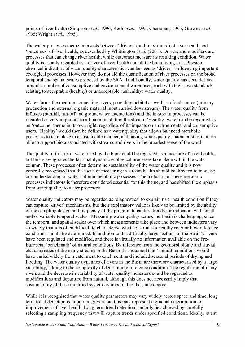
The water processes theme intersects between ‘drivers’ (and ‘modifiers’) of river health and ‘outcomes’ of river health, as described by Whittington et al. (2001). Drivers and modifiers are processes that can change river health, while outcomes measure its resulting condition. Water quality is usually regarded as a driver of river health and all the biota living in it. Physico-chemical indicators of water quality characteristics can be seen as ‘drivers’ influencing important ecological processes. However they do not aid the quantification of river processes on the broad temporal and spatial scales proposed by the SRA. Traditionally, water quality has been defined around a number of consumptive and environmental water uses, each with their own standards relating to acceptable (healthy) or unacceptable (unhealthy) water quality. Water forms the medium connecting rivers, providing habitat as well as a food source (primary production and external organic material input carried downstream). The water quality from influxes (rainfall, run-off and groundwater interactions) and the in-stream processes can be regarded as very important to all biota inhabiting the stream. ‘Healthy’ water can be regarded as an ‘outcome’ theme in its own right, regardless of its impacts on environmental and consumptive users. ‘Healthy’ would then be defined as a water quality that allows balanced metabolic processes to take place in a sustainable manner, and having water quality characteristics that are able to support biota associated with streams and rivers in the broadest sense of the word. The quality of in-stream water used by the biota could be regarded as a measure of river health, but this view ignores the fact that dynamic ecological processes take place within the water column. These processes often determine sustainability of the water quality and it is now generally recognised that the focus of measuring in-stream health should be directed to increase our understanding of water column metabolic processes. The inclusion of these metabolic processes indicators is therefore considered essential for this theme, and has shifted the emphasis from water quality to water processes. Water quality indicators may be regarded as ‘diagnostics’ to explain river health condition if they can capture ‘driver’ mechanisms, but their explanatory value is likely to be limited by the ability of the sampling design and frequency of the program to capture trends for indicators with small and/or variable temporal scales. Measuring water quality across the Basin is challenging, since the temporal and spatial scales over which measurements take place and between indicators vary so widely that it is often difficult to characterise what constitutes a healthy river or how reference conditions should be determined. In addition to this difficulty large sections of the Basin’s rivers have been regulated and modified, and there is virtually no information available on the Pre-European ‘benchmark’ of natural conditions. By inference from the geomorphologic and fluvial characteristics of the many streams in the Basin it is assumed that ‘natural’ conditions would have varied widely from catchment to catchment, and included seasonal periods of drying and flooding. The water quality dynamics of rivers in the Basin are therefore characterised by a large variability, adding to the complexity of determining reference condition. The regulation of many rivers and the decrease in variability of water quality indicators could be regarded as modifications and departure from natural, although this does not necessarily imply that sustainability of these modified systems is impaired to the same degree. While it is recognised that water quality parameters may vary widely across space and time, long term trend detection is important, given that this may represent a gradual deterioration or improvement of river health. Long term trend detection can only be achieved by carefully selecting a sampling frequency that will capture trends under specified conditions. Ideally, event

Sustainable Rivers Audit Pilot Audit – Water Processes Theme Technical Report
10
based monitoring should provide information on peak values which given a certain duration may be critical in influencing river health, but in reality the logistical constraints to event based sampling on such a wide spatial scale cannot be overcome without becoming cost prohibitive.

Sustainable Rivers Audit Pilot Audit – Water Processes Theme Technical Report
11
3 Aims and development of theme
3.1 Aims and objectives The original aim for the water processes theme of the Pilot project was to develop a complete methodology with costings that could be applied across the Basin for the SRA. A technical workshop for the this theme was held in April 2002, reconvening most of the participants involved in earlier workshops run by the CRCFE to develop the Framework report. The recommendations of the Framework report (Whittington et al., 2001) were reconsidered by the group in the light of now having the opportunity to undertake a Pilot project.
The initial workshop identified the following overall aims for the water processes component of the Pilot:
• Further develop the concept of 'reference condition', both ideal and pragmatic definitions.
• Confirm criteria for the selection of sampling sites.
• Conduct a trial Audit at the River Valley and Valley Process Zone scales in the Lachlan, Condamine, Ovens and Lower Murray River valleys.
• Refine and trial data collection methods.
• Refine and trial methods of data analysis and reporting.
• Analyse data with regard to ‘effect size’ and the number of samples required.
• Develop the basis for undertaking a full Sustainable Rivers Audit, including cost estimates and sample timing.
Sampling for water quality and water processes during the Pilot study was aimed at the following specific objectives:
• Examine if sampling a number of water quality and process indicators at base-flow conditions could be used as a reliable indicator of river health
• Use the sampling data to statistically determine an optimum sampling frequency to be recommended for the SRA
• Explore and develop methods for sampling Gross Primary Production and Respiration in an integrated and reliable way, at both upland and lowland sampling sites
• Investigate cost and logistical issues with sampling for this theme
• Determine reference conditions to be used for analysis of Pilot data and for formulating reference condition recommendations
• Develop methods based on reference condition to establish ‘departure from reference’ and to compare river health condition across catchments within the Basin.
3.2 Theme development process The outcomes of the initial workshop (10-11 April 2002) were circulated in the form of proceedings and participants provided further comment out-of-session. The task of compiling suitable sampling protocols was given to Dr. Jane Roberts, and participants were requested to submit field methods for sampling of water processes indicators, who were collated for standardisation and adoption for the Pilot project (APPENDIX 3).

Sustainable Rivers Audit Pilot Audit – Water Processes Theme Technical Report
12
The participating State agencies (Queensland, New South Wales, Victoria and South Australia) subsequently collected water quality information at selected sites according to the protocols developed during the initial technical workshop, and this data was collated by Wayne Robinson (USC) who undertook a preliminary analysis including power analysis and an investigation of compliance and referential approach. The DEC (FORMERLY NSW EPA) was commissioned with investigating the use of benthic chambers as a routine monitoring method for in-stream metabolic processes, and to compare these methods with the diurnal DO methods for which data were collected by all states. The results and analysis of the metabolic processes project have been presented in ‘Water Column and Benthic Metabolism: Review of Concepts and Methods for Monitoring for the Murray Darling Sustainable Rivers Audit (MDBSRA)’ Poirier, D., Potts, J. and Carpenter, M. (2003), and the major findings have been reiterated in this report. CSIRO Land and Water were commissioned with investigating the potential use of stable isotopes as indicators of river health (Potential for the use of the isotopic ratios of Carbon and nitrogen in the SRA monitoring program. Ford, P., 2003), and Dr. Stuart Bunn with data analysis and interpretation of material collected for the stable isotope analysis (Sustainable Rivers Audit Pilot Project: Report on Stable Isotope Indicators. Bunn, S.E. and Fellows, C.S., 2003).
The initial technical reference group appointed a reference reconstruction group to develop reference condition for the water quality and processes indicators which were selected for the Pilot SRA. This reference reconstruction group was smaller but still included members from each state jurisdiction. Several iterations (meetings, teleconferences and out-of-session correspondence) were required by this group to reconstruct reference for most of the indicators for which data were being collected. Reference conditions calculated from the NWQMS (see section 4) needed to be verified against sate monitoring datasets, and for metabolic process indicators CSIRO Land and Water expert Myriam Bormans undertook a literature review to develop reference condition values(Bormans, 2003). A final technical workshop was organised to inform all members of the initial workshop of the developments and outcomes of the Pilot project. Although not all members of the initial workshop were able to be present, the project team ensured that each state jurisdiction was represented at the final workshop, as well as academics with specific expertise. Major outcomes of the Pilot project were considered at the final technical workshop (21 July 2003) where preliminary recommendations on sampling design and determining reference condition were debated and further developed. The contents of this report attempt to reflect the combined views of the range of government and academic experts who have participated in this process. Participants in the workshops and reference reconstruction group are listed in APPENDIX 1 (a,b,c).

Sustainable Rivers Audit Pilot Audit – Water Processes Theme Technical Report
13
4 Pilot design and construction of reference Implicit in the Audit’s assessment of river health is the ability to identify, measure and interpret the key ecological processes and communities in a valley compared to reference. This is difficult in large river systems because ecosystem processes and community structure change along a river from upstream to downstream.
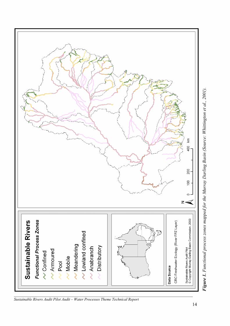
The Pilot Audit adopted a geomorphic approach for stratifying valleys into similar zones at two scales: Functional Process Zones (FPZ’s), Figure 1, and Valley Process Zones (VPZ’s), Figure 2. Functional Process Zones are lengths of a river that have similar discharge and sediment regimes (Thoms, 1998). Their gradient, stream power, valley dimensions and boundary material define them. The characteristics of FPZ’s are summarised in Table 3 and detailed descriptions of the geomorphic characteristics for each of the FPZ’s are outlined in Thoms (1998) and the Framework Report (Whittington et al., 2001). For each FPZ, typically tens to hundreds of kilometres in length, a model of river function describing the key ecosystem processes and structures has been developed (see APPENDIX 2 of Whittington et al., 2001). Functional Process Zones and associated models provided:
• a geomorphic template in which to develop conceptual models of river function
• a basis for identifying VPZ’s, which have been used to stratify sites in the Pilot
• a framework in which to assess the relevance of indicators and reference conditions. Valley Process Zones (VPZ’s) are regions with similar geomorphology within a river valley, identified broadly by their sediment transport characteristics. These are described as regions of sediment source, sediment transport and sediment deposition (see Table 1) and were mapped and defined using FPZ’s1. Most river valleys in the Basin have three VPZ’s, with sediment source regions in the headwaters, sediment deposition regions in the lowlands and the slopes being sediment transport zones. These are mapped in Figure 2. While the original intention of the Audit was to report only at the valley scale, valleys cover such large and diverse geographical areas that significant interest was expressed by the jurisdictions through the Taskforce to report at a finer resolution than the valley scale if that was economically viable. However, more reporting units usually require more sites to be sampled to be able to report with confidence at this finer scale. The VPZ’s were proposed as a suitable finer reporting scale that was still large enough to enable sufficient statistical confidence in most cases without making the number of sites required prohibitive. The Pilot was designed so that all themes could report with a high level of confidence in results at the valley scale, and where possible, at the VPZ scale as well.
1 Repeating units of sediment characteristic (e.g. sediment source, transport, source, etc.) do not allow the strict mapping of FPZ’s into VPZ’s without sometimes having repeating VPZ types in the one river valley. Since VPZ’s are used to stratify the valley for a reporting framework at a broad scale we did not want repeating patterns of VPZ’s. To overcome this, VPZ’s were mapped using the following convention. Mapping started at the bottom of the valley. The FPZ at the bottom of the valley defined the first VPZ. Moving upstream, the first FPZ from the next VPZ became the boundary for that VPZ, and so on. If an FPZ from a downstream VPZ was encountered, this was included in the current VPZ. The outcome of this is that occasionally an FPZ will be allocated to a VPZ of different sediment transport characteristics (e.g. a depositional FPZ in a transport VPZ).
Sustainable Rivers Audit Pilot Audit – Water Processes Theme Technical Report 14
F
igur
e 1.
Fun
ctio
nal p
roce
ss zo
nes m
appe
d fo
r the
Mur
ray
Dar
ling
Basi
n (S
ourc
e: W
hitti
ngto
n et
al.,
200
1).

Sustainable Rivers Audit Pilot Audit – Water Processes Theme Technical Report 15
F
igur
e 2.
Val
ley
proc
ess z
ones
use
d in
the
SRA
(Sou
rce:
Whi
tting
ton
et a
l., 2
001)
.

Tabl
e 3.
Fun
ctio
nal P
roce
ss Z
one
char
acte
risa
tion
(from
Whi
tting
ton
et a
l., 2
001)
Sustainable Rivers Audit Pilot Audit – Water Processes Theme Technical Report 16
P
oo
l U
pla
nd
Go
rge
Arm
ou
red
Mo
bile
Mea
nd
erA
nab
ran
chD
istr
ibu
tary
Lo
wla
nd
go
rge
Va
lley
gra
die
nt/
Lo
ng
p
rofil
e
Va
lley
pro
file
Flo
od
pla
in
fea
ture
s N
o f
loo
dp
lain
N
o f
loo
dp
lain
Min
ima
l flo
od
pla
in
de
velo
pm
en
t. S
om
e
hig
h le
vel t
err
ace
s.
Po
int
an
d la
tera
l ba
rs,
terr
ace
s, in
cise
d
be
nch
es,
fo
rme
r ch
an
ne
ls,
avu
lsio
ns,
flo
od
run
ne
rs
Po
int
an
d la
tera
l ba
rs,
terr
ace
s, in
cise
d a
nd
in
set
be
nch
es,
fo
rme
r ch
an
ne
ls,
avu
lsio
ns,
flo
od
run
ne
rs
Lo
w le
vel
floo
dru
nn
ers
, a
na
bra
nch
ch
an
ne
ls,
ext
en
sive
flo
od
pla
in
Dis
trib
uta
ry
cha
nn
els
F
loo
dp
lain
in
de
pe
nd
en
t o
f m
ain
ch
an
ne
l
Pla
nfo
rmV
alle
y C
on
tro
lled
Sin
uo
sity
= <
1.2
Va
lley
Co
ntr
olle
d
Sin
uo
sity
= <
1.2
S
inu
osi
ty =
1.4
S
inu
osi
ty =
1.4
- 1
.6
Sin
uo
sity
= 1
.6 -
1.8
S
inu
osi
ty =
> 1
.8
Sin
uo
sity
= >
1.8
Va
lley
Co
ntr
olle
d
Sin
uo
sity
= <
1.2
?
Str
ea
m p
ow
er
Lo
w
Lo
w
Lo
w
Mo
de
rate
?
Ve
ry h
igh
H
igh
M
od
era
te
Mo
de
rate
-Lo
w
Do
min
an
t se
dim
en
tsB
ed
rock
, b
ou
lde
r B
ed
rock
, b
ou
lde
r,
cob
ble
C
ob
ble
an
d g
rave
l su
rfa
ce la
yer
pro
tect
ing
p
oo
rly
sort
ed
fin
er
sub
-se
dim
en
ts
Bim
od
al d
istr
ibu
tion
o
f g
rave
l/pe
bb
le a
nd
fin
er
pa
rtic
les
Sa
nd
S
an
d,
silt,
cla
y S
ilt a
nd
cla
y ?
Fu
nct
ion
(se
dim
en
ts,
nu
trie
nts
, o
rga
nic
s)
Ke
y a
qu
atic
h
ab
itats
Re
lativ
ely
imm
ob
ile
sou
rce
are
a
Hig
hly
mo
bile
so
urc
e a
rea
M
ob
ile s
ou
rce
are
a
Mo
bile
tra
nsf
er
are
a
Hig
hly
mo
bile
tra
nsf
er
are
a.
So
me
d
ep
osi
tion
of
fine
r p
art
icle
s
De
po
sitio
nD
ep
osi
tion
dis
trib
uta
ryD
ep
osi
tion
Po
ol,
riff
le c
hu
tes
Riff
le a
nd
po
ol
sub
stra
tum
R
iffle
an
d p
oo
l su
bst
ratu
m,
hig
h f
low
flo
od
run
ne
rs,
rip
ari
an
ve
ge
tatio
n,
sna
gs
Riff
le a
nd
po
ol
sub
stra
tum
, p
oin
t a
nd
la
tera
l ba
rs,
inci
sed
b
en
che
s, f
loo
dru
nn
ers
, w
oo
dy
de
bri
s (s
na
gs)
, m
acr
op
hyt
es
Po
ol s
ub
stra
tum
, p
oin
t a
nd
late
ral b
ars
, fo
rme
r ch
an
ne
ls,
avu
lsio
ns,
in
cise
d a
nd
inse
t b
en
che
s, w
oo
dy
de
bri
s (s
na
gs)
, m
acr
op
hyt
es
Po
ols
, a
na
bra
nch
ch
an
ne
ls,
bill
ab
on
gs,
w
oo
dy
de
bri
s,
ma
cro
ph
tye
s
Po
ol s
ub
stra
tum
, b
illa
bo
ng
s, w
oo
dy
de
bri
s (s
na
gs)
, m
acr
op
hyt
es
Po
ols
,we
tlan
ds
ad
jace
nt
to c
ha
nn
el,
ma
cro
ph
yte
s
Ma
jor
com
po
ne
nts
o
f ca
rbo
n
sup
ply
Allo
chth
on
ou
s in
pu
ts
do
min
an
t: C
PO
M a
nd
F
PO
M,
min
or
pri
ma
ry
pro
du
ctio
n:
mic
roa
lga
e
(dia
tom
s),
som
e
sub
me
rge
d a
nd
e
me
rge
nt
ma
cro
ph
yte
s
Allo
chth
on
ou
s in
pu
ts d
om
ina
nt:
C
PO
M a
nd
FP
OM
, m
ino
r p
rim
ary
p
rod
uct
ion
: m
icro
alg
ae
Allo
chth
on
ou
s in
pu
ts d
om
ina
nt:
C
PO
M,
FP
OM
an
d
log
s, m
ino
r p
rim
ary
p
rod
uct
ion
: p
eri
ph
yto
n
Allo
chth
on
ou
s in
pu
ts:
CP
OM
, F
PO
M a
nd
lo
gs
eq
ua
l pri
ma
ry
pro
du
ctio
n:
em
erg
en
t ve
ge
tatio
n in
po
ols
, p
eri
ph
yto
n
Allo
chth
on
ou
s in
pu
ts:
CP
OM
, F
PO
M a
nd
lo
gs
eq
ua
l pri
ma
ry
pro
du
ctio
n:
sub
me
rge
d a
nd
e
me
rge
nt
veg
eta
tion
in
po
ols
Pri
ma
ry p
rod
uct
ion
d
om
ina
nt:
fila
me
nto
us
alg
ae
an
d
ph
yto
pla
nkt
on
, m
ino
r in
pu
ts o
f C
PO
M,
FP
OM
an
d lo
gs
Pri
ma
ry p
rod
uct
ion
d
om
ina
nt:
fila
me
nto
us
alg
ae
an
d
ph
yto
pla
nkt
on
, m
ino
r in
pu
ts o
f C
PO
M,
FP
OM
an
d lo
gs
Pri
ma
ry p
rod
uct
ion
d
om
ina
nt:
p
hyt
op
lan
kto
n,
min
or
inp
uts
of
CP
OM
, F
PO
M a
nd
lo
gs
Hig
h f
low
Lo
w f
low
Po
ol d
ep
th
incr
ea
ses,
flu
shin
g
flow
s, v
alle
y re
stri
cts
late
ral
con
ne
ctio
n
Po
ol d
ep
th
de
cre
ase
s, n
o
ma
jor
ha
bita
t lo
ss
Rip
ari
an
ve
ge
tatio
n
inu
nd
ate
d,
sco
uri
ng
an
d
flush
ing
flo
ws
Ha
bita
t a
rea
d
ecr
ea
ses
Sm
all
floo
dru
nn
ers
in
un
da
ted
incr
ea
sin
g
ha
bita
t, f
lush
ing
an
d
sco
uri
ng
flo
ws
Ha
bita
t a
rea
d
ecr
ea
ses
Flo
od
run
ne
rs,
inch
an
ne
l b
en
che
s a
nd
te
rre
stri
al
en
viro
nm
en
t in
un
da
ted
in
cre
asi
ng
ha
bita
t a
nd
fo
od
re
sou
rce
s
Riff
les
an
d d
ee
p p
oo
ls,
san
dy
po
int
ba
rs,
em
erg
en
t ve
ge
tatio
n
No
riff
les,
larg
e p
oo
ls,
san
dy
po
int
ba
rs,
em
erg
en
t ve
ge
tatio
n
Flo
od
run
ne
rs,
inch
an
ne
l b
en
che
s a
nd
a
na
bra
nch
es
inu
nd
ate
d
incr
ea
sin
g h
ab
itat
an
d
foo
d r
eso
urc
es
Riff
les,
larg
e p
oo
ls,
san
dy
po
int
ba
rs,
ha
bita
t re
du
ced
to
ma
in
cha
nn
el
Flo
od
run
ne
rs,
inch
an
ne
l b
en
che
s a
nd
a
na
bra
nch
es
inu
nd
ate
d
incr
ea
sin
g h
ab
itat
an
d
foo
d r
eso
urc
es
De
ep
po
ols
an
d
riff
les,
som
e p
oin
t b
ars
, h
ab
itat
red
uce
d t
o m
ain
ch
an
ne
l
Flo
od
run
ne
rs,
inch
an
ne
l b
en
che
s, a
na
bra
nch
es
an
d b
ifurc
atin
g
cha
nn
els
inu
nd
ate
d
Wa
ter
salin
ity in
cre
ase
s fr
om
gro
un
dw
ate
r in
terc
ep
tion
Po
ol d
ep
th
incr
ea
ses,
va
lley
rest
rict
s la
tera
l co
nn
ect
ion
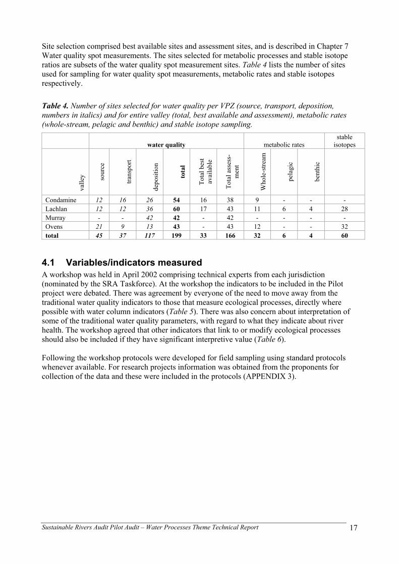
Sustainable Rivers Audit Pilot Audit – Water Processes Theme Technical Report
17
Site selection comprised best available sites and assessment sites, and is described in Chapter 7 Water quality spot measurements. The sites selected for metabolic processes and stable isotope ratios are subsets of the water quality spot measurement sites. Table 4 lists the number of sites used for sampling for water quality spot measurements, metabolic rates and stable isotopes respectively.
Table 4. Number of sites selected for water quality per VPZ (source, transport, deposition, numbers in italics) and for entire valley (total, best available and assessment), metabolic rates (whole-stream, pelagic and benthic) and stable isotope sampling.
water quality metabolic rates stable
isotopes
valle
y sour
ce
trans
port
depo
sitio
n
tota
l
Tota
l bes
t av
aila
ble
Tota
l ass
ess-
men
t
Who
le-s
tream
pela
gic
bent
hic
Condamine 12 16 26 54 16 38 9 - - - Lachlan 12 12 36 60 17 43 11 6 4 28 Murray - - 42 42 - 42 - - - - Ovens 21 9 13 43 - 43 12 - - 32 total 45 37 117 199 33 166 32 6 4 60
4.1 Variables/indicators measured A workshop was held in April 2002 comprising technical experts from each jurisdiction (nominated by the SRA Taskforce). At the workshop the indicators to be included in the Pilot project were debated. There was agreement by everyone of the need to move away from the traditional water quality indicators to those that measure ecological processes, directly where possible with water column indicators (Table 5). There was also concern about interpretation of some of the traditional water quality parameters, with regard to what they indicate about river health. The workshop agreed that other indicators that link to or modify ecological processes should also be included if they have significant interpretive value (Table 6). Following the workshop protocols were developed for field sampling using standard protocols whenever available. For research projects information was obtained from the proponents for collection of the data and these were included in the protocols (APPENDIX 3).

Sustainable Rivers Audit Pilot Audit – Water Processes Theme Technical Report
18
Table 5. Ecological process based indicators considered for inclusion in the Pilot Project. Indicators that will be trialled are given in bold.
Indicators Importance Practicality Confidence in method
Confidence in interpretation
Inclusion in Pilot SRA
Respiration/GPP – benthic, water column, total
H L-M H M YES
Secondary production H L L M NO δC13 plants (shallow, uplands)
M H H L-M YES*
Substrate chlorophyll a (upland)
H H H L NO
Pelagic chlorophyll a (slopes, lowlands)
H H H M YES
Ambient diel DO M M H L-M YES Ambient diel pH M M H L-M YES Microbial prod. -thymidine/leucine uptake
H L L-M L NO
Nutrient cycling δN15 plants M H H L YES* Nutrient spiralling length
M L L-M L-M NO
Algal bioassays (AGP) L-M L H M-H NO** NOx–NH4-TN M H H L YES*** Denitrification with cores
M M M H NO
CPOM-FPOM-DOC (water column)
M L H L NO**
Bioavailable P L L H L NO * as an R&D project ** but should be further explored ***with further review
Table 6. Modifier indicators considered for inclusion in the Pilot Project. Indicators that will be trialled are given in bold. Modifier indicators Supports Inclusion in Pilot SRA Alkalinity Total respiration YES Temperature Total respiration YES pH Total respiration YES Conductivity (TDS) Total respiration YES Flow GPP and respiration YES Turbidity GPP and respiration YES Suspended solids Absorption of nutrients NO NOx-NH4-TN Redox condition, GPP YES Bioavailable P GPP YES Total P GPP YES Benthic/water column redox conditions Diurnal DO and pH NO – covered by NOx-NH4-TN External light GPP and respiration -
benthic YES
Cross section profiles Needed to calculate total GPP/ Respiration
Probably required – could phys habitat theme do them?

Sustainable Rivers Audit Pilot Audit – Water Processes Theme Technical Report
19
4.2 Development of conceptual models The ‘natural’ reference conditions of water processes, including physico-chemical parameters in the water column of various rivers in the Murray Darling Basin during pre-European conditions is largely unknown and undocumented. This is exacerbated by the fact that the timescale during which conditions may change can be relatively short, and that the spatial scale of the Basin is so large that huge variability is likely to exist as a result of a number of Basin characteristics, including:
• altitudinal gradients
• geomorphic variability
• fluctuations in climate, flows and hydrologic regimes
• variations in riparian vegetation and habitat. The large modification of rivers in the Basin since European settlement has confounded the issue. Because of this, it is not possible to reconstruct ‘natural’ reference conditions from historical records; instead it needs to be based on conceptual models, best available sites and expert opinion. Conceptual models developed to explain the ecological dynamics and processes within rivers systems were ‘borrowed’ from Northern Hemisphere river systems (North America and Europe); most remain largely untested for Australian conditions. Although these concepts offer some understanding of the mechanics and processes likely to occur within the water column, known differences between Australian and Northern hemisphere riverine ecosystems warrant a cautious approach. When this information is coupled with data obtained from best available sites (least impacted by anthropogenic uses), and with expert opinion it is considered that reference conditions eventually can be reconstructed as a baseline against which current conditions can be compared. The assumption made in the Framework report (Whittington et al., 2001) that slope VPZ’s would act in a similar way to lowland VPZ’s under base-flow conditions, was adopted and valleys were divided into upland and lowland VPZ’s only (except for the Condamine, where a central VPZ was proposed with specific geomorphologic and water quality characteristics). On the other hand two major issues may drive different models in lowland river zones: flood pulses (the baseline flow conditions assessed after a major pulse) and in-stream productivity. This resulted in the following three models to be considered:
• UPLAND RIVER MODEL (based on the River Continuum Concept), with two variations:
o High Organic Matter input
o Low Organic Matter input
• LOWLAND RIVER: INPUT FROM FLOOD PULSE CONCEPT (based on Flood Pulse Concept)
• LOWLAND RIVERINE PRODUCTIVITY CONCEPT (based on Riverine Productivity Model) The two lowland models characterise different geomorphologies and/or different sources of water (floodplain, channel, and groundwater). Diagrams were developed for each of the models, with descriptors for each of the following:
1. Riparian vegetation
2. Organic matter input

Sustainable Rivers Audit Pilot Audit – Water Processes Theme Technical Report
20
3. Sediments
4. Primary production
5. Chlorophyll-a
6. Flow characteristics
7. Geomorphology
8. Groundwater interaction These descriptors assist in explaining the processes taking place within each model, and in turn would support expert opinion on possible reference values for the listed indicators. It is the intention to develop for each model a table with indicator values (or value ranges) based on data from existing monitoring programs or studies. Figures 3, 4 and 5 explain the three concepts. They are based on diagrams adapted from the Framework report (Whittington et al., 2001) and from the Design and Implementation of Baseline Monitoring (DIBM3) report (Eds. Smith & Storey, 2001). Allocation of a VPZ being made up of predominantly rivers associated with one of the three concepts will require the use of ‘best available sites’ to determine baseline condition, and may require the aid of Physical Form (geomorphology) classification. At present, no reference threshold values for indicators have been developed for each of the models due to lack of more quantitative models.

Sustainable Rivers Audit Pilot Audit – Water Processes Theme Technical Report
21
UPLAND RIVER MODEL
1. Abundant riparian vegetation shades the edges of a stream; GPP and R24 values small, cool temperatures, low
turbidity. 2. For large input of OM: heterotrophic (P<R), net consumer of organic carbon, most nutrients transported
downstream. For small input of OM: autotrophic (P≥ R), net exporter of organic carbon, low nutrient input. 3. Sediment characterised by gravel and cobbles mainly; finer sediments exported downstream and occasionally
accumulated in local pools; riffle areas with fast flow results in high DO and low BOD values. 4. Primary production dominated by biofilms of diatoms and benthic algae. 5. Chlorophyll-a in water column is low due to low nutrient input. 6. First order streams, narrow channels, unidirectional fast flow, low residence time 7. Confined stream channels, with bedrock, gravel and cobbles, limited potential for erosion or sediment
transport. 8. Groundwater interaction: upland streams usually not groundwater fed except at source; interaction unlikely,
but possible in some upland areas; vegetation clearance in surrounding catchment and rising water tables could make this possible. Relative contributions of groundwater to range of indicators determined by surrounding geology, geomorphology and vegetation cover.
Figure 3.Upland River Conceptual Model with 8 descriptions related to structural and functional characteristics.

Sustainable Rivers Audit Pilot Audit – Water Processes Theme Technical Report
22
LOWLAND RIVER: FLOOD PULSE
CONCEPT
1. Limited riparian vegetation fringing a much wider river channel, limiting water shading; higher water
temperatures. 2. CPOM input: large debris from riparian vegetation and organic matter from overland flow and lateral flood
pulses. GPP and R large with R> GPP, heterotrophic system 3. Sediments characterised by sand and clay; finer particles transported downstream and from lateral flood
pulses, occasional upwelling, drying and rewetting resulting in adsorption and nutrient release into the water column
4. Primary production limited by high turbidity, mainly pelagic algal growth in upper water column 5. Chlorophyll-a values low to medium, but highly variable, depending on turbidity and flood pulse regime 6. ‘Unmodified’ lowland stream channel, wide, with wetting and drying cycles and lateral flood pulses,
residence time long but also variable. 7. Broad river channel, with localised pools, sandbars. Sandy and muddy sediments and potential for erosion
and deposition high. 8. Streambed characteristics allow for groundwater interaction, depending on local water table and aquifer
storages. Conductivity is an indicator of this flow pathway.
Figure 4. Lowland river: Flood Pulse Concept with 8 descriptions related to structural and functional characteristics.

Sustainable Rivers Audit Pilot Audit – Water Processes Theme Technical Report
23
LOWLAND RIVERINE PRODUCTIVITY CONCEPT
1. Limited riparian vegetation partly submerged, low sedges and shrubs, shading of water insignificant; water
temperatures cool to warm, depending on number, type and location of modification structures and subsequent flow release.
2. Lateral OM input insignificant, some transported from upstream. High nutrient inputs from upstream and surrounding land use sources. GPP and Respiration large, with GPP > R, autotrophic system.
3. Sediment characterised by fine clays to sand, with capacity to lock up and release nutrients and inorganic pollutants, depending on conditions of pH, temperature, hardness, etc
4. Primary production benthic, pelagic and biofilms; high due to unlimited light, high nutrients and generally low turbidities.
5. High chlorophyll-a values, potential for algal blooms. 6. Flow from wide main-stream channel, limited lateral input, long residence times and slow flows. 7. Broad river channel, fairly stable stream banks and slow flow, silt deposits 8. Groundwater interaction/source possible. For inland lowland river valleys conductivity may be a good
indicator (not in estuaries).
Figure 5. Lowland Riverine Productivity Concept with 8 descriptions related to structural and functional characteristics.

Sustainable Rivers Audit Pilot Audit – Water Processes Theme Technical Report
24
4.3 Quantifying reference condition In absence of quantitative models being available, the reference reconstruction group (APPENDIX 1) investigated the possibility of using data from best available sites for determining reference. The group started by considering which of the indicators (Table 7), used to collect data during the Pilot Project would require reference condition for determining water quality condition. Reference conditions were required for all indicators, adopted for the Pilot project, except for some indicators used in calculation of process (external light, clarity, alkalinity, instantaneous velocity and flow). Initially data and conceptual models were explored from existing monitoring programs; this resulted in the indicators being grouped into the following categories (also see Table 8):
• Physical
• Gross Primary Production (GPP)
• Nutrients/Chlorophyll-a
Table 7. List of indicators trialled in the Pilot SRA for the Water Processes theme. INDICATOR / INDICATOR TYPE CLASSIFICATION Rate Measures Note calc = used in calculation of process,
Interp = used in interpretation of process 1 Respiration / Gross Primary Production
1a. benthic domes 1b. water column 1c. total channel
Primary Ecological Process
2 Stream diurnal DO, pH and temperature Primary Ecological Process 3 External Light Modifier, GPP and respiration (calc) Standing Stocks – Spot measures 1 Macrophyte delta C13 and delta N15 Primary Ecological process indicator 2 Pelagic chlorophyll-a Primary Ecological process indicator 3 Phosphorus (TP, FRP) Secondary ecological process indicator
Modifier, GPP (Interp) 4 Nitrogen (TN, NOx, NH4) Secondary ecological process indicator
Modifier, GPP (Interp) Calc Redox (NOx:NH4)
5 Turbidity Secondary ecological process indicator Modifier, GPP (calc)
6 Clarity – PAR extinction, Secchi depth Modifier, GPP (calc) 7 Electrical Conductivity Modifier, GPP (calc) 8 Alkalinity GPP (calc) 9 Temperature Modifier, Total respiration (calc) 10 Instantaneous velocity and flow Modifier, GPP/respiration (calc) and Standardisation to
reference
Table 8. Indicator categories used to define reference condition Indicator category Indicators Physical pH, Conductivity, DO, Temperature, Turbidity Gross Primary Production GPP, R24 Nutrients/Chlorophyll-a NOX, NH4, TN, TP, FRP, δ13C, δ15N, Chlorophyll-a

Sustainable Rivers Audit Pilot Audit – Water Processes Theme Technical Report
25
Reference condition was defined as a range of values with upper and lower bounds. If a value measured for an indicator would fall outside of these bounds then this could be considered departure from reference. Magnitude of departure needs to be discussed in the context of aggregating the data up to the VPZ level; individual sites are considered replicates and hence site condition assessments are not undertaken. For the physical indicators, it was decided to use tables with 20-80 percentile ranges for upland and lowland sites for setting reference conditions to analyse the Pilot data, analogue to the methodology developed for the National Water Quality Management Strategy (ANZECC and ARMCANZ, 2000)2. The slope (sediment transport) VPZ’s were assumed to be very similar in water quality characteristics to lowland VPZ’s during base-flow conditions, so that slope VPZ were included into the lowland VPZ category and percentile ranges were developed for lowland and upland VPZ’s only. It was recognised that indicator categories more closely related to in-stream processes (the other two categories) could benefit from the use of conceptual models. A number of descriptive conceptual models were developed in an attempt to define reference upper and lower bound values. However, these models could not be used any further to quantify reference condition using existing datasets. Instead, the percentile approach was extended to include nutrients and chlorophyll-a, and for GPP a literature review was undertaken to determine reference condition.
4.4 Calculation of percentiles for physical indicators and for nutrient data. Reference condition setting involved a number of iterative steps listed in the flow chart below.
1. Threshold values for pristine ecosystems as listed in the NWQMS guidelines (ANZECC and ARMCANZ, 2000) and DIBM3 report (Smith and Storey, 2001) were examined.
↓ 2. Datasets existing prior to collection of Pilot data (MRHI and FNARHP) were examined
and 20th and 80th percentiles calculated for data after grouping sites into upland and lowland VPZ’s for each Pilot valley.
↓ 3. State guidelines on water quality monitoring programs (Vic SEPP, Queensland Water
Quality Guidelines, 2002) were examined. ↓
4. Values from previous three sources were tabulated for comment by State representatives on the reference reconstruction panel, to allow States to check data from other monitoring programs and use expert advice to comment on proposed values.
↓ 5. State feedback included: • selection of most appropriate value (based on the criterion of being region specific, and
using expert knowledge to define reference and where appropriate distinguish this from ‘most pristine’
• proposing alternative reference values based on State information and expert knowledge • proposal of specific region (VPZ) not previously considered • finalisation of list of values to be used for analysis of Pilot data
2 Victoria is using the existing 75 percentiles approach. All other States use 80 percentiles.

Sustainable Rivers Audit Pilot Audit – Water Processes Theme Technical Report
26
The Monitoring River Health Initiative (MRHI) and First National Assessment of River Health Program (FNARHP) datasets used to calculate VPZ specific values were obtained from Environment Australia and/or the respective States. A list of all spatially referenced sites for the Pilot valleys was superimposed on a GIS map containing Pilot Valleys and VPZ boundaries (Appendix 2), in order to classify sites and associated data into the following VPZ’s:
• Condamine-Balonne upland VPZ
• Condamine-Balonne slope VPZ
• Condamine-Balonne lowland VPZ
• Lachlan upland VPZ
• Lachlan slopeVPZ
• Lachlan lowland VPZ
• Ovens upland VPZ
• Ovens slope VPZ
• Ovens lowland VPZ
• Lower Murray lowland VPZ Subsequent site lists for each VPZ containing MRHI and FNARHP data were used to calculate summary statistics (minimum, maximum, mean, median, standard deviation, standard error, 20th percentile, 80th percentile) for reference sites for the following parameters:
• Turbidity (NTU)
• Temperature (Cْ)
• pH
• Conductivity (µS/cm)
• Total Kjeldahl Nitrogen (mg/L as N)
• Total Nitrogen (mg/L as N)
• NOX (mg/L as N)
• Total Phosphorus (mg/L as P)
• Dissolved Oxygen (% saturation) It should be noted that reference sites in these datasets were sites selected for macroinvertebrates reference condition. Since these sites were selected on the basis of catchment, riparian and in-stream features being in good or best available condition, the assumption was made that these reference conditions are also suitable for water quality. Depending on how reference condition for water quality is defined this assumption may or may not be valid, eg higher nutrient values were sometimes detected for ‘reference’ sites compared to all sites pooled together. For each Pilot Valley data were pooled from sites in slope and lowland VPZ’s to calculate specific summary statistics for combined lowland/slope areas, further referred to as ‘deposition’. The calculated values were then tabulated together with threshold values derived from State Guidelines (Victoria and Queensland) and from the National Water Quality Management Strategy (NWQMS). Reference values were also developed for GPP, Respiration, GPP/R24 ratio
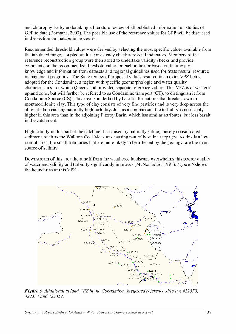
Sustainable Rivers Audit Pilot Audit – Water Processes Theme Technical Report
27
and chlorophyll-a by undertaking a literature review of all published information on studies of GPP to date (Bormans, 2003). The possible use of the reference values for GPP will be discussed in the section on metabolic processes. Recommended threshold values were derived by selecting the most specific values available from the tabulated range, coupled with a consistency check across all indicators. Members of the reference reconstruction group were then asked to undertake validity checks and provide comments on the recommended threshold value for each indicator based on their expert knowledge and information from datasets and regional guidelines used for State natural resource management programs. The State review of proposed values resulted in an extra VPZ being adopted for the Condamine, a region with specific geomorphologic and water quality characteristics, for which Queensland provided separate reference values. This VPZ is a ‘western’ upland zone, but will further be referred to as Condamine transport (CT), to distinguish it from Condamine Source (CS). This area is underlaid by basaltic formations that breaks down to montmorillonite clay. This type of clay consists of very fine particles and is very deep across the alluvial plain causing naturally high turbidity. Just as a comparison, the turbidity is noticeably higher in this area than in the adjoining Fitzroy Basin, which has similar attributes, but less basalt in the catchment. High salinity in this part of the catchment is caused by naturally saline, loosely consolidated sediment, such as the Walloon Coal Measures causing naturally saline seepages. As this is a low rainfall area, the small tributaries that are more likely to be affected by the geology, are the main source of salinity. Downstream of this area the runoff from the weathered landscape overwhelms this poorer quality of water and salinity and turbidity significantly improves (McNeil et al., 1991). Figure 6 shows the boundaries of this VPZ.
Figure 6. Additional upland VPZ in the Condamine. Suggested reference sites are 422350, 422334 and 422352.

Sustainable Rivers Audit Pilot Audit – Water Processes Theme Technical Report
28
This iterative process of setting reference condition resulted in a fairly broad set of reference values where observations were also pooled across seasons. The members of the reference reconstruction group acknowledged that these values were better defined than the values listed in the NWQMS, however they expressed relatively low confidence in the accuracy and usefulness of the reference condition given the large variability associated with many indicators. No power analysis was undertaken on the values derived for reference, in part because the iterative process has included expert opinion and revisions of State water quality datasets. However, the power analysis that was undertaken on the data for the Pilot study will give some indication on how many observations would be required (from best available sites) to set a reference condition with a quantifiable confidence limit. The list of reference condition values (upper and lower boundaries) is given in Table 9.
Table 9. Reference values (upper [H] and lower bounds [L]3) for VPZ’s in each of the four Pilot valleys as defined by the reference reconstruction group. CS = Condamine source, CT = Condamine transport (central), CD = Condamine deposition, LS = Lachlan source, LD = Lachlan deposition, OS = Ovens source, OD = Ovens deposition, MD = Murray deposition (below Darling confluence). Values between upper and lower bound are considered equal to reference (non-impacted).
VP
Z
limit
Turb
idity
(N
TU)
Tem
pera
ture
(˚C
)
pH
Con
duct
ivity
(µ
S/c
m)
TN (m
g/L)
TKN
(mg/
L)
Nox
(mg/
L)
TP (m
g/L)
DO
(%sa
t)
GP
P (m
g C
/m2/
day)
**
R24
(mg
C/m
2/da
y)**
CH
LA (µ
g/L)
GP
P/R
24
ratio
CS L 5 14 7 150* 0.46 0.45 0.01 0.04 88.5 - - 0 0.3
H 20 24 8.3 300* 1.4 1.11 0.29 0.07 103 200 500 5 3
CT L 10 14 7 800* 1.04 0.93 0.11 0.06 51.4 - - 3 0.3
H 150 24 8.4 1800* 7.3 6.99 0.31 1 132 - - 10 3
CD L 100* 15 7.0 100 0.75 0.74 0.01 0.13 44.4 - - 3 0.3
H 800* 26 8.0 230 1.5 1.14 0.36 0.55 95.7 500 800 10 3
LS L 2 8.5 7.1 200 0.25 0.249 0.001 0.008 85 - - 1 0.3
H 10 23 8.3 500 0.5 0.48 0.02 0.017 105 200 500 3 3
LD L 15 10 7.1 300 0.45 0.449 0.001 0.023 85 - - 2 0.3
H 30 25 8.3 600 0.6 0.58 0.02 0.039 105 500 800 5 3
OS L 0 8.6 6.5 10 0.15 0.13 0.02 0.01 90 - - 0 0.3
H 2 12.5 7.1 55 0.35 0.25 0.1 0.025 110 200 500 3 3
OD L 0 9.84 6.7 42 0.3 0.22 0.08 0.01 85 - - 0 0.3
H 10 20.8 7.4 100 0.6 0.45 0.15 0.045 105 500 800 5 3
MD L 0 12 7.5 0 0 0 0 0 80 - - 0 0.3
H 76 28 8 400 1.02 1 0.02 0.06 110 500 800 10 3
* These values were based on 20th and 80th percentiles calculated from MRHI sites; different datasets appear to provide a wide range of percentile values; the reference values listed here are provisory and would need expert revision. For conductivity, cumulative values would indicate that Condamine depositional would have highest values, something contradicted by these reference values. Groundwater influxes, lack of connectivity are possible mechanisms explaining this anomaly. ** No reference values were provided by the States for this indicator, instead reference values resulting from the literature review were used (Bormans, 2003).
3 The reference values refer to ‘natural’, and should be distinguished from targets.
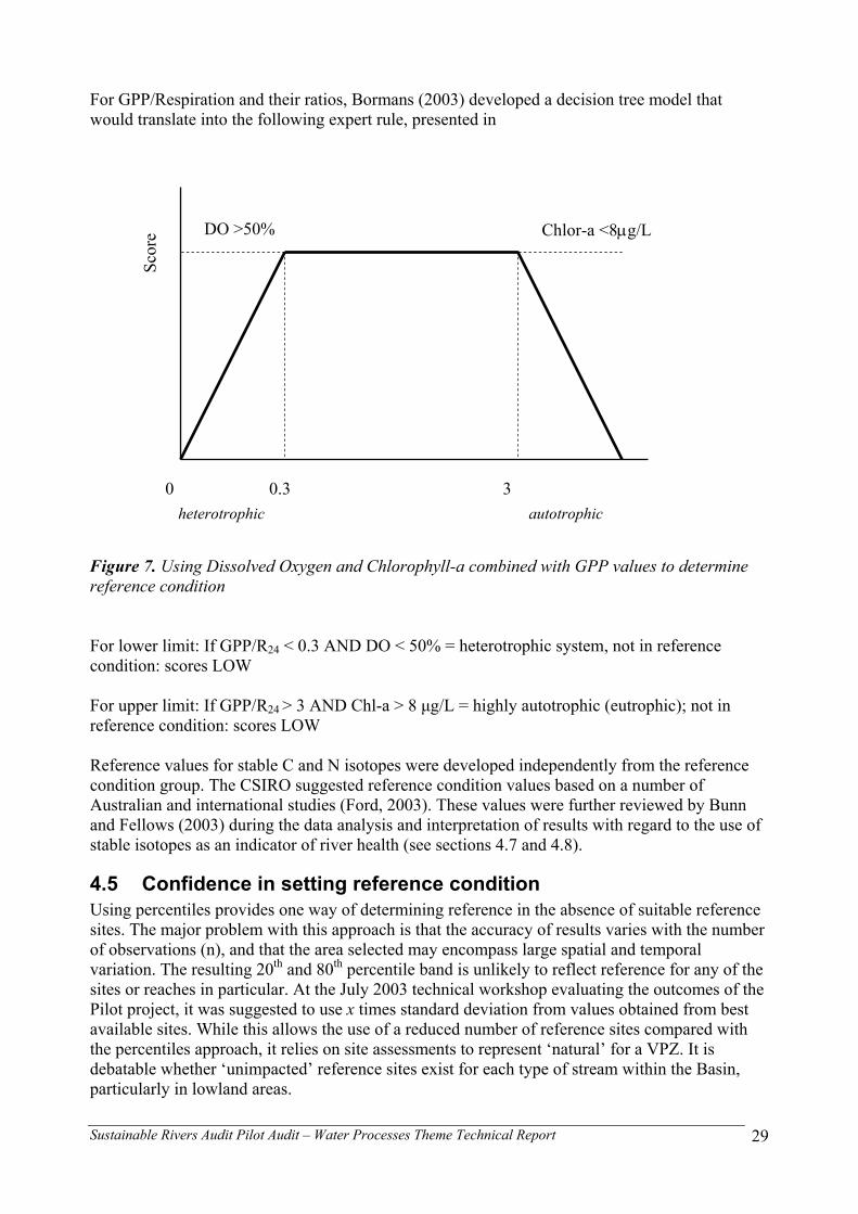
Sustainable Rivers Audit Pilot Audit – Water Processes Theme Technical Report
29
For GPP/Respiration and their ratios, Bormans (2003) developed a decision tree model that would translate into the following expert rule, presented in
Figure 7. Using Dissolved Oxygen and Chlorophyll-a combined with GPP values to determine reference condition
For lower limit: If GPP/R24 < 0.3 AND DO < 50% = heterotrophic system, not in reference condition: scores LOW
For upper limit: If GPP/R24 > 3 AND Chl-a > 8 µg/L = highly autotrophic (eutrophic); not in reference condition: scores LOW Reference values for stable C and N isotopes were developed independently from the reference condition group. The CSIRO suggested reference condition values based on a number of Australian and international studies (Ford, 2003). These values were further reviewed by Bunn and Fellows (2003) during the data analysis and interpretation of results with regard to the use of stable isotopes as an indicator of river health (see sections 4.7 and 4.8).
4.5 Confidence in setting reference condition Using percentiles provides one way of determining reference in the absence of suitable reference sites. The major problem with this approach is that the accuracy of results varies with the number of observations (n), and that the area selected may encompass large spatial and temporal variation. The resulting 20th and 80th percentile band is unlikely to reflect reference for any of the sites or reaches in particular. At the July 2003 technical workshop evaluating the outcomes of the Pilot project, it was suggested to use x times standard deviation from values obtained from best available sites. While this allows the use of a reduced number of reference sites compared with the percentiles approach, it relies on site assessments to represent ‘natural’ for a VPZ. It is debatable whether ‘unimpacted’ reference sites exist for each type of stream within the Basin, particularly in lowland areas.
Chlor-a <8µg/L DO >50%
0 3 0.3 autotrophic heterotrophic
Scor
e

Sustainable Rivers Audit Pilot Audit – Water Processes Theme Technical Report
30
Further work would certainly be required to better define reference condition taking into account:
• the selection of best available sites and criteria used
• temporal variation in reference conditions, associated with seasonal cycles
• possible spatial stratification based on geomorphology (it will be difficult to establish gradients of variability whilst discounting disturbance related to land use, etc).
Limited studies have been undertaken to develop an Observed/Expected model analogous to the AUSRIVAS model for macroinvertebrates (McNeil et al., 2000). Whilst this approach has some potential, the amount of work required may be substantial to cover the entire Basin, and requires substantial datasets which can only be built up over time. At the workshop the comment was also made that too much focus on reference condition was probably not very informative and trend detection over time was of higher importance, particularly once targets have been set. However, the approach of comparing against reference condition would allow a relative comparison of valley zones within the Basin on departure from reference, thus informing on the degree of departure from natural of modification of the river system compared to other valleys. Without a proper reference, trend detection may not be sufficient to set targets and improve river health. At the workshop, the observation was made that reference condition cannot be set for every event; it is important to look at reference for base-flow conditions. There was discussion about whether this missed the key ‘events’, but the point was made that it is not feasible to set up an events based sampling program for the entire Basin. Measuring water quality at base-flow conditions should indicate the capacity (resilience) of the system to recover from flood related events. Another shortcoming of the current approach that was identified is the possible lack of consistency between Pilot valleys in setting reference condition. For developing reference condition for all valleys in the Basin, a coordinated approach would be required which applies consistency checks for reference condition for each of the metrics from headwaters to lowland rivers across the Basin.
4.6 Departure from reference Two approaches for analysing the data and defining departure from reference were suggested for the SRA: 1) Treat sampling sites as replicates of the VPZ and carry out a power analysis to determine number of sites required to detect a 0.1, 0.2, 0.3 or 0.4 level of change with power of 0.8 and significance level of 0.1. The level of change would be used in a scaling system to define departure from reference. This would need to be done for each indicator separately, and expert rules would be needed to combine scores into an overall index for river health water (SR-WI). 2) Compliance monitoring. Treat each sampling site as an observation, and report the percentage of sites exceeding reference condition. If presented on a map, this will also give a location of site condition. A power analysis revealed that compliance type monitoring would require a lot more sites to be truly informative of a VPZ condition, which becomes problematic in terms of sampling frequency and trend detection (section 7.3).
4.7 Defining reference condition for stable nitrogen isotopes The reference condition for stable isotope ratios was undertaken by Ford (2003) and further reviewed by Bunn and Fellows (2003). Reference condition was determined by examining various studies previously undertaken. The CSIRO review suggested that nitrogen ratios of <-3‰ could be interpreted as fertilizer impacted and hence be indicative of anthropogenic changes in land use in upstream sections of the catchment relative to the sampling site. Values of > 6‰
Sustainable Rivers Audit Pilot Audit – Water Processes Theme Technical Report
31
would indicate human or animal contamination or extensive denitrification of fertilizer inputs. Non-impacted sites would be characterized by values ranging between -3‰ and +3‰. However, Bunn and Fellows observed that N-fixing blue green algae can also have values as low as -3‰, as well as submerged aquatic macrophytes in unimpacted systems (Boon & Bunn, 1994; Bunn et al. 1999). They suggest that only the upper reference limit of 6‰ would be used as an indication of anthropogenic inputs of N (manure or septic sewage sources). This reference condition has been used to interpret the results from the Pilot study, and to group data into the following categories:
Non-impacted: < 6‰
Impacted: 6-10‰
Severely impacted: > 10‰
4.8 Defining reference condition for Stable carbon isotopes Defining reference conditions for stable C isotopes was much more difficult, as the carbon content in dissolved CO2 may have been derived from different sources, depending on depth of the water column, stream flow, light as a limiting factor, groundwater influx etc. The CSIRO review concluded that for these reasons it is unlikely that the carbon isotope ratio will provide additional information to that which accrues from other measurements of metabolic activity and habitat characteristics (Ford, 2003).
Bunn and Fellows found that about 50% of C carbon isotope ratio variation could be explained by the level of gross primary production, which is why it has been proposed to use this indicator as a surrogate measure of GPP. There are however marked natural differences between some systems which would require setting reference values that are biome specific. Therefore, Bunn and Fellows recommended to use δ13C values as a check for GPP measures at the extreme end of the observed ranges rather than using it as a surrogate measure per se, using the following guidelines:
If δ13C <-35‰ then GPP ≈ <0.1 g C m-2 day-1 (= very low productivity)
If δ13C> -25‰ then GPP ≈ > 1 g C m-2 day-1 (= high productivity)
Note that metabolic processes are usually defined as the ratio of GPP over R to determine if a system is in balance. By estimating GPP values alone from carbon isotopes little insights can be gained on the condition of in-stream metabolic processes.

Sustainable Rivers Audit Pilot Audit – Water Processes Theme Technical Report
32
5 Metabolic process indicators
5.1 Methods Metabolic process indicator methods have been developed for research purposes, and at the workshop it was decided that the Pilot project should investigate to what extent these methods are suitable for routine monitoring purposes. The use of benthic domes and the required expertise necessitated a small scale trial. The DEC , which has the required expertise and equipment to carry out such experiments, volunteered to undertake this project and it was decided to limit this trial to the Lachlan Pilot valley only. The results and recommendations from this project are documented in ‘Water Column and Benthic Metabolism: Review of Concepts and Methods for Monitoring for the Murray Darling Sustainable Rivers Audit (MDBSRA)’ (Poirier et al., 2003). Relevant sections of the report and a summary of the results and recommendations are presented in section 5.2. Three methods for measuring metabolism rates were trialled: whole-stream metabolism, benthic chambers and pelagic chambers, and their use and compatibility as monitoring tools were discussed on the basis of the experiments, technical problems and results obtained. There are advantages and limitations for each of the methods. In short, the chamber methods are only measuring parts of the metabolic processes taking place in the water column, and therefore direct comparisons between data collected with the chambers and the whole-stream method are not possible. The whole-stream method provides a more integrated measure of metabolic processes, but the exchange rate of oxygen between the atmosphere and the water surface can only be estimated. In contrast exchange rates of oxygen between the atmosphere and the water column can be measured fairly accurately in enclosed chambers. On the other hand there are possible distortions of the metabolic processes due to light fractionation and reduction within the chambers, so that rates do not necessarily reflect what is happening in the surrounding water column. The enclosure also means that only benthic or pelagic components of the metabolic process are quantified. Comparisons between chambers and whole-stream methods reveal that chambers consistently underestimate metabolic rates, but the proportion of underestimation can vary considerably (Poirier et al., 2003).
5.1.1 Whole-stream metabolism Ten sites were selected in the Lachlan Valley, where data loggers were deployed to measure dissolved oxygen (DO) consumption, temperature and pH in winter (August 2002) and summer (February 2003) for a 24hr period (diurnal cycle). Four of those sites were located in the source valley process zone where benthic chambers were deployed; six sites were situated in the depositional valley process zone where pelagic chambers were deployed to trial the other two methods. All three methods measure production/respiration ratios; the whole-stream method in an integrated fashion whereas benthic or pelagic methods only measure ratios for the respective parts of the water column encapsulated by the chambers. For the whole-stream method cosine corrected light (PAR) measurements were also recorded, and whole-stream metabolism parameters were calculated as per detailed method description in Poirier et al. (2003). In addition, diurnal DO data were collected at a number of sites in Victoria and Queensland with dataloggers using the same method (APPENDIX 3), but unfortunately PAR measurements were not recorded and light conditions had to be inferred from meteorological datasets. Data from 8 and 2 sites respectively were included in the analysis.

Sustainable Rivers Audit Pilot Audit – Water Processes Theme Technical Report
33
5.1.2 Benthic Chambers Benthic chambers were deployed in the Lachlan Source VPZ at four sites, where streams are shallow (typically <0.5 m deep) and cobble substrate is available. A full description of the benthic chambers is provided in Poirier et al. (2003). The production/respiration rates of biofilm attached to a cobble are measured and this requires placing the chamber on the substrate, then placing a cobble inside the chamber without disturbing the attached biofilm. Water was then recirculated through the chamber and DO and temperature readings were logged every 10 minutes for a 24 hr period.
5.1.3 Pelagic Chambers Pelagic chambers are transparent spheres that are suspended in the euphotic zone of the water column, typically in the deeper and slower flowing sections of the river. In the Lachlan, pelagic chambers were deployed at six sites in the lowland sections of the valley. As for benthic chambers, water is circulated to prevent settling of suspended particles and phytoplankton and DO and temperature readings were logged every 10 minutes for a 24 hr period.
5.2 Results and discussion
5.2.1 Whole-stream metabolism The DEC compiled all results for the diurnal dissolved oxygen data collected by other States for the Pilot project. No data were available for the Lower Murray, and only two valid observations were included for the Condamine and eight for the Ovens. Many of the light intensity data had to be inferred as the datasets obtained from other states were incomplete. A software model developed by Mike Grace from Monash University (Grace and Harper, 2003) was used to back out various factors associated with the model of oxygen concentration in stream water, and only the data with best fit were included for possible analysis. To do this, a subjective scoring system (1-4) was developed and only observations rated 1-2 were included as data within the experience of the model. Examples of the scoring are presented in Figure 8 to Figure 12 below.
Lach230A - Summer
9.69.810
10.210.410.610.8
1111.211.411.6
13:20
14:50
16:20
17:50
19:20
20:50
22:20
23:50 1:2
02:5
04:2
05:5
07:2
08:5
010:2
011
:50
Time of Day
DO
(mg/
L)
MeasuredCalculated
Figure 8. Rating 1 Good fit with measured data. Re-aeration coefficient K=1.93E-5

Sustainable Rivers Audit Pilot Audit – Water Processes Theme Technical Report
34
Lach230A - Winter
0
2
4
6
8
10
1217
:00
18:2
0
19:4
0
21:0
0
22:2
0
23:4
0
1:00
2:20
3:40
5:00
6:20
7:40
9:00
10:2
0
11:4
0
13:0
0
14:2
0
15:4
0
Time of Day
DO
(mg/
L)
MeasuredCalculated
Figure 9. Rating 1 Good fit but with very small re-aeration coefficient K= 2.92E-198
Lach245B
55.5
66.5
77.5
88.5
9
16:40
18:10
19:40
21:10
22:40
0:10 1:40 3:10
4:40
6:10 7:40
9:10
10:40
12:10
13:40
15:10
16:40
Time of Day
DO
(mg/
L)
MeasuredCalculated
Figure 10. Rating 2 Satisfactory fit. K=6.05E-195
4224008_2
123456789
16:0
4
18:0
4
20:0
4
22:0
4
0:04
2:04
4:04
6:04
8:04
10:0
4
12:0
4
14:0
4
16:0
4
18:0
4
20:0
4
22:0
4
0:04
2:04
4:04
Time of Day
DO
(mg/
L)
MeasuredCalculated
Figure 11. Rating 3 Poor fit – data outside the experience of the model. K=1.66E-11

Sustainable Rivers Audit Pilot Audit – Water Processes Theme Technical Report
35
CDL Spring
9.69.810
10.210.410.610.8
1111.2
16:00
17:30
19:00
20:30
22:00
23:30
1:00
2:30
4:00
5:30 7:00 8:30
10:00
11:30
13:00
14:30
Time of Day
DO
(mg/
L)
MeasuredCalculated
Figure 12. Rating 4 Poor fit – data outside the experience of the model. K=1.60E-4
Another indication of some fundamental problems with the procedure is the modelled results for the re-aeration coefficient, where values would be expected to range between ~ 1*E-4 mg.L-1.s-1 (high rate) and ~ 1*E-6 mg.L-1.s-1 (low rate). About 66% of the data returned re-aeration coefficients of <1*E-6 mg.L-1.s-1 (too low). This would indicate that the other outputs (respiration and production) are perhaps not credible. A possible number of factors could be responsible including:
• absence of accurate specific light data (light was not logged in the Ovens and in the Condamine, and there were gaps in the data for the Lachlan)
• poorly measured data
• real but anomalous data (different water mass moving through the system, changing stratification in the stream, etc)
• inadequacies in the interpretive process
• limitations of the model
The anomalies in the Pilot data have not been resolved and these and other factors would need further investigation as part of a method development for whole-stream methods of GPP measurement. This preliminary assessment reveals that the technique can work but the limitations will need to be better delineated. In absence of a fully developed whole-stream method diurnal dissolved oxygen could be used as a substitute indicator. The results with accepted ratings (including low re-aeration coefficients) are presented in Table 10 below. The column of interest is the P/R ratios. Compared to reference values listed in Table 9, none of the ratios exceeds 3, which indicated that all measurements are within the upper reference limit. There are four observations that have P/R ratios <0.3 (numbers in red font); of those three are from site Lach13 and one from an Ovens site. The dissolved oxygen values for those sites are all >50%, therefore none of these observations represents a departure from reference (Table 9).

Sustainable Rivers Audit Pilot Audit – Water Processes Theme Technical Report
36
Table 10. Results (averages from replicates) for all whole-stream metabolism methods (Condamine, Lachlan and Ovens) determined by diurnal Dissolved Oxygen methods (a=Solar radiation model - accurate coordinates; b=Solar radiation model - estimated coordinates; c=Generic set created from logged data; d=Generic set created from logged data - not yet adjusted to microeinsteins; e=Logged data - not yet adjusted to microeinsteins). P/R values in red indicate departure from ‘reference’(see Table 9). Ratings see Figures 8-12.
Site
cod
e
Num
ber
of
repl
icat
es
P/R
Dai
ly P
hoto
synt
h.
m
etho
d 1
(mg
O2/
L/da
y)
Dai
ly P
hoto
synt
h.
m
etho
d 2
(mg
O2/
L/da
y)
Com
mun
ity
Res
pira
tion
(mg
O2/
L/da
y)
DO
max
%
DO
min
%
DO
% r
ange
DO
max
con
c.
(mg/
L)
DO
min
con
c.
(mg/
L)
DO
con
c. R
ange
(m
g/L)
R R
espi
ratio
n (m
g/L/
s)
K R
e-ae
ratio
n co
effic
ient
(mg/
L/s)
Rat
ing
light
met
hod
CBH 1 0.12 1.82 1.79 14.45 83.8 65.7 18.08 7.85 6.36 1.49 1.67E-04 5.59E-05 1 a
CBJ 1 0.50 2.58 2.55 5.15 100.3 85.2 15.14 8.99 8.05 0.94 5.97E-05 3.76E-05 1 a
CBW 1 1.11 7.77 8.53 7.32 91.0 43.6 47.39 8.40 4.30 4.10 8.48E-05 0.0E+00 1 b
CBJ 1 0.41 2.35 2.32 5.64 96.4 78.5 17.96 8.37 6.94 1.43 6.53E-05 2.79E-05 1.5 a
CBV 1 0.57 1.32 1.38 2.38 90.8 74.9 15.89 7.60 6.40 1.20 2.76E-05 5.04E-06 2 b
CBV 1 0.81 2.10 2.08 2.59 58.4 31.8 26.62 4.87 2.70 2.17 2.99E-05 7.74E-11 2 b
CBA 1 0.96 2.07 2.04 2.14 98.8 82.2 16.67 8.50 7.50 1.00 2.48E-05 5.60E-11 2 b
CBG 1 0.98 1.65 1.65 1.68 88.3 74.3 14.01 9.13 8.41 0.72 1.94E-05 6.53E-11 2 a
4222074_2 1 1.10 4.91 4.84 4.41 140.9 96.4 44.48 10.00 7.56 2.44 5.11E-05 1.96E-11 2 a
4223081_2 1 0.96 10.63 11.04 11.26 84.1 31.0 53.10 6.69 2.62 4.07 1.30E-04 2.61E-11 2 a
Lach13 1 0.34 0.55 0.65 1.77 92.7 87.3 5.43 10.10 9.60 0.50 2.04E-05 9.02E-06 1 c
Lach13 2 0.28 0.49 0.52 1.83 90.9 85.6 5.31 9.90 9.40 0.50 2.11E-05 8.72E-06 1 c
Lach203 1 0.61 0.40 0.41 0.67 100.1 96.7 3.36 10.90 10.60 0.30 7.73E-06 1.31E-05 1 c
Lach204 1 1.08 1.97 2.26 1.96 107.9 93.4 14.44 13.00 11.90 1.10 2.27E-05 1.52E-05 1 c
Lach220 2 0.93 0.31 0.34 0.35 100.7 96.8 3.82 11.00 10.70 0.30 4.04E-06 1.35E-07 1 c
Lach230 1 0.74 1.69 2.06 2.54 104.2 89.7 14.44 11.30 10.30 1.00 2.94E-05 1.93E-05 1 c
Lach230 2 0.93 1.74 2.10 2.06 107.0 92.4 14.57 11.60 10.60 1.00 2.38E-05 1.95E-05 1 c
Lach244 1 0.95 1.54 1.73 1.71 111.1 100.4 10.61 12.40 11.60 0.80 1.98E-05 0.0E+00 1 c
Lach245 1 1.08 1.04 1.23 1.06 99.6 90.6 9.03 11.40 10.80 0.60 1.22E-05 7.5E-199 1 c
Lach204 1 1.17 7.38 7.30 6.29 97.3 43.0 54.30 7.80 3.90 3.90 7.28E-05 8.8E-200 1 e
Lach204 2 1.12 6.64 6.78 5.97 110.7 50.4 60.26 8.90 4.50 4.40 6.91E-05 5.1E-199 1 e
Lach230 1 1.14 8.92 10.67 8.60 126.5 65.0 61.48 9.90 5.50 4.40 9.96E-05 2.9E-198 1 d
Lach230 2 1.14 9.47 11.38 9.12 126.0 62.5 63.51 9.90 5.30 4.60 1.06E-04 3.3E-198 1 d
Lach244 1 1.18 5.40 6.08 4.86 101.8 67.3 34.55 7.90 5.60 2.30 5.62E-05 4.9E-197 1 e
Lach244 2 1.15 5.29 5.91 4.88 106.2 73.2 32.97 8.20 6.10 2.10 5.65E-05 4.9E-197 1 e
Lach203 2 0.44 0.44 0.45 1.01 99.1 95.8 3.26 10.70 10.50 0.20 1.16E-05 1.91E-05 1.5 c
Lach207 1 1.00 5.33 5.84 5.56 116.5 81.6 34.86 12.10 9.10 3.00 6.43E-05 5.38E-08 1.5 c
Lach220 1 0.52 0.18 0.19 0.36 100.1 96.9 3.16 10.90 10.70 0.20 4.18E-06 5.52E-06 1.5 c
Lach244 2 1.03 1.42 1.72 1.53 99.2 88.8 10.39 11.06 10.18 0.88 1.77E-05 2.6E-199 1.5 c
Lach242 1 1.00 8.77 9.28 9.00 119.6 55.1 64.52 9.50 4.80 4.70 1.04E-04 2.0E-196 1.5 e
Lach242 2 1.02 8.88 9.36 8.98 130.8 63.1 67.69 10.40 5.50 4.90 1.04E-04 3.2E-196 1.5 e
Lach13 1 0.05 0.52 0.52 10.02 68.7 61.2 7.48 5.50 5.00 0.50 1.16E-04 3.65E-05 2 d
Lach13 2 0.05 0.58 0.29 8.17 81.0 72.0 9.04 6.50 5.90 0.60 9.45E-05 4.22E-05 2 e
Lach207 1 0.97 17.31 18.60 18.46 126.2 14.6 111.66 10.10 1.20 8.90 2.14E-04 0.0E+00 2 d
Lach220 1 1.04 0.55 0.55 0.53 82.4 75.9 6.50 6.60 6.20 0.40 6.09E-06 2.5E-200 2 e
Lach245 1 0.82 6.58 4.12 6.54 112.4 62.7 49.65 9.00 5.40 3.60 7.57E-05 2.7E-195 2 e
Lach245 2 0.76 5.68 3.65 6.13 109.0 64.8 44.05 8.80 5.60 3.20 7.10E-05 6.1E-195 2 e

Sustainable Rivers Audit Pilot Audit – Water Processes Theme Technical Report
37
5.2.2 Whole-stream method power analysis A power analysis conducted on the data presented in Table 10 for the whole-stream method established that to detect a level of change of 0.1 with confidence α = 0.05 and power = 0.8, in the Ovens valley 13 sites would be required and in the Lachlan 10 sites. The mean and standard deviation for the Condamine did not allow establishing the number of sites required, and no data were available for SA.
5.2.3 Chambers The GPP and R24 values in the Lachlan are provided in Table 11. They were considerably lower than those reported in the DIBM3 study in the Condamine, Balonne and Narran Rivers (Smith and Storey, 2001). GPP and R24 were higher in summer and both measures tended to be highest in the Lower reaches of the Lachlan River (Figure 13 and Table 12 present results for summer only). This would suggest that the upland riverine model and the lowland riverine productivity concept may have some validity for the Lachlan, but considerably more data would be required to confirm this indication.
Table 11. Minimum and maximum values for pelagic and benthic chambers for Winter and Summer. Site and replicate numbers between brackets; Respiration rates are presented as negative numbers (consumption of oxygen).P/R values in red indicate departure from ‘reference’(see Table 9).
Pelagic Spheres Winter min Winter max Summer min Summer max
GPP (Mg O2/L/day) 0.69 (Lach13r1)
4.6 (Lach 230r2)
1.09 (Lach 13r1)
7.27 (Lach 207r2)
R24 (Mg O2/L/day) -0.37 (Lach 207r3)
-2.59 (Lach 230r2)
-0.33 (Lach 13r2)
-4 (Lach 230r1)
P/R ratios 1.4 (Lach 232r1)
5.32 (Lach 230r3)
1.14 (Lach 203r2)
5 (Lach 13r2)
Benthic Domes
GPP (Mg O2/L/day) 0.11 (Lach 204r2)
0.54 (Lach 242r3)
0.22 (Lach 204r3)
3.58 (Lach 242r2)
R24 (Mg O2/L/day) -0.08 (Lach 204r2)
-0.53 (Lach 242r3)
-0.27 (Lach 204r2)
-2.82 (Lach 242r3)
P/R ratios 0.51 (Lach 245r4)
2.13 (Lach 245r2)
0.75 (Lach 204r3)
2.07 (Lach 244r2)
Reference conditions for chamber methods have not been determined, but since the values underestimate total GPP and R, it is probably valid to assume that if upper limits set for whole-stream methods (>3 gC.m-2.day-1) are exceeded it is very likely that the site where condition is measured is eutrophic and not within reference, since reference condition for chamber measurements would be set lower than for the whole-stream method. Exceedence of reference for whole-stream (values listed in red font in Table 11) would need to be confirmed by measuring chlorophyll-a production on which currently data are not available. In the lower reaches of the Lachlan, it appears that reference condition is exceeded in both seasons, whereas in the upper Lachlan the ratios never reach the upper limit. This observation is however not confirmed by the results for whole-stream methods, and the power analysis (see section below) determines that many more measurements would be required to make any meaningful interpretations of the results. Lower limits of reference condition could not be inferred from whole-stream methods as
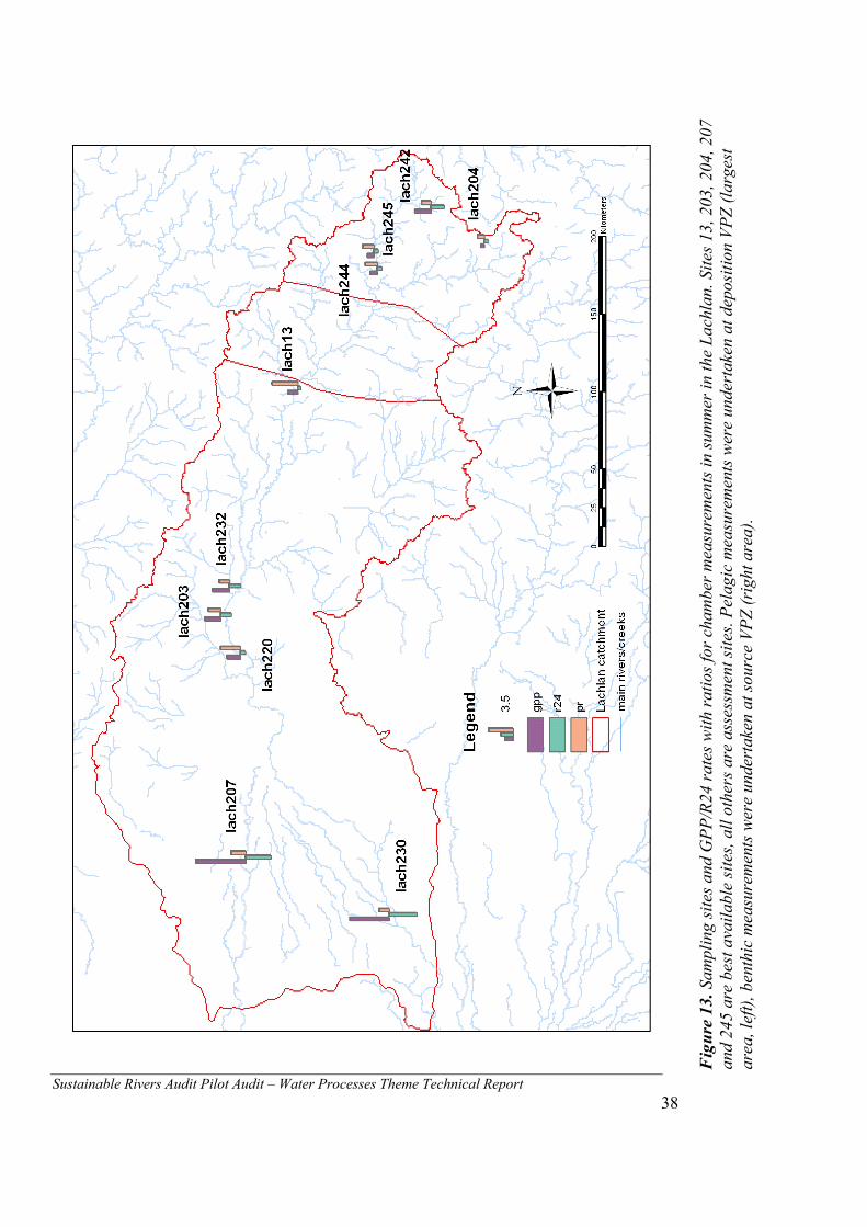
Sustainable Rivers Audit Pilot Audit – Water Processes Theme Technical Report 38
Fig
ure
13. S
ampl
ing
site
s and
GPP
/R24
rate
s with
ratio
s for
cha
mbe
r mea
sure
men
ts in
sum
mer
in th
e La
chla
n. S
ites 1
3, 2
03, 2
04, 2
07
and
245
are
best
ava
ilabl
e si
tes,
all o
ther
s are
ass
essm
ent s
ites.
Pela
gic
mea
sure
men
ts w
ere
unde
rtak
en a
t dep
ositi
on V
PZ (l
arge
st
area
, lef
t), b
enth
ic m
easu
rem
ents
wer
e un
dert
aken
at s
ourc
e VP
Z (r
ight
are
a).

Sustainable Rivers Audit Pilot Audit – Water Processes Theme Technical Report
39
Table 12. GPP and R24 rates and P:R ratios for chambers in the Lachlan valley in summer – values for Figure 13. (*denotes best available sites)
Site method VPZ GPP
(Mg O2/L/day)
R24
(Mg O2/L/day)
P/R ratio
Lach13* Pelagic spheres deposition 1.36 -0.42 3.58
Lach203* Pelagic spheres deposition 2.17 -1.47 1.71
Lach207* Pelagic spheres deposition 6.93 -3.47 2.01
Lach 220 Pelagic spheres deposition 1.87 -0.68 2.76
Lach230 Pelagic spheres deposition 5.48 -3.84 1.43
Lach 232 Pelagic spheres deposition 2.26 -1.66 1.40
Lach 204 Benthic domes source 0.46 -0.50 0.92
Lach 242 Benthic domes source 2.25 -1.82 1.28
Lach 244 Benthic domes source 1.00 -0.63 1.68
Lach 245* Benthic domes source 0.88 -0.55 1.59
the proportion of GPP not measured by chamber methods would need to be quantified. Site 230 appears to have high production and low respiration rates in winter, but the maximum P/R ratio associated with this site is from another replicate. In winter, site 230 appears to have the highest production and respiration rate for replicate 2, whereas at replicate 3 respiration is so much lower that the P/R ratio is highest. This suggests that even at the same site large variability is possible, an indication perhaps that pelagic measurements may not fully integrate metabolic processes in the entire water column. Replicate 2 from site 13 has the lowest respiration rate and the highest P/R ratio. For benthic domes, minimum values for both production and respiration are found at site 204 (replicate 2), whereas maximum values are found at site 242 (replicate 2). This contrast in the source VPZ suggests that the two models proposed (high OM input and low OM input) may have some validity, but the small dataset would require further investigation. Certainly, minimum values for site 204 are maintained over summer suggesting that this site is in a relatively undisturbed area characterised by shading riparian vegetation. Similarly, maximum values for site 242 appear to be maintained over summer, although by different replicates this time.
5.3 Power analysis A power analysis conducted on the data for both seasons for pelagic chambers and benthic domes revealed that to detect a level of change of 0.1 with confidence α = 0.05 and power = 0.8, there were 9 sites required for pelagic chambers. The mean and standard deviation for domes did not allow a power analysis, but if data for pelagic and benthic chambers were combined 10 sites were required. Combining both methods is however not suitable since different parts of the metabolic processes are measured; it is therefore anticipated that in both an upland and lowland VPZ ten sites would be required to detect a 10% change. The results cannot directly be compared between benthic and pelagic chambers, but given that reference condition can be developed for each method it would allow comparing upland VPZ’s across catchments with each other, as well as comparing lowland VPZ’s across catchments.

Sustainable Rivers Audit Pilot Audit – Water Processes Theme Technical Report
40
6 N & C stable isotope ratio indicators
6.1 Background Stable carbon and nitrogen isotope indicators have been trialled and adopted as part of the Ecosystem Health Monitoring Program in South East Queensland (Smith and Storey, 2001). The workshop at the beginning of the Pilot project recommended that these indicators should be further investigated (Table 5), and for the Sustainable Rivers Pilot Project, samples of algae and vascular plants were collected to assess the utility of stable carbon (δ13C) and nitrogen (δ15N) isotopes as indicators of river health. Stable nitrogen isotopes have been used as tracers of anthropogenic sources of nitrogen in aquatic ecosystems, while stable carbon isotopes have been used in identifying sources of organic carbon that support food webs. The CSIRO reviewed the potential of these indicators (Ford, 2003), and this review raised a number of questions to be answered from the trials:
1. Can δ13C values be used as a surrogate for GPP measurements?
2. What is the difference in using vascular plant samples versus attached algae? What is the time-scale and turnover rate? Accuracy/confidence of results?
3. Is the δ15N ratio a reliable indicator of land use (industrial fertilizers/sewage) and its losses to the river system(s)? Can it be used as a baseline as recommended in the CSIRO report?
4. What number of samples is required to make assessments of river condition at a particular scale (Valley Zones – upland and lowland), and to collect adequate baseline information?
The SRA project team subsequently identified the need for expert knowledge to assist in the interpretation of the laboratory analysis of the algal and vascular samples. The data analysis, interpretation and major recommendations regarding the utility of the indicators were investigated by Bunn and Fellows and are contained in the ‘Report on Stable Isotope Indicators’ (Bunn and Fellows, 2003).
6.2 Methods During the Pilot project, a number of samples of algal and vascular plant material were collected from the streambed at sites sampled for other water quality indicators within the Condamine, the Lachlan and the Ovens catchments (see section 7. Water Quality Indicators). The material was collected according to the protocols developed for the Pilot project (APPENDIX 3). The samples were collected during spring 2002 and summer 2003, and were labelled and stored frozen for further analysis. Quality control of the sampled material resulted in samples being submitted for analysis being restricted to algal and vascular samples from the Lachlan and Ovens rivers only, as given in Table 13:
Table 13. Number of samples analysed for δ13C and δ15N for the Pilot SRA NSW VIC Algae Vascular Algae Vascular Spring 2002 22 16 5 3 Summer 2003 24 29 21 12 Total 46 45 26 15
Samples were analysed by mass spectrometry for stable C and N isotope ratios at Griffith University, and the results of data analysis and interpretation was presented in Bunn and Fellows (2003), including a comparison against reference condition derived from other studies for these indicators.

Sustainable Rivers Audit Pilot Audit – Water Processes Theme Technical Report
41
6.3 Results The result of the N and C Stable Isotope ratios is given in Table 14 and Table 15 below.
Table 14: Elemental % composition and isotope ratios (isotopic delta) for C and N in ‰ for each of the samples for algal plant material.
Sample Details Elemental Isotopic Index Site Season Algal or Vasc. % Composition Delta (‰)
(C) (N)
(C13)* 0.1-1gC <0.1gC >1gC
(N15)* No impact
Impact Severe impact
1 LACH06 Spring 2002 A 12.7 1.2 -29.4 11.0 2 LACH201 Spring 2002 A 36.2 1.7 -26.9 5.0 3 LACH202 Spring 2002 A 36.2 2.2 -21.9 6.9 4 LACH205 Spring 2002 A 19.5 2.7 -35.9 6.6 5 LACH206 Spring 2002 A 13.7 0.9 -32.3 2.1 6 LACH207 Spring 2002 A 12.7 0.8 -26.9 2.8 7 LACH223 Spring 2002 A 18.6 2.0 -18.1 0.0 8 LACH227 Spring 2002 A 35.5 3.0 -17.1 -0.1 9 LACH230 Spring 2002 A 27.2 3.4 -18.7 -6.2
10 LACH238 Spring 2002 A 23.5 1.7 -29.9 0.1 11 LACH240 Spring 2002 A 37.0 2.9 -20.6 4.2 12 LACH242 Spring 2002 A 34.6 1.4 -30.9 6.3 13 LACH244 Spring 2002 A 36.4 3.8 -28.0 6.2 14 LACH246 Spring 2002 A 37.8 1.8 -25.0 5.8 15 LACH247 Spring 2002 A 33.6 1.5 -36.7 5.5 16 LACH248 Spring 2002 A 32.3 2.7 -40.0 1.6 17 LACH249 Spring 2002 A 23.7 2.1 -41.0 6.2 18 LACH253 Spring 2002 A 33.0 2.2 -27.3 4.1 19 LACH254 Spring 2002 A 29.9 2.9 -36.5 7.0 20 LACH903 Spring 2002 A 36.0 2.7 -27.6 5.6 21 LACH06 Summer 2003 A 30.8 2.7 -34.5 11.4 22 LACH06 Summer 2003 A 39.0 1.8 -28.4 13.3 23 LACH106 Summer 2003 A 17.2 1.2 -30.0 3.9 24 LACH202 Summer 2003 A 27.2 1.8 -24.3 5.5 25 LACH203 Summer 2003 A 30.4 2.0 -30.0 8.8 26 LACH222 Summer 2003 A 28.3 1.1 -33.0 5.027 LACH223 Summer 2003 A 20.5 1.1 -22.2 2.4 28 LACH227 Summer 2003 A 31.8 1.2 -19.2 3.7 29 LACH232 Summer 2003 A 29.0 1.9 -28.4 7.5 30 LACH238 Summer 2003 A 29.8 1.2 -31.7 2.3 31 LACH240 Summer 2003 A 23.4 3.7 -25.2 5.2 32 LACH241 Summer 2003 A 28.0 2.1 -31.0 6.4 33 LACH242 Summer 2003 A 35.7 2.8 -11.3 3.5 34 LACH244 Summer 2003 A 34.7 1.8 -20.8 5.5 35 LACH254 Summer 2003 A 28.5 2.7 -36.0 8.2 36 LACH903 Summer 2003 A 31.2 0.9 -26.1 4.7 37 CBA Summer 2003 A 7.8 1.2 -30.6 9.1 38 CBK Spring 2002 A 39.7 4.4 -23.7 -0.2 39 CBW Spring 2003 A 7.6 1.0 -28.2 7.6 40 CDF Spring 2004 A 29.7 1.0 -28.2 4.5 41 CDI Spring 2005 A 13.1 1.2 -25.2 6.5 42 CDJ Summer 2003 A 31.4 2.4 -30.0 0.2 43 CDP Summer 2003 A 31.3 3.4 -31.7 6.7 44 CDU Spring 2002 A 33.5 2.5 -26.3 -1.1
Min. -41.0 -6.2 Max. -11.3 13.3 Mean -27.9 4.8 stdev 6.2 3.6 n 44 44 stdev / sqrt (n) 0.9 0.5
* see sections 4.7 and 4.8 (Defining reference condition for stable nitrogen and carbon isotopes) for legend explanation

Sustainable Rivers Audit Pilot Audit – Water Processes Theme Technical Report
42
Table 15. Elemental % composition and isotope ratios (isotopic delta) for C and N in ‰ for each of the samples for vascular plant material
Sample Details Elemental Isotopic Index Site Season Algal or % Comp Delta (‰)
Vasc. (C) (N)
(C13)* 0.1-1gC <0.1gC >1gC
(N15)* No impact
Impact Severe impact
1 LACH106 Spring 2002 V 18.5 0.5 -22.6 4.7 2 LACH201 Spring 2002 V 33.5 1.5 -27.0 7.2 3 LACH201 Spring 2002 V 29.8 2.6 -32.7 4.9 4 LACH201 Spring 2002 V 36.0 3.0 -28.5 0.8 5 LACH204 Spring 2002 V 30.2 2.0 -30.8 2.7 6 LACH204 Spring 2002 V 38.7 1.6 -22.3 4.0 7 LACH206 Spring 2002 V 37.3 2.5 -30.8 -0.1 8 LACH206 Spring 2002 V 23.4 1.8 -31.2 2.9 9 LACH206 Spring 2002 V 20.5 1.2 -33.8 5.4
10 LACH206 Spring 2002 V 27.3 2.1 -29.9 3.7 11 LACH207 Spring 2002 V 30.2 1.2 -23.1 6.2 12 LACH207 Spring 2002 V 17.7 1.1 -24.6 2.9 13 LACH207 Spring 2002 V 31.7 1.3 -20.3 5.4 14 LACH207 Spring 2002 V 23.8 1.3 -22.4 5.4 15 LACH237 Spring 2002 V 35.6 2.9 -22.9 7.2 16 LACH237 Spring 2002 V 32.5 1.6 -19.1 6.2 17 LACH238 Spring 2002 V 30.8 1.3 -29.2 6.9 18 LACH239 Spring 2002 V 33.6 3.6 -39.4 7.6 19 LACH240 Spring 2002 V 19.0 1.8 -32.9 5.6 20 LACH240 Spring 2002 V 31.4 2.1 -23.3 6.4 21 LACH241 Spring 2002 V 31.8 2.1 -30.3 3.9 22 LACH241 Spring 2002 V 34.5 2.2 -29.4 4.3 23 LACH242 Spring 2002 V 37.5 2.7 -23.1 6.5 24 LACH242 Spring 2002 V 33.1 2.2 -30.8 8.7 25 LACH242 Spring 2002 V 25.6 1.4 -26.4 8.7 26 LACH245 Spring 2002 V 33.0 1.1 -28.4 3.3 27 LACH06 Summer 2003 V 24.9 1.5 -26.7 10.0 28 LACH06 Summer 2003 V 15.7 1.3 -26.2 8.8 29 LACH106 Summer 2003 V 34.6 1.1 -24.7 3.2 30 LACH204 Summer 2003 V 38.5 1.7 -27.1 2.3 31 LACH204 Summer 2003 V 30.2 1.8 -28.4 2.8 32 LACH206 Summer 2003 V 31.0 2.1 -23.1 5.2 33 LACH206 Summer 2003 V 36.8 3.4 -30.5 0.5 34 LACH206 Summer 2003 V 25.1 2.0 -32.7 5.1 35 LACH206 Summer 2003 V 35.8 1.3 -28.6 7.6 36 LACH207 Summer 2003 V 37.3 2.8 -30.3 -0.5 37 LACH207 Summer 2003 V 31.7 2.1 -21.3 5.7 38 LACH207 Summer 2003 V 36.4 1.8 -30.0 8.5 39 LACH207 Summer 2003 V 26.9 1.7 -19.7 5.7 40 LACH223 Summer 2003 V 36.2 2.7 -30.2 8.0 41 LACH223 Summer 2003 V 30.2 1.0 -30.7 5.4 42 LACH237 Summer 2003 V 36.1 3.7 -29.4 -0.3 43 LACH237 Summer 2003 V 36.6 2.2 -28.9 7.6 44 LACH237 Summer 2003 V 31.3 1.8 -22.2 5.9 46 LACH238 Summer 2003 V 33.5 2.0 -29.5 3.6 47 LACH238 Summer 2003 V 35.2 1.0 -29.9 5.6 48 LACH238 Summer 2003 V 38.9 1.3 -12.9 5.2 49 LACH238 Summer 2003 V 35.2 1.8 -29.1 6.4 50 LACH239 Summer 2003 V 26.6 3.1 -41.4 4.7 51 LACH241 Summer 2003 V 24.3 2.1 -27.7 8.6 52 LACH242 Summer 2003 V 27.5 1.8 -26.0 3.8 53 LACH242 Summer 2003 V 23.3 1.7 -31.7 7.3

Sustainable Rivers Audit Pilot Audit – Water Processes Theme Technical Report
43
(Table 15 continued) Sample Details Elemental Isotopic Index Site Season Algal or % Comp Delta (‰)
Vasc. (C) (N)
(C13)* 0.1-1gC <0.1gC >1gC
(N15)* No impact
Impact Severe impact
54 LACH242 Summer 2003 V 38.1 2.7 -26.0 8.7 55 LACH245 Summer 2003 V 23.7 0.8 -22.1 0.9 58 CBG Spring 2002 V 31.4 2.5 -31.1 4.8 62 CBL Spring 2002 V 37.4 2.3 -27.7 -0.4 85 CDW Spring 2002 V 30.7 1.8 -29.6 3.3 71 CDJ Spring 2002 V 26.8 1.2 -30.9 1.2 72 CDK Spring 2002 V 27.8 2.2 -29.2 1.2 74 CDL Spring 2002 V 30.9 1.2 -22.7 0.1 76 CDM Spring 2002 V 20.5 0.9 -29.3 1.3 78 CDN Spring 2002 V 36.4 3.0 -29.3 -0.5 83 CDV Spring 2002 V 31.1 1.6 -29.4 1.0 57 CBA Spring 2002 V 39.9 2.3 -29.5 3.9 60 CBH Spring 2002 V 35.0 2.5 -32.9 4.8 65 CCY Spring 2002 V 30.9 2.1 -27.3 9.6 80 CDO Spring 2002 V 34.2 3.3 -28.6 5.3 81 CDP Spring 2002 V 38.3 2.3 -28.5 2.6 82 CDS Spring 2002 V 36.7 1.2 -19.4 5.2 66 CDA Spring 2002 V 32.0 4.0 -30.2 6.4 67 CDE Spring 2002 V 23.0 1.8 -29.8 9.9 77 CDM Summer 2003 V 24.2 1.7 -32.4 3.2 79 CDN Summer 2003 V 22.9 1.6 -30.7 0.4 63 CBL Summer 2003 V 37.7 3.1 -29.8 1.8 73 CDK Summer 2003 V 25.7 2.5 -30.7 4.5 86 CDW Summer 2003 V 21.0 2.2 -32.3 3.7 87 CEB Summer 2003 V 35.5 2.2 -29.7 3.0 59 CBG Summer 2003 V 27.3 1.7 -32.1 3.7 69 CDG Summer 2003 V 34.5 3.4 -30.2 5.0 75 CDL Summer 2003 V 20.5 1.4 -30.0 0.3 84 CDV Summer 2003 V 11.1 1.0 -31.1 1.6 64 CBV Summer 2003 V 36.7 1.6 -13.1 8.4
Min. -41.4 -0.5 Max. -12.9 10.0 Mean -27.9 4.6 stdev 4.7 2.8 n 82 82 stdev / sqrt (n) 0.5 0.3
* see sections 4.7 and 4.8 (Defining reference condition for stable nitrogen and carbon isotopes) for legend explanation
These data indicate that ‘considerable variation in stable nitrogen (and carbon) isotope signatures was found among samples of aquatic plants river sites in NSW and Victoria, collected in the SRA Pilot. δ15N values for the Lachlan ranged from –6.2 to 13.3 ‰ and those for the Ovens ranged from –1.1 to 12.2 ‰. The high level of variation in isotope values recorded among ‘replicate’ samples within sites/times is associated with a broad range in %N (and C) values. This, together with the noted variety of plant samples processed in the laboratory suggests that a single sample of a wide range of material was collected, including filamentous algae, N-fixing biofilms and emergent C4 macrophytes. The lack of detailed description of samples makes it very difficult to identify potential causes of this high within-site variability.’(Bunn and Fellows, 2003).

Sustainable Rivers Audit Pilot Audit – Water Processes Theme Technical Report
44
6.4 Discussion
6.4.1 Assessing stable nitrogen isotope data against reference condition Nitrogen fluctuations in the nitrogen cycle are typically large, and the variability in standard errors about the mean of between 10-15% found at replicate samples taken at various locations around Australia reflects this. Marked differences can be found between species (Boon and Bunn, 1994), and submerged macrophytes reveal a greater within site and temporal variation than is the case for filamentous algae. Despite this variability, values rarely exceed 6‰ (Bunn and Fellows, 2003) Bunn and Fellows (2003) state that several studies demonstrate a strong positive relationship between stable nitrogen isotope signatures of aquatic plants (or their consumers) and the degree of agricultural activity in catchments upstream. Three studies were listed in support of this relationship: Cabana (unpublished) r2 = 0.50; p <0.001, Hebert &Wassenaar (2002) r2 = 0.41; p<0.01 and Udy &Bunn (2001) r2 = 0.79; p = 0.018. Variables such as soil retention rates, geomorphology, climate, catchment size and type of agricultural land use, fertilizer rate application, frequency and timing are all possible factors confounding these results and accounting for the large range in correlation factors. In the course of the Pilot project it was not possible to provide Bunn and Fellows with catchment land use data, so this relationship could not be examined with data obtained from the Pilot study. Instead, the data were assessed against the reference condition described above. This assessment is discussed in the light of method development rather than focusing on the departure from reference. Figure 14 provides a map of the sites sampled in the Lachlan and Ovens river catchments, and the condition of the sites. From these results, it would appear that land use in the Lachlan is more varied and would include more agricultural areas than is the case for the Ovens, where impacted sites are limited to the depositional areas of the river valley. This observation is supported by the findings in the Snapshot of the Murray Darling Basin River Condition on the nutrient and suspended sediment load index, where the Lachlan catchment is clearly more modified than is the Ovens catchment (Norris et al. 2001). Figure 15 provides a similar map, but for sites sampled in summer 2003. Comparison of both maps reveals that there are some differences in site condition between both seasons. The relatively large component of variation that remains unexplained by the correlation between land use and isotope ratios raises questions about the accuracy of the methods. Certainly, there are some quality control issues with the sample collection during the Pilot study, that were noted by Bunn and Fellows (2003) which could have impacted on the results.
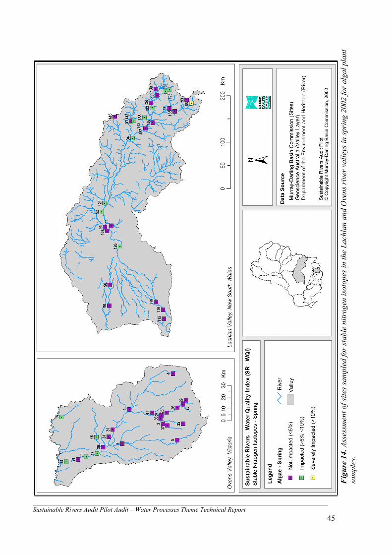
Sustainable Rivers Audit Pilot Audit – Water Processes Theme Technical Report 45
F
igur
e 14
. Ass
essm
ent o
f site
s sam
pled
for s
tabl
e ni
trog
en is
otop
es in
the
Lach
lan
and
Ove
ns ri
ver v
alle
ys in
spri
ng 2
002
for a
lgal
pla
nt
sam
ples
.

Sustainable Rivers Audit Pilot Audit – Water Processes Theme Technical Report 46
F
igur
e 15
. Ass
essm
ent o
f site
s sam
pled
for s
tabl
e ni
trog
en is
otop
es in
the
Lach
lan
and
Ove
ns ri
ver v
alle
ys in
sum
mer
200
3 fo
r alg
al p
lant
sa
mpl
es.

Sustainable Rivers Audit Pilot Audit – Water Processes Theme Technical Report
47
Quality control issues listed in Bunn and Fellows (2003) were related to the following:
• Ensuring separate collection of different types of plant material
• Correct labeling and identification of algal and vascular plants, and detailed descriptions of collected plant material
• Removal of sediment, detritus and other potential contaminants, either in the field or in the laboratory before storage.
• Only collecting submerged aquatic plants
• Adequate number of samples
In any future SRA these issues would need to be addressed by revising the sampling protocols and ensuring a sufficient level of training of field staff.
6.4.2 Assessing stable carbon isotopes against reference condition Variability in replicate samples of the same kinds of plants collected at the same sites and times is usually very low. Typically, standard errors range between 0.5 and 3.5% of the mean (Bunn and Fellows, 2003), and the data from this data set fall well within this range.
There were only a limited number of sites where both GPP data were collected and δ13C values were obtained. Therefore it was not possible to examine the relationship between both. Comparison of algae and vascular plant δ13C values was only possible for a subset of the Lachlan sites in spring and summer, and the differences were not statistically significant between both groups (Wilcoxon signed-rank test, n=11, p>0.05) (Table 14 and Table 15). In the Lachlan, δ13C values were also not significantly different between seasons for algae (mean difference = 0.9 ‰, Wilcoxon signed-rank test, n=9, p>0.05) or for vascular plants (mean difference = 0.2 ‰, Wilcoxon signed-rank test, n=11, p>0.05). In the Ovens δ13C values were significantly different between seasons for vascular plants (mean difference = 2.5 ‰, Wilcoxon signed-rank test, n=10, p>0.05). These results may be confounded by the small sample sizes and because some of the vascular plant samples were from emergent, rather than submerged plants.
6.4.3 The use of stable nitrogen isotopes as a routine indicator of river health Stable nitrogen isotopes can indicate anthropogenic impacts from surrounding land use and as such are a valuable process indicator with regard to nutrient cycling. Under natural conditions, biologically accessible nitrogen is often in short supply, limiting the production of aquatic plants and resulting in poorly buffered quantities of fixed nitrogen being available. Hence nitrogen run-off into our river systems is likely to be a contributor to phytoplankton blooms in the water column, in particular of species that are not able to fix nitrogen from the atmosphere. The dynamics of this are complex and depend on variables such as flow regime, light availability, turbidity, macrophyte and filamentous algal nitrogen uptake and ‘seeding’ blue green algal populations present in the water column. Ford (2003) concludes that δ15N is not a direct indicator of river health but useful in detecting large scale anthropogenic inputs and perturbance from its natural state. He concludes that despite its inability to differentiate between nitrogen input resulting from agricultural land use and inputs of human waste it may be important to establish a baseline of δ15N values to monitor foreshadowed changes in agriculture leading to a higher use of synthetic nitrogen fertilizers. However, establishing a δ15N baseline with regard to impacts from surrounding land use would involve a research component that is outside the scope of the Sustainable Rivers Audit. Bunn and Fellows (2003) also recommend using this indicator, and suggest the collection of primary consumers (grazers) in addition to filamentous algal material and the integration of the information over a larger time scale.

Sustainable Rivers Audit Pilot Audit – Water Processes Theme Technical Report
48
The Pilot study has highlighted that despite some strong evidence of correlations between land use and nitrogen isotope signatures, the use of stable isotope ratios as an indicator is not ready for routine incorporation into a monitoring program. Further method development should elucidate:
• A tighter definition of the relationship between land use and isotope signature by accounting for non-explained variability, investigating spatial and temporal scales at which the correlation operates (land area to sampling point, time scales over which the relationship operates for producers and primary consumers)
• A more refined classification of reference condition and departure
• Implications of the indicator on in-stream river health, in particular a better understanding of the N cycle and its implications for ecosystem processes
Isotope ratios can be collected at relatively low cost, compared to other water quality and water processes indicators. Method development requirements for indicators are in itself no impediment for adopting an indicator for the SRA, but for this indicator the method development is partly dependent on the additional collection of data for other water processes indicators and on the availability of data on catchment land use in the appropriate format. Interpretation of the indicator appears to be complex and not entirely relevant to in-stream river health per se, so its inclusion would be dependent on the adoption of other indicators for the water processes theme.
6.4.4 The use of stable carbon isotopes as a routine indicator of river health Defining reference condition for this indicator is biome specific and in order to understand the complex pathways of the isotope ratios, substantial research would be required. Ford (2003) suggests that δ13C values are potentially influenced by extraneous factors that cannot reliably be used in the assessment of river health. Bunn and Fellows (2003) conclude that although there is a relatively strong relationship between algal δ13C and benthic GPP at a regional scale the indicator is not a robust surrogate for measuring GPP, but could be used at the extreme ends of the range to check GPP measurements. Collecting information on δ13C values would appear to be useful for further research projects, and since analysis of samples for δ13C values can be done at virtually no extra cost it could be included with the former. However, apart from checking GPP measurements at the extreme end its usefulness as an indicator is not clear at this stage and further research is needed in this regard. Inclusion of stable isotopes (C and N) would be made dependent on the adoption of other indicators for the water processes theme.
6.5 Power analysis Bunn and Fellows (2003) recommend the collection of only algal plant material (to avoid collection of emergent vascular plants not suitable for analysis) and where possible primary consumers (grazers) of these plants. For this reason, the power analysis was only conducted on the results for algae and not for vascular plants. The mean and standard deviation of the values for N stable isotopes were used, since this is the indicator recommended to be adopted and further developed. While values for C isotope ratios may be used to check data on GPP, the aim to establish confidence levels for this indicator would not be pursued unless it would be decided to further develop it in order to gauge relative contributions to river flows from groundwater influx. For the Lachlan, to detect a level of change of 0.1 with confidence α = 0.05 and power = 0.8, 17 samples were required, and for the Ovens 27. Therefore, it is anticipated that if samples could be collected at each macroinvertebrate sampling site, sufficient samples would be available to detect a 0.1 level change at the valley level.

Sustainable Rivers Audit Pilot Audit – Water Processes Theme Technical Report
49
7 Water quality spot measurements
7.1 Methods
7.1.1 Site selection and layout Sites were selected and sampled according to the protocol (see APPENDIX 3) and involved a limited number of ‘best available’ sites and a larger number of assessment sites. Criteria for best available sites are listed in APPENDIX 4; site selection of assessment sites was undertaken maximising parity with fish sampling sites since there are no specific criteria related to water quality sampling other than accessibility. Figure 16 shows the location of water quality sampling sites for the Pilot project (see Figure 2 for delineation of VPZ’s in the Basin). The list of sites and their location is presented in APPENDIX 4. These sites are a subset of fish and/or macroinvertebrate sampling sites. The number of sites required for the SRA depends on the:
• spatial reporting scale of the assessment
• variability of the indicator
• initial condition score of the indicator
• aggregation and reporting statistics used
• desired level of change to be detected
• desired confidence in detecting that change. It was decided to use the macroinvertebrate and fish sites to undertake sampling for spot measurement indicators in order to minimise costs associated with the sampling. The number of sites would adequately cover the Framework report recommendation for proposed number of sites for sampling for water quality, where 9 sites were suggested per VPZ (3 best available and 6 assessment sites).
7.1.2 Assessment sites The number of assessment sites for the Pilot Audit has been chosen with various considerations across the themes. One of the objectives of the Pilot is to provide data to determine the appropriate ‘effect size’ and hence sample size for the full SRA. Power analyses have informed the decision of the number of sites, particularly for the fish and macroinvertebrate themes, but practical issues (time and costs) also needed to be considered. Another important issue is parity in site locations across themes. A desire to collect the most informative set of data has led to the decision to have as much site overlap as possible between themes – at least for the Pilot Audit. The hydrology, physical habitat and water quality themes are also intended to assist with the interpretation of the biotic indicators, so in general it will be useful to have this information at as many sites as possible where macroinvertebrates or fish are sampled.
Taking these issues into consideration, sampling for physico-chemical spot measurements were done at macroinvertebrate and fish sampling sites, but other sites were included as well, resulting in 166 sites across the four Pilot valleys (Condamine 38, Lachlan 43, Ovens 43 and Lower Murray 42). Fish and macroinvertebrate sites were assessed using the criteria for ‘best available’ for water quality spot measurements and the specifications listed in the sampling protocols (APPENDIX 3)
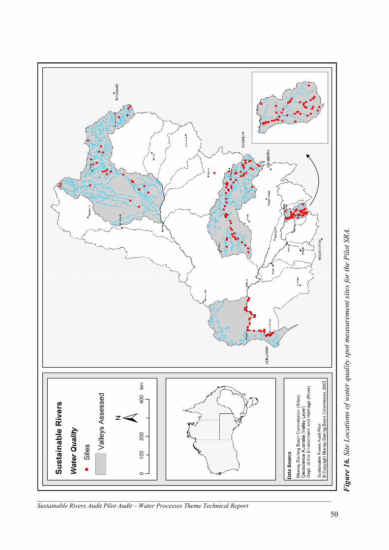
Sustainable Rivers Audit Pilot Audit – Water Processes Theme Technical Report 50
F
igur
e 16
. Site
Loc
atio
ns o
f wat
er q
ualit
y sp
ot m
easu
rem
ent s
ites f
or th
e Pi
lot S
RA.

Sustainable Rivers Audit Pilot Audit – Water Processes Theme Technical Report
51
7.1.3 Best available sites The construction of reference condition by an expert group used information from any of the following sources to determine the range of expected natural conditions for each VPZ:
• Data from best available sites
• Historical data/observations
• Data from sites other than specially selected best available sites
• Conceptual or numerical modelling
• Literature and expert knowledge. Reference condition was ‘constructed’ to overcome the problem of there not being sites which can be accepted as being in natural condition (this is especially true in lowland areas). For the water processes theme, it was expected that the majority of the construction of reference would be based on expert knowledge and existing data, with only a few ‘best available’ sites being sampled. Only in the Lachlan and the Condamine valleys a number of best available sites were identified. Best available sites were selected by identifying potential good quality sites (using existing datasets or local knowledge) and then ranking these potential sites using the matrix in Table 16. This was done by multiplying the influence weighting by the disturbance rating. The lowest scoring sites are used as ‘best available’ sites; a total of 33 (16.5% of all water quality sites across the four valleys) were selected in the Lachlan (17) and Condamine (16). Note that the disturbance and influence categories in this table are the same used to evaluate the best available fish sites and only the weightings have been changed.
7.1.4 Sampling frequency, season and condition at sites As sampling was undertaken in ‘stable’ conditions it occurred during base-flow rather than flood-flow. Sample protocols were followed for dealing with dry sites (see APPENDIX 3) and samples were collected during winter 2002 (limited sites), spring 2002 and summer 2003.
7.1.5 Data formatting Any data point that was listed as below detectable limit was set to 0.0005 -half the below detectable limit. Where there was more than one replicate the average was calculated for each variable for each site. For the Pilot study, all incomplete data sets are included in the analyses.
7.2 Results and discussion The results of nine indicators (temperature, conductivity, pH, dissolved oxygen (percent saturation), turbidity, total phosphorus, total nitrogen, NOx and pelagic chlorophyll-a) have been presented for best available sites and for assessment sites. The data have been graphed as median, with 20th and 80th percentiles for each of the VPZ’s, and reference condition values have been indicated on the graphs.
7.2.1 Best available sites Best available sites were only available in the Condamine and Lachlan VPZ’s; no data could be presented on the other two Pilot valleys. Within the Condamine and Lachlan the data are compared with the reference values determined by the reference reconstruction group; it would be expected that most data would fall within the reference boundaries as determined under section 4.3.

Sustainable Rivers Audit Pilot Audit – Water Processes Theme Technical Report
52
Table 16. Rating system for assessing human disturbance at potential reference/best available water process sites
Disturbance High influence = 3 Medium influence = 2
Low influence = 1
[Manufacturing] Industry includes factories, mining, power plants Weighting = 3
Industrial areas adjacent to the site or close upstream (< about 20km); industrial discharges enter the stream
Substantial industrial areas in the catchment but not close to the site
No industrial areas in catchment (small catchments) or industrial areas remote from the site and a minuscule proportion of catchment area (large catchments)
Urbanization Weighting = 3
Site lies within or close downstream of high-density urban area; urban drainage or sewage discharge enters the stream
Substantial urban areas in the catchment but not close to the site; or low-density urban areas only near the site, without direct drainage or discharge
No urban areas in catchment (small catchments) or urban areas remote from the site and a minuscule proportion of catchment area (large catchments)
Irrigated Cropping Weighting = 3
Large irrigated cropping areas (e.g. horticulture, cotton, rice farms) adjacent to the site or close upstream; tailwater drainage enters the stream
Substantial cropping areas in the catchment but not close to the site
No cropping in catchment (small catchments) or cropping remote from the site and a minuscule proportion of catchment area (large catchments)
Dryland cropping / riparian Weighting = 1
Large dryland cropping areas (e.g. wheat, oilseeds farms) adjacent to the site or close upstream;
Substantial dryland cropping areas in the catchment but not close to the site
No dryland cropping in catchment (small catchments) or cropping remote from the site and a minuscule proportion of catchment area (large catchments
Grazing / riparian Weighting = 2
Riparian zone intensively grazed; faeces, pug-marks, eroded access tracks, or chewing down of vegetation conspicuously present
Riparian zone ungrazed or lightly grazed, but substantial riparian grazing near site, close upstream or through much of catchment
No grazing in catchment (small catchments) or grazing areas remote from the site and a small proportion of catchment area (large catchments)
Recreation Weighting = 0
Clear evidence of recreational use, e.g. people present, trampling, litter, fishing lines
No clear evidence of recreation but accessibility suggests some use is likely
Site unlikely to be accessed for recreation
Water extraction Weighting = 2
Large irrigation districts upstream of the site; total flow volume greatly reduced
Only localised irrigation upstream of the site; total flow volume not greatly reduced but substantial portion of low flow may be extracted
Little or no extractive use upstream of the site
Flow regulation Weighting = 2
Seasonal or diel pattern of flows greatly altered by upstream storage and release patterns
Upstream impoundment alters diel or seasonal flow pattern, but unregulated tributary flows result in substantial normalization
No significant upstream impoundment
Hypolimnetic release Weighting = 3
Bottom-release dam <150km upstream; summer temperatures substantially below natural; winter temperatures may be elevated
Bottom-release dam upstream but >150km distant from site; seasonal temperature regime only moderately altered
No significant upstream impoundment or upstream impoundment with effective multi-level offtake
Artificial barriers Weighting = 1
High barriers <150km downstream of the site, likely to be severely constraining fish migration
Barriers are likely to be affecting migration to/from the site but they are low or distant from the site
Any barriers are upstream and remote from the site.
Alien fish Weighting = 1
Alien fish dominate the site in terms of either numbers or biomass
Alien fish present but do not dominate
No alien fish at the site
Alien plants Weighting = 0
Riparian zone has lost most or all of original tree and shrub cover; riparian and aquatic vegetation dominated by alien species
Riparian zone retains native trees and shrubs but substantial alien vegetation present. Aquatic plants predominantly native
Riparian and aquatic vegetation not cleared. Little or no alien plant invasion
Geomorphic change Weighting = 1
Poor geomorphic condition (River Styles™ or similar method)
Moderate geomorphic condition (River Styles™ or similar method)
Good geomorphic condition (River Styles™ or similar method)
7.2.1.1 Temperature Best available sites appear to reveal temperatures on the higher end of the reference boundaries (Figure 17). It is possible that this is a result of measurements made under extreme draught conditions. It should be noted that reference boundaries have been set very wide (band between 10-15 degrees difference) which makes their use as reference questionable. The approach of determining reference on a VPZ scale is unlikely to be valid for this reason, and reference

Sustainable Rivers Audit Pilot Audit – Water Processes Theme Technical Report
53
condition may need to be determined at the site level scale, taking into account time of day and season. This is usually done by setting limits on ∆T and using an unimpacted site as reference. This would change the VPZ assessment to a percentage site compliance approach which requires a much larger number of sites to obtain a representative assessment at the VPZ scale. The use of reference condition to assess potential thermal pollution would probably also require consideration of additional data on ambient air temperature. This is more likely a localised problem that needs to be monitored by investigative monitoring where sites are selected according to monitor upstream and downstream of well known impacts, rather than the random site selection used for the SRA. Assessing the overall condition at the VPZ level in terms of departure from reference for temperature would require further method development to define:
• greater precision in defining reference, accounting for seasonal differences
• the spatial and temporal scale of a measurement representative
• aggregation of measured results
0
5
10
15
20
25
30
Condaminedeposition
Condaminetransport
Condaminesource
Lachlandeposition
Lachlansource
Tem
pera
ture
(Deg
ree
Cel
cius
)
medianLow refHigh ref
Figure 17. Temperature results from Pilot data for best available sites (median and 20th and 80th percentiles, denoted by whiskers), with low and high reference values.
7.2.1.2 Conductivity The Condamine transport VPZ has reference values that are set very high, and the data from best available appear to lie in a much narrower band at much lower values (Figure 18). The opposite is the case for the Condamine source VPZ. Geographically, the two VPZ have little in common and different reference conditions are not surprising, but given the wide reference band for Condamine transport it is unusual to find best available sites having much lower conductivity values. The reference conditions for Condamine transport zone were based on percentiles calculated by the Department of Natural Resource Management for that particular area (Figure 6), using 283 sites (Heather Hunter, pers. com., 2003). The Lachlan appears to have high variability at best available sites, which is reflected in the reference upper and lower limits, despite the observed values exceeding the upper boundaries.
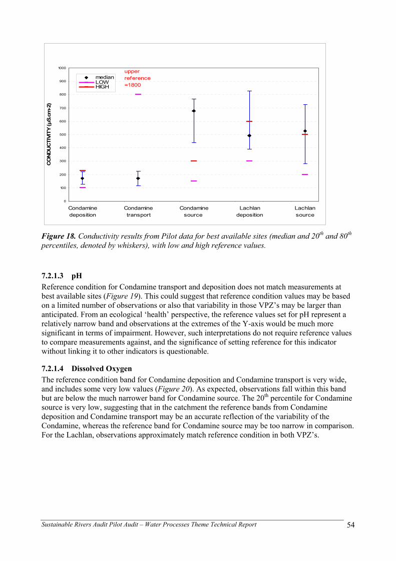
Sustainable Rivers Audit Pilot Audit – Water Processes Theme Technical Report
54
0
100
200
300
400
500
600
700
800
900
1000
Condaminedeposition
Condaminetransport
Condaminesource
Lachlandeposition
Lachlansource
CO
ND
UC
TIVI
TY (µ
S.cm
-2)
medianLOWHIGH
upper reference =1800
Figure 18. Conductivity results from Pilot data for best available sites (median and 20th and 80th percentiles, denoted by whiskers), with low and high reference values.
7.2.1.3 pH Reference condition for Condamine transport and deposition does not match measurements at best available sites (Figure 19). This could suggest that reference condition values may be based on a limited number of observations or also that variability in those VPZ’s may be larger than anticipated. From an ecological ‘health’ perspective, the reference values set for pH represent a relatively narrow band and observations at the extremes of the Y-axis would be much more significant in terms of impairment. However, such interpretations do not require reference values to compare measurements against, and the significance of setting reference for this indicator without linking it to other indicators is questionable.
7.2.1.4 Dissolved Oxygen The reference condition band for Condamine deposition and Condamine transport is very wide, and includes some very low values (Figure 20). As expected, observations fall within this band but are below the much narrower band for Condamine source. The 20th percentile for Condamine source is very low, suggesting that in the catchment the reference bands from Condamine deposition and Condamine transport may be an accurate reflection of the variability of the Condamine, whereas the reference band for Condamine source may be too narrow in comparison. For the Lachlan, observations approximately match reference condition in both VPZ’s.

Sustainable Rivers Audit Pilot Audit – Water Processes Theme Technical Report
55
5
6
7
8
9
10
Condaminedeposition
Condaminetransport
Condaminesource
Lachlandeposition
Lachlansource
pH
medianLOWHIGH
Figure 19. pH results from Pilot data for best available sites (median and 20th and 80th percentiles, denoted by whiskers), with low and high reference values.
0
10
20
30
40
50
60
70
80
90
100
110
120
130
140
Condaminedeposition
Condaminetransport
Condaminesource
Lachlandeposition
Lachlansource
DO
(%sa
t)
medianLOWHIGH
Figure 20. Dissolved Oxygen (% saturation) results from Pilot data for best available sites (median and 20th and 80th percentiles, denoted by whiskers), with low and high reference values.

Sustainable Rivers Audit Pilot Audit – Water Processes Theme Technical Report
56
7.2.1.5 Turbidity Turbidity values had to be represented on a logarithmic scale, due to the enormous differences between VPZ’s (Figure 21). In particular, Condamine transport and Condamine deposition have very high turbidity values, even during baseline flow. Although reference conditions were determined to reflect this, the observations for best available sites are still higher than reference. The wide range of reference may be a case for attempting to narrow down reference according to season or smaller reach scales to increase precision of a potential assessment. For the Lachlan the upper limits of reference reflects measurements at best available sites, whereas at the lower end best available sites appear to indicate lower turbidities than what was determined for reference sites. However, turbidity values of < 10 NTU are so low that the lower reference bounds are becoming insignificant.
1
10
100
1000
Condaminedeposition
Condaminetransport
Condaminesource
Lachlandeposition
Lachlansource
TURBID
ITY
(NTU
medianLOWHIGH
Figure 21. Turbidity results from Pilot data for best available sites (median and 20th and 80th percentiles, denoted by whiskers), with low and high reference values. Y-axis is on a logarithmic scale.
7.2.1.6 Total Phosphorus Total phosphorus values and reference boundaries are high in the Condamine compared to the Lachlan (Figure 22). This would reflect the high turbidities associated with variable flow events. In the Condamine source, the observed values are well above the reference for that VPZ, whereas for most other VPZ’s the values at best available sites approximately reflect the reference condition boundaries.
7.2.1.7 Total Nitrogen The upper limit on the reference condition of Condamine transport (Ur = 7.3) appears to be too high to be a realistic reference boundary, compare to all other values for nutrients (Figure 23). If this is based on 80th percentiles from Condamine datasets, it would imply that the limited observations at best available sites are at the lower end of the scale. The reference bands for Condamine source and Condamine deposition are still very wide but this is consistent with reference values for other indicators in those VPZ’s. The reference values for the Lachlan are lower and narrower bands, but the values for best available sites exceed the upper reference boundaries.
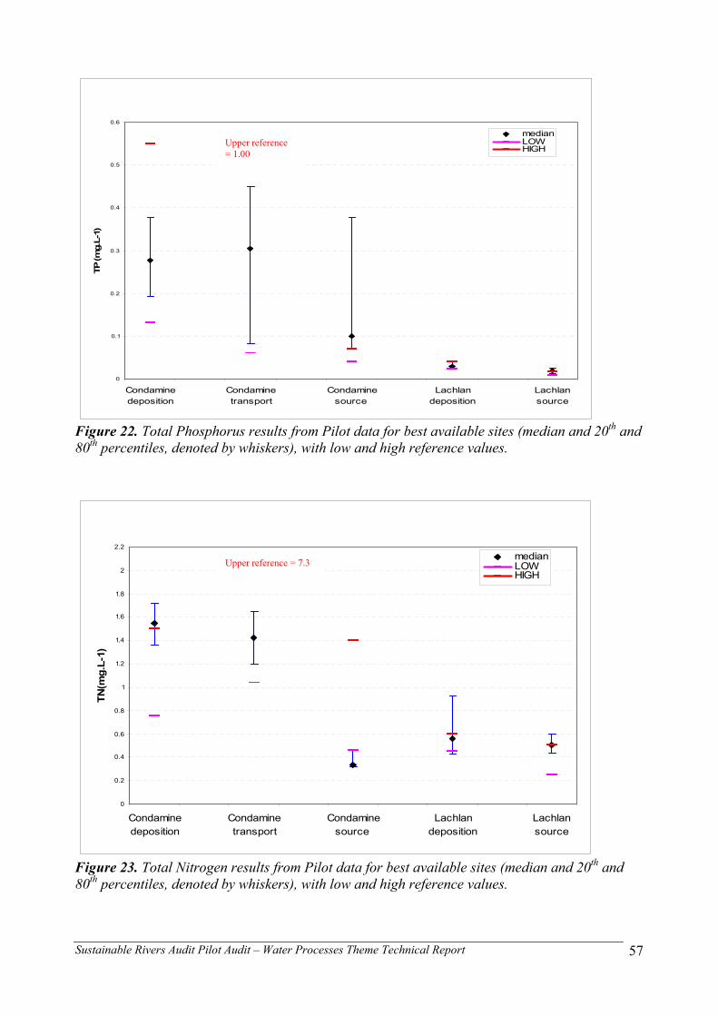
Sustainable Rivers Audit Pilot Audit – Water Processes Theme Technical Report
57
0
0.1
0.2
0.3
0.4
0.5
0.6
Condaminedeposition
Condaminetransport
Condaminesource
Lachlandeposition
Lachlansource
TP (m
g.L-
1)
medianLOWHIGH
Figure 22. Total Phosphorus results from Pilot data for best available sites (median and 20th and 80th percentiles, denoted by whiskers), with low and high reference values.
0
0.2
0.4
0.6
0.8
1
1.2
1.4
1.6
1.8
2
2.2
Condaminedeposition
Condaminetransport
Condaminesource
Lachlandeposition
Lachlansource
TN(m
g.L-
1)
medianLOWHIGH
Figure 23. Total Nitrogen results from Pilot data for best available sites (median and 20th and 80th percentiles, denoted by whiskers), with low and high reference values.
Upper reference = 1.00
Upper reference = 7.3

Sustainable Rivers Audit Pilot Audit – Water Processes Theme Technical Report
58
7.2.1.8 NOx Extreme variability characterises NOx levels in the Condamine, contributing to the variability of TN (Figure 24). Reference condition appears set at levels reflecting best available sites, despite the low values found in Condamine source. In the Lachlan values are much lower and reference condition has been defined accordingly.
0
0.05
0.1
0.15
0.2
0.25
0.3
0.35
0.4
Condaminedeposition
Condaminetransport
Condaminesource
Lachlandeposition
Lachlansource
Nox
N (m
g.L-
1)
medianLOWHIGH
Figure 24. NOx results from Pilot data for best available sites (median and 20th and 80th percentiles, denoted by whiskers), with low and high reference values.
7.2.1.9 Chlorophyll-a Chlorophyll-a reference values in Condamine deposition and Condamine transport would suggest that under natural conditions, levels are sufficiently low to impede major algal blooms, given the high turbidity levels which would limit light availability (Figure 25). The results from best available sites suggest otherwise and this may indicate that best available does not reflect natural very well. In the Lachlan, values for best available sites are below the lower boundary of reference condition suggesting that conditions for phytoplankton growth are not favourable. It could be argued that lower boundaries for this indicator should be zero instead of the 20th percentile, as natural variability in the valley zones would suggest there are instances where zero values are possible.

Sustainable Rivers Audit Pilot Audit – Water Processes Theme Technical Report
59
0
5
10
15
20
25
30
35
40
45
50
Condaminedeposition
Condaminetransport
Condaminesource
Lachlandeposition
Lachlansource
CH
LOR
OPH
YLL-
a (u
g.L-
1)
medianLOWHIGH
Figure 25. Chlorophyll-a results from Pilot data for best available sites (median and 20th and 80th percentiles, denoted by whiskers), with low and high reference values.
7.2.2 Assessment sites All four Pilot valleys were assessed in the same seasons as for best available sites (Spring 2002 and Summer 2003), but the latter were only available for the Lachlan and the Condamine. Table 4 presents the number of sites sampled in each VPZ for water quality spot measurements.
7.2.2.1 Temperature Except for Ovens source, temperature ranges for reference condition are very wide for all VPZ’s (Figure 26). This would have the effect of most observations being near natural, and will not provide for a very sensitive analysis of condition. Compared to best available sites, very little differences can be detected in observed values. All readings are at the higher scale of the reference condition, which may be explained by the fact that sampling took place during an extreme draught. As discussed under 7.2.1.1, using ∆T at the site may be a better way of refining reference condition, provided that the site information can be integrated to the VPZ scale other than using the percent compliance approach (which would require too numerous sites to be practicably feasible and cost effective).
7.2.2.2 Conductivity Conductivity ranges are large except for Ovens deposition and Ovens source (Figure 27). There is a substantial difference in observed values between assessment sites and best available for Condamine deposition, Condamine source and Lachlan source, where values for assessment sites are much higher. It is noteworthy that the reference values for Condamine transport are set much higher than the recorded values for both best available and assessment sites, whereas in the Condamine source the opposite is the case. Values for Lachlan deposition are similar between best available and assessment sites, both exceeding the upper boundary of the reference value. A possible explanation for these high values may be that during extreme draught, groundwater intrusions are responsible for the higher conductivity (salinity) levels. Note that the scale for this graph was set at identical range than for best available sites, resulting in values for Condamine deposition, Condamine transport and Condamine source being off the scale.
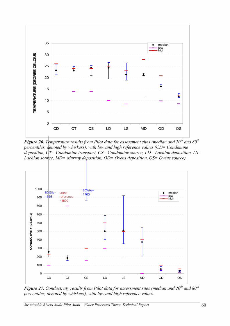
Sustainable Rivers Audit Pilot Audit – Water Processes Theme Technical Report
60
0
5
10
15
20
25
30
35
CD CT CS LD LS MD OD OS
TEM
PERA
TUR
E (D
EGR
EE C
ELC
IUS
medianlowhigh
Figure 26. Temperature results from Pilot data for assessment sites (median and 20th and 80th percentiles, denoted by whiskers), with low and high reference values (CD= Condamine deposition, CT= Condamine transport, CS= Condamine source, LD= Lachlan deposition, LS= Lachlan source, MD= Murray deposition, OD= Ovens deposition, OS= Ovens source).
0
100
200
300
400
500
600
700
800
900
1000
CD CT CS LD LS MD OD OS
CO
ND
UC
TIVI
TY (µ
S.cm
-2)
medianlowhigh
80%ile=1625
80%ile=1703upper
reference =1800
Figure 27. Conductivity results from Pilot data for assessment sites (median and 20th and 80th percentiles, denoted by whiskers), with low and high reference values.

Sustainable Rivers Audit Pilot Audit – Water Processes Theme Technical Report
61
7.2.2.3 pH The pH values in Condamine deposition are exceeding the reference boundaries at both ends, and indicate that there is a large variability in pH for this VPZ (Figure 28). Except for Condamine transport and Ovens source, other values for assessment sites all lie within the reference boundaries. Condamine transport values are below reference, as for best available sites, whereas Ovens transport values are exceeding the upper limit but are in a similar range to values observed for Ovens deposition.
5
6
7
8
9
10
CD CT CS LD LS MD OD OS
pH
medianlowhigh
Figure 28. pH results from Pilot data for assessment sites (median and 20th and 80th percentiles, denoted by whiskers), with low and high reference values.
7.2.2.4 Dissolved Oxygen Generally observed values at assessment sites display a wider range, but are similar with regard to reference boundaries when compared with best available sites (Figure 29). One notable exception to this are the wide range of values observed for Lachlan source at assessment sites. It is difficult to compare GPP values with these DO spot measurements as it is not known if those measurements were taken on the same days. However, spot measurements for Chlorophyll-a reveal very low values (also at assessment sites, see Figure 25), suggesting that productivity in that VPZ was low at the majority of sites. This indicates a heterotrophic system with at some sites poor oxygenation.
7.2.2.5 Turbidity Trends in turbidity values for assessment sites are similar to best available, again reflecting a wide range of turbidities for the Condamine (Figure 30). In the source VPZ’s turbidities are generally lowest as would be expected.

Sustainable Rivers Audit Pilot Audit – Water Processes Theme Technical Report
62
0
10
20
30
40
50
60
70
80
90
100
110
120
130
140
CD CT CS LD LS MD OD OS
DO
(%sa
t)
medianlowhigh
Figure 29. Dissolved Oxygen (% saturation) results from Pilot data for assessment sites (median and 20th and 80th percentiles, denoted by whiskers), with low and high reference values.
1
10
100
1000
CD CT CS LD LS MD OD OS
TUR
BID
ITY
(NTU
medianlowhigh
Figure 30. Turbidity results from Pilot data for assessment sites (median and 20th and 80th percentiles, denoted by whiskers), with low and high reference values. Y-axis values are on a logarithmic scale.

Sustainable Rivers Audit Pilot Audit – Water Processes Theme Technical Report
63
7.2.2.6 Total Phosphorus Observed values for total phosphorus are generally much lower than those observed at best available sites in the Condamine (while median values are similar, the 20th and 80th percentile ranges are a lot narrower, Figure 31). Reference boundaries were selected at very high upper limits, especially for Condamine transport. The high levels of TP appear to correlate with the high turbidity levels in the Condamine transport and deposition zones. The values at assessment sites are within or just above upper reference limits, except for the Murray, where reference was exceeded. In the Lachlan, values detected at assessment sites are very similar to best available, and are approximately within defined reference.
0
0.1
0.2
0.3
0.4
0.5
0.6
CD CT CS LD LS MD OD OS
TP (m
g.L-
1)
medianlowhigh
Figure 31. Total phosphorus results from Pilot data for assessment sites (median and 20th and 80th percentiles, denoted by whiskers), with low and high reference values.
7.2.2.7 Total Nitrogen Value ranges for Condamine deposition and Lachlan source have a wider spread for assessment sites than for best available, and at Lachlan source exceed reference substantially (Figure 32). Other trends appear to be fairly similar to best available sites. Reference boundaries for Ovens and Lachlan are similar, but in the Ovens values are at the lower end of the range.
7.2.2.8 NOx In Condamine deposition, the values at assessment sites are much lower than those observed at best available sites (Figure 33). Other values appear comparable between both site categories. Ovens deposition has higher ranges than Ovens source, Lachlan deposition and Lachlan source and Murray deposition with all observed values being within the reference range. Murray deposition is the only VPZ where values exceed reference.
Upper reference = 1.00
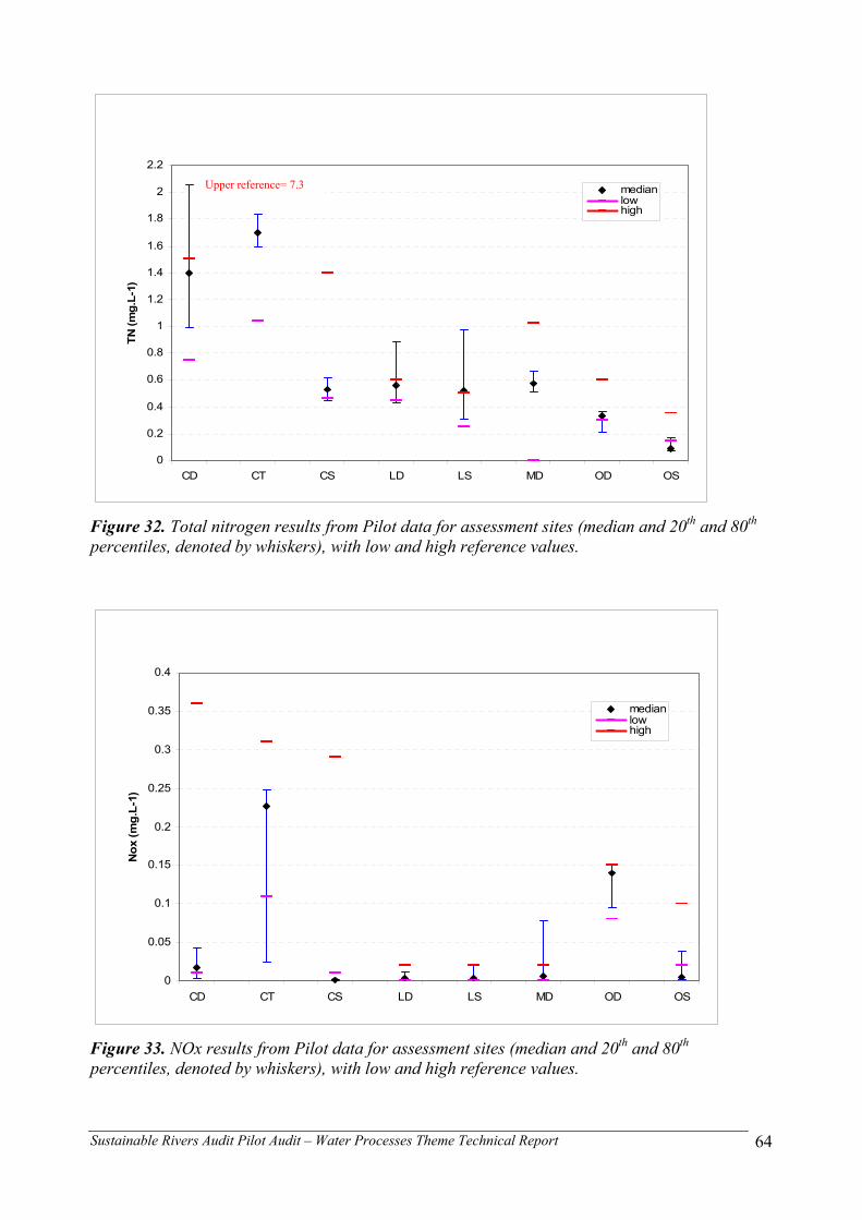
Sustainable Rivers Audit Pilot Audit – Water Processes Theme Technical Report
64
0
0.2
0.4
0.6
0.8
1
1.2
1.4
1.6
1.8
2
2.2
CD CT CS LD LS MD OD OS
TN (m
g.L-
1)
medianlowhigh
Figure 32. Total nitrogen results from Pilot data for assessment sites (median and 20th and 80th percentiles, denoted by whiskers), with low and high reference values.
0
0.05
0.1
0.15
0.2
0.25
0.3
0.35
0.4
CD CT CS LD LS MD OD OS
Nox
(mg.
L-1)
medianlowhigh
Figure 33. NOx results from Pilot data for assessment sites (median and 20th and 80th percentiles, denoted by whiskers), with low and high reference values.
Upper reference= 7.3

Sustainable Rivers Audit Pilot Audit – Water Processes Theme Technical Report
65
7.2.2.9 Chlorophyll-a In the Condamine, chlorophyll-a values exceed reference upper limits in all three VPZ’s (Figure 34). In the Condamine source and transport, values for assessment sites are higher than for best available, but for the Condamine deposition the opposite is true. In the other VPZ’s values are within or below reference (consistent with observations for best available sites), except for Murray deposition for which no data were available.
0
5
10
15
20
25
30
35
40
45
50
CD CT CS LD LS MD OD OS
CH
LOR
-a (u
g.L-
1)
medianlowhigh
no data
Figure 34. Chlorophyll-a results from Pilot data for assessment sites (median and 20th and 80th percentiles, denoted by whiskers), with low and high reference values.
As mentioned earlier, departure from reference can also be reported as percentage of sites exceeding upper or lower limits of reference. Impacts of exceeding higher limits may carry higher weight in terms of ecological importance, as would be the case for nutrients, turbidity, conductivity and chlorophyll-a. For other indicators, departure from upper or lower limit has equal implications (e.g. temperature or pH). For an overall assessment of a Sustainable River - Water Index (SR-WI), these differences would need to be combined in a rule set taking into account ecological importance of departure from reference for each of the indicators, and for the interaction amongst those. Figures 35 to 42 represent departure from reference for each of the indicators at assessment sites only as percentage of sites outside upper (red) or lower (green) limits. As can be seen from the graphs there are many parameters for which there are only very few observations (n). The results of non-compliance should therefore be interpreted with extreme caution. For example, a variable with no bar listed against it can mean 100% compliance, but can also mean no data were available for this indicator. Assessing VPZ condition based on this limited information was therefore not possible. The following section further comments on the number of required sites to detect a 10% change in percentage compliance; this number is higher

Sustainable Rivers Audit Pilot Audit – Water Processes Theme Technical Report
66
than that required when aggregating data to the VPZ level, and could therefore never achieve parity with sites sampled for other themes (fish, macroinvertebrates).
r i vpz=C-D Season=Spr i ng
cat Hi gh Low
0
10
20
30
40
50
60
70
80
90
100
measure
Turb
Temp
pH
Cond
TP
TN
DO
NOx
chlA
4
4 4 4
1
3
6
r i vpz=C-D Season=Summer
Hi gh Low
0
10
20
30
40
50
60
70
80
90
100
measure
Turb
Temp
pH
Cond
TP
TN
DO
NOx
chlA
22
4
2 2
1
2
1
5
Figure 35. Condamine deposition VPZ with percent compliance of assessment sites in Spring (left) and in Summer (right). Numbers in the bars denote number of observations (n).
r i vpz=C-S Season=Spr i ng
Hi gh Low
0
10
20
30
40
50
60
70
80
90
100
measure
Turb
Temp
pH
Cond
TP
TN
DO
NOx
chlA
1riv pz =C -S S eas on=S pr in g
Hi gh Lo w
0
102030
405060
708090
1 00
m easu re
Turb
Temp
pH
Cond
TP
TN
DO
NOx
chlA
1 11
1
r i vpz=C-S Season=Summer
Hi gh
0
10
20
30
40
50
60
70
80
90
100
measure
Turb
Temp
pH
Cond
TP
TN
DO
NOx
chlA
1
2 22
1
2 2
Figure 36. Condamine source VPZ with percent compliance of assessment sites in Spring (left) and in Summer (right). Numbers in the bars denote number of observations (n).

Sustainable Rivers Audit Pilot Audit – Water Processes Theme Technical Report
67
r i vpz=C-T Season=Spri ng
cat Hi gh Low
0
10
20
30
40
50
60
70
80
90
100
measure
Turb
Temp
pH
Cond
TP
TN
DO
NOx
chlA
2
3 3
2
1
3
r i vpz=C-T Season=Summer
cat Hi gh Low
0
10
20
30
40
50
60
70
80
90
100
measure
Turb
Temp
pH
Cond
TP
TN
DO
NOx
chlA
1
2
2
2
1
2
Figure 37. Condamine transport VPZ with percent compliance of assessment sites in Spring (left) and in Summer (right). Numbers in the bars denote number of observations (n).
r i vpz=L-D Season=Spr i ng
Hi gh Low
0
10
20
30
40
50
60
70
80
90
100
measure
Turb
Temp
pH
Cond
TP
TN
DO
NOx
chlA
11
1 2 5
11
7 9
9
16
r i vpz=L-D Season=Summer
cat Hi gh Low
0
10
20
30
40
50
60
70
80
90
100
measure
Turb
Temp
pH
Cond
TP
TN
DO
NOx
chlA
12
14
15
14
10
12
2
17
Figure 38. Lachlan deposition VPZ with percent compliance of assessment sites in Spring (left) and in Summer (right). Numbers in the bars denote number of observations (n).

Sustainable Rivers Audit Pilot Audit – Water Processes Theme Technical Report
68
r i vpz=L-D Season=Wi nt er
cat Hi gh Low
0
10
20
30
40
50
60
70
80
90
100
measure
Turb
Temp
pH
Cond
TP
TN
DO
NOx
chlA
2
1 1
2 2
r i vpz=L-S Season=Wi nt er
cat Hi gh Low
0
10
20
30
40
50
60
70
80
90
100
measure
Turb
Temp
pH
Cond
TP
TN
DO
NOx
chlA
11
2
1 1 1
Figure 39. Lachlan deposition VPZ with percent compliance of assessment sites in Winter (left) and Lachlan source VPZ with percent compliance of sites in Winter (right). Numbers in the bars denote number of observations (n).
r i vpz=L-S Season=Spr i ng
cat Hi gh Low
0
10
20
30
40
50
60
70
80
90
100
measure
Turb
Temp
pH
Cond
TP
TN
DO
NOx
chlA
6
2 3
4
4 4
4
6
r i vpz=L-S Season=Summer
Hi gh Low
0
10
20
30
40
50
60
70
80
90
100
measure
Turb
Temp
pH
Cond
TP
TN
DO
NOx
chlA
3
5
3
6 7
6 7
1
8
Figure 40. Lachlan source VPZ with percent compliance of assessment sites in Spring (left) and in Summer (right). Numbers in the bars denote number of observations (n).
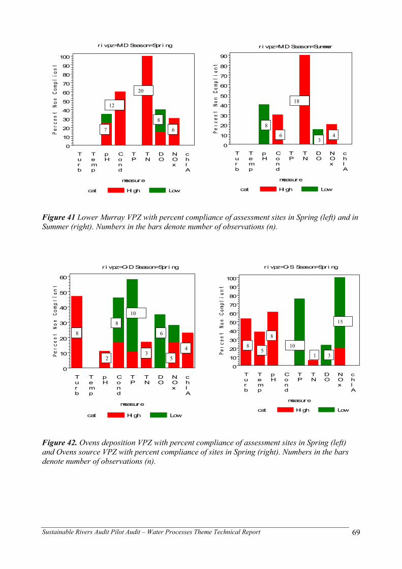
Sustainable Rivers Audit Pilot Audit – Water Processes Theme Technical Report
69
r i vpz=M-D Season=Spr i ng
cat Hi gh Low
0
10
20
30
40
50
60
70
80
90
100
measure
Turb
Temp
pH
Cond
TP
TN
DO
NOx
chlA
7
12
20
8
6
r i vpz=M-D Season=Summer
cat Hi gh Low
0
10
20
30
40
50
60
70
80
90
measure
Turb
Temp
pH
Cond
TP
TN
DO
NOx
chlA
8
6
18
3 4
Figure 41 Lower Murray VPZ with percent compliance of assessment sites in Spring (left) and in Summer (right). Numbers in the bars denote number of observations (n).
r i vpz=O-D Season=Spri ng
cat Hi gh Low
0
10
20
30
40
50
60
measure
Turb
Temp
pH
Cond
TP
TN
DO
NOx
chlA
8
2
8
10
3
6
5
4
r i vpz=O-S Season=Spr i ng
cat Hi gh Low
0
10
20
30
40
50
60
70
80
90
100
measure
Turb
Temp
pH
Cond
TP
TN
DO
NOx
chlA
85
8
10
1 3
15
Figure 42. Ovens deposition VPZ with percent compliance of assessment sites in Spring (left) and Ovens source VPZ with percent compliance of sites in Spring (right). Numbers in the bars denote number of observations (n).

Sustainable Rivers Audit Pilot Audit – Water Processes Theme Technical Report
70
7.3 Power analysis The results from the Pilot study suggest that there is a broad overlap between upland and lowland areas, and for some valleys and indicators the differences between VPZ’s are not very pronounced. Variability between valleys is often greater than between upland and lowland zones of the same valley. However, other more extensive datasets, historical knowledge and expert knowledge suggest that upland and lowland stratification is justified and reference condition will need to be defined for each of the VPZ’s. The preliminary approach to a power analysis was taking the upland and lowland stratification into account. Two measures of distance from reference were calculated:
- the average value of the 9 measures (Turbidity, Temperature, pH, Conductivity, TN, TP, DO, NOX, Chlorophyll-a, see Expert rules)
average raw distance reference = mean of (measure1 - measure9)
- the Euclidean distance of the site from a site having all 1’s (reference score)
n distance reference = n of (measure1 - measure 9);
average
Euclidean distance reference = reference distancen
9) measure distance - measure1 (distance∑
Naturally the two measures are related (Figure 43). However Euclidean distance doesn’t have as great a range as raw distance, and Spring appears to have a wider range than Summer for both assessment and best available sites. The correlation between the 9 indicators for best available and assessment sites show only weak relationships (Table 17). This suggests that indicators are fairly independent from each other and redundancy is non-existent. Hence a power analysis undertaken for the average value will not reflect confidence levels for each of the indicators separately, and further analysis is required to detect a change in the mean value for each of the indicators. Using the results in Table 17 a power analyses was initially done on the average distance (raw and Euclidean) from reference within each VPZ and within each season, but only using data from assessment sites (Figure 44). Since Euclidean distance is dependent on the way reference condition is determined, it is more conservative to base required number of sites on raw distance, despite its wider spread. The analysis was also undertaken on the values for each of the indicators separately. The graphs for each of the indicators and seasons are presented in Appendix 6. The number of sites required to detect a 10%, 20%, 30% or 40% change with α = 0.05 and β = 0.2 are given in the summary table below (Table 18). Although it could be argued that when more data are progressively being collected fewer sites are required, the design of a sampling program will always need to start out by estimates derived from limited trials so that an estimate can be made of the confidence of the initial results. The recommendations for any future SRA sampling program would emphasise the collection of samples at frequencies sufficient to pick up trends. In order to limit the number of required field

Sustainable Rivers Audit Pilot Audit – Water Processes Theme Technical Report
71
00.10.20.30.40.50.60.70.80.9
1
0 0.1 0.2 0.3 0.4 0.5 0.6 0.7 0.8 0.9 1
Average Raw Distance
Ave
rage
Euc
lidea
n D
ista
nce
Figure 43. Relationship between two measures of distance from natural for water quality measures. Hollow symbols = assessment sites, solid symbols = best available sites, circles are Spring, triangles are Summer.
Table 17. Spearman rank correlations between the 9 indicators in best available and assessment sites (n=185). Values given in bold are significant at α = 0.05 level.
Temp pH Cond TN TP DO(%sat) NOx Chl-a Turb 0.17 0.01 0.06 0.19 -0.12 0.23 0.15 0.34 Temp 0.06 0.14 0.16 -0.14 0.16 -0.06 0.25
pH 0.22 -0.05 -0.03 -0.11 0.19 0.01 Cond 0.10 0.23 0.23 0.15 0.21 TN -0.09 0.20 0.08 -0.10 TP 0.13 -0.08 0.30
DO(%sat) 0.06 0.20 NOx -0.06

Sustainable Rivers Audit Pilot Audit – Water Processes Theme Technical Report
72
Season=Spring
rivpz C-D L-D L-S M-D O-D O-S
1
10
100
diff1
0.10 0.15 0.20 0.25 0.30 0.35 0.40
Figure 44. Power analysis WP indicators average raw distance test sites only for detection of change at 0.1, 0.2, 0.3 and 0.4 levels. A minimum of 5 samples was used, VPZ with less samples were not included. Coloured lines denote different VPZ’s. Y-axis sample size is on a logarithmic scale.
Table 18. Summary table for number of sites required to detect a level of change of 0.1, 0.2, 0.3 at the VPZ level, based on VPZ with highest number of sites required, for both spring and summer.
sprin
g
av ra
w
av e
ucl
turb
idity
Tem
p
pH
Con
d
TN
TP
DO
NO
X
Chl
-a
0.1 40 20 1100 25 12 1100 500 1100 180 4000 1000 0.2 12 7 500 9 5 300 150 300 50 900 300 0.3 8 5 200 5 150 60 180 20 400 100 0.4 5 130 80 35 80 16 250 70
sum
mer
av ra
w
av e
ucl
turb
idity
Tem
p
pH
Con
d
TN
TP
DO
NO
X
Chl
-a
0.1 30 12 350 20 5 200 200 270 80 2200 500 0.2 10 5 80 8 60 60 70 20 600 110 0.3 7 40 5 30 30 30 10 250 60 0.4 5 30 20 20 20 8 170 35
visits, it is proposed to restrict sampling to a critical season where base-flow conditions exist, i.e. summer (i.e. four to six months/year) and sample for six times during this period. Using Table 18, it was suggested to sample at 35 sites per valley, to follow the recommendations for the macroinvertebrate theme, and report confidence at the valley scale instead of at the VPZ scale. Extrapolating the results of the power analysis to the valley scale level would give a confidence level of detecting a change of 10% on average. This detection level was decided arbitrarily and is consistent with the levels determined for the other SRA themes. It is a rather small change given the huge variability of some of the indicators, but since this is based on the average of all nine

Sustainable Rivers Audit Pilot Audit – Water Processes Theme Technical Report
73
indicators we feel that this is justified, as for some indicators the level at which change that can be detected is much larger. Subsequent site visits would of course increase the confidence rapidly, but it would take 2 years sampling in summer to detect a trend for indicators such as conductivity, turbidity and TP at the 20% level. A 6 year reporting cycle would therefore account for greater variabilities in the Basin and still provide adequate trend detection at the valley level. By way of comparison, the Framework report recommended 18 sites to be sampled per River Valley to detect a difference of 0.2 with a power of 0.8 and significance level of 0.1, sampled 6 times per annum. For trend detection it is proposed to carry out a power analysis after a first 6 year cycle of collecting data. In a trend analysis of the first five years of data (Robinson et al., 1994), which used a non-parametric statistical test for trend, changes smaller than 20% per annum were detectable for all indicators using monthly data. A power analysis for compliance monitoring (percentage of assessed sites per VPZ complying) was also completed using the average means and standard deviations from all 9 indicators. The results would indicate that in some cases over 200 sites would be required to detect a change of 10% (Table 19) This number is seen as exceeding the limits imposed by cost and logistics of the program. It is clear that this approach would require substantially larger numbers of sites while only still providing confidence in change for the average of all indicators, with little confidence in a change for each of the indicators separately. The information is not a very accurate measure of departure from reference, because sites may vary between VPZ’s and the percentage departure is directly depending on total number of sites monitored. Because of the large number of sites required, this approach is not recommended.
Table 19. VPZ and number of sites required for a compliance type monitoring approach, to detect change at a level of 0.1 with α = 0.05 and β = 0.2
VPZ # of sites Condamine Deposition 83 Condamine Source 58 Condamine Transport 98 Lachlan Deposition 33 Lachlan Source 47 Murray 25 Ovens Deposition 225 Ovens Source -
Sustainable Rivers Audit Pilot Audit – Water Processes Theme Technical Report
74
8 Assessing all indicators against suitability criteria The Pilot used the best collective expert scientific knowledge to select the water processes indicators to trial in the Pilot. Recommendations as to which indicators should form part of the ongoing Audit were made by considering the results from the Pilot Audit and conceptually assessing the indicators against a set of criteria derived from the US EPA’s Environmental Monitoring and Assessment (EMAP) program. The EMAP criteria have been adapted for the SRA and are used to consider the conc90ent and analysis, statistical confidence and variability of indicators, and interpretability. Some of these questions cannot be answered at this stage, however, the SRA would undertake to address all of these questions as data coverage over space and time increases and our knowledge of indicators responsiveness and variability improves. Conceptual relevance Indicators and metrics should be relevant to the purpose of the Audit and to the ecological resource or function at issue. Gross Primary Production, Respiration and the ratio between both is considered information with direct relevance to in-stream processes and hence to river health. Questions remain about how well existing methods integrate these indicators over spatial and temporal scales, and what could be considered reference condition related to natural. However, these issues could be further explored and resolved. Stable isotope ratios would be relevant as indicators linking catchment land use and river health with regard to nutrient influx. The correlation between nitrogen ratios in in-stream plant material and surrounding land use is established, but further work would be required to explore variables influencing this correlation. Potential exists to use this indicator to establish recommended buffer zones of riparian vegetation. In the context of the SRA, physico-chemical and nutrient spot measurements only have conceptual relevance to river health as ‘driver’ or ‘modifier’ indicators. The large variability in spatial and temporal scales requires high frequency sampling and may restrict the assessment of river health to base-flow conditions and the resistance and resilience of the system. Feasibility Methods for sampling and measurement should be appropriate within bounds determined by practical constraints. Metabolic rate indicator data collection typically needs to be done over a 24hr time period. This presents some problems from a logistics point of view, in particular safety of equipment, reliability of data logging, and cost of logger placement and retrieval. The use of chamber methods is not recommended for similar reasons and because of the technical complexity of the equipment which carries high maintenance and a high failure risk, as well as only measuring potential GPP/Respiration in parts of the water column (≠ integrating GPP/R of the site/reach). Stable isotope ratios and physico-chemical and nutrient spot measurements are only constrained by availability of suitable sampling spots and/or sampling material. In most cases this should not be of significant concern at all. However, for physico-chemical and nutrient spot measurements, the high sampling frequency required to obtain meaningful results at the valley scale is seen as presenting difficulties with resourcing this component (cost, staff resources, etc.).

Sustainable Rivers Audit Pilot Audit – Water Processes Theme Technical Report
75
Response variability Errors in data collection and analysis, and the extent of natural variability in time and space, should be documented and sufficiently understood to permit reliable comparisons within and between sites For metabolic rate indicators, estimating the re-aeration coefficient can sometimes be problematic. A model to validate the data exists (Grace and Harper, 2003), but it is important to better understand flow dynamics at the sampling site in order to quantify the magnitude of variability related to downstream movement of water volumes with particular DO characteristics. Data collection via telemetry (real time data) over longer periods than 24hr would greatly assist in understanding this variability. The understanding of response variability for stable isotope indicators is limited at present, but studies conducted to date would suggest that within-site variability is generally low and valid site comparisons at sites of similar catchment land use can be made. For water quality spot measurements variability differs substantially between indicators, sites and sampling occasions. For some variables it would be possible to establish variability ranges with limited data, whereas for others a substantial amount of data would be required. Interannual variability is likely to be large as well for most indicators. This presents problems in analysing the data for trend detection. An assessment of each of the variables in terms of information content, variability and reference condition could assist in distinguishing their individual response variabilities and suitability in informing river health. Interpretation and utility Indicators should convey information on ecosystem health that is meaningful to decision-makers and stake-holders. Routine information on Gross Primary Production and Respiration ratios will greatly enhance our understanding of in-stream processes and dynamics. To date, very little information is available on ecological processes taking place in the water column of the river channel. There is also a potential for stable isotope ratios to provide information on processes that are poorly understood at present. It is anticipated that there will be some time required to ‘translate’ this information from science into information that can influence decision making, but once this has been achieved it will hopefully lead to setting well informed and realistic targets for a reduction of nutrient influxes. The water quality indicators could provide complementary information that may further assist with setting targets, but the quality of the information may depend on the variability associated with the spatial and temporal scales characteristic for each of the indicators.
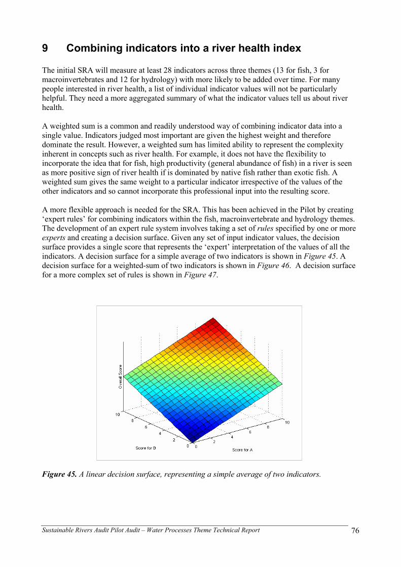
Sustainable Rivers Audit Pilot Audit – Water Processes Theme Technical Report
76
9 Combining indicators into a river health index The initial SRA will measure at least 28 indicators across three themes (13 for fish, 3 for macroinvertebrates and 12 for hydrology) with more likely to be added over time. For many people interested in river health, a list of individual indicator values will not be particularly helpful. They need a more aggregated summary of what the indicator values tell us about river health. A weighted sum is a common and readily understood way of combining indicator data into a single value. Indicators judged most important are given the highest weight and therefore dominate the result. However, a weighted sum has limited ability to represent the complexity inherent in concepts such as river health. For example, it does not have the flexibility to incorporate the idea that for fish, high productivity (general abundance of fish) in a river is seen as more positive sign of river health if is dominated by native fish rather than exotic fish. A weighted sum gives the same weight to a particular indicator irrespective of the values of the other indicators and so cannot incorporate this professional input into the resulting score. A more flexible approach is needed for the SRA. This has been achieved in the Pilot by creating ‘expert rules’ for combining indicators within the fish, macroinvertebrate and hydrology themes. The development of an expert rule system involves taking a set of rules specified by one or more experts and creating a decision surface. Given any set of input indicator values, the decision surface provides a single score that represents the ‘expert’ interpretation of the values of all the indicators. A decision surface for a simple average of two indicators is shown in Figure 45. A decision surface for a weighted-sum of two indicators is shown in Figure 46. A decision surface for a more complex set of rules is shown in Figure 47.
Figure 45. A linear decision surface, representing a simple average of two indicators.

Sustainable Rivers Audit Pilot Audit – Water Processes Theme Technical Report
77
Figure 46. A linear decision surface, representing a weighted sum of two indicators.
Figure 47. Example of a non-linear decision surface for two indicators4.
4 Note: the colours in Figures 45-47 are not intended to correspond to condition assessment map gradings presented in technical reports for other SRA themes.

Sustainable Rivers Audit Pilot Audit – Water Processes Theme Technical Report
78
The same principle applies for three or more indicators, but the surface is harder to display on paper. The use of an expert system allows for a broad range of decision surfaces that may include the simple weighted sum if this is what is considered to be the optimum way of combining the indicators. It can also produce an output which takes into account the interactions between different indicators (as in the example for fish above). The process of developing the decision surface for complex rules uses an area of mathematics known as fuzzy logic. The use of fuzzy logic ensures that a small change in the value of one indicator does not cause a sudden jump in the result (which is often the case if indicators are classed into categories). It also allows outputs to be generated when there is a degree of uncertainty (‘fuzziness’) about the inputs and their relationship to the output. This is a particularly important asset when there is uncertainty associated with measured values, or when river health is similar across a range of indicator values. An expert system documents the opinion of a particular set of ‘experts’ at a particular time. Conceptually, it is a similar process to expert panels, which have become popular in recent times for the same reasons (Swales and Harris, 1994; Thoms et al., 2000). However, the advantage of the expert system approach is that the rules and decisions are documented, transparent, repeatable, can be adjusted where necessary, and can be integrated. Expert rules may be modified over time as our understanding of river health increases. Provided the same indicators are involved, a new expert system can be applied retrospectively to earlier data and the results compared. Similarly, the affect of applying alternative expert systems which reflect competing opinions or concepts can be explored. Matlab, a powerful scientific and engineering computing software package used worldwide for technical computing, was used to develop expert systems for the SRA Pilot from the rules developed by experts involved in the process. The expert systems generated in the Pilot exist as computer software. They are menu-driven and can accept data either manually or from an Excel file. Data checking is included for quality control. Output can be provided as a file or on the screen. The software for any or all of the systems can be provided to others as needed to enable them to apply the system to their input data. The development of the expert system is done in four steps:
1. expert evaluation of the relationships between indicators and the need for/benefit of grouping them on the basis of similar roles or information content as they pertain to ecological condition and river health;
2. expert ranking of the river health output for each combination of input indicator values (eg high, medium, high; high, low, low etc), and converting the ranking into a score;
3. coding the rules within a software platform (e.g. Matlab), using the resulting decision surface to check that the rule sets accurately reproduce the above scores, and analysing dummy and real data to check results (with the experts);
4. finalising the rule set coding for later use in analysing data.
The details of all expert systems developed during the Pilot Sustainable Rivers Audit are documented in Carter (2003). A preliminary attempt was made to combine indicators into an overall river health index for water quality, assuming that all indicators would be included in the SRA program (step 1). These ‘expert rules’ were presented at the final technical workshop as an example of how indicators

Sustainable Rivers Audit Pilot Audit – Water Processes Theme Technical Report
79
could be combined, and the attempt was a useful exercise to put together a number of expert rules in a similar fashion as has been done for other themes. The steps involved included the assessment of criteria as presented in section 8, and the grouping of indicators according to information content. Sustainable Rivers Water Indexmetabolic (SR-WIm)5: Metabolic rate indicators: these indicators include GPP and R24 (measured over 24hr period), pelagic chlorophyll-a, and diurnal DO. Each of these provides some different information content on metabolic rates and changes relating to changes in surrounding land use. Metabolic rate indicators, Chlorophyll-a and diurnal DO also to be looked at together. Sustainable Rivers Water Indexnutrient (SR-WIn): ‘Nutrient’ driver indicators: Ortho-P, TP, TN, NOX, NH4 and C12:C13 and N14:N15 isotope ratios. Ratios of NOX:TN (degree of mineralisation) and NH4:NOX (oxidisation/reduction ratio), as proposed by the CRCFE Framework report (Whittington et al., 2001) could be considered in this category, although it is not clear how reference is set and what the information is telling us with regard to river health. Sustainable Rivers Water Indexphysical (SR- WIp): ‘Physico-chemical’ driver indicators: Temperature, Turbidity, pH, DO (% saturation) and Conductivity. The workshop participants decided that the scoring for reference condition between 0-1 was not adequate since it assumes a linear relationship between indicator change and river health condition. For many indicators this is not a valid assumption, and the relationship between each of the indicators and river health needs to be determined. The workshop participants also preferred using raw data for setting expert rules, as they provide more meaningful benchmarks than indicators on a scale from 0-1. A decision tree model as was set up for GPP could be refined and may include more indices than are currently included. It was felt that isotope ratios could not be included in the assessment of river health at this stage, as this indicator is still considered to be in a developmental stage. Clearly, the integration of indicators would require more work to be done and will depend on which components (if any) of the water processes theme will be included in the SRA at some point in the future.
5 The names of the indices were changed to remain consistent with name changes for other SRA themes. At the workshop, the index and (sub)indices were called River Health Water (X) or RHW(X).

Sustainable Rivers Audit Pilot Audit – Water Processes Theme Technical Report
80
10 Recommendations and Conclusions The result of a cost/benefit analysis of this theme (not explored in this document, see SRA design report) is that neither of the water processes components were advocated for inclusion in the first stage of implementation of the SRA. A further consideration was the substantial overlap of a potential water quality/process component of the SRA with existing State water quality monitoring programs. While these existing programs can provide useful information into the Auditing process (possibly to support or interpret assessments based on other indicators), it was not considered appropriate to attempt to make water quality assessments based on current State data programs meet the SRA objectives. Instead, this information can be used for interpretive purposes where this should be required. Recommendations for inclusion of components of the water processes theme during the first stage of the SRA are therefore limited to only three. The additional conclusions resulting from the Pilot study are listed under the proviso of the entire theme being included into the SRA at some point in the future.
10.1 Recommendations Recommendation 1: Remote sensing as a tool for water quality/processes assessment It is recommended that a Pilot study be undertaken (as recommended by the Remote Sensing Technical Scoping document, and adopted for the development of the SRA themes Floodplain, Physical Form and Riparian Vegetation) to assess the practical viability of remote sensing for water quality monitoring. This can be done in conjunction with method development for the other themes (physical form, riparian vegetation and floodplain assessment), and is seen as having potential because of the high cost of data collection for water quality spot measurements in the field. The study would aim to:
• scope the type and number of water quality variables that can be measured with remote sensing. Overseas use of RS techniques suggest potential for measuring GPP, R and chlorophyll-a
• determine its resolution, accuracy, cost and potential spatial and temporal coverage of streams in the Basin
• establish calibration methods for calibrating RS data with data collected in the field for field verification.
The Remote Sensing Technical Scoping study which was undertaken by CSIRO to investigate aspects of river health that could be assessed using remote sensing was mainly focussing on geomorphology and riparian vegetation, but has also identified the potential for some water quality aspects to be included in such assessment. The scoping study recommended a proposed Pilot Study to: ‘…broaden discussion on the utility of remote sensing for SRA assessment and to provide better estimates of the associated costs.’ ‘This exercise would further identify the optimal sensor suite as a complement to the current ground-based riparian health assessments. It would also assist in development of more customised field sampling protocols.’ (Environmental Remote Sensing Group, 2003). The potential of using of telemetry (real time data-loggers) should also be investigated further with regard to spatial deployment capabilities, cost/benefit return compared to other methods, reliability of data collection and confidence levels.
Sustainable Rivers Audit Pilot Audit – Water Processes Theme Technical Report
81
This technology was not explored in the Pilot project, but ISRAG suggested that it should be further explored as an option for cost effective data collection on water processes. It could be used in conjunction with remote sensing to validate RS data in the field. Recommendation 2: developing guidelines It is recommended that ISRAG develops guidelines for the collection, integration and interpretation of water quality data collected under a variety of (State) programs in order to assist with the assessment of river health and the interpretation of results collected under the SRA program. This could include nutrient budget models, developed under the National Land and Water Resources Audit by Young et al. (2001) and Prosser et al. (2001), and equilibrium models developed by the CRCFE (Lawrence, 2002). By doing so, best use is made of existing water quality monitoring programs. The guidelines would need to cover:
• quality control/quality assurance of the data collected by the State agencies
• defining limits, possible bias and differences between those programs and the SRA (sample design, spatial and temporal distribution of sites, etc)
• defining resolution, data gaps and comparability of results between programs
• developing guidelines on how data interpretation will be done to make it an open and transparent process.
Water quality data to be collected as part of macroinvertebrate and fish sampling could also be used as an interpretive aid using the guidelines developed by ISRAG. Their value is limited due to the limited frequency but these data can be collected at minimal extra cost. Recommendation 3: Metabolic processes (GPP/R24) It is recommended that the SRA keep a watching brief over research related to metabolic processes and the development of GPP/R24 indicators as a routine monitoring tool. They have the greatest value in increasing our understanding the in-stream ecology, but due to our limited understanding at present no protocols exist for routine monitoring. The whole-stream method shows the greatest potential for developing a routine monitoring tool, despite the inaccuracies with determining re-aeration coefficients. It is the preferred method due to the following problems with the use of chamber methods as a routine monitoring tool:
• Monitoring equipment is complex, requires specialist training, high intensity maintenance and is prone to high failure and damage
• Metabolic rate measurements are not integrating rates at the reach level, and cannot be compared between upland and lowland areas
• Establishing reference condition would require extensive work
• Measurements are habitat specific (ie of no cobbles available nothing can be measured. Further exploration of conceptual models and existing datasets will be required to refine the reference conditions for Gross Primary Production and Respiration which were developed during the Pilot study. The watching brief could include developments regarding organic material (DOC, TOC, FPOM, CPOM) as additional process indicators. ISRAG has indicated in their ‘Response to the SRA Business Case’ that they are interested in including the metabolic processes component into the SRA program at some point in the future.
Sustainable Rivers Audit Pilot Audit – Water Processes Theme Technical Report
82
Regular monitoring of in-stream metabolic rates shows greatest potential in increasing our understanding of in-stream ecological processes, and is information currently not collected by State jurisdictions. Whilst the SRA recognises that further method development would be required before these indicators could be included in a routine monitoring program, it was felt that completing further research was outside the scope of the SRA objectives.
10.2 Conclusions The conclusions listed below are the result of work undertaken during the Pilot. They are currently constrained by the low cost/benefit return and possible duplication of data collection programs, and are hence not formulated as recommendations. It is conceivable that at some point in the future the need for inclusion of a water processes theme in the SRA will be reconsidered, in which case these conclusions drawn from the Pilot will still be valuable.
10.2.1 Water column physico-chemical characteristics and chlorophyll-a Indicator selection In the event of the water processes theme being included in the SRA it is recommended to assess water quality river health at the valley scale, using the indicators that were assessed during the Pilot study. The assessment would provide a ‘snapshot’ of river health for each year during the season of base-flow, and would be an indication of the resilience of the system. The same sites would be sampled that are used for macroinvertebrate sampling, but sampling would occur at different times of the year. Spot measures of physico-chemical indicators can have interpretive value for several of the SRA themes, including the water process theme. Physico-chemical indicators of water quality characteristics can be seen as ‘drivers’ influencing important ecological processes. However they do not aid the quantification of river processes on the broad temporal and spatial scales proposed by the SRA. Water quality can also be regarded as an outcome of health in its own right, a resulting sum total of water inputs, flow and in-stream ecological processes, and as a habitat medium for many organisms. Ideally these indicators should form part of the SRA program, but their role in river health assessment should be made explicit and be distinguished from other water quality objectives. Reference condition In the event of the water processes theme being included in the SRA it is recommended that for spot measurements (physico-chemical indicators) 20th and 80th percentile boundaries are determined for all SRA valleys, based on existing datasets6. This would require mining data from various water quality monitoring programs and is part of further method development for water quality sampling. Since reference condition would be determined for base-flow conditions only, temporal stratification is not envisaged. Defining reference condition for the proposed sampling window would need to be determined before the first assessment of river health condition could be conducted. This would need to be done for all Basin valleys, and would require a coordinated approach. Reporting against targets and for long term trend detection would gain importance over time and gradually replace assessment against reference condition.
6 For Victoria, SEPP values could be used. They are 25th and 75th percentiles and are based on bioregions. A uniform approach (using 20th and 80th percentiles) throughout the Basin would require recalculating percentiles from the raw data of existing datasets.

Sustainable Rivers Audit Pilot Audit – Water Processes Theme Technical Report
83
Number of sites and sampling frequency In the event of the water processes theme being included in the SRA it is recommended that the same sites would be sampled as those sites selected for macroinvertebrate sampling, 35 per river valley. This would result in a confidence level similar to that established for macroinvertebrates for the average of all indicators, and amounts to the ability to detect a 10% change with a confidence level of α = 0.05 and a power of 0.8 at the valley scale. Post-hoc power analysis would need to be conducted to determine confidence levels for each of the indicators separately, as it is not possible to determine site numbers for each indicator separately. Over time, the power to detect change will increase and will enable trend analysis. The recommended sampling frequency would be 6 times annually during base-flow conditions, to enable trend detection from year to year. Post-hoc power analysis will be required to establish the power level of detection of change, taking into account accumulation of data over time.
10.2.2 Stable N and C isotope ratios as indicators of river health In the event of the water processes theme being included in the SRA it is recommended that the value of these indicators for river health be further explored. Routine monitoring protocols exist for data collection and analysis, and the use of isotope ratios may increase our understanding of in-stream processes and modifiers. There appears to be a strong correlation between surrounding land use and N isotope signatures, but the exact causal relationship of this correlation has not been established. This indicator would potentially be useful in establishing the relationship between the function of riparian vegetation as a buffer between impacts resulting from modified land use in the surrounding catchment. The C isotope ratios could potentially be used as an indicator of groundwater interactions, but further research - outside the scope of the SRA - is required to establish if confounding factors in the isotope signature could be interpreted. C isotopes can also be used as a check on extreme values of GPP, and may be a useful aid in developing methods for accurate GPP measurement. The collection of primary consumers has the potential for integrating these indicators over different time scales. Collection and analysis of the data can be done at low cost, but training is required to ensure quality assurance of the data collected in the field. Reference condition The current recommendation from Bunn and Fellows (2003) for the upper limit for δ15N isotopes is in agreement with Ford (2003) and this could be adopted for use in a routine monitoring program. The usefulness of a reference condition for the lower limit of δ15N isotopes may need to be further explored, as well as the spatial area of surrounding land use represented by the test/reference sample. The use of this information could be optimised by matching it with land-use data, to explore the relationship and possibly further refine reference condition. Similar research is required for δ13 C isotopes, but this is outside the scope of the SRA program. Material to be collected and number of samples required Only algal material should be collected from all sites where this is available and vascular plant material should be excluded in order to meet the analysis requirement of full submergence. Collecting filamentous algae (and possibly primary consumers) would require the following QA/QC issues to be addressed: training, protocol revision and data recording. The collection of primary consumers could be trialled on a small scale by macroinvertebrate sampling teams, and the time spent collecting and preserving animals live (cold or frozen storage) for laboratory analysis should be recorded to determine the cost component of collecting this additional data. The power analysis indicates that 35 sites per valley is more than the number of sites required to detect a change of 0.1 at the valley level, so this number should be adequate even if material is not available from each site. The data would be analysed for δ15N, and results for δ13C could be used to check GPP measurements.

Sustainable Rivers Audit Pilot Audit – Water Processes Theme Technical Report
84
10.2.3 Sampling and analytical techniques Kjehldahl versus alkaline persulfate method for TP The alkaline persulfate method is suitable for determining TP loads for all samples <150 mg/L of SS. For samples with higher suspended solids alkaline persulfate is still the preferred method for standardisation purposes, despite the higher fractionation of phosphorus not biologically available. Chlorophyll-a calibration For an assessment on a Basin-wide scale it is possible that more than one laboratory would be used to analyse results. In order to get the most accurate results and achieve parity between laboratories, it is recommended to refine the protocols, to include chlorophyll-a analytical specifications as follows:
• the degradation products of chlorophyll-a to be determined (Chlorophyll-a and Phaeophytin-a), by spectrophotometry or fluorometry, depending on expected value range and with both methods being calibrated against each other.
• the degree of error associated with each method and with the Chlorophyll-a calibration standard
• standardisation of analytical methods, including calibration and analytical equipment Turbidity calibration To overcome variability in equipment sensitivity and sampling settling, it is recommended to measure turbidity in the field with data loggers. The equipment would need to be calibrated each time before undertaking a sampling run, and a number of replicate measurements should be taken at each site, to verify robustness of readings. The last reading would be recorded together with other variables (T, pH, conductivity, DO) being recorded simultaneously.

Sustainable Rivers Audit Pilot Audit – Water Processes Theme Technical Report
85
References ANZECC & ARMCANZ (2000). Australian and New Zealand Guidelines forFresh and Marine Water Quality. National Water Quality Management Strategy Paper No.4. Australian and New Zealand Environment and Conservation Council & Agriculture and Resource Management Council of Australia and New Zealand, Canberra. Bunn, S.E. and Fellows, C.S. (2003). Report on Stable Isotope Indicators. Report to the Murray Darling Basin Commission. Boon, P.I. & Bunn, S.E. (1994). Variations in the stable-isotope composition of aquatic plants and their implication for food-web analysis. Aquatic Botany 48: 99-108. Bunn, S.E., Davies, P.M and Winning, M. (2003). Sources of organic carbon supporting the food web of an arid zone floodplain river. Freshwater Biology 48: 619-635. Bormans, M. (2003). Assessment of reference values for water quality indicators: Chlorophyll-a, Gross Primary Production and Respiration in the SRA Pilot Monitoring Program. Final report to MDBC. Bunn, S.E., Davies, P.M., and Mosisch, T.D. (1999). Ecosystem measures of river health and their response to riparian and catchment degradation. Freshwater Biology 41: 333-345. Carter, S. (2003). Sustainable Rivers Audit Data Aggregation Software. Report to the Murray-Darling Basin Commission. Environmental Dynamics Project ED5090. Chessman, B., Growns, I., Currey, J. and Plunkett-Cole, N. (1999). Predicting diatom communities at the genus level for the rapid biological assessment of rivers. Freshwater Biology 41: 317-331. Cullen P., Harris, J. Hillman, T. Liston, P. Norris, R. and Whittington, J.(2000). Scope of the sustainable Rivers Audit. MDBC &CRCFE. Report. MDBC (2000). Review of the Operation of the Cap. Overview report of the Murray Darling Basin Commission Environmental Remote Sensing Group (2003). Determination of SRA Habitat Indicators by Remote Sensing. Technical Scoping document, CSIRO Land and Water. EPA Victoria (2003). State Environment Protection Policy - Waters of Victoria. Government Gazette No. S 107. Ford, P. (2003). Potential for the use of the isotopic ratios of Carbon and Nitrogen in the SRA Monitoring Program. Final report to MDBC. Grace, M.R. and Harper, M.P. (2003). A Modelmaker 3.0 program to extract metabolic parameters from diel oxygen curves. Monash University.

Sustainable Rivers Audit Pilot Audit – Water Processes Theme Technical Report
86
Growns, I.O.(1992). Macroinvertebrate Community Structure in the Streams of the Southern Forests of Western Australia: The influence of Seasonality, Longitudinal gradients and Forestry Activities. PhD Thesis, Murdoch University, WA. Growns, J.E, Chessman, B.C., McEvoy, P.K. and Wright, I.A. (1995). Rapid assessment of rivers using macroinvertebrates: case studies in the Nepean River and Blue mountains, NSW. Australian Journal of Ecology 20: 130-141. Hebert, C.E. and Wassenaar, L.I. (2002). Stable nitrogen isotopes in waterfowl feathers reflect agricultural land use in western Canada. Environmental Science and Technology 35, 3483-3487. Karr, J.R. (1991). Biological integrity: A long-neglected aspect of water resource management. Ecological Applications 1: 66-84. Ladson, A.R., White, L.J., Doolan, J.A.,Finlayson, B.L., Hart, B.T., Lake, P.S. and Tilleard, J.W. (1999). Development and testing of an Index of stream condition for waterway management in Australia. Freshwater Biology 41: 453-468. Lawrence, I. (2002). CRCFE River Assessment Tools. Models and description. Unpublished report. McNeil, V.H, Churchill, R.C., Marshall, C.J. and Choy, S.C (2000). Preliminary Risk Assessment of Water Quality in Queensland River Basins. Department of Natural Resources, Queensland.
McNeil, V., McNeil, A., Poplawski, W., and Zannakis, G. (1991). Basin 4223: The Upper Condamine Catchment. Desing of Water Quality Monitoring Network, Vol 1. Main Report, Water Resources Commission, Water Resource Assessment Division, Data Quality Control Section.
Norris, R.H. and Norris, K.R. (1995). The need for biological assessment of water quality: Australian perspective. Australian Journal of Ecology 20: 1-6. Norris, R.H. and Thoms, M.C. (1999). What is river health? Freshwater Biology 41: 197-209. Norris, R.H., Liston, P., Davies, N., Coysh, J., Dyer, F., Linke, S., Prosser, I. and Young, W. (2001). Snapshot of the Murray-Darling Basin River Condition. Report to the Murray-Darling Basin Commission. Poirier, D., Potts, J. and Carpenter, M. (2003). Water Column and Benthic Metabolism: Review of the Concepts and Methods for Monitoring for the Murray Darling Basin Sustainable Rivers Audit (MDBSRA). NSW EPA report. Prosser, I.P., Rustomji, P., Young, W.J., Moran, C.J. and Hughes, A.O. (2001) Constructing River Basin Sediment Budgets for the National Land and Water Resources Audit. Technical Report 15/01, CSIRO Land and Water, Canberra. Reid, M.A., Tibby, J.C., Penny, D. and Gell, P.A. (1995). The use of diatoms to assess past and present water quality. Australian Journal of Ecology 20: 57-64. Resh, V.H., Norris, R.H. and Barbour, M.T. (1995). Design and implementation of rapid assessment approaches for water resource monitoring using benthic macroinvertebrates. Australian Journal of Ecology 20: 108-121.

Sustainable Rivers Audit Pilot Audit – Water Processes Theme Technical Report
87
Robinson D.P., Rooney G.R., and Jirik S. (1994). Temporal Trends Analysis of Data from the Water Quality monitoring network, 1984-89. Environment Protection Authority, Victoria, Australia. Publication no. 430. Simpson, J., Norris, R., Barmuta, L. and Blackman, P. (1996). Australian River Assesment System: National River Health Program Predictive Model manual. URL http://ausrivas.canberra.edu.au/ausrivas. Smith, M.J. and Storey, A.W.(Ed) (2001). South East Queensland Regional Water Quality Management Strategy. Stage 3. Project DIBM3: Design and Implementation of baseline monitoring. Final Report. Swales, S. and Harris, J.H. (1994). The Expert Panel Assessment Method (EPAM): A New Tool for Determining Environmental Flows in Regulated Rivers. In: The Ecological Basis for River Management (Eds. D. Harper and A. Ferguson,) pp.125 - 134. John Wiley and Sons, Chichester. Thoms, M., Suter, P., Roberts, J., Koehn, J., Jones, G., Hillman, T., and Close, A. (2000). River Murray – Dartmouth toWellington and the Lower Darling River. Report of the River Murray Scientific Panel on Environmental Flows. Thorp, J.H. and Delong, M.D.(1994). The riverine productivity model: an heuristic view of carbon sources and organics processing in large river ecosystems. Oikos 70: 305-308 Udy, J.W. and Bunn, S.E. (2001). Elevated δ15N values of aquatic plants in cleared catchments: why? Marine and Freshwater Research 52, 347-351. Vannote, R.L., Minshall, G. Cummins, K.W., Sedell, J.R and Cushing, C.E.(1980) The River Continuum Concept. Canadian Journal Fisheries and Aquatic Sciences 37: 130-137 Whittington, J., Coysh, J., Davies, P., Dyer, F., Gawne, B., Lawrence, I., Liston, P., Norris, R., Robinson, W. and Thoms, M.(2001) Development of a Framework for the Sustainable Rivers Audit. Technical Report #7/2001, Cooperative Research Centre for Freshwater Ecology. Whitton, B.A. and Kelly, M.G. (1995) Use of algae and other plants to assess past and present water quality. Australian Journal of Ecology 20: 45-56.
Wright, I.A., Chessman, B.C., Fairweather, P.G. and Benson, L.J. (1995). Measuring the impact of sewage effluent on the macroinvertebrate community of an upland stream: The effect of different levels of taxonomic resolution and quantification. Australian Journal of Ecology 20: 142-149. Young, W.J., Chessman, B, Erskine, W., Jaleman, A, Raadik, T., Tilleard, J., Valey, I., Wimbush, D and Verhoeven, J. (1988). Environmental assessment method for the rivers in the area of interest of the Snowy Water Inquiry. In: anon.(1988) Resource materials – Appendix to the final report of the Snowy Water Inquiry, 44pp. (http://www.snowywaterinquiry.org.au/documents/appendix/appendix.htm)

Sustainable Rivers Audit Pilot Audit - Water Processes Theme Technical Report - Appendices 88
Appendices
APPENDIX 1 Workshop and technical group participants a: Workshop participants initial workshop 10-11 April 2002 First Name Last Name Organisation Email Myriam Bormans CSIRO Land and Water [email protected] Heather Hunter QLD DNRM [email protected] Bernard Prendergast BRS [email protected] Bruce Chessman NSW DIPNR [email protected] Greg Raisin NSW [email protected] Helen Daly NSW [email protected] Kylee Wilton DIPNR [email protected] Brian Bycroft QLD DNRM [email protected] John Bennett QLD EPA [email protected] Geoff Coade NSW EPA [email protected] Klaus Koop NSW EPA [email protected] Peter Scanes NSW EPA [email protected] Eren Turak NSW EPA [email protected] Gary Bickford MDBC (no longer with MDBC) Christie Fellows Griffith University [email protected] Alieta Donald VIC [email protected] David Duncan SA [email protected] Ian Lawrence CRCFE [email protected] Barry Hart Monash University [email protected] Terry Hillman ISRAG [email protected] Peter Davies ISRAG [email protected]
b: List of members of the reference reconstruction group First Name Last Name Organisation Email Myriam Bormans CSIRO Land and Water [email protected] Justin Brooks CRCWQT [email protected] Geoff Coade NSW EPA [email protected] Heather Hunter QLD DNRM [email protected] Leon Metzeling VIC EPA [email protected] Peter Davies UWA [email protected] Jody Swirepik MDBC [email protected] Frederick Bouckaert MDBC [email protected] Julie Coysh MDBC [email protected] Wayne Robinson MDBC [email protected]
c: Workshop participants final workshop 21 July 2003 First Name Last Name Organisation Email Myriam Bormans CSIRO Land and Water [email protected] Justin Brooks SA Aust Water Quality Centre [email protected] Geoff Coade NSW EPA [email protected] Heather Hunter QLD DNRM [email protected] David Robinson VIC EPA [email protected] Peter Davies UWA [email protected] Jody Swirepik MDBC [email protected] Frederick Bouckaert MDBC [email protected] Andrew Moss QLD EPA [email protected] Sarah Johnston EA [email protected] Bruce Cooper NSW DIPNR [email protected] Stuart Bunn Griffith University [email protected]

APP
EN
DIX
2: G
IS m
ap o
f all
NR
HM
P sa
mpl
ing
site
s situ
ated
with
in th
e Pi
lot v
alle
ys fo
r w
hich
wat
er q
ualit
y da
ta
wer
e us
ed in
det
erm
inin
g re
fere
nce
cond
ition
(cal
cula
tion
of 2
0th a
nd 8
0th p
erce
ntile
s)
Sustainable Rivers Audit Pilot Audit - Water Processes Theme Technical Report - Appendices 89

Sustainable Rivers Audit Pilot Audit - Water Processes Theme Technical Report - Appendices
90
APPENDIX 3: Pilot sampling protocols
Murray-Darling Basin Commission
Sustainable Rivers Audit
Pilot Audit
Program
Water Processes Sampling Protocol
PART B
DRAFT
Version of 11 September 2002∗
∗ Tables and Figures were renumbered to distinguish from Table/Figure numbering in main body of technical report; Appendices are renamed Annexes.

Sustainable Rivers Audit Pilot Audit - Water Processes Theme Technical Report - Appendices
91
Appendix 3 Table of Contents
1 Objectives of the manual ............................................................................................... 92
2 Sites ..................................................................................................................................... 92 2.1 Reference condition and Types of sites ........................................................................ 92 2.2 Number of sites - introduction ...................................................................................... 92 2.3 Number and location of assessment sites...................................................................... 93 2.4 Number and site selection process for best available sites ........................................... 93 2.5 Length of sites............................................................................................................... 95
3 Sampling frequency season and conditions at sites ......................................................... 95 3.1 Sampling frequency and season.................................................................................... 95 3.2 Sampling / Site Conditions ........................................................................................... 96
Cheat sheet: Water processes sampling design summary.............................................. 97
4 Description of indicators ............................................................................................... 98
5 Rationale for selection of process indicators .................................................................... 99
6 Description of sampling and analytical methods ........................................................... 100 6.1 Use of Standard Methods............................................................................................ 100 6.2 Replicates for bottle samples ...................................................................................... 100 6.3 Rate Measurements ..................................................................................................... 100 6.4 Spot Measures - Standing Stocks................................................................................ 104
7 Skill requirements, training and OH&S......................................................................... 112
8 QA/QC and Data Management .................................................................................... 112
9 References APPENDIX 3 .............................................................................................. 113

Sustainable Rivers Audit Pilot Audit - Water Processes Theme Technical Report - Appendices
92
1 Objectives of the manual This protocol manual explains the sampling protocols that will be trialed to sample the water processes component of river health across four pilot valleys in the Murray-Darling Basin. This is a working document for use in the Pilot Audit and it is anticipated that the protocols contained within will be revised after the Pilot Audit. It is intended that participating governments will use these protocols to draw up a sampling/operational manual specific to their pilot valley by adding information on sites chosen, access, etc.
2 Sites
2.1 Reference condition and Types of sites Sampling for the water processes component of the Pilot Audit will be at both “assessment” sites and a small number of “best available” sites. “Assessment” sites will form the basis of the health assessments of the Pilot valley whereas best available sites will inform the construction of reference condition (natural has been adopted as reference for the Pilot Audit) which helps in the interpretation of observations at the assessment sites. Use of data from best available sites will only be one source of information for a project that will define reference condition (project summarised in Figure below from Water Quality Workshop in Melbourne April 2002).
2.2 Number of sites - introduction The number of sites required for the SRA will depend on the:
• spatial reporting scale of the assessment, • variability of the indicator, • initial condition score of the indicator, • aggregation and reporting statistics used, • desired level of change to be detected, and • desired confidence in detecting that change.
CONCEPTUAL
Existing data and models
Numerical models
Range of river/channel type
Range of disturbances
Some best available site data
Requested from pilot data
Ref
condition group

Sustainable Rivers Audit Pilot Audit - Water Processes Theme Technical Report - Appendices
93
2.3 Number and location of assessment sites The number of assessment sites for the Pilot Audit has been chosen with various considerations across the themes. One of the objectives of the Pilot is to provide data to determine the appropriate “effect size” and hence sample size for the full SRA. Power analyses have informed the decision of the number of pilot sites, particularly for the fish and macroinvertebrate themes, but practical issues (time and costs) also need to be considered. Another important issue is parity in site locations across themes. Collecting the most informative selection of data has led to the decision to have as much site overlap as possible between themes – at least for the Pilot Audit. The hydrology, physical habitat and water quality themes are also intended to assist with the interpretation of the biotic indicators so in general it will be useful to have this information at as many sites as possible where macroinvertebrates or fish are sampled. Taking these issues into consideration, it has been agreed that sampling for the assessment of water processes should occur at the fish assessment sites, giving a total number of approximately 20 assessment sites per Pilot Catchment. The method used for selection of fish assessment sites is at Appendix A (for information only);- there is no need for reselection of sites using these methods for the water processes theme.
2.4 Number and site selection process for best available sites The construction of reference condition will be done by an expert group (nominated at the Melbourne Workshop) who may use information from any of the following sources to determine the range of expected natural conditions for each VPZ:
• Data from best available sites • Historical data/observations • Data from sites other than specially selected best available sites • Conceptual or numerical modelling • Literature and expert knowledge. The aim of using this process to “construct” natural is to overcome the problem of there not being sites which can be accepted as being in natural condition (this is especially true in lowland areas). For the water processes theme, it is expected that the majority of the construction of reference will be based on expert knowledge and existing data, hence only a few “best available” sites are being sampled. Up to 11 best available sites can be selected for sampling in the Pilot Audit. These eleven sites should be broken up across the VPZs – preferably in a manner which reflects the break-up of assessment sites (which were based on catchment area giving more sites in the lowland regions). A notional break-up between the 3 VPZs is 3 in source, 3 in transportational and 5 in depositional. Best available sites should be selected by identifying potential good quality sites (using existing datasets or local knowledge) and then ranking these potential sites using the matrix in the table below. When this system is used, the lower scoring sites are the ‘best available’ sites. Note that the disturbance and influence categories in this table are the same used to evaluate the best available fish sites and only the weightings have been changed. Thus sites evaluated for the fish theme should be easily evaluated as potential sites for this theme by recalculating the ranking based on the new weightings. States may choose to use the best available macroinvertebrate and fish sites (where sites are in the Pilot catchment) as input to this ranking process to minimise the workload.

Sustainable Rivers Audit Pilot Audit - Water Processes Theme Technical Report - Appendices
94
Table A3-1. Rating system for assessing human disturbance at potential reference/best available water process sites
Disturbance High influence = 3 Medium influence = 2 Low influence = 1 [Manufacturing] Industry includes factories, mining, power plants Weighting = 3
Industrial areas adjacent to the site or close upstream (< about 20km); industrial discharges enter the stream
Substantial industrial areas in the catchment but not close to the site
No industrial areas in catchment (small catchments) or industrial areas remote from the site and a minuscule proportion of catchment area (large catchments)
Urbanization Weighting = 3
Site lies within or close downstream of high-density urban area; urban drainage or sewage discharge enters the stream
Substantial urban areas in the catchment but not close to the site; or low-density urban areas only near the site, without direct drainage or discharge
No urban areas in catchment (small catchments) or urban areas remote from the site and a minuscule proportion of catchment area (large catchments)
Irrigated Cropping Weighting = 3
Large irrigated cropping areas (e.g. horticulture, cotton, rice farms) adjacent to the site or close upstream; tailwater drainage enters the stream
Substantial cropping areas in the catchment but not close to the site
No cropping in catchment (small catchments) or cropping remote from the site and a minuscule proportion of catchment area (large catchments)
Dryland cropping / riparian Weighting = 1
Large dryland cropping areas (e.g. wheat, oilseeds farms) adjacent to the site or close upstream;
Substantial dryland cropping areas in the catchment but not close to the site
No dryland cropping in catchment (small catchments) or cropping remote from the site and a minuscule proportion of catchment area (large catchments
Grazing / riparian Weighting = 2
Riparian zone intensively grazed; faeces, pug-marks, eroded access tracks, or chewing down of vegetation conspicuously present
Riparian zone ungrazed or lightly grazed, but substantial riparian grazing near site, close upstream or through much of catchment
No grazing in catchment (small catchments) or grazing areas remote from the site and a small proportion of catchment area (large catchments)
Recreation Weighting = 0
Clear evidence of recreational use, e.g. people present, trampling, litter, fishing lines
No clear evidence of recreation but accessibility suggests some use is likely
Site unlikely to be accessed for recreation
Water extraction Weighting = 2
Large irrigation districts upstream of the site; total flow volume greatly reduced
Only localised irrigation upstream of the site; total flow volume not greatly reduced but substantial portion of low flow may be extracted
Little or no extractive use upstream of the site
Flow regulation Weighting = 2
Seasonal or diel pattern of flows greatly altered by upstream storage and release patterns
Upstream impoundment alters diel or seasonal flow pattern, but unregulated tributary flows result in substantial normalization
No significant upstream impoundment
Hypolimnetic release Weighting = 3
Bottom-release dam <150km upstream; summer temperatures substantially below natural; winter temperatures may be elevated
Bottom-release dam upstream but >150km distant from site; seasonal temperature regime only moderately altered
No significant upstream impoundment or upstream impoundment with effective multi-level offtake

Sustainable Rivers Audit Pilot Audit - Water Processes Theme Technical Report - Appendices
95
Artificial barriers Weighting = 1
High barriers <150km downstream of the site, likely to be severely constraining fish migration
Barriers are likely to be affecting migration to/from the site but they are low or distant from the site
Any barriers are upstream and remote from the site.
Alien fish Weighting = 1
Alien fish dominate the site in terms of either numbers or biomass
Alien fish present but do not dominate
No alien fish at the site
Alien plants Weighting = 0
Riparian zone has lost most or all of original tree and shrub cover; riparian and aquatic vegetation dominated by alien species
Riparian zone retains native trees and shrubs but substantial alien vegetation present. Aquatic plants predominantly native
Riparian and aquatic vegetation not cleared. Little or no alien plant invasion
Geomorphic change Weighting = 1
Poor geomorphic condition (River Styles™ or similar method)
Moderate geomorphic condition (River Styles™ or similar method)
Good geomorphic condition (River Styles™ or similar method)
Note: these are currently exactly the same categories used for the fish process but with different weightings.
The process for selection of potential best available sites should identify more sites than can actually be sampled so that if a site cannot be sampled then you can proceed to the next one on the list.
2.5 Length of sites • The size of a site for the purposes of sampling water processes was not defined at the
Melbourne workshop. • For macroinvertebrates, the size of a site is generally the full width of the stream and 10
times the full width in length. • For fish sampling, the size of a site is up to 1km long
Sampling for the water processes theme does not require a large area since there are few area based requirements in the methods. The sampling for water quality/process should occur, where possible, at the location that the macroinvertebrate monitoring was undertaken with a maximum area used reflecting the size of the macroinvertebrate sampling site. If this location is unsuitable for the rate-measuring work because of deployment requirements or equipment security issues, the second approach would be to use any location within the fish-sampling site.
3 Sampling frequency season and conditions at sites
3.1 Sampling frequency and season • All States should sample each site only once in each of three seasons:- winter 2002, spring
2002 (to be done during macroinvertebrate sampling where possible) and high summer 2003 (Table A3-2). Samples should be collected for primary and secondary process indicators (viz. plant material for delta C and delta N, pelagic chlorophyll-a, nutrients (N&P) and turbidity).
• All States should measure whole stream diel DO/pH/temperature at a sub-selection of sites in winter and summer (not spring) (Table A3-2). This should be done at approximately 10 sites across the pool of assessment and best available sites. NSW will do this at the locations that they do benthic/pelagic GPP monitoring. . These sites should be “secure” meaning little likelihood of equipment being removed or tampered with if left unattended.
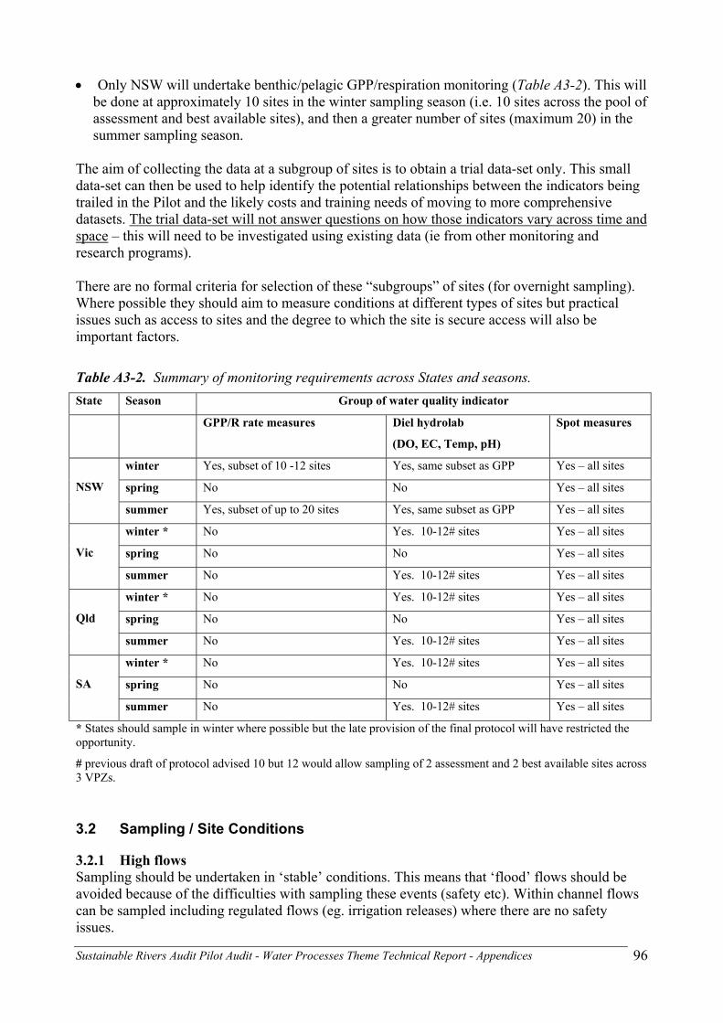
Sustainable Rivers Audit Pilot Audit - Water Processes Theme Technical Report - Appendices
96
• Only NSW will undertake benthic/pelagic GPP/respiration monitoring (Table A3-2). This will be done at approximately 10 sites in the winter sampling season (i.e. 10 sites across the pool of assessment and best available sites), and then a greater number of sites (maximum 20) in the summer sampling season.
The aim of collecting the data at a subgroup of sites is to obtain a trial data-set only. This small data-set can then be used to help identify the potential relationships between the indicators being trailed in the Pilot and the likely costs and training needs of moving to more comprehensive datasets. The trial data-set will not answer questions on how those indicators vary across time and space – this will need to be investigated using existing data (ie from other monitoring and research programs). There are no formal criteria for selection of these “subgroups” of sites (for overnight sampling). Where possible they should aim to measure conditions at different types of sites but practical issues such as access to sites and the degree to which the site is secure access will also be important factors.
Table A3-2. Summary of monitoring requirements across States and seasons. State Season Group of water quality indicator
GPP/R rate measures Diel hydrolab
(DO, EC, Temp, pH)
Spot measures
winter Yes, subset of 10 -12 sites Yes, same subset as GPP Yes – all sites
spring No No Yes – all sites
NSW
summer Yes, subset of up to 20 sites Yes, same subset as GPP Yes – all sites
winter * No Yes. 10-12# sites Yes – all sites
spring No No Yes – all sites
Vic
summer No Yes. 10-12# sites Yes – all sites
winter * No Yes. 10-12# sites Yes – all sites
spring No No Yes – all sites
Qld
summer No Yes. 10-12# sites Yes – all sites
winter * No Yes. 10-12# sites Yes – all sites
spring No No Yes – all sites
SA
summer No Yes. 10-12# sites Yes – all sites
* States should sample in winter where possible but the late provision of the final protocol will have restricted the opportunity.
# previous draft of protocol advised 10 but 12 would allow sampling of 2 assessment and 2 best available sites across 3 VPZs.
3.2 Sampling / Site Conditions
3.2.1 High flows Sampling should be undertaken in ‘stable’ conditions. This means that ‘flood’ flows should be avoided because of the difficulties with sampling these events (safety etc). Within channel flows can be sampled including regulated flows (eg. irrigation releases) where there are no safety issues.

Sustainable Rivers Audit Pilot Audit - Water Processes Theme Technical Report - Appendices
97
3.2.2 Dry sites Assessment sites
Where a selected assessment site is dry (note these sites are the same sites as the fish assessment ones), then record this and generally do not replace with another site unless a minimum number of sites cannot be sampled. This minimum is 3 sites in each of source and transport VPZs, and 5 sites in depositional VPZ. If replacement of assessment sites is needed to reach the minimum, sample at macroinvertebrate assessment sites in preference to selecting new sites. In this case “dry” would mean that you couldn’t find a zone as big as a macroinvertebrate site (see size of sites) within the 1 km of the defined fish site. Best Available sites The process for selection of potential best available sites should identify more sites than can actually be sampled so that if a site cannot be sampled then the next best quality site on the list can be sampled instead.
Cheat sheet: Water processes sampling design summary The following is a brief summary of the above text – please go back to the text for more detailed information:
Assessment Sites: • Approximately 20 assessment sites at the same location as fish sites. • Field operators can choose to collect indicators listed as spot measures at macroinvertebrate
sites that are on the direct route to a fish site (=opportunistic sampling). This can be done at a maximum of 3 sites (aim is to boost the dataset with little extra cost).
• Where fish assessment sites are dry, then generally do not replace with other sites unless unable to get a minimum number of assessment sites being 3 sites in each of source and transport VPZs and 5 sites in depositional VPZ.
• If replacement of assessment sites is needed to reach the minimum, then sample at macroinvertebrate assessment sites in preference to selecting new sites.
Best Available sites: • Up to 11 sites can be sampled to contribute information to the construction of reference
condition (but this will only be one data source for this procedure). • These 11 sites should notionally be spread 3, 3, and 5 across source, transport and
depositional VPZs. • Fish, and where they exist, macroinvertebrate “reference” sites should be assessed as
preferable water process best available sites.
Collection of types of indicators across States/sites/season. • All States should sample each site only once in each of three seasons:- winter 2002, spring
2002 (to be done during macroinvertebrate sampling where possible) and high summer 2003. Samples should be collected for primary and secondary process indicators listed as spot measures in the methods section of this appendix (viz. plant material for delta C and delta N, pelagic chlorophyll-a, nutrients (N&P), turbidity, clarity, electrical conductivity, pH (spot measure) alkalinity and flow).
• All States should measure whole stream diel DO/pH/temperature (and where possible EC) at a sub-selection of sites in winter and summer (not spring). This should be done at approximately 10 -12 sites across the pool of assessment and best available sites. NSW will do this at the locations that they do benthic/pelagic GPP monitoring.

Sustainable Rivers Audit Pilot Audit - Water Processes Theme Technical Report - Appendices
98
• Only NSW will do benthic/pelagic GPP/respiration monitoring. This will be done at approximately 10 sites in the winter sampling season (ie. 10 sites across the pool of assessment and best available sites), and then a greater number of sites (maximum 20) in the summer sampling season.
4 Description of indicators Table A3-3 provides a list of indicators that will be trialled in the Pilot SRA for the Water Processes theme. (Note that the text in the right column needs further work). The process of choosing water quality indicators for the SRA grouped indicators into ecological process indicators and indicators which acted as modifiers of the process indicators. This rationale will still stand and will be progressed. However those groupings have been omitted here to allow indicators to be grouped according to the method style making the protocol a lot more reader friendly. Table A3-3. Indicators to be trialled in the SRA for the Water Processes theme. INDICATOR / INDICATOR TYPE CLASSIFICATION
Rate Measures Linked to which ecological process? Note calc = used in calculation of process, Interp = used in interpretation of process
1 Respiration / Gross Primary Production 1a. benthic domes * 1b. water column 1c. total channel
Primary Ecological Process
2 Stream diel DO, pH and temperature (and EC where fitted to multiprobe)
Primary Ecological Process
Standing Stocks – Spot measures
1 Plant tissue isotopes: Macrophyte delta C13 and delta N15
Primary Ecological process indicator
2 Water column chlorophyll-a Primary Ecological process indicator 3 Water column phosphorus (TP, FRP) Secondary ecological process indicator
Modifier, GPP (Interp) 4 Water column nitrogen (TN, NOx, NH4) Secondary ecological process indicator
Modifier, GPP (Interp) Calc Redox (NOx:NH4)
5 Turbidity Secondary ecological process indicator Modifier, GPP (calc)
6 Water Column Light Attenuation – PAR extinction, Secchi depth
Modifier, GPP
7 Electrical Conductivity Modifier, GPP (calc) 8 Alkalinity Trophic status (calc) 9 pH Trophic status (calc) 10 Temperature Modifier, Total respiration (calc) 11 Instantaneous velocity and flow Modifier, GPP/respiration (calc) and Standardisation to
reference 12 Light conditions Spot measures should also be taken for DO
during field visits where diel measures are not undertaken.
Other general field observations as per field data sheets ( in appendix)
Sustainable Rivers Audit Pilot Audit - Water Processes Theme Technical Report - Appendices
99
5 Rationale for selection of process indicators Rate Indicator 1: Respiration / Gross Primary Production: • 1a. benthic: The measurement of benthic metabolism is a widely used technique to determine
ecosystem level flux of carbon (e.g. Odum, 1956; Mann, 1975; Bott et al., 1978; Bott et al., 1985; Naiman 1983; Minshall et al., 1992;). Water column metabolism (assessed using a light-dark bottle technique of Keithan & Lowe, 1985) is negligible in most small streams (Davies, 1994) and benthic metabolism alone is assumed to be indicative of whole-stream processes in these systems (Bunn et al., 1999).
• 1b: water column: Can compare water column GPP with ambient diel DO and pH to see which is the best indicator in the pilot. 1c: total: Measurements of benthic metabolism (1a above) are useful techniques to assess the ecosystem flux of carbon when the water depth:euphotic depth is small and the system is well illuminated. Benthic production is then the dominant source. In systems where biofilm production on snags dominates, or where the illumination is very heterogeneous, or where water depth> euphotic depth, whole water column measurements provide a means of assessing in one measurement the combined effects of the various photosynthetic elements. When combined with chamber measurements (1a above) the two measurements allow a disaggregation of total production into a benthic, and a pelagic, components. This partitioning of primary production provides useful insights into the structure of the food web. For the Pilot SRA an exact measure of total GPP/R is not being pursued. However, an indication of the trophic status of the water body will be undertaken based on diel DO, pH, temperature data and alkalinity (see Indicator 2 below).
Rate Indicator 2: Diel Dissolved Oxygen and Carbon Dioxide (from pH measurements). The dissolved oxygen (DO) concentration in a stream reflects the balance between the in situ photosynthetic production by benthic and pelagic phytoplankton and by submerged macrophytes, and consumption of oxygen by bacteria and other organisms oxidizing organic matter for energy or to liberate nutrients. Oxygen is exchanged with the atmosphere also depending on the air/water concentration gradient. DO is a key parameter in assessing the ecological health of aquatic ecosystems. Fish and various other animals are adversely affected when the DO concentration is too low. As photosynthetic oxygen production requires light, but the oxygen consumption processes are not dependent on light the DO concentration under goes a diel cycle being highest in the afternoon and lowest at dawn. Current monitoring practice usually involves a single measurement at a non-specific time of the day. Such results are difficult to interpret as they reflect where the system is in the diel cycle, as well as the recent weather conditions, rather than some intrinsic property of the system. Diel DO/pH data, along with estimates of water/atmosphere gas exchange and can also be utilized to calculate whole-of system GPP/respiration under some circumstances. (source: Bormans). Recently Cole et al. (Science 265: 1568-70 (1994)) have shown that the partial pressure of carbon dioxide in the water, calculated from the alkalinity, pH, and temperature (with appropriate corrections for the ionic strength of the water sample), is a powerful measure of the heterotrophic versus autotrophic status of a stream or a lake. Comparison of the measured value with the equilibrium value set by the concentration of carbon dioxide in the atmosphere reflects the balance between carbon dioxide uptake (autotrophy) and carbon dioxide production (heterotrophy). Heterotrophic systems consume more organic carbon than they fix by photosynthesis, while autotrophic systems are net exporters of carbon.

Sustainable Rivers Audit Pilot Audit - Water Processes Theme Technical Report - Appendices
100
Spot Measure 1: Plant Tissue Isotopes - δC13 and δN15 • Included as an indicator with good potential to indicate to catchment disturbance. • Easy to collect in the field and analyses relatively cheap (samples from all States will
probably be forwarded to Griffith Uni – approx $10 per sample). Spot Measure 2: Pelagic chlorophyll-a An indicator of algal biomass in the water. Consistently high or variable chlorophyll-a concentrations indicate the occurrence of algal blooms, which can be harmful to other aquatic organisms and affect other processes in the water. A potential surrogate for production in phytoplankton dominated systems?
6 Description of sampling and analytical methods
6.1 Use of Standard Methods The methods of sampling and preservation are mainly derived from various State agency sampling protocols or field manuals. These are generally in accordance with AS5667: Parts 1, 4-11 (1998). The laboratory and some field analytical methods are mostly based on Standard Methods for the Examination of Water and Wastewater (APHA 1998) (“Standard Methods”) are available and are referenced where appropriate. The information contained in Standard Methods will not be duplicated into this document – rather this protocol that should cover aspects of the methodology different to, or not covered within Standard Methods. Where agencies use a method other than the standard method for the above listed indicators, they need to demonstrate that the alternative method gets a comparable result on the range of samples to be tested by supplying cross calibration tests.
6.2 Replicates for bottle samples It is strongly recommended that 2 independent samples are collected and analysed for each attribute that uses stored water samples. This will give an indication of total variability (site, sampling, storage and analysis) that applies to these particular measures. It also provides a back up sample if samples are lost or otherwise compromised during storage, transport and analysis. Water collected for stored samples should be taken within the immediate vicinity of in situ measurements.
6.3 Rate Measurements
Indicator 1. Gross Primary Production / Respiration 1a: Benthic Metabolism Source: Merged Fellows, Davies and Bycroft methods Scope: NSW only – at a sub-selection of approximately 10 sites only, with potential distribution across VPZs of 2 source, 2 trans, 4 dep or 3, 3, 5 – to be done at river margins. Method Overview Metabolism is a process which describes the movement, or flux, of carbon through aquatic systems (Bunn et al., 1999; Bunn and Davies, 2000).

Sustainable Rivers Audit Pilot Audit - Water Processes Theme Technical Report - Appendices
101
Production (P) (= photosynthesis) is the conversion of carbon dioxide and water to organic carbon and oxygen using light energy. Respiration (R) is the opposite of this process. During respiration organic carbon (and oxygen) is consumed by animals and through cellular processes in primary producers and microbes (Davies and Fellows, Attachment A). Basically, production produces organic carbon (and oxygen) and respiration consumes it. The rates of these processes can be measured by tracking production or consumption of oxygen or carbon dioxide. A widely used technique for determining the ecosystem level flux of carbon is the measurement of benthic metabolism (Bunn et al., 1999). Field based measurements of community metabolism may be used to determine rates of primary production (P), community respiration (R), net daily metabolism and P/R ratios (Davies and Fellows, Attachment A).
Figure A3-1. These chambers measure the rates of production and consumption of oxygen to determine rates of benthic metabolism of carbon in streams. Benthic metabolism (the net carbon flux) should be calculated by measuring the net change in dissolved oxygen within 3.5mm dome-shaped, clear perspex chambers (diameter = 29.5 cm, total height = 25 cm, total volume = 10 L). Two chambers should be used at each site for this purpose. A dissolved oxygen (DO) sensor (YSI 5739, USA) is located in the top of each chamber and a pump recirculates water through the chamber to reduce boundary layer effects at the sediment-water interface and ensure flow saturation across the membrane of the oxygen probe. Each probe is attached to a data-logger (TPS 601) which records DO and water temperature at 10 minute intervals over a 24 hour period. When a streambed is composed of predominantly large cobble-sized substrate, individual cobbles are placed inside chambers fitted with a removable plastic base. Creating this watertight seal enables the measurement of metabolism from discrete habitats such as cobbles, and also from the water column. In streams with finer substrate, consisting mainly of gravel, sand or mud sized particles, open bottomed chambers, pushed into the sediment to a depth of approximately 10cm, are used to seal the chambers. The surface area of the enclosed substrate is taken as 0.068m2.

Sustainable Rivers Audit Pilot Audit - Water Processes Theme Technical Report - Appendices
102
The volume of water in the chamber is measured by subtracting the volume of the cobble or sediments from the total volume. Cobble surface area is measured by wrapping the cobbles in aluminium foil, weighing the foil, and using a weight-area regression relationship for the foil to calculate area (after McCreadie & Colbo, 1991). The metabolically “active” surface area of each cobble is assumed to be half the total cobble surface area (Naiman, 1983; Davies, 1994). The process of analysing the raw dissolved oxygen data from benthic metabolism measurements to obtain rates of GPP and R is made easier by the availability of site-specific light data. It is preferable but not necessary to use a light sensor that quantifies irradiance in the photosynthetically active wavelengths (one example of this is an Odyssey photosynthetic irradiance sensor and recorder with 32k memory). Deploy a light sensor with data-logging capacity as close to the benthic domes as is feasible. In small streams, the light sensor can generally be placed on the bank near the domes. Place the sensor so that it is level and stable and set it to log at the same time interval as the dissolved oxygen meters. The timing of light availability to the benthic material within the metabolism chambers determines the period over which GPP is calculated. ***Note: if there is going to be a move to making benthic chamber measurements for a period of time during the middle of the day instead of 24 hrs, it will become crucial to have light loggers at the site to enable inter-site comparisons (especially if there are differences in the times of day the measurements are made). Data Analysis By comparing the rate of change in oxygen in the chambers at different times of the day, the relative contribution of different components of benthic metabolism can be calculated. During the day time, production is the dominant process because the availability of light allows the conversion of carbon dioxide to organic carbon by photosynthesis; respiration becomes the dominant process during night time hours when organic carbon is consumed by organisms. The rate of respiration is calculated as the mean rate of change in oxygen (O2) during the night time, where measurements are taken at 10 minute intervals over a 24 hour period. Daily respiration (R24) is calculated by assuming a constant rate of change in oxygen and multiplying by 24 hrs. Gross primary production (GPP) is calculated as the sum of daytime O2 production plus the O2 consumed by respiration, based on the night time respiration rate. Net daily metabolism (NDM) is calculated as the difference between GPP and R24. P/R ratios are calculated as GPP divided by R24. Changes in dissolved oxygen concentrations over time (mg O2 L-1 hr-1) are multiplied by chamber volume and divided by substrate surface area to obtain values in units of mg O2 m-2 hr-1. These rates are converted to units of carbon assuming that one mole of C is equivalent to one mole of O2 for both respiration and photosynthesis (i.e. 1 mg O2 = 0.375 mg C, Lambert, 1984; Bender et al.,1987; Davies, 1997). 1b: Water column Scope: NSW only in winter and summer. At sites where benthic domes are not practicable, in the regulated parts of transport and depositional zones. Pelagic metabolism (the net carbon flux) should be calculated by measuring the net change in dissolved oxygen within sphere-shaped, clear perspex chambers (diameter = 25 cm, total total

Sustainable Rivers Audit Pilot Audit - Water Processes Theme Technical Report - Appendices
103
volume = 6.5 L). The chambers are suspended in the euphotic zone of the water column. At least two chambers should be used at each site for this purpose. A dissolved oxygen (DO)/temperature sensor is located in each chamber and a pump recirculates water through the chamber to prevent settling of particles (including phytoplankton) and ensure flow saturation across the membrane of the oxygen probe. Each probe is attached to a data-logger which records DO and water temperature at 10 minute intervals over a 24 hour period. Measures of chlorophyll-a and light attenuation (PAR extinction) are made at the time of deployment. Ambient light (PAR) is logged simultaneously. 1c: Total channel For the Pilot Audit, a quantitative measure of total GPP/R will not be pursued. A semi quantitative measure of trophic status will be calculated using the procedure described under Indicator 2.
Indicator 2: Ambient diel DO and pH (diel temp and EC where possible) Scope: all States – subselection of sites across all VPZs. Field Protocol The monitoring approach calls for the deployment of a standard data-logging water quality instrument such as Hydrolab™ and Yeokal™ in the stream or river for 24 hours or more. Where possible it should be in flowing water about 20 cm beneath the surface. The instrument should record temperature, pH, electrical conductivity, as well as DO at 10-minute intervals. Manufacturers instructions for maintenance, calibration and measurement should be followed. Calibration checks for DO and pH should be performed before and after each deployment and these results recorded. Dissolved Oxygen sensors are to be calibrated in accordance with Standard Methods 4500-OG (APHA, 1998). pH sensors are to be calibrated in accordance with Standard Methods 4500-H+ B (APHA, 1998). Check calibration daily with a pH 7 buffer and record results. Recalibrate if necessary. Report measurements to 0.1 pH units. A sample of water should be taken at the site for accurate determination of total alkalinity (see Spot Measure 8). The sample should be collected in a suitable plastic container and completely filled (no headspace). The samples should be kept cold and dark until analysis. Data analysis: Graphical analysis of the data (Likens and Wetzel, Limnological Analyses 2nd Edition p320 ) provides estimates of the gross primary productivity and respiration rates. Data analysis for trophic status: The partial pressure pCO2 is calculated from the alkalinity, pH, and Temperature using standard formulae (Butler, Carbon dioxide equilibria and their applications (1991), Chapter 2). The dissociation constants need to be corrected for the effect of the ionic strength of the water, and this may be done using the measured electrical conductivity. The equilibrium value of carbon dioxide is well established (though slowly changing due to greenhouse gas emissions) so taking the ratio with the measured value is straightforward. Values < 1 indicate autotrophy while >1 indicate heterotrophy.

Sustainable Rivers Audit Pilot Audit - Water Processes Theme Technical Report - Appendices
104
6.4 Spot Measures - Standing Stocks Indicator 1: Plant Tissue Isotopes - δC13 and δN15 Source: Fellows Scope: all States and all VPZs. Background This method will not necessarily be applicable at each site because it requires the presence of aquatic plants [or algae]. The type of plants that are suitable include rooted submerged aquatic macrophytes (e.g. Potamogeton sp.), filamentous algae, other attached visible algal material (on snags, rocks, mats of algae on sediment), and possibly floating macrophytes. Emergent aquatic plants (e.g. reeds, rushes, sedges) are probably not suitable. Field Protocol 1. Assess what types of aquatic plants are at the site, if any. 2. For each type of aquatic plant, collect enough live material so that you will end up with at least a couple of grams of DRIED material. Try to collect the samples to make them as clean of possible by excluding (or picking out) detritus, sediment, etc. For aquatic macrophytes, choose middle-aged leaves if possible (i.e. not the oldest, senescent leaves and not the tips of the shoots). 3. Record a detailed description of each sample, including the physical appearance, the species if it is a macrophyte and someone can ID it, the substrate from which you collected it, and any other notes you think are relevant. 4. Put the sample in a plastic bag or container and try to eliminate excess water from the sample. Clearly label the container. Freeze sample immediately, or store on ice until it can be frozen (try to limit the time between sampling and freezing). 5. Frozen samples can be stored indefinitely in a good freezer (one that does not defrost periodically). 6. Choose the samples that will be analysed for stable isotopes. This may be decided based on how many sites had any plants, what plant types were most common across sites, and what the budget for analysis is. One sample per site might be run in the first round, and after these data are back, additional samples could be selected for analysis. Laboratory Procedures 7. When you are ready to process a sample, take the sample out of the freezer, and remove any visible additional detritus or sediment using forceps. Rinse the sample with distilled water and put it in a labelled, individual foil-lined container in a drying oven set at 60ºC. Dry the samples for 48 hrs or until completely dry. Try to avoid cross-contamination between samples by cleaning any visible material off forceps and other tools between samples. Samples should be ground as soon as possible after drying, so you may want to dry the samples in groups of what can be ground in 1 day. 8. Grind the samples to a powder-like consistency using mortar and pestle. Alternatively, if the sample quantity is large, use a ring grinder or similar device. Again, try to limit cross-contamination by thorough cleaning between samples. Put the powder into a small vial with a tight lid for storage.

Sustainable Rivers Audit Pilot Audit - Water Processes Theme Technical Report - Appendices
105
9. A small amount of this powder (approx. 300 mg) will be put into a tin capsule for analysis using the mass spectrometer. The sample will be oxidised at high temperature using an elemental analyser and the resultant gases analysed with a continuous-flow ratio mass spectrometer (IsoPrime, Micromass, UK). Sample values for both δC13 and δN15 will be obtained from the mass spectrometer, as well as %C and %N by mass. **A decision will have to be made about at which stage the samples will be sent to the lab doing the analyses. The samples can be shipped frozen, or as vials of powder, or as the sample-filled tin capsules. The decision in part will be made by considering the capacity of the different groups involved to grind the samples. Filling the tin capsules requires a moderate amount of skill and a high quality electronic balance. The stage at which the samples arrive at the lab doing the analyses influences the price per sample.
Indicator 2: Water column chlorophyll-a concentration Scope: all States, sites and VPZs.
General Field Protocol for all water samples Water samples should be collected from a depth of about 200mm if the total depth is greater than about 300mm. In water shallower than this, take the sample from mid-depth, being careful not to disturb the bottom. All water samples must be collected from a flowing section of the river or stream, not in pools of standing water, and preferably from midstream, if safe to do so in accordance with local Occupational Health and Safety requirements. Samples should be collected from the same location at each monitoring station, each visit. Each monitoring station has only one sampling point, which has been selected with safety of access under all flow conditions in mind, and is to be used for each and every sampling event. If for some extraordinary reason the water samples must be collected from a different sampling site, this must be indicated in the ‘COMMENTS’ section of the field pro-forma giving the reason for change, and the distance upstream or downstream from the original sampling site. • Always collect the sample from upstream of where the operators are standing. • When sampling from a bucket, ensure that it is thoroughly rinsed. Buckets used for collecting
the sample must be rinsed at least twice. • Do not disturb the bottom sediment whilst wading, sampling or rinsing. • Always discard rinsing water downstream or away from where the sample is to be taken. • When it is necessary to carry out sampling from a boat, the water samples must be collected
into the flow, away from the boat to reduce contamination. • If sub-sampling from a bucket, keep the bucket clean (wrapped) between deployments to
avoid dust and other contaminates during transport. • Do not fill plastic bottles beyond about 80% of their capacity. This is especially important for
water samples, which will be frozen, to prevent bottle splitting. • Ensure that the appropriate sample container is used for the particular parameter being
investigated. • Ensure that all bottles are appropriately labelled. General Chlorophyll-a concentration in a water body is analysed by determination of chlorophyll-a on a filter paper through which a measured volume of water has been filtered. Samples for the determination of chlorophyll-a should be filtered within several hours of collection. For much of

Sustainable Rivers Audit Pilot Audit - Water Processes Theme Technical Report - Appendices
106
the SRA work this will mean filtering either at the sampling site or possibly at an accommodation base at the end of a day’s sampling. In either case filtering equipment that can be used in the field will be necessary.
Field Equipment • Hand operated vacuum pump with gauge (Nalgene™, Millipore™ or Kartell™ or
equivalent) or a 12 volt electrically driven vacuum pump that can be powered from a vehicle battery.
• Plastic filtration apparatus for 47mm diameter filters with at least a 300mL funnel (Nalgene™, Millipore™ or Kartell™ or equivalent).
• Plastic or rubber tubing to connect vacuum pump and fitration apparatus. • Filter papers - 47mm (Whatman™ GF/C or equivalent). • Filter forceps • Deionised water in plastic “squeeze bottle”. • Suspension of magnesium hydroxy-carbonate. (See Standard Methods 10200H.1 (APHA,
1998)). • 500mL plastic graduated measuring cylinder. • Plastic 10mL vials (Johns™ PPI tube or Sarstedt™ 60.9921.819 or equivalent) • Aluminium foil
Field Protocol
• Refer to Standard Methods 10200H.1 (APHA, 1998). • The filtration should be carried out in subdued light – heavy shade or artificial light – not
in direct sunlight. • Place a new filter onto the holder and dampen with a few drops of deionised water to help
seat the filter. • Measure 500mL of sample into the measuring cylinder. • The volume of water that can be filtered will vary from site to site depending on the
amount of suspended matter in the water. For chlorophyll samples it is desirable to filter as much water as possible, preferably in the range of 200mL to 1000mL, without completely clogging the filter. For this reason, it is best to top up the funnel with small increments so that the capacity of the filter is not exceeded. All the water that is poured into the funnel must pass through the filter. If the filter clogs then the process should be repeated with a smaller volume of water.
• When the entire sample is almost through the filter, add a few drops of magnesium hydroxy-carbonate suspension to the funnel. This ensures the material on the filter does not become acidic and degrade any chlorophyll present.
• Once the final droplets of water leave the filter, the vacuum should remain applied for 20-30 seconds to ensure that the filter is sucked dry.
• Use the filter forceps to fold the filter in half on the filter holder so that the particulate rententate is inside. Fold over again so that the damp filter it can be pushed into a plastic vial.
• Cap and label the vial and cover with aluminum foil. • Record the volume of water filtered. • Refrigerate or freeze the covered vial. The holding time for chlorophyll a samples is 24
hours for chilled samples and 28 days if the sample is frozen. Analytical Methods and Method Rationale Standard Methods 10200H.1 (APHA, 1998) should be used.
Sustainable Rivers Audit Pilot Audit - Water Processes Theme Technical Report - Appendices
107
The chlorophyll in the phytoplankton cells retained on a filter is extracted into acetone and the absorbance of light at particular wavelengths is measured with a spectrophotometer. The concentration of chlorophyll-a is calculated from empirical formulae. Sensitivity will depend on the volume of sample filtered. The method detection limit should be at least 0.5 ug/L chlorophyll-a if 1000mL of sample water is filtered.
Indicator 3 & 4: Phosphorus and Nitrogen water column concentrations One sample is required for total nitrogen and total phosphorus and another for soluble (filtered) nutrients (NOx, NH4 and FRP). The effects of changes from bio-organisms will be minimised by freezing. Chemical equilibria changes may be minimised by filtration. Contamination sources need to be identified and avoided. The technique used is in accordance with AS5667: Parts 1,4-11 (1998). Field Equipment • Total nutrients - 250 mL plastic bottle or similar (Reverse Osmosis Water washed - Not
detergent washed ). • Soluble (filtered) nutrients - 100 mL plastic bottle or similar (Reverse Osmosis Water
washed - Not detergent washed). • SARTORIUS "Minisart" hermetically sealed filter -Part No. 16555K - 0.45 µm pore size (or
equivalent) -for relatively clean waters. • SARTORIUS "Minisart PLUS" combined hermetically sealed glass fibre pre-filter and 0.45 µm final filter - Part No. 17829K (or equivalent) - for dirty waters.
• 50 mL TERUMO disposable syringe (or equivalent). • Ice/dry ice or portable freezer. Field Protocol - Total Nutrients (Total Nitrogen, Total Phosphorus): See Indicator 2: Chlorophyll-a. General Field Protocol for all Water Samples If the sample is collected into an intermediary device (e.g. bucket), do NOT immerse sample bottle into sampling vessel - pour from bucket to sample bottle as soon as possible after collection to minimize homogeneity problems associated with the settling of particulate matter. • Collect water from site by using appropriate sampling method. • Rinse Bottle - Partially fill the sample bottle (approx. 50 mL) with site water, shake
vigorously and empty. • Fill sample bottle with sample water, leaving a 20% (of total volume) headspace (for
expansion on freezing). Ensuring hands are kept well clear of the neck of the bottle and the sample entering the sample container.
• Cap, label and place in freezer or cooler.

Sustainable Rivers Audit Pilot Audit - Water Processes Theme Technical Report - Appendices
108
Field Protocol – Soluble Inorganic Nutrients: See Indicator 2: Chlorophyll-a. General Field Protocol for all Water Samples Note: An awareness of contamination sources is particularly relevant for this procedure. E.g. personal hygiene, sweating and non-smoking. • Rinse the syringe with sample water (twice). Hold syringe near the plunger. • Fill syringe completely with sample water (approximately 60 mL) and attach appropriate
filter. • Filter approximately 10 mL of sample into the sample bottle - cap, shake and discard sample. • Filter remaining 40 mL into sample bottle leaving a 20% (of total volume) headspace (for
expansion on freezing). • Cap, label and place in freezer or cooler. NOTES: (1). The syringe may be used for multiple samples; however thorough rinsing with sample site water is mandatory, especially after sampling of contaminated waters. (2). A new hermetically sealed filter should be used for each sample. (3). Avoid storing filtered nutrient samples in an esky, fridge or freezer that contains other biological materials or substances as samples can be contaminated. (4). Keep exterior of sample bottles dry and clean as water trapped under rim of lid can contaminate the sample on opening. Storage Sample bottles should be kept cool and dark immediately after collection and preferably frozen in a portable freezer. The samples should in any case be frozen within 24 hours of collection. The samples must be kept in a frozen state until delivered to the laboratory. This may necessitate the use of portable freezers or airfreight to transport samples to the laboratory. The logistics of ensuring the samples remain frozen should be considered before transport begins. Analytical Methods and Method Rationale Total phosphorus and total nitrogen are determined by firstly digesting a common sample with an alkaline potassium persulfate solution in an autoclave at 120oC for 60 minutes. As the digestion progresses, the persulfate decomposes and the digestion solution changes from alkaline (pH>12) to acid (pH<2). The digestate is then analysed by automated colorimetric techniques for the determination of the phosphate and nitrate. The digestion should be based on and equivalent to Standard Methods for the Examination of Water and Wastewater. 2001 Supplement to the 20th Edition: 4500-P J (APHA, 2001) and the phosphorus and nitrogen determinations should be based on and equivalent to Standard Methods 4500-P F and 4500-NO3
- F (APHA, 1998). Method detection limits should be at least 0.005mg/L for total phosphorus and 0.01mg/L for total nitrogen. Note that the above method is likely to underestimate the total phosphorus in samples with a high (>150mg/L) content of suspended solids of soil origin (inorganic) (Maher et al, 2002). It is recognised that many of the streams, particularly in the western regions (depositional and distributary zones) of the MDB, will commonly contain levels of suspended solids in excess of this and will hence be underestimated in terms of a true total phosphorus estimate. However it is considered that the phosphorus recovered by this method will adequately represent the water-borne pool of phosphorus that is most likely to be involved in the biological cycling of this element in these systems. For this phase of the SRA, this method should be used and reported.

Sustainable Rivers Audit Pilot Audit - Water Processes Theme Technical Report - Appendices
109
Filtered reactive phosphorus (FRP) is determined (on samples that have already been filtered) using an automated colorimetric technique. The current analytical method is based on Standard Methods 4500-P F (APHA, 1998). The phosphate is reacted with ammonium molybdate and antimony potassium tartrate, in an acid medium, to form phosphomolybdic acid. This is reduced by ascorbic acid. The absorbance of the resultant blue complex is then measured at 710 nm. This apparatus and system configuration should enable a method detection limit of 0.003 mg/L to be attained. The analytical method for the determination of Nitrate + Nitrite is based on the Standard Methods 4500-NO3 (APHA, 1998). The conversion of nitrate to nitrite prior to colorimetric determination is achieved using an in line copper coated cadmium reduction column. The colorimetric reaction involves diazotizing the nitrite with sulphanilamide and coupling the N-(1-napthyl) ethylenediamine dihydrochloride. The absorbance is measure at 543 nm. This apparatus and system configuration should enable a method detection limit of 0.003 mg/L to be attained. For ammonia the analytical method is based on Standard Methods 4500-NH3 H (APHA, 1998). An automated colorimetric method is used, in which ammonia in the sample reacts with alkaline phenol and hypochlorite to form indophenol, an intensely blue-coloured compound, in an amount proportional to the ammonia concentration. The blue colour is intensified with sodium nitroferricyanide (nitroprusside), and heating accelerates the reaction. The absorbance of the indophenol is measured at 640 nm. This apparatus and system configuration should enable a method detection limit of 0.002 mg/L to be attained.
Indicator 5: Turbidity Turbidity is measured instrumentally by a nephelometric technique. The two most common standard methods are based on measuring the scattered light either from white light (incandescent) illumination (eg Standard Methods 2130 (APHA (1998)), or infrared light (eg ISO 7027). Modern field instruments tend to use the ISO 7027 standard. Turbidity measures are very dependent on the type of instrument used so results may not be comparable if different techniques are used. Most groups will have access to field instruments where a turbidity-measuring cell is incorporated into a probe that can be submerged directly into the water body or into a large sample at the site. Turbidity should be measured with a field instrument compatible with ISO 7027 and capable of measuring turbidities to 1000 NTU. The instrument should be able to resolve to at least 0.1 NTU at low turbidities (<10 NTU). Measurements should be made near where the water samples are collected (see Indicator 2: Chlorophyll-a. General Field Protocol for all Water Samples) at a depth of 200-300mm. The instrument should be maintained, calibrated and used according to the manufacturer’s instructions. Check calibration daily against a secondary standard and keep a record of this result.
Indicator 6: Water Column Light Attenuation This measure need only be attempted at the sites where process rate measures are undertaken (diurnal DO/pH or benthic/pelagic domes).

Sustainable Rivers Audit Pilot Audit - Water Processes Theme Technical Report - Appendices
110
Measurements should be made near where the water samples are collected (see Indicator 2: Chlorophyll-a. General Field Protocol for all Water Samples). Where possible the vertical attenuation of down-welling photosynthetically active radiation (PAR) should be measured using a light meter with a PAR cosine response underwater sensor. A boat will usually be needed to undertake this measurement and sufficient depth of water (usually >1m) to take light readings at various known depths. Manufacturers of these instruments provide details about the maintenance and use of these instruments and these should be followed. If this is not possible, the depth to which the black and white markings on a Secchi disc can be clearly seen from the surface of the water provides an indication of light penetration and an estimate of light attenuation can be made. A Secchi disk is a 30-centimetre diameter black and white disk that is lowered by hand into the water to the depth at which it vanishes from sight. The distance to vanishing is then recorded. The clearer the water, the greater the distance. For river monitoring they have limited use, however, because in most cases the river bottom will be visible and the disk will not reach a vanishing point. Deeper, slower moving rivers are the most appropriate places for Secchi disk measurement although the current might require that the disk be extra-weighted so it does not sway and make measurement difficult The line attached to the Secchi disk must be marked in metres and decimetres, in waterproof ink. Meter intervals can be tagged (e.g., with duct tape) for ease of use. To measure water clarity with a Secchi disk:
• Check to make sure that the Secchi disk is securely attached to the measured line. • Lean over the side of the boat and lower the Secchi disk into the water, keeping your back
toward the sun to block glare. • Lower the disk until it disappears from view. Lower it one third of a meter and then
slowly raise the disk until it just reappears. Move the disk up and down until the exact vanishing point is found.
• Attach a mark (clothespin) to the line at the point where the line enters the water. Record the measurement on your data sheet. Repeating the measurement will provide you with a quality control check.
The key to consistent results is to follow standard sampling procedures and, if possible, have the same individual take the reading at the same site throughout the season. Indicator 7: Electrical Conductivity (EC) Conductivity is a measure of the ability of water to pass an electrical current and is directly affected by the presence of dissolved ions in the water and to the temperature of the water. Most groups will have access to field instruments where a conductivity-measuring cell is incorporated into a probe that can be submerged directly into the water body or into a large sample at the site. Conductivity should be measured in the field using an instrument that is capable of reading in the range 0-50,000µS/cm. The instrument should have a resolution of at least 10µS/cm at the lower ranges (i.e. less than 5,000µS/cm), and an accuracy of 0.5% or better of the measured value. The instrument should incorporate a temperature sensor and be able to correct the raw reading to the equivalent conductivity at 25oC.

Sustainable Rivers Audit Pilot Audit - Water Processes Theme Technical Report - Appendices
111
Measurements should be made near where the water samples are collected (see Indicator 2: Chlorophyll-a. General Field Protocol for all Water Samples) at a depth of 200-300mm. The instrument should be maintained and used according to the manufacturer’s instructions. Calibrate in accordance with Standard Methods 2510B (APHA, 1998). Check calibration daily with a secondary conductivity standard and keep a record of result.
Indicator 8: Total Alkalinity Alkalinity is a measure of the capacity of water to neutralise acids. Total alkalinity is measured by measuring the amount of acid needed to bring the sample to a pH value where all the bicarbonate ions have been converted to carbon dioxide. This is usually in the range pH 4.2-4.6. Field Protocols See Indicator 2: Chlorophyll-a. General Field Protocol for all Water Samples Samples for determination of total alkalinity should be collected in a 500mL plastic bottle that has been filled completely (i.e. no headspace) before capping. The sample should be kept cool and dark until analysis, which should be within 24 hours. Refer to Standard Methods 2310B.1f. (APHA,1998). Analytical Method The samples should be analysed according to Standard Methods 2320-CO2 B (APHA, 1998) using an electrometric (pH meter) end point. For samples having a pH of 8.3 or less (which is most samples) all the alkalinity is present as bicarbonate. A detection limit of 1.0 mg/L should be attained.
Indicator 9: pH pH is a measure of the concentration of hydrogen ions in solution and indicates how acid or alkaline the water is. pH should be measured within 2 hours of collection as it can change due to gaseous exchange and biological activity. For this reason it should be measured in the field. Most groups will have access to field instruments where a pH sensor is incorporated into a probe that can be submerged directly into the water body or into a large sample at the site. Alternatively a pH sensor of a laboratory-type instrument can be immersed into a sample at the site. An instrument capable of reading in the range 0 – 14 pH units, at a resolution of 0.1 pH units is satisfactory, however, a meter with a resolution of 0.01 pH units is desirable. The meter must be able to sense and automatically compensate for temperature. Measurements should be made near where the water samples are collected (see Indicator 2: Chlorophyll-a. General Field Protocol for all Water Samples) at a depth of 200-300mm. The instrument should be maintained and used according to the manufacturer’s instructions. Be aware that pH sensors have a finite life (some < 2 years) and will need to be replaced when the response is slow or erratic. Calibrate in accordance with Standard Methods 4500-H+ B (1998). Check calibration at least daily with a pH 7 buffer and record results. Recalibrate if necessary. Report measurements to 0.1 pH units.

Sustainable Rivers Audit Pilot Audit - Water Processes Theme Technical Report - Appendices
112
Indicator 10: Temperature Most groups will have access to field instruments where an electronic temperature sensor is incorporated into a probe that can be submerged directly into the water body or into a large sample at the site. Both conductivity and pH measurements require a temperature measurement to normalise readings to a standard temperature so temperature is usually sensed as an adjunct of these. Instruments should be capable of resolving temperature to at least 0.1oC and should be accurate to 0.1oC at the temperature being measured. Instruments should be maintained and calibrated according to manufacturer’s instructions and readings should be traceable to a certified thermometer. Measurements should be made near where the water samples are collected (see Indicator 2: Chlorophyll-a. General Field Protocol for all Water Samples) at a depth of 200-300mm. Spot Measure 11: flow A measured of flow on the day of sampling is required. This can either be interpreted from nearby gauging stations or where this is not available, flow should be measured or estimated in the field. The minimum requirement is to fill out the flow conditions as set out in the field sheets (= categories for water level and flow rate). Modifier 10: External light The precise measurement of light is important for the GPP/R indicators (as described under Indicator 1a) being trialled by NSW. Other States do not need to quantitatively measure light but should describe cloud cover and shading of the stream on the day of sampling (again – there are areas on field sheets to record these attributes as categories).
7 Skill requirements, training and OH&S Generally, each jurisdiction should follow its own Occupational Health and Safety procedures. Where this leads to important inconsistencies in the methods applied across the basin, a policy that is consistent basin-wide should be adopted. Additional comments may be added to the manual once sampling and laboratory methods are finalized.
8 QA/QC and Data Management Unless instructed in the methods, jurisdictions should follow their own QAQC procedures. Where this leads to important inconsistencies in the methods applied across the basin, a policy that is consistent basin-wide should be sought. Once methods are finalised, inconsistencies will be able to be identified.
There will be three main data sets pertaining to the Water Quality theme, Field observations and measurements (Data sheets in Appendix), Laboratory analyses and Data Logger records. Jurisdictions will be expected to enter and QAQC their Field and Laboratory data in standard templates to be provided by the MDBC. All data collected in the Pilot SRA should be provided to MDBC for analysis and a record should also be retained by each state.

Sustainable Rivers Audit Pilot Audit - Water Processes Theme Technical Report - Appendices
113
9 References APPENDIX 3 APHA (1998) Standard Methods for the Examination of Water and Wastewater. American Public Health Association, Washington DC. APHA (2001) Standard Methods for the Examination of Water and Wastewater. 2001 Supplement to the 20th Edition: Section 4500-P Phosphorus. American Public Health Association, Washington DC. Atkinson, M. J. & Grigg, R. W. (1984). Model of a coral reef ecosystem. II Gross and net benthic primary production at French Frigate Shoals, Hawaii. Coral Reefs 3: 13-22. Atwood, D. K., Kinard, W. F., Barcelona, M. J. & Johnson, E. C. (1977). Comparison of polarographic electrode and Winkler titration determinations of dissolved oxygen in oceanographic samples. Deep-Sea Res. 24: 311-313. Bender, M., Grande, K., Johnson, K., Marra, J., Williams, P. J. L., Sieburth, J., Pilson, M., Langdon, C., Hitchcock, G., Orchardo, J., Hunt, C., Donaghay, P. & Heinemann, K. (1987). A comparison of four methods for determining planktonic community production. Limnol. Oceanogr. 32: 1085-1098. Bott, T. L. (1983). Primary productivity in streams. In "Stream Ecology: Application and Testing of General Ecological Theory." (Eds, Barnes, J. R. & Minshall, G. W.). Plenum Press, New York. pp 29-53. Bott, T. L., Brock, J. J., Cushing, C. E., Gregory, S. V., King, D. & Petersen, R. C. (1978). A comparison of methods for measuring primary productivity and community respiration in streams. Hydrobiol. 60: 3-12. Bunn, S.E., Davies, P.M. & Mosisch, T. (1999). Ecosystem measures of river health and their response to riparian and catchment degradation. Freshwater Biology. 41: 333-345. Bunn, S.E. & Davies, P.M. (2000). Biological processes in running waters and their implications for the assessment of ecological integrity. Hydrobiologia 422/423: 61-70. Davies P.M. (1994). Ecosystem ecology of upland streams of the northern jarrah forest, Western Australia. PhD thesis, Department of Zoology, The University of Western Australia. pp 236. Davies, P.M. (1995). Ecosystem Processes: A Direct Assessment of River Health. Chapter 10 pp 119-128 In “Classification of Rivers and Environmental Health Indicators”. (ed Uys, M.). Water Research Commission, Pretoria, Republic South Africa. ISBN 1 86845 047 3. Davies, P.M. (1997). Assessment of river Health by the Measurement of community Metabolism. Final Report to the Land and Water Resources Research and Development Corporation, Canberra. Davies, P.M. (1999). Assessing river health by measuring community metabolism. Rivers for the future. 9: 41-43. Land and Water Resources Research and Development Corporation, Canberra, Australia. ISSN 1325-1953.

Sustainable Rivers Audit Pilot Audit - Water Processes Theme Technical Report - Appendices
114
Gnaiger, E. & Forstner, H. (1983). "Polarographic Oxygen Sensors: Aquatic and Physiological Applications". Springer-Verlag, Berlin. International Organisation for Standardization (ISO) (1999) Water Quality – Determination of Turbidity, Method 7027. 18pp. Hale, J. M. (1983). Factors influencing the stability of polarographic oxygen sensors. In: "Polarographic Oxygen Sensors: Aquatic and Physiological Applications". (Eds, Gnaiger, E. & Forstner, H.). Springer-Verlag, Berlin. pp 3-30. Lambert, W. (1984). The measurement of respiration. In "A Manual on Methods for the Assessment of Secondary Productivity in Fresh Waters". Second Edition. (Eds, Downing, J. A. & Rigler, F. H.). IBP Handbook 17, Blackwell Scientific Publications, Oxford. pp 413-468. Likens, G. E. (1975). Primary productivity of inland aquatic ecosystems. In "Primary Productivity of the Biosphere". (Eds, Lieth, H & Whittaker, R. H.). Springer-Verlag, New York. pp 185-202. Maher, W., Krikowa, F., Wruck, D., Louie, H., Nguyen, T and Huang, W.Y. (2002) Determination of total phosphorus and nitrogen in turbid waters by oxidation with alkaline potassium peroxidisulfate and low pressure microwave digestion, autoclave heating or the use of closed vessels in hot water bath: comparison with Kjeldahl digestion. Analytica Chimica Acta, 22040, pp 1-11. McCreadie, J. W. & Colbo, M. H. (1991). A critical examination of four methods of estimating the surface area of stone substrate from streams in relation to sampling Simuliidae (Diptera). Hydrobiol. 220: 205-210. Minshall, G. W., Petersen, R. C., Bott, T. L., Cushing, C. E., Cummins, K. W., Vannote, R. L. & Sedell, J. R. (1992). Stream ecosystem dynamics of the Salmon River, Idaho: an 8th-order system. J. N. Am. Benthol. Soc. 11: 111-137. Naiman, R. J. (1983). The annual pattern and spatial distribution of aquatic oxygen metabolism in boreal forest watersheds. Ecol. Monogr. 53: 73-94. Odum, H. T. (1956). Primary production in flowing waters. Limnol. Oceanogr. 1: 102-117. Owens, M. (1974). Measurements on non-isolated natural communities in running waters. In "A Manual on Methods for Measuring Primary Production in Aquatic Environments". (Ed, Vollenweider, R. A.). IBP Handbook No. 12, Blackwell Scientific, Oxford. pp 111-119. Pennak, R. W. & Lavelle, J. W. (1979). In situ measurements of net primary productivity in a Colorado mountain stream. Hydrobiol. 66: 227-235. Rodgers, J. H., Dickson, K. L. & Cairns Jr., J. (1978). A chamber for in situ evaluations of periphyton productivity in lotic systems. Arch Hydrobiol. 84: 389-398. St-Denis, C. E. & Fell, C. J. D. (1971). Diffusivity of oxygen in water. Can. J. Chem. Engineer. 49: 885-886.
Sustainable Rivers Audit Pilot Audit - Water Processes Theme Technical Report - Appendices
115
Annex A3-1: Fish assessment site selection process.
The following guidelines were given for the selection of assessment sites for the fish and macroinvertebrate themes (revised by the ISRAG 13th February 2002).
1. Determine total number (n) of monitoring sites required for each indicator for the various
Valley Process Zones in your pilot catchment based on Table 1. 2. Randomly select the desired n sites in each VPZ by adding together the lengths of the reaches
for each VPZ into a linear system, and then randomly selecting distances from the total. There is no minimum distance between sites, but sample units should not overlap.
3. Discard a site if:
(a) Accessibility - The site is not possible to access (Note: every reasonable effort should be made to access sites or repeated rejection of sites could compromise the random layout and the picture of river health gained from the overall assessment) or permission cannot be gained to access the site.
(b) Sampleability – the site cannot be sampled using the agreed procedure for both biotic themes (for those sites at which sampling by both methods is to be conducted), and/or the site is dry/ephemeral (see Figure#).
4. During desktop random selection, a greater number of sites should be identified than the
ultimate number requiring for sampling so that field teams have “backup” sites should any sites not be accessible or sampling cannot be undertaken for some other reason.
Other considerations/requirements:
A log must be kept of all sites randomly chosen but discarded for any of the above reasons. This record should include the specific reason the site was deemed not suitable for Pilot sampling.

Sustainable Rivers Audit Pilot Audit - Water Processes Theme Technical Report - Appendices
116
Annex A3-2: Spatial advice on where to sample (given for fish theme - drafted 8/3/02) a) Aquatic habitats on the floodplain: Sampling for most themes of the Sustainable Rivers Audit will be focused on the river network within the Basin valleys. It is recognised that rivers vary in their connectivity to the floodplain and that aquatic environments on the floodplain are of utmost importance to the functioning of many rivers. However, assessment for the Pilot Audit will be restricted to the main river network (ie. there will not be sampling of discrete floodplain habitats) so as to restrict the focus of these initial developmental stages of the Audit. An exception may be the reporting of themes such as physical habitat for a more comprehensive assessment. b) Ephemeral Systems: The SRA Pilot Project seeks to collect a full data set for all themes. For this reason, river reaches sampled for the Audit need to be perennial or at least be expected to be carrying water at the sampling times for the main SRA indicators. Again, this is not a reflection on the importance of ephemeral habitat, only a restriction of the scope of the Pilot Audit for practical purposes. c) Lateral connectivity and artificially wetted habitat: As described in a) above, discrete floodplain habitat will not be sampled for most themes of the SRA. However, situations will frequently arise where the river height is higher than under natural flows, or is swollen because of its location in a weir pool or dam. These sites are not excluded from the Pilot Audit. Where additional floodplain habitat is inundated in this way, such as floodplain benches or low lying areas adjacent to the river or inlets/outlets to wetlands now permanently connected to the river, then habitat in these areas can be sampled if possible following the protocols for that specific theme. That is, areas totally contiguous with the main river channel should be included as ‘the river’ when sampling (Figure 1). For example, for the fish theme these areas would be included as available habitat and sampled in approximate proportion to its occurrence at a site. Where there is a narrowing of water into an adjacent habitat then the sampling should not extend out into these waters (Figure 1). a) b)
r Figure 1: Areas that could be considered for fish sampling (a) and areas that should not be sampled (b).

Sustainable Rivers Audit Pilot Audit - Water Processes Theme Technical Report - Appendices
117
SRA Pilot Study Site code: __________________ Collection Date: _____/______/_____ FIELD SHEET 1
Location Name: TEST / REFERENCE
Sampling Team: Name Organisation
Site Location: AMG coordinates: easting: northing:Confirmed: easting: northing:
Map Details: Map Name: Number:Map Scale: Map Zone:
Site Details: Elevation: m(Office) Slope: m Latitude:
Distance from Source: m Longitude:Mean Annual Rainfall: mm
Access Details:
Access Route:
Land Owner/Manager:Name: Permisson/key required:Address: granted verbally [ ]Phone: Fax: in writing [ ]Comments: notify prior to sampling: [ ]
key needed for access: [ ]
Office: Entered on Computer [ ] By: date: " " QC [ ] By: date:

Sustainable Rivers Audit Pilot Audit - Water Processes Theme Technical Report - Appendices
118
SRA Pilot Study Site code: ____________ Collection Date: _____/______/_____ FIELD SHEET 2
ATTRIBUTES OF THE SITE
Topography Floodplain Broad Steep GorgeValley Valley
Cloud Cover None Partly cloudy Overcast
Water Level No flow Low Moderate High Flood
Flow Rate Still Low Moderate High
Shading of river None Low Moderate High
Riparian Vegetation
Trees > 10m Present Absent
Percentage Cover Dominant SpeciesTrees <10m %Shrubs/ vines/ rushes %Grasses/ herbs/ ferns %
Stream Width Percentage Cover in 100m reachMinimum: m Algae %
Maximum: m Moss %Mode: m Macrophytes %
WATER QUALITY BIRD'S EYE VIEW OF SITE
Collection Time (24hr): _____:______
611 Water Quality MeasurementsTemperature oCConductivity µS/cmTurbidity NTUDissolved O2 mg/LpHSecchi Depth* m
No. of samplesTN/TP [ ]Nox/NH4/FRP [ ]Chla [ ]TOC [ ]Alkalinity [ ]dN15/dC13 [ ]
* include rough scale
Land useExamples: conservation area, native forest, recreation, forestry, rural-residential, grazing, cropping, industrial, commercial, residential.
(looking downstream)
Left bank: Right bank:
Comments:
* if measurable
WQ Sample Check list

Sustainable Rivers Audit Pilot Audit - Water Processes Theme Technical Report - Appendices
119
SRA Pilot Study Site code: _______________ Collection Date: _____/______/_____ FIELD SHEET 3
ATTRIBUTES OF THE RIFFLE AND EDGE HABITATS
RIFFLE
Description of natural substrate : Depth:Bedrock % Min: mBoulder (>200mm) % Max: mCobble (60-200mm) % Mode: mPebble (20-60mm) %Gravel (2-20mm) %Sand (0.02-2mm) % Percentage in habitat:Silt (0.002-0.02mm) % Detritus Cover %Clay (<0.002mm) %Total %
EDGE/BACKWATER
Description of natural substrate : Percentage in habitat:Bedrock % Detritus Cover %Boulder (>200mm) % Bank Overhang %Cobble (60-200mm) % Trailing Bank Veg. %Pebble (20-60mm) %Gravel (2-20mm) % Total Macrophytes %Sand (0.02-2mm) % Sumberged %Silt (0.002-0.02mm) % Emergent %Clay (<0.002mm) % Floating %Total %

Sustainable Rivers Audit Pilot Audit - Water Processes Theme Technical Report - Appendices
120
SRA Pilot Study Site code: __________________ Collection Date: _____/______/_____ FIELD SHEET 4
A Visual Assessment of Disturbance Related to Human Activities
Below is an assessment of site disturbance broken down into a number of categories. Please make comments on any visual observations that indicate human disturbance for each category and give a ranking. Examples of relevant observations are listedbelow each category. However, this list is by no means complete and should be used as a guide only. In making your judgement,take into account the type of stream and geographic region you are sampling in. Once this is complete give a grade, out of tenfor the site as a whole in each category.
Ranking 0 = no evidence of disturbance 3 = high disturbance1 = little disturbance 4 = extreme disturbance2 = moderate disturbance
Site Assessment
Water Quality Disturbance none little moderate high extremeOdour quality 0 1 2 3 4Water Clarity 0 1 2 3 4Disruption to Natural Hydrology 0 1 2 3 4Foam from detergents present? 0 1 2 3 4Oil Slicks? 0 1 2 3 4
Other 0 1 2 3 4Other 0 1 2 3 4Other 0 1 2 3 4
Instream QualityChange in Substrate (eg rock pilesor sedimentation from road works) 0 1 2 3 4Pipes 0 1 2 3 4Rubbish 0 1 2 3 4Filamentous algae 0 1 2 3 4Exotic fish species observed 0 1 2 3 4Invasion by exotic aquatic plants 0 1 2 3 4
Other 0 1 2 3 4Other 0 1 2 3 4Other 0 1 2 3 4
Riparian Zone QualityDevegetation 0 1 2 3 4Exotic plant invasion 0 1 2 3 4Bank degredation 0 1 2 3 4Point source pollution 0 1 2 3 4
Other 0 1 2 3 4Other 0 1 2 3 4Other 0 1 2 3 4
Upstream Catchment Assessment
Catchment Quality Mines Present 0 1 2 3 4STP Present 0 1 2 3 4Rubbish Tip Present 0 1 2 3 4Weir/Dam Upstream 0 1 2 3 4Logging 0 1 2 3 4Clearing 0 1 2 3 4Agriculture 0 1 2 3 4Urban Development 0 1 2 3 4
Other 0 1 2 3 4Other 0 1 2 3 4Other 0 1 2 3 4
Overall Quality Give a score from 0 (worst possible) to 10 (best possible) on your opinion of the quality of this siteWater Quality Riparian Zone Quality
Instream Quality Catchment Quality

Sustainable Rivers Audit Pilot Audit - Water Processes Theme Technical Report - Appendices
121
APPENDIX 4: Sites sampled for water quality spot measurements, metabolic processes and stable isotope plant material. 1: S= source, T= transport, D = deposition 2: A= assessment site, BA = best available site 3: x = spot measurement or material collected; w = wholestream datalogger, b = benthic chamber, p = pelagic
chamber site State River
Valley Latitude Longitude SRA
zone1 A/BA2 spot
measure ments3
metabolic processes3
Stable isotopes3
CBA Victoria Ovens -36.5707 146.715 T A x w x CBB Victoria Ovens -36.1638 146.2351 D A x w x CBG Victoria Ovens -36.829 146.5795 S A x w x CBK Victoria Ovens -36.9019 147.055 S A x x CBL Victoria Ovens -36.9383 146.4262 S A x x CDT Victoria Ovens -36.3134 146.5991 D A x x CAA Victoria Ovens -36.5562 146.6848 T A x CAB Victoria Ovens -36.5964 146.7589 T A x x CBH Victoria Ovens -36.518 146.3913 T A x w x CBJ Victoria Ovens -36.53 146.67 T A x w x CBR Victoria Ovens -36.3562 146.2895 D A x CBU Victoria Ovens -36.8794 146.3847 S A x CBV Victoria Ovens -36.1171 146.2139 D A x w x CBW Victoria Ovens -36.0528 146.6393 D A x w x CCL Victoria Ovens -36.6526 146.4249 S A x CCY Victoria Ovens -36.3218 146.4519 D A x x CDA Victoria Ovens -36.3274 146.2981 D A x x CDC Victoria Ovens -36.4308 146.2637 T A x CDD Victoria Ovens -36.6624 146.2548 S A x CDE Victoria Ovens -36.2442 146.2674 D A x w x CDF Victoria Ovens -36.1819 146.2411 D A x x CDG Victoria Ovens -36.7544 146.423 S A x x CDH Victoria Ovens -36.0851 146.199 D A x x CDI Victoria Ovens -36.0907 146.2206 D A x CDJ Victoria Ovens -36.8564 146.6869 S A x x CDK Victoria Ovens -36.9385 146.734 S A x w x CDL Victoria Ovens -36.8166 146.66 S A x w x CDM Victoria Ovens -36.9792 146.7659 S A x x CDN Victoria Ovens -37.0018 146.8038 S A x x CDO Victoria Ovens -36.3737 146.359 T A x x CDP Victoria Ovens -36.4439 146.5235 T A x x CDQ Victoria Ovens -37.0913 146.5803 S A x x CDR Victoria Ovens -37.0676 146.4994 S A x x CDS Victoria Ovens -36.4147 146.4557 T A x w x CDU Victoria Ovens -36.9823 146.5812 S A x x CDV Victoria Ovens -36.8098 146.6306 S A x w x CDW Victoria Ovens -36.8623 146.5658 S A x x CDX Victoria Ovens -36.9629 146.5361 S A x CDY Victoria Ovens -36.696 146.4639 S A x CDZ Victoria Ovens -36.715 146.4705 S A x CEB Victoria Ovens -36.7446 146.6843 S A x x CEC Victoria Ovens -36.1332 146.2377 D A x x CED Victoria Ovens -36.2893 146.275 D A x 3885 SA Murray -34.0525 140.825 D A x 49675 SA Murray -33.9711 140.9011 D A x

Sustainable Rivers Audit Pilot Audit - Water Processes Theme Technical Report - Appendices
122
site State River Valley
Latitude Longitude SRA zone1
A/BA2 spot measure ments3
metabolic processes3
Stable isotopes3
49630 SA Murray -35.2201 139.4016 D A x 49634 SA Murray -35.0507 139.3216 D A x 49635 SA Murray -35.0318 139.366 D A x 49637 SA Murray -34.9342 139.2763 D A x 49641 SA Murray -34.878 139.6421 D A x 49643 SA Murray -34.708 139.5731 D A x 49644 SA Murray -34.6193 139.6125 D A x 49645 SA Murray -34.3641 139.6297 D A x 49646 SA Murray -34.1057 139.6756 D A x 49648 SA Murray -34.0641 139.8391 D A x 49649 SA Murray -34.0632 139.8494 D A x 49650 SA Murray -34.1823 140.0714 D A x 49653 SA Murray -34.4514 140.5291 D A x 49656 SA Murray -34.2245 140.7359 D A x 49657 SA Murray -34.045 140.8218 D A x 49658 SA Murray -34.0145 140.888 D A x 49659 SA Murray -33.9955 140.9044 D A x 49660 SA Murray -33.9722 140.8923 D A x 49661 SA Murray -33.9686 140.9019 D A x 49662 SA Murray -33.9849 140.9722 D A x 49665 SA Murray -34.2103 141.5341 D A x 49664 SA Murray -34.1659 141.4568 D A x 3108 SA Murray -34.1364 141.41 D A x 49663 SA Murray -34.0613 141.0228 D A x 49636 SA Murray -34.9833 139.3333 D A x 3997 SA Murray -35.15 139.3167 D A x 49640 SA Murray -34.8667 139.5 D A x 49647 SA Murray -34.0833 139.6833 D A x 49655 SA Murray -34.25 140.7 D A x 49652 SA Murray -34.4333 140.4333 D A x 3151 SA Murray -35.2667 139.45 D A x 49631 SA Murray -35.2 139.3667 D A x 49632 SA Murray -35.1833 139.3167 D A x 49633 SA Murray -35.1333 139.3 D A x 49638 SA Murray -34.9333 139.3 D A x 49639 SA Murray -34.9333 139.3 D A x 49642 SA Murray -34.85 139.6167 D A x 49651 SA Murray -34.1667 140.3 D A x 3119 SA Murray -34.1833 140.35 D A x 49654 SA Murray -34.2833 140.6 D A x LACH06 NSW Lachlan -34.741 149.296 S A x x LACH106 NSW Lachlan -34.314 149.16 S BA x LACH107 NSW Lachlan -33.915 149.358 S BA x LACH13 NSW Lachlan -33.5 148.308 D BA x p LACH201 NSW Lachlan -33.174 144.567 D A x x LACH202 NSW Lachlan -33.574 148.829 T A x x LACH203 NSW Lachlan -33.033 146.73 D BA x p LACH204 NSW Lachlan -34.646 149.37 S BA x b LACH205 NSW Lachlan -33.615 148.443 T BA x LACH206 NSW Lachlan -33.101 146.377 D A x p x LACH207 NSW Lachlan -33.189 145.05 D BA x w

Sustainable Rivers Audit Pilot Audit - Water Processes Theme Technical Report - Appendices
123
site State River Valley
Latitude Longitude SRA zone1
A/BA2 spot measure ments3
metabolic processes3
Stable isotopes3
LACH208 NSW Lachlan -34.418 148.068 D A x LACH209 NSW Lachlan -33.37 145.658 D A x x LACH210 NSW Lachlan -33.555 145.343 D A x LACH211 NSW Lachlan -33.144 148.022 D A x LACH212 NSW Lachlan -33.2 148.259 D A x LACH213 NSW Lachlan -33.137 147.679 D A x LACH214 NSW Lachlan -33.924 144.822 D A x LACH215 NSW Lachlan -33.142 147.348 D A x LACH216 NSW Lachlan -33.127 148.222 D A x LACH217 NSW Lachlan -33.166 147.139 D A x x LACH218 NSW Lachlan -33.5 145.164 D A x LACH219 NSW Lachlan -33.241 147.893 D A x LACH220 NSW Lachlan -33.159 146.467 D A x p x LACH221 NSW Lachlan -33.259 147.834 D A x LACH222 NSW Lachlan -33.22 146.415 D A x x LACH223 NSW Lachlan -34.234 144.245 D A x x LACH224 NSW Lachlan -33.398 147.987 D A x LACH225 NSW Lachlan -33.443 145.295 D A x x LACH226 NSW Lachlan -33.394 148.091 D A x x LACH227 NSW Lachlan -34.221 144.454 D A x x LACH228 NSW Lachlan -33.196 148.157 D A x LACH229 NSW Lachlan -33.615 145.002 D A x LACH230 NSW Lachlan -34.087 144.64 D A x p x LACH231 NSW Lachlan -33.345 146.076 D A x x LACH232 NSW Lachlan -33.085 146.929 D A x p x LACH233 NSW Lachlan -33.177 144.97 D A x LACH234 NSW Lachlan -33.595 145.102 D A x LACH235 NSW Lachlan -33.729 145.039 D BA x LACH236 NSW Lachlan -33.432 145.553 D BA x LACH237 NSW Lachlan -33.39 145.934 D BA x LACH238 NSW Lachlan -33.14 146.29 D BA x LACH239 NSW Lachlan -34.229 149.554 S A x x LACH240 NSW Lachlan -34.068 149.456 S A x x LACH241 NSW Lachlan -34.035 149.6 S A x x LACH242 NSW Lachlan -34.306 149.598 S A x b x LACH243 NSW Lachlan -33.924 149.302 S A x LACH244 NSW Lachlan -33.98 149.167 S A x b x LACH245 NSW Lachlan -33.957 149.275 S BA x b x LACH246 NSW Lachlan -34.419 149.095 S BA x LACH247 NSW Lachlan -33.999 148.817 T BA x LACH248 NSW Lachlan -33.859 148.679 T A x x LACH249 NSW Lachlan -33.833 148.932 T A x x LACH250 NSW Lachlan -33.357 148.493 T A x LACH251 NSW Lachlan -33.965 148.709 T A x LACH252 NSW Lachlan -34.102 148.888 T A x x LACH253 NSW Lachlan -33.582 148.847 T BA x x LACH254 NSW Lachlan -33.632 148.848 T BA x x LACH255 NSW Lachlan -32.557 148.827 T BA x x LACH903 NSW Lachlan -33.255 148.935 T A x x 4222002 Qld Cond -27.49 148.76 D BA x 4222071 Qld Cond -28.52 148.27 D A x

Sustainable Rivers Audit Pilot Audit - Water Processes Theme Technical Report - Appendices
124
site State River Valley
Latitude Longitude SRA zone1
A/BA2 spot measure ments3
metabolic processes3
Stable isotopes3
4222073 Qld Cond -28.59 148.21 D A x 4222074 Qld Cond -28.1 148.61 D A x 4222075 Qld Cond -29.14 148 D A x 4222078 Qld Cond -29.34 147.64 D A x 4222079 Qld Cond -26.79 149.21 T A x 4222080 Qld Cond -26.33 150.4 T A x 4222081 Qld Cond -26.89 149.82 T A x 4222082 Qld Cond -26.61 149.11 T A x 4222086 Qld Cond -28.89 147.81 D A x 4222088 Qld Cond -27.09 148.75 D A x 4222089 Qld Cond -27.3 148.61 D A x 4222090 Qld Cond -27.22 148.77 D A x 4222092 Qld Cond -26.51 149.39 T A x 4223081 Qld Cond -28.2 151.87 S A x 4223087 Qld Cond -28.29 152.36 S BA x 4223088 Qld Cond -26.98 150.11 T BA x 4223089 Qld Cond -27.79 151.74 S A x 4224006 Qld Cond -25.03 147.9 S BA x 4224007 Qld Cond -25.06 148.03 S BA x 4224008 Qld Cond -26.49 147.98 T BA x 4225001 Qld Cond -28.47 147.18 D A x 4225008 Qld Cond -28.89 146.85 D A x 4222002_2 Qld Cond -27.49 148.76 D BA x 4222071_2 Qld Cond -28.52 148.27 D A x w 4222073_2 Qld Cond -28.59 148.21 D A x 4222074_2 Qld Cond -28.1 148.61 D A x w 4222075_2 Qld Cond -29.14 148 D A x 4222078_2 Qld Cond -29.34 147.64 D A x 4222079_2 Qld Cond -26.79 149.21 T A x 4222080_2 Qld Cond -26.33 150.4 T A x w 4222081_2 Qld Cond -26.89 149.82 T A x 4222082_2 Qld Cond -26.61 149.11 T A x w 4222086_2 Qld Cond -28.89 147.81 D A x 4222088_2 Qld Cond -27.09 148.75 D A x 4222089_2 Qld Cond -27.3 148.61 D A x 4222090_2 Qld Cond -27.22 148.77 D A x w 4222092_2 Qld Cond -26.51 149.39 T A x 422213a Qld Cond -27.31 148.85 D BA x 422213a_2 Qld Cond -27.31 148.85 D BA x 4223081_2 Qld Cond -28.2 151.87 S A x w 4223087_2 Qld Cond -28.29 152.36 S BA x 4223088_2 Qld Cond -26.98 150.11 T BA x w 4223089_2 Qld Cond -27.79 151.74 S A x w 422313a Qld Cond -28.22 152.24 S A x 422313a_2 Qld Cond -28.22 152.24 S A x 422325a Qld Cond -27.08 149.78 T BA x 422325a_2 Qld Cond -27.08 149.78 T BA x 4224006_2 Qld Cond -25.03 147.9 S BA x 4224007_2 Qld Cond -25.06 148.03 S BA x 4224008_2 Qld Cond -26.49 147.98 T BA x 4225001_2 Qld Cond -28.47 147.18 D A x 4225008_2 Qld Cond -28.89 146.85 D A x w

Sust
aina
ble
Rive
rs A
udit
Pilo
t Aud
it - W
ater
Pro
cess
es T
hem
e Te
chni
cal R
epor
t - A
ppen
dice
s
125
APP
EN
DIX
5: R
esul
ts fo
r w
ater
qua
lity
spot
mea
sure
men
ts
river
S
ite id
vp
z S
easo
n Te
mp
Cْ
C
ond
µS/c
m2
DO
%
sat
D
O
mg/
L P
H
Turb
N
TU
Alk
m
g/L
TP
mg/
L O
P
mg/
L TN
m
g/L
NO
x m
g/L
Nitr
ate
mg/
L N
itrite
m
g/L
Am
mon
ia
mg/
L C
hlor
ophy
ll-a
µg/L
C
4222
075
D
Spr
ing
21.2
21
0 86
.42
7.7
6.7
511
71
0.13
0.
009
0.88
0.
003
0.01
3 11
.8
C
4222
078
D
Spr
ing
17
1348
77
.5
7.5
8.6
465
570
0.42
0.
23
1.4
0.01
3
0.
039
14.2
C
42
2208
6 D
S
prin
g 24
.6
456
99.0
4 8.
3 7.
5 83
7 18
0 0.
28
0.03
1.
6 0.
042
0.01
4 21
.4
C
4222
088
D
Spr
ing
16.2
16
25
56.9
1 5.
6 7.
7 85
6 32
5 0.
15
0.00
8 2.
8 0.
18
0.12
20
C
42
2208
9 D
S
prin
g 21
.3
129
62.9
7 5.
6 6.
8 67
52
.5
0.21
0.
006
2.05
0.
0015
0.
02
63.1
C
42
2500
1 D
S
prin
g 23
.3
1682
46
.65
4 8.
3 13
00
635
0.2
0.02
85
2.05
0.
0035
0.
0125
34
.95
C
4222
071
D
Sum
mer
27
.1
188.
5 90
.345
7.
3 7
429
72.8
3 0.
1933
0.
0256
0.
9933
0.
0295
0.
0273
33
43.3
3333
C
42
2207
3 D
S
umm
er
25.8
5 22
4.5
93.1
75
7.65
7.
2 93
7 78
.67
0.28
0.
045
1.33
33
0.11
13
0.01
3667
24
.1
C
4222
074
D
Sum
mer
26
.55
259.
5 10
5.41
8.
55
7.4
263
88
0.15
33
0.04
86
0.72
67
0.03
7
0.
013
16.0
3333
C
42
2209
0 D
S
umm
er
22.4
5 19
9 62
.965
5.
45
6.7
412.
5 77
0.
2233
0.
0176
1.
32
0.01
67
0.02
2667
40
.9
C
4225
008
D
Sum
mer
24
.75
3285
98
.255
8.
1 9
998.
5 15
53.3
0.
97
0.03
4 12
.3
0.00
93
0.01
9667
77
4.96
67
C
4223
13a
S
Spr
ing
18.7
19
47
77
7.2
7.3
14
255
0.06
0.
003
0.39
0
0 22
.3
C
4223
081
S
Sum
mer
24
.35
557
76.9
2 6.
5 7.
1 15
15
0 0.
0823
0.
0123
0.
68
0.00
1167
0.
0076
67
6.7
C
4223
089
S
Sum
mer
26
.05
1337
95
.525
7.
8 7.
85
31
187.
5 0.
0718
0.
0177
0.
53
0.00
1375
0.
003
11.6
25
C
4222
079
T S
prin
g 23
.2
208
66.3
6 5.
7 6.
8 95
4 47
.5
0.25
0.
013
1.8
0.28
0.
166
28.4
C
42
2208
1 T
Spr
ing
19.6
12
1 46
.81
4.3
6.6
0.00
05
27.5
0.
23
0.00
9 2
0.24
0.
14
20
C
4222
092
T S
prin
g 23
.2
274
51.2
2 4.
4 6.
7 13
7 64
0.
26
0.01
7 1.
4 0.
027
0.21
15
.4
C
4222
080
T S
umm
er
25.2
5 16
7 72
.61
5.95
6.
65
74
21.5
0.
1003
0.
0036
7 1.
6333
0.
0153
3
0.
03
40.1
3333
C
42
2208
2 T
Sum
mer
24
.8
185
93.7
8 7.
85
6.85
22
6.00
57
.33
0.19
33
0.01
267
1.7
0.22
7
0.
039
37.3
3333
L
LAC
H20
1 D
S
prin
g 28
.64
1147
30
0 20
8.
715
0 18
0 0.
1545
0.
036
2.36
95
0 0.
0005
0.
0025
0.
1495
0.
0253
5 L
LAC
H20
2 D
S
prin
g 24
.29
574
101.
25
8.15
8.
2 3.
55
120
0.03
35
0.00
45
0.86
35
0.00
15
0.00
125
0.00
15
0.00
85
0.00
355
L LA
CH
206
D
Spr
ing
24.8
7 51
6 81
.95
6.6
7.93
5 21
.95
100
0.03
4 0.
004
0.99
5 0.
0005
0.
0005
0.
0015
0.
009
0.00
72
L LA
CH
209
D
Spr
ing
20.4
65
520
84.8
7.
55
8.13
21
.9
125
0.03
35
0.00
35
0.56
5 0
0.00
05
0.00
05
0.00
35
0.01
145
L LA
CH
217
D
Spr
ing
21.0
85
379
81.5
7.
1 7.
905
80.4
5 10
0 0.
0595
0.
006
0.67
05
0.00
25
0.00
225
0.00
1 0.
0035
0.
0192
5 L
LAC
H22
0 D
S
prin
g 21
.12
391
88.5
5 7.
7 8.
11
12.8
5 10
0 0.
025
0.00
65
0.45
05
0.00
6 0.
0062
5 0.
0007
5 0.
008
0.00
67
L LA
CH
222
D
Spr
ing
20.0
9 56
1 74
.6
6.65
8.
05
1.65
95
0.
0285
0.
005
0.69
9 0.
0045
0.
0035
0.
001
0.01
7 0.
0053
L
LAC
H22
3 D
S
prin
g 19
.375
63
6.5
103.
55
9.45
8.
43
6.9
110
0.04
0.
005
0.80
2 0
0.00
05
0.00
1 0.
011
0.01
415

Sust
aina
ble
Rive
rs A
udit
Pilo
t Aud
it - W
ater
Pro
cess
es T
hem
e Te
chni
cal R
epor
t - A
ppen
dice
s
126
river
S
ite id
vp
z S
easo
n Te
mp
Cْ
C
ond
µS/c
m2
DO
%
sat
D
O
mg/
L P
H
Turb
N
TU
Alk
m
g/L
TP
mg/
L O
P
mg/
L TN
m
g/L
NO
x m
g/L
Nitr
ate
mg/
L N
itrite
m
g/L
Am
mon
ia
mg/
L C
hlor
ophy
ll-a
µg/L
L
LAC
H22
6 D
S
prin
g 19
.4
362
79.5
7.
1 7.
88
16.6
80
0.
0325
0.
01
0.48
4 0.
0275
0.
025
0.00
25
0.00
95
0.00
345
L LA
CH
227
D
Spr
ing
20.1
2 80
9 11
5.95
10
.4
8.27
5 32
.5
150
0.08
15
0.00
3 1.
332
0 0.
0005
0.
001
0.01
75
0.06
51
L LA
CH
230
D
Spr
ing
19.9
95
678
106.
25
9.6
8.23
32
15
0 0.
0675
0.
0045
0.
96
0.00
1 0.
0007
5 0.
0007
5 0.
005
0.01
925
L LA
CH
231
D
Spr
ing
21.6
4 59
6 85
.2
7.35
8.
165
27.8
5 98
0.
0345
0.
0035
0.
6875
0
0.00
05
0.00
075
0.00
7 0.
0131
L
LAC
H23
2 D
S
prin
g 20
.665
38
2 10
2.2
9 8.
09
37.8
11
0 0.
032
0.00
7 0.
512
0 0.
0005
0.
0007
5 0.
006
0.02
085
L LA
CH
248
D
Spr
ing
18.2
05
370
90.1
8.
2 8.
285
6.1
110
0.00
9 0.
0035
0.
434
0.02
85
0.02
85
0.00
05
0.01
15
0.00
095
L LA
CH
249
D
Spr
ing
19.0
75
1672
55
.65
4.85
7.
955
0 35
0 0.
0495
0.
0135
0.
4705
0.
004
0.00
35
0.00
075
0.02
9 0.
0025
5 L
LAC
H90
3 D
S
prin
g 11
.05
544
90.1
9.
2 8.
26
16.7
5 17
0 0.
0235
0.
0045
0.
178
0.00
75
0.00
65
0.00
1 0.
009
0.00
185
L LA
CH
202
D
Sum
mer
25
.29
494
106.
9 8.
4 8.
29
2.55
15
0 0.
021
0.00
3 0.
6745
0.
016
0.01
5 0.
001
0.00
05
0.00
335
L LA
CH
206
D
Sum
mer
25
.64
540
38.9
3.
2 7.
33
10.5
10
5 0.
0205
0.
0025
0.
717
0.00
65
0.00
45
0.00
2 0.
0105
0.
0112
L
LAC
H20
9 D
S
umm
er
25.8
7 50
3 73
.2
5.9
7.73
17
11
2.5
0.03
7 0.
0025
0.
5535
0.
005
0.00
45
0.00
075
0.00
05
0.02
78
L LA
CH
217
D
Sum
mer
26
.35
437
63.4
5.
1 7.
2 27
95
0.
0815
0.
007
0.69
65
0.02
0.
018
0.00
2 0.
0205
0.
0203
L
LAC
H22
0 D
S
umm
er
27.4
8 43
8 81
.3
6.4
7.53
9.
2 90
0.
03
0.00
35
0.43
8 0.
005
0.00
4 0.
001
0.00
05
0.01
12
L LA
CH
220
D
Sum
mer
25
.86
468
77.0
5 6.
15
7.30
5 12
95
0.
0225
0.
0045
0.
357
0.00
125
0.00
25
0.00
075
0.00
65
0.00
64
L LA
CH
222
D
Sum
mer
26
.96
440
81.2
6.
4 7.
5 13
87
.5
0.02
5 0.
003
0.43
0.
003
0.00
25
0.00
075
0.00
05
0.00
855
L LA
CH
223
D
Sum
mer
27
.17
865
117.
5 9.
3 8.
22
17
162.
5 0.
065
0.00
15
1.08
4 0.
0035
0.
002
0.00
15
0.00
2 0.
0274
5 L
LAC
H22
6 D
S
umm
er
24.8
3 31
1.5
86.6
5 6.
95
7.66
9.
65
80
0.02
75
0.00
8 0.
4605
0.
028
0.02
55
0.00
25
0.00
575
0.01
015
L LA
CH
227
D
Sum
mer
26
.86
831
87.2
6.
9 7.
91
33.5
16
2.5
0.09
5 0.
0025
1.
153
0.00
3 0.
002
0.00
1 0.
0005
0.
0571
L
LAC
H23
0 D
S
umm
er
25.5
8 74
2 70
.3
5.7
7.61
51
15
5 0.
1 0.
002
1.09
7 0.
0185
0.
017
0.00
15
0.00
3 0.
047
L LA
CH
230
D
Sum
mer
26
.915
72
7.5
125.
25
9.9
8.09
5 35
16
0 0.
0475
0.
002
0.74
7 0.
002
0.01
05
0.00
1 0.
0055
0.
0360
5 L
LAC
H23
1 D
S
umm
er
27
497
75.3
6
7.59
14
92
.5
0.03
35
0.00
15
0.55
8 0.
004
0.00
4 0.
0005
0.
0012
5 0.
0106
5 L
LAC
H23
2 D
S
umm
er
25.9
9 43
1 10
2.9
8.3
7.67
15
10
0 0.
0365
0.
005
0.44
45
0.00
8 0.
006
0.00
2 0.
0025
0.
0090
5 L
LAC
H23
2 D
S
umm
er
26.6
8 44
3 89
.5
7.05
7.
68
17
92.5
0.
026
0.00
45
0.35
35
0.00
15
0.00
075
0.00
1 0.
004
0.01
12
L LA
CH
248
D
Sum
mer
22
.32
294.
5 90
.15
7.6
6.87
5 3.
05
70
0.01
25
0.00
1 0.
413
0.05
1 0.
05
0.00
1 0.
0045
0.
0014
5 L
LAC
H90
3 D
S
umm
er
15.9
42
0 12
0.9
11.0
5 7.
605
1.5
217.
5 0.
0135
0.
0035
0.
1685
0.
011
0.01
1 0.
0005
0.
0005
0.
0011
L
LAC
H22
0 D
W
inte
r 11
.19
538
98.3
5 10
.8
8.44
5 62
.55
0.
044
0.00
25
0.45
2 0.
0015
0.
0007
5 0.
001
0.00
6 11
.75
L LA
CH
232
D
Win
ter
11.5
1 40
9 10
2.35
11
.15
8.15
46
.4
0.
0395
0.
003
0.36
9 0.
0105
0.
0095
0.
0012
5 0.
0115
9.
88
L LA
CH
06
S
Spr
ing
20.8
7 94
4.5
105.
8 8.
85
7.89
5 0
175
0.00
65
0.00
5 0.
2215
0.
0205
0.
0185
0.
002
0.00
85
0.00
105
L LA
CH
239
S
Spr
ing
18.8
9 31
7 45
.95
3.95
7.
52
0 60
0.
017
0.00
75
0.80
3 0.
2425
0.
235
0.00
75
0.06
6 0.
0004

Sust
aina
ble
Rive
rs A
udit
Pilo
t Aud
it - W
ater
Pro
cess
es T
hem
e Te
chni
cal R
epor
t - A
ppen
dice
s
127
river
S
ite id
vp
z S
easo
n Te
mp
Cْ
C
ond
µS/c
m2
DO
%
sat
D
O
mg/
L P
H
Turb
N
TU
Alk
m
g/L
TP
mg/
L O
P
mg/
L TN
m
g/L
NO
x m
g/L
Nitr
ate
mg/
L N
itrite
m
g/L
Am
mon
ia
mg/
L C
hlor
ophy
ll-a
µg/L
L
LAC
H24
0 S
S
prin
g 23
.33
527.
5 10
0.2
8.1
8.04
5 0.
95
175
0.01
55
0.00
5 0.
378
0 0.
0005
0.
0007
5 0.
0115
0.
0010
5 L
LAC
H24
1 S
S
prin
g 18
.915
27
6.5
50.4
5 4.
35
7.40
5 1.
7 14
0 0.
0185
0.
003
0.31
2 0.
001
0.00
075
0.00
075
0.01
5 0.
0018
5 L
LAC
H24
2 S
S
prin
g 19
.315
71
2.5
53.0
5 4.
45
7.31
5 0
185
0.02
8 0.
005
0.97
85
0.00
2 0.
0022
5 0.
0007
5 0.
01
0.01
065
L LA
CH
244
S
Spr
ing
24.3
75
482.
5 93
.85
7.5
8.2
0 13
0 0.
0205
0.
0045
0.
5515
0
0.00
05
0.00
05
0.01
95
0.00
585
L LA
CH
06
S
Sum
mer
26
.265
12
58.5
13
4.45
10
.15
7.54
0.
625
180
0.00
7 0.
007
0.24
1 0.
0035
0.
003
0.00
075
0.00
35
0.00
095
L LA
CH
239
S
Sum
mer
19
.125
20
0 63
.8
5.45
7.
56
1.1
45
0.02
0.
0035
0.
5145
0.
065
0.06
3 0.
002
0.03
0.
0010
5 L
LAC
H24
0 S
S
umm
er
21.4
85
501
93.0
5 7.
75
7.85
3
150
0.01
5 0.
0015
0.
3975
0.
0045
0.
0045
0.
0005
0.
004
0.00
195
L LA
CH
241
S
Sum
mer
21
.2
411.
5 14
3.85
11
.75
7.42
5 4.
85
150
0.03
65
0.00
35
1.09
1 0.
007
0.00
6 0.
001
0.04
45
0.00
855
L LA
CH
242
S
Sum
mer
28
.01
922
164.
9 11
.8
7.90
5 2
142.
5 0.
0235
0.
0025
1.
2325
0.
0055
0.
0045
0.
001
0.01
1 0.
0045
5 L
LAC
H24
2 S
S
umm
er
26.7
12
42.5
11
4.85
9.
15
8.44
5 2.
05
155
0.03
35
0.00
15
1.30
35
0.00
2 0.
0005
0.
002
0.01
75
0.00
615
L LA
CH
244
S
Sum
mer
30
.09
546.
5 16
1.15
11
.6
8.51
5 1.
25
127.
5 0.
0175
0.
0015
0.
5695
0.
0055
0.
0055
0.
0005
0.
0035
0.
0042
5 L
LAC
H24
4 S
S
umm
er
26.5
25
607
75.2
6
8.42
3
125
0.01
65
0.00
15
0.50
65
0.00
1 0.
0005
0.
001
0.01
2 0.
0050
5 L
LAC
H24
2 S
W
inte
r 5.
705
445.
5 10
4.35
11
.9
7.74
5 0.
4 11
5 0.
0115
0.
005
0.53
6 0.
142
0.13
85
0.00
35
0.01
2 6.
405
L LA
CH
244
S
Win
ter
9.59
5 35
6 10
9.95
11
.95
7.69
9.
3 11
0 0.
013
0.00
125
0.16
45
0.00
2 0.
0012
5 0.
001
0.00
8 1.
205
M
3885
D
S
prin
g 21
20
3.5
105.
66
9.45
7.
95
66.5
32
.95
0.10
9 0.
013
0.53
0.
0032
5
0.
013
M
49
630
D
Spr
ing
19
817
67.7
75
6.3
7.15
36
94
.15
0.16
5 0.
079
0.69
5 0.
1255
0.12
55
0.01
75
M
49
634
D
Spr
ing
20
717
70.2
05
6.4
7.4
39.5
79
.45
0.13
1 0.
0465
0.
65
0.09
25
0.
0925
0.
015
M
49
635
D
Spr
ing
20
708.
5 78
.43
7.15
7.
55
43.5
78
.8
0.13
0.
0495
0.
67
0.09
45
0.
0945
0.
016
M
49
637
D
Spr
ing
20
669
76.2
4 6.
95
7.55
46
76
.85
0.12
55
0.04
6 0.
665
0.09
9
0.09
9 0.
0275
M
4964
1 D
S
prin
g 21
62
5 77
.15
6.9
7.55
57
.5
78.9
5 0.
1395
0.
0415
0.
72
0.07
35
0.03
65
M
49
643
D
Spr
ing
20.5
69
9 88
.61
8 7.
85
52
72.5
5 0.
134
0.03
35
0.69
5 0.
024
0.02
45
M
49
644
D
Spr
ing
21
601.
5 93
.36
8.35
8
52
67.6
5 0.
131
0.02
35
0.64
0.
0075
0.00
75
0.00
425
M
49
645
D
Spr
ing
21
541
107.
335
9.6
8.1
45
60.0
5 0.
1015
0.
0215
0.
585
0.01
3
0.
007
M
49
646
D
Spr
ing
22.5
49
3.5
112.
105
9.75
8.
55
53.5
52
.35
0.11
1 0.
018
0.61
0.
005
0.00
325
M
49
648
D
Spr
ing
21
495
105.
66
9.45
8.
15
44
46.6
0.
103
0.01
5 0.
52
0.00
65
0.00
325
M
49
649
D
Spr
ing
21.5
49
5.5
110.
065
9.75
8.
1 51
.5
46.5
5 0.
12
0.01
5 0.
58
0.00
75
0.00
65
M
49
650
D
Spr
ing
20.5
40
9.5
101.
915
9.2
7.95
60
.5
40.4
0.
117
0.01
4 0.
54
0.00
6
0.
007
M
49
653
D
Spr
ing
20.5
30
7.5
101.
365
9.15
7.
9 57
.5
34.4
0.
1325
0.
0125
0.
58
0.00
7
0.
0065
M
4965
6 D
S
prin
g 21
.5
220
102.
73
9.1
7.9
57
30.8
0.
12
0.01
1 0.
54
0.00
75
0.00
325

Sust
aina
ble
Rive
rs A
udit
Pilo
t Aud
it - W
ater
Pro
cess
es T
hem
e Te
chni
cal R
epor
t - A
ppen
dice
s
128
river
S
ite id
vp
z S
easo
n Te
mp
Cْ
C
ond
µS/c
m2
DO
%
sat
D
O
mg/
L P
H
Turb
N
TU
Alk
m
g/L
TP
mg/
L O
P
mg/
L TN
m
g/L
NO
x m
g/L
Nitr
ate
mg/
L N
itrite
m
g/L
Am
mon
ia
mg/
L C
hlor
ophy
ll-a
µg/L
M
49
658
D
Spr
ing
22.5
18
7 11
9.03
5 10
.35
8.25
61
34
.2
0.09
85
0.01
45
0.53
5 0.
0005
0.
0095
M
4965
9 D
S
prin
g 22
18
2 10
6.50
5 9.
35
7.65
59
33
.2
0.10
05
0.01
5 0.
515
0.00
05
0.00
85
M
49
660
D
Spr
ing
21
222.
5 91
.125
8.
15
7.65
51
32
.6
0.10
75
0.01
05
0.53
0.
009
0.00
275
M
49
662
D
Spr
ing
22
159.
5 10
5.94
9.
3 8
57.5
30
.2
0.09
85
0.01
1 0.
505
0.00
05
0.00
475
M
49
675
D
Spr
ing
22
202
96.2
5 8.
45
7.75
50
33
.8
0.10
7 0.
011
0.6
0.00
7
0.
007
M
38
85
D
Sum
mer
23
18
6.5
89.3
2 7.
7 7.
25
27.5
33
.05
0.06
1 0.
0075
0.
455
0.00
05
0.00
05
M
49
630
D
Sum
mer
21
56
0 74
.355
6.
65
6.7
73
54.5
0.
1845
0.
0635
0.
855
0.23
85
0.00
9
M
4963
4 D
S
umm
er
21
459
76.0
3 6.
8 7
67.5
50
.8
0.17
1 0.
032
0.8
0.13
85
0.00
7
M
4963
5 D
S
umm
er
22
443
82.5
8 7.
25
7.25
67
49
.2
0.14
7 0.
0355
0.
63
0.16
35
0.00
8
M
4963
7 D
S
umm
er
22
412
88.8
5 7.
8 7.
3 59
.5
47.5
0.
1305
0.
028
0.63
5 0.
094
0.01
6
M
4964
1 D
S
umm
er
22.5
36
5.5
96.0
35
8.35
7.
5 41
.5
46.7
0.
1035
0.
0135
0.
73
0.01
45
0.00
75
M
49
643
D
Sum
mer
22
43
0.5
105.
935
9.3
7.9
54
47.5
0.
114
0.01
2 0.
735
0.00
9
0.
0075
M
4964
4 D
S
umm
er
22
355
104.
8 9.
2 7.
95
37
45.9
0.
0895
0.
01
0.57
5 0.
01
0.00
6
M
4964
5 D
S
umm
er
21
373
100.
07
8.95
7.
05
42.5
49
.3
0.09
15
0.01
15
0.55
0.
0005
0.
0075
M
4964
6 D
S
umm
er
21
378
88.3
3 7.
9 7.
9 39
.5
54.1
5 0.
091
0.00
8 0.
615
0.00
05
0.00
325
M
49
648
D
Sum
mer
21
39
8 97
.27
8.7
7.75
42
49
.6
0.08
45
0.00
85
0.56
0.
0005
0.
0027
5
M
4964
9 D
S
umm
er
21
440
99.5
1 8.
9 7.
9 43
49
.6
0.08
45
0.00
85
0.52
5 0.
0005
0.
005
M
49
650
D
Sum
mer
21
36
0 93
.92
8.4
7.55
54
.5
48.3
0.
1035
0.
009
0.63
5 0.
0005
0.
006
M
49
653
D
Sum
mer
20
32
0 82
.27
7.5
7.7
41.5
44
.15
0.08
2 0.
01
0.49
5 0.
0005
0.
007
M
49
656
D
Sum
mer
21
20
9 86
.09
7.7
7.25
30
35
.35
0.07
35
0.00
8 0.
525
0.00
05
0.00
275
M
49
658
D
Sum
mer
23
18
3.5
99.1
8 8.
55
7.5
22
32
0.05
4 0.
0065
0.
41
0.00
05
0.00
05
M
49
659
D
Sum
mer
22
18
0 68
.915
6.
05
7.3
21
33.1
5 0.
0555
0.
009
0.40
5 0.
006
0.00
65
M
49
660
D
Sum
mer
22
22
0 89
.99
7.9
7.6
31
37.9
5 0.
0685
0.
011
0.44
5 0.
0005
0.
0032
5
M
4966
2 D
S
umm
er
22
210.
5 89
.42
7.85
7.
6 32
39
.05
0.07
2 0.
014
0.43
5 0.
0005
0.
0005
M
4967
5 D
S
umm
er
22
211.
5 92
.27
8.1
7.65
29
38
.9
0.06
8 0.
011
0.42
0.
0005
0.
0055
O
CA
B
D
Spr
ing
13.7
36
98
10
.2
7 2.
9 15
0.
02
0.00
05
0.18
0.
097
0.00
9 0.
0005
O
C
BA
D
S
prin
g 14
.9
36
88
8.7
7.1
2.5
13
0.01
9 0.
0005
0.
2 0.
1
0.
009
0.00
05
O
CB
B
D
Spr
ing
16.7
59
85
8.
3 7.
2 14
17
0.
045
0.00
7 0.
37
0.15
0.
014
5.3
O
CB
H
D
Spr
ing
15
35
89
9 7
9.3
12
0.03
0.
0005
0.
22
0.07
2
0.
011
1.3

Sust
aina
ble
Rive
rs A
udit
Pilo
t Aud
it - W
ater
Pro
cess
es T
hem
e Te
chni
cal R
epor
t - A
ppen
dice
s
129
river
S
ite id
vp
z S
easo
n Te
mp
Cْ
C
ond
µS/c
m2
DO
%
sat
D
O
mg/
L P
H
Turb
N
TU
Alk
m
g/L
TP
mg/
L O
P
mg/
L TN
m
g/L
NO
x m
g/L
Nitr
ate
mg/
L N
itrite
m
g/L
Am
mon
ia
mg/
L C
hlor
ophy
ll-a
µg/L
O
C
BJ
D
Spr
ing
14.7
39
97
9.
8 7.
1 2.
5 14
0.
023
0.00
05
0.23
0.
11
0.01
4 1
O
CB
V
D
Spr
ing
17.1
54
82
7.
8 7.
2 16
17
0.
42
0.00
05
0.34
0.
15
0.01
6 2.
3 O
C
BW
D
S
prin
g 17
.6
610
71
7.1
7.6
39
130
0.09
9 0.
004
1.2
0.29
0.
073
10
O
CC
Y D
S
prin
g 18
.8
104
88
8.2
7.4
7 22
0.
02
0.00
05
0.26
0.
062
0.00
6 1
O
CD
A
D
Spr
ing
15.4
30
8 72
7.
3 7.
2 21
50
0.
27
0.04
9 1.
5 0.
32
0.14
10
O
C
DE
D
S
prin
g 15
.9
56
81
8.1
7.1
13
17
0.04
5 0.
0005
0.
33
0.16
0.
015
5.6
O
CD
F D
S
prin
g 16
.2
58
85
8.2
7.2
14
17
0.04
5 0.
008
0.34
0.
15
0.01
5 3.
3 O
C
DI
D
Spr
ing
17.3
53
76
7.
1 7.
2 14
17
0.
042
0.00
05
0.36
0.
14
0.01
4 2.
3 O
C
DO
D
S
prin
g 16
.2
43
97
9.5
7 4.
5 15
0.
02
0.00
05
0.18
0.
085
0.00
5 0.
7 O
C
DP
D
S
prin
g 15
41
10
2 10
.6
7.1
2.1
15
0.02
2 0.
0005
0.
21
0.1
0.00
7 1
O
CD
S
D
Spr
ing
16.8
42
99
9.
6 6.
9 2.
6 15
0.
019
0.00
05
0.21
0.
095
0.01
1
O
CD
T D
S
prin
g 16
.4
93
101
9.9
7.5
6.6
21
0.02
8 0.
0005
0.
39
0.15
0.
007
1 O
C
EC
D
S
prin
g 16
.7
55
79
7.7
7.2
15
17
0.04
5 0.
006
0.35
0.
15
0.01
4 4.
3 O
C
BG
S
S
prin
g 13
.8
35
90
9.3
7 4.
2 13
0.
029
0.00
05
0.28
0.
13
0.01
1 1.
5 O
C
BK
S
S
prin
g 11
.2
42
97
10.6
7.
2 2
18
0.01
9 0.
007
0.07
0.
016
0.00
4 0.
0005
O
C
BL
S
Spr
ing
11.3
25
95
10
.4
7.3
1.5
10
0.02
2 0.
0005
0.
07
0.00
05
0.00
5 0.
7 O
C
DG
S
S
prin
g 14
.2
29
109
11.2
7.
2 1.
9 10
0.
015
0.00
05
0.21
0.
13
0.00
6 0.
0005
O
C
DJ
S
Spr
ing
13.3
35
91
9.
5 7.
5 2.
4 14
0.
018
0.00
05
0.1
0.00
5
0.
007
1 O
C
DK
S
S
prin
g 12
.8
32
94
9.9
7.3
2.3
13
0.01
6 0.
0005
0.
07
0.00
9
0.
008
2.6
O
CD
L S
S
prin
g 12
.5
36
95
10
7.2
2.2
15
0.01
5 0.
0005
0.
08
0.00
5
0.
009
1 O
C
DM
S
S
prin
g 11
.8
39
89
9.6
7.1
2.5
15
0.02
0.
0005
0.
08
0.00
5
0.
006
0.00
05
O
CD
N
S
Spr
ing
10.4
46
93
10
.4
7.3
3 19
0.
024
0.00
05
0.11
0.
018
0.00
5 0.
7 O
C
DQ
S
S
prin
g
1.1
0.
017
0.00
4
O
C
DR
S
S
prin
g
1
0.01
9
0.
0005
O
C
DU
S
S
prin
g 11
.5
20
89
9.7
6.8
2.1
7 0.
019
0.00
05
0.09
0.
003
0.00
7 1
O
CD
V
S
Spr
ing
11.9
36
98
10
.5
7.2
1.4
15
0.01
4 0.
0005
0.
08
0.01
1
0.
006
1.3
O
CD
W
S
Spr
ing
12.8
34
94
9.
9 7
3.4
12
0.02
1 0.
0005
0.
25
0.12
0.
011
0.00
05
O
CE
B
S
Spr
ing
11.7
24
86
9.
8 6.
9 2
9 0.
019
0.00
05
0.09
0.
0005
0.
006
1.5

Sustainable Rivers Audit Pilot Audit - Water Processes Theme Technical Report - Appendices
130
APPENDIX 6: Results for benthic and pelagic GPP and R measurements. Table A6-1. Benthic domes GPP, R24, P/R and NDM
Season Site Rep Date P/R GPP R24 NDM
gC.m-2.day-1 gC.m-2.day-1 gC.m-2.day-1 August 02 Lach204 1 22-Aug-02 1.71 0.14 -0.08 0.06 August 02 Lach204 2 22-Aug-02 1.39 0.11 -0.08 0.03 August 02 Lach204 3 22-Aug-02 2.01 0.18 -0.09 0.09 August 02 Lach242 1 21-Aug-02 1.62 0.29 -0.18 0.11 August 02 Lach242 2 21-Aug-02 1.55 0.15 -0.10 0.05 August 02 Lach242 4 21-Aug-02 1.95 0.16 -0.08 0.08 August 02 Lach244 1 29-Aug-02 1.81 0.48 -0.27 0.22 August 02 Lach244 2 29-Aug-02 1.28 0.31 -0.24 0.07 August 02 Lach244 3 29-Aug-02 1.78 0.35 -0.20 0.16 August 02 Lach244 4 29-Aug-02 1.73 0.26 -0.15 0.11 August 02 Lach245 1 28-Aug-02 1.70 0.27 -0.16 0.11 August 02 Lach245 2 28-Aug-02 2.13 0.17 -0.08 0.09 August 02 Lach245 3 28-Aug-02 1.24 0.18 -0.14 0.03
February 03 Lach204 1 31-Jan-03 0.92 0.86 -0.93 -0.07 February 03 Lach204 2 31-Jan-03 1.09 0.30 -0.27 0.02 February 03 Lach204 3 31-Jan-03 0.75 0.22 -0.30 -0.07 February 03 Lach242 1 29-Jan-03 1.25 0.65 -0.52 0.13 February 03 Lach242 2 29-Jan-03 1.69 3.58 -2.12 1.46 February 03 Lach242 3 29-Jan-03 0.89 2.52 -2.82 -0.30 February 03 Lach244 2 1-Feb-03 2.07 0.88 -0.42 0.46 February 03 Lach244 3 1-Feb-03 1.56 0.51 -0.33 0.18 February 03 Lach245 1 2-Feb-03 1.61 1.02 -0.64 0.39 February 03 Lach245 3 2-Feb-03 1.57 0.73 -0.46 0.26
Table A6-2. Pelagic chambers GPP, R24, P/R and NDM
Season Site Rep Date P/R GPP R24 NDM
mgO.L-1.day-1 mgO.L-1.day-1 mgO.L-1.day-1 August 02 Lach13 1 29-Aug-02 1.72 0.69 -0.40 0.29 August 02 Lach203 1 27-Aug-02 4.12 2.49 -0.60 1.89 August 02 Lach203 2 27-Aug-02 4.29 1.85 -0.43 1.42
February 03 Lach13 1 31-Jan-03 2.16 1.09 -0.50 0.58 February 03 Lach13 2 31-Jan-03 5.00 1.63 -0.33 1.30 February 03 Lach203 1 1-Feb-03 2.28 1.99 -0.87 1.12 February 03 Lach203 2 1-Feb-03 1.14 2.34 -2.06 0.28 February 03 Lach207 1 4-Feb-03 1.80 6.58 -3.66 2.92 February 03 Lach207 2 4-Feb-03 2.22 7.27 -3.28 3.99 February 03 Lach220 1 2-Feb-03 3.04 2.08 -0.68 1.40 February 03 Lach220 2 2-Feb-03 2.48 1.66 -0.67 0.99 February 03 Lach230 1 3-Feb-03 1.36 5.44 -4.00 1.44 February 03 Lach230 2 3-Feb-03 1.50 5.51 -3.68 1.83 February 03 Lach232 1 31-Jan-03 1.51 1.74 -1.15 0.59 February 03 Lach232 2 31-Jan-03 1.28 2.77 -2.16 0.61

Sustainable Rivers Audit Pilot Audit - Water Processes Theme Technical Report - Appendices
131
APPENDIX 7: Power analysis on data from assessment sites for each of the spot measurement indicators for Spring and Summer Power analysis raw WP indicators test sites only at 0.1, 0.2, 0.3 and 0.4 levels only Cut-off point at minimum 5 samples Legend GD or CD = Condamine deposition LD = Lachlan deposition LS = Lachlan source MD = Murray Deposition QD or OD = Ovens deposition QS or OS = Ovens source Y-axes in all graphs are logarithmic Rivpz = rivers valley process zones Diff1 = significant difference that can be detected with confidence of α = 0.05 and power β = 0.8
Figure A7-1. Average raw distance, Spring
rivpz C-D L-D L-S M-D O-D O-S
1
10
100
diff1
0.10 0.15 0.20 0.25 0.30 0.35 0.40

Sustainable Rivers Audit Pilot Audit - Water Processes Theme Technical Report - Appendices
132
Figure A7-2. Average raw distance, Summer
Figure A7-3. Average Euclidean distance, Spring
rivpz L-D L-S M-D
1
10
100
diff1 0.10 0.15 0.20 0.25 0.30 0.35 0.40
rivpz C-D L-D L-S M-D O-D O-S
1
10
100
diff1
0.10 0.15 0.20 0.25 0.30 0.35 0.40
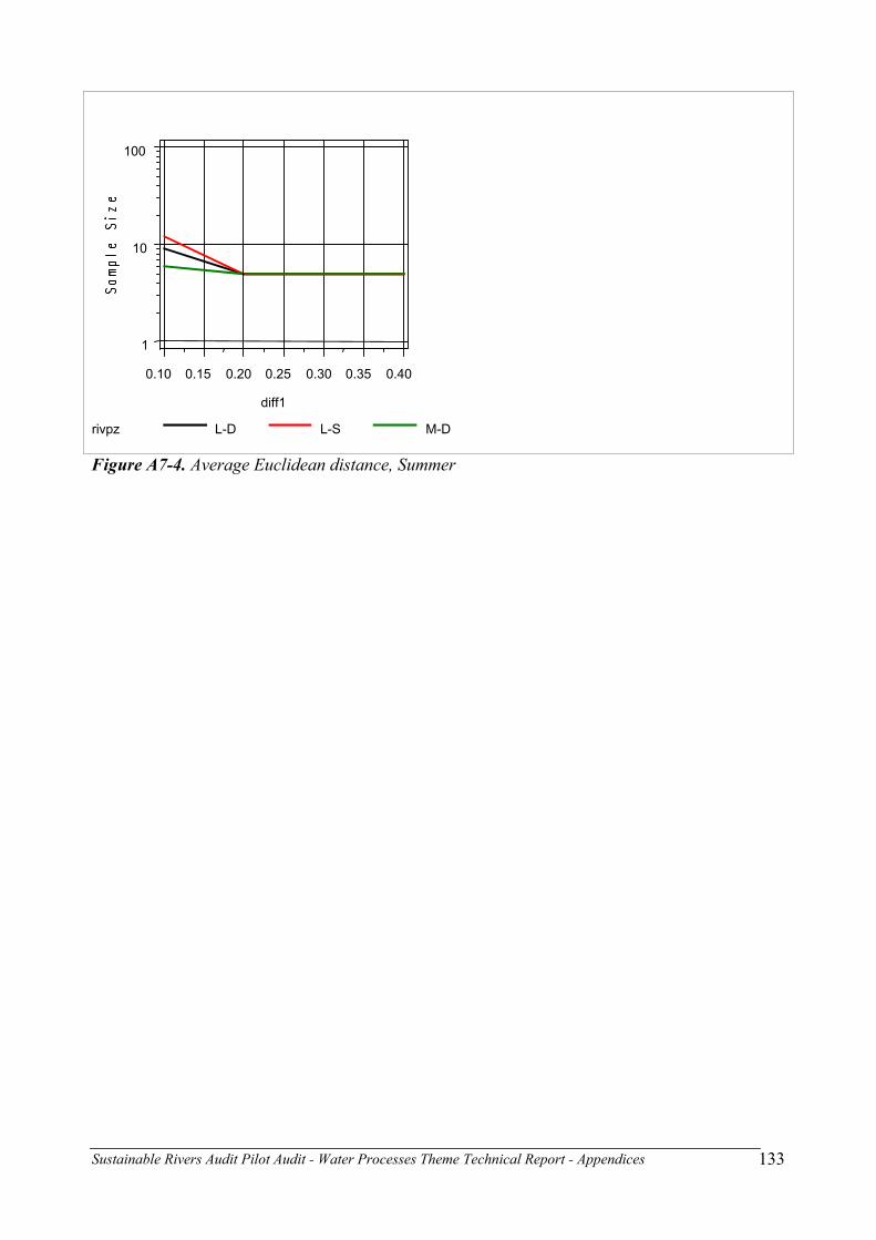
Sustainable Rivers Audit Pilot Audit - Water Processes Theme Technical Report - Appendices
133
Figure A7-4. Average Euclidean distance, Summer
rivpz L-D L-S M-D
1
10
100
diff1 0.10 0.15 0.20 0.25 0.30 0.35 0.40
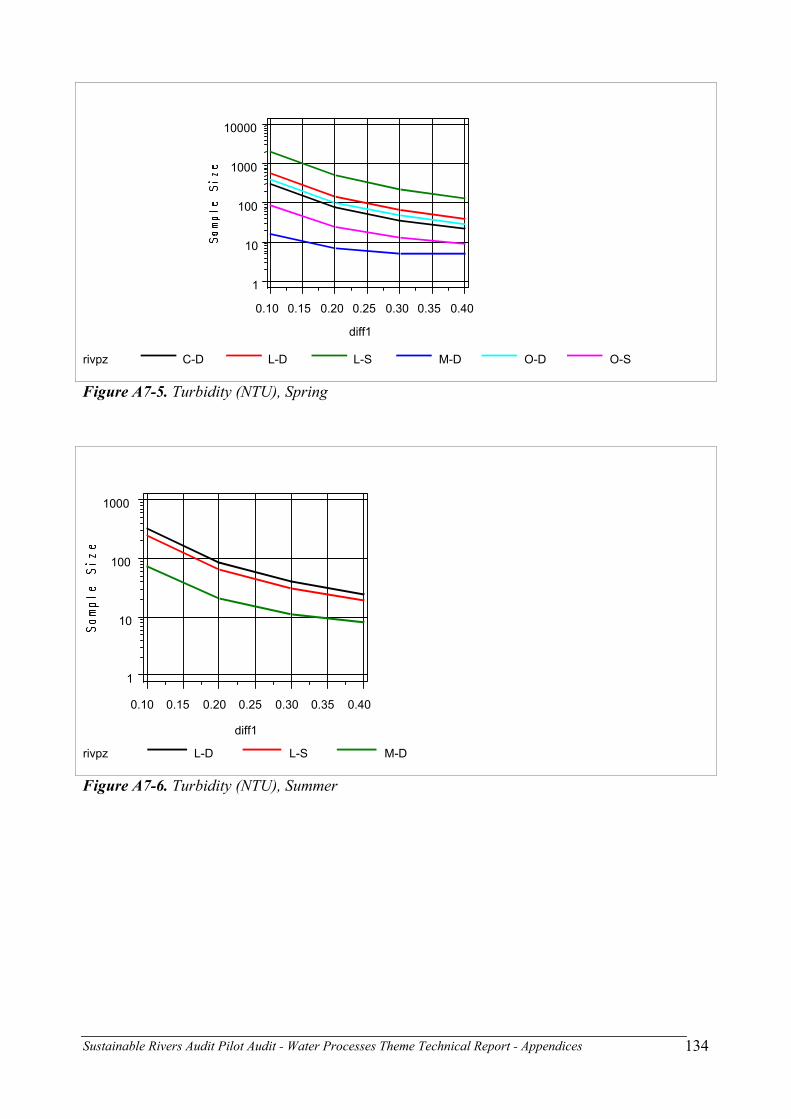
Sustainable Rivers Audit Pilot Audit - Water Processes Theme Technical Report - Appendices
134
Figure A7-5. Turbidity (NTU), Spring
Figure A7-6. Turbidity (NTU), Summer
rivpz C-D L-D L-S M-D O-D O-S
1
10
100
1000
10000
diff1
0.10 0.15 0.20 0.25 0.30 0.35 0.40
rivpz L-D L-S M-D
1
10
100
1000
diff1 0.10 0.15 0.20 0.25 0.30 0.35 0.40

Sustainable Rivers Audit Pilot Audit - Water Processes Theme Technical Report - Appendices
135
Figure A7-7. Temperature ( Cْ), Spring
Figure A7-8. Temperature( Cْ), Summer
rivpz C-D L-D L-S M-D O-D O-S
1
10
100
diff1
0.10 0.15 0.20 0.25 0.30 0.35 0.40
rivpz L-D L-S M-D
1
10
100
diff1 0.10 0.15 0.20 0.25 0.30 0.35 0.40

Sustainable Rivers Audit Pilot Audit - Water Processes Theme Technical Report - Appendices
136
Figure A7-9. pH, Spring
Figure A7-10. pH, Summer
rivpz C-D L-D L-S M-D O-D O-S
1
10
100
diff1
0.10 0.15 0.20 0.25 0.30 0.35 0.40
rivpz L-D L-S M-D
1
10
diff1 0.10 0.15 0.20 0.25 0.30 0.35 0.40

Sustainable Rivers Audit Pilot Audit - Water Processes Theme Technical Report - Appendices
137
Figure A7-11. Conductivity (µS/cm2), Spring
Figure A7-12. Conductivity (µS/cm2), Summer
rivpz C-D L-D L-S M-D O-D O-S
1
10
100
1000
10000
diff1
0.10 0.15 0.20 0.25 0.30 0.35 0.40
rivpz L-D L-S M-D
1
10
100
1000
diff1 0.10 0.15 0.20 0.25 0.30 0.35 0.40

Sustainable Rivers Audit Pilot Audit - Water Processes Theme Technical Report - Appendices
138
Figure A7-13. TN (mg/L), Spring
Figure A7-14. TN (mg/L), Summer
rivpz C-D L-D L-S M-D O-D O-S
1
10
100
1000
diff1
0.10 0.15 0.20 0.25 0.30 0.35 0.40
rivpz L-D L-S M-D
1
10
100
1000
diff1 0.10 0.15 0.20 0.25 0.30 0.35 0.40

Sustainable Rivers Audit Pilot Audit - Water Processes Theme Technical Report - Appendices
139
Figure A7-15. TP (mg/L), Spring
Figure A7-16. TP (mg/L), Summer
rivpz C-D L-D L-S M-D O-D O-S
1
10
100
1000
10000
diff1
0.10 0.15 0.20 0.25 0.30 0.35 0.40
rivpz L-D L-S M-D
1
10
100
1000
diff1 0.10 0.15 0.20 0.25 0.30 0.35 0.40

Sustainable Rivers Audit Pilot Audit - Water Processes Theme Technical Report - Appendices
140
Figure A7-17. DO (% saturation), Spring
Figure A7-18. DO (% saturation), Summer
rivpz C-D L-D L-S M-D O-D O-S
1
10
100
1000
diff1
0.10 0.15 0.20 0.25 0.30 0.35 0.40
rivpz L-D L-S M-D
1
10
100
diff1 0.10 0.15 0.20 0.25 0.30 0.35 0.40

Sustainable Rivers Audit Pilot Audit - Water Processes Theme Technical Report - Appendices
141
Figure A7-19. NOx (mg/L), Spring
Figure A7-20. NOx (mg/L), Summer
rivpz C-D L-D L-S M-D O-D O-S
10
100
1000
10000
diff1
0.10 0.15 0.20 0.25 0.30 0.35 0.40
rivpz L-D L-S M-D
10
100
1000
10000
diff1 0.10 0.15 0.20 0.25 0.30 0.35 0.40

Sustainable Rivers Audit Pilot Audit - Water Processes Theme Technical Report - Appendices
142
Figure A7-21. Chlorophyll-a (µg/L), Spring
Figure A7-22. Chlorophyll-a (µg/L), Summer
rivpz C-D L-D L-S M-D O-D O-S
1
10
100
1000
10000
diff1
0.10 0.15 0.20 0.25 0.30 0.35 0.40
rivpz L-D L-S M-D
1
10
100
1000
diff1 0.10 0.15 0.20 0.25 0.30 0.35 0.40

Sustainable Rivers Audit Pilot Audit - Water Processes Theme Technical Report - Appendices
143