i

António Augusto Mousinho Almadanim Santa

Marta

Degree in Environmental Engineering Sciences

Sustainable Aquaculture in Saldanha Bay,

South Africa

Dissertation submitted to obtain the degree of Master in

Environmental Management Systems

Thesis advisor: João Gomes Ferreira FCT-UNL

Jury:

President: João Gomes Ferreira

External examiner: João Lencart e Silva

Internal examiner: António Carmona Rodrigues

September 2015

ii

iii

António Augusto Mousinho Almadanim Santa

Marta

Degree in Environmental Engineering Sciences

Sustainable Aquaculture in Saldanha Bay,

South Africa

Dissertation submitted to obtain the degree of Master in

Environmental Management Systems

Thesis advisor: João Gomes Ferreira FCT-UNL

Jury:

President: João Gomes Ferreira

External examiner: João Lencart e Silva

Internal Examiner: António Carmona Rodrigues

September 2015

iv

Copyright © António Augusto Mousinho Almadanim Santa Marta, Faculdade de Ciências e

Tecnologia, Universidade Nova de Lisboa

A Faculdade de Ciências e Tecnologia e a Universidade Nova de Lisboa têm o direito, perpétuo

e sem limites geográficos, de arquivar e publicar esta dissertação através de exemplares impressos

reproduzidos em papel ou em forma digital, ou por qualquer outro meio conhecido ou que venha

a ser inventado, e de a divulgar através de repositórios científicos e de admitir a sua cópia e

distribuição com objetivos educacionais ou de investigação, não comerciais, desde que seja dado

crédito ao autor e editor.

v

AKNOWLOGMENTS

First of all, I want to thank my professor and thesis advisor Prof. João Gomes Ferreira for the

opportunity, the guidance, motivation, time spent, and availability. I have learned a lot with him.

I would like to express my very great appreciation to Dr. Grant Pitcher for the crucial data, the

kind help in reading and constructively criticizing my draft thesis, the precious support, and time

spent.

I would like to thank Dr. Sue Jackson for the kind availability, crucial help with data and contacts.

I also want to thank Mr. Schalk Visser, Mr. Vos Pinaar, and Mr. Kevin Ruck for the availability

and kind help with important data.

Thank you to my family for the patience, love, and comprehension.

I would like to offer my special thanks to my mother for the friendship, crucial support, and kind

help.

Thank you to my thesis companions Rita Pinto, João Mello, and José Pedro Vieira, for all

company and support.

Manny thanks to my very good friend André Pataco for the companionship, important help, and

support along this period.

I would like to offer my special thanks to Maria Apolónia for all the company, help, availability,

friendship, and support. Without her would not have been so fun to write a thesis.

vi

vii

ABSTRACT

Saldanha Bay, located near the coastal town of Saldanha, in Western Cape Province of South

Africa, possesses excellent conditions for mussel and oyster aquaculture. Its linkage with the

adjacent upwelling current system provides a very productive environment for phytoplankton

growth, and this has led to the development of a vibrant shellfish aquaculture industry. The main

objectives of this work are to develop a model which simulates the main ecological processes

within the Bay, to determine the Bay’s carrying capacity for mussel and oyster production, and

to produce a management tool for decision making.

Bivalve aquaculture has great growth potential and may be important for human food security as

mankind faces a projected need of an additional 30 X 106 tonnes per year of aquatic products by

2050. Bivalve aquaculture is organically extractive, and can additionally provide significant

ecosystem services in top-down control of eutrophication, and creation of structure for stimulating

biodiversity. When managed properly, this form of aquaculture has a very low environmental

footprint, mainly associated with organic enrichment of the sediment. This impact is even less

relevant in upwelling systems such as Saldanha Bay where particles tend to be flushed out in the

surface layer, and in all cases it must be borne in mind that by definition shellfish aquaculture

results in a net removal of seston from the water column.

This model was developed using EcoWin an object oriented approach to ecological modelling.

The model for Saldanha Bay was set up using oceanographic and water quality data collected

from Saldanha Bay, and culture practice information provided by local shellfish farmers. The first

step was the construction and calibration of the ecological model, in order to provide a general

description of the biogeochemical behaviour of the Bay, followed by the addition of the shellfish

aquaculture component.

EcoWin successfully reproduced the key ecological processes, correctly simulating a mean

phytoplankton biomass of 7.5 chl a L-1. The aquaculture module simulated an annual harvested

biomass of about 3000 t y-1, in good agreement with reported yield.

Six production scenarios were explored, for illustrative purposes:

- Increase in stocking density of shellfish

- Two alternatives for aquaculture development in particular areas of Saldanha Bay

- Prediction of the maximum production capacity of the Bay.

These results were analysed in terms of their impacts and potential.

viii

This study demonstrates the relevance of aquaculture-oriented ecological models in evaluating

different stakeholder-defined development scenarios, and their utility in avoiding the social and

environmental impacts of testing different scenarios in situ. The present application of EcoWin

shows great potential for supporting both water managers and industry in Saldanha Bay.

ix

Table of contents

1 Introduction ..................................................................................................................1

1.1 Carrying capacity ..................................................................................................2

1.2 Aquaculture potential.............................................................................................3

1.3 Aquaculture ..........................................................................................................4

1.4 Aquaculture around the world.................................................................................5

1.5 Importance of site selection for Aquaculture in Africa..............................................6

1.6 Shellfish aquaculture..............................................................................................6

1.6.1 Impacts of Shellfish aquaculture ......................................................................7

1.7 Production methods ...............................................................................................9

1.8 Oyster and Mussel biology .....................................................................................9

1.8.1 Mussels ....................................................................................................... 10

1.8.2 Oyster.......................................................................................................... 11

1.9 Legal Framework ................................................................................................ 11

1.9.1 Health and safety regulation .......................................................................... 12

1.9.2 General policy.............................................................................................. 12

1.10 Physical description of Saldanha Bay .................................................................... 13

1.11 Use conflicts ....................................................................................................... 15

1.12 Carrying capacity studies ..................................................................................... 15

1.13 Bivalve studies in Saldanha Bay ........................................................................... 16

2 Methods ..................................................................................................................... 19

2.1 Tools used........................................................................................................... 21

2.2 Data.................................................................................................................... 22

2.3 The Hydrodynamic model .................................................................................... 23

2.4 Forcing Functions ................................................................................................ 24

2.5 Temperature ........................................................................................................ 25

2.6 Salinity ............................................................................................................... 26

2.7 State variables ..................................................................................................... 27

x

2.8 Nutrients ............................................................................................................. 28

2.9 Suspended Matter ................................................................................................ 29

2.10 Phytoplankton ..................................................................................................... 30

2.11 Parameters .......................................................................................................... 31

2.12 Shellfish.............................................................................................................. 33

3 Results and Discussion ................................................................................................ 37

3.1 Water temperature ............................................................................................... 37

3.2 Salinity ............................................................................................................... 38

3.3 Dissolved Inorganic Matter .................................................................................. 38

3.4 Phosphate............................................................................................................ 40

3.5 Suspended Particulate Matter ............................................................................... 41

3.6 Particulate Organic Matter.................................................................................... 42

3.7 Phytoplankton ..................................................................................................... 42

3.8 Ecological model discussion................................................................................. 44

3.9 Model validation – Standard Scenario ................................................................... 45

3.10 Carrying capacity ................................................................................................ 50

3.10.1 Production carrying capacity ......................................................................... 50

3.11 Production scenarios: ........................................................................................... 55

3.11.1 Scenario 1 .................................................................................................... 55

3.11.2 Scenario 2 .................................................................................................... 56

3.11.3 Ecological impacts – Scenario 1 and 2 ........................................................... 56

3.12 Scenario discussion.............................................................................................. 58

4 Conclusion ................................................................................................................. 61

5 Bibliography ............................................................................................................... 65

xi

xii

LIST OF FIGURES

Figure 1 – Location of Saldanha Bay: 1) Southern Africa; 2) South Africa; 3) North from Cape

town; 4) Satellite view of Saldanha Bay. ................................................................................1

Figure 2 – Production methods illustration (left side) a tray method (right side); source: A.

Figueras (2004). ...................................................................................................................9

Figure 3 –Mytilus Galloprovincialis, shell illustration (left side) and picture (right side). Source:

A. Figueras, (2004)............................................................................................................. 10

Figure 4 – Crassostrea gigas shell illustration (left side) and picture (right side). Source: (Helm,

2005) ................................................................................................................................. 11

Figure 5 – Saldanha Bay illustration before iron ore construction. Source: B. W. Flemming,

(1977)................................................................................................................................ 13

Figure 6 – Saldanha Bay actual satellite picture. Source: Google maps................................... 14

Figure 7 – Simplified modelling framework used.................................................................. 19

Figure 8 – Conceptual model schematization. ....................................................................... 20

Figure 9 – Models box scheme organization. ........................................................................ 21

Figure 10 – Sampling stations spatial distribution inside the Bay. Source: Smith and Pitcher,

(2015)................................................................................................................................ 22

Figure 11 – Sampling stations for particle matter spatial distribution. Source:Monteiro and

Largier, (1999) ................................................................................................................... 23

Figure 12 – Hydrodynamic model illustration. ...................................................................... 24

Figure 13 – Temperature forcing functions used for each box. ............................................... 26

Figure 14 – Ocean boundaries salinity curves. ...................................................................... 27

Figure 15 – Boundary conditions for silica, phosphate, nitrite, nitrate and ammonia. ............... 28

Figure 16 – SPM (left side) and POM (right side) boundary conditions. ................................. 30

Figure 17 – Boundary phytoplankton biomass. ..................................................................... 31

Figure 18 – Temperature results for each box and measured data. .......................................... 37

Figure 19 – Salinity results for each box. ............................................................................. 38

Figure 20 – DIN results for each box. .................................................................................. 39

Figure 21 – Phosphate annual results for each box. ............................................................... 40

xiii

Figure 22 – SPM results for each box................................................................................... 41

Figure 23 – POM results for each box. ................................................................................. 42

Figure 24 – Phytoplankton results for each box. ................................................................... 43

Figure 25 – Phytoplankton results for boxes 3 and 4. ............................................................ 43

Figure 26 – Standard scenario harvested weight for each species for each area ....................... 46

Figure 27 – Oyster individual weight evolution in box 3 (left side) box 4 (right side), mussel

individual weight evolution in box 4 (bottom) ...................................................................... 46

Figure 28 – Oyster individual weight for 3 different POM scenarios: standard model (mean 1.1

mg L-1 POM); case 1 (mean 1.3 mg L-1 POM); case 2 (mean 0.9 mg L-1)................................ 47

Figure 29 – Difference between phytoplankton biomass before and after adding shellfish farms

to the model. ...................................................................................................................... 48

Figure 30 – Harvest results for different seeding intensities of mussel (left) and oyster (right),

inside Small Bay ................................................................................................................ 51

Figure 31 – Number of seeds in Small Bay for the two maximum scenarios ........................... 51

Figure 32 – Harvested shellfish in live weight and wet meat in tonnes for the maximum production

scenarios in Small Bay........................................................................................................ 52

Figure 33 – Oyster harvested weight per seeded weight inside Big Bay .................................. 53

Figure 34 – Comparison of harvested live and wet meat weight of oyster in Small and in Big Bay.

......................................................................................................................................... 53

Figure 35 – Average phytoplankton biomass inside each box ................................................ 54

Figure 36 – Comparison of maximum production capacity in each box .................................. 55

Figure 37 – Scenario 2 annual shellfish harvest. ................................................................... 55

Figure 38 – Scenario 2 oyster annual harvest in box 4. .......................................................... 56

Figure 39 – Average phytoplankton biomass for each box and each scenario .......................... 57

xiv

LIST OF TABLES

Table 1- Nitrogen removal costs for different removal strategies, source: Ferreira and Bricker,

(2015)..................................................................................................................................7

Table 2 – Stations used for each box group. ......................................................................... 25

Table 3 – Initial salinity conditions for each box. .................................................................. 27

Table 4 – Initial conditions for each box .............................................................................. 29

Table 5 – Initial conditions for each box to POM and SPM ................................................... 30

Table 6 – Initial phytoplankton biomass for each box............................................................ 31

Table 7 – Phytoplankton parameters used............................................................................. 32

Table 8 – Suspended particle matter used parameters. ........................................................... 33

Table 9 – Companies working in Saldanha Bay, respective annual production and licensed area.

......................................................................................................................................... 34

Table 10 – Mussel and oyster production, number of seeds, farm area, seed and harvested shellfish

weight. .............................................................................................................................. 35

Table 11 – Comparison between measured average DIN and mean DIN results for each box. .. 39

Table 12 – Measured average phosphate comparison with mean results phosphate for each box.

......................................................................................................................................... 40

Table 13 – Modelled and estimated production for each box, organized in species. ................. 45

Table 14 – Bivalve ecosystem removals for each farmed box. ............................................... 48

Table 15 – Mean phytoplankton comparison, before and after adding the farms into the model, in

boxes 3, 4, 7, and 8. ............................................................................................................ 49

Table 16 – Total scenario removal for each species and total ................................................. 50

Table 17 – Scenario 4 ecological removals for each shellfish species. .................................... 57

xv

1

1 Introduction

The government of South Africa approved a National Development Plan, Vision 2030 that aims

to reduce poverty, unemployment and inequality by this date. For the present government,

“aquaculture’s role and contribution to food security is central to addressing poverty,

unemployment, and inequality” (National Aquaculture Policy Framework, 2013).

The coastal Town of Saldanha, in South Africa, is located near a Bay which has excellent

conditions for mussel and oyster culture. This Bay is home for farms of both species, with an

annual total production of about 2400 tonnes. Saldanha Bay is located in the southwest coast of

the country, forming part of the Benguela Current Large Marine Ecosystem. Due to the upwelling

in Benguela current system, this Bay has nutrient rich waters, providing a productive environment

for phytoplankton growth (Olivier et al., 2013).

Figure 1 – Location of Saldanha Bay: 1) Southern Africa; 2) South Africa; 3) North from Cape town; 4) Satellite

view of Saldanha Bay.

2

The central question addressed in this thesis is whether the current farming activities are working

at the Bay’s carrying capacity defined as the maximum production achievable without affecting

the ecosystem, including other such as fisheries to an unacceptable level. This question is

developed into four main objectives: (1) to analyse the carrying capacity of Saldanha Bay for

shellfish production at the scale of the Bay; (2) to describe the main environmental variables and

processes and their interactions with the aquaculture activities; (3) to develop different production

scenarios; (4) to illustrate how ecological models can support management decisions for Saldanha

Bay.

1.1 Carrying capacity

Carrying capacity has been interpreted in a range of different perspectives, such as, physical,

social, economic and environmental. Davies and McLeod (2003), for instance, considered bivalve

carrying capacity as “the potential maximum production a species or population can maintain in

relation to available food resources” (production perspective) as Lindsay G. Ross et al. (2013)

defined carrying capacity as “the level of resource use (…) that can be sustained over the long

term by the natural regenerative power of the environment” (an ecological perspective). Inglis,

G.J. et al. (2000) defined carrying capacity in the broader and more important perspective,

considering that carrying capacity can be interpreted in four categories: physical, production,

ecological and social carrying capacity;

With a similar perspective, FAO defined in 2013 an approach to aquaculture, which has three

principles: (1) aquaculture development without degradation of the ecosystem beyond its

resilience capacity; (2) improvement of human well-being and equity for all relevant stakeholders;

and (3) development in the context of other policies, sectors, and goals.

Physical carrying capacity concept defines an area, available and physically suitable for a certain

type of aquaculture. This concept depends on the match on needs of the target species and the

characteristic of the selected area, and uses characteristics such as depth, temperature, salinity,

and substrate type. Production carrying capacity is the optimization of the production level for

the target species (marketable cohort within a specific time-frame). This is mainly dependent on

natural processes, e.g. primary production and hydrodynamics. Ecological carrying capacity is

the maximum production that can be accomplished without having an unacceptable

environmental impact. Social carrying capacity is the level of production that causes unacceptable

social impacts. It comprises the trade-offs between stakeholders in order to meet the demands of

population and environment (McKindsey et al., 2006).

3

The individual use of either ecological or production carrying capacity criteria is not adequate for

shellfish farming management. The strict ecological perspective does not allow any change in the

receiving environment and the production capacity does not consider any environmental criterion

(Guyondet et al., 2010). A general carrying capacity should be a compromise between production

and ecological carrying capacity (Gibbs, 2007; McKindsey et al., 2006), the ultimate goal must

be the development of the most productive farm without compromising its long term viability nor

the ecosystem stability (Guyondet et al., 2010). McKindsey et al. (2006), uses the definition of

G.J. et al. (2000) to build a decision framework that integrates its four categories to determine the

overall capacity for bivalve aquaculture. This framework uses physical carrying capacity,

production carrying capacity, ecological carrying capacity and social carrying capacity, in this

order. In this way it is possible to calculate the general carrying capacity for a certain location.

This study intends to combine physical, production, and ecological carrying capacity concepts,

using these methods. The generic carrying capacity should also include both local and system

scale approaches (Smaal et al., 1997). The system scale is used to determine the propagation of

local effects (Guyondet et al., 2010) and the local scale is used for farm management

considerations (Ferreira et al., 2007; Strohmeier et al., 2008).

The importance given to sustainable development and consequently to ecological carrying

capacity varies around the globe, for instance, the developing and underdeveloped countries are

less committed to it (Aguilar-Manjarrez et al., 2010). Carrying capacity is a central concept in

ecosystem-based management, as it avoids “unacceptable changes” in the natural ecosystem and

social structures by setting upper limits to aquaculture considering environmental limits and social

acceptability for aquaculture. It is very important to evaluate the carrying capacity to an area

before establish large-scale shellfish farms, to ensure a suitable food supply for the expected

production and to avoid and minimize ecological impacts (Ferreira et al., 2008).

1.2 Aquaculture potential

In 2050 the Human population should reach 9700 million people (United Nations, 2015), which

is above the earth’s estimated maximum carrying capacity (Cohen, 1995). A very important

question to science is whether it is possible to increase food production to fulfil the human needs

for such a large number of people. The present population is already under water stress and global

warming worsens this situation. Agriculture production to 9700 million people demands bigger

water resources and the rise of agricultural production for non-food supplies augments the

problem. On the top of this, global fisheries landings have been declining. Under these

circumstances mariculture, the least fresh water dependent food producer, might have an

important role feeding mankind in the future. (Duarte et al., 2009).

4

Fish have the highest protein content in their flesh of all food animals. They are more efficient

than any terrestrial farmed animals, converting feed to body tissue. Besides all this, aquatic

animals discharge two to three times less nitrogen to the environment when compared to terrestrial

food production systems (Costa-Pierce, 2010).

1.3 Aquaculture

Aquaculture is the cultivation of aquatic organisms including finfish, shellfish, and plants.

Cultivation involves the enhancement of natural production processes such as feeding, stocking,

and protection from predators. The act of farming means that there is some kind of ownership,

individual or corporate, over the stock (Handbook of Fishery Statistical Standards.).

Aquaculture can take place on land or in waterbodies; the latter include freshwater such as rivers

or lakes, brackish water such as estuaries, and fully saline water such as Bays and open coastal

water. In onshore aquaculture, ponds are most widely used for production. Cage based

aquaculture for freshwater has bigger impacts. Although the use of ponds in brackish water faces

substantial competition for space and environmental problems, ocean onshore production has

developed in some areas where it wouldn’t be possible otherwise. The coastal floating cage farms

have proved to be the most effective production system. The production of seaweed and marine

molluscs has been developing since the 1990s to specialized techniques allowing it to grow

significantly. (Bostock et al., 2010)

Growth of freshwater aquaculture is increasing pressures on natural resources, mainly water,

feeds, and energy. Most freshwater aquaculture involves water intake from the environment and

post-production effluent stream. Given the increasing pressures on fresh water supplies greater

use of brackish and marine water is expected in the future (Bostock et al., 2010).

Aquaculture in coastal waters can have serious environmental problems as well. Shrimp farming,

for instance, may cause serious environmental impacts. Marine cage finfish aquaculture can have

impacts on biodiversity and the ecosystem, in bigger scales it can have impacts in the sediments

beneath the cages, release of nutrient, or chemical wastes, or the escape or release of fish with

diseases. The most immediate problem, however, is with competition for uses, such as boating

and navigation, recreation, preservation of seascape and tourism. (Bostock et al., 2010)

5

Most mollusc farming needs no feed inputs and the majority of freshwater fish production uses a

low-protein, grain-based diets, and organic fertilizers. Much of the marine species crustaceans

and other fish aquaculture use a higher quality diet usually containing fish meal and fish oil. Some

aquaculture, such as tuna fattening needs small pelagic fishes. Although not essential, feeds for

herbivorous and omnivorous species frequently contains fish meal and oil. The rapid expansion

of carnivorous species could also increase pressure on fish meal and oil supplies. Overall the

supplies of fish meal and oil won’t be sufficient to meet the increasing demands for aquafeed

ingredients. Nevertheless this isn’t expected to be a great constraint, but the demand for

alternative feed materials will increase. (Bostock et al., 2010)

There are several approaches to integrate aquaculture with other activities, such as, fisheries,

agriculture, and Integrated Multi-Trophic Aquaculture (IMTA). Many aquaculture systems need

captured fish for its feeds and aquaculture has an important role in fisheries capture enhancements,

releasing farmed fish. Their release can however represent significant ecological and genetic risk

to wild fish stocks.

The integration of fish species from different trophic levels can be made in the same water body

or with some other water based linkage. This combination generates a synergetic relationship that

acts as a bioremediation measure. A perfect system of this nature would be environmentally

neutral. Such methods face a number of challenges, such as species selection, economic value,

and existing regulations for aquaculture.

The integration of aquaculture and agriculture is most common in developing countries, as it

diminishes the risks of mono culture. These systems use the synergy between systems to diversify

production and to enhance productivity.

1.4 Aquaculture around the world

The aquaculture sector has expanded strongly over the past 6 years, from 47 million tonnes in

2000, to around 64 million tonnes in 2011 in 2008 aquaculture was responsible for about 37% of

the world’s fish food supply. However, Asia accounts from 89% of the world production .

Therefore the world does not have a massive development of aquaculture outside China. Outside

China aquaculture contributes only for 23% of world fish products. It is also important to mention,

that in 2008 freshwater fish represented about 60% the aquaculture production.

6

With few exceptions such as Norway, aquaculture development in developed countries is very

limited. In these countries aquaculture growth has been limited by user conflicts, access to sites,

complicated regulatory regimes, lack of government investment, consumer disinterest, and lack

of aquaculture education. In the poorest nations, aquaculture development has not occurred

significantly, except for, Bangladesh, India, Vietnam, and Egypt (Costa-Pierce, 2010).

1.5 Importance of site selection for Aquaculture in Africa

With the decline of fish stocks worldwide, aquaculture is looked at as an important solution,

especially for Africa, in which many areas contain an undernourished population dependent on

marine and freshwater fishing for incomes (Wit, 2013). The development of aquaculture needs to

be planned in order to diminish environmental and social impacts, and to predict optimum

production scenarios (Byron and Costa-Pierce, 2013). The use of GIS is the most efficient, cheap,

and fast way to select sites for aquaculture. It involves the identification of economically, socially,

and environmentally available areas (McLeod et al., 2002). The use of these models requires

regional data and the costs of data collecting in the sea are often high. Given the economic

panorama in most of the African countries, this kind of expenses can be a limiting factor.

Therefore, use of remote sensing has great potential and importance to the use of GIS and in this

region, to determine the viability of some projects and decision making (Wit, 2013).

1.6 Shellfish aquaculture

Non fed aquaculture such as the production of shellfish has different concerns than fed

aquaculture. Filter feeding shellfish do not need artificial food, consuming mostly microalgae and

other suspended organic materials, making them an especially attractive form of aquaculture. This

type of aquaculture provides vital social and ecological services, such as nutrient removal and

habitat enhancement (Costa-Pierce, 2010; Brigolin et al., 2009). They reduce water turbidity

which may improve the condition of submerged aquatic vegetation (SAV), remove N from

eutrophied systems by incorporating a proportion of it in tissues, and help to control or prevent

harmful algal blooms. Public health standards for aquaculture demand clean waters, requiring

increased water quality monitoring at farm sites. Shellfish are farmed in well-defined areas, in

structures that may provide a protection or habitat for other species.

7

Bivalves may have an important role in the nutrient credit programs. There is an excess of nutrient

inputs to the water in numerous areas of the European Union (EU) and North America, mostly

from non-point sources. The concept of a nutrient credit program is to reduce the nutrient loads

by using a market based approach. This approach uses economic incentives to reduce nutrient

discharges, by attributing credits to the involved polluters, which they can sell if come to reduce

their emissions. In this way, the ones who can reduce their emissions by a lower price can sell

their remaining credits. This could create new monetary income opportunities for farmers, who

can remove nutrients from the water at a low price, as table 1 shows. The shellfish nutrient

removal is one of the cheapest methods of doing it as it has great potential. These programs are

already in use in some parts of the US, although not in the EU nor African countries, such as

South Africa.

Table 1- Nitrogen removal costs for different removal strategies, source:(Ferreira and Bricker, 2015)

Non-point-source nutrient management strategy Cost (euro kg-1 N)

Shellfish 11 – 278

Agricultural 0.2 – 870

Urban stormwater 56 – 6720

Wastewater treatment upgrades 0.9 – 14 093

Wetlands 1.1 – 396

Other 5.2 – 404

1.6.1 Impacts of Shellfish aquaculture

Despite the benefits of shellfish aquaculture, it may accelerate the deposition of suspended

materials through the production of faeces and pseudofaeces (Chamberlain et al., 2001). These

animals filter suspended material from the water, digest it, and reject a portion of it as compact

faeces. It is also common that bivalves reject a part of the filtered material before its ingestion, in

a less compact mass called pseudofaeces (Haven and Morales-Alamo, 1972). Both these particles,

settle much faster than particles of smaller grain size. Such consolidated particles are termed

biodeposits. (Haven and Morales-Alamo, 1966).

8

Many studies have been made to determine the impacts of bivalve farming. The biodepositon

process results in the enrichment of organic materials in sediment and this may cause the reduction

of the level of dissolved oxygen in the lowest layer, increase levels of sulphides, changes of

benthic assemblages and azoic conditions (Zhang et al., 2009), resulting in the appearance of

opportunistic species and biodiversity decrease in the substrate (Stenton-dozey et al., 1999).

When close to the production carrying capacity, shellfish aquaculture may reduce the zooplankton

availability, by over-compete it in phytoplankton consumption. This might reduce some higher

trophic level fish, which would depend on zooplankton (Jiang and Gibbs, 2005), the introduction

of exotic species and proliferation of certain species such as starfish and jellyfish are possible

impacts as well (McKindsey et al., 2011).

Souchu et al. (2001) tested the effects of shellfish farming in the water column in Thau Lagoon

in Mediterranean France. A nutrient surplus was observed in the water column near the farms, as

a cause of plankton removal by shellfish. Thau Lagoon however, has very different physical

conditions than Saldanha Bay, as a Mediterranean lagoon with low tides, wind, and wave events.

Chamberlain et al. (2001), studied the effects of mussel farming on the surrounding sediments in

Southwest Ireland in two different farms, and obtained different results for each. One (lower

current speed) showed organic material enrichment and an impoverished benthic community as

the other showed no significant impacts. Studies on suspended shellfish (mussels and oysters)

culture in Tasmania (Crawford et al., 2003), and Nova Scotia (Grant et al., 1995) found little

impact on the benthic community. Stenton-Dozey et al. (2001) studied the impacts of mussel

farms in Saldanha Bay and found significant impacts on the substrate, such as anoxic conditions,

presence of opportunistic polychaetes and a significant reduction in macrofaunal biomass. Zhang

et al. (2009) studied the impacts of intensive shellfish and seaweed farming in Sanggou Bay,

China and found some biochemical and biological changes, but these were considered low impact

over a longer term. Kaspar et al. (1985) studied the impacts of mussel production in Kenepuru

Sound, New Zealand and it found a strongly affected benthic community, with biodiversity

reduction and a surplus of nitrogen in the water column.

The effects of shellfish biodeposition may or may not be significant, as the examples show. This

depends greatly on the dispersion of biodeposits, which is dependent on water depth, current

velocity and on settling speed. The farm’s production intensity, scale, and methods are also very

important as it will affect the biodeposit input (Chamberlain et al., 2001; Zhang et al., 2009). The

use of methods such IMTA may help reduce the impacts and make the production more

sustainable. Zhang et al. (2009) showed how shellfish and seaweed IMTA could be more

sustainable, as the seaweed produced oxygen that helped to meet benthic demand and avoid

anoxic conditions.

9

1.7 Production methods

The main cultivated species in Saldanha Bay are the oyster Crassostrea gigas and the mussel

Mytilus galloprovincialis, and constitute the focus of this study the two species are cultivated

using similar techniques: raft culture; long-line culture; rack culture; on-bottom culture; and

perforated plastic trays/mash bags. There are several variations of the same methods with different

materials. Figure 2 illustrates some of these methods.

Figure 2 – Production methods illustration (left side) a tray method (right side); source: A. Figueras (2004).

Mussel seed can be collected manually or using collecting ropes where it attaches naturally,

hatchery is not common for mussels. The mussels are afterwards grown on ropes, which can be

suspended from rafts, wooden frames, or longlines of floating plastic buoys. Mussel can be

harvested around the year, but this should be avoided during spawning periods.

Oyster seeds can be obtained through artificial collectors too or in hatcheries, which can force the

animal spawning, having seeds available all year round. The oysters can be set in mesh bags or

perforated plastic trays in the low intertidal zone, or in suspension ropes as with Mytilus

galloprovincialis. They are also not harvested during the spawning period, for lower quality meat.

(Aypa, n.d.; Garrido-Handog, n.d.)

1.8 Oyster and Mussel biology

The phylum Mollusca is of great importance in the animal kingdom as it is one of the largest and

most diverse groups. Molluscs are soft-bodied animals, but most include a hard protective shell.

Most molluscs have a basic body plan inside the shell, which includes a heavy fold tissue named

the mantle and a large muscular foot. The mantle encloses all the interior organs and the foot is

generally used for locomotion.

10

The class Bivalvia is one of six Mollusc classes and includes all the animals enclosed in two shell

valves, such as, the mussel, oyster, clam, and scallops. The shell serves as protection for predators,

a skeleton for the attachment of muscles, and it helps to avoid mud and sand into the mantle cavity

in burrowing species. Between bivalve species the shell’s form, colour, and markings diverge

significantly.

Bivalves are filer feeders and feed mainly on phytoplankton, they have the ability to select the

food filtered from the water. The food is bounded with mucous, passed to the mouth, and

sometimes rejected and discarded out of the animal, when is named “pseudofaeces” (Helm et al.,

2004).

1.8.1 Mussels

Mussels have two shells, similar in size and approximately triangular. Shell colour varies with

age and location of the animal. The two shells are held and articulated together at the anterior

through a ligament. The foot serves to attach the mussel to the substrate or other mussels, by the

secretion of tough filaments in the ventral part of the mussel (Gosling, 2008).

Mussel length varies under the environmental conditions over which it lives. Under optimal

conditions a mussel can reach a much bigger length than when exposed to marginal conditions.

The shells of closely packed mussels have higher length to height ratios, from those in less

crowded sites (Gosling, 2008).

The mussel species used for this study is Mytilus galloprovincialis, or Mediterranean mussel.

These species live in waters with temperature ranging from 10 to 20°C, salinity around 34‰ psu.

This species can reach up to 15cm but the normal length is 5-8cm. (Figueras, 2004). Figure 3

illustrates this species shell.

Figure 3 –Mytilus Galloprovincialis, shell illustration (left side) and picture (right side). Source: A. Figueras,

(2004)

11

1.8.2 Oyster

The European flat oyster, Ostrea edulis, valves are roughly circular, one valve is flat and the

other cupped, and they are hinged together by a tense ligament on the dorsal side. The flat side of

the shell is attached to the substrate. The American Eastern oyster, Crassostrea virginica, has a

more lengthened shape than the European one, and the upper shell more profoundly cupped. The

shell is for both species thick and solid. In general the Ostrea edulis has a maximum shell height

of 100mm as Crassostrea virginica ca reach 350mm length (Gosling, 2008).

The species studied in this work is Crassostrea gigas, also known as the Pacific oyster, originally

from Japan. This bivalve is an estuarine species that prefers hard bottom substrate, from the lower

intertidal area to depths of 40m. The optimal salinity range is 20 – 25 ‰, but it can live in salinities

between 10‰ psu and 35‰ psu. It tolerates temperatures from -1.8 to 35°C and it can achieve

commercial size in 18-30 months when in good conditions. Its rapid growth and wide range of

tolerance to environmental conditions, made this oyster the preferred choice for many farmers

worldwide. This oyster has an elongated, cupped, and extremely rough shell, as Figure 4

illustrates. The maximum length is 30 cm, but the normal length ranges between 8 to 15 cm (Helm,

2005; Pauley et al., 1988).

Figure 4 – Crassostrea gigas shell illustration (left side) and picture (right side). Source: (Helm, 2005)

1.9 Legal Framework

In an ideal scenario, governments regulate processes and the import export linked to mariculture,

in order to protect the sector from user conflicts, overexpansion, and biosecurity risks. The state

should also make policies to promote sustainable development and local participation. It may also

supply investigation funding, sponsor the industry development, or provide operational loans

(Britz et al., 2009).

12

The most relevant legislation in South Africa consists of three acts: (i) the Marine Living

Resources Act of 1998, was written for fisheries and is under revision to improve its applicability

for aquaculture; (ii) the National Environmental Management: Biodiversity Act of 2004, regulates

farming of non -native species; (iii) the National Environmental Management: Integrated Coastal

Management Act of 2008, with focuses on a sustainable management of coastal waters; (Olivier

et al., 2013)

1.9.1 Health and safety regulation

Oyster are often consumed live and raw, and mussels easily accumulate algal biotoxins (Pitcher

et al., 2011). Therefore, health and hygiene standards for culture, packaging, and sale are very

important for consumer safety. The South African Live Molluscan Shellfish Monitoring and

Control Program carries out regular and compulsory monitoring for heavy metals, biotoxins, and

human microbial pathogens.

1.9.2 General policy

The most pertinent national policies to aquaculture are: the Policy for the Development of a

Sustainable Marine Aquaculture Sector in South Africa (PDSMAS), from the Department of

Environmental Affairs and Tourism in 2007; the National Industrial Policy Framework (NIPF);

the Western Cape Aquaculture Development Initiative; and Generic Environmental Best Practice

Guideline for Aquaculture Development and Operation in the Western Cape; South Africa has

policies towards the development of sustainable and competitive aquaculture, the co-ordination

between the different state Departments involved (PDSMAS) and towards financial and technical

support to small, medium, and micro enterprises (NIPF). (Olivier et al., 2013)

Olivier et al., (2013) carried out a series of interviews with directors of all bivalve marine farms

in Saldanha Bay who stated that the aquaculture sector is over-regulated. The producers in South

Africa are required to obtain five permits: Mariculture permit; Fishing vessel permit (for each

vessel used); Fish Processing Establishment Permit; Spat and seed importation permit; and export

permits for those who wish to export. In Saldanha Bay farmers lease water space from the

National Ports Authority (Portnet), the directors and state representatives interviewed described

the fees from Portnet excessive, the most expensive in the world. The National Aquaculture Policy

Framework for South Africa 2013, intends to correct several problems inside the country’s

aquaculture sector, namely to simplify the permitting process, and to pass food quality and safety

legislation for compliance with international standards.

13

1.10 Physical description of Saldanha Bay

Saldanha Bay is located on the South African west coast, about 100km north of Cape Town, and

is directly connected to the shallow tidal Langebaan Lagoon. The Bay and the lagoon are

considered areas of great biodiversity in the country. A number of marine areas around the Bay

have been declared protected, and Langebaan Lagoon and much of the surrounding land are part

of the West Coast National Park (Clark et al., 2012).

Saldanha Bay consists of an outer Bay and an inner, shallower Bay (Figure 5). This was

considerably altered in in the 1970’s with the construction of a causeway for iron ore and oil

terminals (Figure 6). This created two sectors: the Big and Small Bay (Pitcher et al., 2015; Clark

et al., 2012)). The area of the lagoon is about 40 km2 (Flemming, 1977) the Bay’s area is about

45 km2 (Grant et al., 1998).

Figure 5 – Saldanha Bay illustration before iron ore construction. Source: B. W. Flemming, (1977)

14

Figure 6 – Saldanha Bay actual satellite picture. Source: Google maps.

South Africa is exposed to strong climatic influences: The South Atlantic Ocean high pressure

system that lies to southwest; The Indian Ocean high pressure system in the east; and the

westerlies wind system to south where low pressure systems develop; This results in strong wind

systems along the country (Kruger et al., 2010). The prevailing winds tend to be equatorward,

parallel to the coast, inducing upwelling (Harris, 1978). During the winter the northwesterly winds

dominate.

Upwelling is a phenomenon that occurs when a surficial water layer drives away from the coast,

and the bottom cold and nutrient rich water comes to the surface, replacing the upper layer near

the coast. The cause of upwelling can be wind stress, parallel to coast that results in a current

opposite to the coast (Coriolis Effect), or when the water near the coast is warmer than the ocean

water resulting in a similar current effect (Monteiro and Largier, 1999).

The upwelling season in Benguela lasts around 10 months, from August to May at which time the

Bay is typically stratified. The local winds can affect the Bay waters in two ways. It drives

upwelled bottom water into the Bay, enhancing thermal stratification. On the other hand, these

winds can drive the vertical mixing and entrainment of intruded upwelled waters. Typically

coastal winds drive upwelling and local winds mixing. In Saldanha Bay, upwelling process is

very important for water renewal, and during such events the residence time is half the normal

time (Monteiro and Largier, 1999). Nutrient input into the Bay is largely dependent on the

advection of cold NO3- rich bottom water into the Bay and the vertical turbulent flux across the

thermocline.

Monteiro and Largier, (1999) propose a 4 phase explanation of the upwelling process in the short

term. First the equatorward wind drives vertical mix and upwelling, there is an intrusion of the

Small Bay

Big Bay

15

cold bottom water, in phase three there is formation of a thermocline, and in the last phase the

bottom cold water drains away. During phase 2 there is nutrient availability and the only limitation

for phytoplankton production is light. During phase 3, thermocline formation limits NO3- supply

to the surface layer and nutrient availability becomes the main limitation to production.

1.11 Use conflicts

Water quality is very important in aquaculture, as it influences the farmed species health. Good

water quality results in an increased production efficiency and product quality (Boyd and Tucker,

2012) beyond that shellfish producers must meet public quality standards for water quality and

are subject to quality control in several countries including South Africa. Therefore farmers

cannot tolerate any activity that changes their farms’ water quality (Shumway et al., n.d.). Filter-

feeding aquaculture uses an important resource, space, by which it can conflict with other

activities, such as, wild stock fisheries, mineral extraction, and tourism, as it may occupy areas

where these activities will not be allowed to occur (Gibbs, 2004). Therefore shellfish aquaculture

can conflict with all activities that may compete for space use or affect water quality.

There are a number of activities in Saldanha Bay that can affect water quality, such as:

- Port

- Liquid petroleum facility

- Shipyard

- Reverse osmosis desalinization plants

- Sewage discharges

- Fish processing plant

- Urban development

- Tourism

The port expansion, requires extensive dredging and marine blasting, and the fish processing

factories discharge effluents with significant quantities of organic material, which can lead to

deterioration in water quality in the Bay. Ships using the Port of Saldanha discharge large volumes

of ballast water, which represents a great risk, of introducing alien species and contaminants into

the Bays water. Urban development increases the volume of storm water entering the Bay, which

is a major source of non-point pollution and typically contains contaminants such as, bacteria,

nutrients, hydrocarbons, pesticides, solvents, metals, and plastics. The population growth results

in increased pressure through increased waste waters (Clark et al., 2012).

1.12 Carrying capacity studies

Many studies calculate carrying capacity for finfish and shellfish production using different

scales, sites, and methods. Most of these are studies that use spatially resolved ecological models,

16

which divide the ecosystem in boxes and simulate hydrodynamic transport (Duarte et al., 2003).

Bivalves are dependent on the ecosystem’s primary production, and therefore, mathematical

models can be very useful in understanding and simulate the interactions in such ecosystems. The

most commonly used models are the bio-physical ones that consider the influence of

hydrodynamics on transport and mixing, biochemistry, and population dynamics (Dowd, 2005;

Franco et al., 2006). These models offer considerable potential for simulating the growth of

species, and determining of the conditions providing best growth potential, both very useful to

aquaculture management.

Several studies built ecological models, trying to determine the carrying capacity for a certain

species production in different study sites all around the world: Ferreira et al., (2008) for mussel

and oyster production in four loughs in Northern Ireland; Filgueira et al., (2014) for oyster

production in the Richibucto Estuary, eastern Canada; Brigolin et al., (2009) mussel farming in

northern Adriatic Sea in Italy; Luo et al., (2001) for menhaden production in Chesapeake Bay;

Duarte et al., (2003) Sungo Bay, Shandong Province, People’s Republic of China for IMTA of

bivalve shellfish and kelp; Bacher et al., (1997) for mussel in Marennes-Oléron Bay, France;

Guyondet et al., (2010) mussel production in Grande-Entrée Lagoon (GEL) ecosystem, Canada.

1.13 Bivalve studies in Saldanha Bay

There are a number of studies relevant for shellfish production carrying capacity in Saldanha Bay.

Pitcher et al., (2015) investigated the Bay’s productivity using the light-and-dark bottle oxygen

method, and compared methods on primary production determination. Henry et al., (1977) studied

the seasonal variability of primary production in Saldanha Bay and Langebaan Lagoon Monteiro

and Brundrit, (1990) analysed the effects of the variable characteristics of coastal waters on

chlorophyll annual and monthly variance. Pitcher and Calder, (1998) estimated phytoplankton

biomass in the Bay, analysing the physical and chemical environment that conditions it. These

studies focus mainly on phytoplankton production, which is important because phytoplankton

stands as the available food for shellfish production. Grant et al. (1998) studied Saldanha’s Bay

carrying capacity, using the Bay’s carbon budget. It compared an estimate of phytoplankton

carbon production in the Bay with an estimate of the phytoplankton carbon consumption by the

existing mussel production.

17

Other studies regarding shellfish production were made for Saldanha Bay impact of mussel

culture on the substrate by Stenton-Dozey et al., (2001); Stenton-dozey et al., (1999), (see above).

Probyn et al. (2000) studied the physical factors causing the seasonal appearance of toxic algal

blooms in the Bay. Probyn et al., (2001) summarize the effects of these algal blooms on shellfish

production. Anderson et al., (1999) studied the potential of fish effluents for the production of

Gracilaria gracilis, for increasing both production efficiency and nutrient removal from the

water.

Olivier et al., (2013) investigated the possible social benefits of cultivating oysters and mussels

in Saldanha Bay at carrying capacity. Mussel production totals of one project are combined with

projected potential estimates determined in other studies to determine carrying capacity.

18

19

2 Methods

This work focused on the construction of an ecological model. This model aims to simulate the

ecological dynamics of Saldanha Bay, creating a powerful management tool for system analysis.

The model may be used to predict how the different ecological variables would respond or change

to the introduction of new inputs, and to simulate different shellfish production scenarios and

determine the Bay’s carrying capacity for this industry. This was carried out using data which

was collected for other studies adapting it into an ecological model and a shellfish individual

growth model.

Figure 7 – Simplified modelling framework used.

This model was built using EcoWin, an object oriented program developed for building ecological

models. The program is described in more detail in Tools section. The model uses 8 objects:

hydrodynamics; light, water temperature, nutrients, phytoplankton, suspended particle matter,

bivalve shellfish, and Man. Hydrodynamics includes the salinity state variable and is responsible

for particles and dissolved substances transport inside the Bay. These components use different

data sources. They are inserted in two ways: forced in each box, for which are named forcing

functions; forced in boundaries, named state variables; or derived from other variables.

The water temperature and light are forced in each box. Which means that these variables have

the same curve every year which is not influenced by any of the other variables. These curves use

time as the independent variable.

20

Salinity, nutrients, particles, and phytoplankton are forced in the boundaries, in this case only the

ocean boundaries. This means the ocean boundaries have forcing functions for each of these

variables (in this case, also for each of the two ocean layers). Each box has a given initial value

for each state variable, that will afterwards change dynamically, influenced by the water coming

from the boundaries and the other variables.

Figure 8 – Conceptual model schematization.

Figure 8 shows how physical layout of the model is. The Bay is divided in 8 boxes, the 4 main

areas of the Bay divided vertically in two (one upper and one lower box). There is one area for

the Big Bay, one for the Small Bay, another for the Outer Bay, and one for Langebaan Lagoon,

only the Outer Bay communicates directly with the ocean. The hydrodynamic model, described

further, is based on this box system.

21

Figure 9 – Models box scheme organization.

2.1 Tools used

In order to combine the variables and build scenarios EcoWin was used in order to resolve

hydrodynamics, biochemistry, and population dynamics for target species. EcoWin works with a

series of self-contained objects that correspond to sub-models in other approaches. The model can

be divided in two main parts, the shell module and the ecological objects. The shell module

communicates with the various ‘ecological’ objects, provides the user interface, and executes

other maintenance tasks (Ferreira, 1995).

Each object contains its own properties (state variables, parameters, etc.) and methods (functions).

Those methods control interactions between state variables and can be easily changed, through

inheritance (Ferreira, 1995). Objects have some important properties that make them interesting

for ecological modelling: encapsulation, inheritance, polymorphism, modularity, reliability, and

reusability. These assets provide flexibility to EcoWin, simplify further development of

descendant objects, reduce the propagation of errors, and promote code re-use (Ferreira, 1995).

EcoWin works as a platform for integration of various models, adding functionalities of its own.

It is typically used for multi-year simulations, dealing e.g. with multiple aquaculture cycles and

species. The hydrodynamic data were obtained from the application of the delft 3D model

(Deltares, applied by Luger & Monteiro, CSIR – pers. Com).

22

The phytoplankton biomass turns into particulate organic matter (POM), through mortalities,

which in turn mineralized into inorganic nutrients such as nitrate and phosphate. Nutrients are

consumed by phytoplankton which in turn is consumed by “Shellfish” object. “Shellfish” is

harvested and seeded by “Man” object. Light, water temperature, and salinity influence the

phytoplankton growth, water temperature, and salinity will influence the shellfish growth. Figure

7 aims to schematize and resume the model’s concept visually.

This study also used a program named Winshell to help with the shellfish object calibration. The

model simulates the individual growth of oysters, clams, and mussels. This program is designed

to determine how this bivalve will grow in a certain location. The user may insert its local water

specifications, such as food availability, water temperature, salinity, and suspended matter. It is

also possible to choose the seed size and seeding period. This model shows tabulated results of

the shellfish growth, energy dynamics, and total uptakes from the environment.

2.2 Data

With the help of Dr Grant Pitcher, from the University of South Africa, data from two different

studies was acquired. Smith and Pitcher, (2015) collected data for temperature, salinity, dissolved

oxygen, chlorophyll, nutrients, and light at various water depths, over a period of one year, with

a bimonthly frequency, for 8 stations distributed across the Bay. This data covers the water

column vertically and stations are distributed across two main areas, the Big Bay and the Outer

Bay, as Figure 9 illustrates. These two zones are equivalent to boxes 1 and 5 (Outer Bay) and

boxes 3 and 7 (Big Bay). Stations 1, 2, 3 and 4 are inside the Big Bay area and the remaining in

the Outer Bay.

Figure 10 – Sampling stations spatial distribution inside the Bay. Source: (Smith and Pitcher, 2015)

23

Sampling for suspended particle matter and particle organic matter was made by Probyn and is

explored in Monteiro and Largier, (1999), and used in this study. This study determined the

particle composition in several positions across the Bay in 1997, between the 25 of February and

8 of March as shown in Monteiro & Largier (1999). The Figure below illustrates the sampling

areas stations.

Figure 11 – Sampling stations for particle matter spatial distribution. Source:(Monteiro and Largier, 1999)

2.3 The Hydrodynamic model

The hydrodynamics object contains 4 variables: salinity; tracer; volume; and evaporation; Salinity

is forced in the ocean border and evaporation is forced with a constant value all year. Volume is

forced with an initial value, and the rest evolves dynamically with the fluxes and evaporation

effects, the tracer is used to test the Bay residence time.

The hydrodynamic model was developed specifically for the study site by Stephen Luger, yet the

model has never been tested. Thus the first step of this study aims to analyse if this model works

properly.

The model works with water fluxes (m3s-1) between adjacent boxes. The flux values are given

every 2 hours for one complete year counting from the 182th day and ending in the 547th.

This means that there are 12 fluxes per day given to each trade. The model is organized in 8 areas,

each belonging to one of the 8 boxes. Each area has as many columns as the number of boxes that

border it. Each column has the fluxes coming in from one of these boxes. If Box Y has a column

in from box X, Box X has one in from Box Y, these columns are symmetric. Figure 15 is a part of

the table, used to illustrate how the model works.

24

Figure 12 – Hydrodynamic model illustration.

The key features analysed are the tidal change and the boxes volume evolution, the number of

tides per day and the tidal amplitude. The volume evolution in each box was analysed in order to

understand if the tidal movement is synchronized, and if they maintain the mean volume during

the year. Tides were counted and analysed in amplitude to check if are accordingly to the real

values in Saldanha Bay.

An adaptation of this same model was then used in EcoWin. This model is a part of the initial

model cut in 91 days (3 months). By using this model, in a study that aims to model the Bay for

several years, there are some yearly tidal variations that are lost, namely the equinoctial tides.

This implies some simplification of the hydrodynamic model and therefore some loss of precision.

Two outputs were taken in EcoWin, namely salinity and volume tables for each box for 10 years.

Salinity was tested with different conditions, initial in each box and coming from the ocean along

the year.

2.4 Forcing Functions

Light and water temperature were the two only forcing functions used. This means that their value

in each box will be defined strictly by a predefined curve and will not be changing dynamically

with the other objects. This is made this way because the effects of other variables are insignificant

and because it is too complex and unnecessary to model. This kind of approach has been

successfully utilized in other studies such as Bacher et al., (1997); Ferreira et al., (2008, 2007).

Box1 Box2 Box3 Box4 Box5

Julian day in from box 3 in from box 5 in from ocean_upperin from box 3in from box 6in from box 1in from box 2in from box 4in from box 7in from box 3in from box 8in from box 7in from box 1in from ocean_lower

182 -3557 -1360 6388 1530 -97 3557 -1530 -477 165 477 150 -3308 1360 3152

182 -2510 -1472 4977 1544 -115 2510 -1544 -244 452 244 179 -2992 1472 2333

182 736 -1862 725 440 -115 -736 -440 510 230 -510 307 -165 1862 -2024

182 4806 -1588 -4671 -1872 16 -4806 1872 862 361 -862 272 2752 1588 -5528

182 3709 -3529 -1314 -1737 90 -3709 1737 636 21 -636 138 2583 3529 -7040

182 -460 -5765 6537 70 -13 460 -70 -17 -51 17 101 -445 5765 -5065

183 -4360 -6126 12001 1386 -81 4360 -1386 -730 -500 730 -53 -2415 6126 -2470

183 -5031 -5223 11566 1633 -98 5031 -1633 -614 -1217 614 -37 -1657 5223 -2492

183 -1614 -4389 5902 270 -37 1614 -270 -63 -1394 63 -107 1475 4389 -5946

183 3074 -4016 -452 -1581 90 -3074 1581 511 -649 -511 -87 3689 4016 -8846

183 4123 -3506 -1975 -1516 84 -4123 1516 584 436 -584 -10 2447 3506 -7064

183 910 -2323 1361 -290 19 -910 290 -76 631 76 -102 -252 2323 -2114

183 -3052 -1069 5365 1184 -62 3052 -1184 -744 319 744 -195 -2611 1069 2559

183 -3781 -31 5111 1493 -81 3781 -1493 -630 -109 630 -73 -2617 31 3647

183 -508 347 225 430 -37 508 -430 -78 86 78 -56 -401 -347 801

183 3662 646 -5574 -1334 63 -3662 1334 538 284 -538 -22 2405 -646 -2795

183 4042 990 -6422 -1536 83 -4042 1536 513 384 -513 -87 2616 -990 -2763

183 1007 1836 -3025 -411 14 -1007 411 10 348 -10 -76 304 -1836 1382

184 -3207 2161 2278 1102 -69 3207 -1102 -524 -171 524 20 -2223 -2161 5391

184 -5273 1347 5449 1687 -97 5273 -1687 -692 -1068 692 -4 -2188 -1347 4782

184 -3010 242 3190 848 -61 3010 -848 -247 -1395 247 -61 295 -242 292

25

2.5 Temperature

Water temperature is a critical component of the ecological model, since it is rate-limiting for key

processes such as phytoplankton production and bivalve clearance rates. In this application of

EcoWin, temperature was simulated as a forcing function by fitting a family of curves to measured

data. Since temperature distributions were not spatially homogenous, which is unsurprising given

the model framework of upper and lower boxes, and also the differences in circulation between

the various Bays and the lagoon, data from different sampling stations (Fig JGF1) were used to

derive polynomial functions for each box. A specific descendant object was then coded in EcoWin

to simulate the water temperature in various parts of the Bay over an annual cycle. For multi-

annual simulations, this cycle is iterated.

The available data from Smith and Pitcher, (2015) covers only for boxes 1, 5, 3 and 7. According

to Pitcher and Calder, (1998) the water temperature in Small Bay is slightly higher, but similar,

to Big Bay. Due to the lack of data for the Small Bay and this similarity in the temperature

numbers with the Big Bay, the same curves were assumed for both areas. The lack of data for

Langebaan lagoon made it also necessary to improvise: Station 1 is the one with the most similar

characteristics to Langebaan, low depth and higher temperatures (Henry et al., 1977), therefore

this station temperatures were assumed to describe the profile inside the lagoon, and used to

determine the curve for Boxes 2 and 6.

Station 7 is the available closest data from the ocean boundaries. For this reason all the curves for

salt nutrients and phytoplankton coming from the ocean were drawn from the data in this station,

and excluded from the calculus for the Outer Bay. Table to resumes which stations were used for

each box.

Table 2 – Stations used for each box group.

Boxes Stations

1/5 6; 5

3/7 and 4/8 4; 3; 2;

2/6 1

By the lack of data for November, these values were extrapolated for the upper and lower box for

each station, by comparison with station 1. The values for the lower box were considered to be

the same as in January and in the upper box the value was determined considering a linear

variation between September and January (next year).

26

The depth used for boxes 1 and 3 was 14,96m and 6,64m respectively, box 2 is much shallower

with a depth of 1,91m. The lower boxes used data counting from the respective upper box depth

till the bottom. The values for November, in all stations except 1, had to be extrapolated. The

similarities between curves allowed the use of station 1 results (box 2 and 6) to guide the

extrapolation for the remaining ones.

The curves were determined, using 6 points for the 6 available months, and a trend line was

adapted, typically a polynomial one with the necessary correlation. Which by the table of Sokal

and Rohlf (James and Sokal, 1995) is the R≥ 0.811 to 95% confidence.

The polynomial functions were then determined, and the values extrapolated with the adjusted

functions (starting in the 18th and end in the 309th day) for the remaining days would not make

sense for some of the boxes. Therefore composite functions were developed for some, using a

linear function for the first 18 days, or between 309th and the 365th every time the value for these

periods was too different. The following functions in Figure 13, show the equations use for each

box, temperature (ºC) being the dependent variable and for time the independent one.

Figure 13 – Temperature forcing functions used for each box.

2.6 Salinity

Salinity was forced from the ocean boundary. Station 7 is the one closer to the ocean so it was

considered to have the most similar conditions to the ocean. The average salinity evolution during

the year was made with similar methods to the temperature, using the box 1 lower limit as the

limit between ocean upper layer and ocean lower layer. As the available data is only till September

it was not extrapolated, the program does the rest alone. Figure 14 illustrates Salinity evolution

in ocean boundary

27

Figure 14 – Ocean boundaries salinity curves.

Salinity at the ocean border shows lower values in the winter and peak in spring. The maximum

value is about 35 psu and the lower values about 34.7 psu, both in the ocean upper layer. The

average salinity in the ocean is 34.8 psu.

Initial salinity values were defined for all boxes, with the absent of a determined value for day 1

(the 1th of January) the value for the 18th was used. This value was determined using the same

methods as for temperature. Table 3 shows the determined values for each box.

Table 3 – Initial salinity conditions for each box.

Box Box 1 Box 2 Box 3/4 Box 5 Box 6 Box 7/8

Salinity (psu)

34.79 34.86 34.80 34.74 34.78 34.76

2.7 State variables

Pelagic state variables are forced at the ocean boundary. This means that there is an independent

annual flux for each variable coming from the ocean, and the rest is dependent on mixture,

transport, consume or new inputs.

The nutrients object contains 5 state variables: ammonia; nitrite; nitrate; phosphate; and silica;

All of these state variables are forced in the ocean layer.

The phytoplankton object uses: the phytoplankton biomass; and others not analysed. The

phytoplankton biomass growth is dependent on light, nutrients, exudation, respiration (light and

dark), natural mortality, and removal by other organisms such as filter-feeding shellfish.

34,7

34,75

34,8

34,85

34,9

34,95

35

35,05

35,1

0 50 100 150 200 250 300

Sali

nit

y (p

su)

Julian day (d)

Ocean upper layer Ocean lower layer

28

Suspension matter object has 2 state variables: suspension matter; and particulate organic matter;

both are forced in the ocean layer, and are affected (inside each box) by phytoplankton mortality,

deposition processes, and mineralization.

2.8 Nutrients

This object was processed similarly to the remaining to the following variables: ammonia, nitrite,

nitrate, phosphate, and silica. The only difference was that the only data available for these

nutrients was for station 1 (the one further from the ocean boundary). Figure 15 describe the

boundary conditions for each nutrient.

Figure 15 – Boundary conditions for silica, phosphate, nitrite, nitrate and ammonia.

By the initial values for each box lack of data, each upper box got the same value as the initial

one for ocean upper layer and the ones in the layer idem. Table 4 shows the attributed values to

each box.

29

Table 4 – Initial conditions for each box

Box 1 Box 2 Box 3 Box 4 Box 5 Box 6 Box 7 Box 8

NH2

(µmol L-1)

0.01 0.01 0.01 0.01 0.10 0.10 0.10 0.10

NH3

(µmol L-1)

0.07 0.07 0.07 0.07 1.35 1.35 1.35 1.35

NH4

(µmol L-1)

0.28 0.28 0.28 0.28 0.52 0.52 0.52 0.52

Si

(µmol L-1)

3.27 3.27 3.27 3.27 9.80 9.80 9.80 9.80

PO4

(µmol L-1)

0.24 0.24 0.24 0.24 0.80 0.80 0.80 0.80

2.9 Suspended Matter

A series of data collected by Probyn (unpublished) - station positions described in Monteiro and

Largier, (1999) was used to determine suspended particulate matter (SPM) and particulate organic

matter (POM). These data set came with SPM and particulate organic carbon (POC). To

determine particulate organic matter the following formula was used:

𝑃𝑂𝑀 = 𝑟 ∗ 𝑃𝑂𝐶

Being r = 1,88 (Lam and Bishop, 2007). These data was only available for some days of February

and March, but for a series of areas in the Bay, as Figure 16 shows. For the ocean boundary

transect A was used. For the Big Bay initial values the Z values, for the Small Bay the Y values

and for Langebaan Z5. The initial values for each box are as shown in table 5.

30

Table 5 – Initial conditions for each box to POM and SPM

The ocean boundary curves are described in the charts below. The model extrapolated the curve

for the rest of the year alone. Both SPM and POM have considerably higher concentrations in the

upper layer.

Figure 16 – SPM (left side) and POM (right side) boundary conditions.

2.10 Phytoplankton

Phytoplankton boundary conditions curve (Figure 17) was drawn using the same methods as for

Nutrients. The curve shows a peak around September.

Box 1 Box 2 Box 3 Box 4 Box 5 Box 6 Box 7 Box 8

POM (mg

L-1)

4 4 4 4 4 4 4 4

SPM (mg

L-1)

37 56 44 34 10 16 23 35

31

Figure 17 – Boundary phytoplankton biomass.

Using the available data the initial values for each box were calculated and inserted into the model.

Table 6 shows the initial values calculated for each box.

Table 6 – Initial phytoplankton biomass for each box

Box number Box 1 Box 2 Box 3 Box 4 Box 5 Box 6 Box 7 Box 8

Phytoplankton

biomass

(µg chl a L-1)

8.6 2.3 5.5 5.5 3.9 2.1 11.0 11.0

2.11 Parameters

Standard parameterization from other models such as Belfast Lough model built by Ferreira et

al., (2008), were used and adjusted in this model system where applicable. The parameters used

to regulate phytoplankton are shown in the Table 7. “Pmax” and “Ks” are used in Michaelis

Menten equation and regulate the Phytoplankton growth based on nutrient concentration. The

following equation represents the Michaelis-Menten equation for phytoplankton growth; P is

phytoplankton growth and [N] nutrient concentration.

𝑃 =𝑃𝑚𝑎𝑥 ∗ [𝑁]

𝐾𝑠 + [𝑁]

“Iopt” is used in Steele, (1962) equation and is defined as the optimum light for phytoplankton

production, above this value there is photo-inhibition, and the production decreases. This equation

is described below, being “Ppot” the potential production and “I” the light energy:

0

5

10

15

20

25

30

0 50 100 150 200 250 300Ph

yto

pla

nkt

on

bio

ma

ss (µ

g ch

l aL-1

)

Time (d)

Ocean upper layer Ocean lower layer

32

𝑃𝑝𝑜𝑡 =𝑃𝑚𝑎𝑥 ∗ 𝐼

𝐼𝑜𝑝𝑡∗ 𝐸𝑥𝑝(1 −

𝐼

𝐼𝑜𝑝𝑡)

“Maintenance respiration” and “Respiration coefficient” are the energy consumed during the

night and during production process respectively, used in the total budget equation.

Table 7 – Phytoplankton parameters used.

Parameter Value Description

Pmax (h-1) 0.3 Maximum phytoplankton production

Ks (µmol L-1) 2 Half saturation constant

Lopt (W m-2) 200 Optimum light intensity

Dead loss (d-1) 0.01 Percentage of dead loss per day

Maintenance respiration (d-1) 0.4 Energy spent during low production (night)

Respiration coefficient (d-1) 0.3 Energy spending rate during production (day)

The parameters used for suspended matter are shown in Table 8. “SPM resuspension” and

“Turbulence” influence the SPM vertical movement inside each box. “POC fraction” defines the

percentage of SPM that is POC, “POM mineralization rate” is the ratio that defines how much

POM mineralizes per day. “POM to nitrogen” and “POM to phosphorus” define the POM

mineralization to N and P.

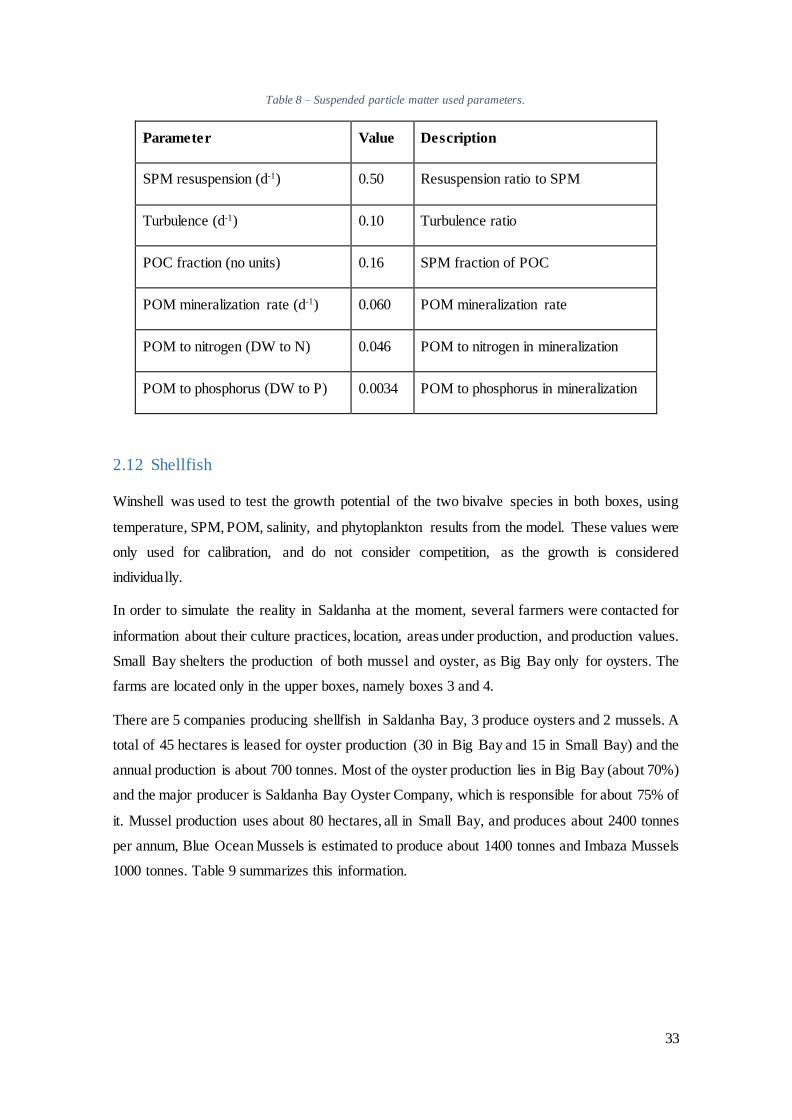
33

Table 8 – Suspended particle matter used parameters.

Parameter Value Description

SPM resuspension (d-1) 0.50 Resuspension ratio to SPM

Turbulence (d-1) 0.10 Turbulence ratio

POC fraction (no units) 0.16 SPM fraction of POC

POM mineralization rate (d-1) 0.060 POM mineralization rate

POM to nitrogen (DW to N) 0.046 POM to nitrogen in mineralization

POM to phosphorus (DW to P) 0.0034 POM to phosphorus in mineralization

2.12 Shellfish

Winshell was used to test the growth potential of the two bivalve species in both boxes, using

temperature, SPM, POM, salinity, and phytoplankton results from the model. These values were

only used for calibration, and do not consider competition, as the growth is considered

individually.

In order to simulate the reality in Saldanha at the moment, several farmers were contacted for

information about their culture practices, location, areas under production, and production values.

Small Bay shelters the production of both mussel and oyster, as Big Bay only for oysters. The

farms are located only in the upper boxes, namely boxes 3 and 4.

There are 5 companies producing shellfish in Saldanha Bay, 3 produce oysters and 2 mussels. A

total of 45 hectares is leased for oyster production (30 in Big Bay and 15 in Small Bay) and the

annual production is about 700 tonnes. Most of the oyster production lies in Big Bay (about 70%)

and the major producer is Saldanha Bay Oyster Company, which is responsible for about 75% of

it. Mussel production uses about 80 hectares, all in Small Bay, and produces about 2400 tonnes

per annum, Blue Ocean Mussels is estimated to produce about 1400 tonnes and Imbaza Mussels

1000 tonnes. Table 9 summarizes this information.

34

Table 9 – Companies working in Saldanha Bay, respective annual production and licensed area.

Company Product Location Area

(ha)

Annual production

(ton)

Oyster Saldanha Bay

Oyster Company

Small Bay and

Big Bay

35

(10 SB + 25 BB)

525

West Coast Big Bay 5 140

Blue Safire

Pearls

Small Bay 5 40

Total - - 45 705

Mussel Imbaza Mussels Small Bay 30 1000

Blue Ocean

Mussels

Small Bay 50 1000

Total - - 80 2000

Oysters are seeded with approximately 4 g, in both Bays, and mussel production uses mostly

natural seeding, which for modelling purposes was assumed to be around 0.65 g. Mussel weight

at harvest is between 25 and 40 g, and oysters around 70 g. Therefore the model is programed to

harvest mussels from 25 g and oysters from 61 g. The defined number of seeds for mussels was

50 million, for oysters around 2 million in Small Bay and 5 million in Big Bay. The information

provided for mortalities was assumed to be around 10% annually for both species. Table 10

resumes this information.

35

Table 10 – Mussel and oyster production, number of seeds, farm area, seed and harvested shellfish weight.

Shellfish Parameters Box 3 (Big

Bay)

Box 4 (Small

Bay)

Mussel Farm area (ha) - 80

Number of seeds - 50 million

Seed weight (g) - 0,65 g

Harvested weight (g) - 25 – 40 g

Oyster Farm area (ha) 30 15

Number of seeds 5 million 2 million

Seed weight (g) 4.3 4,3 g

Harvested weight (g) 70 70 g

36

37

3 Results and Discussion

3.1 Water temperature

Temperature in the Outer Bay is lower than in the remaining boxes, as it is more strongly under

the effect of the ocean circulation water. In the Outer Bay the temperature ranges between 11 ºC

and 15 ºC. The Big and Small Bay have a maximum of 18 ºC and a minimum 11 ºC. Langebaan

has the higher temperatures with a maximum of 20 ºC.

Figure 18 show’s temperature stratification during the summer period in all boxes except for

boxes 2 and 6, which is in agreement to what has been studied in Monteiro and Largier, (1999).

Water temperature in the upper boxes is higher during the summer, lower boxes show higher

values during the winter due to the break of the thermocline. Langebaan Lagoon has a more

homogeneous water temperature depth profile (less stratification) as the remaining areas. As such,

both boxes 2 and 6 have warmer water during the summer and colder in the winter.

The general presence of thermocline during the summer and mixture in the winter in all areas is

accordingly to the reality in the bay. The temperature range and the differences between boxes

seem also very acceptable.

Figure 18 – Temperature results for each box and measured data.

38

3.2 Salinity

Salinity shows an identical profile in all boxes, the lower values are observed in winter, minimum

of 34.7 and a maximum value of 35 psu in the spring. The average salinity is 34.8 psu.

Figure 19 – Salinity results for each box.

Salinity data is available to boxes 1, 3, 5, and 7, therefore, and as all boxes have very similar

results respecting salinity, only this boxes were tested. All boxes correlated strongly (r>0.945;

v=3) except box 3 (r=0.339; v=3). Even without correlation box 3 had identical mean salinity

values (34.80 psu against 34.78 measured) and showed a lower value during winter as measured

value, as the remaining boxes did. As a result all boxes seem to have acceptable salinity results.

3.3 Dissolved Inorganic Matter

The nutrient variable used for the phytoplankton growth is dissolved inorganic carbon (DIN), the

sum of NO2, NO3, and NO4, as such, these nutrients are analysed as DIN. The results obtained,

show a similar profile for all boxes, all boxes have a major peak in the winter with two smaller

peaks during summer. The average DIN is 4 µmol L-1, the maximum is 14 µmol L-1 and the

minimum value is close to 0 µmol L-1. Figure 20 illustrates DIN annual variation.

34,7

34,75

34,8

34,85

34,9

34,95

35

35,05

350 400 450 500 550 600 650 700

Sali

nit

y (p

su)

Julian day (d)

Box 1 Box 2 Box 3 Box 4

Box 5 Box 6 Box 7 Box 8

39

Figure 20 – DIN results for each box.

The only data available to test the nutrient results is the same used to insert them, and therefore

in station 1. Most boxes had average annual DIN close to the data used to build the model, except

for box 2 which had lower values. Table 11 illustrates the annual average DIN measured and

modelled for the different boxes.

Table 11 – Comparison between measured average DIN and mean DIN results for each box.

Box 1 Box 2 Box 3 Box 4 Upper layer Box 5 Box 6 Box 7 Box 8 Lower layer

DIN

(µg L-1)

3.4 0.75 2.63 2.22 2.6 6.5 6.9 6.5 4.9 7.6

Boxes 2 and 6, as expected, have different values from the remaining, because they have a very

distinct morphology and a weak connection to the remaining boxes. The observed DIN mean

value for each box is not too distant from the measured ones and the spatial variability within the

Bay is not known, so this shows only that this values are inside an acceptable range.

DIN may vary substantially and it is difficult to predict, due to the dynamics and communication

with the other objects, namely, phytoplankton and POM. These dynamics alter DIN in the water

column, which is consumed by phytoplankton and augmented by POM mineralization.

0

2

4

6

8

10

12

14

16

360 410 460 510 560 610 660 710 760

DIN

(u

mo

l L-1

)

Julian day (d)

Box 1 Box 2 Box 3 Box 4

Box 5 Box 6 Box 7 Box 8

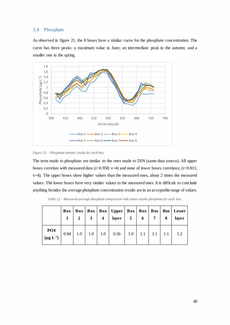
40

3.4 Phosphate

As observed in figure 21, the 8 boxes have a similar curve for the phosphate concentration. The

curve has three peaks: a maximum value in June; an intermediate peak in the autumn; and a

smaller one in the spring.

Figure 21 – Phosphate annual results for each box.

The tests made to phosphate are similar to the ones made to DIN (same data source). All upper

boxes correlate with measured data (r>0.958; v=4) and none of lower boxes correlates, (r<0.811;

v=4). The upper boxes show higher values than the measured ones, about 2 times the measured

values. The lower boxes have very similar values to the measured ones. It is difficult to conclude

anything besides the average phosphate concentration results are in an acceptable range of values.

Table 12 – Measured average phosphate comparison with mean results phosphate for each box.

Box

1

Box

2

Box

3

Box

4

Upper

layer

Box

5

Box

6

Box

7

Box

8

Lower

layer

PO4

(µg L-1) 0.84 1.0 1.0 1.0 0.56 1.0 1.1 1.1 1.1 1.2

0

0,2

0,4

0,6

0,8

1

1,2

1,4

1,6

1,8

360 410 460 510 560 610 660 710 760

Ph

osp

ha

te (

µg

L-1)

Julian day (d)

Box 1 Box 2 Box 3 Box 4

Box 5 Box 6 Box 7 Box 8

41

3.5 Suspended Particulate Matter

The SPM shows a relatively stable evolution across the year, with 4 small peaks occurring

approximately every 3 months. The maximum value is 32 mg L-1 the minimum 21 mg L-1 and the

average 26 mg L-1.

Figure 22 – SPM results for each box.

The only SPM data available is for a 10 day period, which is not sufficient to test SPM. Therefore

there can only be commented that SPM results are inside the data range, as the measured range

is: 9 to 61 mg L-1 and the results range is 21 to 32 mg L-1, which is acceptable.

19

21

23

25

27

29

31

33

350 400 450 500 550 600 650 700

SPM

(m

g L-1

)

Julian day (d)

Box 1 Box 2 Box 3 Box 4

Box 5 Box 6 Box 7 Box 8

42

3.6 Particulate Organic Matter

POM is stable during the year in all boxes. The lower ones show higher and similar values (around

1.8 mg L-1), except for box 5 that has an average value of 1.4 mg L-1. The upper boxes and box 5

have an average value of 1 mg L-1. The Figure below illustrates this.

Figure 23 – POM results for each box.

Data available to test POM is the same source as to SPM, with the same limitations. Avvailable

data ranges from 0.5 mg L-1 to 1.4 mg L-1 and the results show values between 0.9 mg L-1 and 1.9

mg L-1. POM is influenced by phytoplankton mortalities and by mineralization processes, whereby

these parameters adjustment could help to approximate the results to reality. However, the reality

will probably differ from the available data, as this is only existing for a short time period.

3.7 Phytoplankton

Phytoplankton biomass, shows major values in September, about 16 µg chl a L-1, and a small peak

in March. Only box 2 shows a slightly different profile, with higher values during the first months,

a major peak during winter and lower values in September. The average biomass is 7.5 µg Chl a

L-1 and the minimum is around 2 µg Chl a L-1. Figure 24 illustrates the described annual biomass

evolution.

0,7

0,9

1,1

1,3

1,5

1,7

1,9

2,1

350 400 450 500 550 600 650 700

PO

M (

mg

L-1)

Julian day (d)

Box 1 Box 2 Box 3 Box 4

Box 5 Box 6 Box 7 Box 8

43

Figure 24 – Phytoplankton results for each box.

Farms are located in boxes 3 and 4 (Big and Small Bay respectively) and therefore is important

to analyse them individually. The maximum value is 14 the minimum 3.2 and the average is 8.6

µg Chl a L-1. The two boxes have similar curves and values as Figure 25 illustrates.

Figure 25 – Phytoplankton results for boxes 3 and 4.

Several studies reported phytoplankton biomass in Saldanha Bay: Henry et al., (1977) and Pitcher

et al., (2015) found values between 5 and 32 mg chl a m-3, with a mean 15.5 mg chl a m-3; Smith

and Pitcher, (2015) and Pitcher and Calder, (1998) found a mean value of 8.6 mg chl a m-3.

Comparing the model results with these studies, they seem to be acceptable, with a mean value

of 7.5 mg chl a m-3, slightly lower than the results from Smith and Pitcher, (2015) and Pitcher

and Calder, (1998).

0

2

4

6

8

10

12

14

16

18

20

350 400 450 500 550 600 650 700

Ph

yto

pla

nkt

on

(ug

Ch

la L

-1)

Julian day (d)

Box 1 Box 2 Box 3 Box 4

Box 5 Box 6 Box 7 Box 8

0

2

4

6

8

10

12

14

16

350 400 450 500 550 600 650 700

Ph

yto

pla

nkt

on

(ug

Ch

la L

-1)

Julian day (d)

Box 3 Box 4

44

Smith and Pitcher, (2015) found that the phytoplankton biomass in Saldanha Bays is lower during

the winter months, and raises during the summer, with its maximum values in April. As it can be

observed in Figure 25, the results for phytoplankton biomass have its minimum in January, a

similar depression during the winter months, and a small peak in April, but the maximum biomass

happens in September. Pitcher and Calder, (1998), also had two similar peaks: one around April

and another around September, although the September peak was not the maximum biomass

along the year. Henry et al., (1977) also found a similar profile with one peak in April and another

in October.

The phytoplankton biomass results do not correlate with the available measured data, despite this

the curve profile is similar to the measured studies, showing the same cyclic peaks and

depressions. The total average chlorophyll in the data used to build the model is very close to the

one in results with a mean 7.8 mg chl a m-3.

The phytoplankton biomass correlates strongly for the same boxes (r>0.919; v=3) with boundary

values. Meaning that most of phytoplankton biomass in the model comes from the ocean, as

opposite to primary production inside of it.

3.8 Ecological model discussion

Phytoplankton biomass in the Bay is mostly limited by nutrients and light (Pitcher et al 1992).

The model is not completely accordingly to the reality, as phytoplankton seems to be mostly

dependent on exchanges with the boundaries, which happens mostly because of the system

morphology. This system parcelling in 8 big boxes simplifies much of the spatial variation,

meaning that at a given moment the value of each variable is homogeneous inside each box. This

will approximate the boundary effects on the more remote areas of the Bay, as the transport time

between these boxes and the boundary is shorter, and the maximum distance between them is one

of 2 boxes (for Langebaan area in particular). This explains why the variables correlate with the

boundary conditions more than with collected data, as its influence augmented with this

morphology.

It is difficult to evaluate whether the model describes the main ecological processes properly, as

the available data are not collected for this study and leave some uncertainty about their accuracy

for this study. However the results produced are within the range of expected values for all the

variables and show some acceptable temporal distribution. Most importantly the phytoplankton

results have an appropriate range of values and a profile that fits in the measured reality.

The absence of specific parameters for the relation of these variables, such as, the maximum

growth rate and optimum light for phytoplankton and the mineralization rates for POM, give some

room for adjustments.

45

3.9 Model validation – Standard Scenario

Estimated harvest is based on information provided by local farmers, mostly based on simple

estimations, the model was calibrated in order to obtain harvest results close to this estimations.

Estimated mussel production in Saldanha is about 2400 tonnes, the modelled harvest results have

approximately the same values. The oyster estimated production was about 520 tonnes for Big

Bay and 150 for Small Bay. The modelled results for oyster harvest are 510 tonnes for Big Bay

and 140 tonnes for Small Bay. Table 13 summarizes the expected and modelled harvest for each

box.

Table 13 – Modelled and estimated production for each box, organized in species.

Box 3 Box 4

Mussel annual production (ton) Estimated - 2400

Modelled - 2400

Oyster annual production (ton) Estimated 520 150

Modelled 510 140

Figure 26 shows the annual mussel and oyster harvest during 10 years of cultivation. The first

harvest year for mussels is year 3 with about 1700 tonnes, stabilizing in a mean 2400 tonnes on

the third harvested year. Oyster harvest starts in year 2 and it stabelizes in the second harvested

year (year 3) for both boxes. Box 3 produces considerably more as the number of seeds in it is

about 2.5 times bigger.

46

Figure 26 – Standard scenario harvested weight for each species for each area

Figure 27 shows the oyster individual weight in Winshell during one year (two charts on top) and

mussel individual weight (the one on the bottom). Box 4 produced bigger oysters, with 130 g and

125 g in box 3. Mussel individual weight was around 37 g after 13 months.

Figure 27 – Oyster individual weight evolution in box 3 (left side) box 4 (right side), mussel individual weight evolution

in box 4 (bottom)

Mussels individual weight is within the local farmers estimations: between 25 and 40 g; Oyster

individual weight is much above the estimated mean 80 g, about 30 g above it. Data introduced

in Winshell relative to Small Bay, was sligthtly higher in phytoplakton biomass compared to Big

Bay and therefore has heavier results.

0

500

1000

1500

2000

2500

3000

Y1 Y2 Y3 Y4 Y5 Y6 Y7 Y8 Y9 Y10

Ha

rves

ted

wei

ght

(to

n)

Year Nº

Oyster Big Bay Oyster Small Bay Mussel

47

Winshell does not considerate competition nor any group dynamics inside the box. Therefore, the

smaller dymensions and higher seeding in Small Bay facing Big Bay are not considered in

Winshell. Winshell results are merely used to test if the conditions inside the Bay alow the

shellfish to grow to the expected individual weight.

The change of a parameter such as POM mineralization may have substantial effects on the

bivalve growth rates in Winshell. The sensitivity analysis below (Figure 28) shows the variation

in mussel growth, the standard model with a mean POM concentration of 1.1 mg L-1, case 1 with

1.3 mg L-1 and case 3 with 0.9 mg L-1. This shows how a small variation of 0.2 mg L-1 in the mean

POM concentration can change the final weight with almost 20 g. Further calibration could

approximate the modelled individual weight to the real values.

Figure 28 – Oyster individual weight for 3 different POM scenarios: standard model (mean 1.1 mg L-1 POM); case 1

(mean 1.3 mg L-1 POM); case 2 (mean 0.9 mg L-1).

Winshell estimates system main uptakes and intakes. As the Table 13 illustrates, oyster production

removes about 1 tonnes Chla from the Bay per year as the mussel production removes circa 38

tonnes. Oyster production removes 106 tonnes POM per annum, circa 46 tonnes through

biodeposition, mussel production removes circa 6500 tonnes POM per annum, about half of it by

biodeposition. Oyster production removes circa 3 tonnes nitrogen per annum, and mussel

production removes circa 125 tonnes nitrogen.

0

20

40

60

80

100

120

140

0 50 100 150 200 250 300 350 400

Live

wei

ght

(g T

FW)

Time (d)

Live weight standard model Live weight case 1 Live weight case 2

48

Table 14 – Bivalve ecosystem removals for each farmed box.

Box 3 Box 4 Total oyster Total

Oyster Mussel Oyster

Phytoplankton (ton) 0.70 37.74 0.24 0.94 38.68

POM (ton) 106.0 6459.07 38.72 144.80 6603.87

POM Biodeposition (ton) 45.7 3399.17 17.12 62.84 3462.02

N (ton) 2.30 124.93 0.81 3.11 128.03

Mussel are responsible for about 99% of the calculated aquaculture removals in Saldanha Bay for

the referred parameters, this not only due to the higher mussel harvested weight. Considering the

removal per harvested weight, mussels remove circa 11 times more phytoplankton POM and N

as oysters do.

Figure 29 – Difference between phytoplankton biomass before and after adding shellfish farms to the model.

The introduction of shellfish into the model impacts the phytoplankton biomass, Figure 29 shows

the phytoplankton biomass results for each box before and after the farms introduction. The boxes

in which the difference is bigger are 4 and 8, followed by boxes 3 and 7. The impact in the

remaining boxes was not significant. The average phytoplankton biomass difference in box 4 is 3

mg chl a m-3, in box 8 1.2 mg chl a m-3, in box 1 only 0.5 mg chl a m-3 and in box 7 0.2 mg chl a

m-3.

0

2

4

6

8

10

12

Box 1 Box 2 Box 3 Box 4 Box 5 Box 6 Box 7 Box 8

Ph

yto

pla

nkt

on

bio

ma

ss (m

g ch

l am

3)

No farms Standard Scenario

49

Farms are located in boxes 3 and 4, but box 3 is about 3 times bigger in volume, and box 4 has

about 80% of the production. Box 4 is then submitted to a much bigger pressure than box 3 is.

This explains why the insertion of farms has greater impacts on phytoplankton biomass in box 4

and box 8 which is beneath it.

Table 15 – Mean phytoplankton comparison, before and after adding the farms into the model, in boxes 3, 4, 7, and

8.

Box 3 Box 4 Box 7 Box 8

Before farms

(mg chl a m-3)

8.57 8.52 5.82 5,56

After Farms (mg chl a m-3) 8.05 5.48 5.60 4.34

Difference (mg chl a m-3) 0.52 3.03 0.23 1.22

Table 14 illustrates the differences between the average phytoplankton biomass before and after

introducing the farms. As most of the analysed studies such as Pitcher et al. (2015), Pitcher and

Calder (1998), and Smith and Pitcher (2015) were made under the farms pressure on

phytoplankton, these values must match the measured ones. Pitcher and Calder, (1998) found

lower biomass in Small Bay, so the major difference obtained for these boxes is an expected

result.

The model allows to observe the farms influence in the ecosystem. Using Winshell individual

removals it is possible to make an estimation of the ecosystem services and some possible impacts

crated by the actual farming intensity. The current aquaculture activities may remove about 38

tonnes chlorophyll a, 126 tonnes nitrogen and 6500 tonnes POM. This improves water quality

and compensates for human nutrient inputs. Considering an annual emission of about 5 kg N per

capita (J and Drecht, 2004), and the populations of 21600 people of Saldanha and 8 000 in

Langebaan, this would represent an annual discharge of 148 tonnes N into the Bay and lagoon

area. The present seeding intensity potentially removes about 85% of human nitrogen water

inputs. Table 16 illustrates the total removals by each species.

50

Table 16 – Total scenario removal for each species and total

Mussels Oysters Total

Phytoplankton Removal (ton) 37 1 38

Nitrogen removal (ton) 123 3 126

Water clearance (m3) 6.02*109 1.29*108 6.15 *109

POM removal (ton) 6353 145 6497

POM biodeposition (ton) 3344 63 3406

3.10 Carrying capacity

3.10.1 Production carrying capacity

Saldanha’s Bay production carrying capacity is the maximum production that could be sustained

by the Bay. Using the interest of local scientists and farmers in production inside Small Bay,

production carrying capacity was determined for Small and Big Bay individually. Due to the

morphology of the Bay, and especially the model’s morphology, production in the Big Bay

influences significantly the food availability in Small Bay.

3.10.1.1 Small Bay

The production carrying capacity for Small Bay was calculated by maximizing the seeding for

both mussel and oyster individually. For both scenarios the remaining farms in Small and Big

Bay were not altered from the standard scenario seeding. Figure 30 illustrates the harvest obtained

for different seed intensities. The maximum production for mussel is about 5000 tonnes live

weight with seeding of about 145 tonnes. Oyster maximum production is about 20000 tonnes live

weight, with seeding of about 1100 tonnes. The Bay carrying capacity for oyster production is

considerably higher as for mussel, about the quadruple.

51

Figure 30 – Harvest results for different seeding intensities of mussel (left) and oyster (right), inside Small Bay

Seeds have different weight for the two species: the oyster is assumed to be 4.3 g and the mussel

0.65 g. Therefore, although the seeded oyster weight is superior, this is not directly comparable.

As Figure 31 shows, the number of seeds supported to obtain the maximum production in Small

Bay is also higher for oyster production.

Figure 31 – Number of seeds in Small Bay for the two maximum scenarios

Although oyster production is considerably higher than mussel production, in terms of meat

production they are not directly comparable. Oysters have big and heavy shells which constitute

about 70% of its live weight and mussels a smaller shell which represents only 40% of its live

weight. These estimations were carried out using Winshell average wet meat and shell weight

during the growth process of both species. As Figure 32 illustrates, oyster wet meat weight for

this scenario would be about 6000 tonnes and mussel would be about 3000 tonnes. Then the

maximum possible meat production would be achieved with oyster farms.

0

50

100

150

200

250

300

Mussel Oyster

Seed

nu

mb

er (

mil

lio

ns)

52

Figure 32 – Harvested shellfish in live weight and wet meat in tonnes for the maximum production scenarios in Small

Bay

The maximum production capacity, normally, is not the most profitable scenario. Harvested

shellfish have in this conditions lower growth rates and smaller shellfish have lower market value.

Higher seeding intensity have higher costs associated with seed purchase and farm maintenance

(Ferreira et al., 2007). Therefore the maximum production scenario is normally not the most

interesting one for farmers.

3.10.1.2 Big Bay

Big Bay maximum production capacity for oyster production was calculated similarly to Small

Bay. The seeding intensity was gradually raised in this box, and the remaining farms (in Small

Bay) were kept in the standard scenario level. As Figure 33 illustrates, the maximum production

for this Bay would be 100000 tonnes, with a seeded weight of about 4500 tonnes.

0

5000

10000

15000

20000

25000

Live weight Wet meat Live weight Wet meat

Mussel Oyster

Ha

rves

t (t

on

)

53

Figure 33 – Oyster harvested weight per seeded weight inside Big Bay

Determined oyster production capacity for Big Bay is compared with the oyster production

capacity for Small Bay in Figure 34. Calculated production capacity is circa 5 times higher in Big

Bay than in Small Bay. Big Bay is about 3 times bigger in area, so it would be expected to have

a higher capacity.

Figure 34 – Comparison of harvested live and wet meat weight of oyster in Small and in Big Bay.

0

20000

40000

60000

80000

100000

120000

0 1000 2000 3000 4000 5000 6000 7000

Oys

ter

ha

rves

t (to

n)

Seed (ton)

0

20000

40000

60000

80000

100000

120000

Live weight Wet meat Live weight Wet meat

Big bay Small bay

Oys

ter

Ha

rves

t (t

on

)

54

3.10.1.3 Small and Big Bay comparison

Small Bay production carrying capacity scenario would have significant impacts in phytoplankton

availability. As Figure 35 shows, phytoplankton biomass compared to standard scenario is

considerably lower in boxes 4 and 8, and almost unchanged for the remaining. Box 4 and 8 have

an average 2.5 and 3 mg chl a m-3, respectively.

The Big Bay production carrying capacity scenario would affect the entire Bay’s phytoplankton

availability. This is an expected output since this scenario introduces about the quadruple shellfish

inside the Bay and, as a consequence, has more phytoplankton uptake.

Figure 35 – Average phytoplankton biomass inside each box

When the two studied carrying capacity scenarios seeding intensities are used simultaneously, the

total harvested shellfish is less than the total obtained with Big Bay maximum production carrying

capacity alone.

0

2

4

6

8

10

12

Box 1 Box 2 Box 3 Box 4 Box 5 Box 6 Box 7 Box 8

Me

an

ph

ytop

lan

kton

bio

mas

s (m

g ch

la/m

3 )

Standard Model Small bay CC Big Bay CC

55

Figure 36 – Comparison of maximum production capacity in each box

3.11 Production scenarios:

After questioning local farmers and scientists, it was concluded that there is a bigger interest in

expand the cultures in Small Bay both for mussels and oyster. Therefore, two scenarios were built

and analysed for Small Bay: one increasing oyster production; and another mussel production.

3.11.1 Scenario 1

In this scenario the oyster seeding remained the same as in standard scenario, and the mussel

seeding was raised to a number 2 times bigger. In this scenario, the oyster production was not

affected by the mussel seeding raise and the mussel production stabilized with circa 5100 tonnes

per annum. The chart below shows this scenario harvest during the first 10 years.

Figure 37 – Scenario 2 annual shellfish harvest.

0

20000

40000

60000

80000

100000

120000

Small bay CC Big bay CC SB + BB CC

Shel

lfis

h h

arv

est (

ton

)

Big bay Small bay

0

500

1000

1500

2000

2500

3000

3500

4000

4500

Y1 Y2 Y3 Y4 Y5 Y6 Y7 Y8 Y9 Y10

Shel

lfis

h h

arv

est (

ton

)

Box 4 Oyster Box 4 Mussel Box 3 Oyster

56

3.11.2 Scenario 2

Oyster seeding in the Small Bay was raised to a number 100 times bigger as in standard scenario,

the oyster seeding in Big Bay and the mussel seeding was kept at the same intensity as in the

reference values. Oyster harvest in Big Bay was the same as in standard scenario, and the mussel

production diminished from 2400 tonnes to 2100. The oyster harvest in Small Bay raised to 14000

tonnes per year, as the chart below illustrates. The seeding intensity was raised till obtain a similar

chlorophyll profile.

Figure 38 – Scenario 2 oyster annual harvest in box 4.

3.11.3 Ecological impacts – Scenario 1 and 2

The two scenarios have very similar phytoplankton biomass distribution. A significant difference

in phytoplankton is observed in boxes 4 and 8, compared with the standard scenario. The chart

below illustrates this difference. The mean chlorophyll concentration during one year in box 4 is

37% lower than the standard scenario and in box 8, 19% lower. The remaining boxes have no

significant differences.

0

2000

4000

6000

8000

10000

12000

14000

16000

1 2 3 4 5 6 7 8 9 10

Shel

lfis

h h

arv

est (

ton

)

Box 4 Oyster Box 4 Mussel Box 3 Oyster

57

Figure 39 – Average phytoplankton biomass for each box and each scenario

Shellfish production in this scenarios would have great impacts on the water column. Accordingly

to WinShell results, scenario 1 would result in remoting circa 94 ton chl a from the water column

per year, circa 310 ton N and circa 16000 ton POM. Table 17 summarizes this information.

Table 17 – Scenario 4 ecological removals for each shellfish species.

Scenario 1 Scenario 2

Phytoplankton Removal (ton) 94 65

Nitrogen removal (ton) 310 216

Water clearance (m3) 1.5 *1010 9.8 * 109

POM removal (ton) 16027 10635

POM biodeposition (ton) 8421 5189

0

2

4

6

8

10

12

Box 1 Box 2 Box 3 Box 4 Box 5 Box 6 Box 7 Box 8

Ph

yto

pla

nkt

on

bio

mas

s (m

g ch

la/m

3)

Standard scenario Scenario 1 Scenario 2

58

3.12 Scenario discussion

Shellfish aquaculture may have positive effects in the Bay’s ecosystem when seeded in the correct

intensity. These removals may have an important role in compensating the nutrient inputs coming

from growth in waste water discharges, which is happening due to the population growth in

Saldanha and Langebaan. This top down control may be very important in preventing toxic algal

blooms, which benefits both aquaculture and fishing industry. Besides this, the phytoplankton

depletion will increase the underwater light availability, promoting the development of

submerged aquatic vegetation, which are important nursery sites for fish.

Biodeposition impacts over the farms may be significant in certain conditions, but this could only

be analysed at a farm scale with a different program. Further research and object development

would be necessary to observe the concrete impacts of different seeding intensities in the wild

shellfish species. The acceptable limit to ecological impact created by this activities is set by local

stakeholders and, therefore, may vary from site to site. The calculated maximum production

scenarios would most probably have considerable effects in the wild species by food competition,

since Sequeira et al., (2008) suggest that over-seeding may affect the benthic biodiversity through

food competition. This two scenarios result in a big reduction of phytoplankton biomass in the

water column. The oyster production involves seed purchase, and as such, the decrease in harvest

per seed weight is economically impacting for the farmers.

Scenarios 1 and 2 are interesting for farmers in Small Bay, as the production is increased without

significantly affecting bivalve growth rates. For the ecological perspective it is difficult to analyse

at what point the chlorophyll depletion would affect the wild filter feeders, without a previous

study to determine the wild life abundance, diversity and needs. Considering that farmed bivalves

growth rates are not significantly affected and that phytoplankton biomass decrease is lower in

box 8 (where the wild species would locate) it is reasonable to assume that the wild species

production would not be prejudiced.

The scenarios within this model give a system scale perspective, at which the competition for

food inside the farms is not considered, what may overestimate the results. For such detailed

analysis the use of another program such FARM would give a more local perspective. The

exclusion of the wild species competition may also condition the results and over-estimate the

farms harvest. Despite this the account for wild species would involve a different calibration of

the ecological model, and could still have similar results. Considering the uncertainty about most

of the parameters used in the ecological model, the use of different ones to consider these species

would be perfectly valid, and would probably be more close to the reality, since these animals are

part of the real ecosystem.

59

Scenario 2 production could present a sales volume of about 12 million euros. Which could have

positive social impacts in the community. According to Olivier et al., (2013) there is a relation of

89 employees for each 1000 tonnes shellfish produced. Which means this level of production

could employ 890 people, about 600 more people (assuming that now there are about 290 people

employed in the area, accordingly to the ratio).

In a future perspective, farmers could consider to participate in the nutrient credit trading market.

Given the potential removal of circa 310 ton N of scenario 1, this could represent an annual

income between 3 and 86 million euros, according to the tabled costs. These revenue represents

between 20 and 670% of the estimated sales volume, a significant amount for the farmers. Further

analysis would have to be carried out to determine whether there would be any use conflicts, or

impacts in local activities such fisheries, this could affect both social and physical carrying

capacity, and could determine a lower carrying capacity for the Bay.

60

61

4 Conclusion

This study main objectives were to: (1) describe Saldanha’s Bay main environmental variables

and its interaction with an aquaculture sector; (2) create different production scenarios; (3)

determine the system carrying capacity for shellfish production; and (4) to create a useful tool for

managing the Bay.

Saldanha Bay is a sheltered ecosystem northern from Cape Town in South Africa. This Bay is

part of the Benguela upwelling current system, providing a productive environment, with

excellent conditions for bivalve production. This system is home for several oyster and mussel

farms, with a total annual production of about 3000 tonnes.

This study made use of EcoWin, an object oriented program developed for modelling processes

in aquatic systems. The model incorporates a previously developed hydrodynamic model with a

biochemical model developed for northern Ireland, Belfast lough, in Ferreira et al. (2008). The

biochemical model was adapted for Saldanha Bay, using data collected by Probyn (Monteiro and

Largier, 1999; Smith and Pitcher, 2015). This system model includes many variables such as,

dissolved nutrients, particulate suspended matter, phytoplankton, shellfish, Man interaction, light,

salinity and water temperature. The farm component was developed using production methods

and other information provided by local producers after contacted.

The variables are dynamic and communicate with each other. Phytoplankton consumes nutrients,

and, through mortality, transforms into particle matter. Particulate organic matter decomposes

into nutrients. Shellfish consume both particulate organic matter and phytoplankton, they are also

harvested and seeded by Man object. Salinity, light and temperature influence way other variables

interact and its growth rates.

The model uses an 8 box system connected to the ocean, its only boundary. The biochemical

model uses suspended particulate matter, dissolved nutrients, salinity, all forced in the boundary.

Water temperature and light were forced for the entire system.

The results for all ecological variables are inside the respective, acceptable range of values. Mean

phytoplankton biomass is 7.5 mg chl a L-1, describing a curve with one major peak in September

and a smaller one in March. This against 8.6 mg chl a L-1 studied mean biomass is an acceptable

value.

After the addition of shellfish into the model, the phytoplankton biomass results kept an

acceptable mean 7 mg chl a L-1, with a biggest difference in box 4, where the most farms are

located. Pitcher and Calder, (1998) results show a lower phytoplankton biomass in Small Bay,

which means the lower values determined after introduction of shellfish area are adequate to the

reality.

62

The model simulates oyster growth with an average weight of 120 g and mussel with 35 g. The

annual harvest results are identical to the actual production, with a 2400 ton mussels and 140 ton

oyster in Small Bay, and about 510 tonnes in Big Bay. The oysters grow till 120 g in 365 days as

mussels reach 35 g in 395 days. The individual growth was much higher than the expected results,

which could be altered with further calibration of the model.

Production carrying capacity was determined individually for the Small Bay and Big Bay areas.

The Small Bay area had a maximum production capacity of about 5000 ton harvest for mussel

alone and 20000 tonnes for oyster alone. Big Bay area had the biggest production with about

100 000 ton oyster harvest. All the 3 scenarios were built from the standard scenario by raising

seeding intensities. These three scenarios were considered economically detrimental as it would

influence the shellfish size, lowering its market value. It is also not detrimental from the

environmental perspective, as it would probably also influence wild species growth result in

phytoplankton depletion, most likely impacting the wild bivalve species population inside the

affected areas.

The contacted local farmers showed interest in increasing production inside Small Bay and

therefore two scenarios were built. Scenario 1 raised mussel production and scenario 2 oyster

production, both inside Small Bay. Both scenario 1 and 2 raised the seeding intensity in Small

Bay comparing with standard model. Scenario 1 raised mussel production up to 5100 tonnes, and

scenario 2 raised oyster production up to 20 000 tonnes. These scenarios showed great economic

and environmental potential. The possible environmental impacts in the benthic community do

not seem to be significant, and there are several potential positive impacts: light availability to

benthic communities, toxic algal bloom prevention and nutrient removal.

This study accomplished all of its objectives, as it produced a model that successfully describes

the ecosystem main interactions, capable of simulating the ecosystem response to different inputs.

It produced several production scenarios and determined the carrying capacity for bivalve

production in the Bay. This model is a very powerful management tool, which can be used by

local decision makers to maximize the Bay social, economic and environmental components of

Saldanha Bay.

The academic nature of this work influenced availability of some resources, which could

potentiate the accuracy and value of the model to a higher level. The model was built using

available work, which did not cover for all the wanted accuracy.

The hydrodynamic model for this kind of study would ideally have a finer grid, providing a more

detailed spatial distribution and extra accuracy to the information produced. However, this model

had to be adapted from its original one year long construction to a less detailed 3 months long

one, being then used for simulating a one year period, losing some detail in the water circulation.

63

Data used was not collected with the purpose to be used in this study and therefore, for some

variables, the information available did not cover for the exact areas where it should. So, data was

adapted for the model requirements but did not achieve a desirable high accuracy level. Despite

this, data available was sufficient to build a strong analysis. The parameters used for ecological

processes were adapted from studies produced for other sites, since there were no studies for

Saldanha Bay specifically, which could also add strength to the model results if determined and

studied for this particular case.

For future developments, there are some aspects that could be developed and make this work

more valuable. It would be very interesting to integrate this work in a bigger project, where data

was collected for boundary conditions on particles, phytoplankton and nutrients, as for the

temperature in each box. It could also be included the development of the hydrodynamic model

in a finer grid and extent it to full year coverage, which would add some extra detail in spatial

distribution.

This study could also be enriched with the introduction of a wild zoobenthos component. This

would include the competition and interaction of wild species with the ecological variables, would

add some strength to the model, a more complete description of the ecosystem, and allow the

analysis of the impacts on the benthic environment, with which the farmed bivalves compete for

food.

The addition of zooplankton would also make this model stronger and allow an indirect analysis

of the impacts of aquaculture to higher trophic animals in the ecosystem. Zooplankton feds on

phytoplankton and is food for some fishes and higher trophic animals. As such depletion of

zooplankton can have high impacts on higher trophic fish and, consequently, the fishing industry.

This would also be a very interesting and more complete analysis to the ecological carrying

capacity of bivalve production in the Bay.

64

65

5 Bibliography

Aguilar-Manjarrez, J., McDaid Kapetsky, J., Soto, D., 2010. The potential of spatial planning tools to support the ecosystem approach to aquaculture, in: FAO Fisheries and Aquaculture Proceedings (FAO). Presented at the FAO/Rome Expert Workshop, Rome (Italy), 19-21 Nov 2008, FAO.

Anderson, R.J., Smit, A.J., Levitt, G.J., 1999. Upwelling and fish-factory waste as nitrogen sources for suspended cultivation of Gracilaria gracilis in Saldanha Bay, South Africa. Hydrobiologia 398-399, 455–462. doi:10.1023/A:1017095831356

Aypa, S.M., n.d. Mussel Culture.

Bacher, C., Duarte, P., Ferreira, J.G., Héral, M., Raillard, O., 1997. Assessment and comparison of the Marennes-Oléron Bay (France) and Carlingford Lough (Ireland) carrying capacity with ecosystem models. Aquat. Ecol. 31, 379–394. doi:10.1023/A:1009925228308

Bostock, J., McAndrew, B., Richards, R., Jauncey, K., Telfer, T., Lorenzen, K., Little, D., Ross, L., Handisyde, N., Gatward, I., Corner, R., 2010. Aquaculture: global status and trends. Philos. Trans. R. Soc. Lond. B Biol. Sci. 365, 2897–2912. doi:10.1098/rstb.2010.0170

Boyd, C.E., Tucker, C.S., 2012. Pond Aquaculture Water Quality Management. Springer Science & Business Media.

Brigolin, D., Maschio, G.D., Rampazzo, F., Giani, M., Pastres, R., 2009. An individual-based population dynamic model for estimating biomass yield and nutrient fluxes through an off-shore mussel (Mytilus galloprovincialis) farm. Estuar. Coast. Shelf Sci. 82, 365–376. doi:10.1016/j.ecss.2009.01.029

Britz, P.J., Lee, B., Botes, L., 2009. AISA 2009 aquaculture benchmarking survey: Primary production and markets. AISA report produced by Enviro-Fish Africa (Pty) Ltd.

Byron, C.J., Costa-Pierce, B., 2013. Carrying capacity tools for use in the implementation of an ecosystems approach to aquaculture. Site Sel. Carr. Capacit. Inland Coast. Aquac. 87–101.

Chamberlain, J., Fernandes, T.F., Read, P., Nickell, T.D., Davies, I.M., 2001. Impacts of biodeposits from suspended mussel (Mytilus edulis L.) culture on the surrounding surficial sediments. ICES J. Mar. Sci. J. Cons. 58, 411–416. doi:10.1006/jmsc.2000.1037

Clark, B.M., Tunley, K., Hutchings, K., Steffani, N., Turpie, J., Jurk, C., Gericke, J., 2012. Saldanha Bay and Langebaan Lagoon State of the Bay 2011 (Technical Report). Anchor Environmental Consultants, South Africa.

Cohen, J.E., 1995. How Many People Can the Earth Support? The Sciences 35, 18–23. doi:10.1002/j.2326-1951.1995.tb03209.x

Costa-Pierce, B.A., 2010. Sustainable Ecological Aquaculture Systems: The Need for a New Social Contract for Aquaculture Development. Mar. Technol. Soc. J. 44, 88–112. doi:10.4031/MTSJ.44.3.3

Crawford, C.M., Macleod, C.K.A., Mitchell, I.M., 2003. Effects of shellfish farming on the benthic environment. Aquaculture 224, 117–140. doi:10.1016/S0044-8486(03)00210-2

Davies, I.M., McLeod, D., 2003. Scoping study for research into the aquaculture (shellfish) carrying capacity of GB coastal waters. The Crown Estate. Final report.

Dowd, M., 2005. A bio-physical coastal ecosystem model for assessing environmental effects of marine bivalve aquaculture. Ecol. Model. 183, 323–346. doi:10.1016/j.ecolmodel.2004.08.018

66

Duarte, C.M., Holmer, M., Olsen, Y., Soto, D., Marbà, N., Guiu, J., Black, K., Karakassis, I., 2009. Will the Oceans Help Feed Humanity? BioScience 59, 967–976. doi:10.1525/bio.2009.59.11.8

Duarte, P., Meneses, R., Hawkins, A.J.S., Zhu, M., Fang, J., Grant, J., 2003. Mathematical modelling to assess the carrying capacity for multi-species culture within coastal waters. Ecol. Model. 168, 109–143. doi:10.1016/S0304-3800(03)00205-9

Ferreira, J.G., 1995. ECOWIN — an object-oriented ecological model for aquatic ecosystems. Ecol. Model. 79, 21–34. doi:10.1016/0304-3800(94)00033-E

Ferreira, J.G., Bricker, S.B., 2015. Goods and services of extensive aquaculture: shellfish culture and nutrient trading. Aquac. Int. 1–23. doi:10.1007/s10499-015-9949-9

Ferreira, J.G., Hawkins, A.J.S., Bricker, S.B., 2007. Management of productivity, environmental effects and profitability of shellfish aquaculture — the Farm Aquaculture Resource Management (FARM) model. Aquaculture 264, 160–174. doi:10.1016/j.aquaculture.2006.12.017

Ferreira, J.G., Hawkins, A.J.S., Monteiro, P., Moore, H., Service, M., Pascoe, P.L., Ramos, L., Sequeira, A., 2008. Integrated assessment of ecosystem-scale carrying capacity in shellfish growing areas. Aquaculture 275, 138–151. doi:10.1016/j.aquaculture.2007.12.018

Figueras, A., 2004. Cultured Aquatic Species Information Programme Mytilus galloprovincialis.

Filgueira, R., Guyondet, T., Comeau, L.A., Grant, J., 2014. A fully-spatial ecosystem-DEB model of oyster (Crassostrea virginica) carrying capacity in the Richibucto Estuary, Eastern Canada. J. Mar. Syst. 136, 42–54. doi:10.1016/j.jmarsys.2014.03.015

Flemming, B.W., 1977. Depositional processes in Saldanha Bay and Langebaan Lagoon, CSIR Research Report 362 (revised edition, 2015). National Researchly Institute for Oceanology, Stellenbosch, South Africa.

Franco, A.R., Ferreira, J.G., Nobre, A.M., 2006. Development of a growth model for penaeid shrimp. Aquaculture 259, 268–277. doi:10.1016/j.aquaculture.2006.05.051

Garrido-Handog, L., n.d. Oyster Culture.

Gibbs, M.T., 2007. Sustainability performance indicators for suspended bivalve aquaculture activities. Ecol. Indic. 7, 94–107. doi:10.1016/j.ecolind.2005.10.004

Gibbs, M.T., 2004. Interactions between bivalve shellfish farms and fishery resources. Aquaculture 240, 267–296. doi:10.1016/j.aquaculture.2004.06.038

G.J., I., B.J., H., A.H., R., 2000. An Overview of Factors Affecting the Carrying Capacity of Coastal Embayments for Mussel Culture.

Gosling, E., 2008. Bivalve Molluscs: Biology, Ecology and Culture. John Wiley & Sons.

Grant, J., Hatcher, A., Scott, D.B., Pocklington, P., Schafer, C.T., Winters, G.V., 1995. A multidisciplinary approach to evaluating impacts of shellfish aquaculture on benthic communities. Estuaries 18, 124–144. doi:10.2307/1352288

Grant, J., Stenton-Dozey, J., Monteiro, P., Pitcher, G., Heasman, K., 1998. Shellfish mariculture in the Benguela system: a carbon budget of Saldanha Bay for raft culture of Mytilus galloprovincialis.

Guyondet, T., Roy, S., Koutitonsky, V.G., Grant, J., Tita, G., 2010. Integrating multiple spatial scales in the carrying capacity assessment of a coastal ecosystem for bivalve aquaculture. J. Sea Res. 64, 341–359. doi:10.1016/j.seares.2010.05.003

Handbook of Fishery Statistical Standards., FAO.

67

Harris, T.F.W., 1978. Review of Coastal Currents in Southern African Waters. Prepared for: South African National Comettee for Oceanographic Research and Comittee on Marine Pollution, South Africa.

Haven, D.S., Morales-Alamo, R., 1972. Biodeposition as a Factor in Sedimentation of Fine Suspended Solids in Estuaries. Geol. Soc. Am. Mem. 133, 121–130. doi:10.1130/MEM133-p121

Haven, D.S., Morales-Alamo, R., 1966. Aspects of Biodeposition by Oysters and Other Invertebrate Filter Feeders1. Limnol. Oceanogr. 11, 487–498. doi:10.4319/lo.1966.11.4.0487

Helm, M.M., 2005. Cultured Aquatic Species Information Programme. Crassostrea gigas. FAO Fish. Aquac. Dep. Online.

Helm, M.M., Bourne, N., Lovatelli, A., 2004. Hatchery culture of bivalves: a practical manual. Food and agriculture organization of the United Nations.

Henry, J.L., Mostert, S.A., Christie, N.D., 1977. Phytoplankton Production in Langebaan Lagoon and Saldanha Bay. Trans. R. Soc. South Afr. 42, 383–398. doi:10.1080/00359197709519923

James, R., F., Sokal, R.R., 1995. Statistical tables. Macmillan.

Jiang, W., Gibbs, M.T., 2005. Predicting the carrying capacity of bivalve shellfish culture using a steady, linear food web model. Aquaculture 244, 171–185. doi:10.1016/j.aquaculture.2004.11.050

J, K., Drecht, G. van, 2004. Global assessment of nitrogen inputs from point sources to surface water for the period 1970-2030.

Kaspar, H.F., Gillespie, P.A., Boyer, I.C., MacKenzie, A.L., 1985. Effects of mussel aquaculture on the nitrogen cycle and benthic communities in Kenepuru Sound, Marlborough Sounds, New Zealand. Mar. Biol. 85, 127–136. doi:10.1007/BF00397431

Kruger, A.C., Goliger, A.M., Retief, J.V., Sekele, S., 2010. Strong wind climatic zones in South Africa.

Lam, P.J., Bishop, J.K.B., 2007. High biomass, low export regimes in the Southern Ocean. Deep Sea Res. Part II Top. Stud. Oceanogr., The Role of Marine Organic Carbon and Calcite Fluxes in Driving Global Climate Change, Past and Future 54, 601–638. doi:10.1016/j.dsr2.2007.01.013

Luo, J., Hartman, K.J., Brandt, S.B., Cerco, C.F., Rippetoe, T.H., 2001. A Spatially-Explicit Approach for Estimating Carrying Capacity: An Application for the Atlantic Menhaden (Brevoortia tyrannus) in Chesapeake Bay. Estuaries 24, 545–556. doi:10.2307/1353256

McKindsey, C.W., Archambault, P., Callier, M.D., Olivier, F., 2011. Influence of suspended and off-bottom mussel culture on the sea bottom and benthic habitats: a review1This review is part of a virtual symposium on current topics in aquaculture of marine fish and shellfish. Can. J. Zool. 89, 622–646. doi:10.1139/z11-037

McKindsey, C.W., Thetmeyer, H., Landry, T., Silvert, W., 2006. Review of recent carrying capacity models for bivalve culture and recommendations for research and management. Aquaculture 261, 451–462. doi:10.1016/j.aquaculture.2006.06.044

McLeod, I., Pantus, F., Preston, N., 2002. The use of a geographical information system for land-based aquaculture planning. Aquac. Res. 33, 241–250. doi:10.1046/j.1355-557x.2001.00667.x

Monteiro, P.M.S., Brundrit, G.B., 1990. Interannual chlorophyll variability in South Africa’s Saldanha Bay system, 1974–1979. South Afr. J. Mar. Sci. 9, 281–287. doi:10.2989/025776190784378899

68

Monteiro, P.M.S., Largier, J.L., 1999. Thermal Stratification in Saldanha Bay (South Africa) and Subtidal, Density-driven Exchange with the Coastal Waters of the Benguela Upwelling System. Estuar. Coast. Shelf Sci. 49, 877–890. doi:10.1006/ecss.1999.0550

Olivier, D., Heinecken, L., Jackson, S., 2013. Mussel and oyster culture in Saldanha Bay, South Africa: potential for sustainable growth, development and employment creation. Food Secur. 5, 251–267. doi:10.1007/s12571-013-0244-1

Pauley, G.B., Van Der Raay, B., Troutt, D., 1988. Species Profiles: Life Histories and Environmental Requirements of Coastal Fishes and Invertebrates (Pacific Northwest), Pacific Oyster.

Pitcher, G.C., Calder, D., 1998. Shellfish mariculture in the Benguela System: phytoplankton and the availability of food for commercial mussel farms in Saldanha Bay. J. Shellfish Res.

Pitcher, G.C., Krock, B., Cembella, A.D., 2011. Accumulation of diarrhetic shellfish poisoning toxins in the oyster Crassostrea gigas and the mussel Choromytilus meridionalis in the southern Benguela ecosystem. Afr. J. Mar. Sci. 33, 273–281. doi:10.2989/1814232X.2011.600372

Pitcher, G., Smith, M., Probyn, T., 2015. Saldanha Bay, estimating bay productivity.

Probyn, T.A., Pitcher, G.C., Monteiro, P.M.S., Boyd, A.J., Nelson, G., 2000. Physical processes contributing to harmful algal blooms in Saldanha Bay, South Africa. South Afr. J. Mar. Sci. 22, 285–297. doi:10.2989/025776100784125807

Probyn, T., Pitcher, G., Pienaar, R., Nuzzi, R., 2001. Brown Tides and Mariculture in Saldanha Bay, South Africa. Mar. Pollut. Bull. 42, 405–408. doi:10.1016/S0025-326X(00)00170-3

Ross, L.G., Telfer, T.C., Falconer, L., Soto, D., Aguilar-Manjarrez, J., Asmah, R., Bermúdez, J., Beveridge, M.C.M., Byron, C.J., Clément, A., Richard Corner, Barry A. Costa-Pierce, Stephen F. Cross, Martin De Wit, Shaunglin Dong, João Gomes Ferreira, James McDaid Kapetsky, Ioannis Karakassis, William Leschen, David C. Little, Anne-Katrine Lundebye-Haldorsen, Francis J. Murray, Michael Phillips, Laudemira Ramos, Sherif Sadek, Philip C. Scott, Arnoldo Valle-Levinson, Douglas Waley, Patrick G. White, Changbo Zhu, 2013. Carrying capacities and site selection within the ecosystem approach to aquaculture. Site Sel. Carr. Capacit. Inland Coast. Aquac. 19.

Sequeira, A., Ferreira, J.G., Hawkins, A.J.S., Nobre, A., Lourenço, P., Zhang, X.L., Yan, X., Nickell, T., 2008. Trade-offs between shellfish aquaculture and benthic biodiversity: A modelling approach for sustainable management. Aquaculture 274, 313–328. doi:10.1016/j.aquaculture.2007.10.054

Shumway, S.E., Davis, C., Downey, R., Karney, R., Kraeuter, J., n.d. Guest Editorial Shellfish aquaculture — In praise of sustainable economies and environments.

Smaal, A.C., Prins, T.C., Dankers, N., Ball, B., 1997. Minimum requirements for modelling bivalve carrying capacity. Aquat. Ecol. 31, 423–428. doi:10.1023/A:1009947627828

Smith, M., Pitcher, G., 2015. Saldanha Bay South Africa: the use of ocean colour remote sensing to assess phytoplankton biomass.

Souchu, P., Vaquer a, A., Collos, Y., Landrein, S., Deslous-Paoli, J.-M., Bibent, B., 2001. Influence of shellfish farming activities on the biogeochemical composition of the water column in Thau lagoon. Mar. Ecol. Prog. Ser. 218, 141–152.

Steele, J.H., 1962. Environmental Control of Photosynthesis in the Sea. Limnol. Oceanogr. 7, 137–150. doi:10.4319/lo.1962.7.2.0137

Stenton-dozey, J.M.E., Jackson, L.F., Busby, A.J., 1999. Impact of Mussel Culture on Macrobenthic Community Structure in Saldanha Bay, South Africa. Mar. Pollut. Bull. 39, 357–366. doi:10.1016/S0025-326X(98)00180-5

69

Stenton-Dozey, J., Probyn, T., Busby, A., 2001. Impact of mussel (mytilus galloprovincialis) raft-culture on benthic macrofauna, in situ oxygen uptake, and nutrient fluxes in Saldanha Bay, South Africa. Can. J. Fish. Aquat. Sci. 58, 1021.

Strohmeier, T., Duinker, A., Strand, Ø., Aure, J., 2008. Temporal and spatial variation in food availability and meat ratio in a longline mussel farm (Mytilus edulis). Aquaculture 276, 83–90. doi:10.1016/j.aquaculture.2008.01.043

United Nations, 2015. World population projected to reach 9.7 billion by 2050 | UN DESA | United Nations Department of Economic and Social Affairs.

Wit, M., 2013. Aquaculture in Southern Africa with special reference to site selection and carrying capacity issues. Site Sel. Carr. Capacit. Inland Coast. Aquac. 207.

Zhang, J., Hansen, P.K., Fang, J., Wang, W., Jiang, Z., 2009. Assessment of the local environmental impact of intensive marine shellfish and seaweed farming—Application of the MOM system in the Sungo Bay, China. Aquaculture 287, 304–310. doi:10.1016/j.aquaculture.2008.10.008