Survival of Dominated Strategiesunder Evolutionary Dynamics∗

Josef Hofbauer† and William H. Sandholm‡

September 27, 2010

Abstract

We prove that any deterministic evolutionary dynamic satisfying four mild re-quirements fails to eliminate strictly dominated strategies in some games. We alsoshow that existing elimination results for evolutionary dynamics are not robust tosmall changes in the specifications of the dynamics. Numerical analysis reveals thatdominated strategies can persist at nontrivial frequencies even when the level of dom-ination is not small.

1. Introduction

One fundamental issue in evolutionary game theory concerns the relationship betweenits predictions and those provided by traditional, rationality-based solution concepts.Indeed, much of the early interest in the theory among economists is due to its ability tojustify traditional equilibrium predictions as consequences of myopic decisions made bysimple agents.

Some of the best known results in this vein link the rest points of a deterministicevolutionary dynamic with the Nash equilibria of the game being played. Under mostdynamics considered in the literature, the set of rest points includes all Nash equilibria of

∗We thank Drew Fudenberg, Larry Samuelson, a number of anonymous referees, a co-editor, and manyseminar audiences for helpful comments, and Emin Dokumacı for outstanding research assistance. Manyfigures in this article were created using the Dynamo open-source software suite (Sandholm and Dokumacı(2007)). Financial support from NSF Grants SES-0092145, SES-0617753, and SES-0851580, the Centre forEconomic Learning and Social Evolution (ELSE) at University College London, and the University ofVienna is gratefully acknowledged.†Department of Mathematics, University of Vienna, Nordbergstrasse 15, A-1090 Vienna, Austria. e-mail:

josef.hofbauer@univie.ac.at; website: http://homepage.univie.ac.at/josef.hofbauer.‡Department of Economics, University of Wisconsin, 1180 Observatory Drive, Madison, WI 53706, USA.

e-mail: whs@ssc.wisc.edu; website: http://www.ssc.wisc.edu/∼whs.

the underlying game, and under many of these dynamics the sets of rest points and Nashequilibria are identical.1

In order to improve upon these results, one might look for dynamics that convergeto Nash equilibrium from most initial conditions regardless of the game at hand. Such afinding would provide a strong defense of the Nash prediction, as agents who began playat some disequilibrium state could be expected to find their way to Nash equilibrium.Unfortunately, results of this kind cannot be proved. Hofbauer and Swinkels (1996) andHart and Mas-Colell (2003) show that no reasonable evolutionary dynamic converges toNash equilibrium in all games: there are some games in which cycling or more complicatedlimit behavior far from any Nash equilibrium is the only plausible long run prediction.

These negative results lead us to consider a more modest question. Rather than seekevolutionary support for equilibrium play, we instead turn our attention to a more basicrationality requirement: namely, the avoidance of strategies that are strictly dominatedby a pure strategy.

Research on this question to date has led to a number of positive results. Two of thecanonical evolutionary dynamics are known to eliminate strictly dominated strategies,at least from most initial conditions. Akin (1980) shows that starting from any interiorpopulation state, the replicator dynamic (Taylor and Jonker (1978)) eliminates strategiesthat are strictly dominated by a pure strategy. Samuelson and Zhang (1992), buildingon work of Nachbar (1990), extend this result to a broad class of evolutionary dynamicsdriven by imitation: namely, dynamics under which strategies’ percentage growth ratesare ordered by their payoffs.2 Elimination results are also available for dynamics basedon traditional choice criteria: the best response dynamic (Gilboa and Matsui (1991))eliminates strictly dominated strategies by construction, as under this dynamic revisingagents always switch to optimal strategies. Since the elimination of strategies strictlydominated by a pure strategy is the mildest requirement employed in standard game-theoretic analyses, it may seem unsurprising that two basic evolutionary dynamics obeythis dictum.

In this paper, we argue that evolutionary support for the elimination of dominatedstrategies is more tenuous than the results noted above suggest. In particular, we provethat all evolutionary dynamics satisfying four mild conditions—continuity, positive cor-relation, Nash stationarity, and innovation—must fail to eliminate strictly dominatedstrategies in some games. Dynamics satisfying these conditions include not only well-

1For results of the latter sort, see Brown and von Neumann (1950), Smith (1984), and Sandholm (2005,2010a).

2Samuelson and Zhang (1992) and Hofbauer and Weibull (1996) also introduce classes of imitativedynamics under which strategies strictly dominated by a mixed strategy are eliminated.

–2–

known dynamics from the evolutionary literature, but also slight modifications of thedynamics under which elimination is known to occur. In effect, this paper shows that thedynamics known to eliminate strictly dominated strategies in all games are the only onesone should expect to do so, and that even these elimination results are knife-edge cases.

An important predecessor of this study is the work of Berger and Hofbauer (2006),who present a game in which a strictly dominated strategy survives under the Brown-vonNeumann-Nash (BNN) dynamic (Brown and von Neumann (1950)). We begin the presentstudy by showing how Berger and Hofbauer’s (2006) analysis can be extended to a varietyof other dynamics, including the Smith dynamic (Smith (1984)) as well as generalizationsof both the BNN and Smith dynamics (Hofbauer (2000), Sandholm (2005, 2010a)). Whilethis analysis is relatively simple, it is not general, as it depends on the functional formsof the dynamics at issue. Since in practice it is difficult to know exactly how agents willupdate their choices over time, a more compelling elimination result would require onlyminimal structure.

Our main theorem provides such a result. Rather than specifying functional formsfor the evolutionary dynamics under consideration, the theorem allows for any dynamicsatisfying four mild conditions. The first, continuity, asks that the dynamic change con-tinuously as a function of the payoff vector and the population state. The second, positivecorrelation, is a weak montonicity condition: it demands that away from equilibrium, thecorrelation between strategies’ payoffs and growth rates always be positive. The third con-dition, Nash stationarity, asks that states that are not Nash equilibria—that is, states wherepayoff improvement opportunities are available—are not rest points of the dynamic. Thefinal condition, innovation, is a requirement that has force only at non-Nash boundarystates: if at such a state some unused strategy is a best response, the growth rate of thisstrategy must be positive. The last two conditions rule out the replicator dynamic andthe other purely imitative dynamics noted above; at the same time, they allow arbitrarilyclose approximations of these dynamics, under which agents usually imitate successfulopponents, but occasionally select new strategies directly.

To prove the main theorem, we construct a four-strategy game in which one strategy isstrictly dominated by another pure strategy. We show that under any dynamic satisfyingour four conditions, the strictly dominated strategy survives along solution trajectoriesstarting from most initial conditions.

Because evolutionary dynamics are defined by nonlinear differential equations, ourformal results rely on topological properties, and so provide limited quantitative infor-mation about the conditions under which dominated strategies survive. We thereforesupplement our formal approach with numerical analysis. This analysis reveals that

–3–

dominated strategies with payoffs substantially lower than those of their dominatingstrategies can be played at nontrivial frequencies in perpetuity.

Since elimination of dominated strategies is a basic requirement of traditional gametheory, the fact that such strategies can persist under evolutionary dynamics may seemcounterintuitive. A partial resolution of this puzzle lies in the fact that survival of domi-nated strategies is intrinsically a disequilibrium phenomenon.

To understand this point, remember that evolutionary dynamics capture the aggregatebehavior of agents who follow simple myopic rules. These rules lead agents to switch tostrategies whose current payoffs are good, though not necessarily optimal.

When a solution trajectory of an evolutionary dynamic converges, the payoffs to eachstrategy converge as well. Because payoffs become fixed, even simple rules are enough toensure that only optimal strategies are chosen. In formal terms, the limits of convergentsolution trajectories must be Nash equilibria; it follows a fortiori that when these limits arereached, strictly dominated strategies are not chosen.

Of course, it is well understood that solutions of evolutionary dynamics need notconverge, but instead may enter limit cycles or more complicated limit sets.3 When solu-tions do not converge, payoffs remain in flux. In this situation, it is not obvious whetherchoice rules favoring strategies whose current payoffs are relatively high will necessarilyeliminate strategies that perform well at many states, but that are never optimal. To thecontrary, the analysis in this paper demonstrates that if play remains in disequilibrium,even strategies that are strictly dominated by other pure strategies can persist indefinitely.

One possible reaction to our results is to view them as an argument against the rele-vance of evolutionary dynamics for modeling economic behavior. If an agent notices thata strategy is strictly dominated, then he would do well to avoid playing it, whatever hisrule of thumb might suggest. We agree with the latter sentiment: we do not expect agents,even simple ones, to play strategies they know to be dominated. At the same time, wefeel that the ability to recognize dominated strategies should not be taken for granted. Incomplicated games with large numbers of participants, it may not always be reasonableto expect agents to know the payoffs to all strategies at every population state, or to beable to make all the comparisons needed to identify a dominated strategy. It is precisely insuch large, complex games that agents might be expected to make decisions by applyingrules of thumb. Our analysis suggests that if agents cannot directly exclude dominatedstrategies from their repertoire of choices, then these strategies need not fade from usethrough a lack of positive reinforcement.

3For specific nonconvergence results, see Shapley (1964), Jordan (1993), Gaunersdorfer and Hofbauer(1995), Hofbauer and Swinkels (1996), Hart and Mas-Colell (2003), and Sparrow et al. (2008); see Sandholm(2009a) for a survey.

–4–

To prove our main result, we must show that for each member of a large class ofdeterministic evolutionary dynamics, there is a game in which dominated strategies sur-vive. To accomplish this most directly, we use the same construction for all dynamicsin the class. We begin by introducing a three-strategy game with nonlinear payoffs—thehypnodisk game—under which solution trajectories of all dynamics in the class enter cyclesfrom almost all initial conditions. We then modify this game by adding a dominatedfourth strategy, and show that the proportion of the population playing this strategy staysbounded away from zero along solutions starting from most initial conditions.

Since the game we construct to ensure cyclical behavior is rather unusual, one mightwonder whether our survival results are of practical relevance, rather than being a mereartifact of a pathological construction. In fact, while introducing a special game is quiteconvenient for proving the main result, we feel that our basic message—that in the absenceof convergence, myopic heuristics need not root out dominated strategies in large games—is of broader relevance. In Section 5.1, we explain why the proof of the main theorem doesnot depend on the introduction of a complicated game in an essential way. Analyses thereand elsewhere in the paper suggest that in any game for which some dynamic covered bythe theorem fails to converge, there are augmented games with dominated strategies thatthe dynamic allows to survive.

Section 2 introduces population games and evolutionary dynamics. Section 3 estab-lishes the survival results for excess payoff dynamics and pairwise comparison dynamics,families that contain the BNN and Smith dynamics, respectively. Section 4 states andproves the main result. Section 5 presents our numerical analyses, and illustrates the sen-sitivity of existing elimination results to slight modifications of the dynamics in question.Section 6 concludes. Auxiliary results and proofs omitted from the text are provided inthe Appendix.

2. The Model

2.1 Population Games

We consider games played by a single unit mass population of agents.4 All agentschoose from the finite set of strategies S = {1, . . . ,n}. The set of population states istherefore the simplex X = {x ∈ Rn

+ :∑

i∈S xi = 1}, where xi is the proportion of agentschoosing strategy i ∈ S. The standard basis vector ei ∈ Rn represents the state at which allagents choose strategy i.

4Versions of our results can also be proved in multipopulation models.

–5–

If we take the set of strategies as fixed, we can identify a game with a Lipschitzcontinuous payoff function F : X → Rn, which assigns each population state x ∈ X a vectorof payoffs F(x) ∈ Rn. The component Fi : X → R represents the payoffs to strategy ialone. We also let F(x) =

∑i∈S xiFi(x) denote the population’s average payoff, and let

BF(x) = argmaxy∈X y′F(x) denote the set of (mixed) best responses at population state x.The simplest examples of population games are generated by random matching in

symmetric normal form games. An n-strategy symmetric normal form game is definedby a payoff matrix A ∈ Rn×n. Ai j is the payoff a player obtains when he chooses strategy iand his opponent chooses strategy j; this payoff does not depend on whether the playerin question is called player 1 or player 2. When agents are randomly matched to play thisgame, the (expected) payoff to strategy i at population state is x is Fi(x) =

∑j∈S Ai jx j; hence,

the population game associated with A is the linear game F(x) = Ax.While random matching generates population games with linear payoffs, many pop-

ulation games that arise in applications have payoffs that are nonlinear in the populationstate—see Section 5.1. Games with nonlinear payoff functions will play a leading role inthe analysis to come.

2.2 Evolutionary Dynamics

An evolutionary dynamic assigns each population game F an ordinary differentialequation x = VF(x) on the simplex X. One simple and general way of defining anevolutionary dynamic is via a growth rate function g : Rn

×X→ Rn; here gi(π, x) representsthe (absolute) growth rate of strategy i as a function of the current payoff vector π ∈ Rn

and the current population state x ∈ X. Our notation suppresses the dependence of g onthe number of strategies n.

To ensure that the simplex is forward invariant under the induced differential equa-tions, the function g must satisfy

gi(π, x) ≥ 0 whenever xi = 0, and∑i∈S

gi(π, x) = 0.

In words: strategies that are currently unused cannot become less common, and the sumof all strategies’ growth rates must equal zero. A growth rate function g satisfying theseconditions defines an evolutionary dynamic as follows:

xi = VFi (x) = gi(F(x), x).

One can also build evolutionary dynamics from a more structured model that not

–6–

Revision protocol Evolutionary dynamic Name Origin

ρi j = x j[F j − Fi]+ xi = xi(Fi(x) − F(x)) replicatorTaylor and

Jonker (1978)

ρi j = BFj (x) x ∈ BF(x) − x best response

Gilboa andMatsui (1991)

ρi j = [F j − F]+

xi = [Fi(x) − F(x)]+

−xi∑j∈S

[F j(x) − F(x)]+BNN Brown and von

Neumann (1950)

ρi j = [F j − Fi]+

xi =∑j∈S

x j[Fi(x) − F j(x)]+

−xi∑j∈S

[F j(x) − Fi(x)]+

Smith Smith (1984)

Table I: Four evolutionary dynamics and their revision protocols.

only provides explicit microfoundations for the dynamics, but also is inclusive enoughto encompass all dynamics considered in the literature.5 In this model, the growth ratefunction g is replaced by a revision protocol ρ : Rn

×X→ Rn×n+ , which describes the process

through which individual agents make decisions. As time passes, agents are chosen atrandom from the population and granted opportunities to switch strategies. When an iplayer receives such an opportunity, he switches to strategy j with probability proportionalto the conditional switch rate ρi j(π, x). Aggregate behavior in the game F is then describedby the differential equation

(1) xi = VFi (x) =

∑j∈S

x jρ ji(F(x), x) − xi

∑j∈S

ρi j(F(x), x),

which is known as the mean dynamic generated by ρ and F. The first term in (1) capturesthe inflow of agents into strategy i from other strategies, while the second term capturesthe outflow of agents from strategy i to other strategies.

Table I presents four basic examples of evolutionary dynamics, along with revisionprotocols that generate them. Further discussion of these dynamics can be found inSections 3.1, 5.3, and 5.4 below.

5For explicit accounts of microfoundations, see Benaım and Weibull (2003) and Sandholm (2003).

–7–

3. Survival under the BNN, Smith, and Related Dynamics

Using a somewhat informal analysis, Berger and Hofbauer (2006) argue that strictlydominated strategies can survive under the BNN dynamic (Brown and von Neumann(1950)). To prepare for our main result, we formalize and extend Berger and Hofbauer’s(2006) arguments to prove a survival result for two families of evolutionary dynamics;these families include the BNN dynamic and the Smith dynamic (Smith (1984)) as theirsimplest members.

3.1 Excess Payoff Dynamics and Pairwise Comparison Dynamics

The two families of dynamics we consider are based on revision protocols of the forms

ρi j = φ(F j − F) and(2)

ρi j = φ(F j − Fi),(3)

where in each case, φ : R→ R+ is a Lipschitz continuous function satisfying

(4) sgn(φ(u)) = sgn([u]+) and ddu+ φ(u)

∣∣∣u=0

> 0.

The families of evolutionary dynamics obtained by substituting expressions (2) and (3) intothe mean dynamic (1) are called excess payoff dynamics (Weibull (1996); Hofbauer (2000);Sandholm (2005)) and pairwise comparison dynamics (Sandholm (2010a)), respectively. TheBNN and Smith dynamics are the prototypical members of these two families: examiningTable I, we see that these two dynamics are those obtained from protocols (2) and (3) whenφ is the semilinear function φ(u) = [u]+.

Protocols of forms (2) and (3) describe distinct revision processes. Under (2), an agentwho receives a revision opportunity has a positive probability of switching to any strategywhose payoff exceeds the population’s average payoff; the agent’s current payoff has nobearing on his switching rates. Under (3), an agent who receives a revision opportunityhas a positive probability of switching to any strategy whose payoff exceeds that of hiscurrent strategy. While the latter protocols lead to mean dynamics with more complicatedfunctional forms (compare the BNN and Smith dynamics in Table I), they also seem morerealistic than those of form (2): protocols satisfying (3) make an agent’s decisions dependon his current payoffs, and do not require him to know the average payoff obtained in thepopulation as a whole.

–8–

3.2 Theorem and Proof

Theorem 3.1 shows that excess payoff dynamics and pairwise comparison dynamicsallow dominated strategies to survive in some games.6

Theorem 3.1. Suppose that V is an evolutionary dynamic based on a revision protocol ρ of form(2) or (3), where the function φ satisfies condition (4). Then there is a game Fd such that underVFd , along solutions from most initial conditions, there is a strictly dominated strategy played bya fraction of the population that is bounded away from 0 and that exceeds 1

6 infinitely often as timeapproaches infinity.

While the computations needed to prove Theorem 3.1 differ according to the dynamicunder consideration, the three main steps are always the same. First, we show that foreach of the relevant dynamics, play converges to a limit cycle in the bad Rock-Paper-Scissors game (Figure 1). Second, we introduce a new strategy, Twin, which duplicatesthe strategy Scissors, and show that in the resulting four-strategy game, solutions to thedynamic from almost all initial conditions converge to a cycling attractor; this attractorsits on the plane where Scissors and Twin are played by equal numbers of agents, and hasregions where both Scissors and Twin are played by more than one sixth of the population(Figure 2). Third, we uniformly reduce the payoff of the new strategy by d, creating a“feeble twin”, and use a continuity argument to show that the attractor persists (Figure3). Since the feeble twin is a strictly dominated strategy, this last step completes the proofof the theorem.

We now present the proof in more detail, relegating some details of the argument tothe Appendix.

Proof. Fix a dynamic V (i.e., a map from population games F to differential equationsx = VF(x)) generated by a revision protocol ρ that satisfies the conditions of the theorem.We will construct a game Fd in which a dominated strategy survives under VFd .

To begin, we introduce the bad Rock-Paper-Scissors game:

G(x) = Ax =

0 −b aa 0 −b−b a 0

x1

x2

x3

, where b > a > 0.

(Since b > a, the cost of losing a match exceeds the benefit of winning a match.) For anychoices of b > a > 0, the unique Nash equilibrium of G is y∗ = (1

3 ,13 ,

13 ). Although our

6In the statements of Theorems 3.1 and 4.1, “most initial conditions” means all initial conditions outsidean open set of measure ε, where ε > 0 is specified before the choice of the game Fd.

–9–

R

P S

Figure 1: The Smith dynamic in bad RPS. Colors represent speeds of motion:red is faster, blue is slower.

proof does not require this fact, it can be shown as a corollary of Lemma 3.2 below that y∗

is unstable under the dynamic VG.Next, following Berger and Hofbauer (2006), we introduce a four-strategy game F,

which we obtain from bad RPS by introducing an “identical twin” of Scissors.

(5) F(x) = Ax =

0 −b a aa 0 −b −b−b a 0 0−b a 0 0

x1

x2

x3

x4

.The set of Nash equilibria of F is the line segment NE = {x∗ ∈ X : x∗ = (1

3 ,13 , α,

13 − α)}.

We now present two lemmas that describe the behavior of the dynamic VF for game F.The first lemma concerns the local stability of the set of Nash equilibria NE.

Lemma 3.2. The set NE is a repellor under the dynamic VF: there is a neighborhood U of NE suchthat all trajectories starting in U −NE leave U and never return.

The proof of this lemma, which is based on construction of appropriate Lyapunov func-tions, is presented in Appendix B.

Since V is an excess payoff dynamic or a pairwise comparison dynamic, the rest pointsof VF are precisely the Nash equilibria of F (see Sandholm (2005, 2010a)). Therefore,

–10–

R

P

ST

Figure 2: The Smith dynamic in “bad RPS with a twin”.

R

P

ST

Figure 3: The Smith dynamic in “bad RPS with a feeble twin”.

–11–

Lemma 3.2 implies that solutions of VF from initial conditions outside NE do not convergeto rest points. Our next lemma constrains the limit behavior of these solutions.

Since the revision protocol ρ treats strategies symmetrically, and since Scissors andTwin always earn the same payoffs (F3(x) ≡ F4(x)), it follows that

ρ j3(F(x), x) = ρ j4(F(x), x) and ρ3 j(F(x), x) = ρ4 j(F(x), x) for all x ∈ X.

These equalities yield a simple expression for the rate of change of the difference inutilizations of strategies 3 and 4:

x3 − x4 =

∑j∈S

x jρ j3 − x3

∑j∈S

ρ3 j

−∑

j∈S

x jρ j4 − x4

∑j∈S

ρ4 j

(6)

= −(x3 − x4)∑j∈S

ρ3 j(F(x), x).

Since conditional switch rates ρi j are nonnegative by definition, equation (6) implies thatthe plane P = {x ∈ X : x3 = x4} on which the identical twins receive equal weight isinvariant under VF, and that distance from P is nonincreasing under VF. In fact, we canshow further that

Lemma 3.3. Solutions of the dynamic VF starting outside the set NE converge to the plane P.

Proving Lemma 3.3 is straightforward when ρ is of the excess payoff form (2), since inthis case it can be shown that x3 < x4 whenever x3 > x4 and x < NE, and that x3 − x4 > 0whenever x3 < x4 and x < NE. But when ρ is of the pairwise comparison form (3), oneneeds to establish that solutions to VF cannot become stuck in regions where x3 = x4. Theproof of Lemma 3.3 is provided in Appendix B.

Lemmas 3.2 and 3.3 imply that all solutions of VF other than those starting in NEconverge to an attractor A , a set that is compact (see Appendix A), is disjoint from the setNE, is contained in the invariant plane P, and encircles the Nash equilibrium x∗ = (1

3 ,13 ,

16 ,

16 )

(see Figure 2). It follows that there are portions of A where more than one sixth of thepopulation plays Twin.

Finally, we modify the game F by making Twin “feeble”: in other words, by uniformlyreducing its payoff by d:

Fd(x) = Adx =

0 −b a aa 0 −b −b−b a 0 0−b − d a − d −d −d

x1

x2

x3

x4

.–12–

If d > 0, strategy 4 is strictly dominated by strategy 3.Increasing d from 0 continuously changes the game from F to Fd, and so continuously

changes the dynamic from VF to VFd (where continuity is with respect to the supremumnorm topology). It thus follows from results on continuation of attractors (Theorem A.1in Appendix A) that for small domination levels d, the attractor A of VF continues to anattractor Ad that is contained in a neighborhood of A , and that the basin of attraction ofAd contains all points outside of a thin tube around the set NE.

On the attractor A , the speed of rotation under VF around the segment NE is boundedaway from 0. Therefore, by continuity, the attractor Ad of VFd must encircle NE, and somust contain states at which x4, the weight on the strictly dominated strategy Twin, ismore than 1

6 . By the same logic, solutions of VFd that converge to Ad have ω-limit sets withthese same properties. In conclusion, we have shown that most solutions of VFd convergeto the attractor Ad, a set on which x4 is bounded away from 0, and that these solutionssatisfy x4 > 1

6 infinitely often in the long run. This completes the proof of Theorem 3.1. �

It is worth noting that the number 16 , the bound that the weight on the dominated

strategy continually exceeds, is not as large as possible. By replacing A, a cyclicallysymmetric version of bad Rock-Paper-Scissors, with an asymmetric version of this game,we can move the unstable Nash equilibium from y∗ = (1

3 ,13 ,

13 ) to a state where the fraction

of the population choosing Scissors is as close to 1 as desired (see Gaunersdorfer andHofbauer (1995)). Then repeating the rest of the proof above, we find that the bound of 1

6

in the statement of Theorem 3.1 can be replaced by any number less than 12 .

The analysis above makes explicit use of the functional forms of excess payoff andpairwise comparison dynamics. This occurs first in the proof of Lemma 3.2, which statesthat the set of Nash equilibria of “bad RPS with a twin” is a repellor. The Lyapunovfunctions used to prove this lemma depend on the dynamics’ functional forms; indeed,there are evolutionary dynamics for which the equilibrium of bad RPS is attracting insteadof repelling. Functional forms are also important in proving Lemma 3.3, which states thatalmost all solutions to dynamics from the two classes lead to the plane on which theidentical twins receive equal weights. For arbitrary dynamics, particularly ones that donot respect the symmetry of the game, convergence to this plane is not guaranteed. Toestablish our main result, in which nothing is presumed about functional forms, both ofthese steps from the proof above will need to be replaced by more general arguments.

–13–

4. The Main Theorem

4.1 Statement of the Theorem

While the proof of Theorem 3.1 takes advantage of the functional forms of excesspayoff and pairwise comparison dynamics, the survival of dominated strategies is a moregeneral phenomenon. We now introduce a set of mild conditions that are enough to yieldthis result.

(C) Continuity g is Lipschitz continuous.(PC) Positive correlation If VF(x) , 0, then VF(x)′F(x) > 0.(NS) Nash stationarity If VF(x) = 0, then x ∈ NE(F).(IN) Innovation If x < NE(F), xi = 0, and ei ∈ BF(x), then VF

i (x) > 0.

Continuity (C) requires that small changes in aggregate behavior or payoffs not leadto large changes in the law of motion VF(x) = g(F(x), x). Since discontinuous revisionprotocols can only be executed by agents with extremely accurate information, this con-dition seems natural in most contexts where evolutionary models are appropriate. Ofcourse, this condition excludes the best response dynamic from our analysis, but it doesnot exclude continuous approximations thereof—see Section 5.4.

Positive correlation (PC) is a mild payoff monotonicity condition. It requires that when-ever the population is not at rest, there is a positive correlation between strategies’ growthrates and payoffs.7 From a geometric point of view, condition (PC) requires that the di-rections of motion VF(x) and the payoff vectors F(x) always form acute angles with oneanother. This interpretation will be helpful for understanding the constructions to come.

Nash stationarity (NS) requires that the dynamic VF only be at rest at Nash equilibriaof F. This condition captures the idea that agents eventually recognize payoff improve-ment opportunities, preventing the population from settling down at a state where suchopportunities are present.8

In a similar spirit, innovation (IN) requires that when a non-Nash population stateincludes an unused optimal strategy, this strategy’s growth rate must be strictly positive.In other words, if an unplayed strategy is sufficiently rewarding, some members of thepopulation will discover it and select it.

7Requiring growth rates to respect payoffs appears to work against the survival of dominated strategies.At the same time, some structure must be imposed on the dynamics in order to make headway with ouranalysis, and we would hesitate to consider a dynamic that did not satisfy a condition in the spirit of (PC)as a general model of evolution in games. Even so, we discuss the prospects for omitting this condition inSection 5.5.

8The converse of this condition, that all Nash equilibria are rest points, follows easily from condition(PC); see Sandholm (2001).

–14–

A few further comments about conditions (PC), (NS), and (IN) may be helpful in inter-preting our results. First, condition (PC) is among the weakest monotonicity conditionsproposed in the evolutionary literature.9 Thus, our arguments that appeal to this con-dition are robust, in that they apply to any dynamic that respects the payoffs from theunderlying game to some weak extent.

Second, since condition (PC) requires a positive correlation between growth ratesand payoffs at all population states, it rules out evolutionary dynamics under whichthe boundary of the state space is repelling due to “mutations” or other forms of noise.Consequently, condition (PC) excludes the possibility that a dominated strategy survivesfor trivial reasons of this sort.

Third, conditions (NS) and (IN) all rule out dynamics based exclusively on imitation.At the same time, all of these conditions are satisfied by dynamics under which agentsusually imitate, but occasionally evaluate strategies in a more direct fashion. We willpresent this idea in some detail in Section 5.3.

The main result of this paper is Theorem 4.1.

Theorem 4.1. Suppose the evolutionary dynamic V satisfies (C), (PC), (NS), and (IN). Thenthere is a game Fd such that under VFd , along solutions from most initial conditions, there is astrictly dominated strategy played by a fraction of the population bounded away from 0.

Before proceeding, we should point out that the conclusion of Theorem 4.1 is weakerthan that of Theorem 3.1 in one notable respect: while Theorem 3.1 ensured that at least16 of the population would play the dominated strategy infinitely often, Theorem 4.1only ensures that the strategy is always used by a proportion of the population boundedaway from 0. The reason for this weaker conclusion is the absence of any assumptionthat the dynamic VF treats different strategies symmetrically. Adding such a symmetryassumption would allow us to recover the stronger conclusion. See Section 4.2.4 forfurther discussion.10

4.2 Proof of the Theorem

As we noted earlier, the proof of Theorem 3.1 took advantage of the functional formsof the dynamics at issue. Since Theorem 4.1 provides no such structure, its proof will

9Conditions similar to (PC) have been proposed, for example, in Friedman (1991), Swinkels (1993), andSandholm (2001).

10The proof of Theorem 4.1 establishes that the dynamic VFd for the game Fd admits an attractor on whichthe proportion of agents using a dominated strategy is bounded away from zero, and whose basin containsall initial conditions in X outside a set of small but positive measure. It therefore follows from Theorem A.1that the dominated strategy would continue to survive if the dynamic were subject to small perturbationsrepresenting “evolutionary drift”, as studied by Binmore and Samuelson (1999).

–15–

require some new ideas.Our first task is to construct a replacement for the bad RPS game. More precisely,

we seek a three-strategy game in which dynamics satisfying condition (PC) will fail toconverge to Nash equilibrium from almost all initial conditions. Our construction relieson the theory of potential games, developed in the normal form context by Monderer andShapley (1996) and Hofbauer and Sigmund (1998) and in the population game context bySandholm (2001, 2009b).

4.2.1 Potential Games

A population game F is a potential game if there exists a continuously differentiablefunction f : Rn

+ → R satisfying

∇ f (x) = F(x) for all x ∈ X.

Put differently, each strategy’s payoff function must equal the appropriate partial deriva-tive of the potential function:

∂ f∂xi

(x) = Fi(x) for all i ∈ S and x ∈ X.

Games satisfying this condition include common interest games and congestion games,among many others. A basic fact about potential games is that reasonable evolutionarydynamics increase potential: if the dynamic VF satisfies condition (PC), then along eachsolution trajectory {xt}we have that

ddt f (xt) = ∇ f (xt)′xt = F(xt)′VF(xt) ≥ 0,

with equality only at Nash equilibria. This observation along with standard results fromdynamical systems imply that each solution trajectory of VF converges to a connected setof Nash equilibria—see Sandholm (2001).

As an example, suppose that agents are randomly matched to play the pure coordina-tion game

C =

1 0 00 1 00 0 1

.The resulting population game, FC(x) = Cx = x, is a potential game; its potential

–16–

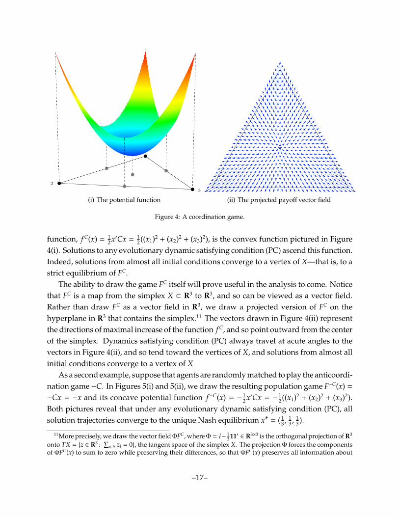
(i) The potential function (ii) The projected payoff vector field

Figure 4: A coordination game.

function, f C(x) = 12x′Cx = 1

2 ((x1)2 + (x2)2 + (x3)2), is the convex function pictured in Figure4(i). Solutions to any evolutionary dynamic satisfying condition (PC) ascend this function.Indeed, solutions from almost all initial conditions converge to a vertex of X—that is, to astrict equilibrium of FC.

The ability to draw the game FC itself will prove useful in the analysis to come. Noticethat FC is a map from the simplex X ⊂ R3 to R3, and so can be viewed as a vector field.Rather than draw FC as a vector field in R3, we draw a projected version of FC on thehyperplane in R3 that contains the simplex.11 The vectors drawn in Figure 4(ii) representthe directions of maximal increase of the function f C, and so point outward from the centerof the simplex. Dynamics satisfying condition (PC) always travel at acute angles to thevectors in Figure 4(ii), and so tend toward the vertices of X, and solutions from almost allinitial conditions converge to a vertex of X

As a second example, suppose that agents are randomly matched to play the anticoordi-nation game −C. In Figures 5(i) and 5(ii), we draw the resulting population game F−C(x) =

−Cx = −x and its concave potential function f −C(x) = −12x′Cx = − 1

2 ((x1)2 + (x2)2 + (x3)2).Both pictures reveal that under any evolutionary dynamic satisfying condition (PC), allsolution trajectories converge to the unique Nash equilibrium x∗ = (1

3 ,13 ,

13 ).

11More precisely, we draw the vector field ΦFC, where Φ = I− 13 11′ ∈ R3×3 is the orthogonal projection of R3

onto TX = {z ∈ R3 :∑

i∈S zi = 0}, the tangent space of the simplex X. The projection Φ forces the componentsof ΦFC(x) to sum to zero while preserving their differences, so that ΦFC(x) preserves all information about

–17–

(i) The potential function (ii) The projected payoff vector field

Figure 5: An anticoordination game.

4.2.2 The Hypnodisk Game

We now use the coordination game FC and the anticoordination game F−C to constructour replacement for bad RPS. While FC and F−C are potential games with linear payoffs,our new game will have neither of these properties.

The construction is easiest to describe in geometric terms. Begin with the coordinationgame FC(x) = Cx pictured in Figure 4(ii). Then draw two circles centered at state x∗ =

( 13 ,

13 ,

13 ) with radii 0 < r < R < 1

√6, as shown in Figure 6(i); the second inequality ensures

that both circles are contained in the simplex. Finally, twist the portion of the vector fieldlying outside of the inner circle in a clockwise direction, excluding larger and larger circlesas the twisting proceeds, so that the outer circle is reached when the total twist is 180◦.The resulting vector field is pictured in Figure 6(ii). It is described analytically by

H(x) = cos(θ(x))

x1 −

13

x2 −13

x3 −13

+

√3

3sin(θ(x))

x2 − x3

x3 − x1

x1 − x2

+13

111

,where θ(x) equals 0 when

∣∣∣x − x∗∣∣∣ ≤ r, equals π when

∣∣∣x − x∗∣∣∣ ≥ R, and varies linearly in

between. We call the game H the hypnodisk game.

incentives contained in payoff vector FC(x).

–18–

(i) Projected payoff vector field for the coordination game

(ii) Projected payoff vector field for the hypnodisk game

Figure 6: Construction of the hypnodisk game.

–19–

What does this construction accomplish? Inside the inner circle, H is identical to thecoordination game FC. Thus, solutions to dynamics satisfying (PC) starting at states in theinner circle besides x∗ must leave the inner circle. At states outside the outer circle, thedrawing of H is identical to the drawing of the anticoordination game F−C.12 Therefore,solutions to dynamics satisfying (PC) that begin outside the outer circle must enter theouter circle. Finally, at each state x in the annulus bounded by the two circles, H(x) is not acomponentwise constant vector. Therefore, states in the annulus are not Nash equilibria,and so are not rest points of dynamics satisfying (PC). We assemble these observations inthe following lemma.

Lemma 4.2. Suppose that V is an evolutionary dynamic that satisfies conditions (C) and (PC),and let H be the hypnodisk game. Then every solution to VH other than the stationary solution atx∗ enters the annulus with radii r and R and never leaves.

In fact, since there are no rest points in the annulus, the Poincare-Bendixson Theoremimplies that every nonstationary solution to VH converges to a limit cycle.

4.2.3 The Twin

Now, let F be the four-strategy game obtained from H by adding a twin: Fi(x1, x2, x3, x4) =

Hi(x1, x2, x3 + x4) for i ∈ {1, 2, 3}, and F4(x) = F3(x). The set of Nash equilibria of F is the linesegment

NE ={x∗ ∈ X : x∗1 = x∗2 = x∗3 + x∗4 = 1

3

}.

Let

I ={x ∈ X : (x1 −

13 )2 + (x2 −

13 )2 + (x3 + x4 −

13 )2≤ r2

}and

O ={x ∈ X : (x1 −

13 )2 + (x2 −

13 )2 + (x3 + x4 −

13 )2≤ R2

}be concentric cylindrical regions in X surrounding NE, as pictured in Figure 7. By con-struction, we have that

F(x) = Cx =

1 0 0 00 1 0 00 0 1 10 0 1 1

x1

x2

x3

x4

.12At states x outside the outer circle, H(x) = −x + 2

3 1 , −x = F−C(x). But since ΦH(x) = −x + 13 1 = ΦF−C(x)

at these states, the pictures of H and F−C, and hence the incentives in the two games, are the same.

–20–

Figure 7: Regions O, I, and D = O − I.

at all x ∈ I. Therefore, solutions to dynamics satisfying (PC) starting in I −NE ascend thepotential function f C(x) = 1

2 ((x1)2 + (x2)2 + (x3 +x4)2) until leaving the set I. At states outsidethe set O, we have that F(x) = −Cx, so solutions starting in X −O ascend f −C(x) = − f C(x)until entering O. In summary:

Lemma 4.3. Suppose that V is an evolutionary dynamic that satisfies conditions (C) and (PC),and let F be the “hypnodisk with a twin” game. Then every solution to VF other than the stationarysolutions at states in NE enter region D = O − I and never leave.

4.2.4 The Feeble Twin

To prove Theorem 3.1, we argued in Lemma 3.3 that under any of the dynamicsaddressed by the theorem, nonstationary solution trajectories equalize the utilizationlevels of identical twin strategies. If we presently focus on dynamics that not only satisfyconditions (C), (PC), and (IN), but also treat different strategies symmetrically, we canargue that in the “hypnodisk with a twin” game F, all nonstationary solutions of VF

converge not only to region D, but also to the plane P = {x ∈ X : x3 = x4}. Continuingwith the argument from Section 3 then allows us to conclude that in Fd, the game obtainedfrom F by turning strategy 4 into a feeble twin (that is, by reducing the payoff to strategy

–21–

Figure 8: The best response correspondence of the hypnodisk game.

4 uniformly by d > 0), the fraction x4 playing the feeble twin exceeds 16 infinitely often.

Since we would like a result that imposes as little structure as possible on permissibleevolutionary dynamics, Theorem 4.1 avoids the assumption that different strategies aretreated symmetrically. Since this means that agents may well be biased against choosingthe dominated strategy, we can no longer prove that the fraction playing it will repeatedlyexceed 1

6 . But we can still prove that the dominated strategy survives. To accomplishthis, it is enough to show that in game F, most solutions of the dynamic VF convergeto a set on which x4 is bounded away from 0. If we can do this, then repeating thecontinuity argument that concluded the proof of Theorem 3.1 shows that in the game Fd,the dominated strategy 4 survives.

A complete proof that most solutions of VF converge to a set on which x4 boundedaway from 0 is presented in Appendix C. We summarize the argument here. To begin, itcan be shown that all solutions to VF starting outside a small neighborhood of the segmentof Nash equilibria NE converge to an attractor A , a compact set that is contained in regionD and that is an invariant set of the dynamic VF.

Now suppose by way of contradiction that the attractor A intersects Z = {x ∈ X : x4 = 0},the face of X on which Twin is unused. The Lipschitz continuity of the dynamic VF

implies that backward solutions starting in Z cannot enter X − Z. Since A is forwardand backward invariant under VF, the fact that A intersects Z implies the existence of aclosed orbit γ ⊂ A ∩ Z that circumnavigates the disk I ∩ Z. Examining the best response

–22–

correspondence of the hypnodisk game (Figure 8), we find that such an orbit γ must passthrough a region in which strategy 3 is a best response. But since the twin strategy 4 isalso a best response in this region, innovation (IN) tells us that solutions passing throughthis region must reenter the interior of X, contradicting that the attractor A intersects theface Z.

5. Discussion

5.1 Constructing Games in which Dominated Strategies Survive

If an evolutionary dynamic satisfies monotonicity condition (PC), all of its rest pointsare Nash equilibria. It follows that dominated strategies can only survive on solutiontrajectories that do not converge to rest points. To construct games in which dominatedstrategies can survive, one should first look for games in which convergence rarely occurs.

The hypnodisk game, the starting point for the proof of the main theorem, is a pop-ulation game with nonlinear payoff functions. Such games were uncommon in the earlyliterature on evolution in games, which focused on random matching settings. But pop-ulation games with nonlinear payoffs are more common now, in part because of theirappearance in applications. For example, the standard model of driver behavior in ahighway network is a congestion game with nonlinear payoff functions, as delays on eachnetwork link are increasing, convex functions of the number of drivers using the link.13

For this reason, we do not view the use of a game with nonlinear payoffs as a shortcomingof our analysis. But despite this, it seems worth asking whether our results could beproved within the linear, random matching framework.

In Section 3, where we considered dynamics with prespecified functional forms, wewere able to prove survival results within the linear setting. More generally, if we fixan evolutionary dynamic before seeking a population game, finding a linear game thatexhibits cycling seems a feasible task. Still, a virtue of our analysis in Section 4 is that itavoids this case-by-case analysis: the hypnodisk game generates cycling under all of therelevant dynamics simultaneously, enabling us to prove survival of dominated strategiesunder all of these dynamics at once.

Could we have done the same using linear payoffs? Consider the following game due

13Congestion games with a continuum of agents are studied by Beckmann et al. (1956) and Sandholm(2001). For finite player congestion games, see Rosenthal (1973) and Monderer and Shapley (1996).

–23–

to Hofbauer and Swinkels (1996) (see also (Hofbauer and Sigmund, 1998, Sec 8.6)):

Fε(x) = Aεx =

0 0 −1 ε

ε 0 0 −1−1 ε 0 00 −1 ε 0

x.

When ε = 0, the game F0 is a potential game with potential function f (x) = −(x1x3 + x2x4).It has two components of Nash equilibria: one is a singleton containing the completelymixed equilibrium x∗ = (1

4 ,14 ,

14 ,

14 ); the other is the closed curve γ containing edges e1e2 ,

e2e3, e3e4, and e4e1. The former component is a saddle point of f , and so is unstable underdynamics that satisfy (PC); the latter component is the maximizer set of f , and so attractsmost solutions of these dynamics.

If ε is positive but sufficiently small, Theorem A.1 implies that most solutions ofdynamics satisfying (PC) lead to an attractor near γ. But once ε is positive, the uniqueNash equilibrium of Fε is the mixed equilibrium x∗. Therefore, the attractor near γ is farfrom any Nash equilibrium.

If we now introduce a feeble twin, we expect that this dominated strategy wouldsurvive in the resulting five-strategy game. But in this case, evolutionary dynamics runon a four-dimensional state space. Proving survival results when the dimension of thestate space exceeds three is very difficult, even if we fix the dynamic under considerationin advance. This points to another advantage of the hypnodisk game: it allows us to workwith dynamics on a three-dimensional state space, where the analysis is still tractable.

5.2 How Dominated Can Surviving Strategies Be?

Since the dynamics we consider are nonlinear, our proofs of survival of dominatedstrategies are topological in nature, and so do not quantify the level of domination that isconsistent with a dominated strategy maintaining a significant presence in the population.We can provide a sense of this magnitude by way of numerical analysis.

Our analysis considers the behavior of the BNN and Smith dynamics in the followingversion of “bad RPS with a feeble twin”:

(7) Fd(x) = Adx =

0 −2 1 11 0 −2 −2−2 1 0 0−2 − d 1 − d −d −d

x1

x2

x3

x4

.

–24–

Figure 9(i) presents the maximum, time-average, and minimum weight on the dominatedstrategy in the limit cycle of the BNN dynamic, with these weights being presented asfunctions of the domination level d. The figure shows that until the dominated strategyTwin is eliminated, its presence declines at roughly linear rate in d. Twin is playedrecurrently by at least 10% of the population when d ≤ .14, by at least 5% of the populationwhen d ≤ .19, and by at least 1% of the population when d ≤ .22.

Figure 9(ii) shows that under the Smith dynamic, the decay in the use of the dominatedstrategy is much more gradual. In this case, Twin is recurrently played by at least 10% ofthe population when d ≤ .31, by at least 5% of the population when d ≤ .47, and by at least1% of the population when d ≤ .66. These values of d are surprisingly large relative tothe base payoff values of 0, −2, and 1: even strategies that are dominated by a significantmargin can be played in perpetuity under common evolutionary dynamics.

The reason for the difference between the two dynamics is easy to explain. As we sawin Section 3, the BNN dynamic describes the behavior of agents who compare a candidatestrategy’s payoff with the average payoff in the population. For its part, the Smith dynamicis based on comparisons between the candidate strategy’s payoff and an agent’s currentpayoff. The latter specification makes it relatively easy for agents obtaining a low payoff

from Paper or Rock to switch to the dominated strategy Twin.

5.3 Exact and Hybrid Imitative Dynamics

An important class of dynamics excluded by our results are imitative dynamics, a classthat includes the replicator dynamic as its best-known example. In general, imitativedynamics are derived from revision protocols of the form

ρi j(π, x) = x jri j(π, x).

The x j term reflects the fact that when an agent receives a revision opportunity, he selects anopponent at random, and then decides whether or not to imitate this opponent’s strategy.Substituting ρ into equation (1), we see that imitative dynamics take the simple form

xi = xi

∑j∈S

x j

(r ji(F(x), x) − ri j(F(x), x)

)(8)

≡ xi pi(F(x), x).

In other words, each strategy’s absolute growth rate xi is proportional to its level ofutilization xi.

–25–

Ê

Ê

Ê

Ê

Ê

Ê

Ê

Ê

Ê

Ê

Ê

Ê

Ê

Ê

Ê

Ê

Ê

Ê

Ê

Ê

Ê

Ê

Ê

ÊÊÊÊÊÊÊÊÊÊÊÊÊÊÊÊÊÊÊÊÊÊÊÊÊÊÊÊ

‡‡‡‡‡‡‡‡‡‡‡‡‡‡‡‡‡‡‡‡‡‡‡‡‡‡‡‡‡‡‡‡‡‡‡‡‡‡‡‡‡‡‡‡‡‡‡‡‡‡‡

ÏÏÏÏÏÏÏÏÏÏÏÏÏÏÏÏÏÏÏÏÏÏÏÏÏÏÏÏÏÏÏÏÏÏÏÏÏÏÏÏÏÏÏÏÏÏÏÏÏÏÏ

0.0 0.1 0.2 0.3 0.4 0.5

0.05

0.10

0.15

0.20

0.25

(i) BNN

Ê

ÊÊÊÊÊÊÊÊÊÊÊÊÊÊÊÊÊÊÊÊÊÊÊÊÊÊÊÊÊÊÊÊÊÊÊÊÊÊÊÊÊÊÊÊÊÊÊÊÊÊÊÊÊÊÊÊÊÊÊÊÊÊÊÊÊÊÊÊÊÊÊÊÊÊÊÊÊÊÊÊÊÊÊÊÊÊÊÊÊÊÊÊÊÊÊÊÊÊÊÊ

‡‡‡‡‡‡‡‡‡‡‡‡‡‡‡‡‡‡‡‡‡‡‡‡‡‡‡‡‡‡‡‡‡‡‡‡‡‡‡‡‡‡‡‡‡‡‡‡‡‡‡‡‡‡‡‡‡‡‡‡‡‡‡‡‡‡‡‡‡‡‡‡‡‡‡‡‡‡‡‡‡‡‡‡‡‡‡‡‡‡‡‡‡‡‡‡‡‡‡‡‡

ÏÏÏÏÏÏÏÏÏÏÏÏÏÏÏÏÏÏÏÏÏÏÏÏÏÏÏÏÏÏÏÏÏÏÏÏÏÏÏÏÏÏÏÏÏÏÏÏÏÏÏÏÏÏÏÏÏÏÏÏÏÏÏÏÏÏÏÏÏÏÏÏÏÏÏÏÏÏÏÏÏÏÏÏÏÏÏÏÏÏÏÏÏÏÏÏÏÏÏÏÏ

0.2 0.4 0.6 0.8 1.0

0.05

0.10

0.15

0.20

0.25

(ii) Smith

Figure 9: The maximum, time-average, and minimum weight on the dominated strategy in thelimit cycles of the BNN and Smith dynamics. These weights are presented as functions of the

domination level d in game (7).

–26–

To see the consequences of this for dominated strategies, use equation (8) and thequotient rule to obtain

(9)ddt

(xi

x j

)=

xi

x j

(pi(F(x), x) − p j(F(x), x)

).

Now suppose that percentage growth rates are monotone, in the sense that

pi(π, x) ≥ p j(π, x) if and only if πi ≥ π j,

Then if strategy i strictly dominates strategy j, the right hand side of equation (9) is positiveat all x ∈ int(X). We can therefore conclude that the dominated strategy j vanishes alongevery interior solution trajectory of (8). This is Samuelson and Zhang’s (1992) eliminationresult.14

Equation (9) can be used to explain why elimination results for imitative dynamics arefragile. Suppose now that strategies i and j always earn the same payoffs. In this case,the right hand side of equation (9) is identically zero on int(X), implying that the ratio xi

x j

is constant along every interior solution trajectory. For instance, in Figure 10(i), a phasediagram of the replicator dynamic in “standard RPS with a twin”, we see that the planeson which the ratio xS

xTis constant are invariant sets. If we make the twin feeble by lowering

its payoff uniformly by d, we obtain the dynamics pictured in Figure 10(ii): now the ratioxSxT

increases monotonically, and the dominated strategy is eliminated.The existence of a continuum of invariant hyperplanes in games with identical twins

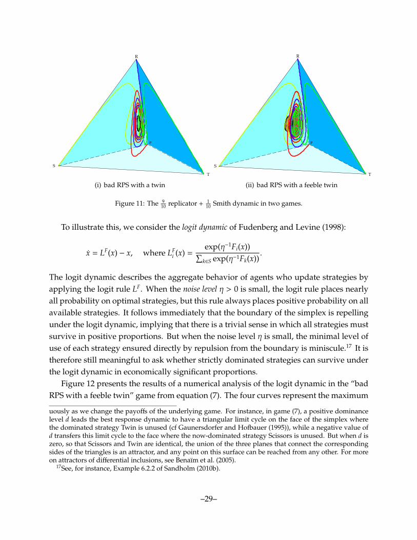
is crucial to this argument. At the same time, dynamics with a continuum of invarianthyperplanes are structurally unstable. If we fix the game but slightly alter the agents’revision protocol, these invariant sets can collapse, overturning the elimination result.

As an example, suppose that instead of always following an imitative protocol, agentsoccasionally use a protocol that allows switches to unused strategies. This situationis illustrated in Figure 11(i), which contains the phase diagram for a “bad RPS with atwin” game under a convex combination of the replicator and Smith dynamics.15 WhileFigure 10(i) displayed a continuum of invariant hyperplanes, Figure 11(i) shows almost

14Sandholm et al. (2008) establish close links between the replicator dynamic and the projection dynamicof Nagurney and Zhang (1997). They show that on the interior of the simplex, these two dynamics sharea property called “inflow-outflow symmetry”, which ensures that dominated strategies lose ground to thestrategies that dominate them. But the projection dynamic is discontinuous at the boundary of the simplex,and its behavior on the boundary can allow dominated strategies to survive.

15In particular, we consider the bad RPS game with payoffs 0, − 1110 , and 1, and the combined dynamic that

puts weight 910 on the replicator dynamic and weight 1

10 on the Smith dynamic. This dynamic is generated bythe corresponding convex combination of the underlying revision protocols: ρi j = 9

10 x j[F j−Fi]+ + 110 [F j−Fi]+.

–27–

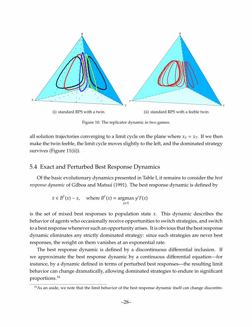
R

P

S

T

(i) standard RPS with a twin

R

P

S

T

(ii) standard RPS with a feeble twin

Figure 10: The replicator dynamic in two games.

all solution trajectories converging to a limit cycle on the plane where xS = xT. If we thenmake the twin feeble, the limit cycle moves slightly to the left, and the dominated strategysurvives (Figure 11(ii)).

5.4 Exact and Perturbed Best Response Dynamics

Of the basic evolutionary dynamics presented in Table I, it remains to consider the bestresponse dynamic of Gilboa and Matsui (1991). The best response dynamic is defined by

x ∈ BF(x) − x, where BF(x) = argmaxy∈X

y′F(x)

is the set of mixed best responses to population state x. This dynamic describes thebehavior of agents who occasionally receive opportunities to switch strategies, and switchto a best response whenever such an opportunity arises. It is obvious that the best responsedynamic eliminates any strictly dominated strategy: since such strategies are never bestresponses, the weight on them vanishes at an exponential rate.

The best response dynamic is defined by a discontinuous differential inclusion. Ifwe approximate the best response dynamic by a continuous differential equation—forinstance, by a dynamic defined in terms of perturbed best responses—the resulting limitbehavior can change dramatically, allowing dominated strategies to endure in significantproportions.16

16As an aside, we note that the limit behavior of the best response dynamic itself can change discontin-

–28–

R

P

S

T

(i) bad RPS with a twin

R

P

S

T

(ii) bad RPS with a feeble twin

Figure 11: The 910 replicator + 1

10 Smith dynamic in two games.

To illustrate this, we consider the logit dynamic of Fudenberg and Levine (1998):

x = LF(x) − x, where LFi (x) =

exp(η−1Fi(x))∑k∈S exp(η−1Fk(x))

.

The logit dynamic describes the aggregate behavior of agents who update strategies byapplying the logit rule LF. When the noise level η > 0 is small, the logit rule places nearlyall probability on optimal strategies, but this rule always places positive probability on allavailable strategies. It follows immediately that the boundary of the simplex is repellingunder the logit dynamic, implying that there is a trivial sense in which all strategies mustsurvive in positive proportions. But when the noise level η is small, the minimal level ofuse of each strategy ensured directly by repulsion from the boundary is miniscule.17 It istherefore still meaningful to ask whether strictly dominated strategies can survive underthe logit dynamic in economically significant proportions.

Figure 12 presents the results of a numerical analysis of the logit dynamic in the “badRPS with a feeble twin” game from equation (7). The four curves represent the maximum

uously as we change the payoffs of the underlying game. For instance, in game (7), a positive dominancelevel d leads the best response dynamic to have a triangular limit cycle on the face of the simplex wherethe dominated strategy Twin is unused (cf Gaunersdorfer and Hofbauer (1995)), while a negative value ofd transfers this limit cycle to the face where the now-dominated strategy Scissors is unused. But when d iszero, so that Scissors and Twin are identical, the union of the three planes that connect the correspondingsides of the triangles is an attractor, and any point on this surface can be reached from any other. For moreon attractors of differential inclusions, see Benaım et al. (2005).

17See, for instance, Example 6.2.2 of Sandholm (2010b).

–29–

Ê

Ê

Ê

Ê

ÊÊÊÊÊÊÊÊÊÊÊÊÊÊÊÊÊÊÊÊÊÊÊÊÊÊÊÊÊÊÊÊÊÊÊÊÊÊÊÊÊÊÊÊÊÊÊÊÊÊÊÊÊÊÊÊÊÊÊÊÊÊÊÊÊÊÊÊÊÊÊÊÊÊÊÊÊÊÊÊÊÊÊÊÊÊÊÊÊÊÊÊÊÊÊÊÊ

Ê

Ê

Ê

Ê

Ê

Ê

Ê

Ê

Ê

Ê

Ê

Ê

Ê

Ê

Ê

ÊÊÊÊÊÊÊÊÊÊÊÊÊÊÊÊÊÊÊÊÊÊÊÊÊÊÊÊÊÊÊÊÊÊÊÊÊÊÊÊÊÊÊÊÊÊÊÊÊÊÊÊÊÊÊÊ

‡

‡

‡

‡

‡

‡

‡

‡

‡

‡

‡

‡

‡‡‡‡‡‡‡‡‡‡‡‡‡‡‡‡‡‡‡‡‡‡‡‡‡‡‡‡‡‡‡‡‡‡‡‡‡‡‡‡‡‡‡‡‡‡‡‡‡‡‡‡‡‡‡‡‡‡‡‡‡‡‡‡‡‡‡‡‡‡‡‡‡‡‡‡‡‡‡‡‡‡‡‡‡‡‡‡‡

‡‡‡‡‡‡‡‡‡‡‡‡‡‡‡‡‡‡‡‡‡‡‡‡‡‡‡‡‡‡‡‡‡‡‡‡‡‡‡‡‡‡‡‡‡‡‡‡‡‡‡‡‡‡‡‡‡‡‡‡‡‡‡‡‡‡‡‡‡‡‡‡‡‡‡‡‡‡‡‡‡‡‡‡‡‡‡‡‡‡‡‡‡‡‡‡‡‡‡‡‡‡‡‡‡‡‡‡‡‡‡‡‡‡‡‡‡‡‡‡‡‡‡‡‡‡‡‡‡‡‡‡‡‡‡‡‡‡‡‡‡‡‡‡‡‡‡‡‡‡‡‡‡‡‡‡‡‡‡‡‡‡‡‡‡‡‡‡‡‡‡‡‡‡‡‡‡‡‡‡‡‡‡‡‡‡‡‡‡‡‡‡‡‡‡‡‡‡‡‡‡‡‡‡‡‡‡‡‡‡‡‡‡‡‡‡‡‡‡‡‡‡‡‡‡‡

Ï

Ï

Ï

Ï

Ï

Ï

Ï

Ï

ÏÏÏÏÏÏÏÏÏÏÏÏÏÏÏÏÏÏÏÏÏÏÏÏÏÏÏÏÏÏÏÏÏÏÏÏÏÏÏÏÏÏÏÏÏÏÏÏÏÏÏÏÏÏÏÏÏÏÏÏÏÏÏÏÏÏÏÏÏÏÏÏÏÏÏÏÏÏÏÏÏÏÏÏÏÏÏÏÏÏÏÏÏ

ÏÏÏÏÏÏÏÏÏÏÏÏÏÏÏÏÏÏÏÏÏÏÏÏÏÏÏÏÏÏÏÏÏÏÏÏÏÏÏÏÏÏÏÏÏÏÏÏÏÏÏÏÏÏÏÏÏÏÏÏÏÏÏÏÏÏÏÏÏÏÏÏÏÏÏÏÏÏÏÏÏÏÏÏÏÏÏÏÏÏÏÏÏÏÏÏÏÏÏÏÏÏÏÏÏÏÏÏÏÏÏÏÏÏÏÏÏÏÏÏÏÏÏÏÏÏÏÏÏÏÏÏÏÏÏÏÏÏÏÏÏÏÏÏÏÏÏÏÏÏÏÏÏÏÏÏÏÏÏÏÏÏÏÏÏÏÏÏÏÏÏÏÏÏÏÏÏÏÏÏÏÏÏÏÏÏÏÏÏÏÏÏÏÏÏÏÏÏÏÏÏÏÏÏÏÏÏÏÏÏÏÏÏÏÏÏÏÏÏÏÏÏÏÏÏÏÏÏÏÏÏÏÏÏÏÏÏÏÏÏÏÏÏÏÏÏÏÏÏÏÏÏÏÏÏÏÏÏÏÏÏÏÏÏÏÏÏÏÏÏÏÏÏÏÏÏÏÏÏÏÏÏÏÏÏÏÏÏÏÏÏÏÏÏÏÏÏÏÏÏÏÏÏÏÏÏÏÏÏÏÏÏÏÏÏÏÏÏÏÏÏÏÏÏÏÏÏÏÏÏÏÏÏÏÏÏÏÏÏÏÏÏÏÏÏÏÏÏÏÏÏÏÏÏÏÏÏÏÏÏÏÏÏÏÏÏÏÏÏÏÏÏÏÏÏÏÏÏÏÏÏÏÏÏÏÏÏÏÏÏÏÏÏÏÏÏÏÏÏÏÏ

ÚÚÚÚÚÚÚÚÚÚÚÚÚÚÚÚÚÚÚÚÚÚÚÚÚÚÚÚÚÚÚÚÚÚÚÚÚÚÚÚÚÚÚÚÚÚÚÚÚÚÚÚÚÚÚÚÚÚÚÚÚÚÚÚÚÚÚÚÚÚÚÚÚÚÚÚÚÚÚÚÚÚÚÚÚÚÚÚÚÚÚÚÚÚÚÚÚÚÚÚÚ

0.0 0.2 0.4 0.6 0.8 1.0

0.05

0.10

0.15

0.20

0.25

0.30

h =.01h =.05

h =.10h =.20

Figure 12: The maximum weight on the dominated strategy in limit cycles of the logit(η) dynamic,η = .01, .05, .10, and .20, in game (7). Weights are presented as functions of the domination level d.

weight on the dominated strategy Twin in the stable limit cycle of the logit(η) dynamicfor noise levels η = .01, .05, .10, and .20.18 In each case, the weight on Twin is presented asa function of the domination level d in game (7).

When both the noise level η and the domination level d are very close to 0, the weighton the dominated strategy Twin recurrently approaches values of nearly 2

7 .19 For smallfixed values of η, the maximum weight on the dominated strategy falls rapidly as thedomination d level increases.

Higher values of η introduce more randomness into agents’ choices, creating a forcepushing the population state toward the center of the simplex. This inward force reducesthe maximal weight on the dominated strategy at low values of d, but allows the dominatedstrategy to maintain a significant presence at considerably higher values of d.

18To interpret the analysis, note that a noise level of η corresponds to the introduction of i.i.d. extreme-value distributed payoff disturbances with standard deviation πη/

√6 ≈ 1.28 η; see Anderson et al. (1992) or

Hofbauer and Sandholm (2002).19To see why, note that under the best response dynamic for bad RPS, the maximum weight on Scissors in

the limit cycle is 47 (see Gaunersdorfer and Hofbauer (1995)). If we move from the best response dynamic to a

low-noise logit dynamic, and introduce a slightly dominated strategy Twin, a total weight of approximately47 is split nearly evenly between Scissors and Twin.

–30–

5.5 On the Necessity of the Sufficient Conditions for Survival

Our main result shows that dynamics satisfying conditions (C), (PC), (NS) and (IN)fail to eliminate strictly dominated strategies in some games. While we believe that theseconditions are uncontroversial, it is still natural to ask whether they are obligatory to reachthe conclusions established here.

Our continuity condition, (C), seems unavoidable. This condition excludes best re-sponse dynamics, which satisfy the three remaining conditions and eliminate strictlydominated strategies in all games. Still, continuity is a natural restriction to impose ondynamics that aim to describe the behavior of myopic, imperfectly informed agents. Theresults in this paper can be viewed as a demonstration of one counterintuitive consequenceof this realistic requirement.

Our analysis in Section 4 uses innovation (IN) to establish that in the hypnodisk gamewith an exact twin, the mass placed on the twin strategy at states in the attractor A isbounded away from zero. It seems to us that in the presence of the other three conditions,a fourth condition significantly weaker than or of a different nature than condition (IN)might suffice for establishing survival results.

Positive correlation (PC) and Nash stationarity (NS) link the directions of motionunder an evolutionary dynamic and the identity of its stationary states to the payoffsin the game at hand. As such, they help us specify what we mean by an evolutionarydynamic. It is nevertheless worth asking whether conditions (NS) and (PC) are necessaryfor proving survival results. Suppose first that one follows the “uniform” approach fromSection 4, seeking a single game that generates nonconvergence and survival in the classof dynamics under consideration. Clearly, achieving this aim requires one to constrainthe class of dynamics by means of some general restrictions on the allowable directions ofmotion from each population state. We employ condition (PC) because it is the weakestcondition connecting payoffs to the direction of motion that appears in the literature, andwe employ condition (NS) because it restricts the set of stationary states in an economicallysensible away. Other conditions could be used instead to ensure the existence of a “badly-behaved” game; by combining these conditions with (C) and (IN), one could again obtainsurvival results.

Alternatively, one could consider a “non-uniform” approach, constructing a possiblydistinct game generating nonconvergence and survival for each dynamic under consid-eration. Given the attendant freedom to tailor the game to the dynamic at hand, it seemspossible that continuity (C) and Nash stationarity (NS) on their own might be enough toestablish a survival result. Proving such a result would require one to define a method ofassigning each evolutionary dynamic (i.e., each map from games to differential equations)

–31–

a “badly-behaved” game with a pair of twin strategies, and then to show that in eachcase, the resulting differential equation admits an interior attractor with a large basin ofattraction. Whether this approach can be brought to fruition is a challenging question forfuture research.

6. Conclusion

Traditional game-theoretic analyses rule out strictly dominated strategies, as playingsuch strategies is inconsistent with decision-theoretic rationality. This paper argues that insettings where evolutionary game models are appropriate, the justification for eliminatingdominated strategies is far less secure. When evolutionary dynamics converge, their limitsare equilibria of the underlying game, and so exclude strictly dominated strategies. Butguarantees of convergence are available only for a few classes of games. When dynamicsfail to converge, the payoffs of the available strategies remain in flux. If agents are not exactoptimizers, but instead choose among strategies whose current payoffs are reasonablyhigh, dominated strategies may be played by significant numbers of agents in perpetuity.

Appendix

A. Continuation of Attractors

Let X be a compact metric space and let φ be a semi-flow on X; thus, φ : [0,∞)×X→ Xis a continuous map satisfying φ0(x) = x and φt(φs(x)) = φt+s(x) for all s, t ≥ 0 and x ∈ X.A set A ⊂ X is an attractor of φ if there is a neighborhood U of A such that ω(U) = A (seeConley (1978)). Here the ω-limit set of U is defined as ω(U) =

⋂t>0 cl(φ[t,∞)(U)), where for

T ⊂ R we let φT(U) =⋃

t∈T φt(U) . An attractor is compact and invariant (φt(A) = A for all

t). Observe that an attractor can strictly contain another attractor.The basin of the attractor is defined as B(A) = {x : ω(x) ⊆ A}. For each open set U

with A ⊂ U ⊂ cl(U) ⊂ B(A) we have ω(cl(U)) = A, see Section II.5.1.A of Conley (1978).Furthermore, if φt(cl(U)) ⊂ U holds for some t > 0 and for some open set U (which is thencalled a trapping region), then ω(U) is an attractor, see Section II.5.1.C of Conley (1978).

For a flow (φt, t ∈ R), the complement of the basin B(A) of the attractor A is called thedual repellor of A. For all x ∈ B(A) − A, φt(x) approaches this dual repellor as t→ −∞.

Consider now a one-parameter family of differential equations x = Vε(x) in Rn (withunique solutions x(t) = Φt

ε(x(0)) such that (ε, x) 7→ Vε(x) is continuous. Then (ε, t, x) 7→Φtε(x) is continuous as well. Suppose that X ⊂ Rn is compact and forward invariant under

–32–

the semi-flows Φε. For ε = 0 we omit the subscript in Φt.The following continuation theorem for attractors is part of the folklore of dynamical

systems; compare, e.g., Proposition 8.1 of Smale (1967).

Theorem A.1. Let A be an attractor for Φ with basin B(A). Then for each small enough ε > 0 thereexists an attractor Aε of Φε with basin B(Aε), such that the map ε 7→ Aε is upper hemicontinuousand the map ε 7→ B(Aε) is lower hemicontinuous.

Upper hemicontinuity cannot be replaced by continuity in this result. Consider thefamily of differential equations x = (ε + x2)(1 − x) on the real line. The semi-flow Φ

corresponding to ε = 0 admits A = [0, 1] as an attractor, but when ε > 0 the uniqueattractor of Φε is Aε = {1}. This example shows that perturbations can cause attractors toimplode; the theorem shows that perturbations cannot cause attractors to explode.

Theorem A.1 is a direct consequence of the following lemma, which is sufficient toprove the results in Sections 3 and 4.

Lemma A.2. Let A be an attractor for Φ with basin B(A), and let U1 and U2 be open sets satisfyingA ⊂ U1 ⊆ U2 ⊆ cl(U2) ⊆ B(A). Then for each small enough ε > 0 there exists an attractor Aε ofΦε with basin B(Aε), such that Aε ⊂ U1 and U2 ⊂ B(Aε).

In this lemma, one can always set U1 = {x : dist(x,A) < δ} and U2 = {x ∈ B(A) : dist(x,X −B(A)) > δ} for some small enough δ > 0.

Proof of Lemma A.2. Since A is an attractor and ω(cl(U2)) = A, there is a T > 0 such thatΦt(cl(U2)) ⊂ U1 for t ≥ T. By the continuous dependence of the flow on the parameter εand the compactness of ΦT(cl(U2)), we have that ΦT

ε (cl(U2)) ⊂ U1 ⊆ U2 for all small enoughε. Thus, U2 is a trapping region for the semi-flow Φε, and Aε ≡ ω(U2) is an attractor forΦε. Moreover, Aε ⊂ U1 (since Aε = ΦT

ε (Aε) ⊆ ΦTε (cl(U2)) ⊂ U1) and U2 ⊂ B(Aε). �

B. Proofs Omitted from Section 3

B.1 The Proof of Lemma 3.2

Lemma 3.2 states that the set of Nash equilibria NE = {x∗ ∈ X : x∗ = ( 13 ,

13 , α,

13 − α)} in

the “bad RPST” game F(x) = Ax is a repellor under the dynamics defined in Theorem 3.1.These dynamics are generated by revision protocols of the forms

ρi j = φ(F j − F) and(2)

–33–

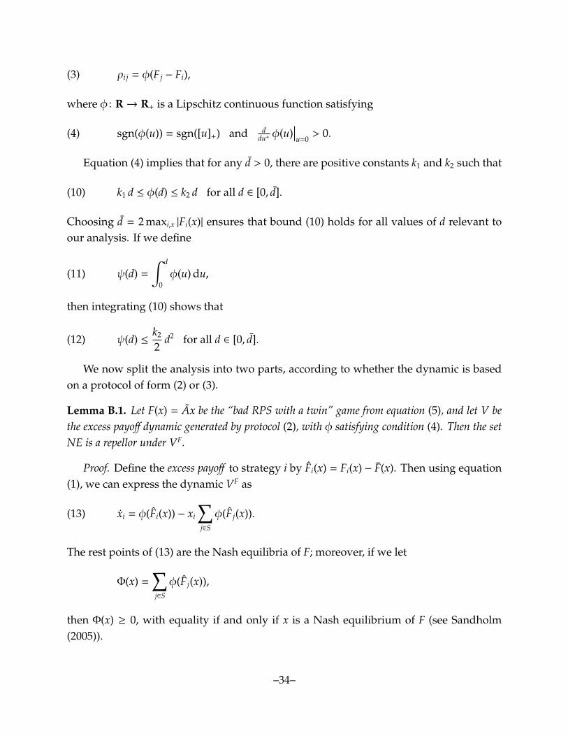
ρi j = φ(F j − Fi),(3)

where φ : R→ R+ is a Lipschitz continuous function satisfying

(4) sgn(φ(u)) = sgn([u]+) and ddu+ φ(u)

∣∣∣u=0

> 0.

Equation (4) implies that for any d > 0, there are positive constants k1 and k2 such that

(10) k1 d ≤ φ(d) ≤ k2 d for all d ∈ [0, d].

Choosing d = 2 maxi,x |Fi(x)| ensures that bound (10) holds for all values of d relevant toour analysis. If we define

(11) ψ(d) =

∫ d

0φ(u) du,

then integrating (10) shows that

(12) ψ(d) ≤k2

2d2 for all d ∈ [0, d].

We now split the analysis into two parts, according to whether the dynamic is basedon a protocol of form (2) or (3).

Lemma B.1. Let F(x) = Ax be the “bad RPS with a twin” game from equation (5), and let V bethe excess payoff dynamic generated by protocol (2), with φ satisfying condition (4). Then the setNE is a repellor under VF.

Proof. Define the excess payoff to strategy i by Fi(x) = Fi(x) − F(x). Then using equation(1), we can express the dynamic VF as

(13) xi = φ(Fi(x)) − xi

∑j∈S

φ(F j(x)).

The rest points of (13) are the Nash equilibria of F; moreover, if we let

Φ(x) =∑j∈S

φ(F j(x)),

then Φ(x) ≥ 0, with equality if and only if x is a Nash equilibrium of F (see Sandholm(2005)).

–34–

Consider the Lyapunov function

U(x) =∑i∈S

ψ(Fi(x)),

where ψ is defined in equation (11). Hofbauer (2000) and Hofbauer and Sandholm (2009)show that U(x) ≥ 0, with equality holding if and only if x is a Nash equilibrium of F. Theproof of this theorem shows that the time derivative of U under the dynamic (13) can beexpressed as

(14) U(x) = x′Ax −Φ(x) F(x)′x.

To prove our lemma, we need to show that U(x) > 0 whenever x < NE and dist(x,NE) issufficiently small.

Let TX = {z ∈ R4 : z′1 = 0}, the tangent space of the simplex X, so that x ∈ TX, andsuppose that z ∈ TX. Then letting (ζ1, ζ2, ζ3) = (z1, z2, z3 + z4), we have that

z′Az = (a − b) (z1z2 + z2(z3 + z4) + (z3 + z4)z1)(15)

= (a − b) (ζ1ζ2 + ζ2ζ3 + ζ3ζ1)

=b − a

2

3∑

i=1

ζi

2

− 2∑

1≤i< j≤3

ζiζ j

=

b − a2

3∑i=1

ζ2i .

=b − a

2

((z1)2 + (z2)2 + (z3 + z4)2

).

Now if x < NE, we can write (13) as

(16) x = Φ(x) (σ(x) − x)

where σ(x) ∈ X is given by σi(x) = φ(Fi(x))/Φ(x). Since x < NE, some strategy i has a belowaverage payoff (Fi(x) < F(x)), implying that σi(x) = 0, and hence that σ(x) ∈ bd(X). In fact,since strategies 3 and 4 always earn the same payoff, we have that σ3(x) = 0 if and only ifσ4(x) = 0.

If we now write y = (x1, x2, x3 + x4) and τ(x) = (σ1(x), σ2(x), σ3(x) + σ4(x)), equation (16)becomes

y = Φ(x)(τ(x) − y).

–35–

The arguments in the previous paragraph show that τ(x) is on the boundary of the simplexin R3. Therefore, if we fix a small ε > 0 and assume that dist(x,NE) < ε, then

∣∣∣y − ( 13 ,

13 ,

13 )∣∣∣ <

ε, giving us a uniform bound on the distance between τ(x) and y, and hence a uniformlower bound on

∣∣∣y∣∣∣:∣∣∣y∣∣∣ ≥ c Φ(x)

for some c > 0. By squaring and rewriting in terms of x, we obtain

(17) x21 + x2

2 + (x3 + x4)2≥ c2 Φ(x)2.

Thus, combining equations (15) and (17) shows that if dist(x,NE) < ε, then

(18) x′Ax ≥ b−a2 c2 Φ(x)2.

To bound the second term of equation (14), use equation (10) to show that

Φ(x) F(x)′x = Φ(x) (F(x) − F(x)1)′x(19)

= Φ(x) F(x)′x since 1′x = 0

= Φ(x)∑i∈S

Fi(x)(φ(Fi(x)) − xiΦ(x))

= Φ(x)∑i∈S

Fi(x)φ(Fi(x)) since F(x)′x = 0

≥ Φ(x) k1

∑i∈S

Fi(x)2

≥ Φ(x)k1

n

∑i∈S

Fi(x)

2

≥ Φ(x)k1

nk22

∑i∈S

φ(Fi(x))

2

=k1

nk22

Φ(x)3.

Combining inequalities (18) and (19) with equation (14), we find that for x close enoughto NE,

U(x) ≥b − a

2c2 Φ(x)2

−k1

nk22

Φ(x)3.

–36–

Since Φ(x) ≥ 0, with equality only when x ∈ NE, we conclude that U(x) > 0 wheneverx < NE is close enough to NE, and therefore that NE is a repellor under (13). �

Lemma B.2. Let F(x) = Ax be the “bad RPS with a twin” game from equation (5), and let V bethe pairwise comparison dynamic generated by protocol (3), with φ satisfying condition (4). Thenthe set NE is a repellor under VF.

Proof. Using equation (1), we express the dynamic VF as

(20) xi =∑j∈S

x jφ(Fi(x) − F j(x)) − xi

∑j∈S

φ(F j(x) − Fi(x)).

Sandholm (2010a) shows that the rest points of (20) are the Nash equilibria of F.Our analysis relies on the following Lyapunov function:

Ψ(x) =∑i∈S

∑j∈S

xiψ(F j(x) − Fi(x)),

whereψ is defined in equation (11). Hofbauer and Sandholm (2009) (also see Smith (1984))show that Ψ(x) ≥ 0, with equality holding if and only if x is a Nash equilibrium of F. Theproof of that theorem shows that the time derivative of Ψ under the dynamic (20) can beexpressed as

Ψ(x) = x′Ax +∑i∈S

∑j∈S

x j φ(Fi(x) − F j(x))∑k∈S

(ψ (Fk(x) − Fi(x)) − ψ(Fk(x) − F j(x))

)(21)

≡ T1(x) + T2(x).

Equation (15) tells us that T1(x) ≥ 0, with equality when x ∈ NE (i.e., when x = 0).Hofbauer and Sandholm (2009) show that T2(x) ≤ 0, with equality only when x ∈ NE. Toprove the lemma, we must show that T1(x) + T2(x) > 0 whenever x < NE and dist(x,NE)is sufficiently small.

To begin, observe that since F is linear, we have that

(22) [F j(x) − Fi(x)]+ ≤ c1 dist(x,NE).

for some c1 > 0. Equations (10), (12), and (22) immediately yield a cubic bound on T2:

(23) |T2(x)| ≤ c2 dist(x,NE)3

for some c2 > 0.

–37–

To obtain a lower bound on T1, first note that the linearity of F implies that

(24) maxi∈S

Fi(x) −minj∈S

F j(x) ≥ c3 dist(x,NE)

for some c3 > 0. If F1(x) ≥ F2(x) ≥ F3(x) = F4(x), then equations (10) and (24) imply that

x1 =

4∑j=2

x j φ(F1(x) − F j(x)) ≥ (x3 + x4)φ(F1(x) − F3(x)) ≥ (x3 + x4) c3 k1 dist(x,NE).

Similarly, if F1(x) ≤ F2(x) ≤ F3(x) = F4(x), then

|x1| = x1

4∑j=2

φ(F j(x) − F1(x)) ≥ x1φ(F3(x) − F1(x)) ≥ x1 c3 k1 dist(x,NE).

Obtaining bounds on |x1| and on |x2| for the remaining four cases in like fashion, wefind that for some c4 > 0 and some ε > 0, for any x with dist(x,NE) ≤ ε (and hence∣∣∣x1 −

13

∣∣∣ ≤ ε, ∣∣∣x2 −13

∣∣∣ ≤ ε, and∣∣∣(x3 + x4) − 1

3

∣∣∣ ≤ ε), we have that

(25) x21 + x2

2 + (x3 + x4)2≥ max(x2

1, x22) ≥ c4 dist(x,NE)2.

Thus, equations (15) and (25) together imply that for such x,

(26) T1 = x′Ax ≥ b−a2 c4 dist(x,NE)2.

Combining equations (21), (23), and (26), we find that

Ψ(x) ≥ b−a2 c4 dist(x,NE)2

− c2 dist(x,NE)3

whenever dist(x,NE) ≤ ε. We therefore conclude that Ψ(x) > 0 whenever x is sufficientlyclose to but not in NE, and so that NE is a repellor under (20). �

B.2 The Proof of Lemma 3.3

Let {xt}t≥0 be the solution to VF from initial condition ξ ∈ X−NE, and suppose withoutloss of generality that ξ3 ≥ ξ4. Then equation (6) implies that (x3 − x4)t is positive and isnonincreasing in t, while Lemma 3.2 reveals that there is a neighborhood U of of NE anda time T ≥ 0 such that {xt} ∈ X −U for all t ≥ T.

We split the remaining analysis into two cases. Suppose first that the revision protocol

–38–

ρ is of form (2), so that V is an excess payoff dynamic. In this case, equation (6) becomes

x3 − x4 = −(x3 − x4)∑j∈S

φ(F j(x) − F(x)) ≡ −(x3 − x4) Φ(x).

Sandholm (2005) shows that Φ(x) ≥ 0, with equality if and only if x is a Nash equilibrium ofF. Since U is an open neighborhood of NE, it follows that that m = minx∈X−U Φ(x) > 0. Thusddt (x3 − x4)t ≤ −m(x3 − x4)t for all t ≥ T, from which we conclude that limt→∞(x3 − x4)t = 0.

Now suppose that ρ is of form (3), so that V is a pairwise comparison dynamic. In thiscase, equation (6) becomes

(27) x3 − x4 = −(x3 − x4)∑j∈S

φ(F j(x) − F3(x)).

Since (x3 − x4)t is positive and is nonincreasing in t, it converges to some nonnegativelimit l. Thus, ω(ξ), the ω-limit set of trajectory {xt}, is contained in the plane Pl = {x ∈X : x3 − x4 = l}. Also, ω(ξ) is compact and invariant by definition (see, e.g., Robinson(1995)), and ω(ξ) is disjoint from NE by Lemma 3.2.

Now assume that l is positive. Then equation (27), combined with the fact that ω(ξ) isinvariant and a subset of Pl, implies that

∑j∈S φ(F j(x) − F3(x)) = 0 for all x ∈ ω(ξ). It then

follows from condition (4) (namely, from the fact that sgn(φ(u)) = sgn([u]+)) that strategy3 is optimal throughout ω(ξ); the identical twin strategy 4 must be so as well. But it iseasy to check that under any pairwise comparison dynamic VF for the “bad RPS with atwin” game F, optimal strategies have positive growth rates at any non-Nash state. Sinceω(ξ) is disjoint from NE, we conclude that VF

3 (x) + VF4 (x) > 0 whenever x ∈ ω(ξ).

At the same time, since ω(ξ) is compact, χ = argmaxx∈ω(ξ) x3 + x4 exists, and since ω(ξ)is also invariant, it must be that VF

3 (χ) + VF4 (χ) ≤ 0. This is a contradiction. We therefore

conclude that l = 0, and so that {xt} converges to the plane P0 = P. �

C. Proofs Details Omitted from Section 4.2.4

Our analysis relies on the notion of attractor-repellor pairs introduced by Conley (1978);see Robinson (1995) for a textbook treatment. Define the flow from the set U ⊆ X underthe dynamic VF by

φt(U) ={ξ ∈ X : there is a solution {xs} to x = VF(x) with x0 ∈ U and xt = ξ.

}

–39–

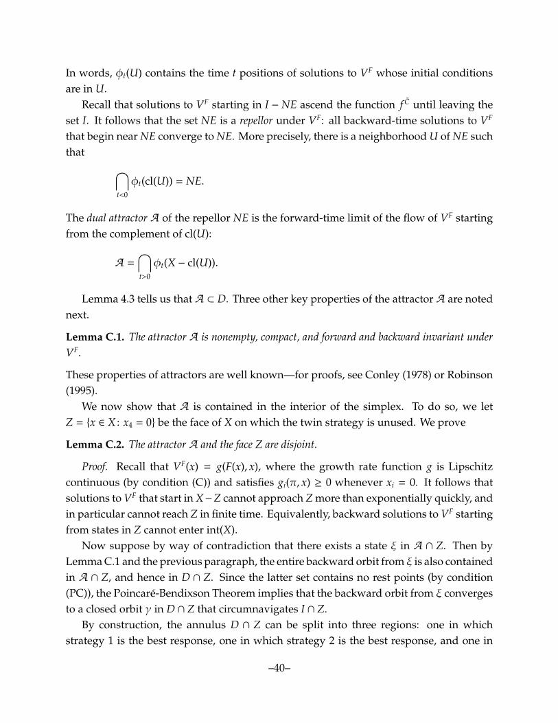
In words, φt(U) contains the time t positions of solutions to VF whose initial conditionsare in U.

Recall that solutions to VF starting in I − NE ascend the function f C until leaving theset I. It follows that the set NE is a repellor under VF: all backward-time solutions to VF

that begin near NE converge to NE. More precisely, there is a neighborhood U of NE suchthat ⋂

t<0

φt(cl(U)) = NE.

The dual attractor A of the repellor NE is the forward-time limit of the flow of VF startingfrom the complement of cl(U):

A =⋂t>0

φt(X − cl(U)).

Lemma 4.3 tells us that A ⊂ D. Three other key properties of the attractor A are notednext.

Lemma C.1. The attractor A is nonempty, compact, and forward and backward invariant underVF.

These properties of attractors are well known—for proofs, see Conley (1978) or Robinson(1995).

We now show that A is contained in the interior of the simplex. To do so, we letZ = {x ∈ X : x4 = 0} be the face of X on which the twin strategy is unused. We prove

Lemma C.2. The attractor A and the face Z are disjoint.

Proof. Recall that VF(x) = g(F(x), x), where the growth rate function g is Lipschitzcontinuous (by condition (C)) and satisfies gi(π, x) ≥ 0 whenever xi = 0. It follows thatsolutions to VF that start in X−Z cannot approach Z more than exponentially quickly, andin particular cannot reach Z in finite time. Equivalently, backward solutions to VF startingfrom states in Z cannot enter int(X).

Now suppose by way of contradiction that there exists a state ξ in A ∩ Z. Then byLemma C.1 and the previous paragraph, the entire backward orbit from ξ is also containedin A ∩ Z, and hence in D ∩ Z. Since the latter set contains no rest points (by condition(PC)), the Poincare-Bendixson Theorem implies that the backward orbit from ξ convergesto a closed orbit γ in D ∩ Z that circumnavigates I ∩ Z.

By construction, the annulus D ∩ Z can be split into three regions: one in whichstrategy 1 is the best response, one in which strategy 2 is the best response, and one in

–40–

which strategy 3 (and hence strategy 4) is a best response. Each of these regions is boundedby a simple closed curve that intersects the inner and outer boundaries of the annulus.Therefore, the closed orbit γ, on which strategy 4 is unused, passes through the region inwhich strategy 4 is optimal. This contradicts innovation (IN). �

References

Akin, E. (1980). Domination or equilibrium. Mathematical Biosciences, 50:239–250.

Anderson, S. P., de Palma, A., and Thisse, J.-F. (1992). Discrete Choice Theory of ProductDifferentiation. MIT Press, Cambridge.

Beckmann, M., McGuire, C. B., and Winsten, C. B. (1956). Studies in the Economics ofTransportation. Yale University Press, New Haven.

Benaım, M., Hofbauer, J., and Sorin, S. (2005). Stochastic approximations and differentialinclusions. SIAM Journal on Control and Optimization, 44:328–348.

Benaım, M. and Weibull, J. W. (2003). Deterministic approximation of stochastic evolutionin games. Econometrica, 71:873–903.

Berger, U. and Hofbauer, J. (2006). Irrational behavior in the Brown-von Neumann-Nashdynamics. Games and Economic Behavior, 56:1–6.

Binmore, K. and Samuelson, L. (1999). Evolutionary drift and equilibrium selection.Review of Economic Studies, 66:363–393.

Brown, G. W. and von Neumann, J. (1950). Solutions of games by differential equations. InKuhn, H. W. and Tucker, A. W., editors, Contributions to the Theory of Games I, volume 24of Annals of Mathematics Studies, pages 73–79. Princeton University Press, Princeton.

Conley, C. (1978). Isolated Invariant Sets and the Morse Index. American MathematicalSociety, Providence, RI.

Friedman, D. (1991). Evolutionary games in economics. Econometrica, 59:637–666.

Fudenberg, D. and Levine, D. K. (1998). Theory of Learning in Games. MIT Press, Cambridge.

Gaunersdorfer, A. and Hofbauer, J. (1995). Fictitious play, Shapley polygons, and thereplicator equation. Games and Economic Behavior, 11:279–303.

Gilboa, I. and Matsui, A. (1991). Social stability and equilibrium. Econometrica, 59:859–867.

Hart, S. and Mas-Colell, A. (2003). Uncoupled dynamics do not lead to Nash equilibrium.American Economic Review, 93:1830–1836.

–41–

Hofbauer, J. (2000). From Nash and Brown to Maynard Smith: Equilibria, dynamics, andESS. Selection, 1:81–88.

Hofbauer, J. and Sandholm, W. H. (2002). On the global convergence of stochastic fictitiousplay. Econometrica, 70:2265–2294.

Hofbauer, J. and Sandholm, W. H. (2009). Stable games and their dynamics. Journal ofEconomic Theory, 144:1665–1693.

Hofbauer, J. and Sigmund, K. (1998). Evolutionary Games and Population Dynamics. Cam-bridge University Press, Cambridge.

Hofbauer, J. and Swinkels, J. M. (1996). A universal Shapley example. Unpublishedmanuscript, University of Vienna and Northwestern University.

Hofbauer, J. and Weibull, J. W. (1996). Evolutionary selection against dominated strategies.Journal of Economic Theory, 71:558–573.

Jordan, J. S. (1993). Three problems in learning mixed-strategy Nash equilibria. Games andEconomic Behavior, 5:368–386.

Monderer, D. and Shapley, L. S. (1996). Potential games. Games and Economic Behavior,14:124–143.

Nachbar, J. H. (1990). ’Evolutionary’ selection dynamics in games: Convergence and limitproperties. International Journal of Game Theory, 19:59–89.

Nagurney, A. and Zhang, D. (1997). Projected dynamical systems in the formulation,stability analysis, and computation of fixed demand traffic network equilibria. Trans-portation Science, 31:147–158.

Robinson, C. (1995). Dynamical Systems: Stability, Symbolic Dynamics, and Chaos. CRCPress, Boca Raton, FL.

Rosenthal, R. W. (1973). A class of games possessing pure strategy Nash equilibria.International Journal of Game Theory, 2:65–67.

Samuelson, L. and Zhang, J. (1992). Evolutionary stability in asymmetric games. Journalof Economic Theory, 57:363–391.

Sandholm, W. H. (2001). Potential games with continuous player sets. Journal of EconomicTheory, 97:81–108.

Sandholm, W. H. (2003). Evolution and equilibrium under inexact information. Gamesand Economic Behavior, 44:343–378.

Sandholm, W. H. (2005). Excess payoff dynamics and other well-behaved evolutionarydynamics. Journal of Economic Theory, 124:149–170.

–42–

Sandholm, W. H. (2009a). Evolutionary game theory. In Meyers, R. A., editor, Encyclopediaof Complexity and Systems Science, pages 3176–3205. Springer, Heidelberg.

Sandholm, W. H. (2009b). Large population potential games. Journal of Economic Theory,144:1710–1725.

Sandholm, W. H. (2010a). Pairwise comparison dynamics and evolutionary foundationsfor Nash equilibrium. Games, 1:3–17.

Sandholm, W. H. (2010b). Population Games and Evolutionary Dynamics. MIT Press, Cam-bridge.

Sandholm, W. H. and Dokumacı, E. (2007). Dynamo: Phase diagrams for evolutionarydynamics. Software. http://www.ssc.wisc.edu/∼whs/dynamo.

Sandholm, W. H., Dokumacı, E., and Lahkar, R. (2008). The projection dynamic and thereplicator dynamic. Games and Economic Behavior, 64:666–683.

Shapley, L. S. (1964). Some topics in two person games. In Dresher, M., Shapley, L. S.,and Tucker, A. W., editors, Advances in Game Theory, volume 52 of Annals of MathematicsStudies, pages 1–28. Princeton University Press, Princeton.

Smale, S. (1967). Differentiable dynamical systems. Bulletin of the American MathematicalSociety, 73:747–817.

Smith, M. J. (1984). The stability of a dynamic model of traffic assignment—an applicationof a method of Lyapunov. Transportation Science, 18:245–252.

Sparrow, C., van Strien, S., and Harris, C. (2008). Fictitious play in 3 × 3 games: Thetransition between periodic and chaotic behaviour. Games and Economic Behavior, 63:259–291.

Swinkels, J. M. (1993). Adjustment dynamics and rational play in games. Games andEconomic Behavior, 5:455–484.

Taylor, P. D. and Jonker, L. (1978). Evolutionarily stable strategies and game dynamics.Mathematical Biosciences, 40:145–156.

Weibull, J. W. (1996). The mass action interpretation. Excerpt from ’The work of JohnNash in game theory: Nobel Seminar, December 8, 1994’. Journal of Economic Theory,69:165–171.

–43–