Surface Water Treatment Rule - clark.wa.gov · Guidance Manual. Surface Water Treatment Rule ....

Guidance Manual

Surface Water Treatment Rule

September 1995

We created this electronic copy from the original 1995 version. Although it looks different, the content is the same.

DOH 331-085

Guidance Manual

Surface Water Treatment Rule September 1995

For more information or additional copies of this publication contact:

Office of Drinking Water Department of Health PO Box 47828 Olympia, WA 98504-7828 (360) 236-3164

If you need this publication in an alternate format, call (800) 525-0127. For TTY/TDD, call (800) 833-6388.

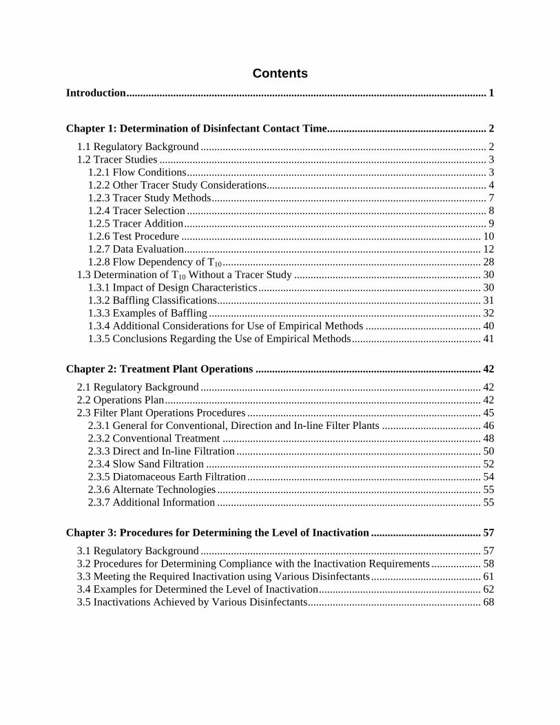
Contents

Introduction ................................................................................................................................... 1

Chapter 1: Determination of Disinfectant Contact Time .......................................................... 2

1.1 Regulatory Background ........................................................................................................ 2 1.2 Tracer Studies ....................................................................................................................... 3

1.2.1 Flow Conditions ............................................................................................................. 3 1.2.2 Other Tracer Study Considerations ................................................................................ 4 1.2.3 Tracer Study Methods .................................................................................................... 7 1.2.4 Tracer Selection ............................................................................................................. 8 1.2.5 Tracer Addition .............................................................................................................. 9 1.2.6 Test Procedure ............................................................................................................. 10 1.2.7 Data Evaluation ............................................................................................................ 12 1.2.8 Flow Dependency of T10 .............................................................................................. 28

1.3 Determination of T10 Without a Tracer Study .................................................................... 30 1.3.1 Impact of Design Characteristics ................................................................................. 30 1.3.2 Baffling Classifications ................................................................................................ 31 1.3.3 Examples of Baffling ................................................................................................... 32 1.3.4 Additional Considerations for Use of Empirical Methods .......................................... 40 1.3.5 Conclusions Regarding the Use of Empirical Methods ............................................... 41

Chapter 2: Treatment Plant Operations .................................................................................. 42

2.1 Regulatory Background ...................................................................................................... 42 2.2 Operations Plan ................................................................................................................... 42 2.3 Filter Plant Operations Procedures ..................................................................................... 45

2.3.1 General for Conventional, Direction and In-line Filter Plants .................................... 46 2.3.2 Conventional Treatment .............................................................................................. 48 2.3.3 Direct and In-line Filtration ......................................................................................... 50 2.3.4 Slow Sand Filtration .................................................................................................... 52 2.3.5 Diatomaceous Earth Filtration ..................................................................................... 54 2.3.6 Alternate Technologies ................................................................................................ 55 2.3.7 Additional Information ................................................................................................ 55

Chapter 3: Procedures for Determining the Level of Inactivation ........................................ 57

3.1 Regulatory Background ...................................................................................................... 57 3.2 Procedures for Determining Compliance with the Inactivation Requirements .................. 58 3.3 Meeting the Required Inactivation using Various Disinfectants ........................................ 61 3.4 Examples for Determined the Level of Inactivation ........................................................... 62 3.5 Inactivations Achieved by Various Disinfectants ............................................................... 68

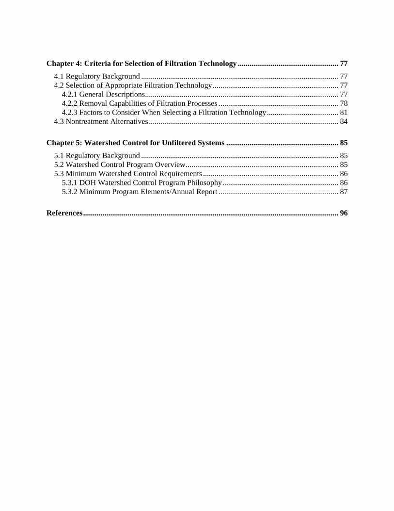
Chapter 4: Criteria for Selection of Filtration Technology .................................................... 77

4.1 Regulatory Background ...................................................................................................... 77 4.2 Selection of Appropriate Filtration Technology ................................................................. 77

4.2.1 General Descriptions .................................................................................................... 77 4.2.2 Removal Capabilities of Filtration Processes .............................................................. 78 4.2.3 Factors to Consider When Selecting a Filtration Technology ..................................... 81

4.3 Nontreatment Alternatives .................................................................................................. 84

Chapter 5: Watershed Control for Unfiltered Systems .......................................................... 85

5.1 Regulatory Background ...................................................................................................... 85 5.2 Watershed Control Program Overview ............................................................................... 85 5.3 Minimum Watershed Control Requirements ...................................................................... 86

5.3.1 DOH Watershed Control Program Philosophy ............................................................ 86 5.3.2 Minimum Program Elements/Annual Report .............................................................. 87

References .................................................................................................................................... 96

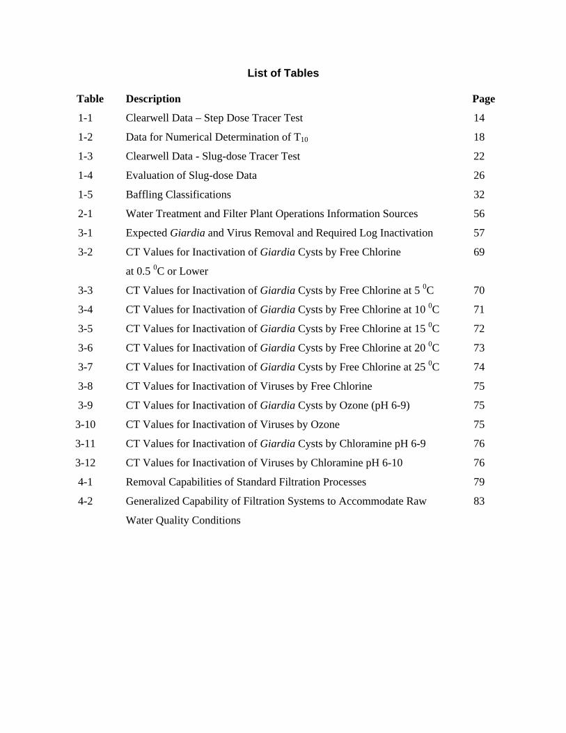
List of Tables

Table Description Page

1-1 Clearwell Data – Step Dose Tracer Test 14

1-2 Data for Numerical Determination of T10 18

1-3 Clearwell Data - Slug-dose Tracer Test 22

1-4 Evaluation of Slug-dose Data 26

1-5 Baffling Classifications 32

2-1 Water Treatment and Filter Plant Operations Information Sources 56

3-1 Expected Giardia and Virus Removal and Required Log Inactivation 57

3-2 CT Values for Inactivation of Giardia Cysts by Free Chlorine

at 0.5 0C or Lower

69

3-3 CT Values for Inactivation of Giardia Cysts by Free Chlorine at 5 0C 70





3-8 CT Values for Inactivation of Viruses by Free Chlorine 75

3-9 CT Values for Inactivation of Giardia Cysts by Ozone (pH 6-9) 75

3-10 CT Values for Inactivation of Viruses by Ozone 75

3-11 CT Values for Inactivation of Giardia Cysts by Chloramine pH 6-9 76

3-12 CT Values for Inactivation of Viruses by Chloramine pH 6-10 76

4-1 Removal Capabilities of Standard Filtration Processes 79

4-2 Generalized Capability of Filtration Systems to Accommodate Raw

Water Quality Conditions

83

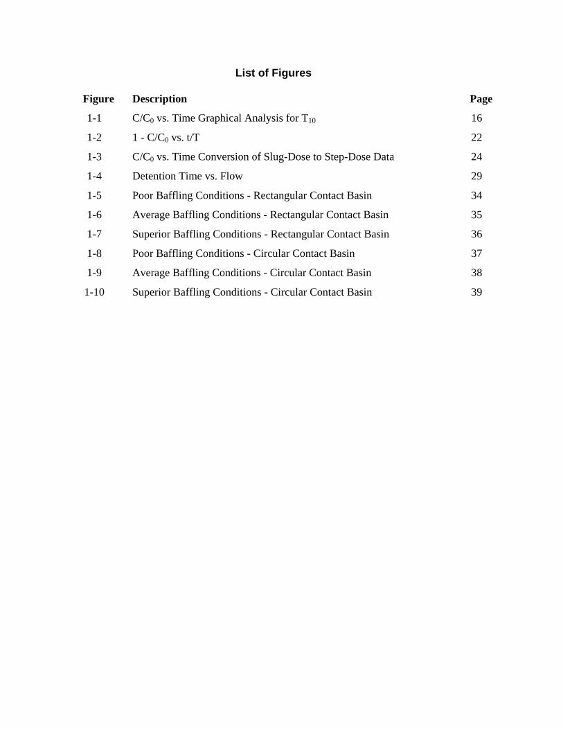
List of Figures

Figure Description Page

1-1 C/C0 vs. Time Graphical Analysis for T10 16

1-2 1 - C/C0 vs. t/T 22

1-3 C/C0 vs. Time Conversion of Slug-Dose to Step-Dose Data 24

1-4 Detention Time vs. Flow 29

1-5 Poor Baffling Conditions - Rectangular Contact Basin 34

1-6 Average Baffling Conditions - Rectangular Contact Basin 35

1-7 Superior Baffling Conditions - Rectangular Contact Basin 36

1-8 Poor Baffling Conditions - Circular Contact Basin 37

1-9 Average Baffling Conditions - Circular Contact Basin 38

1-10 Superior Baffling Conditions - Circular Contact Basin 39

Acronyms

C - residual disinfectant concentration in mg/L

CFR - code of federal regulations

CT - the mathematical product (in mg/L-minutes) of C and T

CTcalc - the CT achieved by a public water system

CTreq'd - the CT value required to achieve a specific log inactivation of

Giardia lamblia cysts or viruses

DE - diatomaceous earth

DOH - Department of Health

gpm - gallons per minute

GWI - groundwater under the direct influence of surface water

MGD - million gallons per day

mg/L - milligrams per liter

NTU - nephelometric turbidity unit

SWTR - Surface Water Treatment Rule

T - disinfectant contact time in minutes

1

Introduction The purpose of this Department of Health (DOH) manual is to provide guidance regarding implementation of the Surface Water Treatment Rule (SWTR) in Washington. The DOH SWTR Guidance Manual is intended for use by public water systems impacted by SWTR and consulting engineers assisting systems with SWTR compliance. Group A systems using surface water or groundwater sources under the direct influence of surface water (GWI) are subject to the SWTR. The DOH SWTR Guidance Manual is designed to complement the surface water treatment requirements found in Part 6 of WAC 246-290, the drinking water regulations. Although a more extensive document was originally planned, due to resource limitations, the content is now limited to the specific topics in which the DOH SWTR Guidance Manual is referenced in Part 6 of the drinking water regulations. For ease of use, chapters are organized in the same order as the DOH SWTR Guidance Manual citations appear in the drinking water regulations. Most of the requirements contained in Part 6 of WAC 246-290 are based on the federal SWTR promulgated June 29, 1989. The Environmental Protection Agency (EPA) has developed an extensive Guidance Manual to complement the federal SWTR. Where appropriate, federal guidance has been directly incorporated into the DOH Guidance Manual. For additional, more detailed guidance regarding SWTR compliance and implementation, systems may refer to the federal SWTR Guidance Manual. Copies of the federal Guidance Manual (document number: PB 93-222-933) are available for a fee ($61 as of April, 1995) from the National Technical Information Service (NTIS). The NTIS toll free number is 1-800-553-6847.

2

Chapter 1: Determination of Disinfectant Contact Time The purpose of this chapter is to provide guidance related to determining contact time in mixing basins, storage reservoirs, etc. The chapter is divided into three sections. The first section provides background on the regulatory requirements for filtered and unfiltered systems as related to contact time determinations. The second section presents a brief synopsis of tracer study methods, procedures, and data evaluation. In addition, examples are presented for conducting hypothetical tracer studies to determine the T10 contact time in a clearwell. The third section presents an empirical method of determining T10 from theoretical detention times in systems where it is impractical or prohibitively expensive to conduct tracer studies. 1.1 Regulatory Background WAC 246-290-636 addresses the SWTR requirements related to contact time determinations. Contact time determinations are important because disinfectant contact time is one of the parameters used by water system operators to assess compliance with the SWTR disinfection requirements. For filtered systems, the level of disinfection required is dependent on the removal credit granted for filtration. The combination of filtration and disinfection must achieve 3 log removal/inactivation of Giardia lamblia cysts and 4 log removal/inactivation of viruses. Systems must on a daily basis determine the level of inactivation achieved using the procedures and CT values (C X T) contained in Chapter 3. As explained in Chapter 3, contact time is needed to compute CT values and ultimately the level of inactivation achieved by disinfection. Unfiltered systems must achieve the 3 log inactivation of Giardia cysts and 4 log inactivation of viruses through disinfection alone. Systems must on a daily basis determine the level of inactivation achieved using the procedures and CT values specified in the Federal Register, 40 CFR 141.74, Volume 54, No. 124 published June 29, 1989. Throughout Part 6, disinfectant contact time is referred to as T. For pipelines, T must be determined through calculations. For all other water system components used for disinfection, such as mixing basins or storage reservoirs, T must be determined through tracer studies or empirical methods. For pipelines, all fluid passing through the pipe is assumed to have a detention time equal to the theoretical or mean residence time at a particular flow rate. Since T must be determined at peak hourly flow, T can be calculated by dividing the internal volume of the pipe by the peak hourly flow rate through the pipe. For mixing basins and storage reservoirs, the contact time which must be used in CT calculations is the detention time at which 90 percent of the water passing through the unit is retained within the basin. This detention time was designated as T10 according to the convention adopted by

3

Thirumurthi (1969). Information provided by tracer studies is used for estimating the detention time, T10. Per WAC 246-290-636(6), under certain circumstances, empirical methods may also be used for estimating T10. 1.2 Tracer Studies 1.2.1 Flow Conditions Although detention time is proportional to flow, it is not generally a linear function. Therefore, tracer studies are needed to establish detention times for the range of flow rates experienced within each disinfectant section. A section is the portion of the system with a measurable contact time between two points of residual monitoring or disinfectant application as discussed in Section 3.2. A single flow rate may not characterize the flow through the entire system. With a series of reservoirs, clearwells, and storage tanks, flow will vary between each portion of the system. In filter plants, the plant flow is relatively uniform from the intake through the filters. An increase or reduction in the intake pumping capacity will impart a proportional change in flow through each process unit prior to and including the filters. Therefore, at a constant intake-pumping rate, flow variations between disinfectant sections within a treatment plant, excluding clearwells, are likely to be small, and the design capacity of the plant, or plant flow, can be considered the nominal flow rate through each individual process unit within the plant. Clearwells may operate at a different flow rate than the rest of the plant, depending on the pumping capacity. Ideally, tracer tests should be performed for at least four flow rates that span the entire range of flow for the section being tested. The flow rates should be separated by approximately equal intervals to span the range of operation; one should be near average flow, two should be greater than average flow, and one less than average flow. The flows should also be selected so that the highest test flow rate is at least 91 percent of the highest flow rate expected to ever occur in that section. Four data points will assure a good definition of the section's hydraulic profile. The results of the tracer tests performed for different flow rates should be used to generate plots of T10 vs. Q for each section in the system. A smooth line is drawn through the points on each graph to create a curve from which T10 may be read for the corresponding Q at peak hourly flow conditions. This procedure is presented in Section 1.2.8. It may not be practical for all systems to conduct studies at four flow rates. The number of tracer tests that are practical to conduct is dependent on site-specific restrictions and resources available to the system. Systems with limited resources can conduct a minimum of one tracer test for each disinfectant section at a flow rate of not less than 91 percent of the highest flow rate experienced at that section. If only one tracer test is performed, the detention time determined by the test may be used to provide a conservative estimate in CT calculations for that section for all flow rates less than or equal to the tracer test flow rate.

4

The detention time, T10, is inversely proportional to flow rate. Therefore, the T10 at a flow rate other than that which the tracer study was conducted (T10S) can be determined by multiplying the T10 from the tracer study (T10T) by the ratio of the tracer study flow rate to the desired flow rate as follows:

T10S = T10T X QT where: QD

T10S = T10 at system flow rate T10T = T10 at tracer flow rate QT = Tracer study flow rate QD = System flow rate

The most accurate tracer test results are obtained when flow is constant through the section during the course of the test. Therefore, the tracer study should be conducted at a constant flow whenever practical. For a treatment plant consisting of two or more equivalent process trains, a constant flow tracer test can be performed on a section of the plant by holding the flow through one of the trains constant while operating the parallel train(s) to absorb any flow variations. Flow variations during tracer tests in systems without parallel trains or with single clearwells and storage reservoirs are more difficult to avoid. In these instances, T10 should be recorded at the average flow rate over the course of the test. 1.2.2 Other Tracer Study Considerations In addition to flow conditions, detention times determined by tracer studies are dependent on the water level in the contact basin. This is particularly pertinent to storage tanks, reservoirs, and clearwells which, in addition to being contact basins for disinfection, are also often used as equalization storage for distribution system demands. In such instances, the water levels in the reservoirs vary to meet the system demands. The actual detention time of these contact basins will also vary depending on whether they are emptying or filling. For some process units, especially sedimentation basins which are operated at a near constant level, that is, flow in equals flow out, the detention time determined by tracer tests is valid for calculating CT when the basin is operating at water levels greater than or equal to the level at which the test was performed. If the water level during testing is higher than the normal operating level, the resulting concentration profile will predict an erroneously high detention time. Conversely, extremely low water levels during testing may lead to an overly conservative detention time. Therefore, when conducting a tracer study to determine the detention time, a water level at or slightly below, but not above, the normal minimum operating level is recommended.

5

For many plants, the water level in a clearwell or storage tank varies between high and low levels in response to distribution system demands. In such instances, to obtain a conservative estimate of the contact time, the tracer study should be conducted during a period when the tank level is falling (flow out greater than flow in). This procedure will provide a detention time for the contact basin which is also valid when the water level is rising (flow out less than flow in) from a level which is at or above the level when the T10 was determined by the tracer study. Whether the water level is constant or variable, the tracer study for each section should be repeated for several different flows, as described in the Section 1.2.1. For clearwells that are operated with extreme variations in water level, maintaining a CT to comply with inactivation requirements may be impractical. Under such operating conditions, a reliable detention time is not provided for disinfection. However, the system may install a weir to ensure a minimum water level and provide a reliable detention time. Systems comprised of storage reservoirs that experience seasonal variations in water levels may perform tracer studies during the various seasonal conditions. For these systems, tracer tests should be conducted at several flow rates and representative water levels that occur for each seasonal condition. The results of these tests can be used to develop hydraulic profiles of the reservoir for each water level. These profiles can be plotted on the same axis of T10 vs. Q and may be used for calculating CT for different water levels and flow rates. Detention time may also be influenced by differences in water temperature within the system. For plants with potential for thermal stratification, additional tracer studies are suggested under the various seasonal conditions which are likely to occur. The contact times determined by the tracer studies under the various seasonal conditions should remain valid as long as no physical changes are made to the mixing basin(s) or storage reservoir(s). As stated previously (Section 1.2.1), the portion of the system with a measurable contact time between two points of disinfection or residual monitoring is referred to as a section. For systems which apply disinfectant(s) at more than one point, or choose to profile the residual from one point of application, tracer studies should be conducted to determine T10 for each section containing process unit(s). The T10 for a section may or may not include a length of pipe and is used along with the residual disinfectant concentration prior to the next disinfectant application or monitoring point to determine the CTcalc for that section. The inactivation ratio for the section is then determined. The total inactivation ratio achieved by the system can then be determined by summing the inactivation ratios for all sections as explained in Chapter 3. For systems that have two or more units of identical size and configuration, tracer studies only need to be conducted on one of the units. The resulting graph of T10 vs. flow can be used to determine T10 for all identical units. Systems with more than one section in the treatment plant may determine T10 for each section by:

o Individual tracer studies through each section; or o One tracer study across the system.

6

If possible, individual tracer studies should be conducted on each section. To minimize the time needed to conduct studies on each section, the tracer studies should be started at the last section of the treatment train prior to the first customer and completed with the first section of the system. Conducting the tracer studies in this order will prevent the interference of residual tracer material with subsequent studies. However, it may not always be practical for systems to conduct tracer studies for each section because of time and manpower constraints. In these cases, one tracer study may be used to determine the T10 values for all of the sections at one flow rate. This procedure involves the following steps:

1. Add tracer at the beginning of the furthest upstream disinfection section. 2. Measure the tracer concentration at the end of each disinfection section. 3. Determine the T10 to each monitoring point as outlined in the data evaluation examples

presented in Section 1.2.7. 4. Subtract T10 values of each of the upstream sections from the overall T10 value to

determine the T10 of each downstream section. This approach is valid for a series of two or more consecutive sections as long as all process units within the sections experience the same flow condition. This approach is illustrated by Hudson (1975) in which step-dose tracer tests were employed to evaluate the baffling characteristics of flocculators and settling basins at six water treatment plants. At one plant, tracer chemical was added to the rapid mix, which represented the beginning of the furthest upstream disinfection section in the system. Samples were collected from the flocculator and settling basin outlets and analyzed to determine the residence-time characteristics for each section. Tracer measurements at the flocculator outlet indicated an approximate T10 of 5 minutes through the rapid mix, interbasin piping and flocculator. Based on tracer concentration monitoring at the settling basin outlet, an approximate T10 of 70 minutes was determined for the combined sections, including the rapid mix, interbasin piping, flocculator, and settling basin. The flocculator T10 of 5 minutes was subtracted from the combined sections' T10 of 70 minutes, to determine the T10 for the settling basin alone, 65 minutes. This approach may also be applied in cases where disinfectant application and/or residual monitoring is discontinued at any point between two or more sections with known T10 values. These T10 values may be summed to obtain an equivalent T10 for the combined sections. For ozone contactors, flocculators or any basin containing mixing, tracer studies should be conducted for the range of mixing used in the process. In ozone contactors, air or oxygen should be added in lieu of ozone to prevent degradation of the tracer. The flow rate of air or oxygen used for the contactor should be applied during the study to simulate actual operation. Tracer studies should then be conducted at several air/oxygen to water ratios to provide data for the complete range of ratios used at the plant. For flocculators, tracer studies should be conducted for various mixing intensities to provide data for the complete range of operations.

7

1.2.3 Tracer Study Methods This section discusses the two most common methods of tracer addition employed in water treatment evaluations, the step-dose method and the slug-dose method. Tracer study methods involve the application of chemical dosages to a system and tracking the resulting effluent concentration as a function of time. The effluent concentration profile is evaluated to determine the detention time, T10, used in CT calculations. While both tracer test methods can use the same tracer materials and involve measuring the concentration of tracer with time, each has distinct advantages and disadvantages with respect to tracer addition procedures and analysis of results. The step-dose method entails introduction of a tracer chemical at a constant dosage until the concentration at the desired end point reaches a steady-state level. Step-dose tracer studies are frequently employed in drinking water applications for the following reasons:

o The resulting normalized concentration vs. time profile is directly used to determine, T10, the detention time required for calculating CT; and

o Very often, the necessary feed equipment is available to provide a constant rate of

application of the tracer chemical. One other advantage of the step-dose method is that the data may be verified by comparing the concentration versus elapsed time profile for samples collected at the start of dosing with the profile obtained when the tracer feed is discontinued. Alternatively, with the slug-dose method, a large instantaneous dose of tracer is added to the incoming water and samples are taken at the exit of the unit over time as the tracer passes through the unit. A disadvantage of this technique is that very concentrated solutions are needed for the dose to adequately define the concentration versus time profile. Intensive mixing is therefore required to minimize potential density-current effects and to obtain a uniform distribution of the instantaneous tracer dose across the basin. This is inherently difficult under water flow conditions often existing at inlets to basins. Other disadvantages of using the slug-dose method include:

o The concentration and volume of the instantaneous tracer dose must be carefully computed to provide an adequate tracer profile at the effluent of the basin;

o The resulting concentration vs. time profile cannot be used to directly determine T10

without further manipulation; and

o A mass balance on the treatment section is required to determine whether the tracer was completely recovered.

8

One advantage of this method is that it may be applied where chemical feed equipment is not available at the desired point of addition, or where the equipment available does not have the capacity to provide the necessary concentration of the chosen tracer chemical. Although, in general, the step-dose procedure offers the greatest simplicity, both methods are theoretically equivalent for determining T10. Either method is acceptable for conducting drinking water tracer studies, and the choice of the method should be determined by site-specific constraints or the system's experience.

1.2.4 Tracer Selection An important step in any tracer study is the selection of a tracer chemical. Ideally, the selected chemical should be readily available, conservative (not consumed or removed during treatment), easily monitored, and acceptable for potable water use. In general to be considered acceptable for potable water use, a chemical shall be listed under ANSI/NSF Standard 60 by an ANSI-accredited listing agency (per the DOH Drinking Water Additives Policy). Use of other chemicals will be considered on a case-by-case basis. Historically, tracer chemicals not satisfying all these criteria have been used including potassium permanganate, alum, chlorine, and sodium carbonate. Chloride and fluoride are the most common tracer chemicals employed in drinking water plants that are nontoxic and approved for potable water use. Rhodamine WT can be used as a fluorescent tracer in water flow studies in accordance with the following guidelines:

o Raw water concentrations should be limited to a maximum concentration of 10 mg/L and drinking water concentrations should not exceed 0.1 ug/L.

o Studies which result in human exposure to the dye must be brief and infrequent.

o Concentrations as low as 2 ug/L can be used in tracer studies because of the low

detection level (in the range of 0.1 to 0.2 ug/L). The use of Rhodamine B as a tracer in water flow studies is not recommended by the EPA nor DOH. The choice of a tracer chemical can be made based, in part, on the selected dosing method and also on the availability of chemical feeding equipment. For example, the high density of concentrated salt solutions and their potential for inducing density currents usually precludes chloride and fluoride as the selected chemical for slug-dose tracer tests. Fluoride can be a convenient tracer chemical for step-dose tracer tests of clearwells because it is frequently applied for finished water treatment. However, when fluoride is used in tracer tests on clarifiers, allowances should be made for fluoride that is absorbed on floc and settles out of water (Hudson, 1975).

9

Additional considerations when using fluoride in tracer studies include:

o It is difficult to detect at low levels;

o State drinking water regulations impose a finished water concentration range of 0.8 through 1.3 mg/L; and

o The secondary and primary drinking water standards (MCLs) for fluoride are 2 and 4

mg/L, respectively. For safety reasons, the use of fluoride is only recommended in cases where the feed equipment is already in place. In instances where only one of two (or more) parallel units is tested, flow from the other unit(s) may dilute the tracer concentration prior to leaving the plant and entering the distribution system. Therefore, the impact of drinking water standards on the use of fluoride and other tracer chemicals can be alleviated in some cases. 1.2.5 Tracer Addition The tracer chemical should be added at the same point(s) in the treatment train as the application points of the disinfectant to be used in the CT calculations. 1.2.5.1 Step-dose Method The duration of tracer addition is dependent on the volume of the basin, and hence, its theoretical detention time. To approach a steady-state concentration in the water exiting the basin, tracer addition and sampling should usually be continued for a period of two to three times the theoretical detention time (Hudson, 1981). It is not necessary to reach a steady state concentration in the exiting water to determine T10; however, it is necessary to determine tracer recovery. It is recommended that the tracer recovery be determined to identify hydraulic characteristics or density problems. In all cases, the tracer chemical should be dosed in sufficient concentration to easily monitor a residual at the basin outlet throughout the test. The required tracer chemical concentration is generally dependent upon the nature of the chosen tracer chemical (including its background concentration) and the mixing characteristics of the basin to be tested. Recommended chloride doses on the order of 20 mg/L (Hudson, 1975) should be used for step-dose method tracer studies where the background chloride level is less than 10 mg/L. Also, fluoride concentrations as low as 1.0 to 1.5 mg/L are practical when the raw water fluoride level is not significant (Hudson, 1975). However, tracer studies conducted on systems suffering from serious short-circuiting of flow (actual detention time is much less than theoretical detention time due to unbaffled in) may require substantially larger step-doses. This would be necessary to detect the tracer chemical and to adequately define the effluent tracer concentration profile.

10

1.2.5.2 Slug-dose Method The duration of tracer measurements using the slug-dose method is also dependent on the volume of the basin, and hence, its theoretical detention time. In general, samples should be collected for a period of at least twice the basin's theoretical detention time, or until tracer concentrations are detected near background levels. To get reliable results for T10 values using the slug-dose method, it is recommended that the total mass of tracer recovered be approximately 90 percent of the mass applied. This guideline presents the need to sample until the tracer concentration recedes to the background level. The total mass recovered during testing will not be known until completion of the testing and analysis of the data collected. The sampling period needed is very site-specific. Therefore, it may be helpful to conduct a first run tracer test as a screen to identify the appropriate sampling period for gathering data to determine T10. Tracer addition for slug-dose method tests should be instantaneous and provide uniformly mixed distribution of the chemical. Tracer addition is considered instantaneous if the dosing time does not exceed 2 percent of the basin's theoretical detention time (Marske and Boyle, 1973). One recommended procedure for achieving instantaneous tracer dosing is to apply the chemical by gravity flow through a funnel and hose apparatus. This method is also beneficial since it provides a means of standardization (which is necessary to obtain reproducible results). The mass of tracer chemical to be added is determined by the desired theoretical concentration and basin size. The mass of tracer added in slug-dose tracer tests should be the minimum mass needed to obtain detectable residual measurements to generate a concentration profile. As a guideline, the theoretical concentration for the slug-dose method should be comparable to the constant dose applied in step-dose tracer tests (10 to 20 mg/L and 1 to 2 mg/L for chloride and fluoride, respectively). The mass of tracer chemical is calculated by multiplying the theoretical concentration by the total basin volume. This is appropriate for systems with high dispersion and/or mixing. This quantity is diluted as required to apply an instantaneous dose and minimize density effects. It should be noted that the mass applied is not likely to get completely mixed throughout the total volume of the basin. Therefore, the detected concentration might exceed theoretical concentrations based on the total volume of the basin. For these cases, the mass of chemical to be added can be determined by multiplying the theoretical concentration by only a portion of the basin volume. An example of this is shown in Section 1.2.7.2 for a slug-dose tracer study. In cases where the tracer concentration in the effluent must be maintained below a specified level, it may be necessary to conduct a preliminary test run with a minimum tracer dose to identify the appropriate dose for determining T10 without exceeding this level. 1.2.6 Test Procedure In preparation for beginning a tracer study, the raw water background concentration of the chosen tracer chemical must be established. The background concentration is essential, not only

11

for aiding in the selection of the tracer dosage, but also to facilitate proper evaluation of the data. The background tracer concentration should be determined by monitoring for the tracer chemical prior to beginning the test. The sampling point(s) for the pre-tracer study monitoring should be the same as the points to be used for residual monitoring to determine CT values. The monitoring procedure is outlined in the following steps:

1. If the tracer chemical is normally added for treatment, discontinue its addition to the water in sufficient time to permit the tracer concentration to recede to its background level before the test is begun.

2. Prior to the start of the test, regardless of whether the chosen tracer material is a treatment chemical, monitor the tracer concentration in the water at the sampling point where the disinfectant residual will be measured for CT calculations.

3. If a background tracer concentration is detected, monitor it until a constant concentration, at or below the raw water background level, is achieved. This measured concentration is the baseline tracer concentration.

Following the determination of the tracer dosage, feed and monitoring point(s) and a baseline tracer concentration, tracer testing can begin. Equal sampling intervals, as could be obtained from automatic sampling, are not required for either tracer study method. However, using equal sample intervals for the slug-dose method can simplify the analysis of the data. During testing, the time and tracer residual of each measurement should also be recorded on a data sheet. In addition, the water level, flow, and temperature should be recorded during the test. 1.2.6.1 Step-dose Method At time zero, the tracer chemical feed will be started and left at a constant rate for the duration of the test. Over the course of the test, the tracer residual should be monitored at the required sampling point(s) at a frequency determined by the overall detention time and site-specific considerations. As a general guideline, sampling at intervals of 2 to 5 minutes should provide data for a well-defined plot of tracer concentration versus time. If on-site analysis is available, less frequent residual monitoring may be possible until a change in residual concentration is first detected. As a guideline, in systems with a theoretical detention time greater than 4 hours, sampling may be conducted every 10 minutes for the first 30 minutes, or until a tracer concentration above the baseline level is first detected. In general, shorter sampling intervals enable better characterization of concentration changes; therefore, sampling should be conducted at 2 to 5-minute intervals from the time that a concentration change is first observed until the residual concentration reaches a steady-state value. A reasonable sampling interval should be chosen based on the overall detention time of the unit being tested.

12

If verification of the test is desired, the tracer feed should be discontinued, and the receding tracer concentration at the effluent should be monitored at the same frequency until tracer concentrations corresponding to the background level are detected. The time at which tracer feed is stopped is time zero for the receding tracer test and must be noted. The receding tracer test will provide a replicate set of measurements which can be compared with data derived from the rising tracer concentration versus time curve. For systems which currently feed the tracer chemical, the receding curve may be generated from the time the feed is turned off to determine the background concentration level. 1.2.6.2 Slug-dose Method At time zero for the slug-dose method, a large instantaneous dose of tracer will be added to the influent of the unit. The same sampling locations and frequencies described for step-dose method tests also apply to slug-dose method tracer studies. One exception with this method is that the tracer concentration profile will not equilibrate to a steady state concentration. Because of this, the tracer should be monitored frequently enough to ensure acquisition of data needed to identify the peak tracer concentration. Slug-dose method tests should be checked by performing a material balance to ensure that all of the tracer fed is recovered, i.e. mass applied equals mass discharged. 1.2.7 Data Evaluation Data from tracer studies should be summarized in tables of time and residual concentration. These data are then analyzed to determine the detention time, T10, to be used in calculating CT. Tracer test data from either the step or slug-dose method can be evaluated graphically, numerically, or by a combination of these techniques. 1.2.7.1 Step-dose Method The graphical method of evaluating step-dose test data involves plotting a graph of dimensionless concentration versus time and reading the value for T10 directly from the graph at the appropriate dimensionless concentration. Alternatively, the data from step-dose tracer studies may be evaluated numerically by developing a semi-logarithmic plot of the dimensionless data. The semi-logarithmic plot allows a straight line to be drawn through the data. The resulting equation of the line is used to calculate the T10 value, assuming that the correlation coefficient indicates a good statistical fit (0.9 or above). Scattered data points from step-dose tracer tests are discredited by drawing a smooth curve through the data. An illustration of the T10 determination is presented in the example (starting on page 15) of the data evaluation required for a clearwell tracer study.

13

1.2.7.2 Slug-dose Method Data from slug-dose tracer tests is analyzed by converting it to the mathematically equivalent step-dose data and using techniques discussed in Section 1.2.7.1 to determine T10. A graph of dimensionless concentration versus time should be drawn which represents the results of a slug-dose tracer test. The key to converting between the data forms is obtaining the total area under the slug-dose data curve. This area is found by graphically or numerically integrating the curve. The conversion to step-dose data is then completed in several mathematical steps involving the total area. A graphical technique for converting the slug-dose data to step-dose data involves physically measuring the area under the curve using a planimeter. The planimeter is an instrument used to measure the area of a plane closed curve by tracing its boundary. Calibration of this instrument to the scale of the graph is required to obtain meaningful readings. A simple numerical integration method is the "rectangle rule" which approximates the total area under the curve as the sum of the areas of individual rectangles. These rectangles have heights and widths equal to the residual concentration and sampling interval (time) for each data point on the curve, respectively. Once the data has been converted, T10 may be determined in the same manner as data from step-dose tracer tests. Slug-dose concentration profiles can have many shapes, depending on the hydraulics of the basin. Therefore, slug-dose data points should not be discredited by drawing a smooth curve through the data prior to its conversion to step-dose data. The steps and specific details involved with evaluating data from both tracer study methods are illustrated in the following example. Example: Determining T10 in a Clearwell Using Step-dose and Slug-dose Methods Two tracer studies employing the step-dose and slug-dose methods of tracer addition were conducted for a clearwell with a theoretical detention time, T, of 30 minutes at an average flow of 2.5 MGD. Because fluoride is added at the inlet to the clearwell as a water treatment chemical, necessary feed equipment was in place for dosing a constant concentration of fluoride throughout the step-dose tracer test. Based on this convenience, fluoride was chosen as the tracer chemical for the step-dose method test. Fluoride was also selected as the tracer chemical for the slug-dose method test. Prior to the start of testing, a fluoride baseline concentration of 0.2 mg/L was established for the water exiting the clearwell. Tracer Study 1: Step-dose Method Test For the step-dose test a constant fluoride dosage of 2.0 mg/L was added to the clearwell inlet. Fluoride levels in the clearwell effluent were monitored and recorded every 3 minutes. The raw tracer study data, along with the results of further analyses, are shown in Table 1-1.

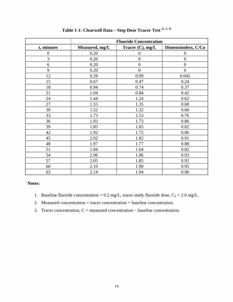
14

Table 1-1: Clearwell Data – Step Dose Tracer Test (1, 2, 3) Fluoride Concentration

t, minutes Measured, mg/L Tracer (C), mg/L Dimensionless, C/Co 0 0.20 0 0 3 0.20 0 0 6 0.20 0 0 9 0.20 0 0 12 0.29 0.09 0.045 15 0.67 0.47 0.24 18 0.94 0.74 0.37 21 1.04 0.84 0.42 24 1.44 1.24 0.62 27 1.55 1.35 0.68 30 1.52 1.32 0.66 33 1.73 1.53 0.76 36 1.93 1.73 0.86 39 1.85 1.65 0.82 42 1.92 1.72 0.86 45 2.02 1.82 0.91 48 1.97 1.77 0.88 51 1.84 1.64 0.82 54 2.06 1.86 0.93 57 2.05 1.85 0.92 60 2.10 1.90 0.95 63 2.14 1.94 0.96

Notes:

1. Baseline fluoride concentration = 0.2 mg/L, tracer study fluoride dose, C0 = 2.0 mg/L.

2. Measured concentration = tracer concentration + baseline concentration.

3. Tracer concentration, C = measured concentration – baseline concentration.

15

The steps in evaluating the raw data shown in the first column of Table 1-1 are as follows. First, the baseline fluoride concentration, 0.2 mg/L, is subtracted from the measured concentration to give the fluoride concentration resulting from the tracer study addition alone. For example, at elapsed time = 39 minutes, the tracer fluoride concentration, C, is obtained as follows:

C = Cmeasured – Cbaseline = 1.85 mg/L - 0.2 mg/L = 1.65 mg/L

This calculation was repeated at each time interval to obtain the data shown in the third column of Table 1-1. As indicated, the fluoride concentration rises from 0 mg/L at t = 0 minutes to the applied fluoride dosage of 2 mg/L at t = 63 minutes. The next step is to develop dimensionless concentrations by dividing the tracer concentrations in the second column of Table 1-1 by the applied fluoride dosage, Co (i.e. 2 mg/L). For time = 39 minutes, C/Co is calculated as follows:

C/Co = (1.65 mg/L)/(2.0 mg/L)

= 0.82 The resulting dimensionless data, presented in the fourth column of Table 1-1, is the basis for completing the determination of T10 by either the graphical or numerical method. Graphical Method In order to determine T10 by the graphical method, a plot of C/Co vs. time should be generated using the data in Table 1-1. A smooth curve should be drawn through the data as shown on Figure 1-1. T10 is read directly from the graph at a dimensionless concentration (C/Co) corresponding to the time for which 10 percent of the tracer has passed at the effluent end of the contact basin (T10). For step-dose method tracer studies, this dimensionless concentration is C/Co = 0.10 (Levenspiel, 1972). T10 should be read directly from Figure 1-1 at C/Co = 0.1 by first drawing a horizontal line (C/Co = 0.1) from the Y-axis (t = 0) to its intersection with the smooth curve drawn through the data. At this point of intersection, the time read from X-axis is T10 and may be found by extending a vertical line downward to the X-axis. These steps were performed as illustrated on Figure 1-1 resulting in a value of T10 of approximately 13 minutes.

17

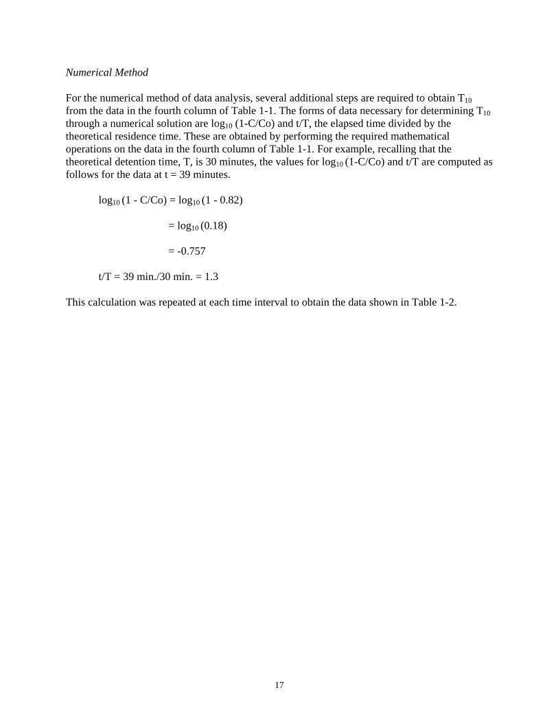
Numerical Method For the numerical method of data analysis, several additional steps are required to obtain T10 from the data in the fourth column of Table 1-1. The forms of data necessary for determining T10 through a numerical solution are log10 (1-C/Co) and t/T, the elapsed time divided by the theoretical residence time. These are obtained by performing the required mathematical operations on the data in the fourth column of Table 1-1. For example, recalling that the theoretical detention time, T, is 30 minutes, the values for log10 (1-C/Co) and t/T are computed as follows for the data at t = 39 minutes.

log10 (1 - C/Co) = log10 (1 - 0.82)

= log10 (0.18) = -0.757

t/T = 39 min./30 min. = 1.3

This calculation was repeated at each time interval to obtain the data shown in Table 1-2.

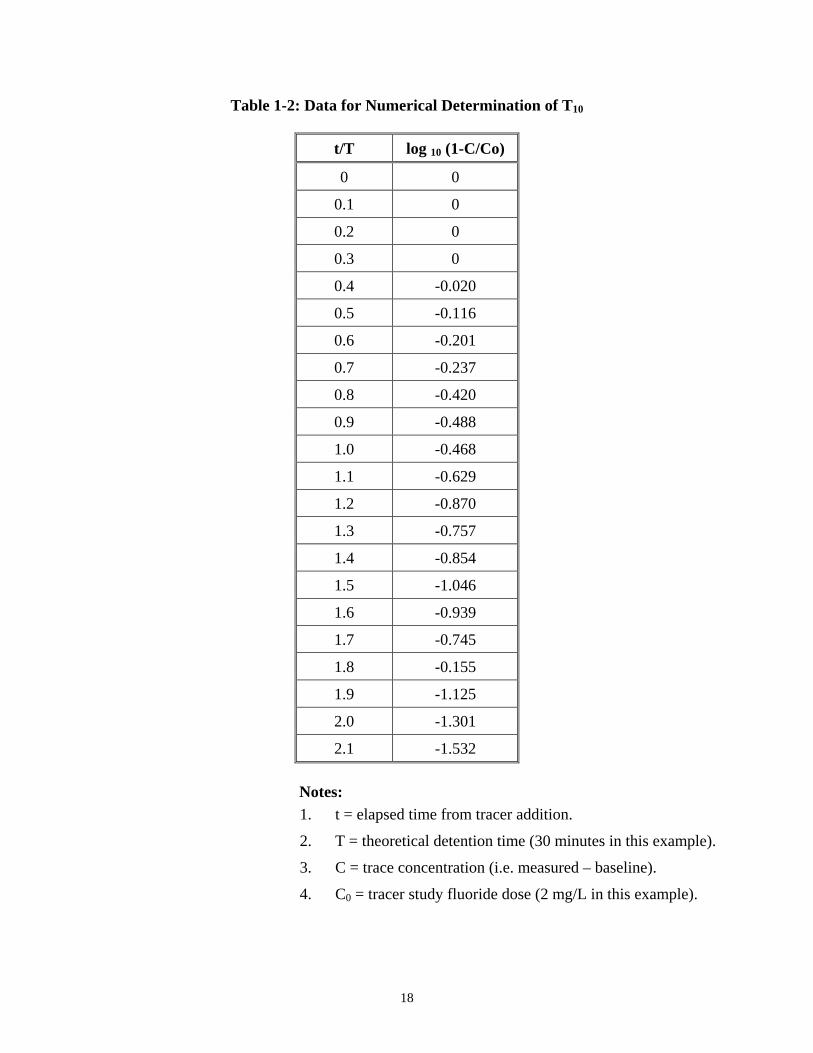
18

Table 1-2: Data for Numerical Determination of T10

t/T log 10 (1-C/Co)

0 0

0.1 0

0.2 0

0.3 0

0.4 -0.020

0.5 -0.116

0.6 -0.201

0.7 -0.237

0.8 -0.420

0.9 -0.488

1.0 -0.468

1.1 -0.629

1.2 -0.870

1.3 -0.757

1.4 -0.854

1.5 -1.046

1.6 -0.939

1.7 -0.745

1.8 -0.155

1.9 -1.125

2.0 -1.301

2.1 -1.532

Notes: 1. t = elapsed time from tracer addition.

2. T = theoretical detention time (30 minutes in this example).

3. C = trace concentration (i.e. measured – baseline).

4. C0 = tracer study fluoride dose (2 mg/L in this example).

19

These data in Table 1-2 should be linearly regressed as log10(1-C/Co) versus t/T to obtain the fitted straight-line parameters to the following equation:

log10 (1-C/Co) = m(t/T) + b (1) In equation 1, m and b are the slope and intercept, respectively, for a plot of log10 (1-C/Co) vs. t/T. This equation can be used to calculate T10, assuming that the correlation coefficient for the fitted data indicates a good statistical fit (0.9 or above). A linear regression analysis was performed on the data in Table 1-2, resulting in the following straight-line parameters:

slope, m = -0.774 intercept, b = 0.251 correlation coefficient = 0.93

Although these numbers were obtained numerically, a plot of log10 (1-C/Co) versus t/T is shown for illustrative purposes on Figure 1-2 for the data in Table 1-2. In this analysis, data for time = 0 through 9 minutes were excluded because fluoride concentrations above the baseline level were not observed in the clearwell effluent until t = 12 minutes. Equation 1 is then rearranged in the following form to facilitate a solution for T10:

T10/T = [log10(1 - 0.1) - b]/m (2) In equation 2, as with graphical method, T10 is determined at the time for which C/Co = 0.1. Therefore, in equation 2, C/Co has been replaced by 0.1 and t (time) by T10. To obtain a solution for T10, the values of the slope, intercept, and theoretical detention time are substituted as follows:

T10/30 min. = [log10 (1 - 0.1) - 0.251]/(-0.774)

T10 = 12 minutes In summary, both the graphical and numerical methods of data reduction resulted in comparable values for T10.

21

Trace Study 2: Slug-dose Method Test A slug-dose tracer test was also performed on the clearwell at a flow rate of 2.5 MGD. A theoretical clearwell fluoride concentration of 2.2 mg/L was selected based on the baseline fluoride concentration of 0.2 mg/L, and to maintain the finished water fluoride level below 2 mg/L. The fluoride dosing volume and concentration were determined from the following considerations: Dosing Volume The fluoride injection apparatus consisted of a funnel and a length of copper tubing. This apparatus provided a constant volumetric feeding rate of 7.5 liters per minute (L/min) under gravity flow conditions. At a flow rate of 2.5 MGD, the clearwell has a theoretical detention time of 30 minutes. Since the duration of tracer injection should be less than 2 percent of the clearwell's theoretical detention time for an instantaneous dose, the maximum duration of fluoride injection was:

Max. dosing time = 30 minutes x 0.02 = 0.6 minutes At a dosing rate of 7.5 L/min, the maximum fluoride dosing volume is calculated to be:

Max. dosing volume = 7.5 L/min. x 0.6 minutes = 4.5 L For this tracer test, a dosing volume of 4 liters was selected, providing an instantaneous fluoride dose in 1.8 percent of the theoretical detention time. Fluoride Concentration The theoretical detention time of the clearwell, T = 30 minutes, was calculated by dividing the clearwell volume of 52,100 gallons (or 197,200 liters) by the average flow rate through the clearwell, i.e. 2.5 MGD. The mass of fluoride required to achieve a theoretical concentration of 2.2 mg/L is calculated as follows:

Fluoride mass (initial) = 2.2 mg/L x 197,200 L x 1 g 1000 mg

= 434 g

22

The concentration of the instantaneous fluoride dose is determined by dividing this mass by the dosing volume, 4 liters:

Fluoride concentration = 434 g 4 L

= 109 g/L

Fluoride levels in the exit to the clearwell were monitored and recorded every 3 minutes. The raw slug-dose tracer test data are shown in Table 1-3.

Table 1-3: Clearwell Data – Slug-dose Tracer Test (1, 2, 3) Fluoride Concentration

t, minutes Measured, mg/L Tracer (C), mg/L Dimensionless, C/Co 0 0.2 0 0 3 0.2 0 0 6 0.2 0 0 9 0.2 0 0 12 1.2 1 0.45 15 3.6 3.4 1.55 18 3.8 3.6 1.64 21 2.0 1.8 0.82 24 2.1 1.9 0.86 27 1.4 1.2 0.55 30 1.3 1.1 0.50 33 1.5 1.3 0.59 36 1.0 0.8 0.36 39 0.6 0.4 0.18 42 1.0 0.8 0.36 45 0.6 0.4 0.18 48 0.8 0.6 0.27 51 0.6 0.4 0.18 54 0.4 0.2 0.09 57 0.5 0.3 0.14 60 0.6 0.4 0.18 63 0.4 0.2 0.09

Notes: 1. Measured concentration = tracer concentration + baseline concentration.

2. Baseline concentration = 0.2 mg/Lm fluoride dose = 109 g/L, theoretical fluoride concentration, C0.

3. Tracer concentration, C = measured concentration – baseline concentration.

23

The first step in evaluating the data for different times is to subtract the baseline fluoride concentration, 0.2 mg/L, from the measured concentration at each sampling interval (Table 1-3). This is the same as the first step used to evaluate step-dose method data and gives the fluoride concentrations resulting from the tracer addition alone, shown in the third column of Table 1-3. As indicated, the fluoride concentration rises from 0 mg/L at t = 0 minutes to the peak concentration of 3.6 mg/L at t = 18 minutes. The exiting fluoride concentration gradually recedes to near zero at t = 63 minutes. The dimensionless concentrations in the fourth column of Table 1-3 were obtained by dividing the tracer concentrations in the third column by the clearwell's theoretical fluoride concentration, Co = 2.2 mg/L. These dimensionless concentrations were then plotted as a function of time, as is shown by the slug-dose data on Figure 1-3. These data points were connected by straight lines, resulting in a somewhat jagged curve.

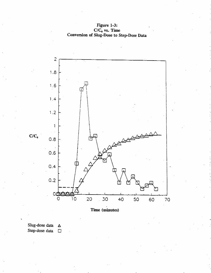
25

The next step in evaluating slug-dose data is to determine the total area under the slug-dose data curve on Figure 1-3. As with the step-dose data evaluation, two methods exist for finding this area: graphical and numerical. As mentioned previously, the graphical method is based on a physical measurement of the area using a planimeter. This involves calibration of the instrument to define the units conversion and tracing the outline of the curve to determine the area. The results of performing this procedure may vary depending on instrument accuracy and measurement technique. Therefore, only an illustration of the numerical technique for finding the area under the slug-dose curve will be presented for this example. However, the area obtained by either the graphical or numerical method would be similar. Furthermore, once the area is found, the remaining steps involved with converting the data to the step-dose response are the same. Table 1-4 summarizes the results of determining the total area using the numerical integration technique called the rectangle rule. The first and second columns in Table 1-4 are the sampling time and fluoride concentration resulting from tracer addition alone, respectively. The steps in applying these data are as follows. First, the sampling time interval, 3 minutes, is multiplied by the fluoride concentration at the end of the 3-minute interval to give the incremental area, in units of milligram minutes per liter. For example, at elapsed time, t = 39 minutes, the incremental area is obtained as follows:

Incremental Area = sampling time interval x fluoride concentration

= (39-36) minutes x 0.4 mg/L

= 1.2 mg-min/L

This calculation was repeated at each time interval to obtain the data shown in the third column of Table 1-4.

26

Table 1-4: Evaluation of Slug-dose Data

t, minutes Fluoride, mg/L Incremental Area, mg-min/L Cumulative Area, mg-min/L Equivalent Step-dose Data 0 0 0 0 0 3 0 0 0 0 6 0 0 0 0 9 0 0 0 0 12 1 3 3 0.05 15 3.4 10.2 13.2 0.22 18 3.6 10.8 24.0 0.40 21 1.8 5.4 29.4 0.49 24 1.9 5.7 35.1 0.59 27 1.2 3.6 38.7 0.65 30 1.1 3.3 42.0 0.71 33 1.3 3.9 45.9 0.77 36 0.8 2.4 48.3 0.81 39 0.4 1.2 49.5 0.83 42 0.8 2.4 51.9 0.87 45 0.4 1.2 53.1 0.89 48 0.6 1.8 54.9 0.92 51 0.4 1.2 56.1 0.94 54 0.2 0.6 56.7 0.95 57 0.3 0.9 57.6 0.97 60 0.4 1.2 58.8 0.99 63 0.2 + 0.6 59.4 1.00 Total Area = 59.4

27

If the data had been obtained at unequal sampling intervals, then the incremental area for each interval would be obtained by multiplying the fluoride concentration at the end of each interval by the time duration of the interval. This convention also requires that the incremental area be zero at the first sampling point, regardless of the fluoride concentration at that time. As is shown in Table 1-4, all incremental areas were summed to obtain 59.4 mg-min/L, the total area under the slug-dose tracer test curve. This number represents the total mass of fluoride that was detected during the course of the tracer test divided by the average flow rate through the clearwell. To complete the conversion of slug-dose data to its equivalent step-dose response requires two additional steps. The first involves summing, consecutively, the incremental areas in the third column of Table 1-4 to obtain the cumulative area at the end of each sampling interval. The cumulative area at time, t = 27 minutes is: Cumulative Area = Σ(0 + 0 + 0 + 0 + 3 + 10.2 + 10.8 + 5.4 + 5.7 + 3.6)

= 38.7 mg-min/L The cumulative areas for each interval are recorded in the fourth column of Table 1-4. The final step in converting slug-dose data involves dividing the cumulative area at each interval by the total area under the slug-dose data curve. For time = 39 minutes, the resulting step-dose data point is calculated as follows:

C/Co = (49.5 mg-min/L)/(59.4 mg-min/L)

= 0.83 The result of performing this operation at each sampling interval is the equivalent step-dose data. These data points are shown in the fifth column of Table 1-4 and are also plotted on Figure 1-3 to facilitate a graphical determination of T10. A smooth curve was fitted to the step-dose data as shown on the figure. T10 can be determined by the methods illustrated previously in this example for evaluating step-dose tracer test data. The graphical method shown on Figure 1-3 results in a T10 = 15 minutes. 1.2.7.3 Additional Considerations In addition to determining T10 for use in CT calculations, slug-dose tracer tests provide a more general measure of the basin's hydraulics in terms of the fraction of tracer recovery. This number is representative of short-circuiting and dead space in the unit resulting from poor baffling conditions and density currents induced by the tracer chemical. A low tracer recovery is generally indicative of inadequate hydraulics. However, inadequate sampling in which peaks in tracer passage are not measured will result in an underestimate of tracer recovery. The tracer recovery is calculated by dividing the mass of fluoride detected by the mass of fluoride dosed.

28

The dosed fluoride mass was calculated previously and was 434 grams. The mass of detected fluoride can be calculated by multiplying the total area under the slug-dose curve by the average flow, in appropriate units, at the time of the test. The average flow in the clearwell during the test was 2.5 MGD or 6,570 L/min. Therefore, the mass of fluoride tracer that was detected is calculated as follows:

Detected fluoride mass = total area X average flow

= 59.4 mg-min/L X 1 g/1000 mg X 6.570 L/min

= 390 g

Tracer recovery is then calculated as follows:

Fluoride recovery (%) = (detected mass/dosed mass) X 100

= (390 g/434 g) x 100 = 90%

This is a typical tracer recovery percentage for a slug-dose test, based on the experiences of Hudson (1975) and Thirumurthi (1969). 1.2.8 Flow Dependency of T10 For systems conducting tracer studies at four or more flows, the T10 detention time should be determined by the above procedures for each of the desired flows. The detention times should then be plotted versus flow. For the example presented in the previous section, tracer studies were conducted at additional flows of 1.1, 4.2, and 5.6 MGD. The T10 values at the various additional flows were 25, 7, and 4 minutes respectively. T10 data for all these tracer studies (including the T10 of 13 minutes from the initial study at 2.5 MGD) were plotted as a function of the flow, Q, as shown on Figure 1-4.

30

As mentioned in section 1.2.1, if only one tracer test is performed, the tracer study flow rate should be not less than 91 percent of the highest flow rate experienced for the section. The hydraulic profile to be used for calculating ct would then be generated by drawing a line through points obtained by multiplying the t10 at the tested flow rate by the ratio of the tracer study flow rate to each of several different flows in the desired flow range. For the example presented in the previous section, the clearwell experiences a maximum flow at peak hourly conditions of 6.0 MGD. The highest tested flow rate was 5.6 MGD or 93 percent of the maximum flow. Therefore, the detention time, T10 = 4 minutes, determined by the tracer test at a flow rate of 5.6 MGD may be used to provide a conservative estimate of T10 for all flow rates less than or equal to the maximum flow rate, 6.0 MGD. The line drawn through points found by multiplying T10 = 4 minutes by the ratio of 5.6 MGD to each of several flows less than 5.6 MGD is also shown on Figure 1-4 for comparative purposes with the hydraulic profile obtained from performing four tracer studies at different flow rates. 1.3 Determination of T10 Without a Tracer Study In some situations, conducting tracer studies for determining the disinfectant contact time, T10, may be impractical or prohibitively expensive. The limitations may include a lack of funds, manpower or equipment necessary to conduct the study. For these cases, DOH may allow the use of "rule of thumb" fractions representing the ratio of T10 to T, and the theoretical detention time, T, to determine the detention time, T10, to be used for calculating CT values (per WAC 246-290-636). This method for finding T10 involves multiplying the theoretical detention time by the rule of thumb fraction, T10/T, that is representative of the particular basin configuration for which T10 is desired. These fractions provide rough estimates of the actual T10 and are recommended to be used only on a limited basis. Tracer studies conducted by Marske and Boyle (1973) and Hudson (1975) on chlorine contact chambers and flocculators/settling basins, respectively, were used as a basis in determining representative T10/T values for various basin configurations. Marske and Boyle (1973) performed tracer studies on 15 distinctly different types of full-scale chlorine contact chambers to evaluate design characteristics that affect the actual detention time. Hudson (1975) conducted 16 tracer tests on several flocculation and settling basins at six water treatment plants to identify the effect of flocculator baffling and settling basin inlet and outlet design characteristics on the actual detention time. 1.3.1 Impact of Design Characteristics The significant design characteristics impacting detention time include: length-to-width ratio, the degree of baffling within the basins, and the effect of inlet baffling and outlet weir configuration. These physical characteristics of the contact basins affect their hydraulic efficiencies in terms of dead space, plug flow, and mixed flow proportions.

31

The dead space zone of a basin is basin volume through which no flow occurs. The remaining volume where flow occurs is comprised of plug flow and mixed flow zones. The plug flow zone is the portion of the remaining volume in which no mixing occurs in the direction of flow. The mixed flow zone is characterized by complete mixing in the flow direction and is the complement to the plug flow zone. All of these zones were identified in the studies for each contact basin. Comparisons were then made between the basin configurations and the observed flow conditions and design characteristics. The ratio T10/T was calculated from the data presented in the studies and compared to its associated hydraulic flow characteristics. Both studies resulted in T10/T values which ranged from 0.3 to 0.7. The results of the studies indicate how basin baffling conditions can influence the T10/T ratio, particularly baffling at the inlet and outlet to the basin. As the basin baffling conditions improved, higher T10/T values were observed with the outlet conditions generally having a greater impact than the inlet conditions. The tracer studies performed by Marske and Boyle (1973) and Hudson (1975) showed that the effectiveness of baffling in achieving a high T10/T fraction is more related to the geometry and baffling of the basin than the function of the basin. For this reason, T10/T values may be defined for three levels of baffling conditions rather than for particular types of contact basins. General guidelines were developed relating the T10/T values from these studies to the respective baffling characteristics. These guidelines can be used to determine the T10 values for specific basins. 1.3.2 Baffling Classifications The purpose of baffling is to maximize utilization of basin volume, increase the plug flow zone in the basin, and minimize short-circuiting. Some form of baffling at the inlet and outlet of the basins is used to evenly distribute flow across the basin. Additional baffling may be provided within the interior of the basin (intra-basin) in circumstances requiring a greater degree of flow distribution. Ideal baffling design reduces the inlet and outlet flow velocities, distributes the water as uniformly as possible over the cross section of the basin, minimizes mixing with the water already in the basin, and prevents entering water from short-circuiting to the basin outlet as the result of wind or density current effects. Three general classifications of baffling conditions (poor, average, and superior) were developed to categorize the results of the tracer studies for use in determining T10 from the theoretical detention time of a specific basin. The T10/T fractions associated with each degree of baffling are summarized in Table 1-5. Factors representing the ratio between T10 and the theoretical detention time, T, for plug flow in pipelines and flow in a completely mixed chamber are listed in Table 1-5 for comparative purposes. However, in practice the theoretical T10/T values of 1.0 for plug flow and 0.1 for mixed flow are seldom achieved because of the effect of dead space. Conversely, the T10/T values shown for the intermediate baffling conditions already incorporate the effect of the dead space zone, as well as the plug flow zone, because they were derived empirically rather than from theory.

32

As indicated in Table 1-5, poor baffling conditions consist of an unbaffled inlet and outlet with no intra-basin baffling. Average baffling conditions consist of intra-basin baffling and either a baffled inlet or outlet. Superior baffling conditions consist of at least a baffled inlet and outlet, and possibly some intra-basin baffling to redistribute the flow throughout the basin's cross-section. The three basic types of basin inlet baffling configurations are: a target-baffled pipe inlet, an overflow weir entrance, and a baffled submerged orifice or port inlet. Typical intra-basin baffling structures include: diffuser (perforated) walls; launders; cross, longitudinal, or maze baffling to cause horizontal or vertical serpentine flow; and longitudinal divider walls which prevent mixing by increasing the length-to-width ratio of the basin(s). Commonly used baffled outlet structures include free-discharging weirs, such as sharpcrested and V-notch, and submerged ports or weirs. Weirs that do not span the width of the contact basin, such as Cipolleti weirs, should not be considered baffling as their use may substantially increase weir overflow rates and the dead space zone of the basin.

Table 1-5: Baffling Classifications Baffling Condition T10/T Baffling Description Unbaffled (mixed flow) 0.1 None, agitated basin, very low length to width ratio, high

inlet and outlet flow velocities. Poor 0.3 Single or multiple unbaffled inlets and outlets, no intra-

basin baffles. Average 0.5 Baffled inlet or outlet with some intra-basin baffles. Superior 0.7 Perforated inlet baffle, serpentine or perforated intra-basin

baffles, outlet weir or perforated launders. Perfect (plug flow) 1.0 Very high length to width ration (pipeline flow), perforated

inlet, outlet, and intra-basin baffles. 1.3.3 Examples of Baffling Examples of baffling conditions for rectangular and circular basins are explained and illustrated in this section. Typical uses of various forms of baffled and unbaffled inlet and outlet structures are also illustrated. Rectangular Basins The plan and section of a rectangular basin with poor baffling conditions, attributed to the unbaffled inlet and outlet pipes, is illustrated on Figure 1-5. The flow pattern shown in the plan view indicates straight-through flow with dead space occurring in the regions between the individual pipe inlets and outlets. The section view reveals additional dead space in the upper inlet and lower outlet corners of the contact basin. Vertical mixing also occurs as bottom density currents induce a counter-clockwise flow in the upper water layers.

33

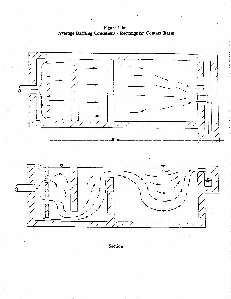
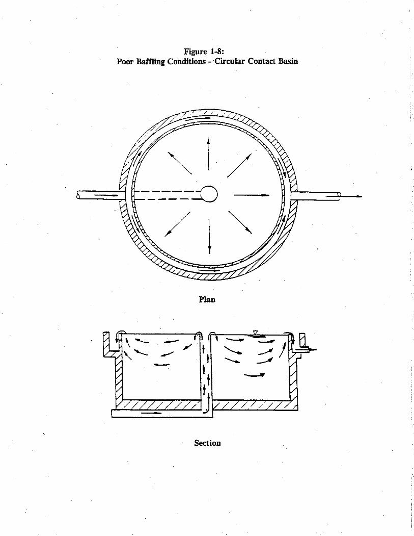
The inlet flow distribution is markedly improved by the addition of an inlet diffuser wall and intra-basin baffling as shown on Figure 1-6. However, only average baffling conditions are achieved for the basin as a whole because of the inadequate outlet structure, a Cipolleti weir. The width of the weir is short in comparison with the width of the basin. Consequently, dead space exists in the corners of the basin, as shown by the plan view. In addition, the small weir width causes a high weir overflow rate, which results in short-circuiting in the center of the basin. Superior baffling conditions are exemplified by the flow pattern and physical characteristics of the basin shown on Figure 1-7. The inlet to the basin consists of submerged, target-baffled ports. This inlet design serves to reduce the velocity of the incoming water and distribute it uniformly throughout the basin's cross-section. The outlet structure is a sharpcrested weir which extends for the entire width of the contact basin. This type of outlet structure will reduce short-circuiting and decrease the dead space fraction of the basin, although the overflow weir does create some dead space at the lower corners of the effluent end. These inlet and outlet structures are by themselves sufficient to attain superior baffling conditions. However, maze-type intra-basin baffling was also included as an example of how this type of baffling aids in flow redistribution within a contact basin. Circular Basins The plan and section of a circular basin with poor baffling conditions, which can be attributed to flow short-circuiting from the center feed well directly to the effluent trough, is shown on Figure 1-8. Short-circuiting occurs in spite of the outlet weir configuration because the center feed inlet is not baffled. The inlet flow distribution is improved somewhat on Figure 1-9 by the addition of an annular ring baffle at the inlet which causes the inlet flow to be distributed throughout a greater portion of the basin's available volume. However, the baffling conditions in this contact basin are only average, because the inlet center feed arrangement does not entirely prevent short-circuiting through the upper levels of the basin. Superior baffling conditions are attained in the basin configuration shown on Figure 1-10 through the addition of a perforated inlet baffle and submerged orifice outlet ports. As indicated by the flow pattern, more of the basin's volume is utilized due to uniform flow distribution created by the perforated baffle. Short-circuiting is also minimized because only a small portion of flow passes directly through the perforated baffle wall from the inlet to the outlet ports.

40

1.3.4 Additional Considerations for Use of Empirical Methods Flocculation basins and ozone contactors represent water treatment processes with slightly different characteristics from those presented in Figures 1-5 through 1-10 because of the additional effects of mechanical agitation and mixing from ozone addition, respectively. Studies by Hudson (1975) indicated that a single-compartment flocculator had a T10/T value less than 0.3, corresponding to a dead space zone of about 20 percent and a very high mixed flow zone of greater than 90 percent. In this study, two four-compartment flocculators, one with and the other without mechanical agitation, exhibited T10/T values in the range of 0.5 to 0.7. This observation indicates that not only will compartmentation result in higher T10/T values through better flow distribution, but also that the effects of agitation intensity on T10/T are reduced where sufficient baffling exists. Therefore, regardless of the extent of agitation, baffled flocculation basins with two or more compartments should be considered to possess average baffling conditions (T10/T = 0.5) whereas unbaffled, single-compartment flocculation basins are characteristic of poor baffling conditions (T10/T = 0.3). Similarly, multiple stage ozone contactors are baffled contact basins which show characteristics of average baffling conditions. Single stage ozone contactors should be considered as being poorly baffled. However, circular, turbine ozone contactors may exhibit flow distribution characteristics which approach those of completely mixed basins, with a T10/T of 0.1, as a result of the intense mixing. In many cases, settling basins are directly connected to the flocculators. Data from Hudson (1975) indicates that poor baffling conditions at the flocculator/settling basin interface can result in backmixing from the settling basin to the flocculator. Therefore, settling basins that have integrated flocculators without effective inlet baffling should be considered as poorly baffled, with a T10/T of 0.3, regardless of the outlet conditions, unless intra-basin baffling is employed to redistribute flow. If intra-basin and outlet baffling is utilized, then the baffling conditions should be considered average with a T10/T of 0.5. Filters are special treatment units because their design and function is dependent on flow distribution that is completely uniform. Except for a small portion of flow which short-circuits the filter media by channeling along the walls of the filter, filter media baffling provides a high percentage of flow uniformity and can be considered superior baffling conditions for the purpose of determining T10. A filter's T10 value can be calculated as follows. Subtract the volume of the filter media, support gravel, and underdrains from the total volume of the filter to obtain the volume available for flow; then calculate the theoretical detention time, T, by dividing this volume by the flow through the filter. The theoretical detention time, T, is then multiplied by a factor of 0.7 (corresponding to superior baffling conditions) to determine T10.

41

1.3.5 Conclusions Regarding the Use of Empirical Methods The recommended T10/T values and examples are presented as a guideline for use by public water systems and their consultants in determining T10 values when tracer studies cannot be performed because of practical considerations. Water systems should refer specifically to WAC 246-290-636(6) for requirements related to use of empirical methods in lieu of tracer studies. Selection of T10/T values in the absence of tracer studies was restricted in this chapter to a qualitative assessment based on currently available data for the relationship between basin baffling conditions and their associated T10/T values. Conditions which are combinations or variations of the above examples may exist and warrant the use of intermediate T10/T values such as 0.4 or 0.6. As more data on tracer studies become available, specifically correlations between other physical characteristics of basins and the flow distribution efficiency parameters, further refinements to the T10/T fractions and definitions of baffling conditions may be appropriate.

42

Chapter 2: Treatment Plant Operations The purpose of this chapter is to provide general guidance to purveyors and their consultants regarding development of treatment plant operations plans. General and technology-specific operating criteria are also included. 2.1 Regulatory Background WAC 246-290-654 addresses minimum filter plant operating criteria and requires purveyors to develop plant-specific operations plans. The regulations specify maximum filtration rates, methods for demonstrating filtration effectiveness and outline some of the basic elements that are to be provided in each operations plan. In addition, the regulations specify that operations plans must be consistent with DOH guidelines for operations procedures. 2.2 Operations Plan The intent of a treatment plant operations plan is to describe tasks an operator needs to perform on a daily basis to remain in compliance with the SWTR as well as to describe emergency operations procedures. The plan should address water quality monitoring, flow measurement and adjustments, chemical dosage procedures and adjustments, CT measurements, monitoring equipment calibration and maintenance, etc. The following outline may be used to guide development of an operations plan for a specific treatment plant:

1. Staffing Provide the name, certification level and certificate number, and phone numbers (home and work) of all plant operations personnel.

2. Monitoring A. Identify the type, frequency, and location of monitoring for all parameters of concern.

At a minimum, this should include: 1. Raw water parameters; 2. Chemical dosages, etc.; 3. Turbidity at individual filters, and combined effluent at entrance to clearwell; and 4. CT monitoring including:

a. Determination of peak hourly flow; b. Disinfectant residual; c. pH; and d. Temperature.

B. Describe laboratory procedures used.

43

C. Describe calibration procedures for all monitoring equipment.

D. Provide a summary of continuous monitoring/recording equipment available at the plant and methods used to assure accuracy of readings.

3. Disinfection A. Determining CT's. The plan should describe how to calculate contact time, and how

to determine and report CT's and the inactivation ratio for Giardia cysts and viruses.

B. Identify system safeguards (automatic switchover, alarms, redundancy, etc.) available to ensure continuous disinfection.

C. Outline the emergency plan to be implemented in case of disinfection failure.

4. Treatment chemicals (e.g. alum, chlorine, polymers, etc.) A. Identify the chemicals used at the plant and their respective chemical suppliers

(including phone numbers).

B. Address the following elements: 1. Safe handling of hazardous materials in the plant; 2. Preparation of feed solutions; 3. Points of application and concentrations of all chemicals fed on a regular basis; 4. Methods for determining appropriate chemical dosages including, at a minimum,

jar test procedures for coagulation facilities; 5. Procedures for adjustment of chemical dosages as water quality changes; 6. Methods of accurately calibrating chemical feed pumps and monitoring chemical

feed rates; and 7. Additional chemical feed capability (e.g. for seasonal application of polymers,

etc.).

5. Filter operation A. Filter backwash procedures, frequency of backwash, and filter run length criteria (i.e.

when and how to initiate backwash - switch, clock timer, etc).

B. Filter-to-waste procedures, and length criteria.

C. Filter scraping procedures and frequency for slow sand filters.

D. Frequency and procedures for filter media inspection and replacement.

E. Pressure filter inspection procedures and records (per WAC 246-290-654).

44

6. Plant control A. Provide a process flow diagram showing location of pumps, valves, and other plant

appurtenances and including all points of chemical injection.

B. Identify flow variations expected and hours the plant is operated. This should include the proposed maximum flow through the plant and address the maximum filtration rates.

C. Describe plant start-up procedures.

D. Describe plant shut-down procedures.

E. Describe the provisions and procedures for manual override of automatic controls including plant operations during computer failures.

F. Describe alarms, remote dialers and automatic shutdown capabilities.

G. Describe plant response to power failures and procedures to be implemented during power failures.

7. Records A. Describe the type and location of records kept at the plant.

B. Records should include, but not be limited to, those necessary for documenting:

1. Monthly compliance with SWTR; 2. Historical information related to coagulants, disinfectants and dosages for varying

source water quality conditions; 3. Calibration of instruments; 4. Weekly verification of turbidimeters; 5. Consumer complaints including waterborne disease outbreaks; 6. Watershed emergencies and the utility's response; and 7. Preventative maintenance.

8. Preventative maintenance program

A. Identify the type and frequency of preventative maintenance conducted at the plant.

B. Identify the type and location of the maintenance records, if not addressed under

Records.

45

9. Emergency response plan A. Identify the procedures to be implemented in case of an emergency including non-

compliance reporting and corrective actions.

B. Include procedures for at least the following types of events: 1. Watershed emergencies (e.g. slides, spills, fires); 2. Treatment failures; and 3. Waterborne disease outbreak.

2.3 Filter Plant Operations Procedures The purpose of the following sections is to provide guidance on treatment plant operations to ensure that the SWTR performance and operations criteria in Part 6 of WAC 246-290 are met. The design and operating criteria for the various filtration technologies found in the latest edition of Recommended Standards for Water Works (Great Lakes, 1992) are the minimum criteria that a majority of states, including Washington, are currently following.1

These standards are referred to as Ten States Standards in the remainder of this document. The criteria contained in Ten States Standards have not been duplicated here.

Rather, the reader is referred to the Ten States Standards directly for design and operating criteria and the DOH Drinking Water Program Water Works Standards for design criteria. DOH does recommend additions and/or changes (described below) to the Ten State Standards to assure compliance with the SWTR performance criteria.

1 Based upon the results of a survey conducted for the American Water Works Association Research Foundation (AWWARF), some 38 states use the Ten States Standards entirely or in modified form (AWWARF, 1986).

46

2.3.1 General for Conventional, Direction and In-line Filter Plants The following recommendations apply to all conventional, direct and in-line filtration plants:

1. All filtration plants should provide continuous turbidity monitoring of the effluent turbidity from each individual filter.2,3

2. All filtration systems should be concerned with the peak turbidity levels in the filtered water after backwashing and should modify operation of the filters to minimize the magnitude and duration of these turbidity spikes.

DOH is planning to recommend this requirement to the State Board of Health for incorporation into the drinking water regulations. If continuous monitoring is impractical for technical reasons, routine monitoring of individual filters is recommended as a minimum.

4

Individual filters should be monitored as discussed above and when excessive turbidity spikes are found, corrective actions should be taken. During these turbidity peaks, Giardia cysts and other pathogens may be passed into the finished water. For example, there is evidence that a 0.2 to 0.3 NTU increase in the turbidity during the first period of the filter run can be associated with rises in Giardia cyst concentrations by factors of twenty to forty (Logsdon, 1985). Special studies should be conducted to determine the extent of the turbidity spike problems. There are basically four approaches available for controlling problems with turbidity spikes after backwashing. These are as follows (Bucklin, et al., 1988):

1. Proper chemical conditioning of the influent water to the filter can minimize the magnitude and duration of these turbidity spikes. This could include proper control of the primary coagulant chemicals such as alum or iron compounds. In many cases, filter aid polymers may be needed to control the turbidity spikes.

2 Although this is not a requirement of the SWTR, it is recommended because of the possibility that not all filters in a treatment plant will produce the same effluent turbidity. This may be due to a variety of conditions that include bed upsets, failure of media support or underdrain systems, etc. Although the combined effluent from all the filters may meet the turbidity requirements of the SWTR, the turbidity level from an individual filter may substantially exceed the limits. This may result in the passage of Giardia cysts or other pathogens. 3 Continuous turbidity measurements shall be validated for accuracy based on the following procedure: turbidity equipment shall be calibrated based upon a primary standard in the expected range of measurements and continuous turbidimeter performance shall be verified on a weekly basis, not on consecutive days, with grab sample measurements being made using a properly calibrated bench model turbidimeter. Validation should be performed at least twice a week based on the procedure outlined in Part 214A in the 16th Edition of Standard Methods. It should be noted that improper installation of continuous monitors may allow for air bubbles to enter the monitor resulting in false turbidity spikes. To avoid air bubbles reaching the turbidimeter the sample tap should be installed below the center line of the pipe and an air release/trap device may be included on the sample line. 4 For most high rate granular bed filters, there is a period of conditioning, or break-in immediately following backwashing, during which turbidity and particle removal is at a minimum, referred to as the break-in period. The turbidity peaks are thought to be caused by remnants of backwash water within the pores of and above the media passing through the filter, and/or floc breakup during the filter ripening period before it can adequately remove influent turbidity.

47

2. Gradually increasing the filtration rate in increments when placing the filter in operation. Starting the filter at a low flow rate and then increasing the flow in small increments over 10 to 15 minutes has been shown to reduce the turbidity spikes in some cases (Logsdon, 1987).

3. Addition of coagulants to the backwash water has also been shown to reduce the extent of turbidity spikes after backwash. Typically, the same primary coagulant used in the plant is added to the backwash water. Polymers alone or in combination with the primary coagulant may also be used.

4. Filter-to-waste may be practiced where a portion of the filtered water immediately after starting the filter is wasted. This is only possible where the filter system has the necessary valves and piping to allow this procedure. Some knowledge of the time actually needed for filter-to-waste is also required before it can be determined that this is an effective procedure for controlling turbidity spikes. If the length of time the filter-to-waste is practiced is less than that before the turbidity spike passes, the disruption caused by the valve operation may actually increase the turbidity spike.

Different treatment plants and the individual filters within the plants may have different turbidity spike characteristics. The four approaches presented above, therefore, must be evaluated on a case-by-case basis. Special studies will be required to identify those filters with the turbidity spike problems and assist in selecting which of the four approaches will best minimize the problem. Turbidity spikes can generally be minimized through one or a combination of the first three approaches. In order to establish filter-to-waste operating guidelines, the following procedure is suggested:

1. Review the effluent turbidity data and/or particle counting data for each filter and determine which filter has historically had the poorest performance (highest effluent turbidity and/or particle counts).

2. Following backwashing of the filter with the poorest performance, place that filter into service and monitor turbidity continuously (or collect grab samples at least every 5 minutes) for a period of at least 60 minutes. Note: particle counting may also be used for this purpose.

3. Analyze the data collected and determine how long the filter must be in operation to achieve the level consistent with ripened filter performance (0.5 NTU filtered water turbidity and/or 80% turbidity reduction across the treatment train).

Limited information exists on the typical magnitude and duration of peak turbidity levels after backwashing and what levels are considered acceptable to assure that these turbidity spikes are not associated with passage of Giardia cysts. Information from plant scale tests showing the typical magnitude and duration of these turbidity spikes is available (Bucklin, et al., 1988). From

48

the studies conducted, the turbidity peaks occurred within the first few minutes after the filter was placed back in operation, their effects lasted for several hours, and they varied in magnitude from 0.08 to 0.35 NTU on average. For existing plants without provisions for filter-to-waste, the decision to add the necessary piping to provide this capability should be made only after carefully evaluating the other three approaches. If the results of special studies show that the other three options are not effective in minimizing the turbidity spikes, then the expense of adding the filter-to-waste capabilities may be justified. For new plants, the capability of filter-to-waste is required by DOH (per WAC 246-290-676). By having this capability, additional flexibility will be available for turbidity spike control. This flexibility may also be useful for other filter maintenance functions such as after media replacement or when heavy chlorination of the filter is needed after maintenance. 2.3.2 Conventional Treatment Conventional treatment is the most widely used technology for removing turbidity and microbial contaminants from surface water supplies. Conventional treatment includes the pretreatment steps of chemical coagulation, rapid mixing, flocculation and sedimentation followed by filtration. Conventional treatment plants typically use aluminum or iron compounds and/or polymers in the coagulation process. Conventional plants may vary in the types of filter media used. Sand filters, normally found in older plants, use a single media of sand to form a filter bed and are generally designed with a filtration rate of 2 gpm/ft2. Newer plants normally use dual-media or mixed media filters. Dual media filters use a combination of anthracite coal along with a sand to form the filter bed. Mixed media filters use coal, sand, and a third material such as fine garnet sand to form the filter bed. Dual and mixed media filters can be designed to operate at higher filtration rates (4 to 6 gpm/ft2) than sand filters. Operating Requirements In addition to the operating requirements in the Ten State Standards, WAC 254-290-654 requires that a coagulant be used at all times the conventional treatment plant is in operation.5 Conventional (direct and in-line filtration plants) must be monitored carefully, because failure to maintain optimum coagulation can result in poor filter performance and breakthrough of cysts and viruses.6

5 Dependable removal of Giardia cysts can not be guaranteed if a water is filtered without being properly coagulated (Logsdon, 1987b; Al-Ani, et al., 1985). This is true even if the raw water turbidity is less than 1 NTU. 6 As indicated in the preamble to the proposed SWTR, 33 percent of the reported cases of giardiasis in waterborne disease outbreaks were attributed to improperly operated filtration plants

49

Although the detention time provided by the settling basins in a conventional plant results in some margin of safety, the loss of coagulation control at the chemical feed or rapid mix points may not be noticed until the poorly coagulated water reaches the filters, after the process has failed. Failure to effectively monitor and control filter operation can result in undetected poor filter performance (Logsdon, 1987a; Logsdon, 1987b). Effective operation of a conventional treatment plant requires careful monitoring and control of chemical feed, rapid mix, flocculation, sedimentation and filtration. For the purposes of the SWTR, the requirements for effective operation of a conventional water treatment plant can be summarized as follows:

1. The application of a coagulant and the maintenance of effective coagulation and flocculation at all times when a treatment plant is in operation.7

a. At least an 80% reduction in source turbidity based on an average of the daily turbidity reduction measured in a calendar month; or

Proper process control procedures should be used at the plant to assure that chemical feeds are adjusted and maintained in response to variations in raw water such as temperature, turbidity, total organic carbon (TOC), color, etc. Per WAC 254-290-654, the effectiveness of coagulation and flocculation shall be demonstrated by one of three methods: turbidity reduction, particle counting, or microscopic particulate analysis. Most systems use the turbidity reduction method. Where raw water turbidity is >2.5 NTU, treatment effectiveness is demonstrated by meeting the turbidity performance standards in WAC 246-290-660. Where raw water turbidity is <2.5 NTU, systems must demonstrate treatment effectiveness by either achieving:

b. A filtered water turbidity <0.10 NTU (based on monthly average).

Systems with source turbidity <2.5 NTU interested in demonstrating treatment effectiveness through a means other than turbidity reduction should contact DOH for guidance.

2. Maintenance of effective filtration will require proper operation procedures to meet the turbidity requirements of the SWTR. Proper operation should include: a. Proper chemical conditioning of the water ahead of the filter to assure adequate

turbidity removal through the filter. The determination of proper chemical control can be made through use of streaming current meters, zeta potential meters, pilot filters, and jar testing. At least one of these process control tools should be used regularly during operation of the treatment plant.

7 Some conventional water treatment plants which treat low turbidity source waters (<1 NTU) reportedly discontinue the application of coagulant(s) during periods of low turbidity since the raw water already meets the turbidity performance standards. However, studies have shown that cyst removal for low turbidity waters is the most difficult to achieve and requires optimum pretreatment including coagulation to achieve effective removals (Al-Ani, et al., 1985).

50

b. Control of the flow rates and elimination of rapid changes in flow rate applied to the filter. Per WAC 254-290-654, conventional gravity filtration plants shall be operated at flow rates not to exceed 3 gpm/ft2 for single media filters and 6 gpm/ft2 for deep bed, dual or mixed media filters.

c. Backwashing of filters before a consistent increase is noted in turbidity and/or particle counts. The criteria on which to base initiation of backwash will have to be determined for each plant. Experience with operation cycles including run times and headloss data may serve as the basis for this site-specific criteria.

d. Bringing the clean filters back on-line after backwash so that turbidity spikes are minimized in the filtered water. Section 2.3.1 discusses these turbidity spikes and approaches available to minimize them.

3. Filters removed from service generally should be backwashed prior to start-up. However, in extreme cases, where it is impractical to backwash filters each time they are removed from service, DOH may allow, on a case-by-case basis, startup without backwashing. In making this decision, the following may be considered: a. The length of time the filter was off-line;

b. Provisions for minimizing the impact of this practice, e.g. ramping valves, use of

filter aids, filter-to waste; and

c. Performance of the filter while being put on-line.

2.3.3 Direct and In-line Filtration A direct filtration plant can include several different pretreatment unit processes depending upon the application. In its simplest form, the process includes only in-line filters preceded by chemical coagulant application and mixing. The mixing step can rarely be satisfied by influent pipeline turbulence, but more typically utilizes in-line or static mixers. In larger filtration plants, an open rapid-mix basin with mechanical mixers is usually employed. Under DOH definitions, the direct filtration process consists of the addition of a coagulant to the raw water followed by rapid mixing and flocculation. The chemically conditioned and flocculated water is then applied directly to a dual-or multi-media filter (USEPA, 1988b). Operating Requirements Operating considerations for in-line and direct filtration plants are essentially identical to those for conventional treatment plants.8

8 Per WAC 254-290-654, pressure filters shall be operated at filtration rates not to exceed 2 gpm/ft2 for single media filters and 3 gpm/ft2 for deep bed, dual or mixed media filters.

The major difference is that direct and in-line filtration plants

51

will not have sedimentation basins, and in-line plants will not have a flocculation or contact basin. All direct filtration plants should make provisions to minimize the impacts of break-in after a filter is put on-line.9

As with conventional treatment, a coagulant must be used at all times when the treatment plant is in operation (WAC 246-290-654).10

Also, like conventional treatment, the initiation of backwashing a filter should first be based on filter effluent turbidity values and/or particle counts, then by headloss and run time. Filters should be backwashed before a consistent increase is noted in filtered water turbidity and/or particle counts.

Also, in general, any filters removed from service should be backwashed prior to start-up. However, in extreme cases, where it is impractical to backwash filters each time they are removed from service, DOH may allow, on a case-by-case basis, startup without backwashing. In making this decision, the DOH will use the same criteria discussed in Section 2.3.2 for conventional plants. Note regarding pressure filters: A pressure filter is similar in principle to the rapid sand gravity filter except that it is completely enclosed in a vertical or horizontal cylindrical steel tank through which water under pressure is filtered. Pressure filters are most frequently used in swimming pool and industrial plant (process water) installations. The main advantage of the pressure filter is that it is possible to use only one pump to take water from the source, force it through the filter and directly into the distribution system. This advantage is offset by the difficulty in introducing chemicals under significant pressure, inadequate coagulation facilities, and lack of adequate settling. In addition, the appearance of the water being filtered and the condition of the sand cannot be observed and the maximum rate of filtration may be exceeded. Also with pressure filters, it is difficult to look inside the filter for the purpose of evaluating backwash efficacy and problems, determining loss of filter media, accumulation of mudballs, need for cleaning, and/or need for replacement of the filter. Because of these disadvantages and weaknesses, a pressure filter is not considered acceptable for the treatment of surface or other contaminated waters to be used for drinking purposes. In fact, Ten State Standards (Section 4.2.2), referenced in WAC 246-290-200, states the following about rapid rate pressure filters: "The normal use of these filters is for iron and manganese removal. Pressure filters shall not be used in the filtration of surface or other polluted waters or following lime-soda softening."

9 As with conventional treatment, direct filtration produces a relatively poor quality filtered water at the beginning of filter runs and therefore a filter-to-waste period is recommended. In some cases, the addition of a filter aid or bringing filters on-line slowly will be appropriate (Cleasby, et al., 1984). 10 Optimum coagulation is critical for effective turbidity and microbiological removals with direct filtration (Al-Ani, et al., 1985).

52

Because of the potential public health problems associated with use of pressure filters for drinking water purposes, DOH has established some operating criteria for existing pressure filters (in addition to the above general criteria specified for direct and in-line filters). These are summarized below:

1. Purveyors must physically inspect and evaluate their pressure filters at least every 6 months for conditions that might reduce their effectiveness in removing Giardia lamblia cysts. Such conditions include but are not limited to: media depth and condition, mudball formation, gravel mounding, and potential for short-circuiting due to cracks in the filter media.

2. Purveyors must keep written records of the inspections and make them available for DOH review. Records should include: a. The dates the inspections were performed;

b. Name(s) of person(s) conducting the inspection;

c. Results of the inspection; and

d. Any corrective actions taken/needed.

2.3.4 Slow Sand Filtration Slow sand filters differ from single-media rapid-rate filters in a number of important characteristics. In addition to the difference of flow rate, slow sand filters function using biological mechanisms as well as physical-chemical mechanisms, use smaller sand particles, and are not backwashed, but rather are cleaned by removing a small fraction of the surface media. In addition, slow sand filters have much longer run times between cleaning, but require a ripening period at the beginning of each run. Although rapid rate filtration is currently the water treatment technology used most extensively for surface water filtration in the United States, its use has often proved inappropriate for small communities since rapid-rate filtration is a technology that requires skilled operation by trained operators. Slow sand filtration requires very little control by an operator. Consequently, use of this technology may be more appropriate for small systems where source water quality is within the guidelines recommended in Chapter 4, Table 4-2. Slow sand filtration also may be applicable to other source water quality conditions with the addition of pretreatment such as roughing filtration as discussed in Chapter 4, Section 4.2.3.

53

Operating Requirements Maintenance of a slow sand filter involves two periodic tasks:

1. Removal of the top 0.8 to 1.2 inches (2 to 3 cm) of the surface of the sand bed when the headloss exceeds about 3 to 5 feet (1 to 1.5 m);11

2. Replacement of the sand when repeated scrapings have reduced the depth of the sand to approximately one-half of its design depth (Bellamy, et al., 1985).

and

Following scraping, slow sand filters produce poorer quality filtrate at the beginning of a run, and a filter-to-waste or ripening period of one to two days is recommended before use to supply the system. The ripening period is an interval of time immediately after a scraped filter is put back on-line, when the turbidity or particle count results are significantly higher than the corresponding values for the operating filter. During this time, the microorganisms multiply and attain equilibrium in the top surface of the filter known as the schmutzdecke. Filter effluent monitoring should be used to determine when the filter has been adequately ripened. For example, a turbidimeter reading of filtered water turbidity similar to that achieved before scraping (1.0 NTU or less) could be used to initiate the start of the filter run. When repeated scrapings of the sand have reduced the depth of the sand bed to approximately one-half of its design depth, the sand should be replaced. Filter bed depths of less than approximately 18 inches (0.46 m) have been shown to result in poor filter performance (Bellamy, et al., 1985). The replacement procedure should include removal of the remaining sand down to the gravel support, the addition of new sand to one half of the design depth and placement of the sand previously removed on top of the new sand.12

The amount of time for the biological population to mature in a new sand filter (also called curing) and to provide stable and full treatment varies. The World Health Organization (1980) reported that curing requires a few weeks to a few months. Fox, et al., (1983) found that about 30 days were required to bring particle and bacterial counts down to a stable level. All researchers agree that a curing time for a new filter is required before the filter operates at its fullest potential (Bellamy, et al., 1985). Research has shown that total coliform reduction across a slow sand filter is a good indicator of bed maturation. Thus, the absence of total coliforms in the filtered water (prior to disinfection) can be used to indicate that the filter is mature.

11 Removal of this top layer of the schmutzdecke should restore the filter to its operational capacity and initial headloss. 12 This procedure results in clean sand being placed in the bottom half of the filter bed and biologically active sand in the top half reducing the amount of time required for the curing period. It also provides for a complete exchange of sand over time, alleviating potential problems of excessive silt accumulation and clogging of the filter bed (Bellamy, et al., 1985).

54

2.3.5 Diatomaceous Earth Filtration Diatomaceous earth (DE) filtration, also known as precoat or diatomite filtration, is appropriate for direct treatment of surface waters for removal of relatively low levels of turbidity and microorganisms. Diatomite filters consist of a layer of DE about 1/8 inch (3 mm) thick supported on a septum or filter element. The thin precoat layer of DE must be supplemented by a continuous body feed of diatomite which is used to maintain the porosity of the filter cake. If no body feed is added, the particles filtered out will build up on the surface of the filter cake and cause rapid increases in headloss. The problems inherent in maintaining the proper thickness of DE on the septum have restricted the use of diatomite filters for municipal purposes, except under certain favorable raw water quality conditions, i.e., low turbidity and good bacteriological quality. Specific upper limits of raw water quality parameters are not well-defined because diatomaceous earth filtration performance depends on the nature, as well as the concentration, of the raw water particles and the grades of diatomite employed. Logsdon (1987b) reported that filtered water turbidities above 1 NTU and short filter runs were observed for several diatomaceous earth plants having maximum raw water turbidities above 20 NTU. Operating Requirements The minimum operating criteria presented in the Ten State Standards for diatomaceous earth filtration are considered sufficient for the purposes of compliance with the SWTR with the following exceptions:

1. The recommended quantity of precoat is 0.2 pounds per square foot of filter area, and the minimum thickness of the precoat filter cake is 1/8 to 1/5 inch.13

2. Treatment plants are also encouraged to provide a coagulant coating (alum or suitable polymer) of the body feed.

14

Operating requirements specific to DE filters include:

o Preparation of body feed and precoat; o Verification that dosages are proper; o Periodic backwashing and disposal of spent filter cake; o Periodic inspection of the septum(s) for cleanliness or damage; and o Verification that the filter is producing filtered water that meets the turbidity performance

criteria.

13 Studies have shown that a precoat thickness of 0.2 lbs/ft2 (1 kg/m2) was most effective in Giardia cyst removal and that the precoat thickness was more important than the grade size in cyst removal (DeWalle, et al., 1984; Logsdon, et al., 1981; Bellamy, et al., 1984). 14 Although enhancement of the DE is not required for Giardia cyst removal, coagulant coating of the body feed has been found to significantly improve removals of viruses, bacteria and turbidity. (Brown, et al., 1974; Bellamy, et al., 1984).

55

2.3.6 Alternate Technologies The SWTR allows the use of filtration technologies other than those specified above provided that the device meets the criteria specified in WAC 246-290-676. These criteria are discussed in detail in Chapter 4, Section 4.2.2. As noted in Chapter 4, DOH maintains an updated list of alternate filtration technologies meeting the criteria specified in WAC 246-290-676. Public water systems interested in obtaining a copy of the list should contact their DOH Regional Office and request the latest DOH Drinking Water Program Alternate Filtration Technology Status Report. Operating Requirements After any necessary pilot studies are conducted and a successful demonstration of performance has been made, operating requirements should follow the manufacturer's recommendations and be approved by DOH through review and approval of the operations plan (to be included with the purveyor's water system plan). Flows and differential pressures must not exceed the maximum values specified in the latest DOH Drinking Water Program Alternate Filtration Technology Status Report. 2.3.7 Additional Information For additional information regarding filter plant operations procedures, water system operators are encouraged to refer to texts, handbooks, and manuals including (but not limited to) those available from the sources listed in Table 2-1.

56

Table 2-1: Water Treatment and Filter Plant Operations Information Sources Information Source / Address General Information Operations Slow Sand Chlorination American Water Works Association (AWWA) 6666 West Quincy Avenue Denver, Colorado 80235

X X X

American Society of Civil Engineers (ASCE) 345 East 47th Street New York, New York 10017

X X

Health Research Inc. Health Education Services Division PO Box 7126 Albany, New York 12224

X X

Ontario Ministry of the Environment Publications available through: Ministry of Government Services Publications Centre 880 Bay Street (5th Floor) Toronto, Ontario M7A 1N8 Canada

X

California State University 600 “J” Street Sacramento, California 95819

X

World Health Organization Publications available through: Q Corporation 49 Sheridan Avenue Albany, New York 12210

X

International Reference Centre PO Box Box 93160 2509 AD The Hague The Netherlands

X

The Chlorine Institute 2001 “L” Street NW Washington, D.C. 20036

X

57

Chapter 3: Procedures for Determining the Level of Inactivation The purpose of this chapter is to outline the procedures for determining the level of inactivation and to provide the CT values needed to make such determinations. 3.1 Regulatory Background WAC 246-290-662 addresses the SWTR disinfection requirements for filtered systems. Under SWTR, disinfection must be provided to ensure that filtration and disinfection together achieve at least a 3-log removal/inactivation of Giardia cysts and a 4-log removal/inactivation of viruses. The required level of inactivation can be achieved by disinfection at any point in the treatment train or distribution system prior to the first customer. Systems must, on a daily basis, determine the level of inactivation achieved, and then determine whether this level is sufficient to meet the required level of inactivation. The required level of inactivation is dependent on the filtration removal credit granted to the system by DOH. The removal credit granted depends on the filtration technology used, and the design, operations and performance of the particular filter plant. Properly designed, well-operated plants using one of the four standard filtration technologies (conventional, direct, slow sand and diatomaceous earth) achieve at least a 2 to 2.5-log removal of Giardia cysts and between a 1 to 2-log removal of viruses. Table 3-1 provides, for the four standard filtration technologies, a summary of the expected levels of Giardia and virus removal (in well-operated plants) and the required minimum levels of disinfection for each technology. When the purveyor believes the treatment processes (excluding disinfection) are achieving greater removals than those listed in Table 3-1, the actual removal provided can be demonstrated through procedures acceptable to DOH. However, when higher removals are demonstrated (i.e.>3-log), systems are still required to provide a minimum of 0.5-log Giardia cyst inactivation and 2-log virus inactivation to supplement filtration and maintain a second treatment barrier for microorganisms.

Table 3-1: Expected Giardia and Virus Removal and Required Log Inactivation

Filtration Expected Log Removals Log Inactivation Required Giardia Viruses Giardia Viruses

Conventional 2.5 2.0 0.5 2.0 Direct, In-line 2.0 1.0 1.0 3.0 Slow Sand 2.0 2.0 1.0 2.0 Diatomaceous Earth 2.0 1.0 1.0 3.0

58

3.2 Procedures for Determining Compliance with the Inactivation Requirements Definitions Disinfectant Residual, C The residual disinfectant concentration, C, is the concentration of the disinfectant in mg/L at a point before or at the first customer. The first customer is considered the first service connection, i.e. the point where water is first withdrawn for human consumption. This definition of first customer pertaining to the point of first consumption assures that the water has received the required disinfection to provide protection from microorganisms for all consumers. The residual disinfectant concentration, C, must be measured daily during peak hourly flow. Peak hourly flow is defined as the greatest volume of water passing through the system during any one hour in a calendar day. Peak hourly flow is not meant to be the absolute peak flow occurring at any instant during the day. Unless a system knows from experience when peak flow will occur, peak hourly flow can only be identified after it has occurred. Therefore, DOH suggests that continuous disinfectant residual monitors be used if a system has variable flow rates. Otherwise a system may take residual measurements every hour. If it is not practical to take grab samples each hour, the system may take grab samples during the period peak flow is expected to occur. The measurements taken during the hour of peak flow can then be used to calculate CT as defined below. Contact Time, T As discussed in Chapter 1, contact time, T, is the time (in minutes) it takes the water, during peak hourly flow, to move between the point of disinfectant application and the point where, C, the residual disinfectant concentration is measured. Guidance for determining contact time in pipelines and contact chambers is provided in Chapter 1. CT Values and Inactivation Ratio A number of disinfectants are available to meet the inactivation requirements. For the various disinfectants, the SWTR prescribes CT values which will achieve different levels of inactivation under various conditions. CT is defined as follows:

CT = C X T where:

C = residual disinfectant concentration in mg/L; and

T = contact time in minutes.

59

The CT values prescribed by SWTR are by definition CTrequired values (CTreq'd) and are provided in the CT tables at the end of this chapter. To determine compliance with the inactivation requirements, a system must calculate the CT value(s) for its disinfection conditions during peak hourly flow each day that the system delivers water to its customers.15

This is by definition the CTcalculated value(s) (CTcalc).

The inactivation ratio for each disinfectant sequence is defined as CTcalc/CTreq'd. If the total inactivation ratio (ΣCTcalc/CTreq'd) is equal to or greater than 1.0, the required level of inactivation has been achieved. In other words, for systems with one disinfection sequence, if the CTcalc is equal to or greater than the CTreq'd, then the system is meeting the disinfection performance requirement. Inactivation Determination Options A system with one point of disinfectant application may determine the level of inactivation based on either of the following methods:

1. One point of residual measurement prior to the first customer; or

2. On a profile of the residual concentration after the point of disinfectant application. Profiling the residual allows for credit of significantly higher residuals which may exist before the water reaches the first customer. However, profiling the residual may not be necessary if one CT is calculated and this CTcalc value exceeds the required CT (CTreq'd) obtained directly from the CT tables. For systems which apply disinfectant at one point and choose not to profile the residual, the following procedure should be used to determine compliance with the inactivation requirements. The total inactivation ratio is calculated as follows:

1. Measure the disinfectant residual, C, at one point within the treatment train prior to the first customer.

2. Determine the contact time, T, between the point of disinfectant application and the point where C is measured.

3. Calculate CT for the point of residual measurement (CTcalc).

15 In contrast to the close control of disinfectant addition and CT monitoring required of unfiltered systems, for filtered systems which have long detention times and regularly exceed the CT requirements for the inactivation level needed, it may be unnecessary to calculate CTs each day of operation. Monitoring the residual at the end of the contact time may be sufficient to indicate that the required level of inactivation is provided.

60

4. Determine CTreq'd by referring to Tables 3-2 through 3-14 using the pH (when chlorine is the disinfectant) and the temperature of the disinfected water at the residual disinfectant concentration sampling point and the required level of Giardia or virus inactivation.16

5. Determine the total inactivation ratio (CTcalc/CTreq'd).

For purposes of determining compliance, if the total inactivation ratio is equal to or greater than 1.0, the system meets the disinfection requirement. For systems which choose to profile the residual from one point of disinfectant application, the residual profile is generated by monitoring the disinfectant residual at several points between the point of disinfectant application and the first customer. The total inactivation achieved is the sum of the inactivation ratios between each of the residual monitoring points. The portion of the system with a measurable contact time between two points of residual monitoring is considered a section. Using this method, the calculated CT (CTcalc) is determined daily for each section. The residual profile and the total inactivation ratio are calculated as follows:

1. Measure the disinfectant residual, C, at any number of points within the treatment train prior to the first customer.

2. Determine the contact time, T, between the point of disinfectant application and the points where C is measured.

3. Calculate CT for each point of residual measurement (CTcalc).

4. Determine CTreq'd for each section by referring to Tables 3-2 through 3-14 using the pH (when chlorine is the disinfectant) and temperatures of the disinfected water for the respective sections (i.e. at each residual measurement point) and the required level of Giardia or virus inactivation.

5. Determine the inactivation ratio (CTcalc/CTreq'd) for each section.

6. Sum the inactivation ratios for each section, i.e., Σ C1T1/CTreq'd + C2T2/CTreq'd + ... + CnTn/CTreq'd, to determine the total inactivation ratio.

For purposes of determining compliance, if the total inactivation ratio is equal to or greater than 1.0, the system meets the disinfection requirement.

16 For systems using chlorine, the CT value for Giardia inactivation will be greater than the CT for viruses and should be the CTreq'd value used. However, for systems using ozone or chloramines, the CT value for virus inactivation may be greater than the CT value for Giardia inactivation. Thus, systems using ozone or chloramines, the controlling CT value is the higher of the two values and should be used for determining compliance.

61

For systems with multiple points of disinfectant application, such as ozone followed by chlorine, or chlorine applied at two different points in the treatment train, the total inactivation is the sum of the inactivation ratios between each of the points of disinfection. In this case, the portion of the system with a measurable contact time between two points of disinfectant application is considered a section. As with the residual profile method, the inactivation ratio of each disinfectant section prior to the first customer may be used to determine the total inactivation ratio. Systems providing disinfection prior to filtration may include the inactivation ratio for the pre-filtration disinfection section when determining the total inactivation ratio. However, calculation of inactivation ratios for each section may not be necessary if one section provides a CTcalc which exceeds the CTreq'd (obtained from the CT tables). To determine the inactivation ratio for each section, the disinfectant residual, C, of each disinfection section and the corresponding contact time, T, must be measured at some point prior to the subsequent disinfection application point(s). Using the same procedure as the residual profile method outlined above, the individual inactivation ratios (CTcalc/CTreq'd) for each of the disinfectant sequences should be added to determine the total inactivation ratio. If the total inactivation ratio is equal to or greater than 1.0, the system meets the disinfection requirement. 3.3 Meeting the Required Inactivation using Various Disinfectants Free Chlorine The effectiveness of free chlorine as a disinfectant is influenced by both the temperature and pH of the water and by the concentration of chlorine. The CT values for the inactivation of Giardia cysts by free chlorine at various temperatures and pHs are presented in Tables 3-2 through 3-7 of this Chapter. The CT values for the inactivation of viruses by free chlorine are presented in Table 3-8. To determine whether a system is meeting the required level of inactivation, the free chlorine residual, pH and temperature must be measured, at the same points prior to the first customer, where contact times, T, are measured. The CTs actually achieved in the system (CTcalc) should then be compared to the CT req'd values in the CT Tables for the pH and temperature of the water at the point(s) of residual measurement. The variation in CT required with respect to the residual for chlorine makes it impractical for systems to continually change the disinfectant dose as the flow changes. Therefore, DOH suggests that the flow variation at the utility be divided into ranges and the residual needed at the higher flow of the range be maintained for all flows within the range to assure adequate disinfection. This approach is outlined in Section 3.4, Example 1.

62

Once the utility has divided the flow into ranges and determined the residuals needed to ensure the required levels of inactivation, maintenance of a residual within the distribution system must also be considered. Although the residuals will meet the required CT, they may or may not be sufficient for maintaining a residual in the distribution system. If there is no other point of disinfection prior to the distribution system, the residual for disinfection must be maintained at a level which will also provide a detectable residual throughout the distribution system. Ozone CT values for the inactivation of Giardia cysts by ozone are presented in Table 3-9 for various temperatures and inactivation rates. As indicated in this table, the CTs required for inactivation with ozone are substantially lower than those required for free chlorine. This reflects the fact that ozone is a more powerful disinfectant. The CT requirements for inactivation of viruses using ozone are presented in Table 3-10. Because of the reactivity of ozone, it is unlikely that a residual will exist for more than a few minutes. As a result, the application of a persistent disinfectant such as chlorine or chloramines is needed to maintain the required disinfectant residual in the distribution system. In lieu of calculating the CT for an ozone contactor or to demonstrate that lower CTs are effective, the disinfection efficiency can be demonstrated through pilot studies acceptable to DOH. Chloramines CT values for the inactivation of Giardia cysts by chloramines are presented in Table 3-11. The high CT values associated with the use of chloramines may be unachievable for some systems. In these cases, chlorine or ozone should be used for primary disinfection, and chloramines for residual disinfection, as necessary. Table 3-12 presents CT values for the inactivation of viruses with chloramines. This table is only applicable for indicating virus inactivation efficiencies if chlorine is added prior to ammonia. Systems which add ammonia prior to chlorine, or ammonia and chlorine concurrently, can determine viral inactivation efficiencies using a protocol acceptable to DOH. Systems may demonstrate effective disinfection with chloramines in lieu of calculating CT or to determine that lower CT values than those indicated in the CT Tables are appropriate. Protocols are available from DOH for these demonstrations. 3.4 Examples for Determined the Level of Inactivation A 20 MGD direct filtration plant applying free chlorine as a disinfectant has a contact time of 27.5 minutes under peak flow conditions. The plant is properly designed and well-operated and has been granted 2-log Giardia cyst removal credit and 1-log virus removal credit by DOH. The plant must provide, through filtration and disinfection, 3-log Giardia removal/inactivation and 4-log virus removal/inactivation.

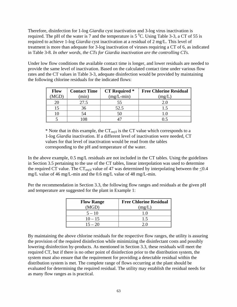
63

Therefore, disinfection for 1-log Giardia cyst inactivation and 3-log virus inactivation is required. The pH of the water is 7 and the temperature is 5 0C. Using Table 3-3, a CT of 55 is required to achieve 1-log Giardia cyst inactivation at a residual of 2 mg/L. This level of treatment is more than adequate for 3-log inactivation of viruses requiring a CT of 6, as indicated in Table 3-8. In other words, the CTs for Giardia inactivation are the controlling CTs. Under low flow conditions the available contact time is longer, and lower residuals are needed to provide the same level of inactivation. Based on the calculated contact time under various flow rates and the CT values in Table 3-3, adequate disinfection would be provided by maintaining the following chlorine residuals for the indicated flows:

Flow (MGD)

Contact Time (min)

CT Required * (mg/L-min)

Free Chlorine Residual (mg/L)

20 27.5 55 2.0 15 36 52.5 1.5 10 54 50 1.0 5 108 47 0.5

* Note that in this example, the CTreq'd is the CT value which corresponds to a 1-log Giardia inactivation. If a different level of inactivation were needed, CT values for that level of inactivation would be read from the tables corresponding to the pH and temperature of the water.

In the above example, 0.5 mg/L residuals are not included in the CT tables. Using the guidelines in Section 3.5 pertaining to the use of the CT tables, linear interpolation was used to determine the required CT value. The CTreq'd value of 47 was determined by interpolating between the <0.4 mg/L value of 46 mg/L-min and the 0.6 mg/L value of 48 mg/L-min. Per the recommendation in Section 3.3, the following flow ranges and residuals at the given pH and temperature are suggested for the plant in Example 1:

Flow Range (MGD)

Free Chlorine Residual (mg/L)

5 – 10 1.0 10 – 15 1.5 15 – 20 2.0

By maintaining the above chlorine residuals for the respective flow ranges, the utility is assuring the provision of the required disinfection while minimizing the disinfectant costs and possibly lowering disinfection by-products. As mentioned in Section 3.3, these residuals will meet the required CT, but if there is no other point of disinfection prior to the distribution system, the system must also ensure that the requirement for providing a detectable residual within the distribution system is met. The complete range of flows occurring at the plant should be evaluated for determining the required residual. The utility may establish the residual needs for as many flow ranges as is practical.

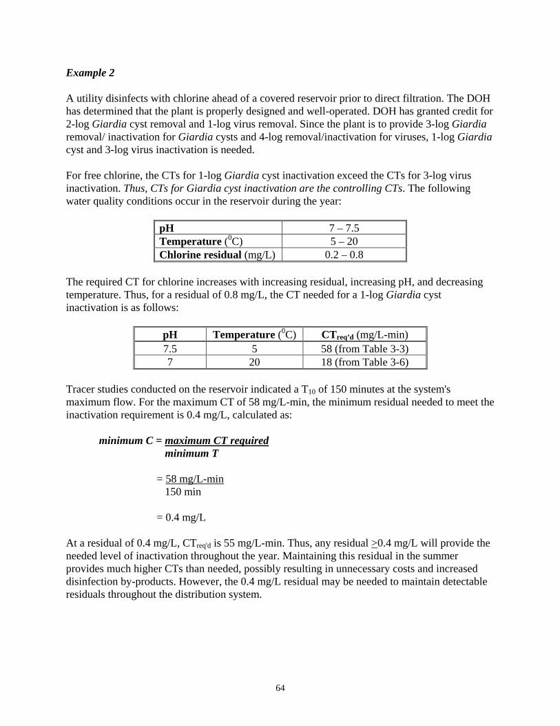
64

Example 2 A utility disinfects with chlorine ahead of a covered reservoir prior to direct filtration. The DOH has determined that the plant is properly designed and well-operated. DOH has granted credit for 2-log Giardia cyst removal and 1-log virus removal. Since the plant is to provide 3-log Giardia removal/ inactivation for Giardia cysts and 4-log removal/inactivation for viruses, 1-log Giardia cyst and 3-log virus inactivation is needed. For free chlorine, the CTs for 1-log Giardia cyst inactivation exceed the CTs for 3-log virus inactivation. Thus, CTs for Giardia cyst inactivation are the controlling CTs. The following water quality conditions occur in the reservoir during the year:

pH 7 – 7.5 Temperature (0C) 5 – 20 Chlorine residual (mg/L) 0.2 – 0.8

The required CT for chlorine increases with increasing residual, increasing pH, and decreasing temperature. Thus, for a residual of 0.8 mg/L, the CT needed for a 1-log Giardia cyst inactivation is as follows:

pH Temperature (0C) CTreq’d (mg/L-min) 7.5 5 58 (from Table 3-3) 7 20 18 (from Table 3-6)

Tracer studies conducted on the reservoir indicated a T10 of 150 minutes at the system's maximum flow. For the maximum CT of 58 mg/L-min, the minimum residual needed to meet the inactivation requirement is 0.4 mg/L, calculated as:

minimum C = maximum CT required minimum T

= 58 mg/L-min

150 min

= 0.4 mg/L At a residual of 0.4 mg/L, CTreq'd is 55 mg/L-min. Thus, any residual >0.4 mg/L will provide the needed level of inactivation throughout the year. Maintaining this residual in the summer provides much higher CTs than needed, possibly resulting in unnecessary costs and increased disinfection by-products. However, the 0.4 mg/L residual may be needed to maintain detectable residuals throughout the distribution system.

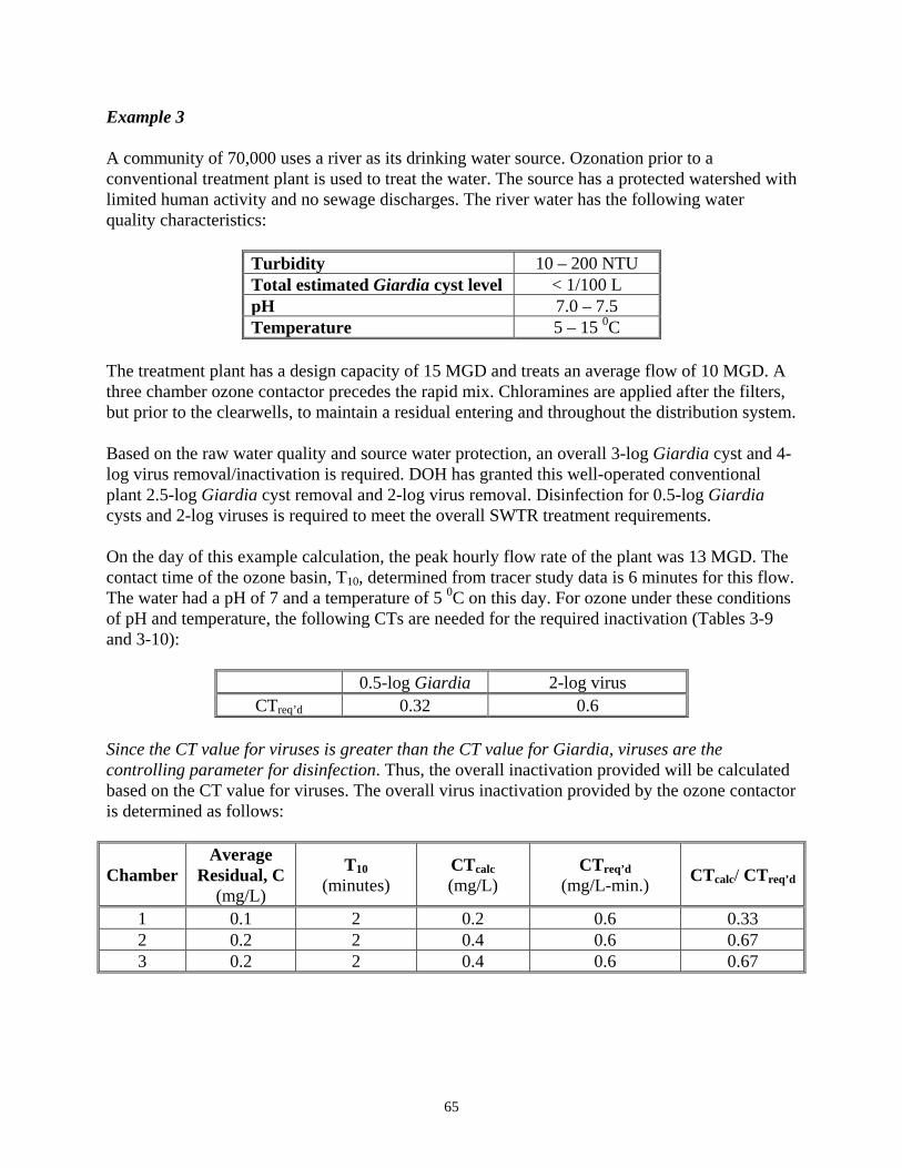
65

Example 3 A community of 70,000 uses a river as its drinking water source. Ozonation prior to a conventional treatment plant is used to treat the water. The source has a protected watershed with limited human activity and no sewage discharges. The river water has the following water quality characteristics:

Turbidity 10 – 200 NTU Total estimated Giardia cyst level < 1/100 L pH 7.0 – 7.5 Temperature 5 – 15 0C

The treatment plant has a design capacity of 15 MGD and treats an average flow of 10 MGD. A three chamber ozone contactor precedes the rapid mix. Chloramines are applied after the filters, but prior to the clearwells, to maintain a residual entering and throughout the distribution system. Based on the raw water quality and source water protection, an overall 3-log Giardia cyst and 4-log virus removal/inactivation is required. DOH has granted this well-operated conventional plant 2.5-log Giardia cyst removal and 2-log virus removal. Disinfection for 0.5-log Giardia cysts and 2-log viruses is required to meet the overall SWTR treatment requirements. On the day of this example calculation, the peak hourly flow rate of the plant was 13 MGD. The contact time of the ozone basin, T10, determined from tracer study data is 6 minutes for this flow. The water had a pH of 7 and a temperature of 5 0C on this day. For ozone under these conditions of pH and temperature, the following CTs are needed for the required inactivation (Tables 3-9 and 3-10):

0.5-log Giardia 2-log virus CTreq’d 0.32 0.6

Since the CT value for viruses is greater than the CT value for Giardia, viruses are the controlling parameter for disinfection. Thus, the overall inactivation provided will be calculated based on the CT value for viruses. The overall virus inactivation provided by the ozone contactor is determined as follows:

Chamber Average

Residual, C (mg/L)

T10 (minutes)

CTcalc (mg/L)

CTreq’d (mg/L-min.) CTcalc/ CTreq’d

1 0.1 2 0.2 0.6 0.33 2 0.2 2 0.4 0.6 0.67 3 0.2 2 0.4 0.6 0.67

66

The total inactivation ratio, i.e. the sum of CTcalc/CTreq'd for the three ozone chambers, is determined as follows:

Total Inactivation Ratio = Σ(C1T1/CTreq'd + C2T2/CTreq'd+ C3T3/CTreq'd)

= Σ(0.33 + 0.67 + 0.67)

= 1.67 Since the total inactivation ratio is greater than 1, the system is in compliance with the required level of inactivation. Example 4 A 2 MGD slow sand filtration plant treating reservoir water, fed by mountain streams with no nearby wastewater discharges, provides drinking water for a community of 8,000 people. The water quality at the intake has the following water quality characteristics:

Turbidity 5 – 10 NTU Total coliforms (100 – 300)/100 ml Total estimated Giardia cyst level < 1/100 L pH 6.5 – 7.5 Temperature 5 – 15 0C

The filtered water turbidity ranges from 0.6 – .8 NTU. DOH has granted this well-operated slow sand plant 2-log Giardia cyst and 2-log virus removal credit. Thus, disinfection for 1-log Giardia cyst and 2-log virus inactivation is required for the system to meet the overall treatment requirements. Chlorine is added prior to the clearwells to provide disinfection. The clearwells have a capacity of 80,000 gallons. A one mile, 16-inch transmission main transports the water from the treatment plant to the first customer. The inactivation provided is determined daily for the peak hourly flow conditions. Tracer studies have been conducted to determine the T10 for the clearwells for different flow rates. For the purposes of calculating the total inactivation achieved, the system is divided into two sections: section 1 - clearwell; and section 2 - transmission main. The flow rate at peak hourly flow from the clearwell was 1.5 MGD on the day of this example. At this flow rate, the T10 of the clearwell is 67 minutes, as determined from the results of the tracer studies. At this flow rate, water travels through the transmission main at 99 ft/min.

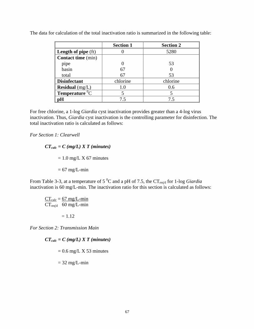
67

The data for calculation of the total inactivation ratio is summarized in the following table:

Section 1 Section 2 Length of pipe (ft) 0 5280 Contact time (min)

pipe 0 53 basin 67 0 total 67 53

Disinfectant chlorine chlorine Residual (mg/L) 1.0 0.6 Temperature 0C 5 5 pH 7.5 7.5

For free chlorine, a 1-log Giardia cyst inactivation provides greater than a 4-log virus inactivation. Thus, Giardia cyst inactivation is the controlling parameter for disinfection. The total inactivation ratio is calculated as follows: For Section 1: Clearwell

CTcalc = C (mg/L) X T (minutes)

= 1.0 mg/L X 67 minutes

= 67 mg/L-min From Table 3-3, at a temperature of 5 0C and a pH of 7.5, the CTreq'd for 1-log Giardia inactivation is 60 mg/L-min. The inactivation ratio for this section is calculated as follows:

CTcalc = 67 mg/L-min CTreq'd 60 mg/L-min

= 1.12

For Section 2: Transmission Main

CTcalc = C (mg/L) X T (minutes)

= 0.6 mg/L X 53 minutes

= 32 mg/L-min

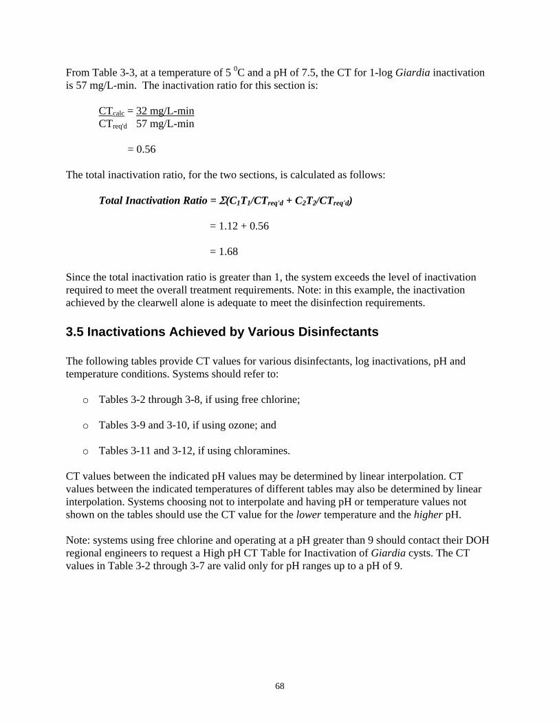
68

From Table 3-3, at a temperature of 5 0C and a pH of 7.5, the CT for 1-log Giardia inactivation is 57 mg/L-min. The inactivation ratio for this section is:

CTcalc = 32 mg/L-min CTreq'd 57 mg/L-min

= 0.56

The total inactivation ratio, for the two sections, is calculated as follows:

Total Inactivation Ratio = Σ(C1T1/CTreq'd + C2T2/CTreq'd)

= 1.12 + 0.56

= 1.68 Since the total inactivation ratio is greater than 1, the system exceeds the level of inactivation required to meet the overall treatment requirements. Note: in this example, the inactivation achieved by the clearwell alone is adequate to meet the disinfection requirements. 3.5 Inactivations Achieved by Various Disinfectants The following tables provide CT values for various disinfectants, log inactivations, pH and temperature conditions. Systems should refer to:

o Tables 3-2 through 3-8, if using free chlorine;

o Tables 3-9 and 3-10, if using ozone; and

o Tables 3-11 and 3-12, if using chloramines. CT values between the indicated pH values may be determined by linear interpolation. CT values between the indicated temperatures of different tables may also be determined by linear interpolation. Systems choosing not to interpolate and having pH or temperature values not shown on the tables should use the CT value for the lower temperature and the higher pH. Note: systems using free chlorine and operating at a pH greater than 9 should contact their DOH regional engineers to request a High pH CT Table for Inactivation of Giardia cysts. The CT values in Table 3-2 through 3-7 are valid only for pH ranges up to a pH of 9.

69

Table 3-2: CT Values for Inactivation of Giardia Cysts by Free Chlorine at 0.5 0C or Lower pH <6 pH = 6.5 pH = 7.0

Chlorine Concentration Log Inactivations Log Inactivations Log Inactivations

(mg/L) <0.4 0.6 0.8 1 1.2 1.4 1.6 1.8 2 2.2 2.4 2.6 2.8 3

0.5

23 24 24 25 25 26 26 27 28 28 29 29 30 30

1.0

46 47 48 49 51 52 52 54 55 56 57 58 59 60

1.5

69 71 73 74 76 78 79 81 83 85 86 88 89 91

2.0

91 94 97 99

101 103 105 108 110 113 115 117 119 121

2.5

114 118 121 123 127 129 131 135 138 141 143 146 148 151

3.0

137 141 145 148 152 155

157162

165 169 172 175 178 181

0.5

27 28 29 29 30 31 32 32 33 34 34 35 36 36

1.0

54 56 57 59 60 61 63 64 66 67 68 70 71 72

1.5

82 84 86 88 90 92 95 97 99

101 103 105 107 109

2.0

109 112 115 117 120 123 126 129 131 134 137 139 142 145

2.5

136 140 143 147 150 153 158 161 164 168 171 174 178 181

3.0

163 168 172 176 180 184 189 193 197 201 205 209 213 217

0.5

33 33 34 35 36 37 38 39 39 40 41 42 43 44

1.0

65 67 68 70 72 74 75 77 79 81 82 84 86 87

1.5

98 100 103 105 108 111 113 116 118 121 124 126 129 131

2.0

130 133 137 140 143 147 151 154 157 161 165 168 171 174

2.5

163 167 171 175 179 184 188 193 197 202 206 210 214 218

3.0

195 200 205 210 215 221 226 231 236 242 247 252 257 261

pH = 7.5 pH = 8.0 pH = 8.5


(mg/L) <=0.4 0.6 0.8 1 1.2 1.4 1.6 1.8 2 2.2 2.4 2.6 2.8 3

0.5

40 40 41 42 43 44 46 47 48 50 50 51 52 53

1.0

79 80 82 84 86 89 91 93 95 99 99

101 103 105

1.5

119 120 123 127 130 133 137 140 143 149 149 152 155 158

2.0

158 159 164 169 173 177 182 186191 198 199 203 207 211

2.5

198 199 205 211 216 222228 233 238 248 248 253 258 263

3.0

237 239 246 253 259 266 273279 286 297 298 304 310 316

0.5

46 48 49 51 52 54 55 56 58 59 60 61 63 64

1.0

92 95 98

101 104 107 110 113 115 118 120 123 125 127

1.5

139 143 148 152 157 161 165 169 173 177 181 184 188 191

2.0

185 191 197 203 209 214 219 225 231 235 241 245 250 255

2.5

231 238 246 253 261 268 274 282 288 294 301 307 313 318

3.0

277 286 295 304 313 321 329 338 346 353 361 368 375 382

0.5

55 57 59 61 63 65 66 68 70 71 73 74 75 77

1.0

110 114 118 122 125 129132 136 139 142 145 148 151 153

1.5

165 171 177 183 188 194 199 204 209 213 218 222 226 230

2.0

219 228 236 243 251 258 265 271 278 284 290 296 301 307

2.5

274 285 295 304 313 323 331 339 348 355 363 370 377 383

3.0

329 342 354 365 376 387 397 407 417 426 435 444 452 460

pH < 9.0

Chlorine Concentration Log Inactivations

(mg/L) <=0.4 0.6 0.8 1 1.2 1.4 1.6 1.8 2 2.2 2.4 2.6 2.8 3

0.5 65 68 70 73 75 77 80 82 83 85 87 89 91 92

1.0 130 136 141 146 150 155 159 163 167 170 174 178 181 184

1.5 195 204 211 219 226 232 239 245 250 256 261 267 272 276

2.0 260 271 281 291 301 309 318 326 333 341 348 355 362 368

2.5 325 339 352 364 376 387 398 408 417 426 435 444 453 460

3.0 390 407 422 437 451 464 477 489 500 511 522 535 543 552

70

Table 3-3: CT Values for Inactivation of Giardia Cysts by Free Chlorine at 5 0C pH <6 pH = 6.5 pH = 7.0


(mg/L) <0.4 0.6 0.8 1 1.2 1.4 1.6 1.8 2 2.2 2.4 2.6 2.8 3

0.5

16 17 17 18 18 18 19 19 19 20 20 20 21 21

1.0

32 33 34 35 36 36 37 38 39 39 40 41 41 42

1.5

49 50 52 53 54 55 56 57 58 59 60 61 62 63

2.0

65 67 69 70 71 73 74 76 77 79 80 81 83 84

2.5

81 83 86 88 89 91 93 95 97 98

100 102 103 105

3.0

97 100 103 105 107 109 111 114 116 118 120 122 124 126

0.5

20 20 20 21 21 22 22 23 23 23 24 24 25 25

1.0

39 40 41 42 42 43 44 45 46 47 48 49 49 50

1.5

59 60 61 63 64 65 66 68 69 70 72 73 74 76

2.0

78 80 81 83 85 87 88 90 92 93 95 97 99

101

2.5

98 100 102 104 106 108 110 113 115 117 119 122 123 126

3.0

117 120 122 125 127 130 132 135 138 140 143 146 148 151

0.5

23 24 24 25 25 26 26 27 28 28 29 29 30 30

1.0

46 48 49 50 51 52 53 54 55 56 57 58 59 61

1.5

70 72 73 75 76 78 79 81 83 85 86 88 89 91

2.0

93 95 97 99

101 103 105 108 110 113 115 117 119 121

2.5

116 119 122 124 127 129 132 135 138 141 143 146 148 152

3.0

139 143 146 149 152 155 158 162 165 169 172 175 178 182

pH = 7.5 pH = 8.0 pH = 8.5


(mg/L) <=0.4 0.6 0.8 1 1.2 1.4 1.6 1.8 2 2.2 2.4 2.6 2.8 3

0.5

28 29 29 30 31 31 32 33 33 34 35 36 36 37

1.0

55 57 58 60 61 62 64 65 67 68 70 71 72 74

1.5

83 86 88 90 92 94 96 98

100 102 105 107 109 111

2.0

111 114 117 119 122 125 128 131 133 136 139 142 145 147

2.5

138 143 146 149 153 156 160 163 167 170 174 178 181 184

3.0

166 171 175 179 183 187 192 196 200 204 209 213 217 221

0.5

33 34 35 36 37 38 39 40 41 41 42 43 44 45

1.0

66 68 70 72 74 76 77 79 81 83 84 86 88 89

1.5

99 102 105 108 111 114 116 119 122 124 127 129 132 134

2.0

132 136 140 144 147 151 155 159 162 165 169 172 175 179

2.5

165 170 175 180 184 189 193 198 203 207 211 215 219 223

3.0

198 204 210 216 221 227 232 238 243 248 253 258 263 268

0.5

39 41 42 43 45 46 47 48 49 50 51 52 53 54

1.0

79 81 84 87 89 91 94 96 98

100 102 104 106 108

1.5

118 122 126 130 134 137 141 144 147 150 153 156 159 162

2.0

157 163 168 173 178 183 187 191 196 200 204 208 212 216

2.5

197 203 210 217 223 228 234 239 245 250 255 260 265 270

3.0

236 244 252 260 267 274 281 287 294 300 306 312 318 324

pH < 9.0


(mg/L) <=0.4 0.6 0.8 1 1.2 1.4 1.6 1.8 2 2.2 2.4 2.6 2.8 3

0.5

47 49 50 52 53 55 56 58 59 60 61 63 64 65

1.0

93 97

100 104 107 110 112 115 118 120 123 125 127 130

1.5

140 146 151 156 160 165 169 173 177 181 184 188 191 195

2.0

186 194 201 208 213 219 225 230 235 241 245 250 255 259

2.5

233 243 251 260

267274

281 288 294 301 307 313 318 324

3.0

279 291 301 312 320 329 337 345 353 361 368 375 382 389

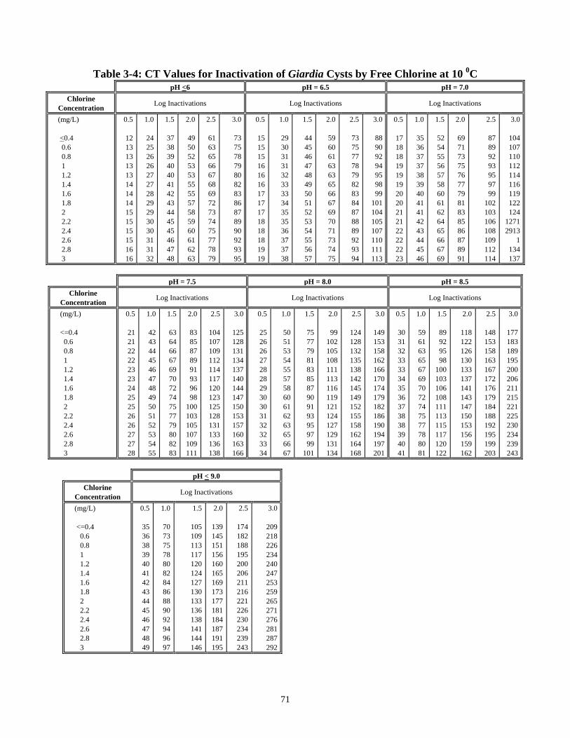
71



(mg/L) <0.4 0.6 0.8 1 1.2 1.4 1.6 1.8 2 2.2 2.4 2.6 2.8 3

0.5

12 13 13 13 13 14 14 14 15 15 15 15 16 16

1.0

24 25 26 26 27 27 28 29 29 30 30 31 31 32

1.5

37 38 39 40 40 41 42 43 44 45 45 46 47 48

2.0

49 50 52 53 53 55 55 57 58 59 60 61 62 63

2.5

61 63 65 66 67 68 69 72 73 74 75 77 78 79

3.0

73 75 78 79 80 82 83 86 87 89 90 92 93 95

0.5

15 15 15 16 16 16 17 17 17 18 18 18 19 19

1.0

29 30 31 31 32 33 33 34 35 35 36 37 37 38

1.5

44 45 46 47 48 49 50 51 52 53 54 55 56 57

2.0

59 60 61 63 63 65 66 67 69 70 71 73 74 75

2.5

73 75 77 78 79 82 83 84 87 88 89 92 93 94

3.0

88 90 92 94 95 98 99

101 104 105 107 110 111 113

0.5

17 18 18 19 19 19 20 20 21 21 22 22 22 23

1.0

35 36 37 37 38 39 40 41 41 42 43 44 45 46

1.5

52 54 55 56 57 58 60 61 62 64 65 66 67 69

2.0

69 71 73 75 76 77 79 81 83 85 86 87 89 91

2.5

87 89 92 93 95 97 99

102 103 106 108 109 112 114

3.0

104 107 110 112 114 116 119 122 124

12712913

1 134 137

pH = 7.5 pH = 8.0 pH = 8.5


(mg/L) <=0.4 0.6 0.8 1 1.2 1.4 1.6 1.8 2 2.2 2.4 2.6 2.8 3

0.5

21 21 22 22 23 23 24 25 25 26 26 27 27 28

1.0

42 43 44 45 46 47 48 49 50 51 52 53 54 55

1.5

63 64 66 67 69 70 72 74 75 77 79 80 82 83

2.0

83 85 87 89 91 93 96 98

100 103 105 107 109 111

2.5

104 107 109 112 114 117 120 123 125 128 131 133 136 138

3.0

125 128 131 134 137 140 144 147 150 153 157 160 163 166

0.5

25 26 26 27 28 28 29 30 30 31 32 32 33 34

1.0

50 51 53 54 55 57 58 60 61 62 63 65 66 67

1.5

75 77 79 81 83 85 87 90 91 93 95 97 99

101

2.0

99 102 105 108 111 113 116 119 121 124 127 129 131 134

2.5

124 128 132 135 138 142 145 149 152 155 158 162 164 168

3.0

149 153 158 162 166 170 174 179 182 186 190 194 197 201

0.5

30 31 32 33 33 34 35 36 37 38 38 39 40 41

1.0

59 61 63 65 67 69 70 72 74 75 77 78 80 81

1.5

89 92 95 98

100 103 106 108 111 113 115 117 120 122

2.0

118 122 126 130 133 137 141 143 147 150 153 156 159 162

2.5

148 153 158 163 167 172 176 179 184 188 192 195 199 203

3.0

177 183 189 195 200 206 211 215 221 225 230 234 239 243

pH < 9.0


(mg/L) <=0.4 0.6 0.8 1 1.2 1.4 1.6 1.8 2 2.2 2.4 2.6 2.8 3

0.5

35 36 38 39 40 41 42 43 44 45 46 47 48 49

1.0

70 73 75 78 80 82 84 86 88 90 92 94 96 97

1.5

105 109 113 117 120 124 127 130 133 136 138 141 144 146

2.0

139 145 151 156 160 165 169 173 177 181 184 187 191 195

2.5

174 182 188 195 200 206 211 216 221 226 230 234 239 243

3.0

209 218 226 234 240 247 253 259 265 271 276 281 287 292

72



(mg/L) <0.4 0.6 0.8 1 1.2 1.4 1.6 1.8 2 2.2 2.4 2.6 2.8 3

0.5

8 8 9 9 9 9 9

10 10 10 10 10 10 11

1.0

16 17 17 18 18 18 19 19 19 20 20 20 21 21

1.5

25 25 26 27 27 28 28 29 29 30 30 31 31 32

2.0

33 33 35 35 36 37 37 38 39 39 40 41 41 42

2.5

41 42 43 44 45 46 47 48 48 49 50 51 52 53

3.0

49 50 52 53 54 55 56 57 58 59 60 61 62 63

0.5

10 10 10 11 11 11 11 11 12 12 12 12 12 13

1.0

20 20 20 21 21 22 22 23 23 23 24 24 25 25

1.5

30 30 31 32 32 33 33 34 35 35 36 37 37 38

2.0

39 40 41 42 43 43 44 45 46 47 48 49 49 51

2.5

49 50 51 53 53 54 55 57 58 58 60 61 62 63

3.0

59 60 61 63 64 65 66 68 69 70 72 73 74 76

0.5

12 12 12 13 13 13 13 14 14 14 14 15 15 15

1.0

23 24 24 25 25 26 26 27 28 28 29 29 30 30

1.5

35 36 37 38 38 39 40 41 42 43 43 44 45 46

2.0

47 48 49 50 51 52 53 54 55 57 57 59 59 61

2.5

58 60 61 63 63 65 66 68 69 71 72 73 74 76

3.0

70 72 73 75 76 78 79 81 83 85 86 88 89 91

pH = 7.5 pH = 8.0 pH = 8.5


(mg/L) <=0.4 0.6 0.8 1 1.2 1.4 1.6 1.8 2 2.2 2.4 2.6 2.8 3

0.5

14 14 15 15 15 16 16 16 17 17 18 18 18 19

1.0

28 29 29 30 31 31 32 33 33 34 35 36 36 37

1.5

42 43 44 45 46 47 48 49 50 51 53 54 55 56

2.0

55 57 59 60 61 63 64 65 67 68 70 71 73 74

2.5

69 72 73 75 77 78 80 82 83 85 88 89 91 93

3.0

83 86 88 90 92 94 96 98

100 102 105 107 109 111

0.5

17 17 18 18 19 19 19 20 20 21 21 22 22 22

1.0

33 34 35 36 37 38 39 40 41 41 42 43 44 45

1.5

50 51 53 54 56 57 58 60 61 62 64 65 66 67

2.0

66 68 70 72 74 76 77 79 81 83 85 86 88 89

2.5

83 85 88 90 93 95 97 99

102 103 106 108 110 112

3.0

99 102 105 108 111 114 116 119 122 124 127 129 132 134

0.5

20 29 21 22 22 23 24 24 25 25 26 26 27 27

1.0

39 41 42 43 45 46 47 48 49 50 51 52 53 54

1.5

59 61 63 65 67 69 71 72 74 75 77 78 80 81

2.0

79 81 84 87 89 91 94 96 98

100 102 104 106 108

2.5

98 102 105

108112

114 118 120 123 125 128 130 133 135

3.0

118 122 126 130 134 137 141 144 147 150 153 156 159 162

pH < 9.0

Chlorine Concentration

Log Inactivations

(mg/L) <=0.4 0.6 0.8 1 1.2 1.4 1.6 1.8 2 2.2 2.4 2.6 2.8 3

0.5

23 24 25 26 27 28 28 29 30 30 31 31 32 33

1.0

47 49 50 52 53 55 56 58 59 60 61 63 64 65

1.5

70 73 76 78 80 83 85 87 89 91 92 94 96 98

2.0

93 97

101 104 107 110 113 115 118 121 123 125 127 130

2.5

117 122 126 130 133 138 141 144 148 151 153 157 159 163

3.0

140 146 151 156 160 165 169 173 177 181 184 188 191 195

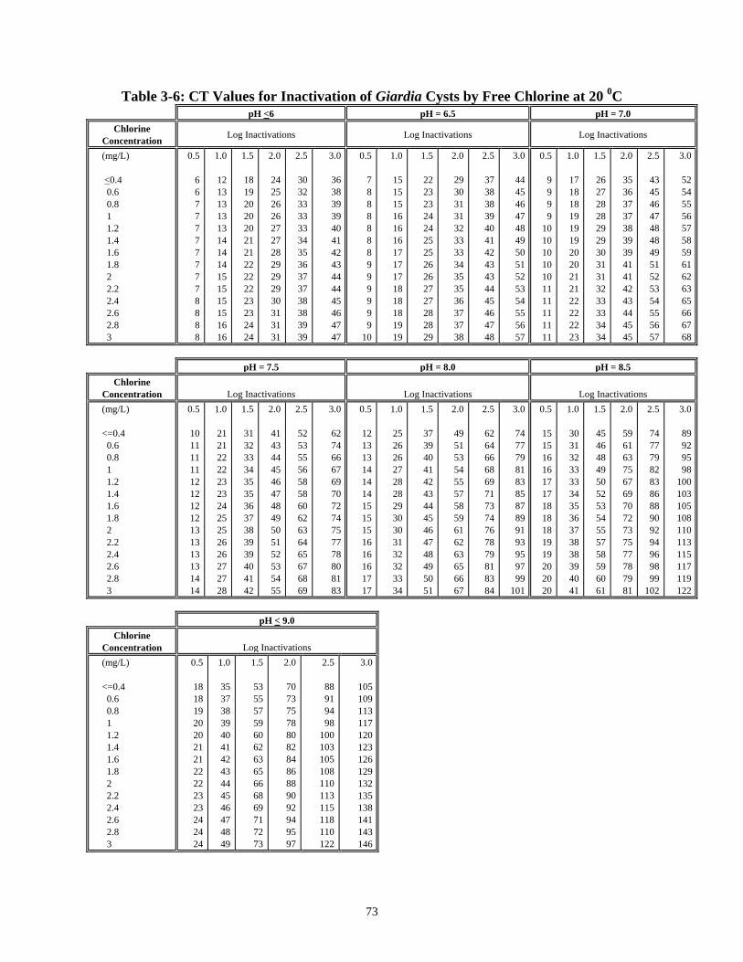
73



(mg/L) <0.4 0.6 0.8 1 1.2 1.4 1.6 1.8 2 2.2 2.4 2.6 2.8 3

0.5

6 6 7 7 7 7 7 7 7 7 8 8 8 8

1.0

12 13 13 13 13 14 14 14 15 15 15 15 16 16

1.5

18 19 20 20 20 21 21 22 22 22 23 23 24 24

2.0

24 25 26 26 27 27 28 29 29 29 30 31 31 31

2.5

30 32 33 33 33 34 35 36 37 37 38 38 39 39

3.0

36 38 39 39 40 41 42 43 44 44 45 46 47 47

0.5

7 8 8 8 8 8 8 9 9 9 9 9 9

10

1.0

15 15 15 16 16 16 17 17 17 18 18 18 19 19

1.5

22 23 23 24 24 25 25 26 26 27 27 28 28 29

2.0

29 30 31 31 32 33 33 34 35 35 36 37 37 38

2.5

37 38 38 39 40 41 42 43 43 44 45 46 47 48

3.0

44 45 46 47 48 49 50 51 52 53 54 55 56 57

0.5

9 9 9 9

10 10 10 10 10 11 11 11 11 11

1.0

17 18 18 19 19 19 20 20 21 21 22 22 22 23

1.5

26 27 28 28 29 29 30 31 31 32 33 33 34 34

2.0

35 36 37 37 38 39 39 41 41 42 43 44 45 45

2.5

43 45 46 47 48 48 49 51 52 53 54 55 56 57

3.0

52 54 55 56 57 58 59 61 62 63 65 66 67 68

pH = 7.5 pH = 8.0 pH = 8.5


Log Inactivations

Log Inactivations

Log Inactivations

(mg/L) <=0.4 0.6 0.8 1 1.2 1.4 1.6 1.8 2 2.2 2.4 2.6 2.8 3

0.5

10 11 11 11 12 12 12 12 13 13 13 13 14 14

1.0

21 21 22 22 23 23 24 25 25 26 26 27 27 28

1.5

31 32 33 34 35 35 36 37 38 39 39 40 41 42

2.0

41 43 44 45 46 47 48 49 50 51 52 53 54 55

2.5

52 53 55 56 58 58 60 62 63 64 65 67 68 69

3.0

62 74 66 67 69 70 72 74 75 77 78 80 81 83

0.5

12 13 13 14 14 14 15 15 15 16 16 16 17 17

1.0

25 26 26 27 28 28 29 30 30 31 32 32 33 34

1.5

37 39 40 41 42 43 44 45 46 47 48 49 50 51

2.0

49 51 53 54 55 57 58 59 61 62 63 65 66 67

2.5

62 64 66 68 69 71 73 74 76 78 79 81 83 84

3.0

74 77 79 81 83 85 87 89 91 93 95 97 99

101

0.5

15 15 16 16 17 17 18 18 18 19 19 20 20 20

1.0

30 31 32 33 33 34 35 36 37 38 38 39 40 41

1.5

45 46 48 49 50 52 53 54 55 57 58 59 60 61

2.0

59 61 63 75 67 69 70 72 73 75 77 78 79 81

2.5

74 77 79 82 83 86 88 90 92 94 96 98 99

102

3.0

89 92 95 98

100 103 105 108 110 113 115 117 119 122

pH < 9.0


Log Inactivations

(mg/L) <=0.4 0.6 0.8 1 1.2 1.4 1.6 1.8 2 2.2 2.4 2.6 2.8 3

0.5

18 18 19 20 20 21 21 22 22 23 23 24 24 24

1.0

35 37 38 39 40 41 42 43 44 45 46 47 48 49

1.5

53 55 57 59 60 62 63 65 66 68 69 71 72 73

2.0

70 73 75 78 80 82 84 86 88 90 92 94 95 97

2.5

88 91 94 98

100 103 105 108 110 113 115 118 110 122

3.0

105 109 113 117 120 123 126 129 132 135 138 141 143 146

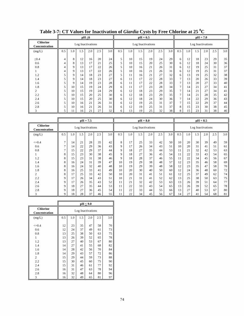
74



(mg/L) <0.4 0.6 0.8 1 1.2 1.4 1.6 1.8 2 2.2 2.4 2.6 2.8 3

0.5

4 4 4 4 5 5 5 5 5 5 5 5 5 5

1.0

8 8 9 9 9 9 9

10 10 10 10 10 10 11

1.5

12 13 13 13 14 14 14 15 15 15 15 16 16 16

2.0

16 17 17 17 18 18 19 19 19 20 20 21 21 21

2.5

20 21 22 22 23 23 23 24 24 25 25 26 26 27

3.0

24 25 26 26 27 27 28 29 29 30 30 31 31 32

0.5

5 5 5 5 5 6 6 6 6 6 6 6 6 6

1.0

10 10 10 10 11 11 11 11 12 12 12 12 12 13

1.5

15 15 16 16 16 17 17 17 18 18 18 19 19 19

2.0

19 20 21 21 21 22 22 23 23 23 24 25 25 25

2.5

24 25 26 26 27 28 28 28 29 29 30 31 31 32

3.0

29 30 31 31 32 33 33 34 35 35 36 37 37 38

0.5

6 6 6 6 6 7 7 7 7 7 7 7 8 8

1.0

12 12 12 12 13 13 13 14 14 14 14 15 15 15

1.5

18 18 19 19 19 20 20 21 21 21 22 22 23 23

2.0

23 24 25 25 25 26 27 27 27 28 29 29 30 31

2.5

29 30 31 31 32 33 33 34 34 35 36 37 38 38

3.0

35 36 37 37 38 39 40 41 41 42 43 44 45 46

pH = 7.5 pH = 8.0 pH = 8.5


(mg/L) <=0.4 0.6 0.8 1 1.2 1.4 1.6 1.8 2 2.2 2.4 2.6 2.8 3

0.5

7 7 7 8 8 8 8 8 8 9 9 9 9 9

1.0

14 14 15 15 15 16 16 16 17 17 17 18 18 18

1.5

21 22 22 23 23 24 24 25 25 26 26 27 27 28

2.0

28 29 29 30 31 31 32 33 33 34 35 35 36 37

2.5

35 36 37 38 38 39 40 41 42 43 43 44 45 46

3.0

42 43 44 45 46 47 48 49 50 51 52 53 54 55

0.5

8 9 9 9 9

10 10 10 10 10 11 11 11 11

1.0

17 17 18 18 18 19 19 20 20 21 21 22 22 22

1.5

25 26 27 27 28 29 29 30 31 31 32 33 33 34

2.0

33 34 35 36 37 38 39 40 41 41 42 43 44 45

2.5

42 43 44 45 46 48 48 50 51 52 53 54 55 56

3.0

50 51 53 54 55 57 58 60 61 62 63 65 66 67

0.5

10 10 11 11 11 12 12 12 12 13 13 13 13 14

1.0

20 20 21 22 22 23 23 24 25 25 26 26 27 27

1.5

30 31 32 33 34 35 35 36 37 38 39 39 40 41

2.0

39 41 42 43 45 46 47 48 49 50 51 52 53 54

2.5

49 51 53 54 56 58 58 60 62 63 64 65 67 68

3.0

59 61 63 65 67 69 70 72 74 75 77 78 80 81

pH < 9.0


(mg/L) <=0.4 0.6 0.8 1 1.2 1.4 1.6 1.8 2 2.2 2.4 2.6 2.8 3

0.5

12 12 13 13 13 14 14 14 15 15 15 16 16 16

1.0

23 24 25 26 27 27 28 29 29 30 31 31 32 32

1.5

35 37 38 39 40 41 42 43 44 45 46 47 48 49

2.0

47 49 50 52 53 55 56 57 59 60 61 63 64 65

2.5

58 61 63 65 67 68 70 72 73 75 77 78 80 81

3.0

70 73 75 78 80 82 84 86 88 90 92 94 96 97

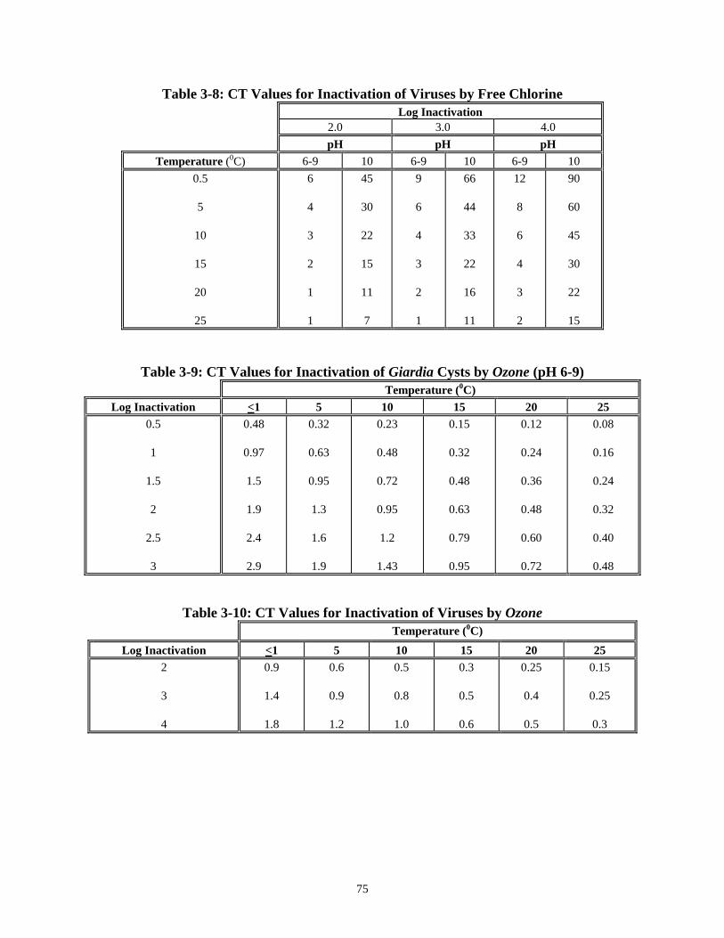
75

Table 3-8: CT Values for Inactivation of Viruses by Free Chlorine Log Inactivation 2.0 3.0 4.0 pH pH pH

Temperature (0C) 6-9 10 6-9 10 6-9 10 0.5

5

10

15

20

25

6

4

3

2

1 1

45

30

22

15

11

7

9

6

4

3

2 1

66

44

33

22

16

11

12

8

6

4

3 2

90

60

45

30

22

15

Table 3-9: CT Values for Inactivation of Giardia Cysts by Ozone (pH 6-9) Temperature (0C)

Log Inactivation <1 5 10 15 20 25 0.5

1

1.5

2

2.5 3

0.48

0.97

1.5

1.9

2.4

2.9

0.32

0.63

0.95

1.3

1.6

1.9

0.23

0.48

0.72

0.95

1.2

1.43

0.15

0.32

0.48

0.63

0.79

0.95

0.12

0.24

0.36

0.48

0.60

0.72

0.08

0.16

0.24

0.32

0.40

0.48

Table 3-10: CT Values for Inactivation of Viruses by Ozone Temperature (0C)

Log Inactivation <1 5 10 15 20 25 2

3

4

0.9

1.4

1.8

0.6

0.9

1.2

0.5

0.8

1.0

0.3

0.5

0.6

0.25

0.4

0.5

0.15

0.25

0.3

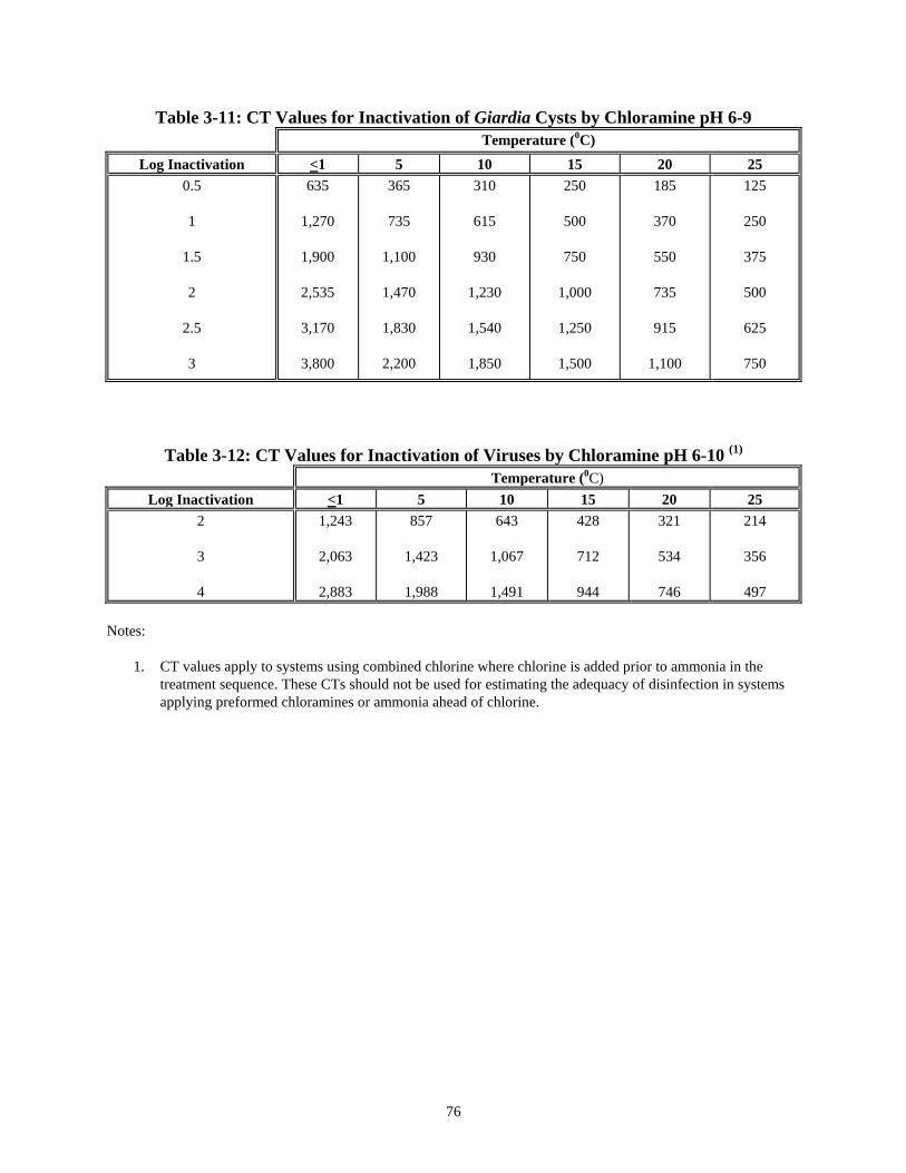
76

Table 3-11: CT Values for Inactivation of Giardia Cysts by Chloramine pH 6-9 Temperature (0C)

Log Inactivation <1 5 10 15 20 25 0.5

1

1.5

2

2.5

3

635

1,270

1,900

2,535

3,170

3,800

365

735

1,100

1,470

1,830

2,200

310

615

930

1,230

1,540

1,850

250

500

750

1,000

1,250

1,500

185

370

550

735

915

1,100

125

250

375

500

625

750

Table 3-12: CT Values for Inactivation of Viruses by Chloramine pH 6-10 (1) Temperature (0C)

Log Inactivation <1 5 10 15 20 25 2

3

4

1,243

2,063

2,883

857

1,423

1,988

643

1,067

1,491

428

712

944

321

534

746

214

356

497

Notes:

1. CT values apply to systems using combined chlorine where chlorine is added prior to ammonia in the treatment sequence. These CTs should not be used for estimating the adequacy of disinfection in systems applying preformed chloramines or ammonia ahead of chlorine.

77

Chapter 4: Criteria for Selection of Filtration Technology 4.1 Regulatory Background To comply with the SWTR, public water systems must include filtration in their treatment processes unless they are able to meet the criteria to remain unfiltered. Per WAC 246-290-676, systems installing filtration must select a filtration technology acceptable to DOH using criteria such as those discussed in this chapter. Once filtration is installed, systems must meet criteria pertaining to design, operation and performance. These criteria are specified in WAC 246-290 as well as Chapter 2 of this Guidance Manual and the DOH Drinking Water Program Waterworks Standards. This section provides general guidance for water systems installing filtration and includes information on the various filtration technologies that may be used to comply with the SWTR. Brief descriptions, removal capabilities, and a listing of major factors to be considered in the selection of a filtration technology, including raw water quality considerations, are provided. In addition, some currently available alternate filtration technologies are described. Finally, alternatives to filtration are briefly discussed. 4.2 Selection of Appropriate Filtration Technology Filtration is generally provided by passing water through a bed of sand, a layer of diatomaceous earth or a combination bed of coarse anthracite coal overlaying finer sand. Filters are classified and named in a number of ways. For example, based on application rate, sand filters can be classified as either slow or rapid; yet, these two types of filters differ in many more characteristics than just application rate. They differ in their removal process, bed material, method of cleaning, and operation. Based on the type of bed material, filters can be classified as sand, diatomaceous earth, dual-media (coal-sand) or even multi-media in which a third layer of high density sand is used. 4.2.1 General Descriptions Current technologies specified by the SWTR are:

1. Conventional Treatment: A series of processes including coagulation, flocculation, sedimentation and rapid rate filtration.

2. Direct and In-line Filtration: A series of processes including coagulation, perhaps flocculation (direct filtration plants only), and rapid rate filtration, but excluding sedimentation.

78

3. Slow Sand Filtration: A process which involves passage of raw water through a bed of sand at low velocity, generally less than 1.2 ft/hr (0.4 meters/hour), resulting in substantial particulate removal by physical and biological mechanisms.

4. Diatomaceous Earth (DE) Filtration: A process meeting the following general conditions: a. A precoat cake of diatomaceous earth filter media is deposited on a support fixture

(septum).

b. The water is filtered by passing it through the cake on the septum; additional filter media, known as body feed, is continuously added to the feed water in order to maintain the permeability of the filter cake.

5. Alternate Technologies: Any filtration process other than the four standard technologies listed above. Alternate technologies are proprietary devices which utilize a straining (or occlusion) media to remove Giardia cysts. With the exception of membrane filters, they generally do not remove viruses. Alternate filtration technologies include, but are not limited to: a. Cartridge Filters;

b. Bag Filters; and

c. Membrane Filters.

4.2.2 Removal Capabilities of Filtration Processes Filtration processes provide various levels of turbidity and microbial contaminant removal. When properly designed and operated and when treating source waters of suitable quality, the above filtration processes are capable of achieving at least a 2-log (99 percent) removal of Giardia cysts and at least a 1-log (90 percent) removal of viruses without disinfection (Logsdon, 1987b; USEPA, 1988b; Roebeck, 1962). The exception is cartridge and bag-type filters which may not provide effective virus removal. Standard Filtration Technologies A summary of the removal capabilities of the four standard filtration processes is presented in Table 4-1.

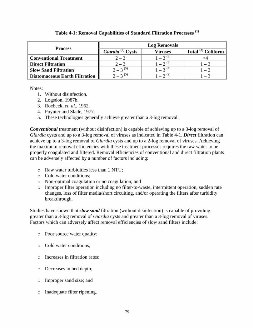
79

Table 4-1: Removal Capabilities of Standard Filtration Processes (1)

Process Log Removals Giardia (2) Cysts Viruses Total (3) Coliform

Conventional Treatment 2 – 3 1 – 3 (3) >4 Direct Filtration 2 – 3 1 – 2 (3) 1 – 3 Slow Sand Filtration 2 – 3 (5) 1 – 3 (4) 1 – 2 Diatomaceous Earth Filtration 2 – 3 (5) 1 – 2 (2) 1 – 3 Notes:

1. Without disinfection. 2. Logsdon, 1987b. 3. Roebeck, et. al., 1962. 4. Poynter and Slade, 1977. 5. These technologies generally achieve greater than a 3-log removal.

Conventional treatment (without disinfection) is capable of achieving up to a 3-log removal of Giardia cysts and up to a 3-log removal of viruses as indicated in Table 4-1. Direct filtration can achieve up to a 3-log removal of Giardia cysts and up to a 2-log removal of viruses. Achieving the maximum removal efficiencies with these treatment processes requires the raw water to be properly coagulated and filtered. Removal efficiencies of conventional and direct filtration plants can be adversely affected by a number of factors including:

o Raw water turbidities less than 1 NTU; o Cold water conditions; o Non-optimal coagulation or no coagulation; and o Improper filter operation including no filter-to-waste, intermittent operation, sudden rate

changes, loss of filter media/short circuiting, and/or operating the filters after turbidity breakthrough.

Studies have shown that slow sand filtration (without disinfection) is capable of providing greater than a 3-log removal of Giardia cysts and greater than a 3-log removal of viruses. Factors which can adversely affect removal efficiencies of slow sand filters include:

o Poor source water quality;

o Cold water conditions;

o Increases in filtration rates;

o Decreases in bed depth;

o Improper sand size; and

o Inadequate filter ripening.

80

Diatomaceous earth (DE) filtration can achieve greater than a 3-log removal of Giardia cysts when sufficient precoat and body feed are used. However, turbidity and total coliform removals are strongly influenced by the grade of DE employed. DE filtration is not very effective for removing viruses, unless the surface properties of the diatomaceous earth have been altered by pretreatment of the body feed with alum or a suitable polymer. In general, DE filtration is assumed to achieve only a 1-log removal of viruses unless demonstrated otherwise. Factors which can affect the removal of Giardia cysts and viruses by DE filtration include:

o Precoat thickness; o Amount of body feed; o Grade of DE; o Improper conditioning of septum; o Loss of filter cake; and o Improper pretreatment of the body feed.

For the purpose of selecting the appropriate filtration and disinfection technologies and for determining design criteria, any of the four standard filtration processes should be assumed to achieve a 2-log removal of Giardia cysts and a 1-log removal of viruses. This conservative approach will assure that the treatment facility has adequate capability to respond to non-optimum performance due to changes in raw water quality, treatment plant upsets, etc. The balance of the required inactivation of Giardia cysts and viruses would be achieved through the application of appropriate disinfection. Alternate Filtration Technologies Although the four standard filtration technologies are effective for removing Giardia lamblia cysts and viruses and are in wide use today, these technologies are often too complex, costly and difficult for small systems to operate properly. Acknowledging these limitations, the SWTR allows alternate filtration devices to be used if the effectiveness of the units can be demonstrated to DOH's satisfaction. Alternate filtration devices include cartridge, bag and membrane filters, which primarily rely on a straining principle to remove most harmful micro-organisms. Cartridge and bag filters using microporous filter elements (ceramic, paper or fiber) with pore sizes as small as 0.2 um may be suitable for producing potable water from raw water supplies containing low levels of turbidity, algae and microbiological contaminants. The advantage to small public water systems of these filters is that, with the exception of disinfectant, no other chemicals are usually required. The process is one of strictly physical removal of small particles by straining as the water passes through a porous medium. Other than occasional cleaning or cartridge replacement, operational requirements for cartridge and bag filtration systems are not complex and do not require skilled personnel. However, the SWTR does require each surface water system to be operated by a certified operator. Cartridge and bag systems may be suitable for some small or seasonally-operated systems where generally only maintenance personnel are available for operating water supply facilities.

81

The application of cartridge and bag filters using either cleanable ceramic or disposable polypropylene cartridges appears to be a feasible method for small systems to remove turbidity and most microbiological contaminants. However, in general, cartridge and bag filters do not remove viruses. Systems using such filters which do not remove viruses will need to meet the overall removal/inactivation requirements by achieving a 4-log inactivation of viruses through disinfection alone. Note: a comparison of Tables 3-2 through 3-7 with Table 3-8 indicates that systems which achieve a 0.5-log inactivation of Giardia cysts, using free chlorine, will achieve greater than a 4-log inactivation of viruses. Consideration should be given to the feasibility of providing multiple barriers of treatment for each target organism, i.e., some Giardia and virus removal by each barrier (i.e., some removal by filtration and some inactivation by disinfection) as protection in case one of the barriers fails. The efficiency and economics of the process must be closely evaluated for each situation. In general, the use of cartridge and bag filters should be limited to relatively low turbidity source waters because of the filter's susceptibility to rapid headloss buildup. For example, manufacturer's guidelines for achieving reasonable filter run lengths with certain polypropylene filter elements are that the raw water turbidity be 2 NTU or less (USEPA, 1988b). As with slow sand filters, pretreatment in the form of roughing filters (rapid sand or multi-media) or fine mesh screens may be used to remove larger suspended solids which, if not removed, could cause the rapid buildup of headloss across the cartridges (USEPA, 1988a). Test results for a number of alternate filtration devices have been evaluated or are currently under evaluation by DOH. Purveyors interested in installing alternate filtration devices may obtain a copy of the current Drinking Water Program Alternate Filtration Technology Status Report by contacting their DOH Regional Office. The Report lists the evaluation status of the alternate filtration devices whose test results have been submitted to DOH for review. Reverse osmosis is a membrane filtration method which is used for desalination and/or the removal of organic contaminants. The treatment process is effective for the removal of Giardia cysts and viruses and no demonstration is necessary. 4.2.3 Factors to Consider When Selecting a Filtration Technology For any specific site and situation, a number of factors will determine which filtration technology is most appropriate. Among these are: raw water quality conditions, operations and maintenance requirements, space and personnel availability, and economic constraints. A discussion of the impact of raw water quality on the technology selection is presented here. The impact of site-specific factors and economic constraints is presented in the USEPA document Technologies and Costs for the Removal of Microbial Contaminants from Potable Water Supplies (USEPA, 1988b).

82

4.2.3.1 Raw Water Quality Conditions General guidelines for selecting filtration processes, based on total coliform count, turbidity, and color are presented in Table 4-2. Filtration systems other than those listed in Table 4-2 should not be used when the general raw water quality conditions exceed the values listed, unless it has been demonstrated through pilot testing that the technology can meet the operations and turbidity performance criteria in Part 6 of WAC 246-290 under the raw water quality conditions expected to occur at the site. When combined with disinfection, the four standard filtration processes are capable of achieving the required 3-log Giardia removal/inactivation and 4-log virus removal/inactivation performance criteria when properly designed and operated, if they are treating a source water of suitable quality, i.e. generally within the ranges indicated in Table 4-2. One of the causes of filtration failures is the use of inappropriate technology for a given raw water quality (Logsdon, 1987b). The criteria in Table 4-2 are considered general guidelines. Periodic occurrences of raw water coliform, turbidity or color levels in excess of the values presented in Table 4-2 should not preclude the selection or use of a particular filtration technology. For example, the following alternatives are available for responding to occasional raw water turbidity spikes:

1. Direct Filtration a. Continuous monitoring and coagulant dose adjustment b. More frequent backwash of filters c. Use of presedimentation

2. Slow Sand Filtration

a. Use of a roughing filter b. Use of an infiltration gallery

3. Diatomaceous Earth (DE) Filtration

a. Use of a roughing filter b. Use of additional body feed

For the above alternatives, pilot testing is required to demonstrate the efficacy of the treatment alternative for a particular site.

83

Table 4-2: Generalized Capability of Filtration Systems to Accommodate Raw Water Quality Conditions

General Restrictions

Treatment Total Coliforms (#/100 ml)

Turbidity (NTU) Color (CU)

Conventional with predisinfection < 20,000 (1) No restrictions (1) <75 (2) Conventional without predisinfection < 5,000 (1) No restrictions (1) < 75 (2) Direct filtration with flocculation < 500 (1) < 7 – 14 (3) < 40 (4) In-line filtration < 500 (1) < 7 – 14 (3) < 10 (1) Slow sand filtration < 800 (5) <10 (5) <5 (1) Diatomaceous earth filtration <50 (1) <5 (1) <5 (1) Notes:

1. Letterman, 1986. 2. USEPA, 1971. 3. Depends on algae population, alum or cationic polymer coagulation (Cleasby, et al.,

1984). 4. Bishop, et al., 1980. 5. Slexak and Sims, 1984. Note: DOH will allow source turbidity levels up to 100 NTUs if

an effective roughing filter is used. 4.2.3.2 Additional Considerations As stated previously, the characteristics of each filtration technology are a major factor in the selection process. Significant characteristics include performance capabilities (contaminant removal efficiencies), design and construction requirements, and operation and maintenance requirements. This chapter has addressed performance capabilities and raw water quality considerations. Details regarding design and construction of the four standard filtration technologies can be found in the most recently published edition of the Ten State Standards, DOH Drinking Water Program Waterworks Standards, and current college texts and professional journal articles. Information regarding operations and maintenance can be found in Ten State Standards, Chapter 2 of this Guidance Manual and texts, handbooks and manuals available from a number of sources including the American Water Works Association, American Society of Civil Engineers, California State University and the Chlorine Institute (see Table 2-1). For small systems required to install filtration, DOH recommends that nontreatment (nonfiltration) options be considered before filtration. Nontreatment alternatives are discussed in Section 4.3. Where nontreatment options are not viable for a system, the criteria for selection of a filtration technology for a small system are essentially the same as those for a larger community.

84

That is, the list of available filtration alternatives should be screened to eliminate those which are either not technically suited to the raw water conditions (Table 4-2) or are not affordable by the utility. Remaining alternatives should then be evaluated based on both costs (capital, annual, and life-cycle) and non-cost factors. Non-cost factors would include operation, maintenance and technical requirements of the filter plant versus the level of operator expertise available and historical reliability of water system from a management, operations and maintenance standpoint, reliability over time, flexibility regarding future needs, etc. For small systems, DOH prefers filtration technologies to be evaluated in the following priority order:

1. Slow sand;

2. Alternate technology;

3. DE; and

4. Conventional and direct filtration. All engineering documents submitted to DOH for approval must clearly identify the water quality parameters and other criteria considered in selecting a particular filtration technology. All technologies listed above must be considered and engineering justification must be provided to explain the rationale for rejection of a particular filtration option. This approach should help ensure that appropriate filtration technologies are selected for small water systems. 4.3 Nontreatment Alternatives Under certain circumstances, some systems may be able to select a nontreatment alternative to comply with the SWTR. Possible alternatives include regionalization and/or the development of alternate sources (i.e. groundwaters not under the direct influence of surface water). For small water systems which must provide filtration, a feasible option may be to join with other small or large systems in the area to form a regional water supply system. In addition, systems may be able to abandon their surface supplies and develop alternate DOH-approved groundwater sources or purchase groundwater from a nearby DOH-approved system to provide a satisfactory solution to complying with SWTR (per WAC 246-290-630). The feasibility of alternate groundwater sources will depend upon the size and location of the system, the availability of an adequate quality and quantity of groundwater in the area and the costs involved. For systems interested in developing groundwater supplies, DOH may be able to help expedite water right applications based on public health concerns.

85

Chapter 5: Watershed Control for Unfiltered Systems 5.1 Regulatory Background The SWTR requires all public water systems using surface water sources to filter, unless source quality and site-specific criteria are met. WAC 246-290-690 lists the criteria that must be met to remain unfiltered; watershed control is one of the site-specific criteria {WAC 246-290-690 (3)(e)}. Purveyors are required to develop and implement a watershed control program which minimizes the potential for microbiological (including Giardia and viruses), physical and chemical contamination of the source. The SWTR specifies minimum elements that must be addressed in a watershed control program. The rule also states that a system must demonstrate through ownership and/or written agreements with landowners in the watershed that it can control all human activities which may have an adverse impact on source quality. In addition, per WAC 246-290-696(6), the purveyor must submit by October 10th of each year a Comprehensive Annual Report which includes a discussion of the effectiveness of the watershed control program. The Comprehensive Annual Report must also include a description of the monitoring program used by the purveyor to assess the adequacy of watershed protection and sample results. Detailed information about the minimum watershed control program elements and the Comprehensive Annual Report are included in Section 5.3. 5.2 Watershed Control Program Overview In general, a watershed control program is a surveillance and monitoring program which is conducted to protect the quality of a surface water source. A watershed program may impact parameters such as turbidity, certain organic compounds, viruses, total and fecal coliforms, and areas of wildlife habitation. However, the program is expected to have little or no impact on parameters such as naturally-occurring inorganic chemicals. Under the SWTR, an aggressive and detailed watershed control program is desirable to effectively limit or eliminate potential contamination by human viruses. Limiting human activity in the watershed may reduce the likelihood of animals becoming infected with pathogens and thereby reduce the transmission of pathogens by wildlife. Preventing animal activity near the intake may also reduce the likelihood of pathogen occurrence in the water withdrawn at the intake. The effectiveness of a watershed program is difficult to quantify since many variables that influence water quality are beyond the control or knowledge of the water supplier. As a result, the benefit of a watershed control program or specific control measures must, in many cases, be based on accumulated cause and effect data and on the general knowledge of the impact of control measures rather than on actual quantification.

86

The effectiveness of a program to limit or eliminate potential contamination by Giardia cysts, human viruses and other pathogens is determined based on the comprehensiveness of the watershed review; ability of the water system to effectively carry out and monitor the management decisions regarding control of detrimental activities occurring in the watershed; and potential for the water system to maximize land ownership and/or control of land uses within the watershed. Highlights of the detailed policy outlining the minimum watershed control program requirements that must be met by systems with unfiltered surface water supplies are provided in Section 5.3. General information on watershed control program development is included in the DOH Planning Handbook which is available from DOH on request. For systems using GWI sources, the control measures delineated in the Wellhead Protection (WHP) program may be used, if acceptable to DOH, to fulfill the requirements of the watershed control program. Guidance on the content of the Washington State Wellhead Protection Program and the delineation of wellhead protection areas is given in the document entitled Washington State Wellhead Protection Program (copies are available from DOH on request). 5.3 Minimum Watershed Control Requirements The purpose of this section is to summarize the minimum watershed control program requirements a system using an unfiltered surface supply must meet to remain unfiltered. These requirements apply to Group A systems using unfiltered surface supplies and are designed to complement the watershed control program requirements identified in WAC 246-290-690. For purposes of determining compliance with these requirements, the term watershed means the region or area which ultimately drains into a surface water source diverted for drinking water supply and affects the physical, chemical, microbiological and radiological quality of the source. 5.3.1 DOH Watershed Control Program Philosophy DOH's long-standing philosophy has been for systems to use the best sources available and to protect each source to the highest degree possible. To remain unfiltered, systems must meet the minimum watershed control criteria specified by DOH. Conversely, systems failing to meet the minimum criteria must filter. DOH has used a qualitative approach (rather than a quantitative approach) to judge the adequacy of watershed control programs. As part of establishing the minimum requirements, a minimal level of effort associated with each watershed activity that could adversely impact water quality has been established. Any systems with minimal control of their watersheds (but allowed to remain unfiltered) must provide increased monitoring of activities within the watershed. DOH believes that watershed control can always be improved. Thus, systems must continually demonstrate a good faith effort to improve their watershed control programs. DOH acknowledges that program improvements may be difficult to gauge. Water quality trends might be used to show how improved watershed control has improved water quality. Good faith effort

87

might also be demonstrated through yearly increases in the watershed control budget and associated activities. It is up to the utility to determine whether the benefits outweigh the costs required to improve watershed control. At the time the watershed policy was developed, some systems had watershed control programs that exceeded the minimum requirements specified. These systems may not reduce their watershed control to the minimum level acceptable to remain unfiltered. In other words, all unfiltered systems have had to improve their watershed control programs, based on the level of control existing in January, 1992. 5.3.2 Minimum Program Elements/Annual Report The minimum elements that must be addressed to remain unfiltered are summarized below. At a minimum, the watershed control program must:

o Characterize the watershed hydrology and land ownership; o Identify watershed characteristics and activities which may have an adverse effect on

source water quality; and o Monitor the occurrence of activities which may have an adverse effect on source water

quality. The water system must also demonstrate through ownership and/or written agreements that it can control all human activities which may have an adverse impact on the microbiological quality of the source. Each of these watershed control program elements is defined in more detail below. In addition to meeting the minimum program elements, water systems allowed to remain unfiltered are required to submit an annual comprehensive report to DOH. In addition to the other elements specified in WAC 246-290-696, the annual report must summarize the effectiveness of the watershed control program and identify, at a minimum, the following:

1. Activities occurring in the watershed which are adversely affecting or could potentially affect source water quality;

2. Changes (e.g. topographical, climatological and/or hydrological) in the watershed that have occurred within the previous year which could adversely affect source water quality;

3. Human activities expected to occur in the future and how the activities will be addressed (i.e. monitored and controlled);

4. The monitoring program the system used to assess the adequacy of watershed protection including an evaluation of sampling result; and

5. Special concerns about the watershed and how the concerns are being addressed.

88

In addition to information described in items 1-5 directly above, the annual report shall contain other information as specified elsewhere in this section. 5.3.2.1 Watershed Hydrology and Land Ownership This portion of the watershed control program report shall describe the watershed including the following:

1. Geography: geographical location, boundaries of watershed, topographic features, and size (area).

2. Hydrology: annual precipitation patterns, stream flow characteristics, sediment loadings as related to rainfall intensity, stream flow, and land use practices.

3. Identification of Critical Areas: DOH defines a critical area as any location within the watershed wherein human activity could degrade water quality at the intake and which requires additional protection or control to protect water quality.

4. Delineation of Land Ownership: a map, table, and narrative description of entities owning parcels of land within the watershed. Include information on total acreage owned by each entity, a description of primary land use activities and use percentages for each landowner. Land ownership shall be related to critical areas as defined in item 3 above. For both utility and non-utility owned land, include information on mineral rights and any other legal encumbrances that affect land use and ultimately water quality.

5. Water System Components: major components of the water system located within the watershed shall be mapped and described, including intake facilities, reservoirs, etc.

6. Identification of Key Access Points: key entry points and areas most subject to trespass shall be mapped, described and related to critical areas.

Regarding land ownership, at the time the policy was developed the systems allowed to remain unfiltered in Washington did not solely own their watersheds. The following non-utility watershed landowners were identified:

o Federal: United States Forest Service, National Park Service, and Bonneville Power Administration

o State: Department of Natural Resources

o Private: Timber companies, radio stations, railroads, private agricultural interests Utilities are encouraged to increase watershed control through direct purchase of additional parcels from the above entities and/or through transfer of ownership via land exchanges. Direct ownership of critical areas and key access points by the utility is strongly encouraged.

89

5.3.2.2 Written Agreements Water systems must demonstrate through ownership and/or written agreements control of all human activities which may have an adverse impact on the microbiological quality of the source. To be considered acceptable to DOH, written agreements with landowners must identify the party responsible for monitoring the water quality impacts of activities occurring on non-utility owned land and identify which water quality parameters will be monitored and the frequency of monitoring. The parameters to be monitored shall be based on the potential adverse water quality impact(s) of the activity of concern. Written agreements must be in place prior to the time any activity which could adversely impact water quality occurs. Also, agreements must include a provision for an annual review by the utility of the activities planned for the coming year by the landowner. The utility must document results of the annual review meetings and include them in the Comprehensive Annual Report. Written agreements must clarify acceptable and unacceptable practices, specify best management practices (BMP's), and identify access controls, etc. Practices must adhere to established federal and state regulations. Written agreements must also give the utility the authority to access property to conduct water quality monitoring and/or check for deficiencies in the conduct of activities (inspections). Agreements must give the utility the authority to correct any deficiencies noted or hire others to correct any deficiencies, if the landowner does not take corrective action in a timely manner (as determined by the utility). Agreements must be signed by both the landowner and utility. The purveyor shall ensure that copies of the most current written agreements are on file with DOH. Copies of any new or modified agreements shall be provided to DOH as part of the annual comprehensive report. The annual report need not contain copies of agreements already on file with DOH, as long as the agreement on file has not been modified since the previous annual report. 5.3.2.3 Identification of Watershed Characteristics and Activities The watershed control program report shall identify those characteristics within the watershed that have the potential to adversely impact water quality. Naturally-occurring characteristics including precipitation, terrain, soil types and land cover and animal populations should be described. The watershed control program must also identify activities and land uses which may adversely impact source water quality. Activities known to be occurring on watersheds of unfiltered systems in Washington and having the potential to adversely impact water quality are:

1. Logging;

2. Road Building;

90

3. Recreational Activities including: a. Off-road vehicles (ORV's), b. Camping, c. Hiking, d. Fishing, e. Hunting, f. X-Country skiing, g. Wood cutting, and h. Snowmobiling;

4. Residential Land Uses/On-site Wastewater Treatment Systems

a. Temporary (Work camps), and b. Permanent (Caretakers only);

5. Transportation Routes;

6. Forest, Power Line Patrols/Maintenance;

7. Fisheries and Wildlife Management;

8. Fire Fighting;

9. Mining; and

10. Research and Education.

DOH encourages utilities to reduce or eliminate, to the extent possible, the above activities in the watershed, especially in critical areas. 5.3.2.4 Monitoring and Control of Activities Activities that must be Monitored/Controlled From the above list of all known activities occurring on unfiltered system watersheds in Washington, the activities of most concern, highest priority, as related to SWTR (turbidity, microbiological impacts) have been identified by DOH. To be considered adequate, the watershed control program shall, at a minimum, address how the system monitors and controls adverse water quality impacts (respective concerns noted in parentheses) from the following activities and land uses:

1. Logging (turbidity);

2. Road building and maintenance (turbidity);

91

3. Recreational activities and hunting (turbidity, microbial); and

4. Transportation routes (microbial). In addition to the parameters of concern as related to the SWTR, the purveyor's watershed control program shall also address the monitoring and control of water quality impacts originating from spills, aerial and land application of chemicals, etc. Note: residential land uses and associated wastewater treatment discharges (point or non-point) have a high potential for adversely impacting source quality. No residences shall be allowed in the watershed with the exception of those specified under Sanitation under Section 5.3.2.5. Grazing of domestic animals in the watershed also has the potential to affect the turbidity and microbiological quality of the source. Grazing of domestic animals shall not be allowed in critical areas of the watershed and is discouraged anywhere in the watershed. Abandoned or unneeded roads and railroads should be replanted and/or barricaded to be made impassable to vehicles. Inspections and Patrols To be considered adequate, as part of the watershed control program, the utility shall provide individuals dedicated to the duties of inspecting and patrolling the watershed. The number of individuals dedicated to these efforts shall be proportional to the size of the watershed, and take into consideration other factors such as accessibility, geography, and communication systems. Inspectors shall be responsible for monitoring the impacts of planned activities on the watershed; at a minimum, inspections shall be conducted on a weekly basis. Inspectors shall be knowledgeable about watershed control in general, and more specifically, the potential adverse water quality impacts, best management practices and federal and state laws governing the activities they are monitoring. Patrols shall be responsible for checking the watershed for unauthorized entry, i.e. trespassers. The minimum effort required for an adequate watershed control program shall be daily patrols of the headworks, reservoirs, and a systematic program acceptable to DOH to inspect the remaining areas of the watershed (with an emphasis on critical areas and areas most susceptible to trespass). Besides the headworks and reservoirs, a different portion of the watershed shall be inspected every day, so that all critical/high trespass areas are inspected at a frequency acceptable to DOH. DOH may reduce the frequency of patrols when warranted due to seasonal variations in activity within the watershed, inaccessibility due to snow, etc. Utility personnel shall report to the proper authorities unauthorized (as determined by the utility) people in the watershed for trespassing. The authority to write citations and fine individuals is encouraged, but not required.

92

As part of the watershed surveillance program, the utility shall track the number of people entering the watershed and identify the purpose of their entries into the watershed. The utility shall keep written records of this information for inclusion in the annual comprehensive report. Records of people entering critical areas, trends in numbers of people entering and their associated activities, and numbers and locations of unauthorized entry shall be documented. Traffic counters at key access points and user frequency data from the USFS, NPS, etc. may be used to obtain some of this information where applicable. Activities, such as controlled hunts and educational field trips, shall be conducted under the supervision of utility personnel. Although desirable, utility personnel are not required to accompany non-utility persons entering the watershed as a minimum watershed control program requirement. Water Quality Monitoring The watershed control program shall include a plan to conduct water quality monitoring before and after the occurrence of human activities which could adversely impact water quality. For activities on utility-owned land, the plan shall identify the nature of the activities, their potential impact on water quality, the water quality parameters to be monitored and frequency of monitoring. For activities to be conducted on non-utility owned land, written agreements with landowners shall identify the party responsible for conducting water quality monitoring and list the parameters to be monitored and frequency of monitoring. The utility shall be responsible for performing water quality monitoring, unless the written agreements specify that another party acceptable to DOH will conduct such measurements. Minimum Acceptable Controls for Priority Activities and Land Uses The following are considered minimum controls acceptable to DOH for the priority activities and land uses noted above:

1. Logging, Road Building and Maintenance For utility-owned lands, the utility shall ensure that logging practices and road building and maintenance activities meet current federal and state logging standards. For non-utility owned lands, the utility shall monitor the conduct of these activities and attempt to resolve (in the field) problems identified. Utility personnel shall report to the proper authorities violations of the Forest Practices Act. Through notification of the appropriate State and/or Federal authorities, the utility shall ensure that they will have review rights for all proposed plans for road building and logging activities within the watershed.

2. Recreational Activities The watershed control program shall prohibit off-road vehicles in the watershed, unless they are used by the utility to patrol or work in the watershed. In addition, water contact activities such as swimming, boating, and fishing shall not be allowed in critical areas and are highly discouraged anywhere in the watershed. If hunting is allowed in the

93

watershed, hunts must be under the direct control of the utility or under the control of the Department of Game through written agreement. Where hiking is allowed in the watershed, it shall be limited to controlled trails in non-critical areas. These recreational activities shall be prohibited in watersheds where they did not occur as of January, 1992.

3. Transportation Routes The watershed control program shall evaluate the potential for source contamination from transportation routes (such as railroads and highways) through and/or adjacent to the watershed. To the extent possible, the utility shall exclude or minimize the transport of hazardous materials through the watershed. The utility shall address the impact and possible control measures of sewage dumped by trains passing through the watershed. The utility shall demonstrate to the satisfaction of DOH the ability to contain spills to protect source quality and provide an alternate source of water or operate off storage during an emergency (48 hour minimum). Written agreements shall address the transport of hazardous materials through the watershed. Systems with currently inactive transportation routes in their watersheds shall be required to obtain written agreements with the appropriate parties, if at some time in the future the routes are reactivated. Systems are encouraged to acquire these routes when they become inactivated and available.

5.3.2.5 Additional Watershed Control Requirements Sanitation The utility shall ensure that sanitation facilities are provided and properly maintained (pumped) in the watershed at strategic locations, i.e. where activities that concentrate people (>2 people), such as logging and hunting, occur. The utility shall ensure that all persons entering the watershed on authorized business are educated with regards to sanitation concerns and requirements. Wastewater discharges and on-site systems shall be prohibited in watersheds, with one possible exception. DOH may allow on-site systems to provide for wastewater treatment at the only residences allowed in the watersheds - the caretaker's homes or utility facilities used as a base of operations for staff working in the watershed. Utilities currently having any other residences in the watershed shall ensure that they are in non-critical areas and provide DOH with an acceptable plan and schedule to eliminate them from the watershed. When allowed, on-site systems shall be located and maintained in a manner acceptable to DOH to preclude degradation of source quality. If it is determined that a septic system in the watershed poses a threat to the quality of the source, alternative locations and/or alternative waste disposal systems shall be evaluated and installed in accordance with a schedule acceptable to DOH.

94

Access Control To be considered adequate, the utility's watershed program shall provide control of access to the watershed. The following are considered minimum access control measures:

1. Entry Point Control: the utility must control key entry points to the watershed including roads, hiking trails and inactive transportation routes such as abandoned logging roads and railroads.

2. Gates: the utility shall ensure that all roads providing access to the watershed are equipped with locked gates. In cases where the utility does not own the entire watershed, all roads accessing utility-owned land and critical areas shall have locked gates. Where access to non-utility owned land can't be denied, the utility shall make an effort to improve watershed control by obtaining ownership, access rights and/or making arrangements with the owners to provide gate keys for passage through utility-owned land. In areas where animals graze on lands adjacent to the watershed, all access roads shall be equipped with cattle guards, and fencing shall be provided appropriate to the conditions.

3. Watershed Posting: the utility shall post watershed boundary signs at all strategic locations, i.e. watershed access points and shall also post signs at the intake, headworks and reservoirs, if accessible to the public. The watershed shall be posted to prohibit ORV access; also, where hiking trails exist in the watershed adequate controls should be provided, including signs and public information brochures.

4. Fencing: in combination with gates, posting and patrols, the utility shall provide fencing in areas most susceptible to human trespass (as determined by the utility), including all critical areas, such as the source intake and any reservoirs accessible to people (other than utility personnel) or animals.

5. Written Agreements: written agreements with non-utility watershed landowners must address access control via land and air.

Note: Staffed entry stations (i.e. "Checkpoint Charlie") at watershed access points and issuance of watershed entry permits are desirable but not considered minimum requirements, with the following exception. Systems allowing controlled hunts shall ensure that hunters entering and leaving the watershed are required to check through a staffed station. Education Education of people entering the watershed is a minimum watershed control program requirement. Education brochures shall be provided at key entry points to the watershed (not including active railroad entry points). In addition, where controlled hunts are allowed in the watershed, the utility shall conduct a watershed education class that hunters must complete to

95

participate in the controlled hunt. Education must include information regarding proper sanitation techniques to prevent degradation of source quality. Alternate equivalent education programs may be submitted to DOH for review and acceptance. Education of the general public regarding watershed control is desirable, but not a minimum requirement. Operations The watershed control program shall address system operations to ensure that the water delivered to consumers always meets the SWTR. Systems that rely on alternate sources for use when the surface source turbidity is high and/or for emergencies shall provide:

o evidence that they have been issued the water right permit by the Department of Ecology for the alternate source(s); and

o information to show that the alternate source has the capacity to handle system needs until the primary surface source can be put back on-line.

96

References Ali-Ani, M., et al. Filtration of Giardia Cysts and other Substances, Volume 3: Rapid Rate Filtration. United States Environmental Protection Agency, WERL. EPA-600/2-85-027. Cincinnati, Ohio: April 1985. American Water Works Association Research Foundation (AWWARF). A Summary of State Drinking Water Regulations and Plan Review Guidance. June 1986. Barrett, Bruce & Associates. Consensus Protocol for Evaluation and Acceptance of Alternative Surface Water Filtration Technologies in Small System Applications. United States Environmental Protection Agency. EPA-68-C1-0032. April 1992. Bellamy, W.D., et al. Filtration of Giardia Cysts and Other Substances. Volume 1: Diatomaceous Earth Filtration. United States Environmental Protection Agency. EPA-600/2-84-114. Cincinnati, Ohio: 1984. Bellamy, W.D., et al. Filtration of Giardia Cysts and Other Substances. Volume 2: Slow Sand Filtration. United States Environmental Protection Agency, WERL. EPA-600/2-85-026. Cincinnati, Ohio: April 1985. Bishop, S., et al. "The Status of Direct Filtration, Committee Report." Journal of AWWA 72(7) (1980): 405-411. Brown, T.S., et al. "Virus Removal by Diatomaceous Earth Filtration." (Part 1 & 2), Journal of AWWA 66(2) & 66(12) (1974): 98-102 & 735-738. Bucklin, K., et al. Characteristics of Initial Effluent Quality and Its Implications for the Filter-to-Waste Procedures. AWWA Research Foundation Report, November 1988. Cleasby, J.L., et al. "Slow-Sand and Direct In-Line Filtration of a Surface Water." Journal of AWWA 76(12) (1984): 44-45. DeWalle, F.B. et al. Removal of Giardia lamblia Cysts by Drinking Water Plants. United States Environmental Protection Agency, WERL. EPA-600/S2-84-069. Cincinnati, Ohio: May 1984. Fox, K.R., et al. "Pilot Plant Exploration of Slow Rate Filtration." Presented at the AWWA Annual Conference Seminar. Las Vegas, Nevada: June 1983. Great Lakes-Upper Mississippi River Board of State Public Health and Environmental Managers Committee. Recommended Standards for Water Works. 1992 Edition. Hudson, H. E., Jr. "Residence Times in Pretreatment." Journal of AWWA (January, 1975): 45-52. Hudson, H. E., Jr. Water Clarification Processes: Practical Design and Evaluation. New York: Van Nostrand Reinhold Company, 1981.

97

Letterman, R. D. The Filtration Requirement in the Safe Drinking Water Act Amendments of 1986. United States Environmental Protection Agency/AAAS Report, August 1986. Levenspiel, 0. Chemical Reaction Engineering. New York: John Wiley & Sons, 1972. Logsdon, G. S., et al. "Alternative Filtration Methods for Removal of Giardia Cysts and Cyst Model." Journal of AWWA 73 (1981): 111-118. Logsdon, G. S. Comparison of Some Filtration Processes Appropriate for Giardia Cyst Removal. United States Environmental Protection Agency Drinking Water Research Division; Presented at Calgary Giardia Conference, Calgary, Alberta: February 23-25, 1987b. Logsdon, G. S., et al. "Evaluating Sedimentation and Various Filter Media for Removal of Giardia Cysts." Journal of AWWA 77(2) (1985): 61-66. Logsdon, G. S. Report for Visit to Carrollton, Georgia. United States Environmental Protection Agency Travel Report. February 12, 1987a. Manual for Evaluating Public Drinking Water Supplies. United States Environmental Protection Agency, Office of Drinking Water. 1971. Marske, D. M. and Boyle, J. D. "Chlorine Contact Chamber Design - A Field Evaluation." Water and Sewage Works (January 1973): 70-77. Poynter, S. F. B. and Slade, J.S. "The Removal of Viruses by Slow Sand Filtration." Prog. Wat. Tech. Vol. 9 Great Britain (Pergamon Press) (1977): 75-88. Roebeck, G.G., et al. "Effectiveness of Water Treatment Processes in Virus Removal." Journal of AWWA 54(10) (1962): 1275-1290. Slezak, L. and Sims, R. "The Application and Effectiveness of Slow Sand Filtration in the United States." Journal of AWWA 76(12) (1984): 38-43. Slow Sand Filtration of Community Water Supplies in Developing Countries. Report of an International Appraiser Meeting, Nagpur, India. World Health Organization Collaborating Center. Bulletin Series 16. September 15-19, 1980. Technologies and Costs for the Removal of Microbial Contaminants from Potable Water Supplies. United States Environmental Protection Agency, Office of Drinking Water. 1988b. Thirumurthi, D. "A Breakthrough in the Tracer Studies of Sedimentation Tank." Journal of WPCF (November 1969): R405-R418. Workshop on Emerging Technologies for Drinking Water Treatment. United States Environmental Protection Agency, Office of Drinking Water. 1988a.

Surface Water Treatment Rule - clark.wa.gov · Guidance Manual. Surface Water Treatment Rule ....

Documents

Transcript of Surface Water Treatment Rule - clark.wa.gov · Guidance Manual. Surface Water Treatment Rule ....