Surface Modeling with

Oriented Particle SystemsRichard Szeliski and David Tonnesen

Digital Equipment Corporation

Cambridge Research Lab

CRL 91/14 December 30, 1991

Digital Equipment Corporation has four research facilities: the Systems Research Center and theWestern Research Laboratory, both in Palo Alto, California; the Paris Research Laboratory, inParis; and the Cambridge Research Laboratory, in Cambridge, Massachusetts.

The Cambridge laboratory became operational in 1988 and is located at One Kendall Square,near MIT. CRL engages in computing research to extend the state of the computing art in areaslikely to be important to Digital and its customers in future years. CRL’s main focus is applica-tions technology; that is, the creation of knowledge and tools useful for the preparation of impor-tant classes of applications.

CRL Technical Reports can be ordered by electronic mail. To receive instructions, send a mes-sage to one of the following addresses, with the word help in the Subject line:

On Digital’s EASYnet: CRL::TECHREPORTSOn the Internet: techreports@crl.dec.com

This work may not be copied or reproduced for any commercial purpose. Permission to copy without payment isgranted for non-profit educational and research purposes provided all such copies include a notice that such copy-ing is by permission of the Cambridge Research Lab of Digital Equipment Corporation, an acknowledgment of theauthors to the work, and all applicable portions of the copyright notice.

The Digital logo is a trademark of Digital Equipment Corporation.

Cambridge Research LaboratoryOne Kendall SquareCambridge, Massachusetts 02139

Surface Modeling with

Oriented Particle SystemsRichard Szeliski and David Tonnesen1

Digital Equipment Corporation

Cambridge Research Lab

CRL 91/14 December 30, 1991

Abstract

Splines and deformable surface models are widely used in computer graphics to describefree-form surfaces. These methods require manual preprocessing to discretize the surfaceinto patches and to specify their connectivity. We present a new model of elastic surfacesbased on interacting particle systems, which, unlike previous techniques, can be used tosplit, join, or extend surfaces without the need for manual intervention. The particles we usehave long-range attraction forces and short-range repulsion forces and follow Newtoniandynamics, much like recent computational models of fluids and solids. To enable ourparticles to model surface elements instead of point masses or volume elements, we add anorientation to each particle’s state. We devise new interaction potentials for ourorientedparticleswhich favor locally planar or spherical arrangements. We also develop techniquesfor adding new particles automatically, which enables our surfaces to stretch and grow. Wedemonstrate the application of our new particle system to modeling surfaces in 3-D and theinterpolation of 3-D point sets.

Keywords: Computer graphics, geometric modeling, surface interpolation, particle sys-tems, physically-based modeling, oriented particles, dynamics, simulation.cDigital Equipment Corporation 1991. All rights reserved.

1Dept. of Computer Science, University of Toronto, Toronto, Canada M5S 1A4

Contents i

Contents

1 Introduction 1

2 Background 3

2.1 Deformable Surface Models 3

2.2 Particle Systems 5

3 Oriented Particles 6

4 Particle Dynamics 9

4.1 Numerical Time Integration 10

4.2 Controlling Complexity 11

5 Rendering 11

6 Basic modeling operations 12

7 Particle creation and 3-D interpolation 16

8 Geometric Modeling Applications 19

9 Discussion 22

10 Conclusion 23

A Finite element analysis of local deformation energies 28

B Computation of internal forces 31

ii Contents

1 Introduction 1

1 Introduction

The modeling of free-form surfaces is one of the central issues of computer graphics. Spline

models [Bartelset al., 1987; Farin, 1990] and deformable surface models [Terzopouloset

al., 1987b; Terzopoulos and Fleischer, 1988a] have been very successful in creating and

animating such surfaces. However, these methods either require the discretization of the

surface into patches (for spline surfaces) or the specification of local connectivity (for spring-

mass systems). These steps can involve a significant amount of manual preprocessing before

the surface model can be used.

For shape design and rapid prototyping applications, we require a highly interactive

system which does not force the designer to think about the underlying representation or

be limited by its choice [Sachset al., 1991]. For example, we require the basic abilities to

join several surfaces together, to split surfaces along arbitrary lines, or to extend existing

surfaces, without specifying exact connectivity. For scientific visualization, data interpre-

tation, and robotics applications, we require a modeling system that can interpolate a set

of scattered 3-D data without knowing the topology of the surface. To construct such a

system, we will keep the ideas of deformation energies from elastic surface models, but use

interacting particles to build our surfaces.

Particle systems have been used in computer graphics by Reeves [1983] and Sims

[1990] to model natural phenomena such as fire and waterfalls. In these models, particles

move under the influence of force fields and constraints but do not interact with each other.

More recent particle systems borrow ideas from molecular dynamics to model liquids and

solids [Miller and Pearce, 1989; Terzopouloset al., 1989; Tonnesen, 1991]. In these

models, which have spherically symmetric potential fields, particles arrange themselves

into volumes rather than surfaces.

In this paper, we develop a new kind of particle model,oriented particles, which

overcome this natural tendency to form solids and prefer to form surfaces instead. Each

2 1 Introduction

particle has a local coordinate frame which is updated during the simulation. We design

new interaction potentials which favor locally planar or locally spherical arrangements

of particles. These interaction potentials are used in conjunction with more traditional

long-range attraction forces and short-range repulsion forces which control the average

inter-particle spacing.

Our new surface model thus shares characteristics of both deformable surface models

and particle systems. Like traditional spline models, it can be used to model free-form

surfaces and to smoothly interpolate sparse data. Like interacting particle models of

solids and liquids, our surfaces can be split, joined, or extended without the need for re-

parameterization or manual intervention. We can thus use our new technique as a tool for

modeling a wider range of surface shapes.

The remainder of the paper is organized as follows. In Section 2 we review traditional

splines and deformable surface models. We also review particle systems and present the

potential functions traditionally used in molecular dynamics. In Section 3 we present our

new oriented particle model and the new interaction potentials which favor locally planar

and locally spherical arrangements. Section 4 presents the dynamics (equations of motion)

associated with our interacting particle system and discusses numerical time integration

and complexity issues. Section 5 discusses alternative rendering techniques for particles

and surfaces. In Section 6 we present simple shaping operations for surfaces built out of

particles. In Section 7 we show how to extend existing surfaces by adding new particles,

and how to use this approach to automatically fit surfaces to 3-D point collections. In

Section 8 we discuss applications of our system to geometric modeling. We conclude with

a discussion of the merits and drawbacks of oriented particle systems and a summary of our

contributions.

2 Background 3

2 Background

Our new surface modeling technique is based on two previously separate areas of computer

graphics, namely deformable surface models and particle systems. Below, we present a

brief review of these two fields.

2.1 Deformable Surface Models

Traditional spline techniques [Bartelset al., 1987; Farin, 1990] model an object’s surface

as a collection of piecewise-polynomial patches, with appropriate continuity constraints

imposed between the patches to achieve the desired degree of smoothness. Within a

particular patch, the surface’s shape can be expressed using a superposition of basis functions

su1 u2 Xi

viBiu1 u2 1

where su1 u2 are the 3D coordinates of the surface as a function of the underlying

parametersu1 u2, vi are thecontrol vertices, andBiu1 u2 are the piecewise polynomial

basis functions. The surface shape can then be adjusted by interactively positioning the

control vertices or by directly manipulating points on the surface [Bartels and Beatty, 1989].

Elastically deformable surface models [Terzopouloset al., 1987b; Terzopoulos and

Fleischer, 1988a] also start with a parametric representation for the surfacesu1 u2. To

define the dynamics of the surface, Terzopouloset al. [1987b] use the metric tensor or first

fundamental formG whose components are given by

Gijsu1 u2 s

ui suj

2

and the curvature tensor or second fundamental formB whose components are given by

Bijsu1 u2 n 2s

uiuj 3

4 2 Background

wheren is the unit surface normal. A simplified deformation energy

Es Z

Ω

2Xij1

ijGij G0ij

2 ijBij B0ij

2 du1 du2 4

whereiju1 u2 and iju1 u2 are weighting functions andG0ij andB0

ij are the rest

lengths and rest curvatures, is used to compute the elastic restoring forces for the surface

[Terzopouloset al., 1987b]. Additional forces to model gravity, external spring constraints,

viscous drag, and collisions with impenetrable objects can then be added.

To simulate the deformable surface, these analytic equations are discretized using either

finite element or finite difference methods. This results in a set of coupled differential

equations governing the temporal evolution of the set of control points. Physically-based

surface models can be thought of as adding temporal dynamics and elastic forces to an

otherwise inert spline model. They can also be thought of as a collection of point masses

connected with a set of finite-length springs [Terzopouloset al., 1989].

Physically-based surface models have been used to model a wide variety of materials,

including cloth [Weil, 1986; Breenet al., 1991], membranes [Terzopouloset al., 1987b],

and paper [Terzopoulos and Fleischer, 1988b]. Viscoelasticity, plasticity, and fracture have

been incorporated to widen the range of modeled phenomena [Terzopoulos and Fleischer,

1988b].

The main drawback of both splines and deformable surface models is that the rough

shape of the object must be known or specified in advance [Terzopouloset al., 1987a].

For spline models, this means discretizing the surface into a collection of patches with

appropriate continuity conditions, which is generally a difficult problem [Loop and DeRose,

1990]. For deformable surface models, we can bypass the patch formation stage by

specifying the location and interconnectivity of the point masses in the finite element

approximation. In either approach, defining the model topology in advance remains a

tedious process. Furthermore, it severely limits the flexibility of a given surface model.

For example, if the surface is originally a sphere, it is impossible to deform it into an object

2.2 Particle Systems 5

LJr

r

Figure 1: Lennard-Jones type function,LJr Brn Arm. The solid line shows the

potential functionLJr, and the dashed line shows the force functionfr d

drLJr.

of a different topology such as a torus.

2.2 Particle Systems

Particle systems consist of a large number of point masses (particles) moving under the

influence of external forces such as gravity, vortex fields, and collisions with stationary

obstacles. Each particle is represented by its position, velocity, acceleration, mass, and

other attributes such as color. The ensemble of particles moves according to Newton’s

laws of motion. Particle systems built from non-interacting particles have been used

to realistically model a range of natural phenomena including fire [Reeves, 1983] and

waterfalls [Sims, 1990].

Ideas from molecular dynamics have been used to develop models of interacting particles

[Terzopouloset al., 1989; Miller and Pearce, 1989; Tonnesen, 1991]. In these models, long-

range attraction forces and short-range repulsion forces control the dynamics of the system.

Typically, these forces are derived from an intermolecular potential function such as the

Lennard-Jones functionLJ shown in Figure 1. The forcefij attracting a molecule to its

neighbor is computed from the derivative of the potential function

fij rrLJkrijk 5

6 3 Oriented Particles

whererij pj pi is the vector distance between moleculesi andj (Figure 2).

Physical systems whose dynamics are governed by potential functions and damping will

evolve towards lower energy states. When external forces are insignificant, molecules will

arrange themselves into closely packed structures to minimize their total energy. For circu-

larly symmetric potential energy functions in 2-D, the molecules will arrange themselves

into hexagonal orderings. In 3-D, the molecules will arrange themselves into hexago-

nally ordered 2-D layers, and therefore make good models of deformable solids [Tonnesen,

1991]. When external forces become larger or internal particle forces smaller, the behavior

resembles that of viscous fluids [Terzopouloset al., 1989; Miller and Pearce, 1989]. More

sophisticated models of molecular dynamics are used in simulations of physics and chem-

istry [Hockney and Eastwood, 1988]; however, these are designed for high accuracy and

are usually too slow for animation or modeling applications.

3 Oriented Particles

While particle systems are much more flexible than deformable surface models in arranging

themselves into arbitrary shapes and topologies, they do suffer from one major drawback:

in the absence of external forces and constraints, 3-D particle systems prefer to arrange

themselves into solids rather than surfaces. To overcome this limitation, we introduce

a new distributed model of surface shape which we calloriented particles, in which each

particle represents a small surface element (which we could call a “surfel”). In addition to

having a position, an oriented particle also has its own local coordinate frame, which adds

three new degrees of freedom to each particle’s state.

To force oriented particles to group themselves into surface-like arrangements, we devise

a collection of new potential functions. These potential functions can be derived from the

deformation energies of local triangular patches using finite element analysis. We defer

the details of this analysis to Appendix A, and present below a more intuitive explanation

3 Oriented Particles 7

Z

PPPqXY

t

piRiBBBBM

z

xy

tpjRj

z

PPPq xy

rij

Figure 2: Global and local coordinate frames. The global interparticle distancer ij is

computed from the global coordinatespi andpj of particlesi andj. The local distancedij

is computed fromrij and the rotation matrixRi.

based on analogies with physical surfaces and oriented particles such as magnetic dipoles.

Each oriented particle defines both a normal vector (z in Figure 2) and a local tangent

plane to the surface (defined by the localx andy vectors). More formally, we write the state

of each particle aspiRi, wherepi is the particle’s position andRi is a 3 3 rotation

matrix which defines the orientation of its local coordinate frame (relative to the global

frameXYZ). The third column ofRi is the local normal vectorni.

For surfaces whose rest (minimum energy) configurations are flat planes, we would

expect neighboring particles to lie in each other’s tangent planes. We can express this

co-planaritycondition as

Pni rij ni rij2krijk 6

i.e., the energy is proportional to the dot product between the surface normal and the

vector to the neighboring particle (Figure 3a). The weighting functionr is a monotone

decreasing function used to limit the range of inter-particle interactions.

The co-planarity condition does not control the “twist” in the surface between two

8 3 Oriented Particles

(a) co-planarity

u

pi

AAAAKni

rij

u

pj

nj

epjnj

(b) co-normality

u

pi

AAAAKni

rij

u

pj

nj

AA

AAK

nj

(c) co-circularity

u

pi

AAAAKni

rij

u

pj

nj

nj

Figure 3: The three oriented particle interaction potentials. The open circles and thin arrows

indicate a possible new position or orientation for the second particle which would lead to

a null potential.

particles. To limit this, we introduce aco-normalitypotential

Nninj rij kni njk2krijk 7

which attempts to line up neighboring normals, much like interacting magnetic dipoles

(Figure 3b).

An alternative to surfaces which prefer zero curvature or local planarity are surfaces

which favor constant curvatures. This can be enforced with aco-circularitypotential

Cninj rij ni nj rij2krijk 8

which is zero when normals are antisymmetrical with respect to the vector joining two

particles (Figure 3c). This is the natural configuration for surface normals on a sphere.

The above potentials can also be written in term of a particle’slocal coordinates, e.g.,

by replacing the interparticle distancerij by

dij R1i rij R1

i pj pi 9

which gives the coordinates of particlej in particlei’s local coordinate frame. This not

only simplifies certain potential equations such as (6), but also enables us to write use

4 Particle Dynamics 9

a weighting functiondij which is not circularly symmetric, e.g., one which weights

particles more if they are near a given particle’s tangent plane. In practice, we use

x y z K exp

x2 y2

2a2 z2

2b2

10

with b a.

To control the bending and stiffness characteristics of our deformable surface, we use a

weighted sum of potential energies

Eij LJLJkrijk PPni rij NNninj rij CCninj rij 11

The first term controls the average inter-particle spacing, the next two terms control the

surface’s resistance to bending, and the last controls the surfaces tendency towards uniform

local curvature. The total internal energy of the systemEint is computed by summing the

inter-particle energies

Eint Xi

Xj

Eij

4 Particle Dynamics

Having defined the internal energy associated with our system, we can derive its equations

of motion. The variation of inter-particle potential with respect to the particle position and

orientations gives rise to forces acting on the positions and torques acting on the orientations.

The formulas for the inter-particle forcesfij and torques ij are given in Appendix B. These

forces and torques can be summed over all interacting particles to obtain

fi XjNi

fij fextpi 0vi (12)

i XjNi

ij 1i (13)

whereNi are the neighbors ofi (Section 4.2). Here, we have lumped all external forces

such as gravity, user-defined control forces, and non-linear constraints intofext, and added

velocity-dependent damping0vi and1i.

10 4 Particle Dynamics

Using these forces and torques, we can write the standard Newtonian equations of

motion

ai fimi i I1i i

_vi ai _i i

_pi vi _qi i

wheremi is the particle’s mass, andIi is its rotational inertia (which for a circularly

symmetric particle is diagonal). The equations for translational accelerationa, velocity

v, and positionp are the same as those commonly used in physically-based modeling and

particle systems. The equations for rotational acceleration, velocity, and orientationq

are less commonly used. The rotational accelerations and velocities are vector quantities

representing infinitesimal changes and can be added and scaled as regular vectors. The

computation of the orientation (local coordinate frame) is more complex, and a variety of

representations could be used. While we use the rotation matrixR to convert from local

coordinates to global coordinates and vice versa, we use a unit quaternionq as the state to

be updated. The unit quaternion

q w s withw n sin2

s cos2

represents a rotation of about the unit normal axisn. To update this quaternion, we simply

form a new unit quaternion from the current angular velocity and the time step∆t, and

use quaternion multiplication [Shoemake, 1985].

4.1 Numerical Time Integration

To simulate the dynamics of our particle system,we integrate the above system of differential

equations through time. At each time steptj1 tj ∆t we sum all of the forces acting

on each particlei and integrate over the time interval. The forces include the inter-particle

forces, collision forces, gravity, and damping forces. We use Euler’s method [Presset al.,

4.2 Controlling Complexity 11

1988] to advance the current velocity and position over the time step. More sophisticated

numerical integration techniques such as Runge-Kutta [Presset al., 1988] or semi-implicit

methods [Terzopouloset al., 1987b] could also be used.

4.2 Controlling Complexity

The straight forward evaluation of (12) and (13) to compute the forces and torques at all of

the particles requiresON 2 computation. For large values ofN , this can be prohibitively

expensive. This computation has been shown to be reducible toON logN time by

hierarchical structuring of the data [Appel, 1985]. In our work, we use ak-d tree[Samet,

1989] to subdivide space sufficiently so that we can efficiently find all of a point’s neighbors

within some radius (e.g., 3r0, wherer0 is the natural inter-particle spacing). To further

reduce computation, we perform this operation only occasionally and cache the list of

neighbors for intermediate time steps.

5 Rendering

A variety of techniques have been developed for rendering particle systems, including

light emitting points [Blinn, 1982a; Reeves and Blau, 1985; Sims, 1990] and iso-surfaces

or “blobbies” [Blinn, 1982b; Wyvillet al., 1986; Hersh, 1987; Miller and Pearce, 1989;

Tonnesen, 1989] for modeling volumes. For rendering oriented particles, simple icons

such as axes (Figure 4a) or flat discs (Figure 4b) can be used to indicate the location

and orientation of each particle. A more realistic looking surface display requires the

generation of a triangulation over our set of particles, which can then be displayed as a

wireframe (Figure 4c) or shaded surface (Figure 4d). For shaded rendering, Gouraud,

Phong, or flat shading can be applied to each triangle. For a smoother looking surface, a

cubic patch can be created at each triangle (since we know the normals at each corner).

12 6 Basic modeling operations

(a) (b) (c) (d)

Figure 4: Rendering techniques for particle-based surfaces: (a) axes, (b) discs, (c) wireframe

triangulation (d) flat-shaded triangulation.

Because our particle system does not explicitly give us a triangulation of the surface, we

have developed an algorithm for computing it. A commonly used technique for triangulating

a surface in 2-D or a volume in 3-D is the Delaunay triangulation [Boissonat, 1984]. In

2-D, a triangle is part of the Delaunay triangulation if no other vertices are within the

circle circumscribing the triangle. To extend this idea to 3-D, we check the smallest sphere

circumscribing each triangle. This heuristic works well in practice when the surface is

sufficiently sampled with respect to the curvature. The results of using our triangulation

algorithm are shown in Figures 4c and 4d.

6 Basic modeling operations

This section describes some basic operations for interactively creating, editing, and shaping

particle-based surfaces.1

The most basic operations are adding, moving, and deleting single particles. We can

form a simple surface patch by creating a number of particles in a plane and allowing the

1While the figures in the printed version of this report are reproduced in black-and-white, the electronic

version of this document (see inside front cover) contains color PostScript figures that can be viewed with a

PostScript previewer.

6 Basic modeling operations 13

system dynamics to adjust the particles into a smooth surface. We can enlarge the surface by

adding more particles (either inside or at the edges), shape the surface by moving particles

around or changing their orientation, or trim the surface by deleting particles. All particle

editing uses direct manipulation. Currently, we use a 2-D locator (mouse) to perform 3-D

locating and manipulation, inferring the missing depth coordinate when necessary from the

depths of nearby particles. Adding 3-D input devices for direct 3-D manipulation [Sachset

al., 1991] would be of obvious benefit.

To control the shape more accurately, we can fix the positions and/or orientations of

individual particles. Figure 5 shows an example of two particle “chains” whose endpoints

have been fixed in space.2 When simulated gravity is turned on, the two chains fall together

and join at the bottom due to inter-particle attraction forces.

In addition to particle-based surfaces, our modeling system also contains user-definable

solid objects such as planes, spheres, cylinders, and arbitrary polyhedra. These objects are

used to shape particle-based surfaces, by acting as solid tools [Platt and Barr, 1988; Witkin

and Welch, 1990], as attracting surfaces, as “movers” which grab all of the particles inside

them, or as large erasers. These geometric objects are positioned and oriented using the same

direct manipulation techniques as are used with particles. Another possibility for direct

particle or surface manipulation would be extended free-form deformations [Coquillart,

1990].

Using these tools, particle-based surfaces can be “cold welded” together by abutting

their edges (Figure 6). Inter-particle forces pull the surfaces together and readjust the

particle locations to obtain a seamless surface with uniform sampling density. We can

“cut” a surface into two by separating it with a knife-like constraint surface (Figure 7).

Here, we use the “heat” of the cutting tool to weaken the inter-particle bonds [Tonnesen,

1991]. Or we can “crease” a surface by designating a line of particles to beunoriented,

2We can form chains by restricting the particles to lie in they 0 plane. The particles then cluster into

curved segments which behave much like thesnakesof Kass, Witkin, and Terzopoulos [1988].

14 6 Basic modeling operations

Figure 5: Chain linking in 2-D. The two chain pieces swing under gravity, and when their

endpoints are near each other, they link into a single chain, like a trapeze.

Figure 6: Welding two surfaces together. The two surfaces are brought together through

interactive user manipulation, and join to become one seamless surface.

6 Basic modeling operations 15

Figure 7: Cutting a surface into two. The movement of the knife edge pushes the particles

in the two surfaces apart.

Figure 8: Putting a crease into a surface. The center row of particles is turned into unoriented

particles which ignore smoothness forces.

16 7 Particle creation and 3-D interpolation

thereby locally disabling surface smoothness forces (co-planarity, etc.) without removing

inter-particle spacing interactions (Figure 8). The automatic placement of such creases and

jump discontinuities during surface interpolation is a problem that has been extensively

studied in the computer vision literature [Terzopoulos, 1988].

7 Particle creation and 3-D interpolation

Our particle-based modeling system can be used to shape a wide variety of surfaces by

interactively creating and manipulating particles. This modeling system becomes even more

flexible and powerful if surface extension occurs automatically or semi-automatically. For

example, we would like to stretch a surface and have new particles appear in the elongated

region, or to fill small gaps in the surface, or extend the surface at its edges. Another useful

capability would be a system which can fit a surface to an arbitrary collection of 3-D points.

Below, we describe how our system can be extended to generate such behaviors.

The basic components of our particle-based surface extension algorithm are two heuristic

rules controlling the addition of new particles. These rules are based on the assumption

that the particles on the surface are in a near-equilibrium configuration with respect to the

flatness, bending, and inter-particle spacing potentials.

The first (stretching) rule checks to see if two neighboring particles have a large enough

opening between them to add a new particle. If two particles are separated by a distanced

such thatdmin d dmax, we create a candidate particle at the midpoint and check if there

are no other particles within12 dmin. The particle’s position and orientation are obtained

from a weighted average of the positions and orientations of nearby particles. Typically

dmin 20r0 anddmax 25r0, wherer0 is the natural inter-particle spacing. An example

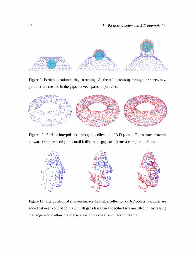
of this stretching rule in action is shown in Figure 9, where a ball pushing against a sheet

stretches it to the point where new particles are added.

The second (growing) rule allows particles to be added in all directions with respect to

7 Particle creation and 3-D interpolation 17

a particle’s localx-y plane. The rule is generalized to allow a minimum and maximum

number of neighbors and to limit growth in regions of few neighboring particles, such as

at the edge of a surface. The rule counts the number of immediate neighborsnN to see

if it falls within a valid rangenmin nN nmax. It also computes the angles between

successive neighbors∆i i1i using the particle’s local coordinate frame, and checks

if these fall within a suitable rangemin ∆i max. If these conditions are met, one or

more particles are created in the gap. In general, a sheet at equilibrium will have interior

particles with six neighbors spaced 60 apart while edge particles will have four neighbors

with one pair of neighbors 180 apart.

With these two rules, we can automatically build a surface from collections of 3-D

points. We create particles at each sample location and fix their positions and orientations.

We then start filling in gaps by growing particles away from isolated points and edges. After

a rough surface approximation is complete we can release the original sampled particles

to smooth the final surface thereby eliminating excessive noise. If the set of data points

is reasonably distributed, this approach will result in a smooth continuous closed surface

(Figure 10). The fitted surface is not limited to a particular topology, unlike previous 3-D

surface fitting models such as [Terzopouloset al., 1987b; Milleret al., 1991].

We can also fit surfaces to data that does not originate from closed surfaces, such as stereo

range data [Barnard and Fischler, 1982; Fua and Sander, 1992; Szeliski, 1991]. Simply

growing particles away from the sample points poses several problems. For example, if we

allow growth in all directions, the surface may grow indefinitely at the edges, whereas if we

limit the growth at edges, we may not be able to fill in certain gaps. Instead, we apply the

stretching heuristic to effectively interpolate the surface between the sample points (Figure

11). When the surface being reconstructed has holes or gaps, we can control the size of

gaps that are filled in by limiting the search range. This is evident in Figure 11, where the

cheek and neck regions have few samples and were therefore not reconstructed. We could

have easily filled in these regions by using a larger search range.

18 7 Particle creation and 3-D interpolation

Figure 9: Particle creation during stretching. As the ball pushes up through the sheet, new

particles are created in the gaps between pairs of particles.

Figure 10: Surface interpolation through a collection of 3-D points. The surface extends

outward from the seed points until it fills in the gaps and forms a complete surface.

Figure 11: Interpolation of an open surface through a collection of 3-D points. Particles are

added between control points until all gaps less than a specified size are filled in. Increasing

the range would allow the sparse areas of the cheek and neck to filled in.

8 Geometric Modeling Applications 19

Figure 12: Varying the surface characteristics to change its behavior: (a) cloth draping, (b)

plastic deformation, (c) tearing.

8 Geometric Modeling Applications

The particle-based surface models we have presented can be used in a wide range of

geometric modeling and animation applications. These include applications which have

been previously demonstrated with physically-based deformable surface models, such as

cloth draping [Weil, 1986; Terzopouloset al., 1987b; Breenet al., 1991] (Figure 12a),

plastic surface deformations [Terzopoulos and Fleischer, 1988b] (Figure 12b), and tearing

[Terzopoulos and Fleischer, 1988b] (Figure 12c).

Using our surface model as an interactive design tool we can spray collections of points

into space to form elastic sheets, shape them under interactive user control, and then freeze

them into the desired final configuration. We can create any desired topology with this

technique. For example, we can form a flat sheet into an object with a stem and then

a handle (Figure 13). Forming such surface with traditional spline patches is a difficult

problem that requires careful attention to patch continuities [Loop and DeRose, 1990]. To

make this example work, we add the concept ofheatingthe surface near the tool [Tonnesen,

1991] and only allowing the hot parts of the surface to deform and stretch. Without this

modification, the extruded part of the surface has a tendency to “pinch off” similar to how

soap bubbles pinch before breaking away. As another example, we can start with a sphere,

20 8 Geometric Modeling Applications

Figure 13: Forming a complex object. The initial surface is deformed upwards and then

looped around. The new topology (a handle) is created automatically.

Figure 14: Deformation from sphere to torus using two spherical shaping tools. The final

view is from the side, showing the toroidal shape.

8 Geometric Modeling Applications 21

and by pushing in the two ends, form it into a torus (Fig 14). New particles are created inside

the torus due to stretching during the formation process, and some old sphere particles are

deleted when trapped between the two shaping tools.

Another interesting application of our oriented particle systems is the interpolation and

extrapolation of sparse 3-D data. This is a difficult problem when the topology or rough

shape of the surface to be fitted is unknown. As described in the previous section, oriented

particles provide a solution by extending the surface out from known data points. We

believe that these techniques will be particularly useful in machine vision applications

where it can be used to interpolate sparse position measurements available from stereo or

tactile sensing [Szeliski, 1991].

A direct extension of our surface fitting procedure is to add a potential function that

induces a torque around the localz axis. This torque can be used to force thex andy axes

to align themselves in the directions of minimum and maximum curvature. For example,

the potential term (expressed in local coordinates)

Sx y z x2z x y z 14

encourages thex axis to align itself in the direction of smallest curvature (greatest negative

curvature). Similarly, the potential term

Sx y z x2z2x y z 15

encourages thex axis to align itself in the direction of smallestabsolutecurvature. In

order not to disturb the original dynamics of the surface, the above potential is used only

to compute a torque around the localz axis. Adding these curvature-based torques to our

particle system results in a covering of the surface with local coordinate frames that indicate

the principal directions of the surface at each point (Figure 15). The resulting system of

oriented particles resembles the collection of interacting Darboux frames used by Sander

and Zucker [1990].

22 9 Discussion

Figure 15: The spin torque potentialS forces the local coordinate frames to align with the

minimum and maximum curvatures of the surface (short and long axes, respectively). The

left and right images are before and after the addition ofS.

9 Discussion

The particle-based surface model we have developed has a number of advantages over

traditional spline-based and physically-based surface models. Particle-based surfaces are

easy to shape, extend, join, and separate. By adjusting the relative strengths of various

potential functions, the surface’s resistance to stretching, bending, or variation in curvature

can all be controlled. The topology of particle-based surfaces can easily be modified, as can

the sampling density, and surfaces can be fitted to arbitrary collections of 3-D data points.

One limitation of particle-based surfaces is that it is harder to achieve exact analytic

(mathematical) control over the shape of the surface. For example, the torus shaped from

a sphere is not circularly symmetric, due to the discretization effects of the relatively small

number of particles. This behavior could be remedied by adding additional constraints

in the form of extra potentials, e.g., a circular symmetry potential for the torus. Particle-

based surfaces also require more computation to simulate their dynamics than spline-based

surfaces; the latter may therefore be more appropriate when maximum shape flexibility is

not paramount.

One could easily envision a hybrid system where spline or other parametric surfaces

10 Conclusion 23

co-exist with particle-based surfaces, using each system’s relative advantages where appro-

priate. For example, particle-based surface patches could be added to a constructive solid

geometry (CSG) modeling system to perform fileting at part junctions.

In future work, we will apply particle-based surfaces to iso-surfaces in volumetric data

sets. When combined with the stretching heuristic for particle creation and an inflation

force, this model would behave in a manner similar to the geometrically deformed models

(GDM) of [Miller et al., 1991]. We could extend this idea by tracking a volumetric data set

through time by deforming the particle surface from one frame to the next.

In another application, we could distribute the particles over the surface of a CAD

model and allow the particles to change position and orientation while remaining on the

surface of the model, thereby creating a uniform triangulation of the surface. Figure 11

shows how this can be achieved, even without the presence of the CAD model surface to

attract the particles. A curvature-dependent adaptive meshing of the surface could also

be obtained by locally adjusting the preferred inter-particle spacing. This would be very

useful for efficiently rendering parametric surfaces such as NURBS.

10 Conclusion

In this paper, we have developed a particle-based model of deformable surfaces. Our

new model, which is based on oriented particles with new interaction potentials, has

characteristics of both physically-based surface models and of particle systems. It can be

used to model smooth, elastic, moldable surfaces, like traditional splines, and it allows for

arbitrary interactions and topologies, like particle systems.

Like previous deformable surface models, our new particle-based surfaces can simulate

cloth, elastic and plastic films, and other deformable surfaces. The ability to grow new

particles gives these model more fluid-like properties which extend the range of interactions.

For example, the surfaces can be joined and cut at arbitrary locations. These characteristics

24 10 Conclusion

make particle-based surfaces a powerful new tool for the interactive construction and

modeling of free-form surfaces.

Oriented particles can also be used to automatically fit a surface to sparse 3-D data

even when the topology of the surface is unknown. Both open and closed surfaces can

be reconstructed, either with or without holes. The reconstructed model can be used as

the starting point to interactively create a new shape and then animated within a virtual

environment. Thus oriented particle systems provide a convenient interface between surface

reconstruction in computer vision, free form modeling in computer graphics, and animation.

References

[Appel, 1985] A. Appel. An efficient algorithm for many-body simulations.SIAM J. Sci.

Stat. Comput., 6(1), 1985.

[Barnard and Fischler, 1982] S. T. Barnard and M. A. Fischler. Computational stereo.

Computing Surveys, 14(4):553–572, December 1982.

[Bartels and Beatty, 1989] R. H. Bartels and J. C. Beatty. A technique for the direct

manipulation of spline curves. InGraphics Interface ’89, pages 33–39, June 1989.

[Bartelset al., 1987] R. H. Bartels, J. C. Beatty, and B. A. Barsky.An Introduction to

Splines for use in Computer Graphics and Geeometric Modeling. Morgan Kaufmann

Publishers, Los Altos, California, 1987.

[Blinn, 1982a] J. F. Blinn. Light reflection functions for simulation of clouds and dusty

surfaces.Computer Graphics (SIGGRAPH’82), 16(3):21–29, July 1982.

[Blinn, 1982b] J. F. Blinn. A generalization of algebraic surface drawing.ACM Transac-

tions on Graphics, 1(3):235–256, July 1982.

[Boissonat, 1984] J.-D. Boissonat. Representing 2D and 3D shapes with the Delaunay

triangulation. InSeventh International Conference on Pattern Recognition (ICPR’84),

10 Conclusion 25

pages 745–748, Montreal, Canada, July 1984.

[Breenet al., 1991] D. E. Breen, D. H. House, and P. H. Getto. A particle-based com-

putational model of cloth draping behavior. In N. M. Patrikalakis, editor,Scientific

Visualization of Physical Phenomena, pages 113–134, Springer-Verlag, New York,

1991.

[Celniker and Gossard, 1991] G. Celniker and D. Gossard. Deformable curve and surface

finite-elements for free-form shape design.Computer Graphics (SIGGRAPH’91),

25(4):257–266, July 1991.

[Coquillart, 1990] S. Coquillart. Extended free-form deformations: A sculpturing tool

for 3d geometric modeling.Computer Graphics (SIGGRAPH’90), 24(4):187–196,

August 1990.

[Farin, 1990] G. E. Farin.Curves and Surfaces for Computer Aided Geometric Design: A

Practical Guide. Academic Press, Boston, Massachusetts, 2nd edition, 1990.

[Fua and Sander, 1992] P. Fua and P. Sander. Reconstructing surfaces from unstructured 3d

points. InSecond European Conference on Computer Vision (ECCV’90), (submitted)

1992.

[Hersh, 1987] J. Hersh.Soft Object Extensions to The Clockworks system. Technical Re-

port TR-87054, Rensselaer Design Research Center, Rensselaer Polytechnic Institute,

Troy, New York, 1987.

[Hockney and Eastwood, 1988] R. W. Hockney and J. W. Eastwood.Computer Simulation

using Particles. McGraw-Hill Inc., New York, 1988.

[Kasset al., 1988] M. Kass, A. Witkin, and D. Terzopoulos. Snakes: Active contour

models.International Journal of Computer Vision, 1(4):321–331, January 1988.

[Loop and DeRose, 1990] C. Loop and T. DeRose. Generalized B-spline surfaces of arbi-

trary topology.Computer Graphics (SIGGRAPH’90), 24(4):347–356, August 1990.

26 10 Conclusion

[Miller and Pearce, 1989] G. Miller and A. Pearce. Globular dynamics: A connected

particle system for animating viscous fluids. InSIGGRAPH ’89, Course 30 notes:

Topics in Physically-based Modeling, pages R1 – R23, SIGGRAPH, August 1989.

Boston, Massachusetts.

[Miller et al., 1991] J. V. Miller, D. E. Breen, W. E. Lorensen, R. M. O’Bara, and M. J.

Wozny. Geometrically deformed models: A method of extracting closed geometric

models from volume data.Computer Graphics (SIGGRAPH’91), 25(4):217–226,

July 1991.

[Platt and Barr, 1988] J. C. Platt and A. H. Barr. Constraint methods for flexible models.

Computer Graphics (SIGGRAPH’88), 22(4):279–288, August 1988.

[Presset al., 1988] W. H. Press, B. P. Flannery, S. A. Teukolsky, and W. T. Vetterling.

Numerical Recipes in C: The Art of Scientific Computing. Cambridge University

Press, Cambridge, England, 1988.

[Reeves, 1983] W. T. Reeves. Particle systems—a technique for modeling a class of fuzzy

objects.ACM Transactions of Graphics, 2(2):91–108, April 1983.

[Reeves and Blau, 1985] W. T. Reeves and R. Blau. Approximate and probabilistic algo-

rithms for shading and rendering structured particle systems.Computer Graphics,

19(3):313–322, July 1985.

[Sachset al., 1991] E. Sachs, A. Roberts, and D. Stoops. 3-draw: A tool for designing 3d

shapes.IEEE Computer Graphics & Applications, 11(6):18–26, November 1991.

[Samet, 1989] H. Samet.The Design and Analysis of Spatial Data Structures. Addison-

Wesley, Reading, Massachusetts, 1989.

[Sander and Zucker, 1990] P. T. Sander and S. W. Zucker. Inferring surface trace and

differential structure from 3-D images.IEEE Transactions on Pattern Analysis and

Machine Intelligence, 12(9):833–854, September 1990.

[Shoemake, 1985] K. Shoemake. Animating rotation with quaternion curves.Computer

10 Conclusion 27

Graphics (SIGGRAPH’85), 19(3):245–2540, July 1985.

[Sims, 1990] K. Sims. Particle animation and rendering using data parallel computation.

Computer Graphics (SIGGRAPH’90), 24(4):405–413, August 1990.

[Szeliski, 1991] R. Szeliski. Shape from rotation. InIEEE Computer Society Confer-

ence on Computer Vision and Pattern Recognition (CVPR’91), pages 625–630, IEEE

Computer Society Press, Maui, Hawaii, June 1991.

[Terzopoulos, 1988] D. Terzopoulos. The computation of visible-surface representations.

IEEE Transactions on Pattern Analysis and Machine Intelligence, PAMI-10(4):417–

438, July 1988.

[Terzopoulos and Fleischer, 1988a] D. Terzopoulos and K. Fleischer. Deformable models.

The Visual Computer, 4(6):306–331, December 1988.

[Terzopoulos and Fleischer, 1988b] D. Terzopoulos and K. Fleischer. Modeling inelas-

tic deformations: Visoelasticity, plasticity, fracture.Computer Graphics (SIG-

GRAPH’88), 22(4):269–278, August 1988.

[Terzopouloset al., 1989] D. Terzopoulos, J. Platt, and K. Fleischer. From goop to

glop: Heating and melting deformable models. InProceedings Graphics Interface,

pages 219–226, Graphics Interface, June 1989.

[Terzopouloset al., 1987a] D. Terzopoulos, A. Witkin, and M. Kass. Symmetry-seeking

models and 3D object reconstruction.International Journal of Computer Vision,

1(3):211–221, October 1987.

[Terzopouloset al., 1987b] D. Terzopoulos, J. Platt, A. Barr, and K. Fleischer. Elastically

deformable models.Computer Graphics (SIGGRAPH’87), 21(4):205–214, July 1987.

[Tonnesen, 1989] D. Tonnesen.Ray-tracing implicit surfaces resulting from the summation

of bounded polynomial functions. Technical Report TR-89003, Rensselaer Design

Research Center, Rensselaer Polytechnic Institute, Troy, New York, 1989.

28 A Finite element analysis of local deformation energies

[Tonnesen, 1991] D. Tonnesen. Modeling liquids and solids using thermal particles. In

Graphics Interface ’91, pages 255–262, 1991.

[Weil, 1986] J. Weil. The synthesis of cloth objects.Computer Graphics (SIGGRAPH’86),

20(4):49–54, August 1986.

[Witkin and Welch, 1990] A. Witkin and W. Welch. Fast animation and control of nonrigid

structures.Computer Graphics (SIGGRAPH’90), 24(4):243–252, August 1990.

[Wolfram, 1988] S. Wolfram.Mathematica: A System for Doing Mathematics by Com-

puter. Addison-Wesley, Redwood City, California, 1988.

[Wyvill et al., 1986] B. Wyvill, C. McPheeters, and G. Wyvill. Data structures for soft

objects.The Visual Computer, 2:227–234, 1986.

A Finite element analysis of local deformation energies

To derive the local oriented particle interaction potentials, we analyze the deformation

energies of a triangular surface patch defined by three neighboring particles. For this

analysis, we assume that the particles are in an equilateral configuration with locations

00, h0 and12p

32 in the x y plane. We examine the small-deflection case

where the height from the plane,z fx y, describes the local shape of the surface.

Both of these assumptions are reasonable for our surfaces, since the Lennard-Jones forces

favor locally hexagonal arrangements, and a sufficiently high sampling density will ensure

small deflections. For an analysis of the general parametric patch case, see [Celniker and

Gossard, 1991].

We use a cubic function forfx y since it can be specified by the heights and gradients

at the three cornersfzi pi qi i 0 2g and the heightz3 of a “bubble” node in the

middle of a triangle. We choose thex y plane to pass through the three particles, which

gives us a height of 0 at all three corners.

A Finite element analysis of local deformation energies 29

To compute the deformation energies, we take integrals of squared derivatives over the

triangle. For example, we can compute the area of the triangle from

A Z Z q

1 f2x f2

y dx dy p

34h2

12

Z Zf2x f2

y dx dy

We can compute the average Gaussian curvature from

C 12

Z Zf2xx 2f2

xy f2yy dx dy

and the average variation in curvature from

V 12

Z Zf2xxx 3f2

xxy 3f2xyy f2

yyy dx dy

These three integrals can be thought of as corresponding to the stretching, bending, and “un-

dulation” energies of the surface. After some algebraic manipulation, which we performed

using MathematicaTM[Wolfram, 1988], we obtain formulas for the above three equations in

terms of the corner gradient valuesfpi qig and the bubble heightz3 (the expressions are

quadratic in these variables).

In our oriented particle system, we desire to have interactions only between pairs

of particles. Since we are only interested in the energies involving two particles, say

the particles which controlp0 q0 andp1 q1, we minimize the quadratic energies with

respect to thep2, q2, andz3 variables (this results in lower energies than arbitrarily setting

these unknown quantities to 0, which would be the effect of ignoring these other terms).

To further simplify the energies, we express them in terms of averages and differences of

gradients

p p0 p12 q q0 q12

p p0 p12 q q0 q12

Again, applying the tools in MathematicaTM, we obtain

V h26p

3p2 (16)

30 A Finite element analysis of local deformation energies

C

p3

2268567p2

316p2

8p

3pq 48q2 315q2

(17)

A h2

p3

41

6003281880

p2 (18)

How do we compute these quantities given the state of two particles, i.e., their positions

and orientations? We must first write the scalar quantitiesp0, p1, q0, andq1 in terms ofni,

nj andrij. We identifyrij with thex direction in our local plane, and thus compute

p0 ni rij and p1 nj rij

for small values ofp0 andp1. Choosing they direction is more difficult if we wish to keep

the interactions pairwise, since we cannot use the location of the third point defining the

triangle. A simple choice is to choose the localz direction along the average normal vector

ni nj2, which leads to the equations

q ni nj

2

dni nj

2 rij 0

q ni nj

2

dni nj

2 rij

p2 q2

14kni njk2

We are now in a position to relate the finite element based measures for curvature and

variation in curvature to the co-planarity, co-normality, and co-circularity measures. The

variation in curvatureV (17) corresponds directly to the co-circularityC (8). The curvature

itself C (18) can be written as a sum of the co-circularity potential and the co-normality

potentialN (7). The co-planarity potential is therefore not needed to write a curvature-

based energy measure. It is useful, however, when used in isolation, since it corresponds

to terms of the form

p20 p2

1 p2 p2

While the area-based measureA (18) is too complicated to warrant direct implementation,

finite rest area behavior is simulated by the Lennard-Jones interaction potentialLJ.

B Computation of internal forces 31

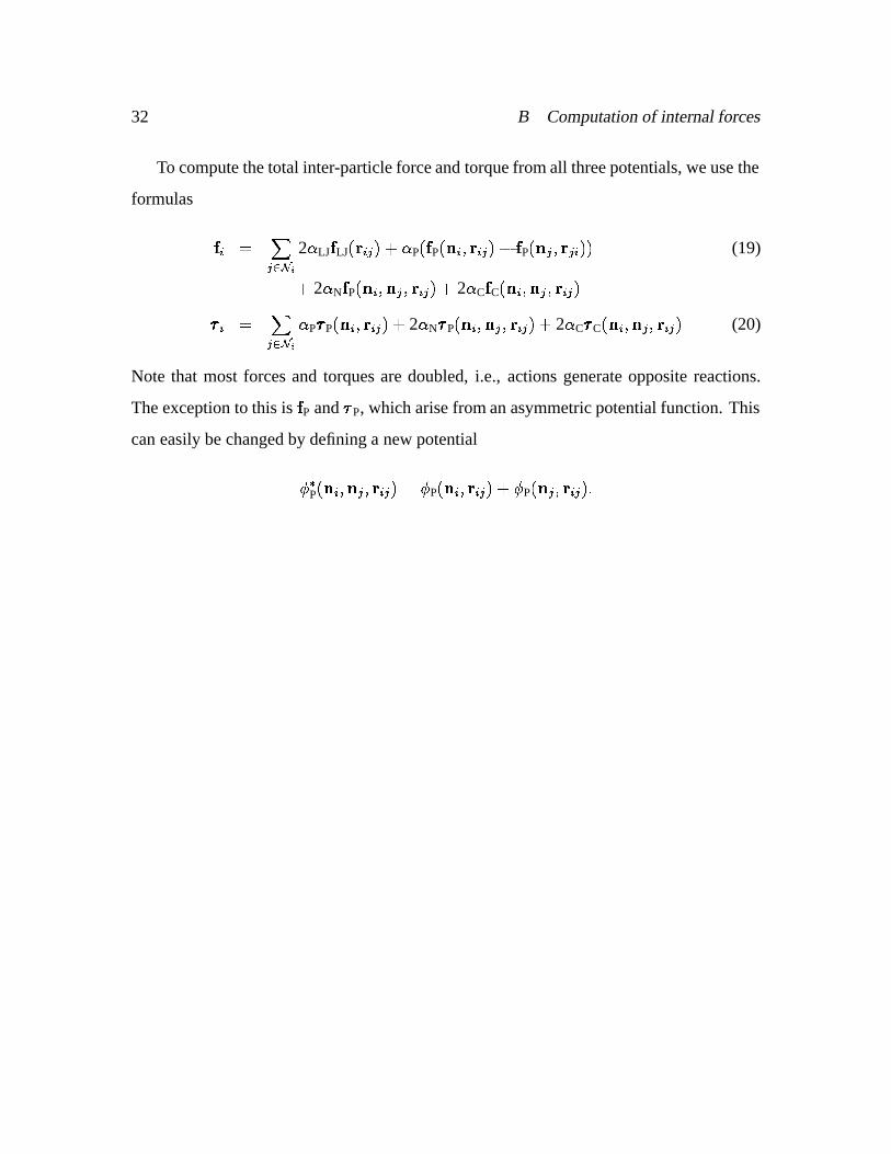
B Computation of internal forces

To compute the internal inter-particle forces and torques, we compute the variation of inter-

particle potentials with respect to particle positions and orientations. We can compute these

forces and torques using the equations

f rp and rpp v v

r and rn v n v

where is the incremental change in orientationR, i.e., _n n.

Applying these equations to the various internal potentials, we obtain

fLJrij rij LJkrijkfPni rij nini rijkrijk rijni rij2krijkPni rij rij nini rijkrijk rij fP

fNninj rij rijkni njk2krijkNninj rij ni nj ni krijk ni nj krijkfCninj rij nini nj rijkrijk rijni nj rij2krijkCninj rij rij nini nj rijkrijk rij fC

whererij is the unit vector alongrij. These forces have the following simple physical

interpretations.

The co-planarity potential gives rise to a force parallel to the particle normal and

proportional to the distance between the neighboring particle and the local tangent plane.

The second term in the force, which can often be ignored, arises from the gradient of the

spatial weighting function. The cross product of this force with the inter-particle vector

produces a torque on the particle. The co-normality potential produces a torque proportional

to the cross-product of the two particle normals, which acts to lign up the normals. The

co-circularity force is similar to the co-planarity force, except that the local tangent plane

is defined from the average of the two normal vectors.

32 B Computation of internal forces

To compute the total inter-particle force and torque from all three potentials, we use the

formulas

fi XjNi

2LJfLJrij PfPni rij fPnj rji (19)

2NfPninj rij 2CfCninj rij

i XjNi

PPni rij 2NPninj rij 2CCninj rij (20)

Note that most forces and torques are doubled, i.e., actions generate opposite reactions.

The exception to this isfP andP, which arise from an asymmetric potential function. This

can easily be changed by defining a new potential

Pninj rij Pni rij Pnj rij