www.sciencemag.org/cgi/content/full/331/6022/1333/DC1

Supporting Online Material for

Function of Rhodopsin in Temperature Discrimination in Drosophila

Wei L. Shen, Young Kwon, Abidemi A. Adegbola, Junjie Luo, Andrew Chess, Craig Montell

*To whom correspondence should be addressed. E-mail: cmontell@jhmi.edu

Published 11 March 2011, Science 331, 1333 (2011) DOI: 10.1126/science.1198904

This PDF file includes

Materials and Methods Figs. S1 to S8 Tables S1 to S17 References

Other Supporting Online Material for this manuscript includes the following: (available at www.sciencemag.org/cgi/content/full/331/6022/1333/DC1)

Movie S1

1

Supporting Online Material for

Function of rhodopsin in temperature

discrimination in Drosophila

Wei L. Shen, Young Kwon, Abidemi A. Adegbola,

Junjie Luo, Andrew Chess and Craig Montell*

*Correspondence: e-mail, cmontell@jhmi.edu

This PDF file includes:

Materials and Methods

Figures S1-8

Movie S1 legend

Tables S1-18

References

2

Materials and Methods Sources of fly Stocks

w1118 was used as the wild-type control. The following flies were obtained from the Bloomington Stock center (stock numbers are indicated): ninaEI17 (#5701), ninaE1 (#1946), ninaEP318 (#3531), ninaEP332 (#1613), ninaE Df (#9479), ninaE-GAL4 (#8691), norpAP24 (#9048), rdgC306 (#3601), UAS-dicer2 (#24644) and UAS-5-HT2.DCIII (#24506). The following stocks were provided by the indicated investigators: ninaEP352, ninaEP354 and ninaEP362 (D.F Ready), trpA1-GAL4 (P. Garrity), ninaE-rh2, ninaE-rh3 and ninaE-rh4 (C.S Zuker), ninaE-rh5 and ninaE-rh6 (S.G. Britt). ninaE-norpA was generated in our laboratory. The following stocks were created in our laboratory and are available from the Bloomington Stock Center (stock numbers are indicated): trpA11 (#26504) and santa maria1(#24520). The following RNAi lines were from the Harvard Transgenic RNAi Project (TRiP: http://www.flyrnai.org/TRiP-HOME.html): ninaE (JF01438), G49B (JF01209), norpA (JF01585), trpA1 (JF01360). Generation of transgenic flies

We generated the UAS-ninaE line by cloning the ninaE cDNA into the pUAST vector (1), and by selecting for w+ transformants. The ninaE-Opn4 line was generated (T Wang and Montell, unpublished) by inserting the mouse Opn4 cDNA (provided by K.W. Yau) into pCaspeRhs and selecting for w+ transformants (2). The trpl-mCherry was a fusion between a 4.3 kb trpl promoter and the cDNA encoding mCherry tagged with a C-terminal Ki-ras membrane targeting motif. The trpl-mCherry construct was subcloned into pCasper4 and w+ transformants were selected. The primers were: trpl promoter forward: ATTTGCGGCCGCCCAGGCTATTGG CATAAAAGTCG; reverse: CGCGGATCCTTGAAGGCGAAAACCCGC. mCherry forward: ATT GCGGCCGCATGGTGAGCAAGGGCGAGGAGG; reverse: CTGGGATCCTTACATAATTACA CACTTGTA CAGCTCGTCCATGCC. Media for feeding

All-trans-retinal was purchased from Sigma (#R2500). Flies were reared at 25°C on standard cornmeal-yeast medium under a 12-h light/12-h dark cycle unless indicated otherwise. The vitamin A depleted medium (Fig. 2A) consisted of: 240 ml H2O, 10 g dry yeast, 10 g glucose, 12 g rice powder, 2 g agar, 60 mg cholesterol, 3 ml 10% butyl p-hydroxybenzoate and 0.8 ml propionic acid. To prepare the retinal plus (R+) food, all trans-retinal was dissolved in ethanol and then added to the vitamin A depleted medium (Fig. 2A) or to instant fly food (Carolina Biological Supply Co; Fig. 2B) at a final concentration of 200 M. Temperature two-way choice assays

We described the two-way choice assay previously (3) in detail: (http://www.natureprotocols.com/2008/07/28/assaying_thermotaxis_behavior.php). Briefly, we used plexiglass plate covers (8.38 x 5.83cm) (Fig. S1A) from 6 x 12 mini trays (Nunc 136528) coated with 7 ml of 2% agarose. The plates were placed on top of two adjacent aluminum blocks, which were separated by a plastic spacer. The blocks were individually temperature controlled using circulating water (Thomas Scientific, 9106). We monitored the surface temperatures on the center of each side of the test plate using microprobe thermometers (BAT-12, Physitemp Instruments) with probes (IT-21, Physitemp Instruments). Water was gently sprayed to keep the agarose surface from drying. We released 40-100 larvae (~95% 3rd

3 instar) at the middle of the plates (Fig. S1A), and conducted the experiments under dim ambient lights (0.035 mW/cm2) unless indicated otherwise. The larvae on each side of the plates were scored after 10 min. and the preference indexes (PIs) were calculated as follows: (number of larvae on the 18°C side) – (number of larvae on the side with the alternative temperature)/(total number of larvae on both sides of the test plate).

For the thermotaxis assay in the presence of light (Fig. 2D and Fig. S4B), we used the same test plate as above and held it at a given temperature (Fig. S4A). Lights were piped from a Lumina light source (Chiu Technical Co), which illuminated the test plate vertically through a filter ~17 cm above the plate. A BG3 glass filter (Schott) was used for blue light, and an OG590 glass filter (Schott) was used for orange light. For white light, instead of using a filter, we placed a water-filled 150 mm Petri dish cover in the light path to minimize heating. After the plate temperature reached equilibrium, we monitored the plate surface temperature during the 10 min assay. Light illumination did not change the surface temperature (<0.2°C). Turning behavioral assays

Turning increased among wild-type larvae as they crossed the border from the 18°C zone to the 24°C zone (movie S1). In order to quantify this behavior, we measured the distance traveled before the first turn using the same plates employed for the thermal choice assay. We divided the 24°C zone with 20 parallel lines, which were spaced 2 mm apart. We released the larvae in the 18°C zone and then followed those larvae which moved perpendicular (5°) to the 20 lines (Fig. 4A). The last lines crossed before the larvae made the first turn were tabulated. We also quantified the first turn at 18°C when larvae were released into the 24°C zone and moved into the 18° zone. Moving trace analyses

To track larval movements (Fig. S6A), we videotaped the animals using a Canon PowerShot SD790 IS camera (1 frame/sec for 10 min) and downloaded the movies into QuickTime Pro. We manually traced the larval movements using software available at the National Institutes of Health (ImageJ 1.42 with plugin MTrackJ). The coordinates (x and y) for each time point were imported into Excel 2007 (Microsoft) to create the traces shown in Fig. S6A. To measure the speed and turn rates at different temperatures, we videotaped larvae on plates, which were maintained at a uniform temperature indicated in Fig. S6, B and C. The speeds were calculated from 50 traces. Speed is equal to the distance traveled (mm) over time (s). We counted turns (movie S1) from 50 traces that lasted longer than 15 s. RT-PCR from manually dissected cells

We obtained individual GFP-positive larval body wall neurons and anterior neurons by micromanipulation and dissection under a dissecting microscope (Carl Zeiss Stemi SV 11, 200X magnification) from UAS-YC3.6.;trpA1-GAL4 3rd instar larvae. GFP-negative tissue was obtained in parallel. Usually 5-10 cells were in each group. Therefore, the GFP-positive sample consisted of one GFP-positive neuron and 4-9 GFP-negative cells, and the GFP-negative controls consisted of 5-10 cells devoid of any GFP positive cell. Cell lysis was carried out using the Invitrogen CellsDirect Resuspension/Lysis buffer (#11739010) followed by multiplex RT-PCR. To perform the RT-PCR, we used the Qiagen OneStep RT-PCR kit (#210210) with primers for trpA1, norpA, G49B and ninaE that spanned introns, allowing us to distinguish between RNA and genomic DNA-derived products. Following the RT-PCR, the samples were split into four aliquots. 1 l of each was used for a second round of PCR carried out with the Promega GoTaq Hot-Start PCR kit (# M5001) in four separate reactions, one for each gene.

4 For ninaE, the same PCR primers were used to perform the second round of PCR. For the other three genes, the second round primers were nested. Each round of PCR was 35 cycles. We carried out parallel reactions on GFP-negative control tissue, and included Rp49 as a control. The Rp49 analysis was carried out on 1/4 of the cell lysate from each sample, while 3/4 of the lysate was used for a multiplex RT-PCR reaction.

Cycling parameters for the first round RT-PCR were as follows: reverse transcription, 30 min at 50°; initial PCR activation step 15 min at 95°; 3-step cycling: denaturation 30 sec at 94°, annealing 45 sec at 58°, extension 1 min at 72° for 35 cycles, and final extension 72° for 10 min. Cycling parameters for the second round PCR reaction were as follows: initial denaturation step 2.5 min at 94°; 3-step cycling: denaturation 30 sec at 94°, annealing 45 sec at 58°, extension 45 sec at 72° for 35 cycles, and final extension 72° for 10 min.

The internal primer pairs used and the expected sizes of the PCR products (base pairs, bp) generated from RNA (cDNA) and genomic DNA (gDNA) were: ninaE: (cDNA, 201; gDNA, 376) forward: CGCTACCAAGTGATCGTCAA; reverse: GTATGAGCGTGGGTTCCAGT. norpA: (cDNA, 410; gDNA, 869) forward: AGTTCCGTGGAAATGTACCG; reverse: CAGAGCTCCAACTCGACCTT. trpA1: (cDNA, 208; gDNA, 699) forward: ACATGACACCGACATGGAGA; reverse: TTAGTTGCCAGCAACGTTTT. G49B: (cDNA, 275; gDNA) forward: GCGATCCGAGAGAAGAAAGT; reverse: CTCGCTGAGGACCATCGTAT. There were no genomic products expected due to the fact that the reverse primer spanned a splice junction. If genomic amplification were to occur, the expected size would be 337 bp. rp49: (cDNA, 464; gDNA, 526) forward: ATGCTAAGCTGTCGCACAAA; reverse: ATGGTGCTGCTATCCCAATC. There were no genomic products expected due to the fact that the forward primer spanned a splice junction. If genomic amplification were to occur, the expected size would be 526 bp.

The external primers used were: norpA: (cDNA 550; gDNA, 1009) forward: ACGCACCTGTATTCCTGGAC; reverse: GTTTTGAGTTCGCCCTTCAG. trpA1: (cDNA 380 ; gDNA, 871) forward: ATGTGGATGCTGAGGTTTCC; reverse: TGGAATCGTGTGTGTTTGCT. G49B: (cDNA 591; gDNA 1468) forward: AATGGTAGACGTCGGTGGTC; reverse: CGCTCGCTTCTCAATTCTTC.

Electroretinogram recordings We performed electroretinograms (ERGs) using two glass microelectrodes filled with

Ringer's solution. We inserted the electrodes in drops of electrode cream on the surfaces of the compound eye and the thorax. The light source was a Newport light projector (model 765). We amplified the signals using a Warner Instruments electrometer IE-210, and recorded the light responses with a Powerlab 4/30 analog-to-digital converter (AD Instruments) in conjunction with the Lab Chart version 6.1 program (AD Instruments). The recordings were performed at room temperature. Imaging

To examine GFP fluorescence directly, wondering 3rd instar larvae were washed and heat-killed at 65°C for 30 s. Larvae were sandwiched between a coverslip and a slide using vacuum grease. Z-stack of images were collected using a Carl Zeiss LSM 510 confocal microscope. The pictures shown in Fig. 3C, Fig. S5 and Fig. S7A are 2-D projections from z-stacks.

5

Figure S1

Figure S1. Setup and map of ninaE mutations. (A) Diagram showing the setup used for thermotactic behavior. Larvae were released in the middle of a test plate (8.38 x 5.83 cm) and allowed to choose between 18°C and the alternative temperature for 10 min. The number of larvae in each of the two temperature zones were tabulated and used to calculate the preference index (PI). A PI of 0 results if there is no bias for either temperature. 100% preferences for 18°C or the alternative temperature results in PIs of 1.0 and -1.0 respectively. (B) Cartoon showing the position of the ninaEP332 mutation and several other ninaE mutations (4, 5). See Flybase for ninaE1: http://flybase.org/reports/FBal0013006.html. The numbers represent the amino acids in Rh1. The wild-type and altered residues are shown to the left and right respectively. The ninaEP352 allele might have another mutation (G334E): http://flybase.org/reports/FBal0013014.html. Mutations in ninaEP354 and ninaEP362 have not been mapped.

6

Figure S2

Figure S2. Thermal choices of ninaE mutants and santa maria1. (A) 18°C versus 14°C selection. (B) 18°C versus 26°C. (C) Binary choices of ninaEP332 and controls between 18°C and 20-24°C. (D) Thermal preferences of santa maria1. The larvae were given a choice between 18°C and temperatures ranging from 14°C to 32°C. The error bars represent S.E.M.s. Differences were relative to wild-type (*; p<0.05; C, Dunnett’s ANOVA; D, Tukey’s ANOVA). See Table S2,14,15 for detailed statistics.

7

Figure S3

Figure S3. Effects on thermotaxis (18° versus 24°C) resulting from knockdown of ninaE by RNAi. The error bars show the S.E.M.s. *; p<0.05, Tukey’s ANOVA test. See Table S10 for detailed statistics.

8

Figure S4

9 Figure S4. Effects of light on thermotaxis. (A) Setup for illumination of plates for thermotaxis assays. To illuminate a test plate with either blue or orange light, light was piped from a Lumina light source (Chiu Technical Co) and passed through a glass wavelength filter. For white light, we placed a water-filled 150 mm Petri dish cover in the position of the light filter to minimize heating. The light intensities were: ambient, ~0.035 mW/cm2; white, 11.5 mW/cm2; blue, 6.75 mW/cm2; orange, 10.9 mW/cm2. The setup was covered with black cloth during the experiments. (B) Influences of light on thermotaxis. Wild-type and blind larvae (norpAP24;; trpA1-GAL4/UAS-norpA) were assayed at room temperature (RT, ~20°C) or at the indicated temperatures (18°-23°C) and light conditions. The error bars represent S.E.M.s. For each genotype, we used Tukey’s ANOVA to compare the PIs of phototaxis at RT and used Dunnett’s ANOVA to compare PIs of 18°- 23°C selection under different light condition. The first statistical significance was relative to wild-type’s dark-versus-white PI. The 2nd and 3rd were relative to wild-type PIs at 18° versus 23°C under ambient light. See Table S8 for detailed statistics.

10

Figure S5

Figure S5. The trpA1-GAL4 is not expressed in the Bolwig’s organ (BO) in 3rd instar larvae. As a marker for the BO, we used a transgene that expressed mCherry under the control of the trpl promoter (trpl-mCherry). The larvae also contained the UAS-mCD8-GFP reporter, which was expressed under the control of the trpA1-GAL4. The genotype of the larvae was: trpl-mCherry/+,UAS-mCD8-GFP/+;trpA1-GAL4/+. The image on the right is a merge of the bright field and the windows showing expression of mCherry and GFP. The gain was increased in the GFP window to show that GFP was not expressed in the BO.

11

Figure S6

Figure S6. Temperature-dependent turning and rates of movement. (A) Tracking turning of individual larvae. Two typical traces are shown for wild-type larvae and each of the indicated mutants. The black dots represent the starting points. (B and C) The entire plates were held at a single temperature as indicated. (B) Movement speeds. (C) Turning rates. The error bars show the S.E.M.s. See Tables S16-17 for detailed statistics.

12

Figure S7

13 Figure S7. Neurons expressing the trpA1 reporter, and double-mutant analyses to ascertain whether norpA, G49B and trpA1 functioned downstream of ninaE (epistasis analysis). (A) Bipolar neurons (dbd) in the lateral wall and neurons in the anterior region of 3rd instar larvae expressing the trpA1 reporter. The morphology of the neurons was similar in the ninaE+ (UAS-mCD8-GFP;trpA1-GAL4) and the ninaEI17 mutant background (UAS-mCD8-GFP/+;trpA1-GAL4/+,ninaEI17). (B) The effects on thermotactic behavior, which result from introducing the indicated mutations into a ninaEI17, ninaEP332 or rdgC306 background (epistasis analysis). The error bars show the S.E.M.s. *; p<0.05, Tukey’s ANOVA tests. See Table S18 for detailed statistics.

14

Figure S8

Figure S8. Mouse Opn4 does not substitute for Rh1 in adult photoreceptor cells. Flies of the indicated genotypes were exposed to orange light. To test the effectiveness of Opn4 in substituting for Rh1, we expressed Opn4 under the control of the ninaE promoter (ninaE-Opn4). Since the ninaE promoter directs expression in the R1-6 cells only, we eliminated activity of the R7/8 photoreceptor cells as follows. Because norpA is required for the light response in all photoreceptor cells (R1-8) in the adult compound eye, we introduced the ninaE-Opn4 transgene in a norpAP24 mutant background, and then reintroduced wild-type norpA in R1-6 cells only, using a ninaE-norpA transgene. The ERG on the left was performed using flies that were heterozygous for the ninaEI17 mutation and therefore expressed Rh1. The ERG on the right was performed on flies that were homozygous for the ninaEI17 mutation, and therefore did not express Rh1. Time and mV scales are shown to the right. Movie S1. Larval stereotypical turning behavior. A wild-type larva was released into the 18°C zone (left side) and allowed to cross the midline into the 24°C area (right side), which was divided by parallel lines spaced 2 mm apart. The larva initiated the turn by pausing, stretching its head to explore the front area and then turning.

15

Supplementary Tables Statistical analyses were performed using Minitab 15.1 (Microsoft). In cases in which we compared more than two samples, we used ANOVA (Analysis of Variance; Dunnett’s or Tukey’s methods. The 95% simultaneous Confidence Intervals (C.I.) for the mean differences between two samples were calculated after ANOVA. If the C.I.s do not span 0, this indicates that the mean difference between two samples is different with a p value <0.05. In addition, to check if a preference index (PI) was significantly different from 0, we used one-sample t-tests against a mean of 0. In those cases in which only two samples were analyzed in a given test, we used unpaired Student t-tests to test for statistical significance. Table S1. Number of trpA1-GAL4 labeled neurons on a wild-type and ninaEI17 background.

Bipolar neuron number was counted from A1-A7 segments.

genotype UAS-mCD8-GFP;

trpA1-GAL4 UAS-mCD8-GFP/+;

trpA1-GAL4/+,ninaEI17

larval number 3 3

anterior A number 6 6

dbd number 40 40

vbd number 38 39 Table S2. Statistics for the data shown in Fig. 1A and Fig. S2D. We used Tukey’s comparison after the ANOVA test for wild-type, ninaEI17, ninaEI17/Df and santa maria1. The 1C.I. and 2C.I. were calculated after the Tukey’s test. 1C.I., mean difference subtracted from wild-type. A C.I. excluding 0 indicates a significant difference from wild-type (p value <0.05). 2C.I., mean difference subtracted from ninaEI17. A C.I. excluding 0 indicates a significant difference from ninaEI17 (p value <0.05). C.I.s were not calculated when the ANOVA test p values were >0.05. To test for significant differences from a mean of 0, we used one-sample t-tests, 1p.

A temperature choice (°C)

wild-type mean±SEM n 1p

ninaEI17

mean±SEM n 1p 1C.I.

18 vs. 14 0.29±0.07 4 0.027 0.31±0.06 4 0.014 ANOVA p=0.45

18 vs. 16 0.24±0.07 6 0.014 0.22±0.06 4 0.033 ANOVA p=0.83

18 vs. 18 0.04±0.06 7 0.546 0.00±0.05 8 0.966 ANOVA p=0.97

18 vs. 20 0.33±0.06 7 <0.001 0.07±0.03 7 0.068 (-0.43, -0.09)

18 vs. 22 0.56±0.07 4 0.004 0.12±0.05 10 0.024 (-0.67, -0.20)

18 vs. 24 0.67±0.06 5 <0.001 0.16±0.05 8 0.012 (-0.72, -0.30)

18 vs. 26 0.78±0.04 3 0.002 0.71±0.03 8 <0.001 (-0.33, 0.19)

18 vs. 28 0.78±0.06 3 0.006 0.76±0.07 7 <0.001 ANOVA p=0.31

18 vs. 30 0.81±0.07 6 <0.001 0.82±0.07 4 0.001 ANOVA p=0.19

18 vs. 32 0.88±0.02 5 <0.001 0.81±0.05 4 <0.001 (-0.28, 0.15)

16

B Temp. choice (°C)

ninaEI17/Df

mean ±SEM

n 1p 1C.I. 2C.I. santa maria1

mean ±SEM

n 1p 1C.I. 2C.I.

18 vs. 14 0.32±0.03 8 <

0.001 ANOVA p=0.45 0.41±0.06 4 0.007 ANOVA p=0.45

18 vs. 16 0.29±0.08 3 0.062 ANOVA p=0.83 0.32±0.10 4 0.052 ANOVA p=0.83

18 vs. 18 0.03±0.05 8 0.565 ANOVA p=0.97 0.01±0.06 6 0.841 ANOVA p=0.97

18 vs. 20 -0.08±0.03 6 0.054 (-0.59, -0.24)

(-0.33, 0.02) -0.13±0.08 5 0.153 (-0.65,

-0.28) (-0.39, -0.02)

18 vs. 22 0.09±0.05 4 0.187 (-0.75, -0.19)

(-0.27, 0.20) 0.00±0.07 5 0.909

(-0.81, -0.28)

(-0.33, 0.10)

18 vs. 24 0.03±0.06 5 0.656 (-0.94, -0.34)

(-0.39, 0.11)

0.08±0.06 7 0.244 (-0.87, -0.33)

(-0.31, 0.13)

18 vs. 26 0.61±0.06 7 <

0.001 (-0.42, -0.08)

(-0.31, 0.11) 0.52±0.05 7

< 0.001

(-0.50, -0.01)

(-0.40, 0.02)

18 vs. 28 0.67±0.07 5 0.001 (-0.45,

0.22) (-0.37,

0.17) 0.58±0.08 3 0.017 ANOVA p=0.31

18 vs. 30 0.70±0.09 4 0.004 ANOVA p=0.19 0.60±0.07 4 0.003 ANOVA p=0.19

18 vs. 32 0.69±0.08 4 0.003 (-0.40, 0.03)

(-0.35, 0.11) 0.61±0.07 3 0.014 (-0.50,

-0.03) (-0.44,

0.05) Table S3. Statistics for the data shown in Fig. 1B. We used the Dunnett’s test to compare the differences between wild-type and the ninaE mutants. 1C.I., 95% C.I.s for the mean difference subtracted from wild-type. 1p, one-sample t-test p values against a mean of 0. 2p, two-sample unpaired t-test values relative to wild-type.

genotype mean±SEM n 1p 1C.I. 2p

wild-type 0.62±0.03 13 <0.001 - -

ninaEI17 0.16±0.05 8 0.012 (-0.73, -0.19)

ninaE1 0.00±0.07 7 0.986 (-0.90, -0.34)

ninaEP352 0.03±0.06 20 0.619 (-0.80, -0.38)

ninaEP354 -0.14±0.04 4 0.039 (-1.01, -0.41)

ninaEP362 0.15±0.06 13 0.013 (-0.70, -0.23)

ninaEP318 0.08±0.07 16 0.322 (-0.76, -0.32)

ninaEP332 0.83±0.05 9 <0.001 (-0.05, 0.45) 0.001

17 Table S4. Statistics for the data shown in Fig. 1C. We used the Dunnett’s method after ANOVA to compare the difference between each genotype and wild-type. 1C.I., Dunnett’s method 95% simultaneous C.I.s for the mean difference subtracted from wild-type. 1C.I.s that exclude 0 indicate significant differences from wild-type. For each rescue experiment, we used Tukey’s comparison after ANOVA. 2C.I., 3C.I., and 4C.I. values are the Tukey’s 95% simultaneous C.I.s for the mean difference subtracted from ninaEI17. 2C.I., 3C.I., and 4C.I. excluding 0 indicates a significant difference from ninaEI17. ANOVA test p values: ninaE-GAL4 rescue, p<0.001; 5-HT2 rescue, 0.64; trpA1-GAL4 rescue, p<0.001. 1p, one-sample t-test p values against a mean of 0.

A genotype mean±SEM n 1p 1C.I.

wild-type 0.64±0.04 11 <0.001 -

trpA11 0.04±0.07 14 0.600 (-0.83, -0.38)

norpAP24 -0.02±0.08 5 0.770 (-0.97, -0.37)

ninaEI17 0.11±0.06 17 0.077 (-0.75, -0.33)

ninaEI17/+ 0.54±0.04 5 <0.001 (-0.40, 0.21)

UAS-ninaE/+,ninaEI17 0.16±0.06 6 0.036 (-0.77, -0.19)

ninaE-GAL4/+,ninaEI17 0.09±0.06 10 0.189 (-0.80, -0.29)

ninaE-GAL4/+,UAS-ninaE/+,ninaEI17 0.51±0.05 10 <0.001 (-0.38, 0.11)

UAS-5-HT2 /+;ninaEI17 0.20±0.08 7 0.055 (-0.72, -0.17)

UAS-5-HT2 /+;ninaE-GAL4/+,ninaEI17 0.09±0.08 6 0.307 (-0.84, -0.26)

trpA1-GAL4/+,ninaEI17 -0.05±0.08 11 0.553 (-0.93, -0.44)

trpA1-GAL4/+,UAS-ninaE/+,ninaEI17 0.42±0.06 7 <0.001 (-0.49, 0.06)

B

genotype mean ±SEM

2C.I. 3C.I. 4C.I.

ninaEI17 0.11±0.06 - - -

UAS-ninaE/+,ninaEI17 0.16±0.06 (-0.20, 0.31) (-0.22, 0.33)

ninaE-GAL4/+,ninaEI17 0.09±0.06 (-0.23, 0.20) (-0.25, 0.21) ninaE-GAL4/+, UAS-ninaE/+,ninaEI17 0.51±0.05 (0.18, 0.61)

UAS-5-HT2 /+;ninaEI17 0.20±0.08 (-0.18, 0.35) UAS-5-HT2 /+; ninaE-GAL4/+,ninaEI17

0.09±0.08 (-0.30, 0.25)

trpA1-GAL4/+,ninaEI17 -0.05±0.08 (-0.38, 0.07) trpA1-GAL4/+, UAS-ninaE/+,ninaEI17

0.42±0.06 (0.05, 0.58)

18 Table S5. Statistics for the data shown in Fig. 2A. 1p, one-sample t-test values against a mean of 0. 2p, unpaired Student’s t-test values relative to wild-type fed on food with all-trans-retinal (vitamin A depleted food or low-retinal food supplied with 200 M all-trans-retinal).

genotype mean±SEMs n 1p 2p

wild-type (R+) 0.60±0.05 5 <0.001 -

wild-type (vit A depleted) 0.29±0.05 17 <0.001 0.001 Table S6. Statistics for the data shown in Fig. 2B. Tukey’s tests were applied for the three samples. The 1C.I. and 2C.I. were calculated after the same Tukey’s test. 1C.I., 95% C.I.s for the mean difference subtracted from wild-type. 2C.I.s are the 95% C.I.s for the mean difference subtracted from santa maria1. 1p, one-sample t-test p values against a mean of 0.

genotype mean±SEM n 1p 1C.I. 2C.I.

wild-type 0.69±0.03 7 <0.001 -

santa maria1 0.08±0.06 7 0.244 (-0.83, -0.38) -

santa maria1 (R+) 0.60±0.03 6 0.001 (-0.32, 0.15) (0.29, 0.76)

Table S7. Statistics for the data shown in Fig. 2C. 1p, one-sample t-test p values again a mean of 0. 2p, unpaired Student’s two-sample t-test p values relative to wild-type under ambient lights. 3p, unpaired two-sample t-test p values relative to ninaEI17 under ambient lights. We used unpaired Student’s t-tests here since the two wild-type samples were compared with each other and not to the two ninaEI17 samples. Likewise, the two ninaEI17 samples were not compared to the wild-type samples.

genotype mean±SEM n 1p 2p 3p

wild-type (light) 0.67±0.04 8 <0.001 -

wild-type (dark) 0.64±0.05 7 <0.001 0.56

ninaEI17 (light) 0.16±0.10 29 <0.001 -

ninaEI17 (dark) 0.19±0.04 10 0.002 0.71

19 Table S8. Statistics for the data in Fig. 2D and Fig. S4B. For each genotype, we used the Dunnett’s comparison to analyze the differences in PI (18-23°C) between ambient light and other light conditions. 1C.I., 95% C.I.s for the mean difference subtracted from the PI under ambient lights for a given genotype. We used Tukey’s ANOVA to compare phototaxis at RT for each genotype. 2C.I., 95% C.I.s for the mean difference subtracted from the PI of dark-versus-white for a given genotype. 1p, one-sample t-tests against a mean of 0. 2p, unpaired two-sample t-test p values for the mutant relative to wild-type under the same conditions.

genotype condition mean ±SEM

n 1p 2p 1C.I. 2C.I.

wild-type

RT dark vs. RT white

0.66±0.07 4 0.003 - -

RT dark vs. RT blue

0.58±0.04 4 0.001 - (-0.40, 0.23)

RT dark vs. RT orange

0.06±0.07 8 0.457 - (-0.88, -0.32)

18°C ambient lights vs. 23°C ambient lights

0.57±0.02 7 <0.001 - -

18°C white vs. 23°C dark

-0.18±0.08

4 0.122 - (-0.95, -0.53)

18°C blue vs. 23°C dark

-0.17±0.08

4 0.126 - (-0.94, -0.51)

18°C orange vs. 23°C dark

0.63±0.09 4 0.007 - (-0.15, 0.27)

18°C white vs. 23°C white 0.58±0.03 12 <0.001 -

(-0.14, 0.17)

18°C blue vs. 23°C blue 0.43±0.04 9 <0.001 -

(-0.31, 0.03)

18°C orange vs. 23°C orange

0.68±0.03 10 <0.001 - (-0.05, 0.28)

norpAP24;; trpA1-GAL4 /UAS-norpA

RT dark vs. RT white

0.14±0.09 4 0.211 0.004

ANOVA p=0.87

RT dark vs. RT blue

0.05±0.10 3 0.658 0.003

RT dark vs. RT orange

0.10±0.14 4 0.520 0.768

18°C ambient lights vs. 23°C ambient lights

0.43±0.03 16 <0.001 0.021 -

18°C white vs. 23°C dark

0.50±0.07 7 <0.001 <0.001 (-0.12, 0.26)

18°C blue vs. 23°C dark

0.48±0.05 14 <0.001 <0.001 (-0.11, 0.20)

18°C orange vs. 23°C dark

0.51±0.06 11 <0.001 0.323 (-0.09, 0.24)

18°C white vs. 23°C white 0.46±0.05 10 <0.001 0.041

(-0.14, 0.20)

18°C blue vs. 23°C blue 0.46±0.04 11 <0.001 0.540

(-0.14, 0.19)

18°C orange vs. 23°C orange

0.51±0.04 8 <0.001 0.003 (-0.10, 0.26)

20 Table S9. Statistics for the data shown in Fig. 3A. We used the Dunnett’s comparison to analyze the differences between wild-type and each genotype for the same temperature choice. 1C.I., 95% C.I.s for the mean differences subtracted from wild-type. We used Tukey’s comparison to assess differences between controls and the flies with RNAi knockdowns. ANOVA p values: G49B RNAi, <0.001; norpA RNAi, <0.001; trpA1 RNAi, 0.003. 2C.I.s, 95% C.I.s for the mean differences subtracted from the RNAi experiments. 1p, one-sample t-tests against a mean of 0.

Temp. genotype mean±SEM n 1p 1C.I. 2C.I.

18° vs.

22°C

wild-type 0.56±0.07 4 0.004 -

ninaEI17 0.12±0.05 10 0.024 (-0.72, -0.14) UAS-dic2; ninaE-GAL4/+ 0.47±0.10 4 0.022 (-0.44, 0.25) (0.22, 0.92)

UAS-G49B RNAi/+ 0.46±0.05 7 <0.001 (-0.40, 0.21) (0.28, 0.86) UAS-dic2; ninaE-GAL4/ UAS-G49B RNAi

-0.05±0.06 15 0.445 (-0.88, -0.33) -

ninaE-GAL4/+ 0.48±0.07 7 <0.001 (-0.39, 0.22) (0.21, 0.64)

UAS-norpA RNAi/+ 0.50±0.08 7 0.001 (-0.36, 0.25) (0.25, 0.67) ninaE-GAL4/ UAS-norpA RNAi

0.05±0.05 10 0.345 (-0.80, -0.22) -

18° vs.

23°C

wild-type 0.57±0.03 7 <0.001 -

ninaEI17 0.15±0.04 8 0.002 (-0.57, -0.26) UAS-dic2; ninaE-GAL4/+

0.44±0.07 6 0.002 (-0.30, 0.04) (0.11, 0.55)

UAS-trpA1 RNAi/+ 0.42±0.08 4 0.012 (-0.34, 0.04) (0.06, 0.55) UAS-dic2; ninaE-GAL4/ UAS-trpA1 RNAi

0.11±0.04 6 0.048 (-0.63, -0.29) -

21 Table S10. Statistics for the data shown in Fig. 3B and Fig. S3. We used the Dunnett’s method after ANOVA to compare the PI differences between each genotype and wild-type. 1C.I., Dunnett’s method 95% simultaneous C.I.s for the mean difference subtracted from wild-type. For the RNAi experiments, we used the Tukey’s comparison after ANOVA to analyze the differences between the controls and RNAi experiments. As shown in Fig. 3B, we also used Dunnett’s method to compare ninaE-GAL4/UAS-ninaE RNAi to other RNAi experiment. 2C.I. is the 95% simultaneous C.I.s subtracted from ninaE-GAL4/UAS-ninaE RNAi. ANOVA p values for RNAi experiments: ninaE-GAL4/UAS-ninaE RNAi, 0.80; trpA1-GAL4/UAS-ninaE RNAi, <0.001; ninaE-GAL4/UAS-ninaE RNAi & ninaEI17/+, <0.001; trpA1-GAL4/UAS-ninaE RNAi & ninaEI17/+, <0.001. 3C.I., 4C.I., and 5C.I. values are the Tukey’s 95% simultaneous C.I.s for the mean difference subtracted from the RNAi group. 1p, one-sample t-test p values against a mean of 0.

genotype mean ±SEM n 1p 1C.I. 2C.I. 3C.I. 4C.I. 5C.I.

wild-type 0.67±0.04 8 <0.001 -

ninaE-GAL4/+ 0.51±0.03 10 <0.001 (-0.38, 0.05)

UAS-ninaE RNAi/+ 0.47±0.04 7 <0.001 (-0.44, 0.03) (0.15, 0.44)

(0.26, 0.61)

(0.15, 0.51)

ninaE-GAL4 /UAS-ninaE RNAi

0.53±0.04 10 0.001 (-0.36, 0.06) -

trpA1-GAL4/+ 0.46±0.04 9 <0.001 (-0.44, 0.00) (0.15, 0.42)

trpA1-GAL4 /UAS-ninaE RNAi 0.17±0.04 10 0.001 (-0.72, -0.28)

(-0.57, -0.09) -

ninaE-GAL4, ninaEI17/+ 0.53±0.03 5 <0.001 (-0.40, 0.11)

(0.31, 0.69)

ninaE-GAL4 /UAS-ninaE RNAi & ninaEI17/+

0.04±0.07 6 0.633 (-0.89, -0.39) (-0.74, -0.20)

-

trpA1-GAL4, ninaEI17/+ 0.37±0.05 14 <0.001 (-0.50, -0.10)

(0.04,0.36)

trpA1-GAL4 /UAS-ninaE RNAi & ninaEI17/+

0.13±0.05 11 0.018 (-0.75, -0.33) (-0.61, -0.13)

-

ninaEI17 0.17±0.04 29 <0.001 (-0.69, -0.33) (-0.55, -0.13)

22 Table S11. Statistics for the data shown in Fig. 4B. We used Tukey’s comparison after ANOVA to evaluate the differences among the four genotypes for the two different binary temperature choices. 1C.I. and 2C.I. values are the Tukey’s 95% C.I.s for the mean differences subtracted from wild-type for each temperature choice.

genotype Temperature choice

mean ±SEM n

1C.I. (18° vs. 24°C)

2C.I. (24° vs.18°C)

wild-type 18-24°C 3.1±0.3 14 - 24-18°C 10.9±0.9 38 -

ninaEI17 18-24°C 14.7±1.1 30 (5.8, 15.4) 24-18°C 9.4±1.0 33 (-5.1, 1.0)

norpAP24 18-24°C 14.7±1.2 21 (6.6, 15.9) 24-18°C 8.5±0.8 39 (-4.4, 1.4)

trpA11 18-24°C 13.7±1.2 24 (6.6, 16.5) 24-18°C 8.9±0.8 26 (-5.2, 0.4)

Table S12. Statistics for the data shown in Fig. 4C. We used the Tukey’s test for comparing the differences among the different genotypes. 1C.I. and 2C.I. were calculated after the Tukey’s test. 1C.I. and 2C.I. are the 95% C.I.s for the mean differences subtracted from wild-type and ninaEI17 respectively from the same Tukey’s test. 1p, one-sample t-test p values against a mean of 0.

genotype mean±SEM n 1p 1C.I. 2C.I.

wild-type 0.64±0.04 11 <0.001 -

ninaEI17 0.17±0.05 21 0.007 (-0.72, -0.22) -

ninaEI17 & ninaE-rh2 0.49±0.09 3 0.035 (-0.58, 0.28) (-0.09, 0.74)

ninaEI17 & ninaE-rh3 0.12±0.09 7 0.227 (-0.85, -0.19) (-0.34, 0.25)

ninaEI17 & ninaE-rh4 0.56±0.10 4 0.012 (-0.48, 0.30) (0.02, 0.75)

ninaEI17 & ninaE-rh5 0.63±0.10 8 0.001 (-0.32, 0.30) (0.18, 0.75)

ninaEI17 & ninaE-rh6 0.64±0.05 11 <0.001 (-0.29, 0.28) (0.22, 0.72)

ninaEI17 & ninaE-Opn4 0.49±0.04 8 <0.001 (-0.46, 0.16) (0.05, 0.61)

23

Table S13. Statistics for the data shown in Fig. 4D. For each temperature choice, we used Dunnett’s to test the difference between wild-type and rescue of the ninaE phenotype by the different rhodopsins. 1C.I., 2C.I., 3C.I. are 95% simultaneous C.I.s for the mean differences subtracted from wild-type. 1p, one-sample t-test p value against a mean of 0.

genotype Temp. choice (°C)

mean ±SEM

n 1p 1C.I. 2C.I. 3C.I.

wild-type

18 vs. 20 0.33±0.06 7 <0.001 -

18 vs. 22 0.56±0.07 4 0.004 -

18 vs. 24 0.67±0.04 8 <0.001 -

ninaEI17 & ninaE-rh4

18 vs. 20 -0.00±0.06 8 0.898 (-0.52, -0.17)

18 vs. 22 0.16±0.02 4 0.003 (-0.54, -0.25)

18 vs. 24 0.56±0.10 4 0.012 (-0.44, 0.20)

ninaEI17 & ninaE-rh5

18 vs. 20 0.10±0.03 4 0.040 (-0.44, -0.02)

18 vs. 22 0.38±0.03 6 <0.001 (-0.32, -0.06)

18 vs. 24 0.63±0.10 8 0.001 (-0.31,

0.22)

ninaEI17 & ninaE-rh6

18 vs. 20 -0.20±0.05 4 0.033 (-0.74, -0.32)

18 vs. 22 0.45±0.01 4 <0.001 (-0.25, 0.03)

18 vs. 24 0.64±0.05 11 <0.001 (-0.28,

0.20)

24

Table S14. Statistics for the data shown in Fig. S2, A and B. We used the Dunnett’s comparison after ANOVA to test the differences between wild-type and the ninaE mutants. 1C.I., 95% simultaneous C.I.s for the mean differences subtracted from wild-type. 1p, one-sample t-test p values against a mean of 0.

genotype mean±SEM

18°C vs. 14°C

n 1p 1C.I. mean±SEM

18°C vs. 26°C

n 1p 1C.I.

wild-type 0.29±0.07 4 0.027 - 0.78±0.04 3 0.002 -

ninaEI17 0.31±0.06 4 0.014 (-0.26, 0.28) 0.71±0.03 5 <0.001 (-0.33, 0.19)

ninaEI17/Df 0.32±0.03 8 <0.001 (-0.21, 0.26) 0.61±0.06 7 <0.001 (-0.42, 0.07)

ninaE1 0.21±0.03 7 0.001 (-0.32, 0.15) 0.48±0.05 7 <0.001 (-0.54, -0.05)

ninaEP352 0.45±0.14 3 0.084 (-0.13, 0.45) 0.65±0.04 3 0.004 (-0.42, 0.16)

ninaEP354 0.33±0.06 4 0.012 (-0.23, 0.31) 0.73±0.07 5 <0.001 (-0.31, 0.20)

ninaEP362 0.18±0.09 5 0.100 (-0.36, 0.15) 0.58±0.10 4 0.012 (-0.48, 0.07)

ninaEP318 0.28±0.05 5 0.005 (-0.27, 0.25) 0.69±0.09 4 0.005 (-0.36, 0.18)

ninaEP332 0.26±0.07 5 0.030 (-0.29, 0.22) 0.80±0.02 9 <0.001 (-0.22, 0.25)

25

Table S15. Statistics for the data shown in Fig. S2C. We used the Dunnett’s comparison after ANOVA to test the differences between wild-type and ninaE mutants. 1C.I., 2C.I., 3C.I. and 4C.I. are 95% simultaneous C.I.s for the mean differences subtracted from wild-type for each temperature choice. 1p, one-sample t-test p values against a mean of 0.

genotype Temp. choice (°C)

mean ±SEM

1p 1C.I. 2C.I. 3C.I. 4C.I.

wild-type

18 vs. 20 0.33±0.06 <0.001 -

18 vs. 22 0.56±0.07 0.004 -

18 vs. 23 0.57±0.03 <0.001 -

18 vs. 24 0.67±0.04 <0.001 -

ninaEI17

18 vs. 20 0.07±0.03 0.068 (-0.40, -0.12)

18 vs. 22 0.12±0.05 0.024 (-0.69, -0.17)

18 vs. 23 0.15±0.03 0.002 (-0.60, -0.23)

18 vs. 24 0.17±0.04 <0.001 (-0.70, -0.32)

ninaEI17/Df

18 vs. 20 -0.08±0.03 0.054 (-0.56, -0.27)

18 vs. 22 0.09±0.05 0.187 (-0.77, -0.17)

18 vs. 23 not tested

18 vs. 24 0.03±0.06 0.251 (-0.91,

-0.38)

ninaEP332

18 vs. 20 -0.09±0.06 0.029 (-0.59, -0.26)

18 vs. 22 -0.16±0.06 <0.001 (-0.96, -0.46)

18 vs. 23 0.54±0.07 <0.001 (-0.20,

0.15)

18 vs. 24 0.83±0.05 <0.001 (-0.07, 0.38)

26 Table S16. Statistics for the data shown in Fig. S6B. We used the Tukey’s method after ANOVA to compare the differences between the speeds at different temperatures for each genotype. 1C.I., C.I.s for the mean difference subtracted from the speed at 18°C. At each temperature, we used the Dunnett’s method to compare the speed between wild-type and the three mutants. 2C.I. values are the C.I.s for the mean difference subtracted from wild-type.

genotype Temp. (°C) mean±SEM n 1C.I. 2C.I.

wild-type

18 0.34±0.01 50 - - 20 0.46±0.02 50 (0.06, 0.17) - 22 0.46±0.02 50 (0.06, 0.17) - 24 0.47±0.02 50 (0.07, 0.18) -

ninaEI17

18 0.49±0.02 50 - (0.10, 0.19) 20 0.54±0.02 50 (-0.03, 0.12) (0.02, 0.14) 22 0.59±0.03 50 (0.03, 0.18) (0.06, 0.20) 24 0.56±0.02 50 (-0.00, 0.15) (0.03, 0.15)

norpAP24

18 0.33±0.01 50 - (-0.06, 0.03) 20 0.47±0.01 50 (0.09, 0.19) (-0.05, 0.07) 22 0.43±0.02 50 (0.05, 0.15) (-0.11, 0.04) 24 0.45±0.02 50 (0.07, 0.18) (-0.07, 0.05)

trpA11

18 0.46±0.02 50 - (0.07, 0.17) 20 0.51±0.02 50 (-0.03, 0.11) (-0.01, 0.11) 22 0.63±0.02 50 (0.09, 0.24) (0.10, 0.23) 24 0.61±0.02 50 (0.07, 0.22) (0.08, 0.20)

27 Table S17. Statistics for the data shown in Fig. S6C. We used the Tukey’s method after ANOVA to compare the difference between the turning frequencies at different temperatures for each genotype. 1C.I., simultaneous C.I.s for the mean differences subtracted from the frequency at 18°C. At each temperature, we used Dunnett’s method after ANOVA to compare the speed between wild-type and the three mutants. 2C.I., Dunnett’s 95% simultaneous C.I.s for the mean difference subtracted from wild-type.

genotype Temp.(°C)

mean ±SEM n 1C.I. 2C.I.

wild-type

18 2.40±0.15 50 - - 20 2.30±0.19 50 (-0.66, 0.45) - 22 2.12±0.13 50 (-0.83, 0.27) - 24 2.06±0.13 46 (-0.91, 0.22) -

ninaEI17

18 2.50±0.18 50 - (-0.45, 0.64) 20 2.44±0.19 50 (-0.72, 0.62) (-0.40, 0.69) 22 2.17±0.20 50 (-1.00, 0.34) (-0.57, 0.66) 24 2.25±0.15 50 (-0.92, 0.42) (-0.29, 0.67)

norpAP24

18 2.66±0.15 50 - (-0.29, 0.80) 20 2.07±0.12 50 (-1.24, 0.07) (-0.78, 0.32) 22 2.67±0.26 50 (-0.64, 0.67) (-0.07, 0.17) 24 2.42±0.16 50 (-0.49, 0.42) (-0.12, 0.84)

trpA11

18 2.41±0.16 50 - (-0.54, 0.55) 20 2.46±0.14 50 (-0.45, 0.54) (-0.39, 0.71) 22 1.90±0.11 48 (-1.01, -0.01) (-0.84, 0.40) 24 2.24±0.13 50 (-0.67, 0.32) (-0.30, 0.66)

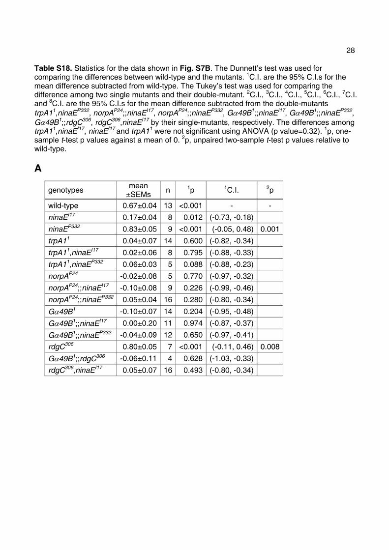
28 Table S18. Statistics for the data shown in Fig. S7B. The Dunnett’s test was used for comparing the differences between wild-type and the mutants. 1C.I. are the 95% C.I.s for the mean difference subtracted from wild-type. The Tukey’s test was used for comparing the difference among two single mutants and their double-mutant. 2C.I., 3C.I., 4C.I., 5C.I., 6C.I., 7C.I. and 8C.I. are the 95% C.I.s for the mean difference subtracted from the double-mutants trpA11,ninaEP332, norpAP24;;ninaEI17, norpAP24;;ninaEP332, G49B1;;ninaEI17, G49B1;;ninaEP332, G49B1;;rdgC306, rdgC306,ninaEI17 by their single-mutants, respectively. The differences among trpA11,ninaEI17, ninaEI17 and trpA11 were not significant using ANOVA (p value=0.32). 1p, one-sample t-test p values against a mean of 0. 2p, unpaired two-sample t-test p values relative to wild-type.

A

genotypes mean ±SEMs n 1p 1C.I. 2p

wild-type 0.67±0.04 13 <0.001 - -

ninaEI17 0.17±0.04 8 0.012 (-0.73, -0.18)

ninaEP332 0.83±0.05 9 <0.001 (-0.05, 0.48) 0.001

trpA11 0.04±0.07 14 0.600 (-0.82, -0.34)

trpA11,ninaEI17 0.02±0.06 8 0.795 (-0.88, -0.33)

trpA11,ninaEP332 0.06±0.03 5 0.088 (-0.88, -0.23)

norpAP24 -0.02±0.08 5 0.770 (-0.97, -0.32)

norpAP24;;ninaEI17 -0.10±0.08 9 0.226 (-0.99, -0.46)

norpAP24;;ninaEP332 0.05±0.04 16 0.280 (-0.80, -0.34)

G49B1 -0.10±0.07 14 0.204 (-0.95, -0.48)

G49B1;;ninaEI17 0.00±0.20 11 0.974 (-0.87, -0.37)

G49B1;;ninaEP332 -0.04±0.09 12 0.650 (-0.97, -0.41)

rdgC306 0.80±0.05 7 <0.001 (-0.11, 0.46) 0.008

G49B1;;rdgC306 -0.06±0.11 4 0.628 (-1.03, -0.33)

rdgC306,ninaEI17 0.05±0.07 16 0.493 (-0.80, -0.34)

29

B

Supplementary References 1. A. H. Brand, N. Perrimon, Development 118, 401 (1993). 2. C. S. Thummel, and Pirrotta, V., Drosoph. Inf. Serv. 71, 150 (1992). 3. Y. Kwon, H. S. Shim, X. Wang, C. Montell, Nat Neurosci 11, 871 (2008). 4. T. Washburn, J. E. O'Tousa, J. Biol. Chem. 264, 15464 (1989). 5. P. Kurada, J. E. O'Tousa, Neuron 14, 571 (1995).

genotype mean ±SEM

2C.I. 3C.I. 4C.I. 5C.I. 6C.I. 7C.I. 8C.I.

ninaEI17 0.17±0.04 (0.03, 0.50)

(-0.03, 0.36)

(-0.06, 0.29)

ninaEP332 0.83±0.05 (0.49, 1.05)

(0.61, 0.95)

(0.60, 1.15)

trpA11 0.04±0.07 (-0.29, 0.24)

trpA11,ninaEI17 0.02±0.06

trpA11,ninaEP332 0.06±0.03 -

norpAP24 -0.02±0.08 (-0.19,

0.35) (-0.29,

0.14)

norpAP24;;ninaEI17 -0.10±0.08 -

norpAP24;;ninaEP332 0.05±0.04 -

G49B1 -0.10±0.07 (-0.32, 0.13)

(-0.30, 0.19)

(-0.36, 0.29)

G49B1;;ninaEI17 0.00±0.20 -

G49B1;;ninaEP332 -0.04±0.09 -

rdgC306 0.80±0.05 (0.49,

1.21) (0.50, 0.99)

G49B1;;rdgC306 -0.06±0.11 -

rdgC306,ninaEI17 0.05±0.07 -