Age structured populations Alfred James Lotka (1880- 1949) Vito Volterra (1860-1940)

Supporting Information S2 - Lotka-Volterra food web dynamics with
moderately complex structure
Supporting Information for How do MAR(1) models cope with hidden nonlinearities in ecological dynamics?Gregoire Certain, Frederic Barraquand and Anna Gardmark, Methods in Ecology and Evolution 2018.
The associated code has DOI:10.5281/zenodo.1218024, available at https://zenodo.org/record/1218024.The corresponding GitHub repository can be browsed at https://github.com/fbarraquand/MAR_foodWeb_MEE.
1 Introduction - food web model construction
The food web dynamics has been modelled in the following manner
• A real network topology (Fig. 1) has been considered, based on the food web of Gatun lake (Aufderheideet al., 2013). It has 12 species and a connectance of 21% (27% with self-regulation terms)1. 4 species (1/3)are affected by the environmental variable.
• Based on this food web topology, parameters have been drawn at random within bounds for each simulation,for both the interaction matrix and the environmental effects.
• We used parameters maintaining feasibility of the equilibrium, i.e. strictly positive abundances for all species- as in the main text. Parameter bounds were chosen so that all simulations produce realistic time series(i.e., top predators fluctuate mildly, while r-strategists lower down the food chain can have more variabledynamics).
2 The general Lotka-Volterra-Ricker (LVR) food web model and itslog-linearized Jacobian matrix
We used a general LVR model (with environmental effects) to simulate the food web, as it allows for non-lineardynamics but maintains analytical tractability, as well as a connection to the results of the main text. The LVRmodel is written in logarithmic scale as:
nt+1 = nt + r + Cut + ANt + wt, wt ∼ MVN(0,Σ) (1)
where the vector of untransformed abundances is Nt = (N1t, ..., NSt)T = (en1t , ..., enSt)T . The matrix A = (αij)
contains all the species interaction coefficients. We assume that the kill rate of an individual predator of species jon prey from species i is βijNi. Because the dynamics are of the Lotka-Volterra predation type, we have
αij = −βij if prey i is eaten by j (2)
+εijβji if predator i eats prey j (3)
A term −βij may likewise model competitive per capita effects of species j on species i. We assume that βij = 0unless i = j. An intraspecific competition coefficient βii > 0 term combined with ri > 0 ensures logistic growth inabsence of the other species, which allows to create feasible food webs (i.e., N∗i > 0 for all i). This was especiallyimportant for the base of the food web ( see ‘Parameters’ below). Regarding the efficiency εij of predator i on
1Other choices, such as modular networks with clusters of strong interactors linked by weaker inter-cluster ties, are possible. However,they would be essentially similar to considering several interacting small modules of 2 or 3 species. The chosen food web involves somedegree of omnivory and resource competition at intermediate tropic levels, which we view as relatively common in real food webs.
1

1
23 4
5 6 7 8
9
10
11 12
Figure 1: Food web topology and interaction strength pattern (red: negative feedback, blue: positive feedback;width of arrows proportional to log(interaction strength) as indicated by J, for one randomly created parameterset)
prey j, there are different options. Setting εij = εi assumes that the predator i transforms all prey j with equalefficiency, with predators varying in their energetic conversion coefficient. εij = εj assumes on the contrary thatprey have varying energetic content, but predators have identical conversion efficiencies. Given the many choicespossible, we preferred to set εij = ε = 0.1 for simplicity.
Deriving the Jacobian matrix on a log-scale
Our model belongs to the general family of coupled nonlinear stochastic difference equations
ni,t+1 = fi((nk,t)k∈[|1,S|]
)+ εi,t (4)
where εi,t is an additive, centered Gaussian noise term. For this and similar models, the Jacobian element is
therefore Jij = ∂fi∂nj|n=n∗ . In the LVR model, we have fi(n) = ni +ci•ut +αi•Nt with αi•Nt =
∑Sk=1 αikNk,t. This
implies that
∂fi∂nj
=∂ni∂nj︸︷︷︸
=0 if i 6=j
+∂(ri + ci•ut)
∂nj︸ ︷︷ ︸=0
+
S∑k=1
αik∂enk
∂nj= δij + αije
nj (5)
with δij = 1 if i = j, and δij = 0 otherwise. Hence,
Jij = δij + αijen∗j (6)
Computation of the equilibrium point
We have at equilibrium0 = r + Cu∗ + AN∗ = r + AN∗ (7)
so thatN∗ = A−1(−r) (8)
2

We check notably the feasibility (strictly positive abundances for all species) of the equilibrium.
Interaction matrix A
Assuming there are only trophic relationships (no direct competition between species) and within-species regulation,the interaction matrix now writes
A =
−β11 0 −β31 0 0 0 0 0 0 0 0 00 −β22 0 0 0 0 0 −β28 0 0 0 0
ε31β13 0 −β33 0 −β35 −β36 0 0 0 0 0 00 0 0 −β44 −β45 −β46 −β47 0 0 0 0 00 0 ε53β35 ε54β45 −β55 0 0 0 −β59 −β5,10 −β5,11 00 0 ε63β36 ε64β46 0 −β66 0 0 0 0 0 −β6,120 0 0 ε74β47 0 0 −β77 0 0 0 0 −β7,120 ε82β28 0 0 0 0 0 −β88 0 0 0 −β8,120 0 0 0 ε95β59 0 0 0 −β99 −β9,10 0 00 0 0 0 ε10,5β5,10 0 0 0 ε10,9β9,10 −β10,10 0 00 0 0 0 ε11,5β5,11 0 0 0 0 0 −β11,11 00 0 0 0 0 ε12,6β6,12 ε12,7β7,12 ε12,8β8,12 0 0 0 −β12,12
(9)
Environmental effects
Species 1, 2, 4 and 11 were chosen to be forced (simultaneously) by the environmental variable. The idea was toforce three species at the base of the food web (to maintain a connection to the results of our main text) and alsoa species at the top of the food web.
Parameters
We chose parameter values partially at random. The mean values of intraspecific interaction strength, βintra, wasset to 0.3 for all species but species 10,11 and 12 that had βintra = 0.9. Strong regulation is indeed needed at thetop of the food web for stability. The mean interspecific interaction strength was set to 0.1. Then each interactioncoefficient was drawn as βij = δijβintra + (1− δij)βinter + Unif(−0.1, 0.1), which is then converted into αij accordingto eq. 2.
The intrinsic growth rates were different for the different trophic levels
• rpreywas 2 for species 1 and 1 for species 2 and 4.
• rintermediate ∼ Unif(0.01, 0.05). Intermediate species are assumed to reproduce very little if their prey are notpresent in the food web. We did not include negative ri (death only in absence of prey) because these had adetrimental effect on the feasibility of the food web. Also, a food web is never a complete representation ofreality, thus a negative ri does not necessarily makes sense if one thinks predator i might access at times preyoutside of the web (e.g., Erbach et al., 2013).
• rtop = 0.001 to 0.0001. The intrinsic growth rate of the top predators is considered to be very low, in linewith the fact that they need the lower trophic levels to reproduce, and their life histories are usually muchslower.
Length of the time series The number of timesteps was first set to 100, as in the two-species experiment. Thisresulted in poor, highly variable estimates including in the Gompertz model 2 (fraction of correctly detected signscloser to 0.5 than 1 for most interactions). A time series length of 800 was therefore chosen to provide an amountof data, in relation to the number of parameters estimated, that was comparable to the 2-species models of themain text. In the following, we report the results for tmax = 800. As there are intrinsically more constraints for the
2Constructing high-dimensional models for short time series typically require some procedure to “shrink” the estimates, i.e., correctfor the added variance in estimates at low sample sizes. Classical choices of regularization techniques (e.g., Basu et al., 2015) includeridge regression, the LASSO (which performs model selection at the same time), as well as some other techniques with a Bayesianperspective (e.g., Mutshinda et al., 2011; Ovaskainen et al., 2017)
3

feasibility of the equilibrium point (and the perturbed state after the PRESS) for a 12-species than 2 or 3 speciesfood web, less variation in parameter values was considered than in the 2-species simulations3.
CONTROL GOMPERTZ SIMULATION
In order to see what properties of the estimates can be attributed specifically to the LVR model, we also produceda Gompertz food web dynamics. Due to the difficulties in specifying a Gompertz food web (see Discussion in maintext), we use for B the Jacobian of the LVR model (eq. 6) with the abovementioned parameters.
3 Model fitting
We used, as in the main text, MARSS for model fitting (Holmes et al., 2014). We chose two contrasted MAR(1)model formulations, one in which the topology of the net interaction matrix was fully unknown, with a full B anda full C matrix that could take any values, and one in which it was fully known, with sparse B and C matrices,constrained by the known topology of the food web (i.e., bij was set to zero if αij was set to zero; a similar rulewas used for the environmental effect matrix C). Contrasting these two cases reveals how hidden non-linearitieschallenge the estimation of MAR models under contrasted scenarios of prior knowledge on ecological interactions.
We are aware that fitting large MAR models without long time series - and even with relatively long ones ofseveral hundred time steps - can generate massive overparameterization (Michailidis & d’Alche Buc, 2013). Forinstance, fitting a full 12-species MAR models to a 100 timepoints time series requires estimating more parametersthan time steps and require regularization techniques (e.g., Basu et al., 2015). With the 800 timesteps chosen, suchproblems remain moderate.
We fitted MAR(1) models to 100 LVR and 100 Gompertz simulations, each with randomly chosen parameterssets (as in the main text). Each time, both the MAR(1) models with the known and unknown topology were fitted,for tmax = 800. This resulted therefore in 2 × 2 × 100 = 400 MAR(1) model fits (considering only the case with800 timesteps for which we present the results below). See the GitHub/Zenodo repository for the details of thesimulation, model fitting and model comparison4. In the following, we focus on the main results of our food websimulation and model fitting experiment.
4 Results of the food web model fitting, PRESS prediction and dis-cussion
There are two complementary ways in which the estimation results (e.g., B matrix coefficients) can be presented:
1. Within-repeats summary statistics, such as the correlation between B and J of diagonal and off-diagonalelements, for one given simulation run (i.e., one repeat).
2. Across-repeats summary statistics. These include the correlation between bi,j and ji,j across repeats, as wedo in the main text, the fraction of well-recovered signs, the fraction of J elements out of 95%CIs for B.
Both within- and across-repeats statistics contain relevant information: within-repeats statistics allow to identifysimulation runs where the estimation of most elements is good or poor, while across-repeats allow to identify matrixelements that were systematically well- or poorly-estimated across simulation runs.
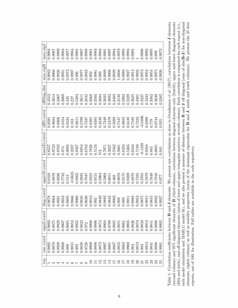
We note, however, that presenting correlations calculated using the whole B matrix for one simulation run, asdone recently by Ovaskainen et al. (2017), unfortunately tends to present an over-optimistic picture of the estimationof interpecific interactions. The correlation Cor (vec(B), vec(J)), for one repeat, is indeed often driven by a set ofpoints near (0, 0) and a set of points near (1, 1) (Fig. 2 and Table 1). We therefore recommend to at least separatediagonal from off-diagonal elements when presenting correlations (as we do below in Table 1).
INTERACTION PARAMETERS - B MATRIX
Overall, we recover the results of the main text for 2-species models:
3It may be possible to construct strongly interacting webs by allowing species extinction and a real assembly process, starting froma larger species pool. This would, however, create webs with different structure for each parameter set and impede element-by-elementcomparison, as we do here and in the main text.
4https://github.com/fbarraquand/MAR_foodWeb_MEE, version of record https://zenodo.org/record/1218024
4

−1.0 −0.5 0.0 0.5 1.0
−1.
0−
0.5
0.0
0.5
1.0
J_ij value (simulated)
B_i
val
ue (
estim
ated
)
Figure 2: Estimated vs. simulated values of B for a Gompertz simulation. The overall correlation (as reportedin Ovaskainen et al., 2017) is 98% (94% for an unknown network topology), even though the correlation betweeninterspecific elements (center cluster) is merely 50% (29% for unknown topology).
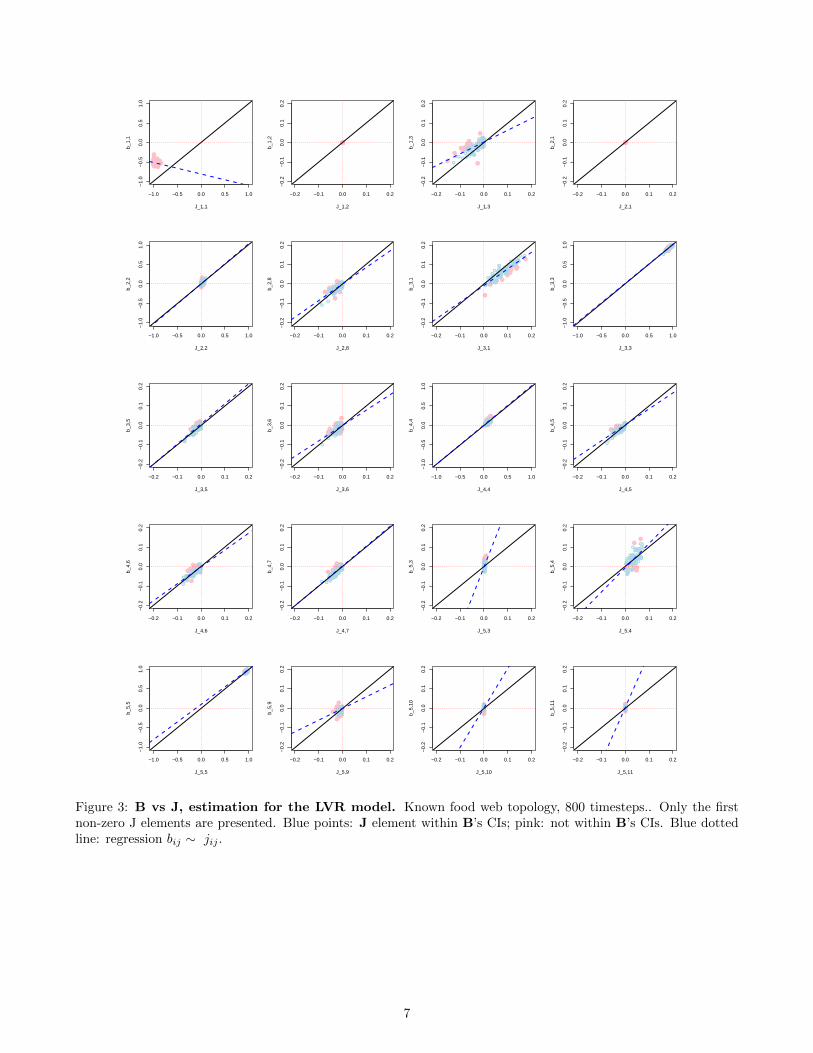
• There is a slight underestimation of interspecific interaction strengths in the LVR model (Fig. 3), as for thetwo-species LVR model MAR estimates. This is less visible than in the two-species model, because someinteraction strengths are very small and the range of variation in interaction strength is overall smaller thanin the two-species example. The underestimation is noticeable for, e.g., interactions between species 1 and 3(Fig. 3).
• The percentage of correctly identified signs across simulations is lower than in our 2-species system butstill acceptable for the lower part of the food web (78% averaged across non-zero J elements overall). Signrecovery varies quite a bit in relation to interaction strength: most reasonably strong interactions, above10−1 in absolute value, are well recovered in sign, Fig. 4. Effects of prey on predator are weaker thanthose of predator on prey, and tend to be less well recovered, especially at the top of the food web. This istrue even in the theoretical formulation of net interaction strength. We have indeed Jij = εβji exp(n∗j ) withε = 0.1 and very low n∗j for predators. The conclusion is therefore that effects prey → predator tend to beless well recovered because they are intrinsically weaker, at least when constraining our food web model toproduce lifelike species abundance distributions, with an Eltonian biomass pyramid forbidding large predatorabundances.
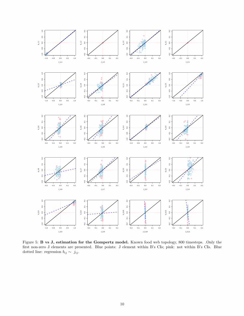
• The results are similar for a Gompertz model whose coefficients are those of the Jacobian of the LVR model.For the Gompertz case, there is less bias (underestimation) in the estimation of the B elements (which islogical) but more variance in the estimates (Fig. 5).
• The correlation between B and J off-diagonal elements for a given simulation and parameter set varies quitewidely (from 90% to negative values, Table 1). This strongly suggests that some simulations - even in theGompertz case - have poorly identified parameter combinations. These ‘bad apples’ potentially contributeheavily to the decrease in overall MAR model performance, but more work is needed to investigate the variancein estimates across parameter sets.
• Overcompensation, at least in the basal species for which the intrinsic growth rate is large (r = 2), was wellidentified. Note that species 2 and 4 have r = 1, which is at the boundary of overcompensation; therefore it
5

is normal that for those species overcompensation is less clear.
• Cases with dominant eigenvalue above 1 in norm result in a mismatch between B and J (not shown, requiresadditional parameter values), as for the LVR-T2-cycle in the main text.
• The ‘full B matrix’ model seems to identify correctly the interaction sign and strength in the Gompertz case(Fig. 6) even slightly better than the web with known topology. In the LVR case, the fraction of correctlyidentified signs for each element of interest is similar between a priori known and unknown web topologies(Table 2). Thus far, specifying the network topology has had little impact on the quality of the estimates, forthis food web simulation. Of course, there are some false positives (significant interactions at a 95% level) inB elements without constraints on B, but they seem to have moderate impact on sign recovery.
• Statistical techniques are available for regularized estimation of MAR(1) models. They would improve esti-mates of B without a knowledge of the web topology a priori (e.g., sparse modelling, dimension reductionthrough clustering; Michailidis & d’Alche Buc, 2013; Basu et al., 2015; Ovaskainen et al., 2017) and theirevaluation would need to be extended. For example, there is no evaluation in Ovaskainen et al. (2017) of in-teraction sign inference (sign is arguably key to biological interpretation), only the overall correlation betweenB elements. Unfortunately, as we show in Fig. 2, a ‘raw’ correlation between B and J elements of a singleMAR(1) model is not a reliable tool to evaluate properly the quality of off-diagonal (interspecific) coefficients.
6
●● ●●●●
●●
●
●●●●
●
●●●
●
●●
●
●
●
●
●●
●● ●●●●●●●●●●
●
●
●
●●
●
●●●●● ●●●●●●●●●
●
●●●●●
●●●
●●●
●●
●
●
●●●●●●●●●
●
●●
●●
●●●
●●●●●●
●●●
−1.0 −0.5 0.0 0.5 1.0
−1.
0−
0.5
0.0
0.5
1.0
J_1,1
b_1,
1
●●●●●●●●●●●●●●●●●●●●●●●●●●●●●●●●●●●●●●●●●●●●●●●●●●●●●●●●●●●●●●●●●●●●●●●●●●●●●●●●●●●●●●●●●●●●●●●●●●●●
−0.2 −0.1 0.0 0.1 0.2
−0.
2−
0.1
0.0
0.1
0.2
J_1,2
b_1,
2
●
●
●
●
●
●
●●
●
●●●●
●
●●●
●
●
● ●●
●
−0.2 −0.1 0.0 0.1 0.2
−0.
2−
0.1
0.0
0.1
0.2
J_1,3
b_1,
3
●●
●
●
●●●
●●●●
●
●●●
●
●
●
●
●
●●
●
●
●●
●
●●
●
● ●
●●
●
●
●
●
●●
●
●
●●● ●●
●●
●
●
●●●
●●
●●●
●●
●
●
●●●
●
●●
●
●●●●●●●●●●●●●●●●●●●●●●●●●●●●●●●●●●●●●●●●●●●●●●●●●●●●●●●●●●●●●●●●●●●●●●●●●●●●●●●●●●●●●●●●●●●●●●●●●●●●
−0.2 −0.1 0.0 0.1 0.2
−0.
2−
0.1
0.0
0.1
0.2
J_2,1
b_2,
1
●●
●●
●
●●
●
●
●
●●●●●●
−1.0 −0.5 0.0 0.5 1.0
−1.
0−
0.5
0.0
0.5
1.0
J_2,2
b_2,
2
●●●●●●●
●●●●●
●●●●●
●●●●●●●●●●●●●
●●●
●●●
●
●●●●
●●●
●●●●●●●
●●
●●●●●●●
●
●●●
●
●
●●●●●●●●●
●
●
●●●
●
●
●
●●
●●●
●●
−0.2 −0.1 0.0 0.1 0.2
−0.
2−
0.1
0.0
0.1
0.2
J_2,8
b_2,
8
●
●●●
●
●
●
●
●●
●●
●
●
●
●●
●●
●
●●●
●
●●
●●
●
●●
●
●
●●
●●●
●
●●
●
●● ●
●
●
●
●●●
●●
●
●
●●
●●
●● ●●
●●
●●
●●
●●
●●
●
●
●●
●
●
●
●
●
●
●
●
●
●
●
●
−0.2 −0.1 0.0 0.1 0.2
−0.
2−
0.1
0.0
0.1
0.2
J_3,1
b_3,
1
●● ●●
●
●
●
●
●
●
●
●
●
●●
●
●
●●
●
●
●●
●
●
●
●
●
●
●
●
●
●●
●●
●
●●●
●●
●
●
●●
●●
●
●●
●
●
●
●
●
●
●
●●● ●
●
●
●
●
●
●●
●
● ●
●
●
●
●
●
●
●
●
●
●
●
●
●●
●● ●●●●●
●●●●●●●●●●●●●
●●
●●●●●●●
−1.0 −0.5 0.0 0.5 1.0
−1.
0−
0.5
0.0
0.5
1.0
J_3,3
b_3,
3
●●
●
●
●
●
●
●●●●●●●●
●
●
●●●●●●
●
●●●
●●●●●
●●●●●
●●●●●
●●
●●●
●●●●●
●●●●●●●●●●
●●●
●●
●●●●
●
●
●●●
●●●
●●●
●
−0.2 −0.1 0.0 0.1 0.2
−0.
2−
0.1
0.0
0.1
0.2
J_3,5
b_3,
5
●●
●●●
●●●
●
●●●●●●
●●
●●●
●
●●●
●●
●●
●●
●
●●●●
●
●●●●
●●●
●
● ●●●
●
●●
●●
● ●●●
●
●
●
●●●
●●●●● ●
●
●
●
●
●●
●● ●
●
●● ●●
●
●●●●
●●
●●●
●●
●
●
−0.2 −0.1 0.0 0.1 0.2
−0.
2−
0.1
0.0
0.1
0.2
J_3,6
b_3,
6
●
●
●●●●●
●●
●
● ●●●
●
●
●
●●●
●●
●
●●
●
●●
●
●●
●
●●●●●●
●●
●
●
●●●●
●●●●●
●● ● ●●●
●
●●
●●
●
●●●
●
●●
●●
●●
●
● ●●
● ●
●●●●
●●●
−1.0 −0.5 0.0 0.5 1.0
−1.
0−
0.5
0.0
0.5
1.0
J_4,4
b_4,
4 ●●●●●●●
●●
●●●●●
●●
●●●●●
●
●●●●●●
●●
●●●
●●●●●●
●●●●●●
●●●●
●●●●●●●●●●●●●
●●●●●●
●●●●●●● ●●
●
●
●●●
●●●●●
●●●
●
●●●
●●●
●●
−0.2 −0.1 0.0 0.1 0.2
−0.
2−
0.1
0.0
0.1
0.2
J_4,5
b_4,
5
●●
●●●
●●● ●
●
●●
●
●
●●
●
●
●●
●
●
●● ●●●
●●
●
●●
●●
●
●●
●● ●
●●
●●
●
●●●
●●●●
●●
●
●●●
●●●
●●●●●●
●●
●
●
●●
●
●
●
●●●●●
●● ●
●●●
●
●●
●●
●●
●●
−0.2 −0.1 0.0 0.1 0.2
−0.
2−
0.1
0.0
0.1
0.2
J_4,6
b_4,
6
●●
●●
● ●●●
●
●
●●
●
●
●
●●●●●
●
●●●●●●
●●●
●●●●●
●● ●●●
●
●●● ●
●●
●
●
●
●●●
●●
●●●
●●
●●●●
●●
●
●● ●
●
●
●
●●
●●
●●
●●●●
●
−0.2 −0.1 0.0 0.1 0.2
−0.
2−
0.1
0.0
0.1
0.2
J_4,7
b_4,
7
●●●
●●●●
●●
●
●
●
●●●●
●
●●
●
●●
●
●●●
●●●
●
● ●
●●
●
● ●
●
●
●
●●
●●
●●
●●
●●
●
●
●●●
●●
●
●
●●
●
●●
●
●
●
●
●
●
●●
●
●●●
●●
●●
●
●
●●●
●
●
●●●
●
●
●
●
−0.2 −0.1 0.0 0.1 0.2
−0.
2−
0.1
0.0
0.1
0.2
J_5,3
b_5,
3
●
●
●
●
●●●●●●●
●
●●●
●
●●●●●
●●
●
●
●●●●●
●●
●●●
●
●
●●●
●●
●●
●
●
●●●●●●●●●●●
●●●
●●●
●
●
●
●●
●●
●●
−0.2 −0.1 0.0 0.1 0.2
−0.
2−
0.1
0.0
0.1
0.2
J_5,4
b_5,
4●●
●
●●
●
●
●●
●
●●● ●●
●
●
●
●
●
●
●
●●●● ●●
●
●
●●●
●
●
●●
●
●
●
●
●
● ●
●
●
●●
●
●●
●
●
●●●
●
●●
●
●
●
●●
●
●● ●● ●
●●
●●
●
●
●
●
●●●●●●●
●●●●●●●●●●●●●●●●●●
●
−1.0 −0.5 0.0 0.5 1.0
−1.
0−
0.5
0.0
0.5
1.0
J_5,5
b_5,
5
●●●●●●●●●●●
●●●●●●●●
●●●●●●●●●●
●●●●
●●●●●●●●●●●●
●●●●●●
●●●●●●●●●
●●
●●
●●●●●●●●●
●
●
●
●●●
●
●
●
●
●●
●●●●●
−0.2 −0.1 0.0 0.1 0.2
−0.
2−
0.1
0.0
0.1
0.2
J_5,9
b_5,
9
●●●
●●
●●●●●●●
●●●●●●●●●●●●●●●●●●●
●●●●
●
●
●●●●●
●
●●●●●●●●●●●●●●
●●
●●
●●
●●
●
●●●
●
●●●●●
●
●
●●●●●
●●
−0.2 −0.1 0.0 0.1 0.2
−0.
2−
0.1
0.0
0.1
0.2
J_5,10
b_5,
10
●●●●●●●
●●●●●●●●●●●●●●●●●●●●●●●●●●●●●●●●●●●●●●●●●●●●●●●●●●●
●●●●●●●●●●●●●
●●●●●●
●
●●●●●
−0.2 −0.1 0.0 0.1 0.2
−0.
2−
0.1
0.0
0.1
0.2
J_5,11
b_5,
11
●●●●●●●●●●●●●●●●●●●●●●●●●●●●●●●●●●●●●●●●●●●●●●●●●●●●●●●●●●●●●●●●●●●●●●●
Figure 3: B vs J, estimation for the LVR model. Known food web topology, 800 timesteps.. Only the firstnon-zero J elements are presented. Blue points: J element within B’s CIs; pink: not within B’s CIs. Blue dottedline: regression bij ∼ jij .
7

●
●
●
●
●
●
●●
●
●●
●
●
●
●
●
●●
●
●
●
●
●
●
●
●
●
●
●
●
●
●●
●
●
●
●
●
●
●
−3.5 −3.0 −2.5 −2.0 −1.5 −1.0 −0.5 0.0
0.5
0.6
0.7
0.8
0.9
1.0
log(|Interaction Strength|)
Fra
ctio
n of
cor
rect
inte
ract
ion
sign
s
Figure 4: Relationship between the fraction of correctly identified interaction signs and the log(interaction strength).
8
rep.
raw
corr
elsi
gnif
corr
eldia
gco
rrel
up
per
Dco
rrel
low
erD
corr
eloff
Dco
rrel
off
Dia
gdis
tm
ax
eigB
max
eigJ
10.
9895
0.98
930.
9878
0.8
104
0.8
557
0.8
281
0.4
313
0.9
943
0.9
994
20.
9879
0.98
750.
9904
0.9
876
0.9
723
0.9
684
0.2
614
0.9
966
0.9
987
30.
9929
0.99
290.
9921
0.9
596
0.8
702
0.8
906
0.3
367
0.9
926
0.9
999
40.
9908
0.99
070.
9924
0.7
732
0.8
74
0.8
454
0.2
669
0.9
931
0.9
984
50.
989
0.98
850.
9895
0.5
13
0.9
095
0.8
234
0.4
35
0.9
972
0.9
977
60.
9851
0.98
530.
9866
-0.0
625
0.2
027
0.1
83
0.2
27
0.9
997
0.9
984
70.
993
0.99
350.
9966
0.8
862
0.8
567
0.8
611
0.5
384
0.9
96
0.9
985
80.
9828
0.98
230.
9835
0.3
935
0.6
954
0.5
799
0.3
611
0.9
977
0.9
987
90.
9726
0.97
20.
9636
0.7
947
0.6
782
0.7
337
0.2
842
0.9
942
0.9
998
100.
9909
0.99
080.
9913
0.9
255
0.7
828
0.8
391
0.2
868
0.9
92
0.9
991
110.
9898
0.98
960.
992
0.9
151
0.5
124
0.6
385
0.3
503
0.9
981
0.9
983
120.
9873
0.98
740.
9849
0.5
964
NA
0.3
249
0.3
884
0.9
99
0.9
988
130.
9907
0.99
040.
9892
0.5
968
0.7
971
0.7
349
0.3
023
0.9
949
0.9
991
140.
9801
0.97
990.
9842
0.0
011
0.3
027
0.2
479
0.3
892
0.9
966
0.9
997
150.
9887
0.98
850.
9902
0.4
68
0.5
562
0.5
089
0.3
483
0.9
929
0.9
984
160.
9855
0.98
510.
989
0.9
078
0.5
661
0.7
447
0.3
138
1.0
008
0.9
979
170.
9862
0.98
610.
989
0.9
175
0.8
334
0.8
682
0.2
962
0.9
988
0.9
995
180.
9908
0.99
050.
9911
0.8
209
0.5
365
0.6
448
0.2
329
0.9
927
0.9
994
190.
984
0.98
360.
9868
0.8
878
0.6
344
0.7
188
0.3
625
0.9
914
0.9
995
200.
9873
0.98
730.
9953
0.7
585
0.7
189
0.7
222
0.4
301
0.9
902
121
0.98
30.
9833
0.98
75
0.3
765
-0.1
329
-0.0
496
0.3
227
0.9
973
0.9
998
220.
9913
0.99
130.
9915
0.5
879
0.9
358
0.8
398
0.3
433
0.9
954
0.9
992
230.
9841
0.98
410.
9855
0.7
648
0.8
85
0.7
78
0.3
562
0.9
955
0.9
995
240.
9898
0.98
980.
9932
0.7
816
0.6
881
0.6
744
0.3
649
0.9
975
0.9
99
250.
9901
0.99
020.
9927
0.9
77
0.9
41
0.9
55
0.3
382
0.9
926
0.9
972
Tab
le1:
Cor
rela
tion
coeffi
cien
tsb
etw
een
Ban
dJ
elem
ents
.W
epre
sent
raw
corr
elati
on
sas
don
ein
Ova
skain
enet
al.
(2017),
corr
elati
ons
bet
wee
nJ
elem
ents
(sec
ond
colu
mn)
and
95%
sign
ifica
nt
elem
ents
ofB
(th
ird
colu
mn
),co
rrel
ati
on
bet
wee
nd
iagonal
elem
ents
on
ly(f
ou
rth
),up
per
and
low
erdia
gon
al
elem
ents
(fift
han
dsi
xth
),an
doff
-dia
gonal
elem
ents
(un
ion
oflo
wer
an
du
pp
ertr
iangula
rm
atr
ices
,se
venth
colu
mn
).E
ach
corr
elati
on
isco
mpu
ted
for
each
rep
eat
(i.e
.,ea
chm
od
elsi
mula
tion
and
MA
R(1
)m
odel
fit)
,an
dw
eals
opre
sent
am
easu
reof
dis
tance
bet
wee
nB
and
Joff
dia
gon
al
(sum
of
abs(
B-J
)fo
rnon
-dia
gonal
elem
ents
,ei
ghth
colu
mn)
asw
ell
asst
abilit
ypro
per
ties
(norm
of
the
dom
inant
eigen
valu
efo
rB
and
J,
nin
than
dte
nth
colu
mns)
.W
epre
sent
the
25
firs
tre
pea
ts,
out
of10
0,fo
rillu
stra
tion
.F
ull
tab
les
are
available
inth
eco
de
rep
osi
tory
.
9
●●●●
−1.0 −0.5 0.0 0.5 1.0
−1.
0−
0.5
0.0
0.5
1.0
J_1,1
b_1,
1
●●●
●●●●
●●
●●●
●
●●●●●
●●
●
●●●●●●●●●●●●●●
●●●●●●●●
●
●
●●●●●●●●●●●●●●●●
●●●●●●●
●●●
●●
●●●●●●●●●●●●●●●●●●
●●●
●●
●●●●●●●●●●●●●●●●●●●●●●●●●●●●●●●●●●●●●●●●●●●●●●●●●●●●●●●●●●●●●●●●●●●●●●●●●●●●●●●●●●●●●●●●●●●●●●●●●●●●
−0.2 −0.1 0.0 0.1 0.2
−0.
2−
0.1
0.0
0.1
0.2
J_1,2
b_1,
2 ●
●
−0.2 −0.1 0.0 0.1 0.2
−0.
2−
0.1
0.0
0.1
0.2
J_1,3
b_1,
3 ●
●
●
●
●
●
●
●
●
●
●
●
●
●
●
●
●
●●
●
●
●●
●●
●
●●
●●
●
●
●
●
●
●
●
●
●●
●
●
●
●
●
●
●
●
●●
●
●
●
●
●
●
●
●
●
●
●
●
●●
●
●
●
●
●
●
●
●●
●
●
●
●●
●
●
●
●
●●
●
●
●
●
●●
●●●
●●
● ●
●
●●●●●●●●●●●●●●●●●●●●●●●●●●●●●●●●●●●●●●●●●●●●●●●●●●●●●●●●●●●●●●●●●●●●●●●●●●●●●●●●●●●●●●●●●●●●●●●●●●●●
−0.2 −0.1 0.0 0.1 0.2
−0.
2−
0.1
0.0
0.1
0.2
J_2,1
b_2,
1
●
●
●
●
●
−1.0 −0.5 0.0 0.5 1.0
−1.
0−
0.5
0.0
0.5
1.0
J_2,2
b_2,
2
●
●●●
●●
●
●●
●
●●●●
●●●●
●●●
●●
●
●
●
●●
●●●●
●●●●●
●
●
●
●●●●●●
●●
●
●
●
●
●
●●●●●●●●●
●●●
●●●
●●●
●
●
●
●
●
●●●
●
●●
●●●
●
●
●●
●●●
●●
●
●
●
●●
●
●
●
−0.2 −0.1 0.0 0.1 0.2
−0.
2−
0.1
0.0
0.1
0.2
J_2,8
b_2,
8
●
●
●
●●
●●
●
●
●
●
●
●
●
●
●
●● ●
●
● ●●●●
●
●●
●●
●●
●●
●●
●
●●● ●
●●
●
●
●●
●
●●
●●
●
●●
●
●
●
●
●● ●●
●●
●●
●
●
●●
●
●
●
●
●
●●
●
●
●
●
●
●
●
●
●
●
●●
●
●●
●
●●
●
−0.2 −0.1 0.0 0.1 0.2
−0.
2−
0.1
0.0
0.1
0.2
J_3,1
b_3,
1
●
●
●
●
●
●
●
● ●
●
●
●
●
●
●
●
●
●
●
●
●
●
● ●
●
●
●
●
●
●
●●
●
●
●
●●
●
●
●●
●
●
●●
●
●●
●
●
●
●
●
●
●
●
●●
●
●
●
●
●●
●
●
●
●●
●
●
●
●●
●
●
●●
●
●
●
●
●
●●
●
●
●
●
●
●
●
●
●●
●
●
●●●
●●
●
●●
●●●
●
●
●
●
●●
●●
●
●
−1.0 −0.5 0.0 0.5 1.0
−1.
0−
0.5
0.0
0.5
1.0
J_3,3
b_3,
3
●●●
●● ●●●
●●●●
●●●
●
●
●
●●●●●●
●●
●●●●●●●●●●
●
● ●● ●●●
●●
●
●●●
●
●●●
●● ●●●●
●●●●
●●●●
●●●●●
●●●
●
●
●●
●
●
●
●
●
●
●●
●
−0.2 −0.1 0.0 0.1 0.2
−0.
2−
0.1
0.0
0.1
0.2
J_3,5
b_3,
5 ●●
●
●
●
●
●
●●
●
●
●
●
●●
●●
●●
●
●
●●
●
●
●
●
●●
●
●
●
●
●
●
● ●
●
●
●
●●●
●
●
●●
●
●
●
●
●
●
●
●
●
●
●
●
●
●●
●
●
●
●●
●
●
●
●
●
●
●
●
●
●
●●
●
●
●●
●●
●
●
●
● ●
●
●
●
●
●●
●
−0.2 −0.1 0.0 0.1 0.2
−0.
2−
0.1
0.0
0.1
0.2
J_3,6
b_3,
6
●
●
●
●●
●
●
●
●●●
●●
●
●
●
●
●
●● ●
●
●
●
●
●
●●
●
●
●
●●
●
●
●
●
●●
●●
●
●
●
●
●
●
●
●
●
●
●
●
●
●
●
●
●●
●
●
●
●●
●
●
●
●
●
●
● ●
●
●
●
●●
●
●
●
●
●
●
●
●
●
●
●●●●
●●●
−1.0 −0.5 0.0 0.5 1.0
−1.
0−
0.5
0.0
0.5
1.0
J_4,4
b_4,
4 ●●
●●●●
●●
●
●
●
●●●
●●●●
●●
●
●
●
●●●
●●
●●●●
●
●●
●●●●
●●●●
●●●●
●
●●●
●●●●
●●
●
●●
●●
●●●
●●
●●●●
●●
●●
●●●●
●
●●
●
●●●
●
●
●
●
●
●
●
●
●
●●
−0.2 −0.1 0.0 0.1 0.2
−0.
2−
0.1
0.0
0.1
0.2
J_4,5
b_4,
5
●
●●
●●
●
●
●●●
●
●
●
●
●
●
●●●●
●
●●
●
●●
●
●●●
●
●
●
●
●●
●
●
●●
●●
●
●
●
●
●
●
●
●●●
●
●
●
●
●
●
●
●
●
●
●
●
●
●
●
●
●●
●●
●
●
● ●
●
●
●
●
●
●
●
●●
●
●
●
●
●
●●
●
●
−0.2 −0.1 0.0 0.1 0.2
−0.
2−
0.1
0.0
0.1
0.2
J_4,6
b_4,
6
●●
●
●
●●
●
●
●
●
●
●
●
●
●
●
●
●
●
●
●●
●
●
●
●
●
●●
●●
●●
●
●●
●
●
●●
●
●
●
●●
●
●
●
●
●
●
●
●
●
●●●
●
●●
●
●
●
●
●
●
●
●
●
●
●
●●
●
●
●●
●
●
●
●
●
●
●
●
●●
●●
●
●
●
●
●
●
●
●●
●
●
●
●
●
●
●
●
−0.2 −0.1 0.0 0.1 0.2
−0.
2−
0.1
0.0
0.1
0.2
J_4,7
b_4,
7
●
●
●
●
●
●
●
●
●●
●
●●●●
●●
●
●
●
●●
●
●
●
●
●
●
●
●●
●●
●
●
●
●●
● ●
●
●
●
●●
●
●
●
●
● ●●
●
●
●
●
●
●
●
●
●
●
●
●
●
●
●●
●
●
●
●
●
●●
●●
●
●
●
●●
●●●
●
●
●
●
●●
●
●
●
●
●●
●
−0.2 −0.1 0.0 0.1 0.2
−0.
2−
0.1
0.0
0.1
0.2
J_5,3
b_5,
3
●
●
●
●
●●
●
●●
●
●
●
●
●●
●
●
●
●
●
●
●●
●
●
●
●
●●
●
●
●
●
●●
●
●
●
●●●
●
●
●
●
●
●
●●
●
●
●●
●
●
●●
●
●●
●
●
●●
●●
●
●●●
●●●●●
●
●
●
●
●●
●
●
●●
●
●
●
●
−0.2 −0.1 0.0 0.1 0.2
−0.
2−
0.1
0.0
0.1
0.2
J_5,4
b_5,
4
●
●
●●
●
●
●
●
●
●
●
●
●
●●
●
●
●
●
● ●
●
●
●
●
●
●
●
●●●
●
●
●
●
●
●
●
●
●
●
●
●
●
●
●
●
●
●
●
●
●
●
●
●
●
●
●
●
●
●
●
●
●
●
●
●●
●●
●
●
●
●
●
●
●
●
●●●
●
●
●
●
●
●
●
●
●
●
●
●●●
●
●●●
●●●
●
●●●
●
●●●●●
●
●
●
●●
●●●●
●
●●●
●●
●
●●●●
●●●●
●●●●●
−1.0 −0.5 0.0 0.5 1.0
−1.
0−
0.5
0.0
0.5
1.0
J_5,5
b_5,
5
●●
●●
●
●●●●●●●●●●
●●
●●
●
●
●●●●●●●●●●●●
●●●
●
●●●●●●●●●●
●●●●
●
●
●
●
●
●
●
●
●
●
●
●
●
−0.2 −0.1 0.0 0.1 0.2
−0.
2−
0.1
0.0
0.1
0.2
J_5,9
b_5,
9
●
●
●
●
●
●
●
●
●
●
●
●
●
●
● ●
●
●
●
●
●
●
● ●
●●●
●●
●
●
●
●
●
●
●●
●
●
●●
●
●
●
●
●
●
●
●
●
●
●
●
●
●
●
●
●
●
●
●●
●
●
●
●
●
●
●
●
●
●
●
●
●
●●
●
●●
●
●●
●
●
●
●
●
●
●
●
●
●
●
●
●
●
●
●
●
●
●
●
●
●
●
●
−0.2 −0.1 0.0 0.1 0.2
−0.
2−
0.1
0.0
0.1
0.2
J_5,10
b_5,
10 ●
●
●●
●
●
●
●
●
●
●
●●●
●●
●
●●
●
●
●
●
●
●
●
●
●
●
●
●●
●
●
●
●
●
●
●
●
●
●
●
●
●
●
●
●
●●
●
●
●
●
●
●●
●
●
●
●
●●
●
●
●
●●●●●
●●
●●
●●
●
●●●
●
●
●●
●
●
●
●
●
●
−0.2 −0.1 0.0 0.1 0.2
−0.
2−
0.1
0.0
0.1
0.2
J_5,11
b_5,
11
●
●
●
●
●
●
●
●●●●
●
●
●
●
●
●
●
●
●
●
●
●
●
●
●
●
●
●
●
●●
●
●
●
●
●
●
●●
●
●
●
●
●●
●
●
●
●
●●
●
●
●
●
●
●●
●
●●●●
●
●
●
●●
●
●
●
●●
●
●
●
●
●●
●
●●●
Figure 5: B vs J, estimation for the Gompertz model. Known food web topology, 800 timesteps. .Only thefirst non-zero J elements are presented. Blue points: J element within B’s CIs; pink: not within B’s CIs. Bluedotted line: regression bij ∼ jij .
10

●
−1.0 −0.5 0.0 0.5 1.0
−1.
0−
0.5
0.0
0.5
1.0
J_1,1
b_1,
1
●●●●
●●
●●●●
●●●●
●●●●●●
●●●●●●●●●●●●●●●●
●●●●●●●●●
●●
●
●●●●●●●●
●●●●●●●●●●●●●●●
●●●●
●●●●●●●●●●●●●●●●●●●●●●
●●
●●●
−0.2 −0.1 0.0 0.1 0.2
−0.
2−
0.1
0.0
0.1
0.2
J_1,2
b_1,
2
●●
●
●
●
●
●
●
●
●
●●
●
●●
●
●
●
●
●
●
●
●●●
●●
●
●
●●●
●
●
●●
●●
●
●
●
●
●
●
●
●
●
●●
●
●
●
●
●●
●●●
●
●
●
●
●
●
●
●
●●●
●●
●
●●●
●
●
●●
●●
−0.2 −0.1 0.0 0.1 0.2
−0.
2−
0.1
0.0
0.1
0.2
J_1,3
b_1,
3
●
●
●
●●
●
●
●
●
●
●
●
●
●
●
●
●
●
●●●
●
●●●
●
●●
●
●●●
●
●
●●
●
●
●
●
●
●●
●●
●●
● ●●
●●
●
●●●
●●●
●
●
●
●●
●●●
●●
●●●
●●
●
●
●●
●●
●●
●●
●
●
●●●●
−0.2 −0.1 0.0 0.1 0.2
−0.
2−
0.1
0.0
0.1
0.2
J_2,1
b_2,
1
●●●●●●●
●●●●●
●●●●●●●●●●●●●●●●●●●●●●●●●●●●●●●●●●●●●●●●●●●●●●●●●●●●●●●●●●●●●●●●●
●●●●
●●●●●●●
●●●●●
−1.0 −0.5 0.0 0.5 1.0
−1.
0−
0.5
0.0
0.5
1.0
J_2,2
b_2,
2
●●●●●
●●●●●●
●●●●●●●●●●●●●●●
●●●●●●
●●
●●●●●●●●●
●●●●●●●●●
●●●●●●●●●●●●●●
●●●●●●●●
●
●
●●●
●
●
●
●
−0.2 −0.1 0.0 0.1 0.2
−0.
2−
0.1
0.0
0.1
0.2
J_2,8
b_2,
8
●
●
●
●
●●
●
●
●
●●● ●
●
●●
●●
●
●
●
●●
●
●●●
●●
●
●
●
●
●●
●●● ●
●●
●
●●●
●
●
●●●
● ●●●
●●
●
●
●
●
●
●●
●
●●●
●●
●
●●
●
●●
●●
●●
●
●
●
●●
●●
●
●●
●
−0.2 −0.1 0.0 0.1 0.2
−0.
2−
0.1
0.0
0.1
0.2
J_3,1
b_3,
1
●
● ●
●
●
●
●
●
●
●
●
●
●
●●● ●
●
●
●
●
●
●
●●
●
●
●
●
●●
●
●
●
●
●
●●
●
●●
●●●
●
●
●
●
●
●●●
●
●
●
●●●
●●
●
●
●
●●
●
●
●
●
●
●
●
●
●
●●
●
●
●●
●●
●
●
●
●●
●●
●●●
●
●
●●●
●●
●●●
●●●●
●●●
●●●●●
●●●●●●●
−1.0 −0.5 0.0 0.5 1.0
−1.
0−
0.5
0.0
0.5
1.0
J_3,3
b_3,
3
●●●●
●
●●
●●
●●●
●●●●
●●●●
●●●●
●●●●●●●●●●●
●
●
●●●●
●●
●●●●●●
●●●●
●●●●●●●
●●●●●●●●●●
●●●
●●●
●●
●
●
●●
●
●●
●
●
●●
−0.2 −0.1 0.0 0.1 0.2
−0.
2−
0.1
0.0
0.1
0.2
J_3,5
b_3,
5
●●●●●●
●
●●
●
●
●
●
●
●●●
●●
●●●●●●●
●
●
●
●
●●
●
●●
●●
●
●●●
●●● ●●●●
●
●●●●●
●
●
●●
●
●
●
●●
● ●●
●●
●
●
● ●●●
●
●
●
●●●
●●●
●
−0.2 −0.1 0.0 0.1 0.2
−0.
2−
0.1
0.0
0.1
0.2
J_3,6
b_3,
6
● ●
●●
●●
●
●●
●
●●●
●
●
●
●
●
●●
●
●
●
●
●
●●
●● ●
● ●●
●●
●
●
●
●
●●●
●●●
●●
●
●●●
●●●
●●
●●●
●●●●●
●●
●●
●●●●●
●●● ●
●
● ●●●
● ●●●●●●
−1.0 −0.5 0.0 0.5 1.0
−1.
0−
0.5
0.0
0.5
1.0
J_4,4
b_4,
4 ●●●●●●●●●●●
●●●●●
●●●●●
●●●●●●●
●●●●●●●
●●●●●
●●●●●●●●●●●●●●
●●●●●●
●●●●
●●●●●●
●●●●●●●●
●●●●
●●●●●●
●●
●●
●
●●
−0.2 −0.1 0.0 0.1 0.2
−0.
2−
0.1
0.0
0.1
0.2
J_4,5
b_4,
5
●
●●
●
●●
●
●
●●
●
●
●
●
●●
●
●●●
●●●●
●
●●●
●●
●
●
●●
●●
●●
●
●
●● ●
●●
●●
●
●
●
●
●
● ●●●
●●
●●
●
●
●●
●
●
●
●●
●●
●
●
●
●●
●
●●
●
●●
●
●
●
●
●
−0.2 −0.1 0.0 0.1 0.2
−0.
2−
0.1
0.0
0.1
0.2
J_4,6
b_4,
6
●
●
●
●
●●
●●●
●
●●
●
●●●●
●●●●
●●
●
●
●● ●
●
●
●
●
●
●
●
●
●
●
●
●
●
●●●● ●
●●
●
●●
●
●
●
●
●● ●●
●●
●
●●●●
●
●
●
●
●●
●
●●
●
●●●
●●
●●
●
−0.2 −0.1 0.0 0.1 0.2
−0.
2−
0.1
0.0
0.1
0.2
J_4,7
b_4,
7
●
●
●
●● ●●●
●
●●
●● ●●●
●
●●
●
●●
●●●
●● ●
●
●● ●
●
●
●●●
●
●●●
●●
●
●●●●●
●
●
●
●●●
●●
●
●●●●●
●●
●●●
●●●●
●
●● ●●●
●
●●
●
●●
●●●
●
●
●●
●
●
●
●
−0.2 −0.1 0.0 0.1 0.2
−0.
2−
0.1
0.0
0.1
0.2
J_5,3
b_5,
3
●●
●
●
●
●
●●
●
●
●●●●●
●●
●
●●●
●●●●●
●
●●●
●●
●●
●
●●●
●●
●
●●●●
●●●
●●
●●●●●
●●
●
●●●●●●●●
●
●●
●
●
●
●
●
●
●
●
●
●
●
●
−0.2 −0.1 0.0 0.1 0.2
−0.
2−
0.1
0.0
0.1
0.2
J_5,4
b_5,
4
●
●
●
●●●
●●
●
●
●
●
●
●
●
●
●
●
●
●
●
●
●
●●
●
●
●●
●
●
● ●●
●
●●
● ●●
●
●
●
●
●
●
●
●
●
●
●
●●●
●●
● ●
●
●●
●●●
●●
●●
●●
●●
●●
●●●
●●●●●●●●●
●●●●●●●●●
●●●●
●●●
−1.0 −0.5 0.0 0.5 1.0
−1.
0−
0.5
0.0
0.5
1.0
J_5,5
b_5,
5
●●●●●●●
●●
●●●
●●●●●●●●●
●●●●●●●
●●●●●●●●●●●
●●
●●●●●●●●●●
●●●●●●●●●●●●●●●●●●●
●
●
●●
●
●●●●●●●
●
−0.2 −0.1 0.0 0.1 0.2
−0.
2−
0.1
0.0
0.1
0.2
J_5,9
b_5,
9
●●
●●
●
●
●
●●●
●
●
●
● ●
●
●●
●
●
●●●●
● ●●●●●●
●
●●● ●
●●● ●●●
●●
●●
●●
●●●●●●
●●
●●●●
●
●●
●●●●●●●●
●●
●
●●●
●
●●●
●●
●
●●●●
●●
−0.2 −0.1 0.0 0.1 0.2
−0.
2−
0.1
0.0
0.1
0.2
J_5,10
b_5,
10
●●●●●●●●●●●●●●●●●●●●●●●●●●●●●●●●●●●●●●●●●●●●●●●●●●●●●●●●●●●●●●●●
●
●●
●
●
●
●●●
●●●●
−0.2 −0.1 0.0 0.1 0.2
−0.
2−
0.1
0.0
0.1
0.2
J_5,11
b_5,
11
●●●●●●●●●●
●●●●●●●●●●●●●●●●●●●●●●●●●●●●●●●●●●●●●●●●●●●●●●●●●●●●●●●●●●
Figure 6: B vs J, estimation for the Gompertz model. Unknown food web topology, 800 timesteps.
11

●● ●●●●
●●
●
●●●●
●
●●●
●
●●
●
●
●
●●
●●● ●●●●●●●●●●
●
●
●
●●
●
●●●●● ●●●
●●●●●●
●
●●●●●
●●●
●●●
●●
●
●
●●●●●●●●●
●
●●
●●
●●●●●●●
●●●●●
−1.0 −0.5 0.0 0.5 1.0
−1.
0−
0.5
0.0
0.5
1.0
J_1,1
b_1,
1
●
●
●
●
●
●
●
●
●
●
●
●
●
●
●
●
●
●
−0.2 −0.1 0.0 0.1 0.2
−0.
2−
0.1
0.0
0.1
0.2
J_1,2
b_1,
2
●●●
●
●●●
●
●
●
●
●
●
●●●
●
●
●
●
●
●
●
●
●●
●
●●
●
●●
●●●
●
●
●
●
●
●
●
●
●
●
●
●
●
●●●●
●
●
●
●
●
●
●
●●
●●●
●
●
●
●
●
●
●
●
●
●
●
●
●● ●●
●●
● ●●
●
−0.2 −0.1 0.0 0.1 0.2
−0.
2−
0.1
0.0
0.1
0.2
J_1,3
b_1,
3
●
●
●
●
●
●
●
●
●●
●
●●
●
●
●
●
●
●●
●
●
●
●
●
●
●●
●
●●●
●
●
●
●
●
●
● ●
● ●
●●
●
●●
●●
●
●
●
●
●
●
●●
●
●
●●
●
−0.2 −0.1 0.0 0.1 0.2
−0.
2−
0.1
0.0
0.1
0.2
J_2,1
b_2,
1
●●
●
●
●●
●
●
●
●
●●●
●●●●
●
●●
●
●●●●●
●
●
●
●●
●
●
●
●
●●●
●●●●
●
●
●
●
●●●●●
●
●●●●●
●
●●●●
●
●●●●●
●
●●
●●
●●
●
●●●
●●
●
●●
●
●
●●●●●●●
−1.0 −0.5 0.0 0.5 1.0
−1.
0−
0.5
0.0
0.5
1.0
J_2,2
b_2,
2
●●●●●●
●●●●●●●●●
●●●●●●●●●●●●●●●●●●●●●
●●●
●
●●
●●●●●●●
●●●●
●
●●●●●●●● ●●
●●
●
●
●●
●●
●
●
●
●
●● ●
●
−0.2 −0.1 0.0 0.1 0.2
−0.
2−
0.1
0.0
0.1
0.2
J_2,8
b_2,
8
●
●
●●●
●●
●●●
●●●●
●
●
●
●
●
●●●
●
●
●
●● ●●●●●
●●●
●
●●
●●●
●●
●●
●●
● ●●
●
●●●●
●
●●
●
●●
●●●
●
●
●●
●●
●
●
●
●
●
●●
●
●
●
●
●●
●
●
●
−0.2 −0.1 0.0 0.1 0.2
−0.
2−
0.1
0.0
0.1
0.2
J_3,1
b_3,
1
●● ●●
●
●
●
●
●
●●
●●
●
●
●
●●●
●
●●
●●
●
●
●
●
●
●
●●
●
●
●●●
●●
●
●
●●
● ●
●
●●
●
●
●
●
●
●
●
●●● ●●
●
●●
●
●● ●
●
●
●
●
●
●
●
●
●
●
●
●●
●●●
●●
●●●●● ●● ●
●
●●●● ●
●●
●●
●
● ●
●
●●●
●●●●●
●●●●
−1.0 −0.5 0.0 0.5 1.0
−1.
0−
0.5
0.0
0.5
1.0
J_3,3
b_3,
3
●●
●
●●●●●
●
●
●●
●
●●●●●
●
●●●●
●●●●●
●●●●●
●●●
●●●
●●●●●●●
●●●
●●●●●●
●●●
●●●
●● ●
●● ●●
●●
−0.2 −0.1 0.0 0.1 0.2
−0.
2−
0.1
0.0
0.1
0.2
J_3,5
b_3,
5
●●
●●●●●
●●
●●●●
●●
●
● ●●
●
●●
●
●
●
●●●
●●●
●●
●
●●
●●
●
●●
● ●●●
●
●● ●
●●●● ●
●
●
●
●● ●● ●
●
●
●●●●
●
●●
●
● ●●●
●●
●
●
●●
●
●
−0.2 −0.1 0.0 0.1 0.2
−0.
2−
0.1
0.0
0.1
0.2
J_3,6
b_3,
6
●●●●
●
●
●●
●●
●●
●
●●
●
●
●
●
●
●
●
●
●
●
●●
●●
● ●●●
●●
●●
●
●●
●●
●●●●● ●●●
●●
●●●
●●●
● ●●
●●
●
●●
● ●●
●
●●●
●
●●
●
●
−1.0 −0.5 0.0 0.5 1.0
−1.
0−
0.5
0.0
0.5
1.0
J_4,4
b_4,
4 ●●●●●●●●
●●●
●●●
●●●●●●
●
●●●●●●●
●●
●●
●
●●●●
●●●●●●
●●●●
●●●●●●●●●●●●
●●●●●●●
●●●●● ●●
●
●
●●●
●●●●
●●
●●●●
●●
●●
●
−0.2 −0.1 0.0 0.1 0.2
−0.
2−
0.1
0.0
0.1
0.2
J_4,5
b_4,
5
●●
●● ●●● ●●
●
●●
●●
●
●
●●●
●●● ●
●●●
●●●
●
●●
●
●●
●●
●●
●
●●
●●
●●●
●●●●
●
●
●●●
●
●●
●●●
● ●
●
●●
●
●●●
●●
●
● ●●
●●
●
●●●
●
●●●●
●●
●●
−0.2 −0.1 0.0 0.1 0.2
−0.
2−
0.1
0.0
0.1
0.2
J_4,6
b_4,
6
●●
●●●● ●
●
●
●
●●
●●●
●●
●●●●
●●
●●●
●●
●
●●
●●
●● ●
●●●
●
●●● ●
●●
●
●
●
●●●●
● ●
●
●
●●●
●●
●
●●
●
●
●
●
●
●
●●
●
●
●●●
●●●
●●
●
−0.2 −0.1 0.0 0.1 0.2
−0.
2−
0.1
0.0
0.1
0.2
J_4,7
b_4,
7
●●
●●●●●
●
●●●●●
●●
●
●●
●
●●●
●
●●●
●
●
●●
●
● ●
●
●
●
●●
●
●●
●●●
●●
●
●
●
●●
●●●
●
●
●
●
●
●●
●
●
●●
●●
●
●
●
●●
●
●
●●
●
●
●●●●
●
●
●
●
●
●
●
●
●●
●
●
−0.2 −0.1 0.0 0.1 0.2
−0.
2−
0.1
0.0
0.1
0.2
J_5,3
b_5,
3
●●●
●
●
●●●●
●
●
●●●
●●●
●
●●
●●
●
●●●●●●●●●
●●
●●
●
●●●
●
●
●●
●
●●
●●●●●●●●●●●
●
●●
●
●●
●
●●
●●
●●●
−0.2 −0.1 0.0 0.1 0.2
−0.
2−
0.1
0.0
0.1
0.2
J_5,4
b_5,
4●●
●
●●
●
●●
●
●
●● ●
●
●
●
●●
●
●
●
●
●
●
●
●
● ●●
●
●●
●
●
●
●
●
●
●
●
●
●
● ●
●
●
●●
●
●●●●●
●
●
●
●
●●
●
●●
● ●●
●
●
●●
●
●
●
●
●●●●●
●●●
●●●●●●●●●●●●●●●●●●
●●●●●
●●
−1.0 −0.5 0.0 0.5 1.0
−1.
0−
0.5
0.0
0.5
1.0
J_5,5
b_5,
5
●●●●●●●●●●●●●●●●●
●●●●●●●●●●●●●
●●●●●●●●●●
●●●●●●●●●●●●●●
●●
●●
●●●●●●●●
●●
●
●●●
●
● ●●●●
●
●
●
●
●●
−0.2 −0.1 0.0 0.1 0.2
−0.
2−
0.1
0.0
0.1
0.2
J_5,9
b_5,
9
●●
●●●
●●
●●●●●
●
●●●●●
●●
●●●●●●●●●●
●
●
●●●●●●●●●●●
●●●●
●●●●●
●●
●●●
●●
●●
●●
●
●
●●●●●●●
●●●●
●
●
●●
●
−0.2 −0.1 0.0 0.1 0.2
−0.
2−
0.1
0.0
0.1
0.2
J_5,10
b_5,
10
●●●●●
●●●●●●●●●●●●●●●●●●●●●●
●●●●●●●●●●●●●●●●●●●●●●●●●●●●●●●●●●●
●
●●
●●●●●●●●
−0.2 −0.1 0.0 0.1 0.2
−0.
2−
0.1
0.0
0.1
0.2
J_5,11
b_5,
11
●●●●●●●●●●●●●●●●●●●●●
●
●●●●●●●●●●●●●●●●●●●●●●●●●●●
●●●●●●●●●●●●●●●●●
Figure 7: B vs J, estimation for the LVR model. Unknown food web topology, 800 timesteps.
ENVIRONMENTAL EFFECTS - C MATRIX
The environmental forcing of population growth rates is overall very well recovered - both in sign and magnitude -when the topology is known, for the LVR model (Fig. 8), except for the weak environmental effect on species 11(which could have been expected).
12

B element Known web topology Unknown topologyb 1,1 1 1b 1,2 1 NAb 1,3 0.74 0.7b 2,1 1 NAb 2,2 0.72 0.67b 2,8 0.81 0.77b 3,1 0.94 0.94b 3,3 1 1b 3,5 0.84 0.81b 3,6 0.83 0.8b 4,4 0.96 0.93b 4,5 0.86 0.81b 4,6 0.87 0.83b 4,7 0.81 0.83b 5,3 0.63 0.59b 5,4 0.79 0.79b 5,5 1 1b 5,9 0.73 0.71b 5,10 0.54 0.5b 5,11 0.53 0.54b 6,3 0.57 0.62b 6,4 0.87 0.88b 6,6 1 1b 6,12 0.6 0.6b 7,4 0.83 0.83b 7,7 1 1b 7,12 0.57 0.58b 8,2 0.86 0.85b 8,8 1 1b 8,12 0.57 0.57b 9,5 0.51 0.54b 9,9 1 1b 9,10 0.52 0.48b 10,5 0.56 0.56b 10,9 0.55 0.53b 10,10 1 1b 11,5 0.57 0.58b 11,11 1 1b 12,6 0.59 0.57b 12,7 0.62 0.63b 12,8 0.5 0.5b 12,12 1 1
Table 2: Fraction of correctly identified net interaction signs, across repeats, for the various elements of B thatcorrespond to a priori non-zero interactions
13

●
●
●● ●●
●
●
●
●
●●
●
●
●
●
●
●
●
●
●
●
●
●●
●
●●
●
●
●
●
●●
●●
●
●
●
●
●
●
●
●
●
●
●
●
●
●
●●
●●
●
●
●
●
●
●
●●
●
●●
●●
●●
●
●
●
●
●
● ●
●
●
● ●
●
●
●
●
●
●
●
●●
●
●
●
●
●
●
●
●
●
●
●
−0.1 0.0 0.1 0.2 0.3 0.4 0.5 0.6
−0.
10.
10.
20.
30.
40.
50.
6
q_1
c_1
●
●
●●
●
●
●
●
●
●
●
●
●
●
●
●
●
●
●
●
●
●
●
●
●
●
●
●
●
●
●
●
●
●
●
●
●
●
●●
●
●
●
●
●
●
●
●
●
●
●
●
●
●
●
●
●●
●
●●
●
●
● ●
●
●
●
●●
●
●
●●
●
●
●
●
●
●
●
●
●
●
●
●
●
●
●
●
●
●
●
●
●
●
●
●
●
●
−0.1 0.0 0.1 0.2 0.3 0.4 0.5 0.6
−0.
10.
10.
20.
30.
40.
50.
6
q_2
c_2
●
●
●
●
●
●
●
●●
● ●
●
●
●
●
●
●
●
●
●
●
●
●
●
●
●
●
●
●
●
●
●
●
●●
●
●
●
●
●
●
●
●
●
●
●
●●
●
●
●
●
●
●
●
●
●
●
●
●
●
●
●
●
●
●
●●
●
●
●
●●
●
●
●
● ●
●
●
●
●
●
●
●
●
●
●
●
●
●
●
●
●
●
●
●
●
●
●
−0.1 0.0 0.1 0.2 0.3 0.4 0.5 0.6
−0.
10.
10.
20.
30.
40.
50.
6
q_4
c_4
●
●
●
●
●
●
●
●
●
●
●
●
●
●
●
●
●●
●
●
●●
●
●
●
●●
●
●
●
●
●
●
●
●
●
●
●
●
●
●
●
●●●
●
●
●
●
●
●
●
●
●●
●●
●
●
●●
●
●
●
●●●
●
●
●
●
●
●
●
●●
●
●
●
●
●
●●
●
●
●
●
●
●
●
●
●
●
●●●
●
●●
●
0.0006 0.0008 0.0010 0.0012 0.0014
−0.
040.
000.
040.
08
q_11
c_11
Figure 8: C vs Q, estimation for the LVR model. Known environmental effects topology.
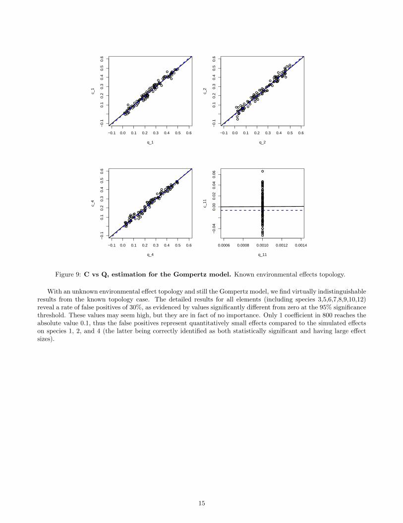
For the Gompertz model, this recovery is unbiased and extremely good (Fig. 9). Although the patterns ofenvironmental forcing are arguably simple here, there seem much better recovered - much less ambiguous - thanthe interactions between species.
14
●
●
●
●
●
●
●
●
●
●●
●
●
●
●
●
●
●
●
●
●
●
●
●
●
●
●
●
●
●
●
●
●
●
●
●
●
●
●
●
●
●●
●
●
●
●
●
●
●
●
●
●
●
●
●
●
●
●
●
●●
●●
●
●
●
●
●●
●
●
●
●
●
●
●●
●●
●
●
●
●
●
●
●
●
●
●●
●
●
●
●
●
●
●
●
●
−0.1 0.0 0.1 0.2 0.3 0.4 0.5 0.6
−0.
10.
10.
20.
30.
40.
50.
6
q_1
c_1
●
●
●●
●
●
●
●
●
●
●
●
●
●
●
●
●●
●
●
●
●
●
●
●
●
●
●
●
●
●
●
●
●●
●
●
●
●
●
●
●
●
●
●
●
●
●
●
●
●
●
●
●
●
●
●
●
●
●
●●
●
●
●
●
●
●
●
●
●
●
●
●
●
●
●
●●
●●
●
●
●
●
●
●
●
●
●
●
●
●
●●
●
●
●
●
●
−0.1 0.0 0.1 0.2 0.3 0.4 0.5 0.6
−0.
10.
10.
20.
30.
40.
50.
6
q_2
c_2
●
●
●
●
●
●
●
●
●
●
●
●
●
●
●
●
●
●
●
●
●
●
●
●
●
●
●
●
●
●●
●
●
●
●
●
●
●
●
●
●
●
●
●
●
●
●
●
● ●
●
● ●
●
●
●
●
●
●
●
●
●
●●
●
●
●
●
●
●
●
●●
●●
●
●●
●
●
●
●
●
● ●
●●
●
●
●
●
●
●
●
●
●
●
●
●
●
−0.1 0.0 0.1 0.2 0.3 0.4 0.5 0.6
−0.
10.
10.
20.
30.
40.
50.
6
q_4
c_4
●
●
●
●
●
●●
●
●
●
●
●
●
●
●
●●
●
●
●
●
●
●
●
●
●
●●
●
●●
●
●
●
●
●
●
●
●
●
●●
●
●
●
●
●
●
●
●
●●
●
●
●
●
●
●
●●
●
●
●
●
●
●
●
●
●
●
●
●
●
●●
●
●
●
●
●
●
●●
●
●
●
●
●
●
●
●
●
●
●
●
●
●
●
●
●
0.0006 0.0008 0.0010 0.0012 0.0014
−0.
040.
000.
020.
040.
06
q_11
c_11
Figure 9: C vs Q, estimation for the Gompertz model. Known environmental effects topology.
With an unknown environmental effect topology and still the Gompertz model, we find virtually indistinguishableresults from the known topology case. The detailed results for all elements (including species 3,5,6,7,8,9,10,12)reveal a rate of false positives of 30%, as evidenced by values significantly different from zero at the 95% significancethreshold. These values may seem high, but they are in fact of no importance. Only 1 coefficient in 800 reaches theabsolute value 0.1, thus the false positives represent quantitatively small effects compared to the simulated effectson species 1, 2, and 4 (the latter being correctly identified as both statistically significant and having large effectsizes).
15
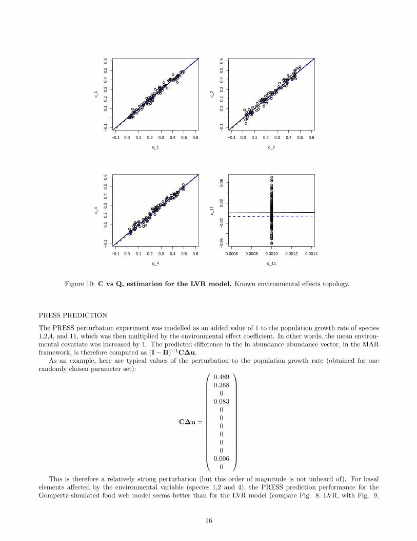
●
●
●
●
●
●
●
●
●
●●
●
●
●
●
●
●
●
●
●
●
●
●
●
●
●
●
●
●
●
●
●
●
●
●
●
●
●
●
●
●
●●
●
●
●
●
●
●
●
●
●
●
●●
●
●
●
●
●
●
●
●
●
●
●
●
●
●●
●
●
●
●
●
●
●
●
●●
●
●
●
●
●
●
●
●
●
●●
●
●
●
●
●
●
●
●
●
−0.1 0.0 0.1 0.2 0.3 0.4 0.5 0.6
−0.
10.
10.
20.
30.
40.
50.
6
q_1
c_1
●
●
●●
●
●
●
●
●
●
●
●
●
●
●
●
●
●
●
●
●
●
●
●
●
●
●
●
●
●
●
●
●
●●
●
●
●
●
●
●
●
●
●
●
●
●
●
●
●
●
●
●
●
●
●
●
●
●
●
●●
●
●
●
●
●
●
●
●
●
●
●
●
●
●
●
●●
●●
●
●
●
●
●
●
●
●
●
●
●
●
●●
●
●
●
●
●
−0.1 0.0 0.1 0.2 0.3 0.4 0.5 0.6
−0.
10.
10.
20.
30.
40.
50.
6
q_2
c_2
●
●
●
●
●
●
●
●
●
●
●
●
●
●
●
●
●
●
●
●
●
●
●
●
●
●
●
●
●
● ●
●
●
●
●
●
●
●
●
●
●
●
●
●
●
●
●
●
● ●
●● ●
●
●
●
●
●
●
●
●
●
●●
●
●
●
●
●
●
●
●●
●●
●
●
●●
●
●
●
●
● ●
●●
●
●
●
●
●
●
●
●
●
●
●
●
●
−0.1 0.0 0.1 0.2 0.3 0.4 0.5 0.6
−0.
10.
10.
20.
30.
40.
50.
6
q_4
c_4
●
●
●
●●
●●●
●
●
●●
●
●
●
●
●
●
●
●
●●
●
●
●
●
●●●
●
●
●
●
●●
●
●
●
●
●
●
●
●
●
●●
●
●
●
●
●
●
●
●
●
●
●
●
●●
●
●
●
●
●
●
●
●
●
●
●
●
●
●
●
●●
●
●
●
●
●●
●
●
●
●
●
●
●
●
●
●
●
●
●
●
●
●
●
0.0006 0.0008 0.0010 0.0012 0.0014
−0.
06−
0.02
0.02
0.06
q_11
c_11
Figure 10: C vs Q, estimation for the LVR model. Known environmental effects topology.
PRESS PREDICTION
The PRESS perturbation experiment was modelled as an added value of 1 to the population growth rate of species1,2,4, and 11, which was then multiplied by the environmental effect coefficient. In other words, the mean environ-mental covariate was increased by 1. The predicted difference in the ln-abundance abundance vector, in the MARframework, is therefore computed as (I−B)−1C∆u.
As an example, here are typical values of the perturbation to the population growth rate (obtained for onerandomly chosen parameter set):
C∆u =
0.4890.268
00.083
000000
0.0060
This is therefore a relatively strong perturbation (but this order of magnitude is not unheard of). For basal
elements affected by the environmental variable (species 1,2 and 4), the PRESS prediction performance for theGompertz simulated food web model seems better than for the LVR model (compare Fig. 8, LVR, with Fig. 9,
16

Gompertz). Thus for basal species PRESS prediction is only hard with LVR dynamics. On the other hand, elementsin the middle and top of the food web, that have weakly regulated dynamics, typically show outliers that impairthe PRESS predictions in all cases: Gompertz and LVR, known and unknown food web and environmental effecttopology5.
Clearly, as could be expected, the idea that MAR models can be used to predict the effects of PRESS pertur-bations may work only if those are extremely small (as a sort of sensitivity analysis, Gross & Edmunds, 2015), asany error in the identification of an effect tends to propagate through the B matrix. It may be possible to consideronly statistically significant elements in the B and C matrices, but as we have shown before, deciding which ofthese elements are non-zero based on the 95% CIs is somewhat prone to error. It would be better done using ap-propriate tools for perform model selection concurrently to estimation (e.g., the LASSO, Charbonnier et al., 2010;Michailidis & d’Alche Buc, 2013; Basu et al., 2015), which is a statistical endeavour unto itself and would requiremore evaluation (i.e., number of true positives, false positives, ROC curves, etc.).
5We do not show all the results because they are similar, PRESS predictions for LVR with unknown topology can be found herehttps://github.com/fbarraquand/MAR_foodWeb_MEE, version of record https://zenodo.org/record/1218024
17

●
●
●● ●●
●
●
●
●
●
●
●
●
●
●
●
●
●
●
●
●
●
●●
●
●●
●
●
●●
●●
●●
●
●
●
●
●
●
●
●
●
●
●
●
●
●
●●
●●
●
●
●
●
●
●
●●
●
●●
●●
●● ●
●
●
●
●
● ●
●
●
● ●
●
●
●
●
●
●
●
●
●
●
●
●
●
●
●
●
●
●
●
●
0.00 0.10 0.20
0.00
0.10
0.20
0.30
Species = 1
True Delta ln(N)
MA
R p
redi
cted
Del
ta ln
(N)
●
●
●●
●
●
●
●
●
●
●
●
●
●
●
●
●●
●
●
●
●
●
●
●
●
●
●
●
●
●
●
●
●
●
●
●
●
●●
●
●
●
●
●
●
●
●
●
●●
●
●
●
●
●
●●
●
●●●
●
●●
●
●
●
● ●
●
●
●
●
●
●
●
●
●
●
●
●
●
●●
●●
●●
●
●
●
●
●●
●
●
●
●
●
0.0 0.1 0.2 0.3 0.4
0.0
0.2
0.4
Species = 2
True Delta ln(N)
MA
R p
redi
cted
Del
ta ln
(N)
● ●●●●●●
●
●●●
●●●●
●
●
●●●
●
●●
●
●●●
●
●
●
●●
●●●●●
● ●
●
●●
●
●●●●
●●
●●●●
●●●●
●●●
●●
●
●●●●●●●
●●
●
●
●●●●
●
●●●
●●
●
●●
●
●●
●●
●
●●●●●●
●
−3.0 −2.0 −1.0 0.0
−2
01
23
4
Species = 3
True Delta ln(N)
MA
R p
redi
cted
Del
ta ln
(N)
●
●
●
●
●
●
●
●●
●●
●
●
●
●
●
●
●
●
●●
●
●
●
●
●
●
●
●
●
●
●
●
●●
●
●
●
●
●
●
●
●
●●
●
●
●
●
●
●
●●
●
●
●
●●
●
●
●
●
●
●
●
●
●●●
●
●
●●
●●
●
●
●
●
●
●
●
●
●
●
●
●
●●
●
●
●
●
●
●
●
●
●
●
●
0.1 0.2 0.3 0.4
0.0
0.2
0.4
Species = 4
True Delta ln(N)
MA
R p
redi
cted
Del
ta ln
(N)
●● ●● ●● ● ●
●● ●●●● ● ●●● ●●● ●●● ●● ● ●● ●●
●● ●
●●●
●
●● ●● ●● ●●●●● ●●● ●● ●● ●● ● ●● ● ●● ●●●●● ● ●●●●●
●● ●
●●● ●●● ●●●
●
● ●●●
●
●● ●● ● ●●
0.0 0.1 0.2 0.3 0.4
010
2030
Species = 5
True Delta ln(N)
MA
R p
redi
cted
Del
ta ln
(N)
●●
●
●
●
●
●●
●
●
●
●
●●
●
●
●
●
●
●
●
●●
●
●
●
● ●
●
●
●●●●●
●
●
●
●
●
●●
● ●
●
●
●
●
●
●
●
●
●
●
●
●
●●
●
●
●●
●
●
●●
● ●●
●●● ●●●
● ●●
●
●
●
●●●
●
● ●
●
●
●
●
● ●● ●●●
●
●●
0.00 0.10 0.20 0.30
−0.
50.
00.
5
Species = 6
True Delta ln(N)
MA
R p
redi
cted
Del
ta ln
(N)
●
●●
●●●
●
●●
● ●●
●
● ● ●● ●
●●●
●
●●
●●
●●
● ●●●
● ●
●
●●
●
●
●
●
●●
●
●
● ●
●● ●●●●●
●
●
●
●
●
●
●●
●
● ●● ●●●
●●
●●●●
●●
●●●●
●● ●
●
●●
●●●
●
●
●
● ●
●
●● ●
●
0.00 0.10 0.20 0.30
−1.
00.
01.
02.
0Species = 7
True Delta ln(N)
MA
R p
redi
cted
Del
ta ln
(N)
●
●
●●
●●
●
●
●●
●● ●
●●
●
●
● ●●
●●●
●
● ●●● ●
●
●
● ● ●●
●
●
●●
●
●
●●
●
●
● ● ●
●
●
●●
●
●● ●
●●
●
●● ●●
●
●
●
●●
●
●●●
●●
● ●
●●●●
●
●
● ●●
●●●
●●
●
●
● ●●● ●
●
●●
0.00 0.10 0.20
−1.
5−
0.5
0.5
Species = 8
True Delta ln(N)
MA
R p
redi
cted
Del
ta ln
(N)
●● ●●
●● ●
●
●●
●●●●● ●●● ●●
●
●●
●
●● ●
●
●●
●
●
●●
●
●●
●●
●●●●●● ●●
●
●●
●●●●●●
●●●●●● ●
●
●
●●●●
●
●●●●● ●● ●
●
●●●●●●● ●
●
●●●
●
●
●●●●●●
●
0.00 0.04 0.08
−4
−2
01
Species = 9
True Delta ln(N)
MA
R p
redi
cted
Del
ta ln
(N)
●● ●● ●● ● ● ●● ●●●●● ●●● ●●● ●●●●● ●●● ●● ●● ●●
●●
●
●● ●● ●●
●● ●●
● ●●● ●●
●
● ●● ●●●● ●●●●●●● ● ●●●●● ●● ●●●●●● ●● ●●
●
● ●●
● ●●● ●● ● ●●
0.0 0.2 0.4 0.6 0.8
020
6010
0
Species = 10
True Delta ln(N)
MA
R p
redi
cted
Del
ta ln
(N)
●● ●●
●
●●●
●●●●●
●●
●
●●● ●●● ●
●
●●●
●
●●●
●
●●●
●●
●
●●●● ● ●●
●
●●
●
●
●●
●
●●
●●●
●●●●
●●
● ●●●● ●
●●●●●●
●●
●●
●●●●
●
●●
●
● ●●●
●●●●●●●●
1 2 3 4 5
−80
−40
040
Species = 11
True Delta ln(N)
MA
R p
redi
cted
Del
ta ln
(N)
●●
●
● ●●
●
● ●●●●●
●● ●●● ●●●
●
●● ● ●●
●●●
●
●● ●●●
●
●
●● ●
●●
●●
●
●
●
●
●
●
●
●●
●
●●● ●
●● ●●
●
●●●● ● ●●●
●●●●
● ●
●
●● ●● ●
●
●
●●● ●
●
●
●●●
●
●●●
●
0.0 0.2 0.4
−4
02
46
8
Species = 12
True Delta ln(N)
MA
R p
redi
cted
Del
ta ln
(N)
Figure 11: PRESS true values vs predictions, LVR model, known topology. Black line: y = x.
18

●
●
●
●
●
●
●
●
●
●●●
●
●
●
●
●
●
●
●
●
●
●
●
●
●
●
●
●
●
●
●
●
●
●
●
●
●
●
●
●
●●
●
●
●
●
●
●
●
●
●
●
●
●
●
●
●
●
●
●
●
●●
●
●
●
●
●● ●
●
●
●●
●
●●
● ●
●
●
●
●
●
●
●
●
●
●●
●
●
●
●
●
●
●
●
●
0.00 0.10 0.20
0.00
0.10
0.20
Species = 1
True Delta ln(N)
MA
R p
redi
cted
Del
ta ln
(N)
●
●
●●
●
●
●
●
●●
●
●
●
●
●
●
●●
●
●
●
●
●
●
●
●
●
●
●
●
●
●
●
●●
●
●
●
●
●
●
●
●
●
●
●●
●
●
●
●
●
●
●
●
●
●
●
●
●●
●
●
●●
●
●
●
●●
●
●
●●
●
●
●
●●
●●
●
●
●●
●●
●
●
●
●
●
●
●●
●
●
●
●
●
0.0 0.2 0.4
0.0
0.2
0.4
Species = 2
True Delta ln(N)
MA
R p
redi
cted
Del
ta ln
(N)
● ●●●● ●●●●●●
●●●●● ●●●●●●●●
●●●● ●●● ●●
●
● ● ●● ●● ●●● ●●●●
●●●●●●
●●● ●●●●●●●●● ● ●●●
●
●
●● ●●● ●● ● ●
●●
●●● ●●●●
●
●●●
●●●●●● ●
−1.0 0.0 0.5
−10
−5
05
Species = 3
True Delta ln(N)
MA
R p
redi
cted
Del
ta ln
(N)
●
●
●
●
●
●
●
●
●
●●
●
●
●
●
●
●●
●
●
●
●
●
●
●
●
●
●
●
● ●
●
●
●
●
●
●
●
●
●
●
●
●
●
●
●
●
●
● ●
●● ●
●
●
●
●
●
●●
●
●
●
●
●
●
●
●
●
●
●
●●
●●
●
●
●●
●
●
●
●
● ●
●
●
●
●
●
●
●
●
●
●
●
●
●
●
●
0.1 0.3 0.5
0.0
0.2
0.4
Species = 4
True Delta ln(N)
MA
R p
redi
cted
Del
ta ln
(N)
●●●● ●● ●●●● ●● ●●
●●●●●
●● ● ●●● ●● ●● ● ●●●
●
● ●● ●●●●● ● ●●● ●● ● ●●●●● ●● ●●● ●
●
●
●● ● ●●●●●
●
●●●● ● ●●●●● ●
● ●●●●●● ●●● ●● ● ●● ●●●
0.0 0.2 0.4 0.6 0.8
−30
−20
−10
0
Species = 5
True Delta ln(N)
MA
R p
redi
cted
Del
ta ln
(N)
●● ●● ●
●
●
●●
●
●
●●
●
●
●●●
●
●●● ●
●
●●● ●
●●
●
●
●
●
●●●
●
●●
●●
●
●
●●
●
●
●●
●●●●● ● ●
●
● ●
● ●●
●
●●
●
●
●
●
●●
●●●
●
●
●
●
●● ●
●●
●
●●
●●
●
●●
●
●●
●
●
●●●
0.00 0.10 0.20 0.30
−1.
5−
0.5
0.5
Species = 6
True Delta ln(N)
MA
R p
redi
cted
Del
ta ln
(N)
●● ●
●
●
●●
●●
●
●
●
●
● ●
●
●●
●
●
●
●
●
●
●
●
● ●●
● ●
●●
●
●●
●
●
●● ●
●
●●●
●
●
●
●
●
●
●
●●
●
●
●
●●
●
●●
●●
●
●●
●
●
●●
●●●●
●
●
●●
●
●
●
●
●●
●●
●
●
●
●
●
●
●●
●
●
●
●●
0.00 0.10 0.20 0.30
0.0
0.5
1.0
Species = 7
True Delta ln(N)
MA
R p
redi
cted
Del
ta ln
(N)
●
●
●●
●
●
●
●
●
●●
●●
●
●●
● ●
●
●●
●●●
●
●
●
● ●
●
●
●
●
●
●
●●●
●
●●
●
●●
●
●
●
●●●
●
●
●
●●
●●●
●
●●
●
●
●
●
●●●
●● ●
●
●
●●●
●
●●
●
●●●
●
●
●
●●
●●
●
●
●●
●●
●●
●
●
0.0 0.1 0.2 0.3 0.4
−0.
40.
00.
40.
8
Species = 8
True Delta ln(N)
MA
R p
redi
cted
Del
ta ln
(N)
● ●●● ●● ●● ●●●● ●
●
●● ●●●● ●●● ●● ●● ●● ● ●●●
●
● ●●●●●●●●●● ●●● ● ●●● ●● ●● ●●●●●
●
●●
●
●●●●
●
●
●●●● ●● ●●●●●● ● ●●●●● ●●●●● ● ●● ● ●●
0.00 0.04
02
46
812
Species = 9
True Delta ln(N)
MA
R p
redi
cted
Del
ta ln
(N)
●●●●●● ●● ●●●●●●●●●●●●●● ●●●●● ●● ● ●●●●●●●●●●●● ●● ●● ●● ●●● ● ●● ●●●●●●●
●●● ●●●●
●
●
●
● ●●● ●●●●●● ●● ● ●●●●●●●● ●●● ●● ●●●
0.0 0.5 1.0 1.5
−20
0−
100
0
Species = 10
True Delta ln(N)
MA
R p
redi
cted
Del
ta ln
(N)
●●● ● ●●●●●●● ●● ●●
●●●●●●●●●●●
● ●●●●●●
●
●●● ●●●●●●●● ●●●
●
●● ●●●●
●●●●●
●
●
●●●●●●
●
●●
●●●●●●●●●●●●●●●●●●●●●●●●●● ●●●
0 5 10 20 30
−15
0−
5050
150
Species = 11
True Delta ln(N)
MA
R p
redi
cted
Del
ta ln
(N)
●
●
●● ●●
●
●
●
●
●
●●● ●
●
● ● ●● ● ●●●
●
●
●
●●
●●●
●
●
●●●
●●
●●● ●
●
●●
●
●●●
●●
●● ● ●
●
●●
●●
●●● ●●
●
●●
●●
●●
●●●
●●
●●●
●
● ●●
●
●●
●
●●
●
●
●●
●
●●●
●
0.05 0.15 0.25 0.35
−4
−2
02
Species = 12
True Delta ln(N)
MA
R p
redi
cted
Del
ta ln
(N)
Figure 12: PRESS true values vs predictions, Gompertz model, known topology. Black line: y = x.
19
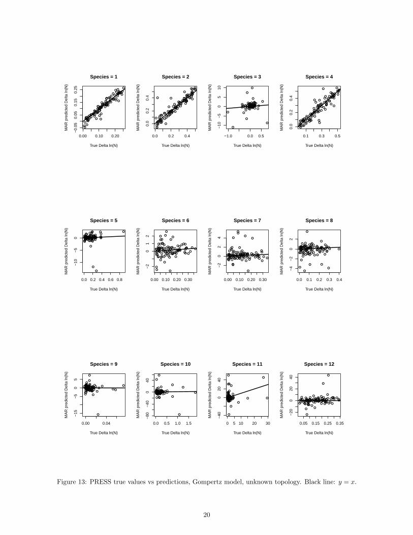
●●
●
●
●
●
●
● ●
●●
●
● ●
●
●
●
●
●
●
●
●
●●
●
●
●●
●
●
●
●
●
●
●
●
●
●
●
●
●
●●
●
●●
●
●
●
●
●●
●
●
●
●
●
●
●
●
●●
●●
●
●●
●
●●
●
●
●
●●
●
●
●
●●
●
●
●
●
●
●
●
●
●
●●
●
●
●●
●
●
●
●
●
0.00 0.10 0.20
−0.
050.
050.
150.
25Species = 1
True Delta ln(N)
MA
R p
redi
cted
Del
ta ln
(N)
●
●
●●
●
●
●
●
●●
●
●
●
●
●
●
●●
●
●
●
●
●
●
●
●
●
●
●
●
●
●
●
●●
●
●
●
●
●
●
●
●
●
●
●
● ●
●
●●
●
●
●
●
●
●
●
●
●●
●
●
●
●
●
●
●
●
●
●
●
●●
●
●
●
●●
●●
●
●
●
●
●
●
●
●
●
●
●
●●●
●
●
●
●
●
0.0 0.2 0.4
0.0
0.2
0.4
Species = 2
True Delta ln(N)
MA
R p
redi
cted
Del
ta ln
(N)
● ●●●● ●●●●●●●●●
●●
●●●●
●●●
●
●●●
●●●
●
●
●
●
● ● ●●
●●
●●● ●●●● ●
●
●●
●
●
●●
●●●●
●
●●●●● ●
●
●●
●●
●
● ●●● ●●
●● ●●
●
●● ●●●●
●
●●
●●
●●●
●
●
●
−1.0 0.0 0.5
−10
−5
05
10
Species = 3
True Delta ln(N)
MA
R p
redi
cted
Del
ta ln
(N)
●
●
●
●
●
●
●●
●●
●
●
●
●
●
●
●●
●
●
●
●
●
●
●
●
●
●
●
●
●
●
●
●
●
●
●
●
●●
●
●
●
●●
●
●
●
●
●
●
●
●
●
●
●
●
●
●
●
●
●
●
●
●●
●
●●
●
●
●
●
●●
●●
● ●
●
●
●
●
●●
●●
●
●
●
●
●
●
●
●
●
●
●
●
●
0.1 0.3 0.5
0.0
0.2
0.4
Species = 4
True Delta ln(N)
MA
R p
redi
cted
Del
ta ln
(N)
●●●●
●
●●●
●
● ●
●●
● ●●●●●
●● ● ●
●
●
●
● ●● ●
●
●●
●●
●●●
●●●● ● ●
●
●
●●
●
●●●●
●
●●●
●●●
●●
●● ● ●●●●
●
●
●
●●
●●
●●●●●
●● ●●●●
●
● ●●●
●
● ● ●● ●
●●
0.0 0.2 0.4 0.6 0.8
−10
−5
0
Species = 5
True Delta ln(N)
MA
R p
redi
cted
Del
ta ln
(N)
●●
●
● ●●●
●
●
●
●
●●
●
●
●
●
●●
●
●
●●●
●
●
●●
● ●
●
●
●
●
●
●
●
●
●●
●
●●
● ●
●
●●
●
●●
●
●
●
● ● ●●
●●
●●
●
●
●
●
●
●● ●
●
●
●●● ●
●
●
●
●
●
●●
●
●
●
●
●
● ●●
●
●
●
●
●●
●
●
●
0.00 0.10 0.20 0.30
−2
01
2
Species = 6
True Delta ln(N)
MA
R p
redi
cted
Del
ta ln
(N)
●● ●
●
●
●
● ●●●
●● ●● ● ●
● ●●●●
●
●
●
●
●
●
●●
●
●
●●
●
●●
●●
●●
●
● ●●●
●
●●
●
●● ●
●● ●
●
●
● ●●
●
●
● ●●
●
●
●●
●●
●
●●
● ●
●
●
●
●●●
●
●
●●●
●
●
●
●
●
●●●
●
●
●●
●
0.00 0.10 0.20 0.30
−2
02
4Species = 7
True Delta ln(N)
MA
R p
redi
cted
Del
ta ln
(N)
● ●● ●
●
●
●
●
●
● ●● ●
●
●●
●
●●
●
●
●
●
●●●
●
●●
●
●
●
●
●
●
●●●
●
●●
●●
●●
●
●●
●
●●●
●
● ● ●●●
●
●
●
●●
●
●
●
● ●
● ●
●
●
●
●●
●
●
●●
●
●
●●
●
●
●
●
●
●● ●
●
●
●●● ● ●
●
●
0.0 0.1 0.2 0.3 0.4
−4
−2
02
Species = 8
True Delta ln(N)
MA
R p
redi
cted
Del
ta ln
(N)
●●
●●
●● ●● ●●●● ●
●
●● ●●●●
●●●●●
●
● ●
●
●
●
●●
●●
●
●●●
●
●
●●●
●
●●
●
●
●●● ●● ●
●
●●●●
●
●●●
●
●
●● ●●
●
●●
●● ●●
●
●●●●● ●
●●●
●●
●
●●
●
●●
●●●
●
●
0.00 0.04
−15
−5
05
Species = 9
True Delta ln(N)
MA
R p
redi
cted
Del
ta ln
(N)
●●
●●●● ●● ●●
●●●
●●●●●●●●● ●●
●●● ●●
●
●
●●
●
●●●●●●●● ●●
●
●
●●
●
●●
● ●
●●●●●●●●● ●
● ●●
●
●
●●
●
●
●●● ●●●●●
● ●●● ●
●●
●●●●●
●
●● ●●●
●●
0.0 0.5 1.0 1.5
−80
−40
040
Species = 10
True Delta ln(N)
MA
R p
redi
cted
Del
ta ln
(N)
●
●
●● ●
●
●●●
●●
●●
●●
●●●●●●●●●
●
●
●●●●
●
●●
●
●●● ●
●●
●●●●●
●
●●
●
●
●
●●●
●
●
●●●
●
●
●●●●●
●●
●●
●
●
●●●●●●●
●
●●●
●
●●
●●●
●●●
●
●●●●
●●●
0 5 10 20 30
−40
020
40
Species = 11
True Delta ln(N)
MA
R p
redi
cted
Del
ta ln
(N)
●●
●●
●●
●●●
●●●
●● ●
●●
●●
● ● ●●●●
●● ●●
●
●●
●
●
●●●
● ●●●● ●
●
●
●
●●
●
●●●
●● ●
●
●
● ●●
●
●
●
● ●●●
●●
●
●
●
● ●●●
●
● ●● ●●
●●●
●
●●
●
●
●
●
●
●●● ● ●
●
●
0.05 0.15 0.25 0.35
−20
020
40
Species = 12
True Delta ln(N)
MA
R p
redi
cted
Del
ta ln
(N)
Figure 13: PRESS true values vs predictions, Gompertz model, unknown topology. Black line: y = x.
20
References
Aufderheide, H., Rudolf, L., Gross, T. & Lafferty, K.D. (2013) How to predict community responses to perturbationsin the face of imperfect knowledge and network complexity. Proceedings of the Royal Society B: Biological Sciences,280, 20132355.
Basu, S., Michailidis, G. et al. (2015) Regularized estimation in sparse high-dimensional time series models. TheAnnals of Statistics, 43, 1535–1567.
Charbonnier, C., Chiquet, J. & Ambroise, C. (2010) Weighted-lasso for structured network inference from timecourse data. Statistical applications in genetics and molecular biology, 9, 1–29.
Erbach, A., Lutscher, F. & Seo, G. (2013) Bistability and limit cycles in generalist predator–prey dynamics. Eco-logical Complexity, 14, 48–55.
Gross, K. & Edmunds, P.J. (2015) Stability of Caribbean coral communities quantified by long-term monitoringand autoregression models. Ecology, 96, 1812–1822.
Holmes, E.E., Ward, E.J. & Scheuerell, M.D. (2014) Analysis of multivariate time-series using the MARSS package.Technical report.
Michailidis, G. & d’Alche Buc, F. (2013) Autoregressive models for gene regulatory network inference: Sparsity,stability and causality issues. Mathematical biosciences, 246, 326–334.
Mutshinda, C.M., O’Hara, R.B. & Woiwod, I.P. (2011) A multispecies perspective on ecological impacts of climaticforcing. Journal of Animal Ecology, 80, 101–107.
Ovaskainen, O., Tikhonov, G., Dunson, D., Grøtan, V., Engen, S., Sæther, B. & Abrego, N. (2017) How are speciesinteractions structured in species-rich communities? a new method for analysing time-series data. ProceedingsBiological sciences, 284.
21
![On the Periodic Lotka-Volterra Competition Model › download › pdf › 82568635.pdf · PERIODIC LOTKA]VOLTERRA COMPETITION MODEL 59 the averages of the ‘‘birth rates’’](https://static.fdocuments.us/doc/165x107/5f1088e27e708231d44995e1/on-the-periodic-lotka-volterra-competition-model-a-download-a-pdf-a-periodic.jpg)


![Competitive Lotka-Volterra Population Dynamics with · PDF filearXiv:1102.2163v1 [math.PR] 10 Feb 2011 Competitive Lotka-Volterra Population Dynamics with Jumps Jianhai Bao1,3, Xuerong](https://static.fdocuments.us/doc/165x107/5aa5c9347f8b9a185d8dc6a8/competitive-lotka-volterra-population-dynamics-with-11022163v1-mathpr-10.jpg)