Bifurcations in Delayed Lotka-Volterra Intraguild...

MATIMYAS MATEMATIKA Journal of the Mathematical Society of the PhilippinesISSN 0115-6926 Vol. 37 Nos. 1-2 (2014) pp. 11-22

Bifurcations in Delayed Lotka-Volterra IntraguildPredation Model

Juancho A. ColleraDepartment of Mathematics and Computer Science

University of the Philippines Baguio

Baguio City, Philippines

[email protected]

Abstract

Omnivory is defined as feeding on more than one trophic level. An example of this isthe so-called intraguild predation (IG) which includes a predator and its prey that sharea common resource. IG predation models are known to exhibit interesting dynamicsincluding chaos. This work considers a three-species food web model with omnivory,where the interactions between the basal resource, the IG prey, and the IG predatorare of Lotka-Volterra type. In the absence of predation, the basal resource follows adelayed logistic equation or popularly known as Hutchinson’s equation. Conditionsfor the existence, stability, and bifurcations of all non-negative equilibrium solutionsare given using the delay time as parameter. Results are illustrated using numericalbifurcation analysis.

1 Introduction

Omnivory, as defined in [15], occurs when a population feeds on resources at more than onetrophic level. For example, a species feeding on its prey’s resource is called omnivorous.This particular type of tri-trophic community module is called intraguild (IG) predation[16], and was shown to be quite common in nature [1]. This three-species IG predationmodel includes top and intermediate predators termed as IG predator and IG prey, respec-tively, and a basal resource. The IG predator depends completely both on the IG prey andthe basal resource for its sustenance, while the IG prey depends solely on the basal resource.A study of a model of IG predation with non-linear functional responses in [13] showed thatomnivory stabilizes and enhances persistence of the three-species food web. However, amodel of Lotka-Volterra type with linear functional responses considered in [9] showed thatIG predation could have a destabilizing effect, and a criterion for co-existence of all threespecies is that the IG prey must be superior than the IG predator in competing for theshared basal resource. Lotka-Volterra IG predation models are known to exhibit interestingdynamics such as limit cycles [8], bistabity [10], and chaos [14, 19].

In this paper, we consider a Lotka-Volterra IG predation model where, in the absence ofthe IG predator and the IG prey, the basal resource grows according to the delayed logisticequation or more commonly known as the Hutchinson’s equation [3]. It should be notedthat there are several other ways of formulating the delayed logistic equation such as in[2], and in this paper, we use the so-called classical delayed logistic equation. Our delayedmodel generalizes the Lotka-Volterra IG predation models of [9] and [19] which are basically

11

12 Juancho A. Collera

systems of ODEs.

This paper is organized as follows. In Section 2, we introduce the delayed Lotka-VolterraIG predation model and discuss the existence of its equilibrium solutions. In Section 3, wegive the main results of this paper. These are the conditions for stability and bifurcationsof all non-negative equilibria using the delay time as parameter. In Section 4, we usenumerical continuation and bifurcation analysis to illustrate our results on the effects of thedelay time to our Lotka-Volterra IG predation model. We then end by giving a summaryand the thoughts of this paper.

2 The Model

We consider the following delayed Lotka-Volterra IG predation model

x(t) = [a0 − a1x(t− τ)− a2y(t)− a3z(t)]x(t),

y(t) = [−b0 + b1x(t)− b3z(t)] y(t), (1)

z(t) = [−c0 + c1x(t) + c2y(t)] z(t),

where x(t), y(t), and z(t) are the densities at time t of the basal resource, IG prey, andIG predator, respectively. In the absence of the IG predator and the IG prey, the basalresource grows according to the delay logistic equation [3, 18]. When τ = 0, we recover theODEs model in [19]. We refer to [19] for the description of the rest of the parameters in(1). Moreover, we use an initial condition (x(t), y(t), z(t)) = (x0, y0, z0) for t ∈ [−τ, 0] andwhere x0, y0, z0 ≥ 0.

An important characteristic of the IG predation is that it is a mixture of communitymodules such as competition and predation [8, 9, 16]. When a3 = c1 = 0, we obtain afood chain while if b3 = c2 = 0, we obtain exploitative competition (or shared resources)where two predators, in our case the IG predator and the IG prey, share a common resourceand the IG predator does not feed on the IG prey. Meanwhile, if a2 = b1 = 0, we obtainapparent competition (or shared predation), which in our model, the IG predator feeds onboth the IG prey and the basal resource but there is no predation on the basal resource bythe IG prey. In this case, the IG prey will go extinct.

2.1 Equilibrium Solutions

System (1) has five possible non-negative equilibrium solutions: E0 = (0, 0, 0), E1 = (K, 0, 0)where K = a0/a1, E2 = (A,B, 0) where A = b0/b1 and B = (a0b1 − a1b0)/a2b1, E3 =(C, 0, D) where C = c0/c1 and D = (a0c1−a1c0)/a3c1, and the positive equilibrium solutionE4 = (P/S,Q/S,R/S) where

P = a0b3c2 − a2b3c0 + a3b0c2,

Q = −a0b3c1 + a1b3c0 − a3b0c1 + a3b1c0,

R = a0b1c2 − a1b0c2 + a2b0c1 − a2b1c0,S = a1b3c2 − a2b3c1 + a3b1c2.

Since all parameters of system (1) are positive, we have K > 0, A > 0, and C > 0. Thus,E0 and E1 always exist. For E2 and E3 to exist, we require B > 0 and D > 0, respectively,or equivalently A < K and C < K, respectively. Now, if S is positive (resp. negative),

Bifurcations in Delayed Lotka-Volterra... 13

then each of P , Q, and R must also be positive (resp. negative) for E4 to be a positiveequilibrium. The following theorem summarizes these results.

Theorem 1. For system (1), the equilibrium solutions E0 = (0, 0, 0) and E1 = (K, 0, 0)always exist, while E2 and E3 exist provided a0b1 > a1b0 and a0c1 > a1c0, respectively, orequivalently, A < K and C < K, respectively. The positive equilibrium solution E4 exists ifP/S, Q/S, and R/S are all positive.

2.2 Local Stability of Equilibria

Let X(t) = [x(t), y(t), z(t)]T . Then, the linear system corresponding to (1) around anequilibrium solution E∗ = (x∗, y∗, z∗) is X(t) = M0X(t) +M1X(t− τ) where

M0 =

a0 − a1x∗ − a2y∗ − a3z∗ −a2x∗ −a3x∗b1y∗ −b0 + b1x∗ − b3z∗ −b3y∗c1z∗ c2z∗ −c0 + c1x∗ + c2y∗

and

M1 =

−a1x∗ 0 00 0 00 0 0

,and with corresponding characteristic equation

det(λI −M0 −M1e−λτ ) = 0. (2)

If all roots of (2) have negative real part, then the equilibrium solution E∗ is locally asymp-totically stable [18]. We can think of the roots of (2) as continuous functions of the delaytime τ , that is, λ = λ(τ). When τ = 0, (2) is a polynomial equation. In this case, thewell-known Routh-Hurwitz criterion can then be utilized to provide stability conditions forE∗. Now, consider the case when τ > 0. The following lemma is adopted from Corollary2.4 of [17] specifically for the characteristic equation (2).

Lemma 2. As τ is increased from zero, the sum of the orders of the roots of (2) in theopen right half-plane can change only if a zero appears on or crosses the imaginary axis.

This means that stability switch occurs at a critical value τ = τ0 where λ(τ0) is eitherzero or purely imaginary. The transversality condition d(Re λ)/dτ |τ=τ0 > 0 implies that theeigenvalues cross from left to right. Hence, if E∗ is stable at τ = 0, then, as τ is increased,it loses its stabilty at τ = τ0. Thus, E∗ is locally asymptotically stable when τ ∈ (0, τ0). Ifthere are no roots of (2) that cross the imaginary axis, then there are no stability switchesand in this case, we have absolute stability [4]. That is, E∗ remains stable for all delay timeτ > 0.

In the section that follows, we show that stability switch occurs at a Hopf bifurcationpoint. That is, a stable equilibrium solution E∗ loses its stability at τ = τ0 where λ(τ0)is purely imaginary while a small-amplitude limit cycle branching from this equilibriumsolution emerges. More precisely, we now state the Hopf Bifurcation Theorem [3, 18].Consider the one-parameter family of delay differential equations

x(t) = F (xt, ρ), (3)

where F : C×R→ Rn is twice continuously differentiable in its arguments, C = C ([−r, 0] ,Rn)is the space of continuous functions from [−r, 0] into Rn with r ≥ 0, xt(θ) = x(t + θ) for


xt ∈ C, and F (0, ρ) = 0 for all ρ. That is, φ = 0 is an equilibrium solution of (3) for allρ. Linearizing (3) about φ = 0, we obtain the linear system x(t) = L(ρ)xt. We assumethat the characteristic equation h(ρ, λ) = 0 corresponding to this linear system satisfies thefollowing:

(H1) h(0, λ) = 0 has a pair of simple imaginary roots ±iω0 with ω0 6= 0 and no other rootthat is an integer multiple of ω0.

Property (H1) implies that hλ(0, iω0) 6= 0. The implicit function theorem then guarantees,for small ρ, the existence of continuously differentiable family of roots λ(ρ) = α(ρ) + iω(ρ)satisfying λ(0) = iω0. We also assume that

(H2) the roots λ(ρ) cross the imaginary axis transversally as ρ increases from zero. Thatis, α′(0) > 0.

Theorem 3 (Hopf Bifurcation Theorem). Let (H1) and (H2) hold. Then, there exists ε0 >0, real-valued even functions ρ(ε) and T (ε) satisfying ρ(0) = 0 and T (0) = 2π/ω0 and a non-constant T (ε)-periodic function p(t, ε), with all functions being continuously differentiablein ε for |ε| < ε0, such that p(t, ε) is a solution of (3) and p(t, ε) = εq(t, ε) where q(t, 0) is a2π/ω0-periodic solution of q′ = L(0)q.

3 Main Results

In the following, we give conditions for the stability of each equilibrium solution of system(1) when τ > 0 using the technique mentioned above. When τ = 0, the stability analysis ofeach of the equilibrium solution of system (1) can be found in [14, Appendix A] and in [9]but in slightly different form. We mention them here for completeness.

At E0, the characteristic equation (2) becomes (λ− a0)(λ+ b0)(λ+ c0) = 0 whose rootsare a0 > 0, −b0 < 0 and −c0 < 0. Thus, we have the following result.

Theorem 4. The equilibrium solution E0 = (0, 0, 0) of system (1) is a local saddle pointand is unstable for all delay time τ > 0.

At E1, the characteristic equation (2) becomes

(λ− b1a2B/a1) (λ− c1a3D/a1)(λ+ a0e

−λτ) = 0. (4)

When τ = 0, (4) has roots −a0 < 0, b1a2B/a1, and c1a3D/a1. In this case, we see that E1

is locally asymptotically stable provided both B and D are negative, or equivalently A > Kand C > K. Recall from Theorem 1 that these conditions imply that both E2 and E3 donot exist. Suppose now that τ > 0, and A > K and C > K. It is known that all rootsof λ + a0e

−λτ = 0 have negative real part if and only if a0τ < π/2 (see for example [12,pp.70]). Thus, E1 is locally asymptotically stable if and only if τ < π/2a0.

Theorem 5. Suppose that (1) satisfies a1b0 > a0b1 and a1c0 > a0c1, or equivalently A > Kand C > K, respectively. Then, the equilibrium solution E1 = (K, 0, 0) is locally asymptoti-cally stable if and only if τ ∈ (0, τc) where τc = π/2a0. If τ = τc, then (1) undergoes a Hopfbifurcation at E1.

Example 1. The set of parameter values

(a0, a1, a2, a3, b0, b1, b3, c0, c1, c2) = (1, 0.5, 1, 0.6, 0.75, 0.25, 0.5, 0.5, 0.15, 0.3)


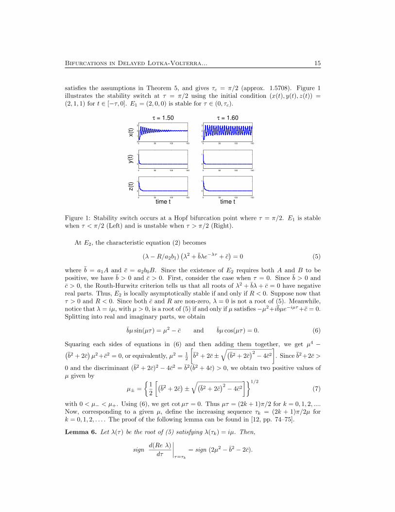
satisfies the assumptions in Theorem 5, and gives τc = π/2 (approx. 1.5708). Figure 1illustrates the stability switch at τ = π/2 using the initial condition (x(t), y(t), z(t)) =(2, 1, 1) for t ∈ [−τ, 0]. E1 = (2, 0, 0) is stable for τ ∈ (0, τc).

0 50 100 1500

1

2

3

x(t

)

τ = 1.50

0 50 100 150

0

1

y(t

)

0 50 100 150

0

1

time t

z(t

)

0 50 100 1500

1

2

3

τ = 1.60

0 50 100 150

0

1

0 50 100 150

0

1

time t

Figure 1: Stability switch occurs at a Hopf bifurcation point where τ = π/2. E1 is stablewhen τ < π/2 (Left) and is unstable when τ > π/2 (Right).


(λ−R/a2b1)(λ2 + bλe−λτ + c

)= 0 (5)

where b = a1A and c = a2b0B. Since the existence of E2 requires both A and B to bepositive, we have b > 0 and c > 0. First, consider the case when τ = 0. Since b > 0 andc > 0, the Routh-Hurwitz criterion tells us that all roots of λ2 + bλ + c = 0 have negativereal parts. Thus, E2 is locally asymptotically stable if and only if R < 0. Suppose now thatτ > 0 and R < 0. Since both c and R are non-zero, λ = 0 is not a root of (5). Meanwhile,notice that λ = iµ, with µ > 0, is a root of (5) if and only if µ satisfies −µ2+ibµe−iµτ+c = 0.Splitting into real and imaginary parts, we obtain

bµ sin(µτ) = µ2 − c and bµ cos(µτ) = 0. (6)

Squaring each sides of equations in (6) and then adding them together, we get µ4 −(b2 + 2c

)µ2+ c2 = 0, or equivalently, µ2 = 1

2

[b2 + 2c±

√(b2 + 2c

)2 − 4c2]. Since b2+2c >

0 and the discriminant (b2 + 2c)2 − 4c2 = b2(b2 + 4c) > 0, we obtain two positive values ofµ given by

µ± =

{1

2

[(b2 + 2c

)±√(

b2 + 2c)2 − 4c2

]}1/2

(7)

with 0 < µ− < µ+. Using (6), we get cotµτ = 0. Thus µτ = (2k + 1)π/2 for k = 0, 1, 2, ....Now, corresponding to a given µ, define the increasing sequence τk = (2k + 1)π/2µ fork = 0, 1, 2, . . . . The proof of the following lemma can be found in [12, pp. 74–75].

Lemma 6. Let λ(τ) be the root of (5) satisfying λ(τk) = iµ. Then,

signd(Re λ)

dτ

∣∣∣∣τ=τk

= sign (2µ2 − b2 − 2c).


For µ = µ±, define the sequence τ±k = (2k+ 1)π/2µ± for k = 0, 1, 2, . . . correspondingly,and let τ±0 = τµ± . Since 0 < µ− < µ+, we have τµ+

< τµ− , and hence τµ+is the smallest

amongst all τ±k . From (7), we have 2µ2+ − b2 − 2c > 0. Thus, at τ = τµ+ (or equivalently at

µ = µ+), the quantity d(Re λ)dτ is positive by Lemma 6. This, together with Theorem 3, we

have the following result.

Theorem 7. Suppose that in system (1), a0b1c2 + a2b0c1 < a1b0c2 + a2b1c0 or equivalentlyR < 0. Then, the equilibrium solution E2 = (A,B, 0) of (1) is locally asymptotically stablewhenever τ ∈ (0, τµ+

). If τ = τµ+, then system (1) undergoes a Hopf bifurcation at E2.

Example 2. Using the same set of parameters and initial condition as in Example 1 withb1 changed to 0.50, the assumptions in Theorem 7 are satisfied. Figure 2 illustrates thestability switch at τ = τµ+

= 1.6573 approximately.

0 50 100 1500

1

2

3

x(t

)

τ = 1.50

0 50 100 150

0

1

y(t

)

0 50 100 150

0

1

time t

z(t

)

0 50 100 1500

1

2

3

τ = 1.75

0 50 100 150

0

1

0 50 100 150

0

1

time t

Figure 2: Stability switch occurs at a Hopf bifurcation where τ = τµ+ = 1.6573 approxi-mately. The equlibrium solution E2 = (1.50, 0.25, 0.00) is stable when τ < τµ+

(Left) andis unstable when τ > τµ+

(Right).

A similar condition for the stability of E3 can be obtained using the same analysis usedfor E2, and is given in the following theorem.

Theorem 8. Suppose that in system (1), a1b3c0 + a3b1c0 < a0b3c1 + a3b0c1 or equivalentlyQ < 0. Let b = a1C, c = a3c0D, and

ν+ =

{1

2

[(b2 + 2c

)+

√(b2 + 2c

)2− 4c2

]}1/2

.

Then, the equilibrium solution E3 = (C, 0, D) of (1) is locally asymptotically stable wheneverτ ∈ (0, τν+) where τν+ = π/2ν+. If τ = τν+ , then system (1) undergoes a Hopf bifurcationat E3.


λ3 + aλ+ b+ (cλ2 + d)e−λτ = 0 (8)

where a = (PQa2b1 + PRa3c1 + QRb3c2)/S2, b = PQR(a3b1c2 − a2b3c1)/S3, c = a1P/S,and d = PQRa1b3c2/S

3. Note here that b + d = PQR/S2. Order-three quasi-polynomialswith single delay, different to (8), have been studied in [5, 11]. We follow a similar method


used in [5] to analyze the distribution of the roots of (8) on the complex plane. When τ = 0,then (8) reduces to

λ3 + cλ2 + aλ+ (b+ d) = 0. (9)

The Routh-Hurwitz criterion tells us that all roots of (9) have negative real part if and onlyif the following inequalities hold: a, c, b + d > 0 and ac− (b + d) > 0. If S < 0, then P , Q,and R must all be negative for E4 to be a positive equilibrium. This implies that a > 0,c > 0, and b+ d < 0, and thus, E4 is unstable. If S > 0, then each of P , Q, and R must bepositive for E4 to be a positive equilibrium. In this case, a, c, and b+d are all positive. Now,notice that if in addition to the assumption that S > 0, we also have b < 0 (or equivalentlya2b3c1 > a3b1c2), then ac− (b+ d) = a1P

2(Qa2b1 +Ra3c1)/S3 − b > 0. Hence, for the casewhen τ = 0, E4 is locally asymptotically stable whenever S > 0 and b < 0.

Suppose now that τ > 0, and assume that S > 0 and b < 0. If λ = 0 is a root of (8),then b + d = 0. However, b + d 6= 0 since b + d = PQR/S2 and none of P , Q, and R isequal to zero. Thus, λ = 0 is not a root of (8). If λ = iω, with ω > 0, is a root (8), then−iω3 + iaω + b+ (−cω2 + d)e−iωτ = 0. Splitting into real and imaginary parts, we get

(cω2 − d) cosωτ = b, and (cω2 − d) sinωτ = ω3 − aω. (10)

Squaring each sides of these equations and then adding corresponding sides give

ω6 + αω4 + βω2 + γ = 0 (11)

where α = −2a− c2, β = a2 + 2cd, and γ = b2−d2. We claim that α < 0, β > 0, and γ < 0.To see this, observe that since S > 0, we have P,Q,R > 0 and consequently, a, c, and d areall positive. Immediately, we see that α < 0 and β > 0. Meanwhile, the assumptions S > 0and b < 0 gives b + d > 0 and b − d < 0, respectively. As a result, γ = (b + d)(b − d) < 0.We now show that (11) has at least one positive root. Let h(u) = u3 + αu2 + βu + γ,and note that if the equation h(u) = 0 has a positive root u = u0, then (11) has a posi-tive root ω0 =

√u0. Now, notice that h′(u) = 3u2 + 2αu + β = 0 has two positive roots

u± = (−α ±√α2 − 3β )/3 with 0 < u− < u+. Since h(0) = γ < 0, h′(0) = β > 0,

and h′′(0) = 2α < 0, we know that the graph of h passes through the point (0, γ) belowthe horizontal axis, and then increases in a concave down manner. The continuity of hand the fact that h increases without bound as u → +∞ guarantee that h has at leastone positive root u0. That is, (11) has a positive root ω0 =

√u0, and therefore (8) has

purely imaginary roots λ = ±iω0. Noting that a local maximum of h occurs at u = u− anda local minimum of h occurs at u = u+, we see that the graph of the cubic polynomial his increasing on (0, u−) and on (u+,+∞). Moreover, we either have 0 < u0 < u− or u0 > u+.

If the equation h(u) = 0 has more than one positive roots, then it must have exactlythree positive roots so that ω is a simple root of (11). Using the first equation in (10), for

a given ω, define its corresponding increasing sequence τk = 1ω

[cos−1

(b

cω2−d

)+ 2πk

]for

k = 0, 1, 2, .... Specifically, for a given ω, we get a corresponding τ0. Among the three positiveroots of the equation h(u) = 0, we then choose u0 so that ω = ω0 =

√u0 has corresponding

τ0 that is smallest. This guarantees that a pair of purely imaginary eigenvalues first occursat τ = τ0.

Lemma 9. Let λ(τ) be the root of (8) satisfying λ(τk) = iω0. Then,

d(Re λ)

dτ

∣∣∣∣τ=τk

> 0.


Proof. From (8),[(3λ2 + a) + (2cλ− (cλ2 + d)τ)e−λτ

] dλdτ− λ(cλ2 + d)e−λτ = 0.

Consequently, (dλ

dτ

)−1=

2cλ+ (3λ2 + a)eλτ

λ(cλ2 + d)− τ

λ

=2c

cλ2 + d− 3λ2 + a

λ(λ3 + aλ+ b)− τ

λ

since eλτ/(cλ2 + d) = −1/(λ3 + aλ+ b) using (8). Hence,

sign

{d (Re λ)

dτ

}λ=iω0

= sign

{Re

(dλ

dτ

)−1}λ=iω0

= sign

{Re

2c

cλ2 + d+Re

−3λ2 − aλ4 + aλ2 + bλ

}λ=iω0

= sign

{Re

2c

−cω20 + d

+Re3ω2

0 − aω40 − aω2

0 + ibω0

}= sign

{−2c

cω20 − d

+(3ω2

0 − a)(ω40 − aω2

0)

(ω40 − aω2

0)2 + (bω0)2

}= sign

{−2c

cω20 − d

+(3ω2

0 − a)(ω20 − a)

(ω30 − aω0)2 + b2

}= sign

{−2c

cω20 − d

+(3ω2

0 − a)(ω20 − a)

(cω20 − d)2

}since (ω3

0 − aω0)2 + b2 = (cω20 − d)2 from (10). Thus,

sign

{d (Re λ)

dτ

}λ=iω0

= sign{−2c(cω2

0 − d) + (3ω20 − a)(ω2

0 − a)}

= sign{

3ω40 + (−4a− 2c2)ω2

0 + (a2 + 2cd)}

= sign{

3ω40 + 2αω2

0 + β}.

Since h is increasing on the intervals (0, u−) and (u+,∞), and u0 belongs to (0, u−) or to(u+,∞), we have h′(u0) = 3u20 + 2αu0 + β > 0. This implies that 3ω4

0 + 2αω20 + β > 0 since

ω0 =√u0. Thus,

sign

{d (Re λ)

dτ

}λ=iω0

= sign{

3ω40 + 2αω2

0 + β}

= +1

and this completes the proof.

By Lemma 9, d(Re λ)dτ

∣∣∣τ=τ0

> 0. This, together with Theorem 3 give the following result.

Theorem 10. Suppose that in system (1), a1b3c2 + a3b1c2 > a2b3c1 and a2b3c1 > a3b1c2(or equivalently S > 0 and b < 0, respectively). Then, the positive equilibrium solutionE4 of (1) is locally asymptotically stable whenever τ ∈ (0, τ0). If τ = τ0, then system (1)undergoes a Hopf bifurcation at E4.


Example 3. Using the same set of parameters as in Example 1 with b1 = 1 and c1 = 0.42,the assumptions in Theorem 10 are satisfied. Using the initial condition (x(t), y(t), z(t)) =(0.78, 0.58, 0.06) for t ∈ [−τ, 0], Figure 3 illustrates the stability switch at τ = τ0 = 1.7438approximately.

50 100 150 200 250 300 350 400 450

0.76

0.77

0.78

0.79

0.8

x(t

)

τ = 1.65

50 100 150 200 250 300 350 400 450

0.56

0.57

0.58

0.59

0.6

y(t

)

50 100 150 200 250 300 350 400 450

0.04

0.05

0.06

0.07

0.08

time t

z(t

)

0 50 100 150 200 250 300 350 400 4500

1

2

x(t

)

τ = 1.85

50 100 150 200 250 300 350 400 450

0

1

2

y(t

)

0 50 100 150 200 250 300 350 400 450

0

0.1

0.2

time t

z(t

)Figure 3: Stability switch occurs at τ = τ0 = 1.7438 (approx.). The positive equilibriumsolution E4 = (0.7778, 0.5778, 0.0556) is stable for τ < τ0 (Left) and is unstable when τ > τ0(Right).

4 Numerical Continuation

Recall that for τ = 0, E4 is locally asymptotically stable whenever S > 0 and b < 0. Abranch of equilibrium solutions can be obtained by following or continuing this equilibriumsolution in DDE-Biftool [6] using the delay time τ as parameter. DDE-Biftool is a numericalcontinuation and bifurcation analysis tool developed by Engelborghs et al [7]. We use thesame set of parameters and initial condition used in Example 3. In Figure 4, the top panelshows the branch of equilibrium solutions (horizontal line) obtained in DDE-Biftool, wheregreen and magenta represents the stable and unstable parts of the branch, respectively. Achange of stability occurs at a Hopf bifurcation point marked with (∗) where τ = τ0. Again,we use DDE-biftool to continue this Hopf point into a branch of periodic solutions. Weobtained a stable branch of periodic solutions and is shown as the green curve in the toppanel of Figure 4. Here, the vertical axis gives a measure of the maximum value of theoscillation of the periodic solutions in the x(t) component. The middle and bottom panelscorrespond to the same bifurcation diagram as the top panel but for the y(t) and the z(t)components.

Figure 4 illustrates the results of Theorem 10, that is, the stability switch at τ = τ0and the occurrence of Hopf bifurcation. Numerical continuations show that, as the positiveequilibrium E4 loses its stability, the branch of periodic solutions that emerges from theHopf point is stable. Biologically, this means that the three species still persist and the onlydifference now is that the three populations are oscillating.

5 Conclusion

We studied a delayed Lotka-Volterra IG predation model where, in the absence of predation,the basal resource grows according to the delayed logistic equation. By first considering thecase where τ = 0, stability conditions for the all non-negative equilibria are established usingthe well-known Routh-Hurwitz criterion. For τ > 0, we showed that stability switch occurs


1.74 1.75

0.8

1

x(t

)

1.74 1.75

0.6

0.7

y(t

)

1.74 1.75

0.056

0.06

0.064

Delay Time τ

z(t

)τ

0

τ0

τ0

Figure 4: Stable branch of periodic solutions emerges from the Hopf bifurcation point markedwith (∗) where τ = τ0.

at a Hopf bifurcation where the stable equilibrium becomes unstable. Moreover, numericalcontinuation shows that a stable branch of periodic solutions emerges from the Hopf pointas the positive equilibrium solution becomes unstable. This means that by increasing thedelay time the positive equilibrium could become unstable. However, since the periodicorbit that will emerge is stable, all three species will still persist.

Acknowledgement

The author acknowledges the support of the University of the Philippines Baguio and fund-ing from the Diamond Jubilee Professorial Chair Award.

References

[1] M. Arim, P.A. Marquet, Intraguild predation: a widespread interaction related tospecies biology, Ecol. Lett. 7(7) (2004) 557–564.

[2] J. Arino, W. Lin, G.S.K. Wolkowicz, An alternative formulation for a delayed logisticequation, J. Theor. Biol. 241(1) (2006) 109–119.

[3] O. Arino, M.L. Hbid, and E. Ait Dads (Eds.), Delay Differential Equations and Appli-cations, Springer, Berlin, 2006.

[4] F. Brauer, Absolute stability in delay equations, J. Differ. Equations 69(2) (1987)185–191.

[5] R.V. Culshaw, S. Ruan, A delay-differential equation model of HIV infection of CD4+

T-cells, Math. Biosci. 165(1) (2000) 27–39.


[6] K. Engelborghs, T. Luzyanina, D. Roose, Numerical bifurcation analysis of delay dif-ferential equations using DDE-BIFTOOL, ACM T. Math. Software 28(1) (2002) 1–21.

[7] K. Engelborghs, T. Luzyanina, G. Samaey, DDE-BIFTOOL v. 2.00: a Matlab packagefor bifurcation analysis of delay differential equations, Report TW-330, Department ofComputer Science, K.U. Leuven, Leuven, Belgium, 2001.

[8] R.D. Holt, Community modules, in: Multitrophic interactions in terrestrial ecosystems,36th Symposium of the British Ecological Society, Blackwell Science, Oxford, 1997, pp.333–349

[9] R.D. Holt, G.A. Polis, A theoretical framework for intraguild predation, Am. Nat.(1997) 745–764.

[10] S.B. Hsu, S. Ruan, T.H. Yang, Analysis of three species Lotka-Volterra food web modelswith omnivory, J. Math. Anal. Appl. (in press).

[11] P. Katri, S. Ruan, Dynamics of human T-cell lymphotropic virus I (HTLV-I) infectionof CD4+ T-cells, C. R. Biol. 327(11) (2004) 1009–1016.

[12] Y. Kuang, Delay Differential Equations with Applications in Population Dynamics,Academic Press, New York, 1993.

[13] K. McCann, A. Hastings, Reevaluating the omnivorystability relationship in food webs,P. Roy. Soc. Lond. B Bio. 264(1385) (1997) 1249–1254.

[14] T. Namba, K. Tanabe, N Maeda, Omnivory and stability of food webs, Ecol. Complex.5(2) (2008) 73–85.

[15] S.L. Pimm, J.H. Lawton, On feeding on more than one trophic level, Nature 275(5680)(1978) 542–544.

[16] G.A. Polis, C.A. Myers, R.D. Holt, The ecology and evolution of intraguild predation:potential competitors that eat each other, Annu. Rev. Ecol. Syst. (1989) 297–330.

[17] S. Ruan, J. Wei, On the zeros of transcendental functions with applications to stabilityof delay differential equations with two delays, Dynam. Cont. Dis. Ser. A 10 (2003)863–874.

[18] H. Smith, An Introduction to Delay Differential Equations with Applications to the LifeSciences, Springer, New York, 2011.

[19] K. Tanabe, T. Namba, Omnivory creates chaos in simple food web models, Ecology86(12) (2005) 3411–3414.

Bifurcations in Delayed Lotka-Volterra Intraguild...

Documents

Transcript of Bifurcations in Delayed Lotka-Volterra Intraguild...