Supporting hyperplanes

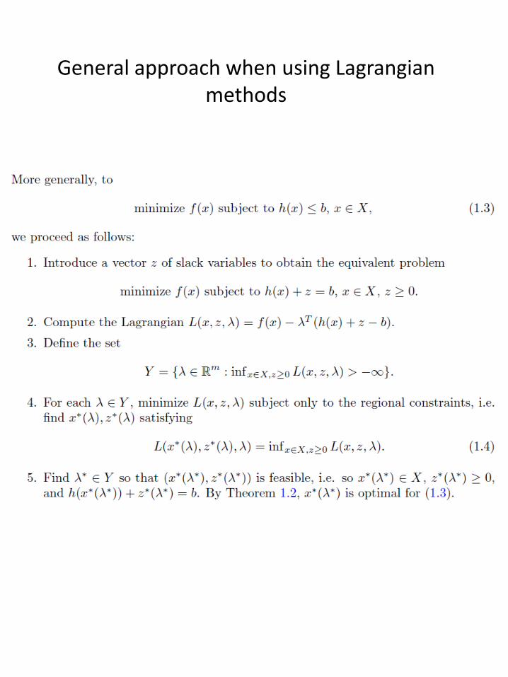
General approach when using Lagrangianmethods

Lecture 1 homework

Shadow prices

A linear programming problem

The simplex tableau

Simple example with cycling

The pivot rule being used is steepest descent: choose the column with the most negative entry in the bottom row.

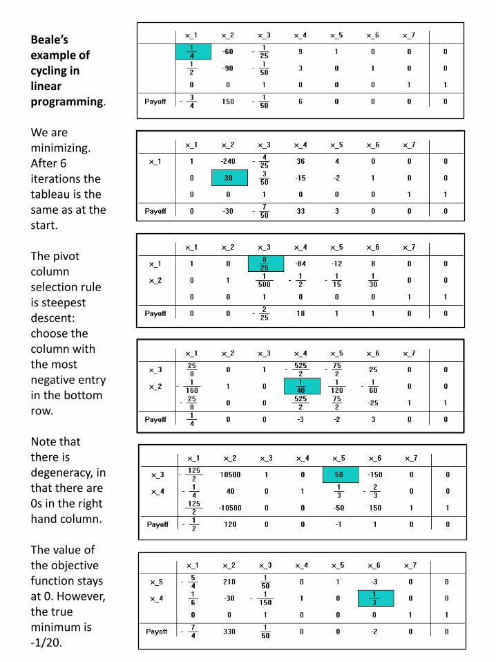
Beale’s example of cycling in linear programming.

We are minimizing. After 6 iterations the tableau is the same as at the start.

The pivot column selection rule is steepest descent: choose the column with the most negative entry in the bottom row.

Note that there is degeneracy, in that there are 0s in the right hand column.

The value of the objective function stays at 0. However, the true minimum is -1/20.

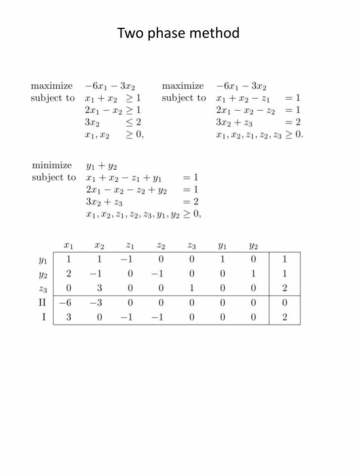
Two phase method

Dual simplex algorithm

Gomory’s cutting plane method

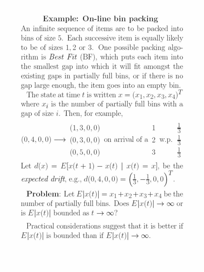
Many complex processes can be modelled by (countably) infinite, multidimensional Markov chains. Unfortunately, theoretical techniques for analysing infinite Markov chains are for the most part limited to three or fewer dimensions. In this paper we propose a computer-aided approach to the analysis of higher-dimensional domains, using several open problems about the average-case behavior of the Best Fit bin packing algorithm as case studies. We show how to use dynamic and lienar programming to construct potential functions that when applied to suitably modified multi-step versions of our original Markov chain, yield drifts that are bounded away from 0. This enables us to completely classify the expected behavior of Best Fit under discrete uniform distributions U{J, K) when K is small. In addition, we can answer yes to the long-standing open question of whether there exist distributions of this form for which Best Fit yields linearly-growing waste. The proof of the latter theorem relies on a 24-hour computation, and although its validity does not depend on the linear programming package we used, it does rely on the correctness of our dynamic programming code and of our computer’s implementation of the IEEE floating point standard.

The running time of algorithms

Relationship between complexity classes

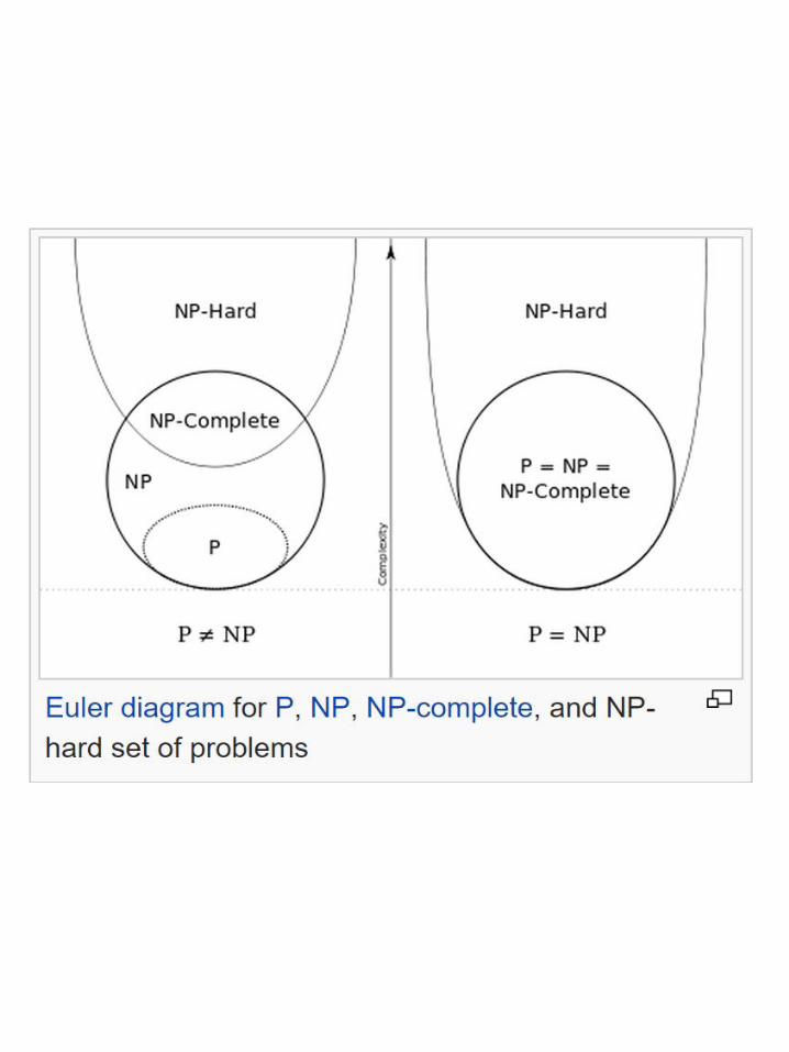
P v NP Suppose that you are organizing housing accommodations for a group of four hundred university students. Space is limited and only one hundred of the students will receive places in the dormitory. To complicate matters, the Dean has provided you with a list of pairs of incompatible students, and requested that no pair from this list appear in your final choice. This is an example of what computer scientists call an NP-problem, since it is easy to check if a given choice of one hundred students proposed by a coworker is satisfactory (i.e., no pair taken from your coworker's list also appears on the list from the Dean's office), however the task of generating such a list from scratch seems to be so hard as to be completely impractical. Indeed, the total number of ways of choosing one hundred students from the four hundred applicants is greater than the number of atoms in the known universe! Thus no future civilization could ever hope to build a supercomputer capable of solving the problem by brute force; that is, by checking every possible combination of 100 students. However, this apparent difficulty may only reflect the lack of ingenuity of your programmer. In fact, one of the outstanding problems in computer science is determining whether questions exist whose answer can be quickly checked, but which require an impossibly long time to solve by any direct procedure. Problems like the one listed above certainly seem to be of this kind, but so far no one has managed to prove that any of them really are so hard as they appear, i.e., that there really is no feasible way to generate an answer with the help of a computer. Stephen Cook and Leonid Levin formulated the P (i.e., easy to find) versus NP (i.e., easy to check) problem independently in 1971.

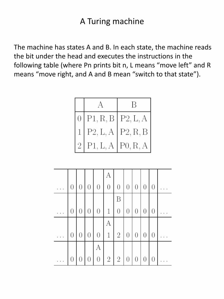
The machine has states A and B. In each state, the machine reads the bit under the head and executes the instructions in the following table (where Pn prints bit n, L means “move left” and R means “move right, and A and B mean “switch to that state”).

A Turing machine

• Satisfiability: the boolean satisfiability problem for formulas in conjunctive normal form (SAT)

• 0–1 integer programming (A variation in which only the restrictions must be satisfied, with no optimization)• Clique (independent set problem)

• Set packing• Vertex cover

• Set covering• Feedback node set• Feedback arc set• Directed Hamilton circuit

• Undirected Hamilton circuit• Satisfiability with at most 3 literals per clause (equivalent to 3-SAT)

• Chromatic number (also called the Graph Coloring Problem)

• Clique cover• Exact cover

• Hitting set• Steiner tree• 3-dimensional matching• Knapsack (Karp's definition of

Knapsack is closer to Subset sum)• Job sequencing• Partition

• Max cut

https://en.wikipedia.org/wiki/Karp’s_21_NP-complete_problems

Firing squad problem

The name of the problem comes from an analogy with real-world firing squads: the goal is to design a system of rules according to which an officer can so command an execution detail to fire that its members fire their rifles simultaneously.

More formally, the problem concerns cellular automata, arrays of finite state machines called "cells" arranged in a line, such that at each time step each machine transitions to a new state as a function of its previous state and the states of its two neighbors in the line. For the firing squad problem, the line consists of a finite number of cells, and the rule according to which each machine transitions to the next state should be the same for all of the cells interior to the line, but the transition functions of the two endpoints of the line are allowed to differ, as these two cells are each missing a neighbor on one of their two sides.

The states of each cell include three distinguished states: "active", "quiescent", and "firing", and the transition function must be such that a cell that is quiescent and whose neighbors are quiescent remains quiescent. Initially, at time t = 0, all states are quiescent except for the cell at the far left (the general), which is active. The goal is to design a set of states and a transition function such that, no matter how long the line of cells is, there exists a time t such that every cell transitions to the firing state at time t, and such that no cell belongs to the firing state prior to time t.

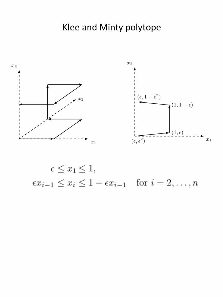
Klee and Minty polytope

The Hirsch conjecture

The ellipsoid method

Ellipsoid method

A basic feasible flow is a spanning tree

Network simplex algorithm