Supply, Demand, Institutions, and Firms: A Theory ofLabor Market Sorting and the Wage Distribution ∗

Daniel Haanwinckel†

Job Market Paper

December 31, 2018Click here for the latest version

Abstract

This paper builds a tractable framework for analyzing the equilibrium effects of labor sup-ply shocks, technical change, and minimum wages in an imperfectly competitive labor marketenvironment with worker and firm heterogeneity. Goods are produced using task-based tech-nologies exhibiting imperfect substitution between worker types. Firms specialize in the pro-duction of particular goods, which leads to differences in task requirements, entry costs, andworkplace amenities. These differences generate firm heterogeneity in skill intensity, size, andwages. The model has three advantages relative to the canonical supply-demand-institutionsframework typically used to study trends in wage inequality. First, task-based productionwith multiple worker types allows for plausibly rich formulations of the structure of technicalchange. Second, the model accounts for equilibrium effects of minimum wages, compressingthe wage distribution and generating spillovers on quantiles where the minimum wage does notbind. Third, the model makes predictions regarding labor market sorting and cross-firm wagedispersion. I take a simple version of the model to Brazilian matched employer-employee dataand show that it can fit several aspects of wage inequality: differences in mean log wages be-tween educational groups, within education group variances, and two-way variance decompo-sitions of log wages into worker and firm components. The model also matches reduced-formestimates of minimum wage spillovers. I use the estimated parameters to decompose observedchanges in inequality and sorting into components attributable to increasing schooling achieve-ment, technical change, and a rising minimum wage. Falling wage inequality in Brazil is pri-marily due to the minimum wage, while rising worker-firm assortativeness is found to be drivenby technical change. The decomposition exercise also illustrates how responses to supply anddemand shocks differ qualitatively from those predicted by models with a representative firm.

∗I would like to thank David Card, Fred Finan, Andrés Rodríguez-Clare, and especially Pat Kline for their guidanceand support. This paper benefited from comments from Ben Faber, Thibault Fally, Cecile Gaubert, Nicholas Li,Juliana Londoño-Vélez, Piyush Panigrahi, Raffaele Saggio, Yotam Shem-Tov, José P. Vásquez-Carvajal, Thaís Vilela,Christopher Walters, and other colleagues and faculty at UC Berkeley. I also thank Lorenzo Lagos and David Card forproviding code to clean the RAIS data set.†PhD candidate, Department of Economics, University of California, Berkeley. haanwinckel@berkeley.edu

1 Introduction

A central task in labor economics is understanding the source of changes in the wage distribution.Three sets of explanatory factors have received the most attention in this literature: trends in therelative supply of skills, such as increasing college completion rates; shocks to relative demandfor skills, such as skill-biased technical change; and changes in labor market institutions, such asminimum wages. The dominant approach in this literature employs competitive labor market mod-els with a constant elasticity of substitution production function to quantify the relative importanceof these factors (Bound and Johnson, 1992; Katz and Murphy, 1992; Card and Lemieux, 2001).This approach successfully captures trends in mean log wage gaps between broadly defined workergroups (e.g., college versus high school) and is still used by leading researchers (Autor, 2014). Butit has limitations on three fronts. First, it cannot match other measures of wage inequality using itsparsimonious formulation of demand shocks as skill-biased technical change (Card and DiNardo,2002; Autor, Katz and Kearney, 2008). Second, the focus on between-group wage gaps also pre-vents that approach from fully accounting for the effects of changing minimum wages (DiNardo,Fortin and Lemieux, 1996; Lee, 1999). Third, it cannot be used to study between-firm wage dis-persion for similar workers, a phenomenon that is now extensively documented (Manning, 2011;Hornstein, Krusell and Violante, 2011; Card et al., 2018) and that some economists suggest mighthave implications for the evolution of inequality (Card, Heining and Kline, 2013; Alvarez et al.,2018; Song et al., 2018).

Different strands of the wage inequality literature endeavor to address these limitations. Task-basedmodels of comparative advantage are used to evaluate equilibrium effects of minimum wages (Teul-ings, 2000, 2003) and to model richer versions of demand-side shocks that provide a better fit to thedata (Costinot and Vogel, 2010; Acemoglu and Autor, 2011; Lindenlaub, 2017). This approach stillassumes competitive markets. Another strand tackles between-firm wage dispersion using modelswith search frictions (see Lentz and Mortensen (2010); Chade, Eeckhout and Smith (2017)) ormonopsony power (see Ashenfelter, Farber and Ransom (2010)). Models in that strand do not ac-count for the role of supply and demand in changing the marginal product of labor between firmtypes. There is also emerging reduced form literature finding that increased assortativeness betweenhigh wage workers and high wage firms, estimated with two-way fixed effects regressions (hence-forth AKM regressions, after Abowd, Kramarz and Margolis (1999)), explains a substantial shareof increased wage inequality in some countries (Card, Heining and Kline, 2013; Song et al., 2018).There is no agreement, however, on what causes changes in sorting — or, more fundamentally, onwhether these AKM regressions are meaningful (Eeckhout and Kircher, 2011).

1

In this paper, I propose a tractable task-based framework that captures the equilibrium effects oftechnical change, labor supply shocks, and minimum wages on the wage distribution, while al-lowing for realistic worker-to-firm sorting patterns and firm-level wage premia. After studying thetheoretical properties of the model, I show that it can be an effective quantitative tool for analyz-ing wages and sorting. The model can match several forms of wage dispersion: between workergroups, within groups, and across firms among similar workers. It can also match firm to workersorting patterns and the causal effects of minimum wages measured using reduced form methods.The analytical and quantitative results reveal interactions between supply, demand, institutions, andfirms that are important for parsing the contribution of each underlying factor.

In the model, firms produce goods by combining tasks in different proportions. Tasks, in turn, areproduced using labor, with more skilled workers having a comparative advantage in more complextasks. The task-based production function is the solution to the within-firm problem of assigningworkers to tasks with the goal of maximizing production. I study the properties of this productionfunction and show that it provides an intuitive and parsimonious way to model heterogeneity inskill intensity across firms, via differences in task requirements for different goods.

Next, I construct a long-run model of imperfectly competitive labor markets and study the deter-minants of between-firm wage differentials and labor market sorting. In the model, workers havepreferences over employers. Firms can set wages below the marginal product of labor, extract-ing rents from infra-marginal employees that enjoy working there. Firm-level wage premia ariseif some firms have higher entry costs than others, such that they locate at different points of thelabor supply curve, or if they have worse amenities, such that wages compensate for undesirableworkplaces. Additionally, when firms differ in task requirements, they pay more to worker typesthat they use relatively more intensively. Thus, AKM regressions of log wages, where firms varyonly in a proportional term (e.g., firm A pays 10 percent more to all workers relative to firm B),are in general misspecified in this model. Nevertheless, I show that a decomposition of the vari-ance of log wages based on AKM regressions may still be informative about parameters governingbetween-firm wage dispersion and labor market sorting.

I derive two results on how this economy responds to structural shocks. First, the model admitsa balanced growth path where technical progress is conceptualized as shifts towards more com-plex tasks in the production of all goods (a form of skill-biased technical change) accompanied byincreased productivity. If skill levels and minimum wages rise in tandem, the shape of the wagedistribution is not affected. Second, substitution in consumption creates an additional channelthrough which wages are affected by imbalances in the race between supply, demand, and institu-

2

tions. Imbalances have direct effects on the costs of labor: for example, a higher minimum wagemakes low-skilled workers more expensive relative to high-skilled workers. The ensuing changesin the prices of different goods drive substitution in consumption. In the minimum wage exam-ple, consumers substitute away from products that are intensive in low-complexity tasks, which areproduced by firms using mostly low-skilled labor. Finally, because the set of tasks being producedin that economy has changed, marginal productivity gaps are affected. Without substitution be-tween goods, a plot of the impact of the minimum wage on quantiles of the wage distribution is adecreasing curve; with substitution, it becomes less steep and can change to a U-shaped curve.

To study the quantitative performance of this framework, I analyze trends in wage inequality andlabor market sorting in Rio Grande do Sul state, Brazil using a parsimonious parameterizationof the model’s primitives. Wage inequality has fallen in that state, following minimum wage hikesand accelerated gains in schooling. Labor markets are also becoming more assortative, as measuredusing the leave-out estimator of Kline, Saggio and Sølvsten (2018). This combination makes foran interesting case study where trends in inequality and minimum wages are mirror images of whathas happened in the US, while changes in sorting go in the same direction. I employ a minimumdistance estimator that targets levels and changes in (i) mean log wage gaps between educationalgroups, (ii) within-group variances of log wages, (iii) decompositions of log wages using AKMregressions, (iv) measures of how binding the minimum wage is, and (v) reduced form estimates ofminimum wage spillovers (causal effects on quantiles of the wage distribution where the minimumwage does not bind) obtained using the methodology of Autor, Manning and Smith (2016). Themodel can closely match these targets, despite being heavily over-identified.

I use the estimated model to create counterfactuals that isolate the role of supply, demand, andminimum wages in explaining changes in inequality and sorting. With monopsonistic labor marketsand firm heterogeneity, these shocks change both the magnitude of firm-level wage premia andwhich workers earn them, in addition to affecting marginal productivities of labor. These additionaleffects are illustrated by the role of the demand shock in Rio Grande do Sul, Brazil. The estimatedshock includes three components: a drift towards more complex tasks for all goods (i.e., skill-biasedtechnical change), a reduction in the entry cost gap between goods, and a similar convergencein productivity. That shock increases wages for college-educated workers, as it would in mostmodels of labor demand with skill-biased technical change. However, its overall effect on thevariance of log wages is negative; indeed, it accounts for almost 40 percent of the overall decline ininequality. That result follows from reductions in cross-firm wage dispersion for all worker groups,particularly those with more education. These reductions are caused by changes in both worker-to-firm sorting patterns and the magnitude of wage premia. I also find that the demand shock is the

3

main contributor to the observed increase in the correlation between worker and firm fixed effectsin AKM regressions.

Minimum wages are the most important factor behind decreased inequality. This shock aloneaccounts for more than 60 percent of the change in the variance of log wages. It has no effects,however, on the share of the variance attributed to firm effects or the correlation of worker effectsand firm effects in the AKM decomposition. The increase in the relative supply of high schooland college workers reduces the mean log wage gaps between these workers and those with lesseducation. But its effects on the total variance of log wages is negligible.

The paper is organized as follows. The next section presents the task-based production function.The third section describes the labor market model and provides analytical results. The fourthsection contains the quantitative exercise. The last section concludes with a discussion of twodirections for further research: adding capital to the task-based production function and using thisframework to study the inequality effects of international trade.

2 The task-based production function

Task-based models of comparative advantage are increasingly used to model wage inequality. Ace-moglu and Autor (2011) show these models are better suited than the "canonical" constant elasticityof substitution (CES) model of labor demand to study inequality trends in the US. Teulings (2000,2003) shows that substitution patterns implied by assignment models make them particularly suit-able for studying minimum wages. Costinot and Vogel (2010) develop a task-based model to studythe consequences of trade integration and offshoring, finding that it offers new perspectives relativeto workhorse models of international trade.

In this section, I show an additional advantage of the task-based approach: it allows for intuitive,tractable, and parsimonious modeling of firm heterogeneity, whereby firms have production func-tions with imperfect substitution and differ in their demand for skill.

The production structure in this paper is built upon four assumptions. First, final goods embodya set of tasks that vary in complexity, combined in fixed proportions. Second, tasks cannot betraded. Third, workers are perfect substitutes in the production of any particular task, but withdifferent productivities. Fourth, some worker groups have comparative advantage in the productionof complex tasks relative to others.1

1There exists a parallel between the task-based production function developed here and models of hierarchical

4

I start this section by defining the production function and solving the managerial problem of as-signing workers to tasks. The second subsection discusses cost minimization and shows how thisstructure generates differences in skill intensity between firms. The third subsection derives andexplains distance-dependent substitution. The final subsection presents the parametric version thatis employed in the quantitative exercises of this paper. All proofs are in Appendix A.

2.1 Setup, definitions, and the assignment problem

Workers in this economy are characterized by their type h ∈ {1, . . . ,H} and the amount of laborefficiency units they can supply, ε ∈ R>0. Workers use their labor to produce tasks which areindexed by their complexity x ∈ R>0. All labor types are perfect substitutes in the production ofany particular task, but their productivities are not the same:Definition 1. The comparative advantage function eh : R>0→R>0 denotes the rate of conversion

of worker efficiency units of type h into tasks of complexity x. It is continuously differentiable and

log-supermodular: h′ > h⇔ ddx

(eh′(x)eh(x)

)> 0 ∀x.

To fix ideas, consider two workers, whom I will refer to as Alice and Bob. Alice, characterized byh,ε , can use a fraction r ∈ [0,1] of her time to produce rεeh(x) tasks of complexity x. Bob (h′,ε ′),who belongs to a lower type (h′ < h), can still produce more of those tasks than Alice, so long ashis quantity of efficiency units is high enough relative to hers (ε ′ > εeh(x)/eh′(x)). But Alice has acomparative advantage: moving towards more complex tasks increases her productivity relative toBob’s.

The interpretation of task complexity depends on how worker groups are defined. In the quantitativeexercise of this paper, workers are grouped by educational achievement, and thus more complextasks are those that benefit from formal education (or intrinsic characteristics that correlate withformal education). The assumption that all tasks are ordered in a single dimension of complexity isstrong. Autor, Levy and Murnane (2003), for example, have a multidimensional definition of taskcomplexity; in their case, manual versus analytic and routine versus non-routine. For a quantitativemodel of the impact of technological change on wage inequality with multi-dimensional tasks, seeLindenlaub (2017).

Because workers in the same group differ only in a proportional productivity shifter, the sum of

firms (Garicano, 2000; Garicano and Rossi-Hansberg, 2006; Antràs, Garicano and Rossi-Hansberg, 2006; Caliendoand Rossi-Hansberg, 2012), once one reinterprets tasks in my model as "problems" in those models. The key differenceis that I ignore costs of information transmission within the firm, adding tractability by simplifying the assignment ofworkers to problems/tasks.

5

efficiency units of each type is a sufficient statistic for analyzing production. Thus, throughoutthis section, definitions and results are in terms of total efficiency units of each type available tothe firm, which I denote by l = {l1, . . . , lH} (bold-faced symbols denote vectors over worker typesthroughout the paper). The distinction between labor efficiency units and workers will be relevantin the next section, when discussing labor markets and the wage distribution.

There is a discrete number of final consumption goods, g = 1, . . . ,G. Each good is produced bycombining tasks in fixed proportions:Definition 2. The blueprint bg : R>0→ R>0 is a continuously differentiable function that denotes

the density of tasks of each complexity level x required for the production of a unit of consumption

good g. Blueprints satisfy∫

∞

0 bg(x)/eH(x)dx < ∞ (production is feasible given a positive quantity

of the highest labor type).

Tasks cannot be traded; firms must use their internal workforce to produce them. The justificationfor this assumption is that there are unmodeled costs that make task exchange between firms un-profitable, in the spirit of Coase (1937).2 I assume that firms are allowed to split worker’s timeacross tasks in a continuous way by choosing assignment functions mh : R>0→ R≥0, where mh(x)

denotes the intensity of use of efficiency units of labor type h on tasks of complexity x. The onlyrestriction imposed on mh(·) is that these functions are right continuous.3 That formulation of theassignment problem is very general, allowing firms to use multiple worker types to produce thesame task, the same worker type in disjoint sets of tasks, and discontinuities in assignment rules.

Given a blueprint b(·) and l efficiency units of labor, firms choose these assignment functions withthe goal of maximizing output. In this problem, they are subject to two constraints: producing therequired amount of tasks of each complexity level x and using no more than lh units of labor of typeh.Definition 3. The task-based production function f : RH−1

≥0 ×R>0×{b1(·), . . . ,bG(·)} → R≥0 is

2If tasks are freely traded, the model makes no predictions about sorting of workers to firms. A less extremeassumption — e.g. formally modeling output losses from assembling tasks produced at different firms — could beused for studying the boundaries of the firm and the effects of outsourcing.

3∀x,τ ∈ R>0,∃δ ∈ R>0 such that x′ ∈ [x,x+δ )⇒ |mh(x)−mh(x′)|< τ .

6

the value function of the following assignment problem:

f (l;bg) = maxq∈R≥0,{mh(·)}H

h=1⊂RCq

s.t. qbg(x) = ∑h

mh(x)eh(x) ∀x ∈ R>0

lh ≥∫

∞

0mh(x)dx ∀ ∈ {1, . . . ,H}

where q is output and mh is an assignment function denoting the density of labor efficiency units

of type h used in the production of each task x. RC is the space of right continuous functions

R>0→ R≥0.

The definition of the production function assumes positive input of the highest worker type. Thisassumption simplifies proofs and ensures the well-behaved derivatives, while not being restrictivefor the applications in this paper. In general, blueprints might require at least one worker of aminimum worker type

¯h — if none is available, lower types have zero marginal productivity. This

property might be useful for models of endogenous growth and innovation.

Comparative advantage implies that the optimal assignment of workers to tasks is assortative:Lemma 1 (Optimal allocation is assortative). For every combination of inputs (l,bg(·)), there exists

a unique set of H−1 complexity thresholds x1(l,b(·))< · · ·< xH−1(l,bg(·)) that define the range

of tasks performed by each worker type in an optimal allocation:

mh(x) =

qbg(x)eh(x)

if x ∈ [xh−1, xh)

0 Otherwise

where I omit the dependency on inputs (l,bg(·)) and set x0(·) = 0, xH(·) = ∞ to simplify notation.

Thresholds satisfy:eh+1 (xh)

eh (xh)=

fh+1

fhh ∈ {1, . . . ,H−1} (1)

where fh = fh(l,bg(·)) = ddlh

f (l,bg(·)) denotes marginal product of labor h, which is strictly posi-

tive.

Lower types specialize in low complexity tasks and vice-versa. Equation (1) means that the shadowcost of using neighboring worker types is equalized at the task that separates them. This result isuseful for obtaining compensated labor demands, as described in the next subsection.4

4In general, the task-based production function and its derivatives do not have simple closed-form representations.

7

2.2 Compensated labor demand and sorting of workers to firms

To study the properties of this production function, I start by considering its implications in acompetitive labor market, where the cost of acquiring efficiency units of each type is given byw = {w1, . . . ,wH}. When firms choose labor quantities by minimizing production costs, marginalproductivity ratios equal wage ratios. It then follows from Equation (1) that:

eh+1 (xh)

eh (xh)=

wh+1

wh

Because the ratio on the left-hand side is strictly increasing in xh, this expression pins down alltask thresholds as functions of wage ratios and comparative advantage functions. Since neither arefirm-specific, thresholds are common across firms in competitive economies.

The compensated labor demand is then given by:

lh(q,bg,w) = q∫ xh(w)

xh−1(w)

bg(x)eh(x)

dx (2)

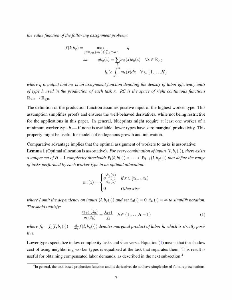
Figure 1 illustrates how differences in blueprints reflect into differences in the internal workforcecomposition of firms. The graphs at the top show the compensated labor demand integral above.The heavy, continuous line is the blueprint, which varies across graphs (becoming more intensivein high complexity tasks from left to right). The vertical dashed lines are the thresholds, whichare common for all graphs. The colored areas are the labor demand integrals. The compensatedlabor demand is shown again in the bottom row, in the form of blueprint-specific wage distributionswithin the firm (weighted by efficiency units).

If labor markets are not competitive, as in labor market model described in the next section, thresh-olds might differ across firms. Firms using different blueprints will still differ in the skill composi-tion of their internal workforce, though possibly less so than in the competitive benchmark.

The concept of firms in this model is significantly different from that in the literature on labormarket sorting (Shimer, 2005; Eeckhout and Kircher, 2011; Gautier, Teulings and van Vuuren,2010; Gautier and Teulings, 2015; Lise, Meghir and Robin, 2016; Grossman, Helpman and Kircher,2017; Lindenlaub and Postel-Vinay, 2017; de Melo, 2018; Eeckhout and Kircher, 2018). Mostmodels in this literature focus on sorting of workers to jobs (or, equivalently, to firms that employ

If one needs to evaluate output and marginal productivities as a function of labor inputs, first solve the system of Hcompensated labor demand equations (2) on q and the H−1 thresholds. Next, use equation (1) to calculate marginalproductivity gaps. Finally, use the constant returns relationship q = ∑h lh fh to normalize marginal productivities.

8

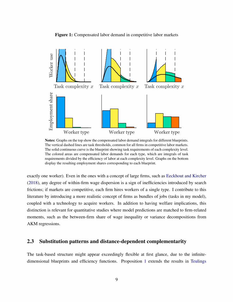
Figure 1: Compensated labor demand in competitive labor markets

Task complexity x

Wor

keruse

Worker type

Empl

oym

ent s

hare

Task complexity x

Worker type

Task complexity x

Worker type

Notes: Graphs on the top show the compensated labor demand integrals for different blueprints.The vertical dashed lines are task thresholds, common for all firms in competitive labor markets.The solid continuous curve is the blueprint showing task requirements of each complexity level.The colored areas are compensated labor demands for each type, which are integrals of taskrequirements divided by the efficiency of labor at each complexity level. Graphs on the bottomdisplay the resulting employment shares corresponding to each blueprint.

exactly one worker). Even in the ones with a concept of large firms, such as Eeckhout and Kircher(2018), any degree of within-firm wage dispersion is a sign of inefficiencies introduced by searchfrictions; if markets are competitive, each firm hires workers of a single type. I contribute to thisliterature by introducing a more realistic concept of firms as bundles of jobs (tasks in my model),coupled with a technology to acquire workers. In addition to having welfare implications, thisdistinction is relevant for quantitative studies where model predictions are matched to firm-relatedmoments, such as the between-firm share of wage inequality or variance decompositions fromAKM regressions.

2.3 Substitution patterns and distance-dependent complementarity

The task-based structure might appear exceedingly flexible at first glance, due to the infinite-dimensional blueprints and efficiency functions. Proposition 1 extends the results in Teulings

9

(2005) and shows that, on the contrary, there are strong constraints on substitution patterns.5 Lo-cally, the H×(H−1)/2 partial elasticities of complementarity or substitution depend only on factorshares and at most H−1 scalars ρh — the same number of elasticity parameters in an equally-sizednested CES structure. However, unlike with a CES, there is a straightforward way to impose furtherrestrictions on the number of parameters (both elasticities and productivity shifters for each workertype), via parametrization of blueprints and efficiency functions.Proposition 1 (Curvature of the production function). The task-based production function is con-

cave, has constant returns to scale, and is twice continuously differentiable with strictly positive

first derivatives. I denote by c = c(w,q) the cost function, use subscripts to denote derivatives

regarding input quantities or prices, and omit arguments in functions to simplify the expressions.

Then, for any pair of worker types h,h′ with h < h′:

cch,h′

chch′=

ρh

shsh′if h′ = h+1

0 otherwise(Allen partial elasticity of substitution)

f fh,h′

fh fh′=

H−1

∑h=1

ξh,h′,h1ρh

(Hicks partial elasticity of complementarity)

where ρh = bg (xh)fh

eh(xh)

[d

d xhln(

eh+1(xh)

eh(xh)

)]−1

ξh,h′,h =(

1{h≥ h+1}−∑Hk=h+1 sk

)(1{h≥ h′}−∑

hk=1 sk

)and sh =

fhlhf

=chlh

c

The curvature of the task-based production function reflects division of labor within the firm. Sup-pose that, initially, a firm only employs Alice, who belongs to the highest type H. In that case,output is linear in the quantity of labor bought from Alice. Adding another worker, Bob, of a lowertype increases Alice’s productivity, because she can now specialize in complex tasks while Bobtakes care of the simpler ones. At that point, decreasing returns to Alice’s hours reflect a reductionin those gains from specialization.

The impact of adding a third worker, Carol, on the marginal productivities of Alice and Bob de-pends on Carol’s skill level (in terms of comparative advantage), relative to Alice’s and Bob’s:

5Teulings (2005) derives elasticities of complementarity for a similar model, but using parametric efficiency func-tions and taking a limit where the number of worker types grows to infinity.

10

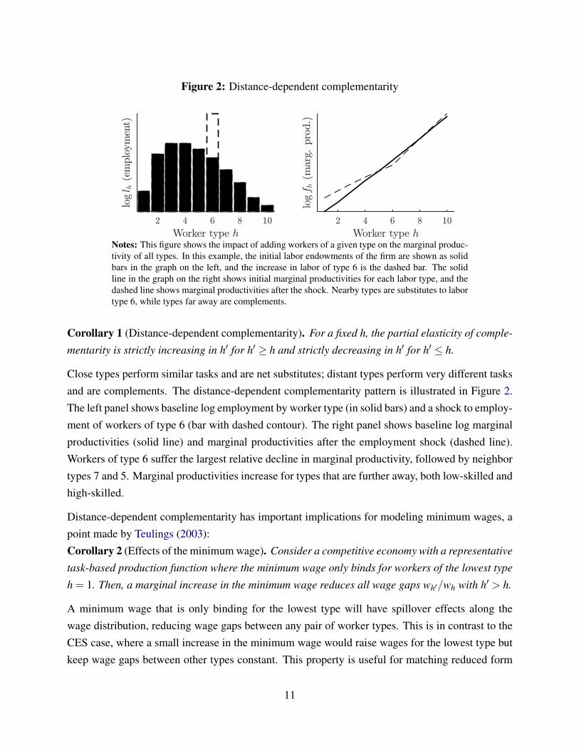
Figure 2: Distance-dependent complementarity

Worker type h2 4 6 8 10

logl h

(em

plo

ym

ent)

Worker type h2 4 6 8 10

logf h

(mar

g.pro

d.)

Notes: This figure shows the impact of adding workers of a given type on the marginal produc-tivity of all types. In this example, the initial labor endowments of the firm are shown as solidbars in the graph on the left, and the increase in labor of type 6 is the dashed bar. The solidline in the graph on the right shows initial marginal productivities for each labor type, and thedashed line shows marginal productivities after the shock. Nearby types are substitutes to labortype 6, while types far away are complements.

Corollary 1 (Distance-dependent complementarity). For a fixed h, the partial elasticity of comple-

mentarity is strictly increasing in h′ for h′ ≥ h and strictly decreasing in h′ for h′ ≤ h.

Close types perform similar tasks and are net substitutes; distant types perform very different tasksand are complements. The distance-dependent complementarity pattern is illustrated in Figure 2.The left panel shows baseline log employment by worker type (in solid bars) and a shock to employ-ment of workers of type 6 (bar with dashed contour). The right panel shows baseline log marginalproductivities (solid line) and marginal productivities after the employment shock (dashed line).Workers of type 6 suffer the largest relative decline in marginal productivity, followed by neighbortypes 7 and 5. Marginal productivities increase for types that are further away, both low-skilled andhigh-skilled.

Distance-dependent complementarity has important implications for modeling minimum wages, apoint made by Teulings (2003):Corollary 2 (Effects of the minimum wage). Consider a competitive economy with a representative

task-based production function where the minimum wage only binds for workers of the lowest type

h = 1. Then, a marginal increase in the minimum wage reduces all wage gaps wh′/wh with h′ > h.

A minimum wage that is only binding for the lowest type will have spillover effects along thewage distribution, reducing wage gaps between any pair of worker types. This is in contrast to theCES case, where a small increase in the minimum wage would raise wages for the lowest type butkeep wage gaps between other types constant. This property is useful for matching reduced form

11

estimates of minimum wage spillovers (see Figure 7).

2.4 Parametric example

Consider the following parametrization, which I use in the quantitative exercises of this paper:Example 1 (Exponential-Gamma parametrization).

eh(x) = exp(αhx) −1 = α1 < α2 < · · ·< αH−1 < αH = 0

bg(x) =xkg−1

zgΓ(kg)θkgg

exp(− x

θg

)(zg,θg,kg) ∈ R3

>0

The exponential function is a straightforward way to generate log-supermodularity and is used inother models of comparative advantage (e.g. Krugman (1985); Teulings (1995)). Differences in theαh coefficients determine the degree of comparative advantage between any two worker types. Theexpression for blueprints is the probability density function of a Gamma distribution divided by a"productivity" term zg. Doubling zg divides the quantity of tasks needed per unit of output by two,effectively doubling physical productivity.

Appendix B presents the mapping between marginal productivity gaps and task thresholds in thisparametrization, as well as formulas for compensated labor demand integrals in terms of incom-plete Gamma functions. These formulas are useful because they dispense with numerical integra-tion, improving computational performance. Incomplete Gamma functions are readily available insoftware packages commonly used by economists.

The parameter θg is related to average task complexity. All else equal, firms with higher θg re-quire more complex tasks and employ more skilled workers (in terms of comparative advantage).Increases in task complexity over time, modeled as changes in θg, provide an intuitive way tomodel skill-biased technical change because higher complexity is linked to increasing returns toskill (measured as the worker group h). The shape parameter kg determines the dispersion of tasks.If two firms differ only in this parameter, the one with the smallest kg has fatter tails. Thus, differ-ences in kg in the cross-section translate into some firms being more specialized than others in theirhiring patterns.

This approach allows for modeling firm-level differences in skill intensity, skill dispersion, and pro-ductivity with a small number of parameters, while ensuring sensible substitution patterns withinall firms. To understand the economic content behind those parametric restrictions, consider an

12

example of two firms in the retail sector. One, with a low θg, is a small local shop, while the other,with a high θg, is a large online retailer. In the first one, most tasks are of low complexity, measuredin terms of how they benefit from schooling: stocking shelves, operating the register, and cleaning.In those tasks, workers with little formal education can substitute for others with a college degree.Because workers with a college degree cost much more, that first firm mostly hires less educatedworkers. In contrast, the online retailer is intensive in tasks such as web design, system administra-tion, and business analytics, where college-graduated workers usually perform much better. This iswhy those firms find it profitable to use a more skilled workforce.

3 Markets and wages

This section builds a labor market model with monopsonistic firms and free entry. The first sub-section lays out the structure of the economy. The second subsection describes the functioning oflabor markets, solves the problem of the firm, and shows an important property of the model: goodsencapsulate firm heterogeneity in skill intensity and wages. The third subsection derives analyticalresults on what determines wage differentials between firms and how the wage distribution changesover time.

This is the point of departure from other task-based assignment models of comparative advan-tage such as Teulings (2005), Costinot and Vogel (2010), and Acemoglu and Autor (2011). Thecontributions of the previous section fit inside that literature: new formulas for elasticities of com-plementarity and substitution, along with the convenient exponential-gamma parametrization. Thissection introduces more significant deviations. First, aggregate demand for tasks is CES in all pa-pers in that literature, but not in this model. This has implications for comparative statics. Forexample, the introduction of a minimum wage always decreases wage gaps in Teulings (2000), buthere the same shock might cause wage polarization. Second, labor markets are not competitive.And third, workers in this model differ not only in comparative advantage but also in absoluteadvantage, generating realistic distributions of log wages that include bunching at the minimumwage.

3.1 Factors, goods, technology, and preferences

Consider an economy with N = {N1, . . . ,NH} workers of each type h, and a large number ofentrepreneurs. Entrepreneurs own entrepreneurial talent, whose total stock in the economy is T

13

and which is used to create firms. The model is static.

There are G final goods in this economy, interpreted as differentiated varieties within an industry.6

An entrepreneur j may set up a firm producing one good g ∈ {1, . . . ,G} or not enter at all. Settingup a firm requires a fixed cost Fg, paid in units of entrepreneurial talent. Once that cost is paid,the entrepreneur receives the blueprint bg and a random draw of workplace amenities a j from agood-specific distribution with strictly positive support and a finite mean ag. The role of workplaceamenities will be explained below. Hiring and production decisions are done after the amenitiesdraw is observed, as discussed in the next subsection.

I assume that there is a competitive market for entrepreneurial talent and that entrepreneurs canform coalitions to insure against idiosyncratic risk associated with the draw of firm amenities a j.These assumptions allow me to abstract from the distribution of entrepreneurial talent and to pindown firm entry by equating expected profit and entry costs for each good g:

Ea j|g[πg(a j)

]= Fg pT = Fg ∀g

where πg(a j), defined below, denotes profits achieved by a firm with amenities a j producing goodg. The second equality follows from assuming that entrepreneurial talent is the numeraire in thiseconomy. This choice of numeraire is valid because firms have positive profits, as I will showbelow, and so the price of entrepreneurial talent cannot be zero. A positive price for entrepreneurialtalent also implies that all of it is used up in equilibrium:

∑g

JgFg = T (3)

where Jg is total entry of firms producing good g. When there is a single good g= 1 in this economy,the number of firms is fixed at J1 = T/F1. But with multiple goods, the number of firms producingeach good might respond to shocks.

The utility function of entrepreneurs, UE , is a constant elasticity aggregator of consumption Q1, . . . ,QG.Preferences of worker i of type h, captured by UL

hi, depend on both consumption and the firm j

6This is my preferred interpretation because, in many contexts, changes in inequality happen within industries (seee.g. Card, Heining and Kline (2013) and Song et al. (2018)). Consistent with this interpretation, the next section showsthat the estimated elasticity of substitution for the two goods in the quantitative exercise is large. The model can alsobe used for studying between-industry phenomena, such as between-industry sorting in Abowd et al. (2018).

14

where she is employed:

UE({

Qg}G

g=1

)=C

({Qg}G

g=1

)UL

hi

({Qg}G

g=1 , j)=C

({Qg}G

g=1

)[a j exp

(ηi j)] 1

βh

where C({

Qg}G

g=1

)=

[G

∑g=1

Qgσ−1

σ

] σ

1−σ

and ηi j ∼ Extreme Value Type I

Firms matter to workers not only due to their overall level of amenities a j, but also because of anidiosyncratic component ηi j. This component captures match-specific features such as distanceto the workplace or personal relationships with the manager or other coworkers. The parametersβh measure the importance of consumption relative to these non-pecuniary elements. Higher βh

implies that the market for labor of type h is more competitive. The details of the labor market arediscussed in the next subsection.

Markets for goods are competitive. Thus, any equilibrium will feature prices pg equal to the

marginal cost of good g at all firms producing that good. There is a price index P=[∑

Gg=1 p1−σ

g

] 11−σ

such that consumption level C costs C×P. Because C(·) is homothetic, aggregate consumption isonly a function of prices and aggregate income.

Continuing with the example from Section 2.4, the small local shop and the large online retailer areinterpreted as differentiated varieties in the retail sector, with elasticity of substitution σ . In addi-tion to task requirements, these firms might differ in entry costs and the average level of amenities.The online retailer might require substantial capital investment or managerial input to set up, jus-tifying high entry costs Fg. If ag is higher for the large retailers, then they are also more desirableworkplaces on average.

3.2 Labor markets, the problem of the firm, and equilibrium

Labor markets are based on the model of Card et al. (2018), where firms compete monopsonisticallyfor labor. Each worker is characterized by its type h ∈ {1, . . . ,H} and a quantity of efficiency unitsof labor ε . The distribution of efficiency units of labor across workers of type h is continuous with

15

density rh(·) and support over the real line.7 Throughout this section, it is important to distinguishbetween quantities of workers, denoted by n, and quantities of labor, denoted by l. Worker earningsare denoted by y, while prices for labor are denoted by w.

Labor regulations prevent firms from paying a total compensation of less than¯y to any worker.

I refer to¯y as the minimum wage; the model has no variation in hours worked, so earnings and

wages are interchangeable. Workers with low ε might have a marginal product of labor lesserthan

¯y at some firms, in which case hiring those workers would be unprofitable. Thus, I allow

firms to reject workers with productivity below some minimum value¯εh j, generating involuntary

non-employment.

3.2.1 Firm-level labor supply and labor costs

There are separate labor markets for each worker group h. The timing of each of these labor marketsis as follows:

1. Each firm j posts a price per labor efficiency unit wh j and a rejection cutoff¯εh j.

2. Workers observe all wh j and¯εh j. Based on that information, they choose firms that maximize

their indirect utility. If no firm is chosen, the worker earns zero income.

3. Firms observe (h,ε) of workers who applied to them (but not idiosyncratic preference shiftersηi j) and hire those with ε >

¯εh j.

4. Production occurs and hired workers are paid y = max{wh jε,¯y}. Rejected workers, if any,

earn zero income.

To study worker choices in step 2, consider the indirect utility of a worker i characterized by (h,ε),if this worker chooses firm j:

Vih(ε, j) =1{

ε ≥¯εh j}

max{

εwh j,¯y}

P︸ ︷︷ ︸Consumption

[a j exp

(ηi j)] 1

βh

=

1P

exp(

βh log(max

{εwh j,

¯y})

+ loga j +ηi j

) 1βh if ε ≥

¯εh j

0 otherwise

7I employ LogNormal distributions of ε in the quantitative exercise. Counterfactual exercises require a parametricassumption for rh(·), which is used to obtain the number of workers driven to unemployment because of the minimumwage and the distribution of ε in that unobserved population.

16

where the indicator function denotes that worker i earns positive income at firm j only if i’s endow-ment of labor efficiency units is at least

¯εh j.

Because ηi j is drawn from a Type I Extreme Value distribution, the probability of a worker (h,ε)choosing a particular firm j is given by:

P

(j = argmax

j′∈{1,...,J}Vih(ε, j′)

)= 1

{ε >

¯εh j}

a j

(max

{εwh j,

¯y}

ωh(ε)

)βh

where ωh(ε) =

(∑j′

1{

ε >¯εh j′}

a j′max{

εwh j′,¯y}βh

) 1βh

The "inclusive value" ωh(ε) is a measure of demand for skills in this model. A high value meansthat many firms are posting high wages for type h and willing to hire that particular ε , despite theminimum wage. That makes those workers harder to attract for any individual firm because theyhave good outside options at other firms. Mechanically, ωh(ε) has an allocative role similar to thatof wages in competitive models: it is a cost shifter that firms take as given and that ensures labormarket clearing.

The number of workers choosing a particular firm and the resulting supply of labor are increasingfunctions of posted wages, conditional on rejection cutoffs:

nh(wh j, ¯εh j,a j) = Nha j

∫∞

¯εh j

(max

{εwh j,

¯y}

ωh(ε)

)βh

rh(ε)dε (4)

lh(wh j, ¯εh j,a j) = Nha j

∫∞

¯εh j

exp(ε)

(max

{εwh j,

¯y}

ωh(ε)

)βh

rh(ε)dε (5)

Finally, total labor costs are given by:

Ch(wh j, ¯εh j,a j) = Nha j

[∫ ¯y

wh j

¯εh j

¯yβh+1

ωh(ε)βhrh(ε)dε +

∫∞

¯y

wh j

(εwh j

)βh+1

ωh(ε)βhrh(ε)dε

](6)

In these expressions, I omit the dependency of ωh(ε) on the own firm’s posted wage wh j because,with monopsonistic competition, ωh(ε) is taken as given by firms.

17

3.2.2 Problem of the firm

Firms maximize profit by choosing posted wages and rejection cutoffs:

πg(a j) = maxw j,¯ε j

pg f(l(w j, ¯

ε j,a j),bg)−

H

∑h=1

Ch(wh j, ¯εh j,a j)

The following Lemma shows that this problem has intuitive solutions and that the model admits arepresentative firm for each good:Lemma 2. The solution of the problem of the firm is interior and characterized by the following

first order conditions:

pg fh(l(w j, ¯

ε j,a j),bg) βh

βh +1=wh j h = 1, . . . ,H (7)

pg fh(l(w j, ¯

ε j,a j),bg)

¯εh j =

¯y h = 1, . . . ,H (8)

Additionally, firms producing good g choose the same wages wg and rejection criteria¯εg. Output

and employment are linear in firm amenities: q j =a jag

qg and l j =a jaglg, where qg and lg denotes

mean output and mean labor demand for all firms producing good g, respectively.

The first order conditions represent trade-offs along two different margins: workers above the min-imum wage and workers around the rejection threshold. To build intuition on the optimality condi-tion on wages, denote by l+h j the sum of efficiency units at firm j supplied by workers earning morethan the minimum wage. A proportional increase in posted wages d logwh j brings in (βd logwh j)l+h j

labor units, generating (βd logwh j)l+h j pg fh(·) in additional revenues. Labor costs increase for tworeasons. First, the firm pays (βd logwh j)l+h jwh j for the additional labor purchased. Second, a higherwage increases the wage bill for current workers by d logwh jl+h jwh. Setting added revenues equalto additional costs yields Equation 7.

Equation 8 is the first order condition on the rejection cutoffs. A lower cutoff brings in additionalworkers with ε =

¯εh j, each of which increases revenues by pg fh¯

εh j. When firms chose thresholdsoptimally, that additional revenue equals the minimum wage

¯y, which is the cost of labor at that

margin.

Figure 3 illustrates how workers are divided in three groups according to their level of efficiencyunits. Those to the left of

¯εh j are rejected. Those with ε >

¯y/wh j earn the wage posted by the

firm times their quantity of labor units. Finally, those in the intermediate range earn the minimum

18

Figure 3: Choice of rejection criterion and bunching at the minimum wage

Notes: This figure shows thresholds in the distribution of efficiencyunits of labor ε that determine whether worker are rejected by firm j,are employed receiving the minimum wage, or employed receiving theposted wage times the number of efficiency units. The horizontal axisis in log scale. The blue line shows the distribution of efficiency units,which is LogNormal in this illustration (as well as in the quantitativeexercise). When there is a single good in the economy, such that thereis a representative firm, the distribution of log wages for workers oftype h is a truncated normal with a peak at the minimum wage. Themass of this peak is given by the area between the two vertical lines inthis graph.

wage. The first order conditions imply that these two thresholds are proportional to each otherin all firms choosing labor inputs optimally, with their ratio being given by 1+ 1/βh. Log wagehistograms simulated from the model have peaks at the minimum wage corresponding to the massof workers between the two vertical lines. Bunching at the minimum wage is often observed inthe data (DiNardo, Fortin and Lemieux, 1996; Harasztosi and Lindner, 2018) but is not a commonfeature in models of wage inequality.

Lemma 2 also shows that firms producing the same good are equal in wages and input intensities.Dispersion in amenities within good only scales the firm up or down. This result simplifies theanalysis of between-firm wage differentials and sorting in this model by restricting the sources ofthese patterns to differences in blueprints, entry costs, or mean amenities ag. It also simplifies the

19

expression for ω(ε), making the computation of labor demands feasible:

ωh(ε) =

(∑g

Jg1{

ε >¯εhg}

ag max{

εwhg,¯y}βh

) 1βh

(9)

3.2.3 Equilibrium

An equilibrium of this model is a set of prices {pg}Gg=1, aggregate consumption {Qg}G

g=1, firm entry{Jg}G

g=1, and choices by representative firms {wg, ¯εg}G

g=1 such that:

1. Markets for goods clear:

Qg =[ pg

P

]−σ IP= Jgqg ∀g (10)

where I = T +G

∑g=1

Jg

H

∑h=1

Ch(whg, ¯εhg, ag)

2. For all g, firm choices solve the set of equations (7) and (8).

3. Entrepreneurs have zero ex-ante expected profits:

Ea j|g[πg(a j)

]= pg f (l(wg, ¯

εg, ag),bg)−H

∑h=1

Ch(whg, ¯εhg, ag) = Fg ∀g (11)

4. The market for entrepreneurial talent clears (Equation 3).

Labor market clearing is implied by the definition of ωh(ε), which ensures that the number of jobapplicants to all firms (calculated using Equation 4) is equal to total number of workers Nh.

Solving for equilibrium can seem challenging at first glance. Using a convenient set of choicevariables reduces the problem to solving a square system of (H + 1)×G equations where thechoice variables are firm-specific task thresholds, firm-level output, and prices for each good. Theprocedure below describes how to calculate that system of equations:

1. Start with values for mean output qg and task thresholds xg = {x1g, . . . , xHg} for the repre-sentative firms of each type, along with prices for goods pg.

2. Use the compensated labor demand integral for the task-based production function to findaverage labor demands lhg (Equation 2 in the text, or Equation 15 in Appendix B if using the

20

exponential-Gamma parametrization).

3. Find marginal products of labor fhg via the non-arbitrage conditions (1) and the constantreturns to scale relationship ∑h fhglhg = qg.

4. Employ the first order conditions of the firm (7) and (8) to find wages whg and rejectioncutoffs

¯εhg, respectively.

5. Calculate relative consumption Qg/Q1 =(pg/p1)−σ and relative firm entry Jg/J1 =(Qg/Q1)/(qg/q1).

6. Pin down entry of firm type 1 (and thus all others) with entrepreneurial talent clearing: J1 =

T/(∑g FgJg/J1).

7. Obtain ωh(ε) using expression 9.

8. Calculate the error in the system of equations, which has two components:

(a) The deviation between lhg found in step 2 and that implied by the labor supply curve (5).

(b) The deviation between profits and entry costs in Equation 11.

That system of equations can be solved using standard numerical procedures, with the restrictionsthat qg > 0, pg > 0, and 0 ≤ x1g ≤ x2g ≤ ·· · ≤ xHg ∀g. These restrictions can be imposed throughtransformations of the choice variables: log prices, log quantities, log of the lowest task thresholdsx1g, and log of differences between consecutive thresholds xhg− xh−1,g for h = 2, . . . ,H−1.

3.3 Determinants of the wage distribution

The key outcome of the analysis is how wages differ between groups, within groups, and acrossfirms. We know from the labor market structure that log earnings of a worker i of type h at afirm producing good g take the form logyihg = max{logwhg + logεi, log

¯y}. Variation in wages

between worker groups is driven by differences in whg. Within-group variation of log wages hasthree components: the dispersion of efficiency units, differences in mean log wages across goodsfor the same worker type, and censoring by the minimum wage.

The following proposition provides intuition about how wages vary across firms producing differentgoods:Proposition 2. 1. If bg(x) = b(x)/zg and Fg

agis common across goods, then there are no firm-

level wage premia:

logyihg = max{

λh + logεi, log¯y}

21

for scalars λ1, . . . ,λH .

2. If there is no minimum wage (¯y= 0), βh = β , and bg(x)= b(x)/zg, then wages are log additive

in worker type and firm type:

logyihg = λh +1

1+βlog(

Fg

ag

)+ logεi

3. If there is no minimum wage, βh = β , and there are firm types g, g′ and worker types h′ h

such that `h′g′/`hg′ > `h′g/`hg (that is, good g′ is relatively more intensive in h′), then:

yih′g′/yihg′ > yih′g/yihg

The first part of Proposition 2 shows that wage dispersion for similar workers exists only if thereare differences in the shapes of blueprints (such that firms differ in skill intensity) or in the ratio ofentry costs to mean amenities. Notably, differences in physical productivity across goods (denotedby zg above) are not enough to generate wage differentials between firms. The reason is that, ifthe ratio of entry costs to firm amenities is the same, differences in physical productivity lead toadditional entry and reduced marginal utility of consumption for the good with more productivity,up to the point where marginal revenue product of labor is equalized across firms.

The second part highlights the role of entry costs in generating wage differences across firms. Thezero profits condition implies that firms producing goods with higher entry costs need to operate atlarger scale. To hire more workers, these firms need to post higher wages, unless the differences inentry costs are exactly offset by differences in mean amenities.

The third part of Proposition 2 shows how heterogeneity in skill intensity generates differentialwage gaps across firms. Firms using some factors more intensively than others must pay a relativepremium to that factor. Thus, in general, the model cannot generate log-additive wages as inAbowd, Kramarz and Margolis (1999), except when factor intensities do not vary. Equal skillintensities are ensured by the conditions imposed in (2).

The inability of this model to generate log-additive wages and sorting simultaneously echoes someresults in the literature on labor market sorting, such as those in Eeckhout and Kircher (2011). Butit is possible that skill-intensive firms pay a positive wage premium for all worker types if thosefirms have high entry costs relative to amenities. The quantitative exercise shows that this flexibilityis necessary for fitting the data.

22

To provide a concrete example of how firms differ in equilibrium, consider the Exponential-Gammaparametrization introduced in Subsection 2.4. Under that parametrization, goods are fully describedby five scalars: blueprint complexity θg, blueprint shape kg, blueprint productivity zg, mean ameni-ties ag, and the ratio of entry costs to mean amenities Fg/ag. These scalars map directly into fiveempirical measures for the set of firms producing that good, respectively: mean worker education,dispersion in worker education, share of total workforce employed by those firms, mean firm size,and firm-level wage premia.

The next step in the analysis is understanding how the wage distribution changes over time, givenshocks to labor supply, labor demand, and minimum wages. As a starting point, the followingproposition considers a case in which the supply of skill, demand for task complexity, and minimumwages rise in tandem:Proposition 3 (Race between technology, education, and minimum wages). Start with a baseline

economy characterized by parameters({eh,Nh,βh}H

h=1 ,{

bg,Fg, ag}G

g=1 ,T,σ ,¯y)

and consider a

new set of parameters denoted with prime symbols. Assume eh are decreasing functions to simplify

interpretation (more complex tasks are harder to produce). Let ∆0, ∆1 and ∆2 denote arbitrary

positive numbers and consider the following conditions:

1. N′h = ∆0Nh ∀h and T ′ = ∆0T : The relative supply of factors remains constant.

2. e′h(x) = eh

(x

1+∆1

)∀h: Workers become better at all tasks and the degree of comparative

advantage becomes smaller for the current set of tasks (e.g. both high school graduates and

college graduates improve at using text editing software, but the improvement is larger for

high school graduates).

3. b′g(x) =1

(1+∆1)(1+∆2)bg

(x

1+∆1

)∀g: Production requires fewer tasks, but the composition of

tasks moves towards increased complexity.

4.¯y′ =

¯y: The minimum wage stays constant relative to the price of entrepreneurial talent.

If these conditions are satisfied, the equilibrium under the new parameter set is identical to the

initial equilibrium, except that prices for goods are uniformly lower: p′g = pg/(1+∆2) and P′ =

P/(1+∆2).8

Proposition 3 delineates technological progress in this economy. Production becomes more ef-ficient by using tasks that are more complex. At the same time, the skill of workers increase,changing the set of tasks where skill differences are relevant. If minimum wages remain as impor-

8Using the exponential-gamma parametrization, changes in comparative advantage functions and blueprints areequivalent to α ′h = αh/(1+∆1), θ ′g = (1+∆1)θg, k′g = kg, and z′g = (1+∆2)zg.

23

tant, then there is a uniform increase in living standards. Wage differences between worker groupsand between firms for the same group remain stable.

If these transformations are not balanced, then relative prices and the allocation of resources mightchange. The overall effect on the wage distribution and sorting is difficult to study analyticallybecause they interact through four different channels: (i) changes in the economy-wide measuresof skill scarcity, ωh(·); (ii) changes in relative consumption, which are tantamount to changes inthe distribution of firm types; (ii) changes in the employment composition of each firm, conditionalon type; and (iv) changes in firm-specific wage premia. Since all of these channels are potentiallyimportant, the best way to disentangle the role of each shock is through a quantitative applicationof the model.

It is possible, however, to obtain some intuition about how firm heterogeneity might amplify orattenuate the impact of specific shocks on the wage distribution, relative to a framework with arepresentative firm. Shocks that affect the price for skills will have differential effects on the costof goods that are produced using different sets of tasks. Those changes in cost are passed throughto consumers. As they substitute towards cheaper goods, the aggregate set of tasks being producedby this economy shifts towards more or less complex tasks. That shift acts as a secondary demandshock, leading to further adjustments in the price for skills.

The following proposition isolates the effect of that secondary shock by considering what happenswhen there is a change in cost for a particular firm, in a simplified version of the model:Proposition 4 (Changes in relative output affects the returns to skill). Consider a competitive ver-

sion of this economy (βh = ∞, Fg = 0) with two goods (G = 2), no minimum wages (¯y = −∞),

and where relative labor demand Q2/Q1 is an exogenous parameter rather than the outcome of

consumer optimization. Assume good g = 2 is relatively more intensive in high-complexity tasks,

such that b2(x)/b1(x) is increasing. Then, an increase in Q2/Q1 causes increases in wage gaps

wh+1/wh.

The full effect of a shock to labor supply, technical change, or minimum wages combines a directeffect and this secondary demand effect. Consider for example a minimum wage hike. As discussedin the presentation of the task-based production function, minimum wages decrease all wage gapsin this economy when there is a representative firm. But with two firms, minimum wages increasethe cost of the low-skill good relative to the high-skill good. The secondary demand shock is inthe direction of increased wage inequality, as in Proposition 4 above. The overall effect can beeither an attenuated decline in wage gaps or wage polarization, whereby wages increase for lowand high worker groups relative to intermediate groups. The next section of this paper shows that

24

this channel can be quantitatively important and help fit reduced-form estimates of the effects ofminimum wage shocks.

Proposition 4 is conceptually related to papers where structural shocks change the compositionof jobs in the economy, causing additional effects on the wage distribution through this channel.Examples of such papers are Kremer and Maskin (1996), Acemoglu (1999), and Mak and Siow(2018), which study supply shocks; Acemoglu and Restrepo (2018), which studies automation;Acemoglu (2001), which studies minimum wages; and Sampson (2014) and Davis and Harrigan(2011), which study trade liberalization.

4 Quantitative exercise: wage inequality and sorting in Rio Grandedo Sul, Brazil

While the literature covering countries such as the US and Germany often tries to explain increasingwage disparities in recent decades, the academic debate in Brazil attempts to rationalize a declinein inequality starting in the 1990s. The most salient facts in the Brazilian context are significantincreases in both the minimum wage and educational achievement, following policies aimed at uni-versal primary schooling in the 1980s and 1990s and expansion in access to college-level educationin the 2000s. In this section, I study the Brazilian context as a proof of concept for the model. Inthe first step of the analysis, I take a sparsely parameterized, over-identified version of the model tothe data and study whether it can rationalize changes from 1998 through 2012. In the second step,I use the estimated model to generate counterfactuals that isolate the individual impact of supply,demand, and minimum wages.

Throughout the analysis, I restrict my attention to the formal sector in the southernmost state ofBrazil, Rio Grande do Sul. Similarly to many other developing countries, a substantial share ofthe Brazilian workforce is informal (employed at firms that evade regulations such as payroll taxesand minimum wages). It would be ideal to include formal and informal workers in the analysisbecause the model has general equilibrium effects. That is impossible, however, for data limita-tions. Households surveys measure employment and wages in the informal sector, but I requirematched employer-employee data to gauge between-firm wage dispersion for similar workers andlabor market assortativeness.

To partially address problems related to informality, I restrict my analysis to Rio Grande do Sul,the largest state in Southern Brazil. Except for the Southeast, the Brazilian South is the region with

25

the lowest rates of employment informality in the country. The Southeast is less interesting forthis exercise, however, because higher wages in that region make the minimum wage shock lessrelevant.9 I discuss the implications of ignoring the informal sector before presenting the results ofthe counterfactual exercises. In addition, Appendix C.2 contains a thorough analysis of inequalityand education patterns using a different data source that includes the informal sector.

The data source used in this section is the RAIS (Relação Anual de Informações Sociais), a confi-dential matched employer-employee dataset administered by the Brazilian Ministry of Labor. Firmsare mandated by law to report to RAIS, and in doing so provide information about their employees.The dataset I utilized contains information about both the firm (including legal status, economicsector, and the municipality in which it is registered) and each worker it formally employs (includ-ing education, age, earnings in December, contract hours, and hiring and separation dates).

Because I am interested in equilibrium effects, the sample I use has few restrictions. I select adultsof both genders between 18 and 54 years of age, who are not currently in school, and who areworking in December having been hired in November or earlier. I only consider one job per workerper year. The resulting data set has 1,494,186 workers and 148,203 firms in 1998, and 2,398,391workers and 238,545 firms in 2012. For each worker, I calculate the hourly wage based on theirmonthly earnings and contract hours, before winsorizing the bottom and top percentiles of the wagedistribution. Summary statistics are provided in Table 6, located in Appendix C.1.

4.1 Target moments

Figure 4 demonstrates the evolution of wages in the Rio-Grandense economy. The top left panelshows that, from 1998 to 2012, real wages have increased for all deciles of the log wage distri-bution, and particularly so for the lowest deciles. Almost all commonly used measures show areduction in inequality: upper-tail or lower-tail percentile gaps (top-right panel), differences inmean log wage between workers with secondary education (that is, those complete high-schooland college dropouts) and less educated workers, and the variance of log wages — for the sampleas a whole and within each educational group. The single exception is the gap between secondaryand tertiary education (workers that had completed college and beyond), which rose until 2006 andsubsequently remained stable through to the end of the period studied. In Appendix C.2, I showthat wage inequality trends are similar in a different data set that includes informal workers.

9I use a single state in the South because the estimator of variance components of Kline, Saggio and Sølvsten(2018) performs better in well-connected labor markets (in terms of worker transitions between firms). Table 5 showsthat the sample size is large enough to generate precise estimates.

26

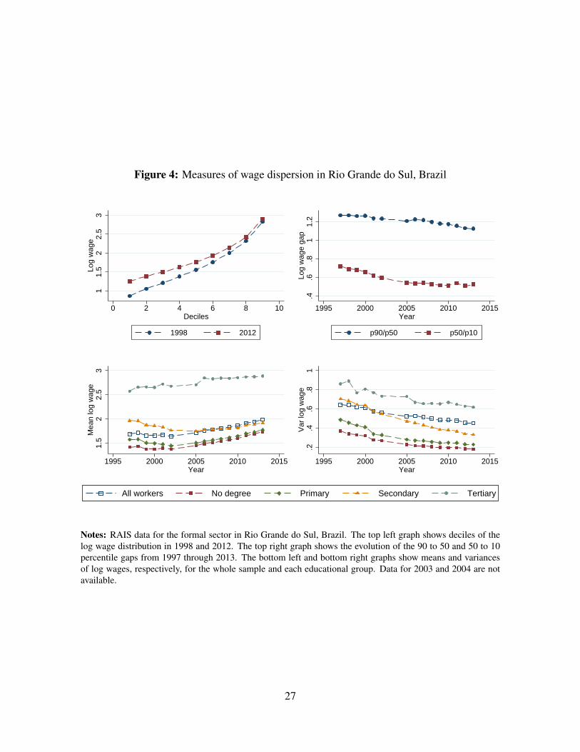
Figure 4: Measures of wage dispersion in Rio Grande do Sul, Brazil

11.

52

2.5

3Lo

g w

age

0 2 4 6 8 10Deciles

1998 2012

.4.6

.81

1.2

Log

wag

e ga

p1995 2000 2005 2010 2015

Year

p90/p50 p50/p10

1.5

22.

53

Mea

n lo

g w

age

1995 2000 2005 2010 2015Year

.2.4

.6.8

1V

ar lo

g w

age

1995 2000 2005 2010 2015Year

All workers No degree Primary Secondary Tertiary

Notes: RAIS data for the formal sector in Rio Grande do Sul, Brazil. The top left graph shows deciles of thelog wage distribution in 1998 and 2012. The top right graph shows the evolution of the 90 to 50 and 50 to 10percentile gaps from 1997 through 2013. The bottom left and bottom right graphs show means and variancesof log wages, respectively, for the whole sample and each educational group. Data for 2003 and 2004 are notavailable.

27

Figure 5: Changes in educational achievement and minimum wages

.1.2

.3.4

.5S

hare

of h

ours

wor

ked

1995 2000 2005 2010 2015Year

No degreePrimary

Secondary Tertiary

-1.2

-1.1

-1-.

9-.

8-.

7Lo

g m

in. w

age/

med

ian

wag

e

.2.4

.6.8

1Lo

g re

al m

in. w

age

1995 2000 2005 2010 2015Year

Real

Relative

Notes: RAIS data for the formal sector in Rio Grande do Sul, Brazil. The top graph shows, foreach year from 1997 through 2012, the share of hours worked by employees in each educationalgroup. The bottom graph shows the evolution of minimum wages in the same years, both in realterms and relative to the median wage in that year. Data for 2003 and 2004 are not available.

The estimation procedure will target levels from 1998 and changes from 1998-2012 in between-group mean log wage gaps and in the variance of log wages within each group.

The literature studying wage inequality in Brazil highlights two candidate explanations for thesepatterns: increased educational achievement and minimum wages. Figure 5 shows that both factorsare relevant in Rio Grande do Sul. The first graph displays the fraction of hours worked by employ-ees in each educational group. The pattern is striking: workers with less than a complete primaryeducation (that is, less than eight years of schooling) supply 40 percent of the hours in 1998, butonly around 15 percent in 2012. On the other hand, the group with a complete secondary education(high school and college dropouts) increased its participation level by almost 30 percentage points.Moreover there is a substantial increase in college completion in relative terms (from 9.4 percentto 12.2 percent), though they remain a fraction of the formal workforce.

In a strict sense, these are not changes in the supply of labor, but are instead the observed employ-

28

ment shares for each educational group. Even with the exogenous labor supply in the model, thesetwo concepts differ because the minimum wage creates involuntary non-employment. Figure 11 inAppendix C.2 shows similar trends in the share of all adults belonging to each of these educationalgroups, regardless of whether they participate in the labor force or not. That fact indicates that thesource of changes in schooling achievement of the workforce are changes in the education levelsfor the whole population, not changes in selection patterns into employment.

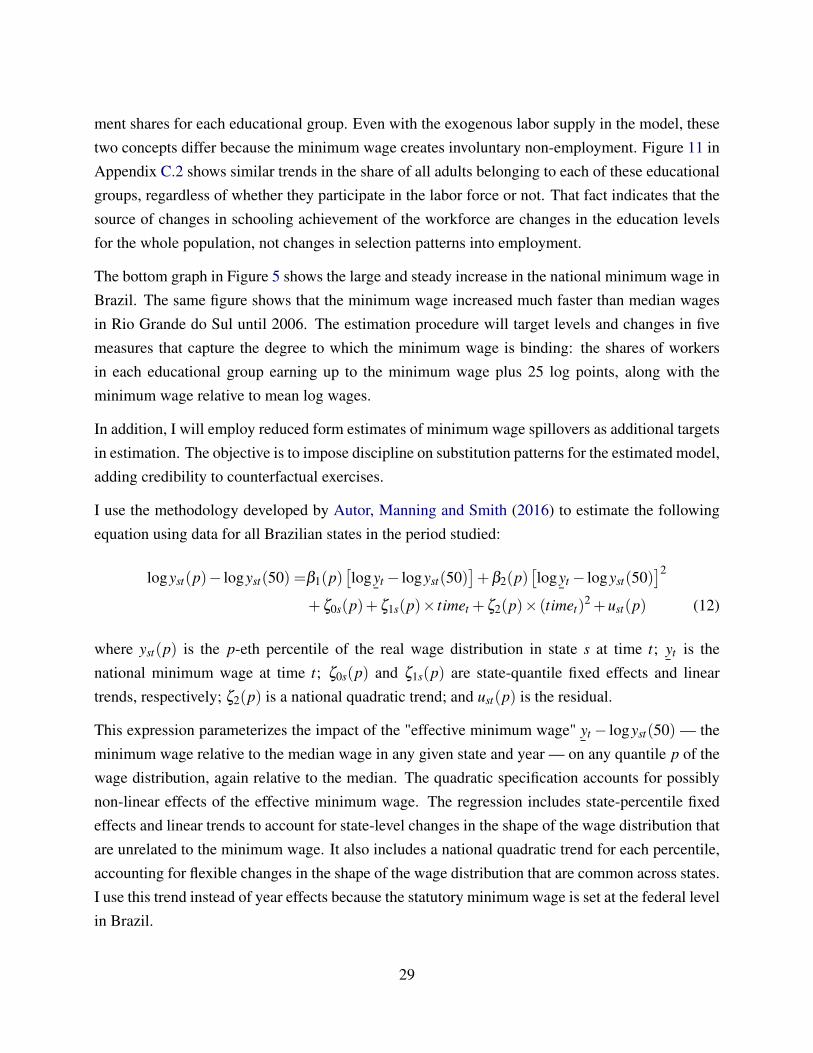
The bottom graph in Figure 5 shows the large and steady increase in the national minimum wage inBrazil. The same figure shows that the minimum wage increased much faster than median wagesin Rio Grande do Sul until 2006. The estimation procedure will target levels and changes in fivemeasures that capture the degree to which the minimum wage is binding: the shares of workersin each educational group earning up to the minimum wage plus 25 log points, along with theminimum wage relative to mean log wages.

In addition, I will employ reduced form estimates of minimum wage spillovers as additional targetsin estimation. The objective is to impose discipline on substitution patterns for the estimated model,adding credibility to counterfactual exercises.

I use the methodology developed by Autor, Manning and Smith (2016) to estimate the followingequation using data for all Brazilian states in the period studied:

logyst(p)− logyst(50) =β1(p)[log

¯yt− logyst(50)

]+β2(p)

[log

¯yt− logyst(50)

]2+ζ0s(p)+ζ1s(p)× timet +ζ2(p)× (timet)

2 +ust(p) (12)

where yst(p) is the p-eth percentile of the real wage distribution in state s at time t;¯yt is the

national minimum wage at time t; ζ0s(p) and ζ1s(p) are state-quantile fixed effects and lineartrends, respectively; ζ2(p) is a national quadratic trend; and ust(p) is the residual.

This expression parameterizes the impact of the "effective minimum wage"¯yt − logyst(50) — the

minimum wage relative to the median wage in any given state and year — on any quantile p of thewage distribution, again relative to the median. The quadratic specification accounts for possiblynon-linear effects of the effective minimum wage. The regression includes state-percentile fixedeffects and linear trends to account for state-level changes in the shape of the wage distribution thatare unrelated to the minimum wage. It also includes a national quadratic trend for each percentile,accounting for flexible changes in the shape of the wage distribution that are common across states.I use this trend instead of year effects because the statutory minimum wage is set at the federal levelin Brazil.

29

Table 1: Reduced form estimates of minimum wage spillovers

QuantileLevels Differences

OLS IV OLS IV

100.584 0.427 0.641 0.540

(0.062) (0.068) (0.050) (0.052)

200.369 0.246 0.389 0.321

(0.049) (0.043) (0.036) (0.029)

300.204 0.158 0.241 0.167

(0.073) (0.054) (0.034) (0.022)

400.106 0.025 0.119 0.052

(0.032) (0.031) (0.029) (0.023)

60-0.051 0.044 -0.084 -0.019(0.037) (0.029) (0.041) (0.024)

700.091 0.259 -0.037 0.067

(0.095) (0.060) (0.059) (0.053)

800.113 0.281 0.015 0.028

(0.108) (0.088) (0.079) (0.063)

900.230 0.282 0.113 -0.011

(0.085) (0.093) (0.073) (0.068)N 378 378 351 351Cragg-Donald F 11.50 43.24

Notes: Each cell in this table corresponds to the marginal effects of the "effec-tive minimum wage" (log statutory minimum wage minus median log wage) onquantiles of the wage distribution relative to the median log wage, coming fromseparate (quantile-specific) regressions. Each observation is a state-year and theregression is weighted by total hours worked. All years from 1996 through 2013are included except 2002, 2003, 2004 and 2010, years in which data is not avail-able for some states. Marginal effects are calculated at the median log wagefor the whole sample (hours weighted). Regressions in levels include state fixedeffects, state linear trends, and a national quadratic trend. Regressions in differ-ences include state fixed effects and a national linear trend. Standard errors areclustered by state (27 clusters).

30

Autor, Manning and Smith (2016) argue that the effective minimum might correlate with the resid-ual term because median wages are used to construct both the independent and the dependentvariables. I follow their approach to solve this problem. Specifically, I use an instrument set com-posed of the log real minimum wage, the square of the log real minimum wage, and an interactionof the log real minimum wage with the average median real wage in state s for the whole period.

Table 1 shows ordinary least squares and instrumental variables estimates of the marginal effect ofminimum wages over different quantiles of the wage distribution. I estimate specifications in levelsand in differences. The specification in differences presents much stronger first stages (measuredby the Cragg-Donald (1993) F statistic). In addition, it shows no spillovers in the upper tail, acriterion that has been used for model selection when studying the impact of minimum wages onthe wage distribution (e.g. Autor, Katz and Kearney (2008) and Cengiz et al. (2018)). For thesereasons, it is my preferred specification.

The estimates show spillovers that are economically and statistically significant up to percentile40. Spillovers on the upper tail are small and indistinguishable from zero. These estimates arelarger than what Autor, Manning and Smith (2016) found for the US, consistent with the fact thatthe minimum wage is more binding in Brazil and that only a small fraction of the workforce is inpossession of a tertiary education.

Finally, I use the panel structure of the matched employer-employee data to gauge the degree ofwage differentials across firms for similar workers. I begin with a log-additive specification for thewage of worker i at time t:

logyit = νi +ψJ(i,t)+δt +uit

where νi is worker i’s fixed effect, ψ j is firm j’s fixed effect, J(i, t) represents the firm employingworker i at time t, δt is a time effect, and uit is a residual that is uncorrelated with all fixed effects.I am primarily interested in the following decomposition of the variance of log wages:

Var(logyit)=Var(νi)+Var(ψJ(i,t)

)+2Cov

(νi,ψJ(i,t)

)+Var(δt)+2Cov

(νi +ψJ(i,t),δt

)+Var(uit)

(13)This decomposition has been used to quantify the relevance of firm-level wage premia for similarworkers and the degree of labor market sorting (Abowd, Kramarz and Margolis, 1999). If the logwage above is interpreted as a structural economic model, a positive covariance term means thathigh wage workers are matched to high wage firms, increasing the total variance of log wages. Onthe other hand, if wages are not log-additive (as in my model), it is unclear what this decompositionuncovers (Eeckhout and Kircher, 2011).

31

Table 2: Variance decomposition from two-way fixed effects model

Component 1998 2012 Change

Var(logyit) 0.675 100% 0.544 100% -0.131 100%

Var(νi) (worker effects)0.391

57.9%0.324

59.5%-0.067

51.1%(0.003) (0.001) (0.003)

Var(ψJ(i,t)

)(firm effects) 0.139

20.6%0.071

13.1%-0.067

51.5%(0.002) (0.001) (0.003)

2Cov(νi,ψJ(i,t)

) 0.07310.8%

0.10318.9%

0.030-22.6%

(0.003) (0.001) (0.003)

Other terms 0.072 10.7% 0.046 8.5% -0.026 20.0%

Corr(νi,ψJ(i,t)

)0.157 0.337 0.180

Notes: This table shows the variance decomposition described in Equation (13) obtained using theLeave-out estimator of Kline, Saggio and Sølvsten (2018). Numbers in parentheses are asymptoticstandard errors. The estimation labeled 1998 uses data for two years, 1997 and 1999. Similarly, the2012 estimation uses data for 2011 and 2013. The decomposition includes both workers who movebetween firms and stayers. Each worker-year observation has the same weight. See Appendix C.3 fordetails and sample sizes.

However, even when the log-additive regression cannot be interpreted as a structural economicmodel, the variance decomposition may still provide information about the structural parametersgoverning imperfect competition and sorting. Thus, I use two elements of the variance decomposi-tion as targets in the estimation procedure: the share of the variance of log wages accounted for byfirm effects, estimates of the share of the variance of log wages accounted for by firm fixed effects,Var(ψJ(i,t)

)/Var(yit); and the correlation between worker effects and firm effects.

Estimating the variance decomposition (13) is not a trivial task. Andrews et al. (2008) show that asimple "plug-in" estimator of the covariance composition using estimates of the fixed effects fromordinary least squares (OLS) regressions is biased. These authors provide a correction methodthat assumes the homoskedastic residuals. More recently, Kline, Saggio and Sølvsten (2018) showthat heteroskedasticity causes bias and proposed a leave-out estimator that corrects for it. Theseauthors also discuss how to conduct inference on the variance decomposition terms. I use thelatter estimator (henceforth denoted by KSS) because the variance of residuals vary systematicallyacross worker groups both in the data and in the model. Appendix C.3 provides details about theprocedure.

Table 2 shows the KSS estimates of variance components. The variance of both firm and worker

32

effects decline over time, helping to explain the fall of wage inequality. There is also a sizable andstatistically significant increase in the covariance of worker effects and firm effects. As a result, thecorrelation between worker effects and firm effects increases substantially.

To summarize, the estimation exercise attempts to match a total of 36 moments that provide abroad picture of inequality trends, including between-firm wage dispersion for similar workers,and constraints on the impact of minimum wages on the wage distribution.

4.2 Fitting the model

4.2.1 Parameters

I use a simple, parsimonious version of the model to fit these moments. I employ the exponential-Gamma parametrization of comparative advantage functions and blueprints described in Section 2.4.The complete list of estimated parameters is presented in Table 4.

The model has four worker types, assumed to be observable and linked to the four educationalgroups. I assume that the dispersion of efficiency units within each group has the same variance,S2

h = S2. This assumption means that the model must fit differences in within-group wage dispersionbased solely on minimum wages and wage dispersion between firms. In addition to S2, I estimatecomparative advantage αh (except for normalizations α1 = −1, α4 = 0) and the relative taste forconsumption βh, which is also the elasticity of job applicants to the firm. I calibrate the elasticityof the higher type to 4, corresponding to a wage mark-down of 20%. That number is used as areasonable benchmark in Card et al. (2018), based on their own literature reviews and those inManning (2011).10

The estimated model has only two goods (and, equivalently, two firm types), making it parsi-monious and simplifying its interpretation. I make further restrictions on parameters related togoods. The shape parameter of blueprints is assumed to be constant over time and common for

10I calibrate one of the βh because, without that normalization, their levels are weakly identified. The main sourceof identifying variation for the βh are levels and changes in within-group variance of log wages, because in the modelthese parameters affect wage differentials between firms. However, the parameter set being estimated also includesthe difference in entry costs between the two firm types, which also affect between-firm wage differentials for similarworkers in the model. Under correct specification, all βh can still be identified jointly with the entry cost gap becausethey imply the size of bunching at the minimum wage. Figure 6, however, shows that the distribution of log wages isnot perfectly specified and that the model cannot exactly match the observed bunching. Thus, using a calibrated valuefor either one of the βh or the entry cost gaps can lead to more reliable estimates. I chose β4 for that purpose because,among Brazilian workers, those with college are probably the most similar to workers in developed countries wherethe estimates cited in Manning (2011) were obtained.

33

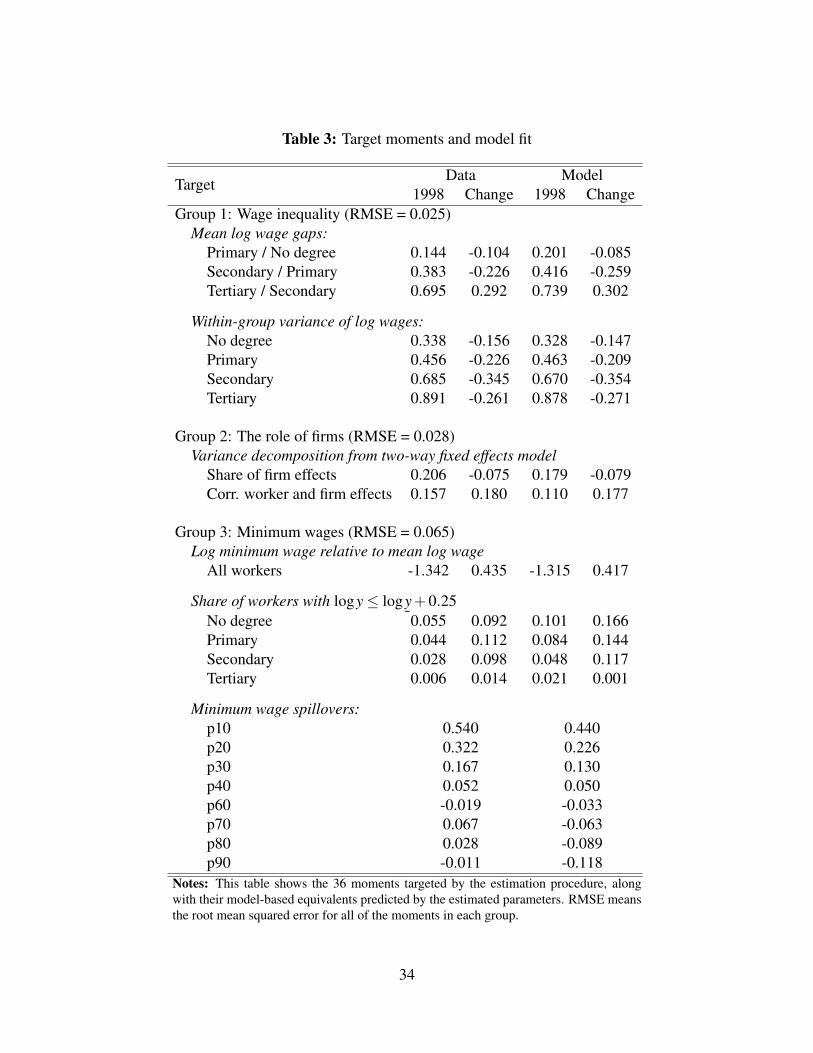
Table 3: Target moments and model fit

TargetData Model

1998 Change 1998 ChangeGroup 1: Wage inequality (RMSE = 0.025)

Mean log wage gaps:Primary / No degree 0.144 -0.104 0.201 -0.085Secondary / Primary 0.383 -0.226 0.416 -0.259Tertiary / Secondary 0.695 0.292 0.739 0.302

Within-group variance of log wages:No degree 0.338 -0.156 0.328 -0.147Primary 0.456 -0.226 0.463 -0.209Secondary 0.685 -0.345 0.670 -0.354Tertiary 0.891 -0.261 0.878 -0.271

Group 2: The role of firms (RMSE = 0.028)Variance decomposition from two-way fixed effects model

Share of firm effects 0.206 -0.075 0.179 -0.079Corr. worker and firm effects 0.157 0.180 0.110 0.177

Group 3: Minimum wages (RMSE = 0.065)Log minimum wage relative to mean log wage

All workers -1.342 0.435 -1.315 0.417

Share of workers with logy≤ log¯y+0.25

No degree 0.055 0.092 0.101 0.166Primary 0.044 0.112 0.084 0.144Secondary 0.028 0.098 0.048 0.117Tertiary 0.006 0.014 0.021 0.001

Minimum wage spillovers:p10 0.540 0.440p20 0.322 0.226p30 0.167 0.130p40 0.052 0.050p60 -0.019 -0.033p70 0.067 -0.063p80 0.028 -0.089p90 -0.011 -0.118

Notes: This table shows the 36 moments targeted by the estimation procedure, alongwith their model-based equivalents predicted by the estimated parameters. RMSE meansthe root mean squared error for all of the moments in each group.

34

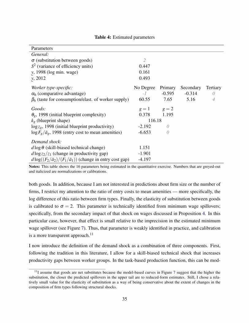
Table 4: Estimated parameters

ParametersGeneral:σ (substitution between goods) 2S2 (variance of efficiency units) 0.447

¯y, 1998 (log min. wage) 0.161

¯y, 2012 0.493

Worker type-specific: No Degree Primary Secondary Tertiaryαh (comparative advantage) -1 -0.595 -0.314 0βh (taste for consumption/elast. of worker supply) 60.55 7.65 5.16 4

Goods: g = 1 g = 2θg, 1998 (initial blueprint complexity) 0.378 1.195kg (blueprint shape) 116.18logzg, 1998 (initial blueprint productivity) -2.192 0logFg/ag, 1998 (entry cost to mean amenities) -6.653 0

Demand shock:d logθ (skill-biased technical change) 1.151d logz2/z1 (change in productivity gap) -1.901d log((F2/a2)/(F1/a1)) (change in entry cost gap) -4.197

Notes: This table shows the 16 parameters being estimated in the quantitative exercise. Numbers that are greyed-outand italicized are normalizations or calibrations.

both goods. In addition, because I am not interested in predictions about firm size or the number offirms, I restrict my attention to the ratio of entry costs to mean amenities — more specifically, thelog difference of this ratio between firm types. Finally, the elasticity of substitution between goodsis calibrated to σ = 2. This parameter is technically identified from minimum wage spillovers;specifically, from the secondary impact of that shock on wages discussed in Proposition 4. In thisparticular case, however, that effect is small relative to the imprecision in the estimated minimumwage spillover (see Figure 7). Thus, that parameter is weakly identified in practice, and calibrationis a more transparent approach.11

I now introduce the definition of the demand shock as a combination of three components. First,following the tradition in this literature, I allow for a skill-biased technical shock that increasesproductivity gaps between worker groups. In the task-based production function, this can be mod-

11I assume that goods are net substitutes because the model-based curves in Figure 7 suggest that the higher thesubstitution, the closer the predicted spillovers in the upper tail are to reduced-form estimates. Still, I chose a rela-tively small value for the elasticity of substitution as a way of being conservative about the extent of changes in thecomposition of firm types following structural shocks.

35

eled as a proportional increase in task complexities d logθ , as shown in Proposition 3. The secondcomponent is a possible change in the relative productivity of firm types, d logz2/z1. This compo-nent affects the overall employment share of each firm type. The third component is a change inthe relative ratio of entry costs to amenities, d log((F2/a2)/(F2/a2)). That relative ratio is a keydeterminant of cross-firm wage dispersion for similar workers.

The last parameters in the model are minimum wages relative to the price of entry inputs (thenumeraire in the model). Minimum wages are added as a free parameter procedure because pricesfor goods, entrepreneurial talent, and labor are unobserved, making a direct calibration of thatparameter impossible.

4.2.2 Estimation procedure

The model is estimated by minimizing the least squares distance between the observed momentsin Table 3 and the model equivalent of these moments. Each of the three groups of moments havethe same importance in estimation. To evaluate the loss function, I need a function that maps thevectors of parameters to the vectors of moments predicted by two equilibria of the model, onecorresponding to 1998 and another corresponding to 2012. To find these equilibria given a set ofcandidate models, I use a slightly modified set of equilibrium conditions: instead of imposing thatthe number of job applicants equals the total number of workers of each type (which is unobservedin the data), I impose instead that the number of employed workers in the model equals observedemployment.12

The first group of moments in Table 3, along with the measures of how binding the minimum wageis in the third group, are calculated from the model-implied wage distributions for each worker type.Minimum wage spillovers are calculated as follows. First, I take each of the estimated equilibriaand calculate a counterfactual where the log minimum wage increases by 10−6 relative to the entryinput. Next, consistent with the reduced form specification (Equation 12), I calculate the changesin each quantile p over the change in the minimum wage, both of which are relative to the medianwage: ∆[y(p)− y(50)]/∆[

¯y− y(50)]. Finally, I use the average of spillovers across both periods

(1998 and 2012) as the model-based analogues of the reduced form estimates.

I simulate the model-predicted variance decomposition from an AKM regression using a large firms

12This approach is computationally more efficient than adding parameters for total labor supply Nh and additionalmoments for observed employment. They are not completely equivalent because the latter can account for samplingerror in observed employment shares by worker group. Given the large sample size, this difference is unlikely to berelevant in practice.

36

assumption. When firms are large, the internal distributions of worker types and wages in a firm oftype g are approximately the same as the model-predicted distributions for that type. Thus, firmsof the same type in the model are statistically identical except for size. I also need a stylized modelof employment dynamics, because the model described in the previous section is static. Definea worker type i as a tuple (hi,εi). First, I assume that there is mobility between firm types forall worker types i that are not rejected by either firm. Second, I assume that εit is a combinationof a portable human capital component (the worker fixed effect) plus a transient effect, with therelevance of the transient effect calibrated so that the share of the variance of log wages attributableto the residual is of similar size to that in the data.13

Given these assumptions, the variance decomposition is calculated from a simulation of the modelwhere there are only two large firms in the economy, one for each firm type. First, I discretize thedistribution of efficiency units ε , so that there is a discrete number of worker types (hi,εi). Then, Isimulate a data set where each observation is a combination of worker type i and firm type g. Thisdata set contains indicators for firm and worker type, worker earnings, and weights constructedfrom the model-predicted mass of workers of each type i employed by firms of each type g. Next,I estimate firm and worker effects via a weighted ordinary least squares regression of log earningson firm and worker type dummies.14 Finally, I calculate the variance decomposition componentsusing those estimated fixed effects.

The parametric space is the real line for parameters defined in logs and the positive real line formost others. The exceptions are comparative advantages αh ∈ (0,1) and βh ∈ (1,100). Standarderrors will be provided in a future version of this paper.

4.2.3 Estimates, goodness of fit, and discussion

Table 4 shows the estimated parameters and Table 3 illustrates the moments predicted by the esti-mated model. Overall, the model fits the data well, particularly for the first two groups of moments(levels and trends in wage inequality and components of the variance decomposition based on thetwo-way fixed effects regressions). That the model fits within-group variances well is particularlyinteresting given the restriction that the variance of labor efficiency units is the same for all groupsand both periods.

13Formally, I set εit = εFi + εT

it , with the transitory component εTit orthogonal to the fixed component εF

i . Thevariances of each of these components is calibrated so that (i) the variance of εit is the parameter S2; and (ii) theestimated share of the residuals in the model-based variance decomposition is 0.9.

14OLS estimates are consistent in this regression because the number of firm fixed effects being estimated does notgrow with the sample size.

37

Figure 6: Distribution of log wages, data and model

(a) Data

0

.02

.04

.06

0 1 2 3 4

Group 1

0

.02

.04

.06

0 1 2 3 4

Group 2

0

.02

.04

.06

0 1 2 3 4

Group 3

0

.02

.04

.06

0 1 2 3 4

Group 4

(b) Simulation from estimated model

Notes: This figure shows histograms of log wages using 0.05-sized bins, separatelyby educational group (No degree, Primary, Secondary, and Tertiary) and time (1998in blue, 2012 in red). Panel (a) shows data from RAIS, Rio Grande do Sul, Brazil,hours-weighted. Panel (b) shows histograms predicted by the estimated model.

38

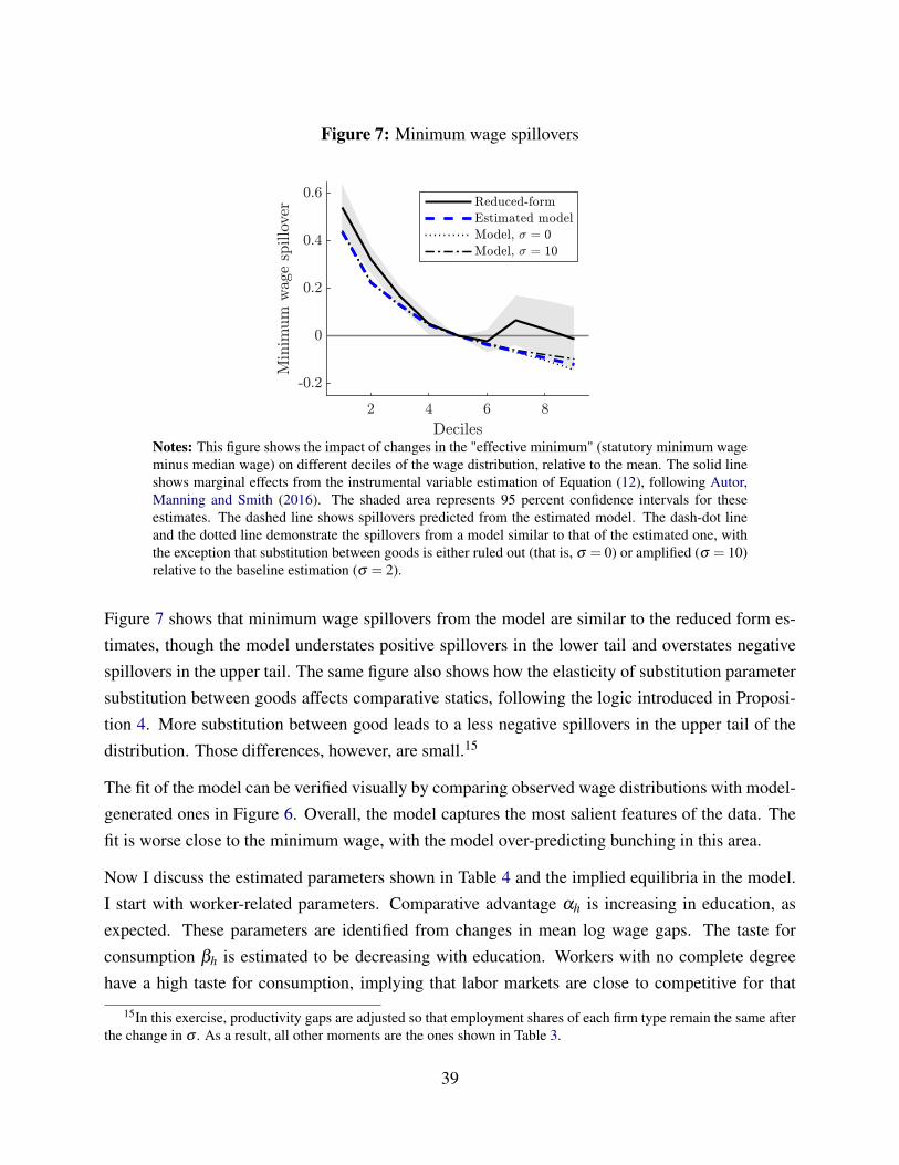
Figure 7: Minimum wage spillovers

Notes: This figure shows the impact of changes in the "effective minimum" (statutory minimum wageminus median wage) on different deciles of the wage distribution, relative to the mean. The solid lineshows marginal effects from the instrumental variable estimation of Equation (12), following Autor,Manning and Smith (2016). The shaded area represents 95 percent confidence intervals for theseestimates. The dashed line shows spillovers predicted from the estimated model. The dash-dot lineand the dotted line demonstrate the spillovers from a model similar to that of the estimated one, withthe exception that substitution between goods is either ruled out (that is, σ = 0) or amplified (σ = 10)relative to the baseline estimation (σ = 2).

Figure 7 shows that minimum wage spillovers from the model are similar to the reduced form es-timates, though the model understates positive spillovers in the lower tail and overstates negativespillovers in the upper tail. The same figure also shows how the elasticity of substitution parametersubstitution between goods affects comparative statics, following the logic introduced in Proposi-tion 4. More substitution between good leads to a less negative spillovers in the upper tail of thedistribution. Those differences, however, are small.15

The fit of the model can be verified visually by comparing observed wage distributions with model-generated ones in Figure 6. Overall, the model captures the most salient features of the data. Thefit is worse close to the minimum wage, with the model over-predicting bunching in this area.

Now I discuss the estimated parameters shown in Table 4 and the implied equilibria in the model.I start with worker-related parameters. Comparative advantage αh is increasing in education, asexpected. These parameters are identified from changes in mean log wage gaps. The taste forconsumption βh is estimated to be decreasing with education. Workers with no complete degreehave a high taste for consumption, implying that labor markets are close to competitive for that

15In this exercise, productivity gaps are adjusted so that employment shares of each firm type remain the same afterthe change in σ . As a result, all other moments are the ones shown in Table 3.

39

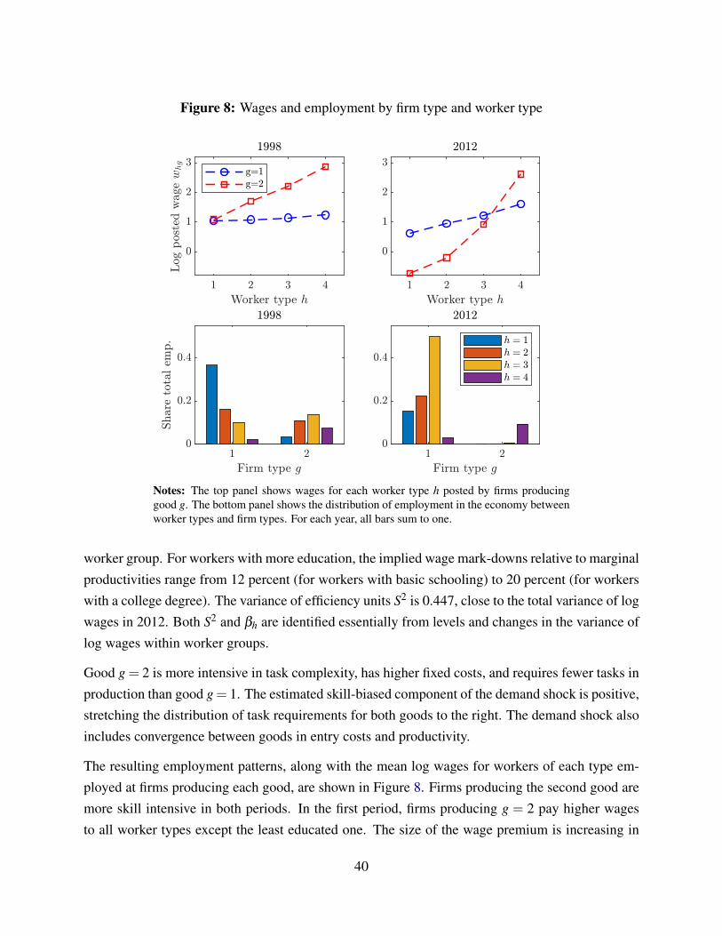
Figure 8: Wages and employment by firm type and worker type

Notes: The top panel shows wages for each worker type h posted by firms producinggood g. The bottom panel shows the distribution of employment in the economy betweenworker types and firm types. For each year, all bars sum to one.

worker group. For workers with more education, the implied wage mark-downs relative to marginalproductivities range from 12 percent (for workers with basic schooling) to 20 percent (for workerswith a college degree). The variance of efficiency units S2 is 0.447, close to the total variance of logwages in 2012. Both S2 and βh are identified essentially from levels and changes in the variance oflog wages within worker groups.

Good g = 2 is more intensive in task complexity, has higher fixed costs, and requires fewer tasks inproduction than good g= 1. The estimated skill-biased component of the demand shock is positive,stretching the distribution of task requirements for both goods to the right. The demand shock alsoincludes convergence between goods in entry costs and productivity.

The resulting employment patterns, along with the mean log wages for workers of each type em-ployed at firms producing each good, are shown in Figure 8. Firms producing the second good aremore skill intensive in both periods. In the first period, firms producing g = 2 pay higher wagesto all worker types except the least educated one. The size of the wage premium is increasing in

40

worker type. These differences stem from a combination of increased demand for skilled workersalong with a higher ratio of entry costs to amenities in the second firm type relative to the first, asdescribed in Proposition 2. These differences explain both the substantial share of firm effects inthe variance of log wages and why the estimated firm effects from the log-additive model correlatewith worker effects.

In the second period, firms producing g = 2 still pay more to skilled workers. However, theypost lower wages for less skilled workers, reflect extremely low labor demand for them. Thecombination of these effects explains why firm fixed effects become less relevant as a share of thetotal variance of log wages, while at the same time the correlation between worker and firm fixedeffects increases.

I interpret the demand shock as follows. In the first period, the first good, g = 1 represents a "back-ward" technology intensive in low-complexity tasks. The second good, g= 2 represents a "modern"technology that has higher returns to education. The demand shock replaces the "backward" tech-nology to another that uses more complex tasks and is closer to the modern one in entry costs andphysical productivity. At the same time, the "modern" technology is also affected by skill-biasedtechnical change, becoming even more specialized in high-complexity tasks. Following a concur-rent increase in the supply of education, firms producing the modern good find it profitable to fullyspecialize in college-educated workers.

4.3 Disentangling the role of supply, demand, and minimum wages

In this final step, I use the model to generate counterfactuals that isolate the role of supply, demand,and minimum wage shocks. The first counterfactual scenario has all parameters from the estimatedmodel in 1998, except for labor supply —- which changes to the 2012 levels – and minimum wages,which adjust relative to the numeraire of the model so that it remains constant relative to mean logwages.16 Next, I move from this scenario to another where the demand shocks occurred, and theminimum wage is still kept constant relative to mean log wages. Finally, the last step measures

16It is easy to observe the number of employed workers in each educational group, but it is not obvious how tomeasure total labor supply Nh in the model due to involuntary non-employment. I use a structural approach to dealwith this issue. The estimation procedure looks for one equilibrium in the model for each period such that the modelpredictions (including share of employment by education) match the data. After the equilibrium and its correspondingset of parameters is identified, the parametric assumption of the distribution of efficiency units allows the researcher toextrapolate the number of unemployed workers, thus obtaining the total labor supply Nh. Thus, the change imposedin the first counterfactual is moving from the estimated Nh for the 1998 equilibrium to the one coming from the 2012equilibrium.

41

Table 5: Model-based decomposition: supply, demand, and minimum wages.

Moment All changes Supply Demand Minimum wageVariance of log wages -0.201 0.004 -0.079 -0.125

Mean log wage gaps:Primary / No degree -0.085 -0.081 0.102 -0.106Secondary / Primary -0.259 -0.088 -0.100 -0.070Tertiary / Secondary 0.302 -0.010 0.424 -0.112

Within-group variance of log wages:No degree -0.147 -0.007 -0.032 -0.108Primary -0.209 -0.034 -0.064 -0.111Secondary -0.354 -0.038 -0.225 -0.091Tertiary -0.271 0.073 -0.327 -0.017

Variance decomposition from two-way fixed effects modelShare of firm effects -0.079 0.081 -0.193 0.033Corr. worker and firm effects 0.177 -0.080 0.281 -0.024

Notes: The meaning of each column is as follows: All changes denotes changes predicted by theestimated model, comparing the 1998 equilibrium to the 2012 equilibrium. Supply shows differencesbetween the 1998 equilibrium and a counterfactual equilibrium using 1998 parameters, except for thenumber of workers of each type (changed to the 2012 value) and minimum wages (adjusted so that theminimum wage to mean log wage remains constant). Demand shows the differences between the firstcounterfactual and a second counterfactual where the demand shock is imposed, while still holdingminimum wages stable relative to mean log wages. Minimum wage shows differences between thesecond counterfactual and the 2012 equilibrium.

the difference from this second counterfactual to the estimated model in the second period, whichincludes changes in all dimensions.

Before showing the results of this model-based decomposition, it is worth noting that this exerciserequires a strong assumption: each of these components is entirely exogenous, such that movingeither one in isolation is a meaningful counterfactual. One example of a deviation would be anendogenous technical response to increased availability of qualified labor. Another example islabor supply responses to changes in wages following demand and minimum wage shocks. Thelabor supply example is particularly relevant for two reasons. First, in contrast to other model-basedexercises, I do not restrict the sample to male workers, a group that usually has a low elasticity oflabor supply. Second, the informal sector provides an "outside option" for workers in the formalsector, and the gap in attractiveness between formal and informal jobs might be a complicatedfunction of the labor supply, technical change, and minimum wages (Haanwinckel and Soares,2016). A model-based account of the informal sector is possible, but it is beyond the scope of this

42

paper.

Even with these limitations, this exercise can still shed light on the causes of decreased inequalityin Brazil, because it incorporates equilibrium effects while studying a wide range of shocks. Thereare some model-based decompositions of wage inequality in Brazil, but they focus on smaller setsof shocks and causal mechanisms relative to this paper. Engbom and Moser (2018) develop a modelof between-firm wage dispersion and focus on the role of the minimum wage, but do not accountfor equilibrium effects of changes in educational achievement and technical change. Mak and Siow(2018) build a model of within-firm complementarities between workers and use it to study therole of labor supply. That paper does not feature between-firm wage dispersion and minimumwages. Finally, (Ferreira, Firpo and Messina, 2017) performs a decomposition exercise that fea-tures a broad array of explanatory factors and includes both the formal and informal sectors. Thatexercise, however, does not account for equilibrium effects of changes in labor supply, demand,and institutions; while helpful as a descriptive tool and for ruling out some possible explanations,it does not offer measurements of the causal effect of each shock.

With these caveats in mind, I discuss the results of the model-based decomposition. The supplyshock reduces mean log wage gaps among workers with less than tertiary education, but have noeffect on the returns to college relative to high school. These effects are consistent with a straight-forward supply-demand intuition, since the supply of high school and college educated workersincreases substantially. The effects on within-group variances of log wages is small. Finally,the overall effect on the total variance of log wages is null; even though there are reductions inbetween-group log wage gaps, there is also an endowment effect that increases the overall dis-persion of wages in the economy. This result is similar to the conclusions in Ferreira, Firpo andMessina (2017). The supply shock also causes a moderate increase in the share of the variance oflog wages explained by firm effects, along with a moderate decline in the correlation of worker andfirm fixed effects.

As described in the previous subsection, the estimated demand shock is a combination of skill-biased technical change (modeled as a drift towards more complex tasks) and convergence betweenfirm types in entry costs and productivity. With a representative firm, increased task complexityshould widen all between-group wage gaps. Following this logic, there is a large increase in wagesfor college-educated workers. However, high school workers lose relative to those with only pri-mary education. The reason for this "wage polarization" effect is the loss of firm-level wage premiafor high-school workers. Without the minimum shock, most workers in this group are employed by"modern" firms where their skills are valuable. As described in the previous section, the demand

43

shock induces "modern" firms to fully specialize in college-educated workers. The high schoolworkers are then reallocated to "backward" firms, where their comparative advantage relative toless-educated workers is smaller.

The demand shock also causes reductions in cross-firm wage dispersion, which reflect in an overalldecline in wage inequality. There are two separate channels leading to these reductions. First,because the modern firms specialize in college-educated workers following the increase in taskcomplexity, there is effectively no cross-firm wage dispersion for workers up to high school in thesecond period. That explains decreased within-group inequality for these workers following thedemand shock. In addition, the reduction in the entry cost gap between goods reduced the sizeof the cross-firm wage premia for college educated workers, with corresponding consequences forthe variance of log wages within that group. The combined effect of these changes is a sizablereduction in overall inequality, accounting for almost 40 percent of the total decline in the varianceof log wages.

The demand shock also makes the labor market more assortative, as measured by the correlationbetween worker and firm fixed effects in the AKM regressions. This result follows from full spe-cialization in college-educated workers in the modern firms, along with the fact that the wagepremia for these workers remain positive (though smaller in magnitude).

The minimum wage is the most important factor explaining declining wage inequality in this con-text. It has sizable effects in both between-group and within-group inequality. I also find thatminimum wages have small impacts on the share of the variance of log wages explained by firmeffects and in the correlation between worker and firm effects. These results are similar to those inEngbom and Moser (2018).

5 Conclusion

This paper demonstrated that a task-based model of production is a useful tool for modeling firmheterogeneity in imperfectly competitive labor markets. The theory reveals two kinds of novel in-teractions between the supply-demand-institutions framework commonly employed to study wageinequality and the applied microeconomic literature examining imperfect competition in labor mar-kets using matched employer-employee data. First, shocks to labor supply, labor demand, and min-imum wages affect between-firm wage dispersion and labor market sorting. Second, adding firmheterogeneity and imperfect competition to the traditional approach leads to aggregation issues that

44

might change how those shocks affect the wage distribution in a qualitative sense.

The application of the model using Brazilian data showed that the channels introduced in the theoryare relevant for explaining the evolution of inequality and labor market sorting. It also showedthat demand-side shocks, including skill-biased technical change, play essential roles in the labormarket transformations in Brazil, despite the observed declines in wage inequality.

I conclude this section by discussing two directions for further research. First, a version of themodel with capital provides a tool for modeling different forms of technical changes, as well ascapital-skill complementarity. Acemoglu and Autor (2011) employ a task-based structure to modelroutine-biased technical change resulting from price reductions for types of capital particularly ef-fective at tasks executed by mid-skill workers. The same idea can be introduced in this framework.A simple way to do so is to include different vintages of capital, all of which perfectly substitute forlabor at individual tasks but with varying schedules of productivity. This is simple from a model-ing perspective because capital vintages behave as worker types do, thus requiring no modificationof the model. Each vintage is then a substitute for some worker types and a complement to oth-ers. A different approach is to assume capital and labor are imperfect substitutes in the productionof tasks, and that this elasticity of substitution decreases in task complexity. This provides a mi-crofoundation for capital-skill complementarity, a pattern that has been documented in the labordemand literature (Hamermesh, 1996) and that is potentially relevant for explaining trends in wageinequality (Krusell et al., 1999).

The model can also be used to quantify the impact of trade shocks on wages. Economists haveincreasingly used models with heterogeneous firms when studying the inequality effects of trade.Some papers (Sampson, 2014; Burstein, Morales and Vogel, 2016; Burstein and Vogel, 2017) show,using competitive models, that trade liberalization can affect the returns to skill because it favorsfirms that are more skill-intensive. Others (Helpman, Itskhoki and Redding, 2010; Davis and Harri-gan, 2011; Helpman et al., 2017) highlight that trade opening can also increase between-firm wagedispersion for similar workers when labor markets are not competitive. The model developed inthis paper can combine both perspectives, while also accounting for the ex-ante worker heterogene-ity in productivity, firm-to-worker sorting, and other shocks to wage inequality coming from thetraditional supply-demand-institutions framework.

45

References

Abowd, John M, Francis Kramarz, and David N Margolis. 1999. “High Wage Workers andHigh Wage Firms.” Econometrica, 67(2): 251–333.

Abowd, John M., Francis Kramarz, Sébastien Pérez-Duarte, and Ian M. Schmutte. 2018.“Sorting Between and Within Industries: A Testable Model of Assortative Matching.” Annals of

Economics and Statistics, , (129): 1–32.

Acemoglu, Daron. 1999. “Changes in Unemployment and Wage Inequality: An Alternative The-ory and Some Evidence.” The American Economic Review, 89(5): 1259–1278.

Acemoglu, Daron. 2001. “Good Jobs versus Bad Jobs.” Journal of Labor Economics, 19(1): 1–21.

Acemoglu, Daron, and David Autor. 2011. “Skills, Tasks and Technologies: Implications forEmployment and Earnings.” In Handbook of Labor Economics. Vol. 4, Part B, , ed. David Cardand Orley Ashenfelter, Chapter 12, 1043–1171. Elsevier.

Acemoglu, Daron, and Pascual Restrepo. 2018. “Artificial Intelligence, Automation and Work.”National Bureau of Economic Research Working Paper 24196.

Alvarez, Jorge, Felipe Benguria, Niklas Engbom, and Christian Moser. 2018. “Firms andthe Decline in Earnings Inequality in Brazil.” American Economic Journal: Macroeconomics,10(1): 149–89.

Andrews, M. J., L. Gill, T. Schank, and R. Upward. 2008. “High wage workers and low wagefirms: negative assortative matching or limited mobility bias?” Journal of the Royal Statistical

Society: Series A (Statistics in Society), 171(3): 673–697.

Antràs, Pol, Luis Garicano, and Esteban Rossi-Hansberg. 2006. “Offshoring in a KnowledgeEconomy.” The Quarterly Journal of Economics, 121(1): 31–77.

Ashenfelter, Orley C., Henry Farber, and Michael R Ransom. 2010. “Labor Market Monop-sony.” Journal of Labor Economics, 28(2): 203–210.

Autor, David H. 2014. “Skills, education, and the rise of earnings inequality among the other 99percent.” Science, 344(6186): 843–851.

Autor, David H., Alan Manning, and Christopher L. Smith. 2016. “The Contribution of theMinimum Wage to US Wage Inequality over Three Decades: A Reassessment.” American Eco-

nomic Journal: Applied Economics, 8(1): 58–99.

46

Autor, David H, Frank Levy, and Richard J Murnane. 2003. “The Skill Content of Re-cent Technological Change: An Empirical Exploration.” The Quarterly Journal of Economics,118(4): 1279–1333.

Autor, David H, Lawrence F Katz, and Melissa S Kearney. 2008. “Trends in U.S. Wage Inequal-ity: Revising the Revisionists.” The Review of Economics and Statistics, 90(2): 300–323.

Bound, John, and George Johnson. 1992. “Changes in the Structure of Wages in the 1980’s: AnEvaluation of Alternative Explanations.” The American Economic Review, 82(3): 371–392.

Burstein, Ariel, and Jonathan Vogel. 2017. “International Trade, Technology, and the Skill Pre-mium.” Journal of Political Economy, 125(5): 1356–1412.

Burstein, Ariel, Eduardo Morales, and Jonathan Vogel. 2016. “Changes in between-group in-equality: computers, occupations, and international trade.”

Caliendo, Lorenzo, and Esteban Rossi-Hansberg. 2012. “The Impact of Trade on Organizationand Productivity.” The Quarterly Journal of Economics, 127(3): 1393–1467.

Card, David, Ana Rute Cardoso, Joerg Heining, and Patrick Kline. 2018. “Firms and LaborMarket Inequality: Evidence and Some Theory.” Journal of Labor Economics, 36(S1): S13–S70.

Card, David, and John E DiNardo. 2002. “Skill-Biased Technological Change and Rising WageInequality: Some Problems and Puzzles.” Journal of Labor Economics, 20(4): 733–783.

Card, David, and Thomas Lemieux. 2001. “Can Falling Supply Explain the Rising Return toCollege for Younger Men? A Cohort-Based Analysis.” The Quarterly Journal of Economics,116(2): 705–746.

Card, David, Jörg Heining, and Patrick Kline. 2013. “Workplace Heterogeneity and the Rise ofWest German Wage Inequality.” The Quarterly Journal of Economics, 128(3): 967.

Cengiz, Doruk, Arindrajit Dube, Attila Lindner, and Ben Zipperer. 2018. “The Effect of Mini-mum Wages on Low-Wage Jobs: Evidence from the United States Using a Bunching Estimator.”Centre for Economic Performance, LSE CEP Discussion Papers dp1531.

Chade, Hector, Jan Eeckhout, and Lones Smith. 2017. “Sorting through Search and MatchingModels in Economics.” Journal of Economic Literature, 55(2): 493–544.

Coase, R H. 1937. “The Nature of the Firm.” Economica, 4(16): 386–405.

47

Costinot, Arnaud, and Jonathan Vogel. 2010. “Matching and Inequality in the World Economy.”Journal of Political Economy, 118(4): 747–786.

Cragg, John G., and Stephen G. Donald. 1993. “Testing Identifiability and Specification in In-strumental Variable Models.” Econometric Theory, 9(2): 222–240.

Davis, Donald R., and James Harrigan. 2011. “Good jobs, bad jobs, and trade liberalization.”Journal of International Economics, 84(1): 26 – 36.

de Melo, Rafael Lopes. 2018. “Firm Wage Differentials and Labor Market Sorting: ReconcilingTheory and Evidence.” Journal of Political Economy, 126(1): 313–346.

De Negri, João Alberto, Paulo Furtado de Castro, Natalia Ribeiro de Souza, and Jorge SabaArbache. 2001. “Mercado Formal de Trabalho: Comparação entre os Microdados da RAIS e daPNAD.” IPEA Texto para Discussão 840.

DiNardo, John, Nicole M Fortin, and Thomas Lemieux. 1996. “Labor Market Institutionsand the Distribution of Wages, 1973-1992: A Semiparametric Approach.” Econometrica,64(5): 1001–1044.

Eeckhout, Jan, and Philipp Kircher. 2011. “Identifying Sorting—In Theory.” The Review of

Economic Studies, 78(3): 872–906.

Eeckhout, Jan, and Philipp Kircher. 2018. “Assortative Matching With Large Firms.” Economet-

rica, 86(1): 85–132.

Engbom, Niklas, and Christian Moser. 2018. “Earnings Inequality and the Minimum Wage:Evidence from Brazil.” Federal Reserve Bank of Minneapolis, Opportunity and Inclusive GrowthInstitute Working Papers 7.

Ferreira, Francisco H. G., Sergio P. Firpo, and Julián Messina. 2017. “Ageing Poorly?: Ac-counting for the Decline in Earnings Inequality in Brazil, 1995-2012.” Inter-American Develop-ment Bank IDB Publications (Working Papers) 8220.

Garicano, Luis. 2000. “Hierarchies and the Organization of Knowledge in Production.” Journal of

Political Economy, 108(5): 874–904.

Garicano, Luis, and Esteban Rossi-Hansberg. 2006. “Organization and Inequality in a Knowl-edge Economy.” The Quarterly Journal of Economics, 121(4): 1383–1435.

Gautier, Pieter A, and Coen N Teulings. 2015. “Sorting and the Output Loss due to SearchFrictions.” Journal of the European Economic Association, 13(6): 1136–1166.

48

Gautier, Pieter A, Coen N Teulings, and Aico van Vuuren. 2010. “On-the-Job Search, Mismatchand Efficiency.” The Review of Economic Studies, 77(1): 245–272.

Grossman, Gene M, Elhanan Helpman, and Philipp Kircher. 2017. “Matching, Sorting, and theDistributional Effects of International Trade.” Journal of Political Economy, 125(1): 224–264.

Haanwinckel, Daniel, and Rodrigo R. Soares. 2016. “Workforce Composition, Productivity, andLabor Regulations in a Compensating Differentials Theory of Informality.” Institute for the Studyof Labor (IZA) IZA Discussion Papers 9951.

Hamermesh, Daniel S. 1996. Labor demand. princeton University press.

Harasztosi, Péter, and Attila Lindner. 2018. “Who Pays for the Minimum Wage?” Unpublishedmanuscript.

Helpman, Elhanan, Oleg Itskhoki, and Stephen Redding. 2010. “Inequality and Unemploymentin a Global Economy.” Econometrica, 78(4): 1239–1283.

Helpman, Elhanan, Oleg Itskhoki, Marc-Andreas Muendler, and Stephen J Redding. 2017.“Trade and Inequality: From Theory to Estimation.” The Review of Economic Studies, 84(1): 357.

Hornstein, Andreas, Per Krusell, and Giovanni L. Violante. 2011. “Frictional Wage Dispersionin Search Models: A Quantitative Assessment.” The American Economic Review, 101(7): 2873–2898.

Katz, Lawrence F, and Kevin M Murphy. 1992. “Changes in Relative Wages, 1963-1987: Supplyand Demand Factors.” The Quarterly Journal of Economics, 107(1): 35–78.

Kline, P., R. Saggio, and M. Sølvsten. 2018. “Leave-out estimation of variance components.”ArXiv e-prints.

Kremer, Michael, and Eric Maskin. 1996. “Wage Inequality and Segregation by Skill.” NationalBureau of Economic Research Working Paper 5718.

Krugman, Paul. 1985. “A ‘Technology Gap’ Model of International Trade.” Structural Adjust-

ment in Developed Open Economies, , ed. Karl Jungenfelt and Douglas Hague, 35–61. Lon-don:Palgrave Macmillan UK.

Krusell, Per, Lee E Ohanian, José-Víctor Ríos-Rull, and Giovanni L Violante. 1999.“Capital-skill Complementarity and Inequality: A Macroeconomic Analysis.” Econometrica,68(5): 1029–1053.

49

Lee, David S. 1999. “Wage Inequality in the United States during the 1980s: Rising Dispersion orFalling Minimum Wage?” The Quarterly Journal of Economics, 114(3): 977–1023.

Lentz, Rasmus, and Dale T Mortensen. 2010. “Labor market models of worker and firm hetero-geneity.” Annu. Rev. Econ., 2(1): 577–602.

Lindenlaub, Ilse. 2017. “Sorting Multidimensional Types: Theory and Application.” The Review

of Economic Studies, 84(2): 718–789.

Lindenlaub, Ilse, and Fabien Postel-Vinay. 2017. “Multidimensional Sorting Under RandomSearch.” Unpublished manuscript.

Lise, Jeremy, Costas Meghir, and Jean-Marc Robin. 2016. “Matching, sorting and wages.” Re-

view of Economic Dynamics, 19: 63 – 87. Special Issue in Honor of Dale Mortensen.

Mak, Eric, and Aloysius Siow. 2018. “Occupational Choice, Matching and Earnings Inequality.”Unpublished manuscript.

Manning, Alan. 2011. “Imperfect Competition in the Labor Market.” In Handbook of Labor Eco-

nomics. Vol. 4, Part B, , ed. David Card and Orley Ashenfelter, Chapter 11, 973–1041. Elsevier.

Sampson, Thomas. 2014. “Selection into Trade and Wage Inequality.” American Economic Jour-

nal: Microeconomics, 6(3): 157–202.

Shimer, Robert. 2005. “The Assignment of Workers to Jobs in an Economy with CoordinationFrictions.” Journal of Political Economy, 113(5): 996–1025.

Song, Jae, David J. Price, Fatih Guvenen, Nicholas Bloom, and Till von Wachter. 2018. “Firm-ing Up Inequality.” Forthcoming, The Quarterly Journal of Economics.

Teulings, Coen N. 1995. “The Wage Distribution in a Model of the Assignment of Skills to Jobs.”Journal of Political Economy, 103(2): 280–315.

Teulings, Coen N. 2000. “Aggregation Bias in Elasticities of Substitution and the Minimum WageParadox.” International Economic Review, 41(2): 359–398.

Teulings, Coen N. 2003. “The Contribution of Minimum Wages to Increasing Wage Inequality.”The Economic Journal, 113(490): 801–833.

Teulings, Coen N. 2005. “Comparative Advantage, Relative Wages, and the Accumulation of Hu-man Capital.” Journal of Political Economy, 113(2): 425–461.

50

A Proofs

Section 2: Task-based production function

Proof of Lemma 1: Allocation is assortative and labor constraints bind

I proceed by proving two lemmas that, together, imply the desired result. I use the term candidate

solution to refer to tuples of output and schedules{

q,{mh}Hh=1}

that satisfy all constraints in theassignment problem.Lemma 3. If there exists a candidate solution

{q,{mh(·)}H

h=1}

such that one can find two tasks

x1 < x2 and two worker types h1 < h2 with mh1(x2) > 0 and mh2(x1) > 0, then there exists an

alternative candidate solution{

q′,{m′h(·)}Hh=1}

that achieves the same output (q = q′) but has a

slack of labor of type h1 (lh1 >∫

∞

0 m′h1(x)dx).

Proof. Let ∆ = x2− x1 and pick τ ∈ (0,min{mh1(x2),mh2(x1)eh2(x1 +∆)/eh1(x1 +∆)}). Becausemh(·) is right continuous and the efficiency functions eh(·) are strictly positive and continuous, Ican find δ > 0 such that mh1(x)> τ ∀x ∈ [x2,x2+δ ) and mh2(x1)eh2(x1+∆)/eh1(x1+∆)> τ ∀x ∈[x1,x1 +δ ).

Now construct{

q′,{m′h(·)}Hh=1}

identical to{

q,{mh(·)}Hh=1}

, except for:

m′h1(x) = mh1(x)− τ, x ∈ [x2,x2 +δ )

m′h2(x) = mh2(x)+ τ

eh1(x)eh2(x)

, x ∈ [x2,x2 +δ )

m′h2(x) = mh2(x)− τ

eh1(x+∆)

eh2(x+∆), x ∈ [x1,x1 +δ )

m′h1(x) = mh1(x)+ τ

eh1(x+∆)

eh2(x+∆)

eh2(x)eh1(x)

, x ∈ [x1,x1 +δ )

I need to prove that{

q′,{m′h(·)}Hh=1}

satisfies all constraints in the assignment problem and has aslack of labor h1, and that m′h(·) ∈ RC. Starting with the latter, note that m′h(·) is always identical tomh(·) except in intervals of the form [a,b). In those intervals, m′h(·) is a continuous transformationof mh(·). So, because mh(·) is right continuous, so is m′h(·). In addition, m′h(x) > 0 ∀x ∈ R>0 bythe condition imposed when defining δ . So m′h(·) ∈ RC.

Next, the blueprint constraints are satisfied under the new candidate solution because second and

51

fourth rows increase task production of particular complexities in a way that exactly offsets de-creased production due to the first and third rows, respectively. Total labor use of type h2 is identicalunder both allocations, because the additional assignment in the second row is offset by reduced as-signment in the third row. Finally, decreased use of labor type h1 follows from log-supermodularityof the efficiency functions, which guarantees that the term multiplying τ in the fourth row is strictlyless than one. So labor added in that row is strictly less than labor saved in the first row.

Lemma 4. Any candidate solution with slack of labor is not optimal.

Proof. Consider two cases:

If there is slack of labor of the highest type, h = H: By the feasibility condition in the definitionof blueprints, uH =

∫∞

0 b(x)/eH(x)dx is finite. Denote the slack of labor of type H in the originalcandidate solution by SH = lH −

∫∞

0 mH(x)dx. Now consider an alternative candidate solution withq′= q+SH/uH , m′H(x) = mH(x)+(SH/uH)b(x)/eH(x), and m′h(·) = mh(·) ∀h < H. That candidatesolution satisfies all constraints and achieves a strictly higher level of output. Thus, the originalcandidate solution is not optimal.

Otherwise: Then there is a positive slack Sh = lh−∫

∞

0 mh(x)dx for some h < H, and no slack oftype H. I will show that it is possible to construct an alternative allocation with the same outputand positive slack of labor type H. Using that alternative allocation, one can invoke the first part ofthis proof to construct a third allocation with higher output.

Remember that the domain of f imposes lH > 0. Because there is no slack of labor H, there mustbe some

¯x with mH(¯

x) > 0. Pick an arbitrarily small τ > 0. By right continuity of mH , there is asmall enough δ > 0 such that mH(x) > τ ∀x ∈ [

¯x,

¯x+ δ ). Let uh =

∫¯x+δ

¯x eH(x)/eh(x)dx < ∞ and

define g = min{τ,Sh/uh}.

Now consider an alternative candidate solution identical to the original one, except that m′H(x) =

mH(x)− g in the interval [¯x,

¯x+ δ ) and m′h(x) = mh(x)+ geH(x)/eh(x) in the same interval. The

new candidate solution satisfies all constraints, has right continuous and non-negative assignmentfunctions, and has slack of labor of type H.

Proof of Lemma 1, except non-arbitrage condition. From Lemma 4, we know that any optimal so-lution must not have any slack. The same Lemma implies that any candidate solution satisfying theconditions in Lemma 3 is also not optimal. So any optimal solution must be such that for any twotasks x1 < x2 and two types h1 < h2, mh2(x1)> 0⇒ mh1(x2) = 0 and mh1(x2)> 0⇒ mh2(x1) = 0.This property can be re-stated as: for any pair of types h1 < h2, there exists at least one number h1 xh2

52

such that mh2(x) = 0 ∀x < h1 xh2 and mh1(x) = 0 ∀x > h1 xh2 . By combining all such requirements to-gether, there must be H−1 numbers x1, . . . , xH−1 such that, for any type h, mh(x) = 0 ∀x /∈ [xh−1, xh]

(where x0 = 0 and xH = ∞ are introduced to simplify notation).

Because there is no overlap in types that get assigned to any task (except possibly at the thresh-olds), the blueprint constraint implies that mh(x) = b(x)/eh(x) ∀x ∈ (xh−1, xh). Right continuity ofassignment functions means that the thresholds must be assigned to the type on the right.

It remains to be shown that the thresholds are unique and non-decreasing. To see that, recall thatb(x) > 0 and eh(x) > 0 ∀h. Now start from type h = 1 and note that the integral

∫ x10 m1(x)dx =∫ x1

0 b(x)/e1(x)dx is strictly increasing in x1. Thus, there is only one possible x1 ≥ 0 consistent withfull labor use of type 1. One can then proceed by induction, showing that for any type h > 1, thethresholds xh is greater than xh−1 and unique, for the same reason as in the base case.

Proof of the non-arbitrage condition (Equation 1) is provided in the next section of this Appendix.

Proof of Proposition 1: curvature of the task-based production function and non-arbitragecondition (Equation 1)

Constant returns to scale and concavity follow easily from the definition of the production function.Let’s start with concavity. Suppose that there are two input vectors l1 and l2, achieving output levelsq1 and q2 using optimal assignment functions m1

h and m2h, respectively. Now take α ∈ [0,1]. Given

inputs l = αl1 +(1−α)l2, one can use assignment functions defined by mh(x) = αm1h(x)+ (1−

α)m2h(x) ∀x,h to achieve output level q = αq1 +(1−α)q2, while satisfying blueprint and labor

constraints. So f (l,b) ≥ q. For constant returns, note that, given α > 1, output αq1 is attainablewith inputs αl1 by using assignment functions αm1

h(x). Together with concavity, that impliesconstant returns to scale.

Lemma 1 implies that, given inputs (l,bg(·)), the optimal thresholds and the optimal productionlevel satisfy the set of H labor constraints with equality. I will now prove results that justify usingthe implicit function theorem on that system of equations. That will prove twice differentiabilityand provide a path to obtain elasticities of complementarity and substitution.Definition 4. The excess labor demand function z : R≥0×RH−1

≥0 ×RH−1≥0 ×R>0→RH is given by:

zh(q, x1, . . . , xH−1; l) = q∫ xh

xh−1

bg(x)eh(x)

dx− lh

53

Lemma 5. The excess labor demand function is C2.

Proof. We need to show that, for all components zh(·), the second partial derivatives exist and arecontinuous. This is immediate for the first derivatives regarding q and l, as well as for their secondown and cross derivatives (which are all zero).

The first derivative regarding threshold xh′ is:

∂ zh(·)∂ xh′

= q[1{

h′ = h} bg(xh)

eh(xh)−1

{h′ = h−1

} bg(xh)

eh+1(xh)

]Because blueprints and efficiency functions are continuously differentiable and strictly positive,this expression is continuously differentiable in xh. The cross-elasticities regarding q and l alsoexist and are continuous.

Lemma 6. The Jacobian of the excess labor demand function regarding (q, x1, . . . , xH−1), when

evaluated at a point where z(·) = 0H×1, has non-zero determinant.

Proof. The Jacobian, when evaluated at the solution to the assignment problem, is:

J =

l1q qbg(x1)

e1(x1)0 0 · · · 0 0

l2q −qbg(x1)

e2(x1)qbg(x2)

e2(x2)0 · · · 0 0

l3q 0 −qbg(x2)

e3(x2)qbg(x3)

e3(x3)· · · 0 0

......

...... . . . ...

...lH−1

q 0 0 0 · · · −q bg(xH−2)eH−1(xH−2)

q bg(xH−1)eH−1(xH−1)

lHq 0 0 0 · · · 0 −q bg(xH−1)

eH(xH−1)

The determinant is:

|J|= (−1)H+1qH−2

[H−1

∏h=1

bg(xh)

eh+1(xh)

]H

∑h=1

(lh

h

∏i=2

ei(xi−1)

ei−1(xi−1)

)

which is never zero, since q > 0 (from feasibility of blueprints and lH > 0) and b(x),eh(x)> 0 ∀x,h.

Lemmas 5 and 6 mean that the implicit function theorem can be used at the solution to the assign-ment problem to obtain derivatives of the solutions to the system of equations imposed by the labor

54

constraints. These solutions are q(l) = f (l,bg(·)) and xh(l). Because z is C2, so are the productionfunction and the thresholds as functions of inputs.

Obtaining the ratios of first derivatives in Lemma 1 and the elasticities of complementarity andsubstitution in Proposition 1 is a matter of tedious but straightforward algebra, starting from theimplicit function theorem. For the non-arbitrage condition in Lemma 1, a simpler approach is todefine the allocation problem in terms of choosing output and thresholds, and then use a Lagrangianto embed the labor constraints into the objective function. Then, the result of Lemma 1, along withthe constant returns relationship q = ∑h lh fh, emerge as first order conditions, after noting that theLagrange multipliers are marginal productivities.

When working towards second derivatives, it is necessary to use the derivatives of thresholds re-garding inputs. For reference, here is the result:

dxh

dlh′=

eh(xh)

qbg(xh)

fh′

fh

[1{

h≥ h′}−

h

∑i=1

si

]

One can verify dxhdlh′

> 0⇔ h ≥ h′. Adding labor "pushes" thresholds to the right or to the leftdepending on whether the labor which is being added is to the left or to the right of the thresholdin question.

Proof of Corollary 1: Distance-dependent complementarity

This is proven by inspecting the sign of the weights ξh,h′,h. When h = h′, these terms are neg-ative for all i. Changing h′ by one, either up or down, changes one of the ξh,h′,h from negativeto positive while keeping the others unchanged. So there must be an increase in the elasticity ofcomplementarity since all of the ρh are positive. Every additional increment or decrement of h′

away from h involves a similar change of sign in one of the ξh,h′,h, leading to the same increase incomplementarity.

Proof of Corollary 2: Effect of minimum wages

In a competitive economy where the minimum wage binds for only the lowest worker type, amarginal increase in the minimum wage causes unemployment of that lowest type up to the pointwhere marginal revenue product of labor equals wages. That is exactly the same comparativestatics as reducing the supply of the least skilled labor type by that corresponding amount. The

55

proportional effect of that change on marginal productivities of all labor types is given by thenegative of the elasticity of complementarity times the share of labor costs attributable to the lowestworker types. Distant-dependent complementarity constrains that effect to be decreasing over thewage distribution (because the elasticities of complementarity are increasing).

Section 3: Markets and wages

Proof of Lemma 2: Firm problem and representative firms

The most difficult part of this proof is showing that the solution is interior and characterized by firstorder conditions. I start by implicitly defining a function

¯εh(lh j,wh j,a j) that maps desired labor

lh j > 0 to the required cutoff point given a choice of posted wage and firm amenities:

lh j = lh(wh j, ¯

εh(lh j,wh j,a j),a j)

That function is not defined for all combinations of (lh j,wh j,a j) because, given wh j, lh j = 0 isalways reachable (by setting

¯εh → ∞) but there is an upper bound to lh j as

¯εh → −∞. For my

purposes, it is sufficient that it is defined around optimal values of lh j and wh j. The implicit function

¯εh(lh j,wh j,a j) is differentiable, but the derivative is not continuous where there are discontinuitiesin ωh(ε). Furthermore, it is strictly decreasing in lh j and strictly increasing in wh j.

Now redefine the problem of the firm in terms of a choice of labor inputs given a labor cost functionimplied by the labor market microstructure:

πg(a j) = maxl j

pg f(l j,bg(·)

)−

H

∑h=1

Ch(lh j,a j

)where Ch

(lh j,a j

)= min

wh jCh(wh j, ¯

εh(lh j,wh j,a j),a j)

Totally differentiating the minimand in the cost minimization problem regarding wh j yields:

l+h j

[(βh +1)− ¯

y

¯εh(lh j,wh j,a j)

β

wh j

]where l+h j is the amount of efficiency units supplied by workers who earn more than the minimumwage. This derivative is strictly increasing in wh j, which means that the cost-minimizing wage

56

wh(lh j,a j) is defined by the first order condition:

wh(lh j,a j)¯εh(lh j,wh(lh j,a j),a j)

¯y

=β

β +1

This expression shows that wages and cutoffs move in opposite directions. To satisfy increasedlabor demand, firms both increase posted wages and decrease cutoffs.

The marginal cost of labor for all lh j > 0 can then be found by using the envelope theorem onthe cost minimization problem, yielding

¯y/

¯εh(lh j,wh(lh j,a j),a j). It can be shown that lh j → 0⇒

¯εh(lh j,wh(lh j,a j),a j)→ ∞. So marginal costs are arbitrarily close to zero as labor demand de-creases.

The economic intuition for why labor costs go to zero as labor demand becomes small is as follows.With low labor requirements, firms can set arbitrarily large cutoffs and low wages. There are a fewworkers for whom the idiosyncratic component of preferences ηi j is so large that they still choosethat firm. These workers mostly cost the minimum wage, given the low posted wage, but theyprovide increasing quantities of efficiency units as the cutoff increases.

To rule out corner solutions, note that the marginal product of the highest type h = H is boundedbelow due to the feasibility constraint on blueprints — these workers are always capable of produc-ing a positive amount of output by themselves, without exploring any comparative advantage gains.So there is positive employment for those types. In addition, Proposition 1 states that the marginalproduct of labor is strictly positive even when lh j = 0, as long as there is positive employment ofthe higher type. That rules out corner solutions for the other types.

To obtain the first order conditions in terms of wh j and¯εh j, one can take the corresponding deriva-

tives of (5) and (6). Alternatively, one can obtain the optimal cutoff by equating the marginal costof labor above to the marginal revenue product of labor, and then use the first order condition oncost minimization to find the mark-down rule.

To see why these solutions do not depend on amenities, such that there is a representative firm foreach good g, first note that a j is a multiplicative term in both Ch

(wh j, ¯

εh j,a j)

and lh(wh j, ¯

εh j,a j).

Now remember that the task-based production function has constant returns to scale. Thus, theprofit function can be rewritten as π(a j) = a jπ(1). Amenities scale up employment and productionwhile keeping average labor costs constant.

57

Proof of Proposition 2: Wage differentials across firms

I start by showing a useful Lemma that shows how proportional terms dividing task requirementscan be interpreted as physical productivity shifters.Lemma 7. If bg(x) = b(x)/zg for a blueprint b(·) and scalar zg > 0, then f (l,bg(·)) = zg f (l,b(·)).

Proof. Plug bg(x) = b(x)/zg into the assignment problem defining the task-based production func-tion. Change the choice variable to q′ = q/zg. The zg terms in the task constraint cancel each otherand the maximand changes to zgq′. The result follows from noting that max{·} zgq′ = zg max{·} q′

and that the resulting value function is f (l,b(·)) by definition.

Now I proceed to the proof of each statement of Proposition 2 separately.

Proof of part 1: From Lemma 7, fh(l,bg(·))= zg fh(l,b(·)). Also note l (wg, ¯εg, ag)= agl (wg, ¯

εg,1)and C (wg, ¯

εg, ag) = agC (wg, ¯εg,1), and remember that the task-based production function has

constant returns to scale (and so marginal productivities are homogeneous of degree zero). Now letF = Fg/ag and rewrite the first order conditions of the firm (7), (8) and the zero profits condition(11) imposing the conditions from this proposition:

pgzg fh(l (wg, ¯εg,1) ,b(·))exp(

¯εhg) =

¯y ∀h,g

pgzg fh(l (wg, ¯εg,1) ,b(·))

βh

βh +1= whg ∀h,g

ag

[pgzg f (l (wg, ¯

εg,1) ,b(·))−H

∑h=1

Ch (wg, ¯εg,1)

]= agF ∀g

To see that these equations imply a representative firm for the economy, plug in¯εg = ¯

ε, wg = λ=

{λ1, . . . ,λH}, and pg = p/zg for common¯ε, λ, and p. All dependency on g is eliminated, showing

that the solution of the problem of the firm is the same for all firms in the economy and that pricesare inversely proportional to physical productivity shifters zg (such that marginal revenue productof labor is equalized across firms).

Proof of part 2: Without a minimum wage, there is no motive for a cutoff rule:¯εhg = 0. In addition,

58

the labor supply curve becomes isoelastic with identical elasticities for all worker types:

lh(whg, ·, ag

)= ag

(whg

ωh

)β

Ch(whg, ·, ag

)= whglh

(whg, ·, ag

)where ωh =

(∑g

Jgagwβ

hg

) 1β

Rewrite the first order conditions on wages as in the proof of part 1 above:

pgzg fh (l (wg, ·,1) ,b(·))β

β +1= whg ∀h,g

Also, rewrite the zero profit condition as:

Fg = pgzg f (l (wg, ·, ag) ,b(·))−H

∑h=1

Ch (wg, ·, ag)

= pgzg

H

∑h=1

lh(whg, ·, ag

)fh (l (wg, ·,1) ,b(·))−

H

∑h=1

whglh(whg, ·, ag

)

I claim that wg = (Fg/ag)1/(β+1)λ for some vector λ= {λ1 . . . ,λH}. From the labor supply equa-

tion, that implies lhg = Fβ/(β+1)g a1/(β+1)

g `h, where `h = ω−β/(β+1)h . Plugging these expressions in

the rewritten zero profit condition yields ∑h `hλh = 1 ∀g, showing that the claim does not contradictoptimal entry behavior; instead, optimal entry merely imposes a normalization on the λ vector.

The corresponding prices that lead to zero profits are:

⇒ pg =(β +1)Fg

zg f (l (wg, ·, ag) ,b(·))

=β +1

zg f (`,b(·))

(Fg

ag

) 1β+1

Finally, plugging these results into the first order conditions yields:

fh (`,b)β = λh ∀h,g

Which again has no dependency on g, showing that the claimed solution solves the problem for allfirms.

59

Proof of part 3: Under the conditions from this part, labor supply curves are isoelastic, as shownin the proof of part 2 above. It is easily shown, using that isoelastic expression for lh(·), that:

(wh′g′

whg′

)/(wh′g

whg

)=

[(lh′g′lhg′

)/(lh′glhg

)] 1β

Under the condition imposed on labor input ratios, the right hand side is positive. The proof followsfrom noting that the desired ratio of earnings is equal to the ratio of wages in the left hand side.

Proof of Proposition 3: Race between technology, education, and minimum wages

The proof is simple once one notes that the difference between the two economies is a linear changeof variables in the task space x′ = (1+∆1)x, coupled with a reduction in task demand by a factor of(1+∆2). Let xg

h denote task thresholds for firm g in the original equilibrium. Thresholds (1+∆1)xgh

lead to exactly the same unit labor demands, except for a proportional reduction:

∫ (1+∆1)xgh

(1+∆1)xgh−1

b′g(x′)

e′h(x′)

dx′ =∫ (1+∆1)x

gh

(1+∆1)xgh−1

1(1+∆1)(1+∆2)

bg(x′/(1+∆1))

eh(x′/(1+∆1))dx′ =

11+∆2

∫ xgh

xgh−1

bg(x)eh(x)

dx

So if firms use exactly the same labor inputs, they will produce (1+∆2) times more goods. Butbecause p′g = pg/(1+∆2), total and marginal revenues are the same. Since all other equilibriumvariables are the same, all equilibrium conditions are still satisfied.

Proof of Proposition 4: Changes in firm costs affect the returns to skill

Before proving the Proposition, I derive a Lemma that states that blueprints that are more intensivein complex tasks lead to higher gaps in marginal productivity, holding constant the quantity oflabor. This Lemma is conceptually similar to the monotone comparative statics in Costinot andVogel (2010).Lemma 8. Let b and b′ denote blueprints such that their ratio b′(x)/b(x) is strictly increasing.

Then:fh+1(l,b′)fh(l,b′)

>fh+1(l,b)fh(l,b)

h = 1, . . . ,H−1

Proof. Fix l, let q = f (l,b) and q′ = f (l,b′). Now construct b′′(x) = b′(x)q′/q. From Lemma 7, it

60

follows that f (l,b′′) = q and fh(l,b′′) = fh(l,b′) ∀h. I will show that the statement holds for b andb′′, and since b′′ and b′ lead to the same marginal products, the desired result holds.

Because b and b′′ lead to the same output given the same vector of inputs, but b′′(x)/b(x) is increas-ing, there must be a task x∗ such b′′(x)< b(x) ∀x < x∗ and b′′(x)> b(x) ∀x > x∗. To see why theymust cross at least once at x∗, suppose otherwise (one blueprint is strictly more than other for allx): there will be a contradiction since task demands are strictly higher for one of the blueprints, butthey still lead to the same production q given the same vector of inputs. From this crossing point,differences before and after emerge from the monotonic ratio property.

Now note from the non-arbitrage condition (1) in Lemma 1, along with log-supermodularity ofeh(x), that the statement to be proved is equivalent to

x′h ≥ xh h ∈ {1, ...,H−1}

where x′h denotes thresholds under the alternative blueprint b′′.

I proceed by using compensated labor demand integrals to show that thresholds differ as statedabove. Denote by h∗ the type such that x∗ ∈ [xh∗−1, xh∗). The proof will be done in two parts:starting from x′1 and ascending by induction up to xh∗−1, and next starting from xh−1 and descendingby induction down to xh∗ . Note that if h∗ = 1 or h∗ = H, only one part is required.

Base case x1: The equation for h= 1 is∫ x1

0b(x)e1(x)

dx= l1q under the original blueprint, and

∫ x′10

b′′(x)e1(x)

dx=l1q under the new one. Equating the right hand side of both expressions and rearranging yields:

∫ x′1

x1

b′′(x)e1 (x)

dx =∫ x1

0

b(x)−b′′(x)e1 (x)

dx

Since b(x) ≥ b′′(x) for x < x∗, the right-hand side is positive, and then the equality will only holdif x′1 ≥ x1.

Ascending induction rule: Suppose x′h−1 ≥ xh−1 and h < h∗. I will prove that x′h ≥ xh. To do so,use the fact that lh

q is the same under both the old and new blueprints to equate the labor demandintegrals, as was done in the base case. This yields the following equivalent expressions:

61

∫ x′h

xh

b′′(x)eh (x)

dx =∫ x′h−1

xh−1

b(x)eh (x)

dx+∫ xh

x′h−1

b(x)−b′′(x)eh (x)

dx

=∫ xh

xh−1

b(x)eh (x)

dx+∫ x′h−1

xh

b′′(x)eh (x)

dx

It is enough to show that the expression is positive, ensuring that x′h ≥ xh. Consider two cases. If

x′h−1 ≤ xh, then use the first expression. The induction assumption guarantees positivity of the firstterm, and the integrand of the second term is positive because xh < z∗. If instead x′h−1 > xh, thesecond expression is more convenient. There, all integrands are positive and the integration upperbounds are greater than the lower bounds.

Base case xH−1 and descending induction rule: Those are symmetric to the cases above.

In a competitive economy, thresholds are the same for all firms. Given total endowments of laborefficiency units L and aggregate demand for tasks B(x) = Q1b1(x)+Q2b2(x) (where Qg denotesaggregate demand for good g before the shock), wages wh must be proportional to marginal pro-ductivities fh(L,B(·)), because the labor constraints that determine thresholds and marginal pro-ductivities in the task-based production function are the labor clearing conditions for this economy.

Aggregate demand for tasks following the shock is B′(x) = Q′1b1(x)+Q′2b2(x). As noted above,wages after the shock are proportional to fh(L,B′(·)). But B(x,Q′1,Q

′2)/B(x,Q1,Q2) is increasing

in x if Q′2/Q′1 > Q2/Q1. Thus, Lemma 8 implies that wage gaps increase as stated in the Proposi-tion.

B Numerical implementation

The basic logic of obtaining compensated labor demands in this model is to use the non-arbitrageequation 1 from Lemma 1 to obtain thresholds as functions of marginal productivity gaps. Then,compensated labor demands can be obtained through numerical integration of Equation 2.

The exponential-Gamma parametrization is helpful because it provides a simple closed form solu-

62

tion for thresholds and the labor demand integrals. Let:

eh(x) = exp(αhx) −1 = α1 < α2 < · · ·< αH−1 < αH = 0

bg(x) =xkg−1

zgΓ(kg)θkgg

exp(− x

θg

)(zg,θg,kg) ∈ R3

>0

Then:

xh

(fh+1

fh

)=

log fh+1/ fh

αh+1−αh(14)

`hg (xh−1, xh) =∫ xh

xh−1

bg(x)eh(x)

dx

=

1

zgΓ(kg)

(kg

ϒhgθg

)kg [γ(ϒhgxh,kg

)− γ(ϒhgxh−1,kg

)]if ϒhg 6= 0

1zgΓ(kg)

(1− kg)−kg [γ (xh−1(1− kg)/θg,kg)− γ (xh(1− kg)/θg,kg)] otherwise

(15)

where ϒhg = αh +kgθg

, γ(·, ·) is the lower incomplete Gamma function, and Γ(·) is the Gammafunction.

When ϒhg < 0, one needs to use the standard holomorphic extension of the incomplete Gammafunction. This extension is readily available in many numerical software packages. In Matlab,Equation 15 can be implemented using the gammainc function; it will handle both positive andnegative values of ϒhg < 0.

If using complex numbers is not convenient, one can employ instead the following power seriesrepresentation, which only requires real number computations:

`hg (xh−1, xh) =1

zgΓ(kg +1)

(kg

θg

)kg ∞

∑m=1

ϒmhg

(1+m/kg)m!

[(−xh)

kg+m− (−xh−1)kg+m

]That series converges slowly if ϒhg is large in magnitude. But ϒhg is bounded below at −1. Thus,one can use the power series representation for negative ϒhg and Equation 15 for other values.

Calculating the production function and its derivatives — that is, solving for output and marginalproductivities given labor inputs — is not needed in the equilibrium computation nor in estima-tion. However, it might be useful for other purposes. Those numbers are obtained from a system

63

of H equations implied by requiring that labor demand equals labor available to the firm. Thechoice variables can be either (q, x1, . . . , xH−1) or f1, . . . , fH . Moving from thresholds and out-put to marginal productivities, or vice-versa, is a matter of applying the constant returns relation

∑h fh = q.

C Appendix to the quantitative exercise

C.1 Summary statistics

Descriptive statistics for the RAIS dataset are presented in Table 6. Statistics are presented for thewhole sample and separately by schooling group.

C.2 Wage inequality and schooling trends using PNAD data

In this Appendix, I analyze the robustness of the main facts presented in Section 4.1 using analternative data source, the PNAD survey. I proceed in three steps. First, I compare wage inequalityand schooling trends for formal sector workers in the two datasets. Second, I expand the sample toinclude both formal and informal workers to check whether these trends are restricted to the formalsector. Third, I look at schooling achievement for Brazilian adults regardless of their workforceparticipation status, as a way of investigating whether increased schooling achievement amongemployed workers reflects changes in selection patterns into employment or fundamental changesin access to schooling for the whole population.

The PNAD is a household survey with national coverage administered by the by the BrazilianStatistical Bureau (IBGE). Jointly with the Census, it is one of the primary sources of nationallyrepresentative data on a series of topics that include labor market participation, earnings, and edu-cation. It contains thorough information on employment status, including whether workers had asigned "labor card" — that is, whether the employment relationship is formally registered.

This Appendix analyzes PNAD data from 1998 through 2012. The sample I use includes adults 18through 54 years old that are not in school, the same criterion imposed on RAIS data. I use publicuse software developed by PUC-Rio’s Datazoom project to read the data, make it compatible acrossyears, and deflate income variables. More information about the resulting dataset is available at

64

Table 6: Summary statistics, RAIS data.

All Workers No degree Primary Secondary TertiaryPanel A: 1998Age 33.867 34.838 32.164 32.054 38.716

(9.338) (9.601) (9.296) (8.615) (7.700)Female 0.411 0.303 0.365 0.536 0.626

(0.492) (0.459) (0.482) (0.499) (0.484)Log wage 1.759 1.447 1.596 2.006 2.725

(0.828) (0.593) (0.688) (0.840) (0.938)Public sector 0.274 0.195 0.190 0.335 0.622

(0.446) (0.396) (0.392) (0.472) (0.485)Monthly hours 179.374 185.830 183.650 173.885 158.111

(26.578) (19.033) (20.340) (29.749) (39.292)Number of workers 1,494,186 574,904 394,990 364,376 159,916

Panel B: 2012Age 34.501 38.682 34.015 32.554 37.727

(9.890) (9.865) (10.513) (9.329) (8.642)Female 0.452 0.327 0.361 0.476 0.636

(0.498) (0.469) (0.480) (0.499) (0.481)Log wage 1.978 1.692 1.732 1.903 2.909

(0.701) (0.434) (0.487) (0.597) (0.776)Public sector 0.192 0.138 0.109 0.152 0.512

(0.393) (0.344) (0.311) (0.359) (0.500)Monthly hours 179.376 186.569 185.134 182.107 153.702

(27.319) (17.788) (19.368) (22.342) (42.728)Number of workers 2,398,391 350,704 517,748 1,189,063 340,876

This table presents summary statistics (means and standard deviations, in parenthesis) for the RAISdata. The sample includes adults in Rio Grande do Sul state from 18 to 54 years of age who are notin school and who are employed in December, having been hired in November or earlier. Wages arein 2010 Brazilian Reais and are winsorized at the top and bottom 1 percent of the wage distribution ineach year.

65

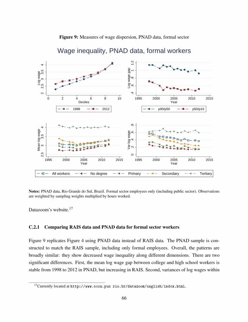
Figure 9: Measures of wage dispersion, PNAD data, formal sector2

2.5

33.

54

Log

wag

e

0 2 4 6 8 10Deciles

1998 2012

.4.6

.81

1.2

Log

wag

e ga

p

1995 2000 2005 2010 2015Year

p90/p50 p50/p10

2.5

33.

54

Mea

n lo

g w

age

1995 2000 2005 2010 2015Year

0.2

.4.6

.8V

ar lo

g w

age

1995 2000 2005 2010 2015Year

All workers No degree Primary Secondary Tertiary

Wage inequality, PNAD data, formal workers

Notes: PNAD data, Rio Grande do Sul, Brazil. Formal sector employees only (including public sector). Observationsare weighted by sampling weights multiplied by hours worked.

Datazoom’s website.17

C.2.1 Comparing RAIS data and PNAD data for formal sector workers

Figure 9 replicates Figure 4 using PNAD data instead of RAIS data. The PNAD sample is con-structed to match the RAIS sample, including only formal employees. Overall, the patterns arebroadly similar: they show decreased wage inequality along different dimensions. There are twosignificant differences. First, the mean log wage gap between college and high school workers isstable from 1998 to 2012 in PNAD, but increasing in RAIS. Second, variances of log wages within

17Currently located at http://www.econ.puc-rio.br/datazoom/english/index.html.

66

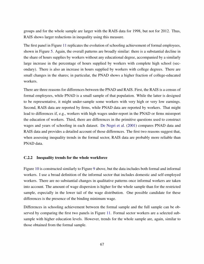
groups and for the whole sample are larger with the RAIS data for 1998, but not for 2012. Thus,RAIS shows larger reductions in inequality using this measure.

The first panel in Figure 11 replicates the evolution of schooling achievement of formal employees,shown in Figure 5. Again, the overall patterns are broadly similar: there is a substantial decline inthe share of hours supplies by workers without any educational degree, accompanied by a similarlylarge increase in the percentage of hours supplied by workers with complete high school (sec-ondary). There is also an increase in hours supplied by workers with college degrees. There aresmall changes in the shares; in particular, the PNAD shows a higher fraction of college-educatedworkers.

There are three reasons for differences between the PNAD and RAIS. First, the RAIS is a census offormal employees, while PNAD is a small sample of that population. While the latter is designedto be representative, it might under-sample some workers with very high or very low earnings.Second, RAIS data are reported by firms, while PNAD data are reported by workers. That mightlead to differences if, e.g., workers with high wages under-report in the PNAD or firms misreportthe education of workers. Third, there are differences in the primitive questions used to constructwages and years of schooling in each dataset. De Negri et al. (2001) compares PNAD data andRAIS data and provides a detailed account of those differences. The first two reasons suggest that,when assessing inequality trends in the formal sector, RAIS data are probably more reliable thanPNAD data.

C.2.2 Inequality trends for the whole workforce

Figure 10 is constructed similarly to Figure 9 above, but the data includes both formal and informalworkers. I use a broad definition of the informal sector that includes domestic and self-employedworkers. There are no substantial changes in qualitative patterns once informal workers are takeninto account. The amount of wage dispersion is higher for the whole sample than for the restrictedsample, especially in the lower tail of the wage distribution. One possible candidate for thesedifferences is the presence of the binding minimum wage.

Differences in schooling achievement between the formal sample and the full sample can be ob-served by comparing the first two panels in Figure 11. Formal sector workers are a selected sub-sample with higher education levels. However, trends for the whole sample are, again, similar tothose obtained from the formal sample.

67

Figure 10: Measures of wage dispersion, PNAD data, all workers2

2.5

33.

54

Log

wag

e

0 2 4 6 8 10Deciles

1998 2012

.4.6

.81

1.2

Log

wag

e ga

p

1995 2000 2005 2010 2015Year

p90/p50 p50/p10

2.5

33.

54

Mea

n lo

g w

age

1995 2000 2005 2010 2015Year

.3.4

.5.6

.7.8

Var

log

wag

e

1995 2000 2005 2010 2015Year

All workers No degree Primary Secondary Tertiary

Wage inequality, PNAD data, all workers

Notes: PNAD data, Rio Grande do Sul, Brazil. All employees (including public sector and informal sector). Observa-tions are weighted by sampling weights multiplied by hours worked.

C.2.3 Changes in relative labor supply

The first two panels of Figure 11, along with Figure 5 in the main text, show shares of hoursworked supplied by each schooling group. One might wonder whether these could reflect changesin selection patterns into employment over time (coming, e.g., from business cycle fluctuations)instead of changes in labor supply. The third panel in Figure 11 shows that this is not the case. Thatgraph shows the share of adults out of school, aged 18 through 54, in each educational group —regardless of whether they are employed, looking for jobs, or not in the labor force. The changes ineducational achievement from that figure are similar in magnitude to those in the second and firstpanels. The levels are different, though, suggesting selection into employment by education.

68

Figure 11: Changes in educational achievement, PNAD data

.1.2

.3.4

.5S

hare

of h

ours

wor

ked

1998 2000 2002 2004 2006 2008 2010 2012Year

Share of hours worked, PNAD, formal.1

.2.3

.4.5

.6S

hare

of h

ours

wor

ked

1998 2000 2002 2004 2006 2008 2010 2012Year

Share of hours worked, PNAD, all

0.2

.4.6

.8S

hare

of p

opul

atio

n

1998 2000 2002 2004 2006 2008 2010 2012Year

No degree Primary Secondary Tertiary

Adults by education group, PNAD

Notes: PNAD data, Rio Grande do Sul, Brazil. In the first two panels, the sample includesemployed workers and observations are weighted by sampling weights multiplied by hoursworked. In the third panel, the sample is composed of all adults 18-54 who are not in school,weighted by sampling weights.

69

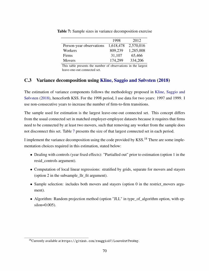
Table 7: Sample sizes in variance decomposition exercise

1998 2012Person-year observations 1,618,478 2,570,016Workers 809,239 1,285,008Firms 31,107 65,466Movers 174,299 334,206

This table presents the number of observations in the largestleave-one-out connected set.

C.3 Variance decomposition using Kline, Saggio and Sølvsten (2018)

The estimation of variance components follows the methodology proposed in Kline, Saggio andSølvsten (2018), henceforth KSS. For the 1998 period, I use data for two years: 1997 and 1999. Iuse non-consecutive years to increase the number of firm-to-firm transitions.

The sample used for estimation is the largest leave-one-out connected set. This concept differsfrom the usual connected set in matched employer-employee datasets because it requires that firmsneed to be connected by at least two movers, such that removing any worker from the sample doesnot disconnect this set. Table 7 presents the size of that largest connected set in each period.

I implement the variance decomposition using the code provided by KSS.18 There are some imple-mentation choices required in this estimation, stated below:

• Dealing with controls (year fixed effects): "Partialled out" prior to estimation (option 1 in theresid_controls argument).

• Computation of local linear regressions: stratified by grids, separate for movers and stayers(option 2 in the subsample_llr_fit argument).

• Sample selection: includes both movers and stayers (option 0 in the restrict_movers argu-ment).

• Algorithm: Random projection method (option "JLL" in type_of_algorithm option, with ep-silon=0.005).

18Currently available at https://github.com/rsaggio87/LeaveOutTwoWay.

70