Supply chain management simulation: an overviewCaroline Thierry, Gérard Bel, André Thomas. Supply...

HAL Id: hal-00321232https://hal.archives-ouvertes.fr/hal-00321232

Submitted on 1 Oct 2008

HAL is a multi-disciplinary open accessarchive for the deposit and dissemination of sci-entific research documents, whether they are pub-lished or not. The documents may come fromteaching and research institutions in France orabroad, or from public or private research centers.

L’archive ouverte pluridisciplinaire HAL, estdestinée au dépôt et à la diffusion de documentsscientifiques de niveau recherche, publiés ou non,émanant des établissements d’enseignement et derecherche français ou étrangers, des laboratoirespublics ou privés.

Supply chain management simulation: an overviewCaroline Thierry, Gérard Bel, André Thomas

To cite this version:Caroline Thierry, Gérard Bel, André Thomas. Supply chain management simulation: an overview.Caroline Thierry, André Thomas, Gérard Bel. Simulation For Supply Chain Management, ISTE andJohn Wiley & Sons, pp.1-36, 2008, Control Systems, robotics and manufacturing series. �hal-00321232�

https://hal.archives-ouvertes.fr/hal-00321232

https://hal.archives-ouvertes.fr

Chapter 1

Simulation for supply Chain management: An Overview

C. THIERRY, A. THOMAS, G. BEL

1.1. Supply chain management

In this book we are concerned with the simulation for Supply Chain Management (SCM): we focus on simulation approaches which are used to study the SCM practices [VOL 05].

The existence of several interpretation of SCM is a source of confusion both for those studying the concept and those implementing it. Indeed this term can expressed two concepts, depending on how it is used: Supply chain Orientation (SCO), is defined ([MEN 01]) as “the recognition by an organisation of the systemic, strategic implications of the tactical activities involved in managing the various flows in a supply chain”. Supply Chain Management is the “implementation of this orientation in the different member companies of the Supply Chain”.

1.1.1. Supply chain viewpoints

As said before, the main topic of this book is relative to simulation use for Supply Chain Management and Control. But to understand in what simulation can be useful for this objective, it is important to highlight the different issues of SCM, and to understand what a supply chain is or how many kind of SC can be considered. Thus, two viewpoints can be considered:

2 Titre de l’ouvrage

– the system under study is the supply chain of a given enterprise, and we can consider:

– the internal supply chain of an enterprise which focus on functional activities and processes and on material and information flows within the enterprise. In this case supply chain management may be viewed as the integration of previously separate operations within a business enterprise.

– the external supply chain of the enterprise which includes the enterprise, the suppliers of the company and the suppliers’ suppliers, the customers of the company and the customers’ customers (SCOR). In this case supply chain management mainly focuses on integration of operation and cooperation between the enterprise and the other actors of the supply chain.

– the supply chain under study is a network of enterprises (without a focus on one particular enterprise of the supply chain): a supply chain is a “network of organisations that are involved, through upstream and downstream linkages, in the different processes and activities that produce value in the form of products and services in the hands of the ultimate consumer.” ([CHR 92]). In this viewpoint, the focus is on the virtual and global nature of business relationships between enterprises. In this case supply chain management mainly focuses on cooperation between the supply chain actors.

1.1.2. Supply chain management

1.1.2.1. Supply chain processes: the integrated supply chain point of view

To describe supply chains with a process point of view, we refer to the Supply Chain Operations Reference (SCOR) model. SCOR is a cross-industry standard for supply chain management and has been developed and endorsed by the Supply-Chain Council (SCC). SCOR focuses on a given company and is based on five distinct management processes: Plan, Source, Make, Deliver, and Return.

Figure 1.1. The SCOR processes ([SCO 05])

Titre du chapitre 3

Supply chain management addresses different types of problems according to the concerned decision horizon. Long range (strategic) decisions are concerned with supply chain configuration: number and location of suppliers, production facilities, distribution centres, warehouses and customers, etc. Medium and short ranges (tactical and operational) are concerned with decisions material management: inventory management, planning processes, forecasting processes, etc.

On the other hand information management is also a key parameter of supply chain management: integrating systems and processes through the supply chain to share valuable information, including demand signals, forecasts, inventory and transportation etc.

Figure 1.2. which is adapted from the SSCP-Matrix [STA 00] synthesises the different supply chain decision processes:

SUPP

LIE

RS

Materialrequirement

Master scheduling

Distribution Planning

Purchasescheduling

Productionscheduling

Long term

Shortterm

Orderingmaterials

Shop floorcontrol

Warehousereplenishment

Demandfulfillmentand ATP

Mediumterm

Source Make Deliver Sale

Sale

s for

ecas

ting

and

dem

and

plan

ning

Transportscheduling

Distribution structure

Capacitybooking

Inventory level

Lot sizeLot size Transportation quantities and

modes

Start and finish dates for each

operation

Start and finish delivery dates

Start and finish transportation

dates

Sales & OperationPlanning

Capacitybooking

Inventory level

Purchasingquantities

Inventory level

Distribution network design

Supplynetwork planning

Master distribution

planning

Plant locationSuppliers selection

Production network design

CU

STO

ME

RS

Supplynetwork design

Figure 1.2. Different supply chain decision processes (1 organisational unit)


Supply chain management deals with the integration of organizational units. Thus the different supply chain processes will be more or less distributed according to the level of integration of the different processes.

1.1.2.2. Dynamic behaviour of supply chain management system

There is a process which organise the decisions at different level in the supply chain management system. This system (virtual world) is connected to the production system (real world) in order to compose a “closed loop” dynamic system.

SUPP

LIE

RS

Materialrequirement

Master scheduling


Purchasescheduling


Long term

Shortterm

Orderingmaterials

Shop floorcontrol



Mediumterm


Sale

s for

ecas

ting

and

dem

and

plan

ning

Transportscheduling


Capacitybooking

Inventory level


modes


operation



dates


Capacitybooking

Inventory level


Inventory level



Master distribution

planning



CU

STO

ME

RS


Figure 1.3. Dynamic behaviour of supply chain management system

Material flow Parts location

End of processing Time on a resource Inventory level

Scheduled receipts (End of planning period)

Inventory level Scheduled receipts (End of planning period)

Titre du chapitre 5

1.1.2.3. Supply chain processes: the collaborative supply chain point of view

Let’s now consider (figure 1.4) at least two independent organizational units (legal entities).

SUPP

LIE

RS

Materialrequirement

Master scheduling


Purchasescheduling


Long term

Shortterm

Orderingmaterials

Shop floorcontrol



Mediumterm


Sale

s for

ecas

ting

and

dem

and

plan

ning

Transportscheduling


Capacitybooking

Inventory level


modes


operation



dates


Capacitybooking

Inventory level


Inventory level




Master distribution

planning


CU

STO

ME

RS

Materialrequirement

Master scheduling


Purchasescheduling


Orderingmaterials

Shop floorcontrol




Sale

s for

ecas

ting

and

dem

and

plan

ning

Transportscheduling


Capacitybooking

Inventory level


modes


operation



dates


Capacitybooking

Inventory level


Inventory level





Master distribution

planning



Figure 1.4. Different supply chain decision processes (2 independent units))

In this collaborative supply chain, as far as a supplier-buyer partnership is established, several problems arise:

– how to exchange/share information? – is it possible to perform mutual problem solving? – how to set up global supply chains indicators?…

Thus the problem of the centralisation or distribution of the information and decision processes within the supply chain becomes a main challenge for the supply chain managers.

Material flow


1.2. Simulation for Supply Chain Management

1.2.1. Why to use simulation for Supply Chain Management?

As far as simulation is concerned the objective is to evaluate the supply chain performances. We distinguish tree ways to conduct Supply Chain performance measurement:

• analytical methods, such as queuing theory, • Monte-Carlo methods, such as simulation or emulation, • physical experimentations, such as lab platforms or industrial pilot

implementations. In this context of Supply Chain, analytical methods are impractical because the

mathematical model corresponding to a realistic case is often too complex to be solved. Obviously, physical experimentations suffer from technical- and cost-related limitations. Simulation seems the only recourse to model and analyse performances for such large-scale cases. Simulation enables, on the one hand, the design of the supply chain and on the other hand, the evaluation of supply chain management prior to implementation of the system to perform what-if analysis leading to the “best” decision. This simulation includes supply chain flows simulation and decision process dynamics. In the field of supply chain management, simulation can be used to support supply chain design decisions or evaluation of supply chain policies. As far as supply chain design decisions are concerned, the following decisions can be considered:

– Localisation - Location of facilities - Supply and distribution channel configuration - Location of stocks

– Selection - Suppliers - Partner

– Size - Capacity booking - Stock level…

As far as evaluation of supply chain control policies are concerned, the following decisions can be considered:

– Control policies - Inventory management, control policies - Planning processes

– Collaboration policies

Titre du chapitre 7

- Cooperation/collaboration/coordination… - Information sharing…

1.2.2. How to use simulation for Supply Chain Management?

To attempt to specify the different ways to use simulation for SCM it is important to differentiate, on the one hand, the real system (the “real world”) and on the other, its simulation model.

In fact, the simulation model must be built according to its usage and/or the SCM function that we want to model or to evaluate. Different classes of models can be highlighted to understand the variety of SC simulation models according to:

– the systemic decomposition of the SCM system - Decision system - Information system - Physical system

Figure 1.5. Systemic decomposition of the SCM system

– the level of distribution of the system: - simulation model for centralized SCM system evaluation

A centralised SCM system consists in a single information and decision system for the different entities of the supply chain under study.

- simulation model for distributed SCM system evaluation A distributed SCM system consists in a distribution of the decision system

over different entities of the supply chain under study.

As a matter of fact, the execution of the simulation can be performed: - In a centralised way on a single computer

Physical system (parts, resources, …)

Real stateDecision

Information system

Decision system (Hierarchical Planning and

control process)

Real state Decision


- In a decentralised way: - on multiprocessor computing platforms : parallel simulation - or on geographically distributed computers interconnected via a network,

local or wide: distributed simulation.

As far as decentralisation of the simulation is concerned, “the execution of a single main simulation model, made up by several sub-simulation models, which are executed, in a distributed manner, over multiple computing stations”. [TER 04]

The need of a distributed execution of a simulation across multiple computers derives from four main reasons [TER 04]:

– to reduce execution simulation time […] – to reproduce a system geographic distribution […] – to integrate different simulation models that already exist and to integrate

different simulation tools and languages […] – to increase tolerance to simulation failures […]” – to test independently different control models – to progressively deploy a control system, – to prepare at SC control changes” More over it is important to stress that simulation mostly focuses on the

dynamics of the supply chain processes concerning both physical and decision systems (i.e. production management systems see §1.3.1.).

1.3. Supply chain management simulation types

This section is dedicated to the presentation of the different types of models and approaches mainly used for supply chain management simulation.

As seen before, an important part of the model is the decision system model (hierarchical planning and control processes). So the first subsection presents the main production management models which are used in supply chain management.

Then, the different kinds of well known simulation models will be quickly presented. For each of them we will highlight how the different production management models can be linked with the simulation model.

1.3.1. Production management models focus

The objective of this part is to focus and to present a very synthetic and simplified description of production management models in order to introduce, in a following part, how they can be integrated in a supply chain simulation model. Here

Titre du chapitre 9

we focus only on the production processes even the approach could be extended to supply and distribution processes.

There are two main categories of production management models.

1.3.1.1 Time bucket models

In production planning and control, and mainly for long and middle term, we are concerned with the determination of quantities to be produced per time period for a given horizon in order to satisfy demand or/and forecast. To perform these decision processes, time bucket models are needed. They are characterized by:

– Decision variables: produced, stocked or transported quantities – Data: capacities of the resources (in number of parts per period, for example) – Constraints: conservation of flow, bill of materials, limited capacities, demand

satisfaction… Example: For a production line composed of two production resources (see figure 1.6.).

Figure 1.6. Time bucket model (example)

The demand is dt and the production resources capacities are CR1,t, CR2,t. Each item is produced from one single component.

The planning model variables are: - xRi,t= quantity of items to be produced on resource Ri during time period t - yRi,t= quantity of items to be transported from resource Ri during time

period t - IiRi,t= input inventory level on resource Ri at the beginning of time period t. - IoRi,t= output inventory level on resource Ri at the beginning of time period t.

The planning model constraints are: - Ii R1,t+1 = IiR1,t - x R1,t - IoR1,t+1 = IoR1,t + x R1,t - yR1,t

StockProduction Stock

R2

ouput inventoryIR2,t

Production(xR1, t)

ouput inventory IoR1,t

R1

Production(xR2,t)

input inventory IiR1,t

input inventoryIiR2,t

Transportation(yR1,t)



- Ii R2,t+1 = IiR2,t - x R2,t + yR1,t - IoR2,t+1 = IoR2,t + xR2,t – yR2,t - y R2,t = d t - xR1,t ≤ CR1,t - xR2,t ≤ CR2,t - Ii R1, t0= ∞ - IiR, t ≥ O ∀R∈{R1, R2}, ∀t - IoR, t ≥ O ∀R∈{R1, R2}, ∀t - xR,t ≥ 0 ∀R∈{R1, R2}, ∀t - yR, t ≥ 0 ∀R∈{R1, R2}, ∀t

Joint to these models, methods are used to perform the plan: MRP like methods,

mathematical programming, constraints programming, meta-heuristics.

1.3.1.2. Starting time models

In production planning and control, and mainly for short term, we are also concerned with the determination of the starting time of tasks on different resources. For that we use starting time models (sequence of timed events). These models are characterised by:

– Decision variables: starting time of tasks (ti) – Data: ready dates (ri,) due dates (di) – Constraints: precedence, resource sharing, due dates Example:

- ti ≥ ri - ti ≥ tj + pj OR tj ≥ ti + pi

- ti + pi ≤ di

Joint to these models, methods are used to perform the schedule: mathematical programming, constraints programming, meta-heuristics…

1.3.2 Simulation types

Due to the special characteristics of supply chains, the supply chain simulation model building is difficult. The two main difficulties are highlighted, and then the different types of models for supply chain management simulation are quickly presented.

Titre du chapitre 11

1.3.2.1. Size of the system

One characteristics of supply chain simulation is the huge number of “objects” to be modelled. A supply chain is composed of a set of companies, composed of a set of factories and warehouses, composed of a set of production resources and stocks. Between all these production resources circulate a set of components, parts, assembled parts, sub-assemblies and final products. So the number of “objects” of the model can be very large.

1.3.2.2. Complexity of the production management system

To simulate a system it is necessary to simulate the behaviour of the “physical” system and the behaviour of the “control” system. For a supply chain this implicates that it is necessary to model the behaviour of the supply chain management system of each company and the relation between these production management systems (cooperation).

As this supply chain management system is very complex, it can be difficult to model it in details. However it is absolutely necessary to model it, as it is this system which controls the product flow in the supply chain. So, according to objective of the simulation study and the kind of chosen model, various aggregated or simplified models of the production management system must be designed. Following sections present different examples of these models.

1.3.2.3. Different kinds of models for supply chain management simulation

1.3.2.3.1 Simulation model

A simulation model is composed of a set of “objects” and relations between these objects; for example: in a supply chain main objects are items (or set of items) and resources (or set of resources).

Each object is characterised by a set of “attributes”. Some attributes have a fixed value (example: name) others have a value which varies during the time (example: position of an item in a factory).

The state of an object at a given time is the value of all its attributes. The state of a system at a given time is the set of the attributes of the objects included in the system.

The purpose of a simulation model is to represent the dynamic behaviour of the system.

There are various modelling approaches according to how state variations are considered:

- States vary continuously: continuous approach - States vary at a special time (event): discrete event approach.


The following parts of this section will introduce the chapters 2 to 4 which will go into details on the viewpoint and present related works (State of art and recent works).

1.3.3. Simulation of supply chain management using continuous simulation approach

In this section we will introduce system dynamics, a continuous simulation approach where states vary continuously. Chapter 2 will go into details and present recent works related to this viewpoint of simulation for supply chain management. 1.3.3.1. System dynamics

This new paradigm has been first proposed by Forester for studying “Industrial Dynamics”.

Companies are seen as complex systems with [KLE 05] : – different types of flows: manpower, technology, money, and market flows. – stocks or levels which are integrated into time according to the flow

variations System dynamics is centred on the dynamics behaviour. It is a flow model where

it is not possible to differentiate individual entities (like transport resources). Management control is performed by making variations on rates (production

rates, sale rates,…). Control of rates can be viewed as a strong abstraction of common production management rules.

The model takes into account the “closed loop effect”: the manager is supposed to compare continuously the value of performance indicator to a target value. In case of deviation he implements corrective actions.

Example: - It2 = It1 + p(xr t1,t2 – drt1,t2) - xr t1,t2 = production rate between two dates t1 and t2 - dr t1,t2 = sale rate between two dates t1 and t2 - p = time duration between t1 and t2

1.3.3.2. Production management models/ simulation models

The two models do not consider the same objects states. – In systems dynamics objects are continuous flows. The behaviour of these

flows are represented by a differential equation (with derivate) which is integrated using a time sampling approach.

– In planning models the objects are resources and their activities. It is considered that the attributes of these activities change only at a special periodic dates. There is no notion of derivate.


This kind of model seems well adapted to supply chain simulation as it has been design by Forester for “Industrial Dynamics” studies which used same concepts as those used lately in supply chain studies.

1.3.4. Simulation of supply chain management using discrete event approach

In this section we will detail the discrete event approach. We will distinguish between time bucket driven approach and even driven approach. This differentiation is based on the time advance procedures which characterized these two approaches. Chapter 3 will go into details and present recent works related to this viewpoint of simulation for supply chain management. For the “discrete event approach” they are:

– different ways to “see the world”: activities, event and process

event

activity

process

time

event

activity

process

time

Figure 1.7. Events, activities, processes

– different procedures to make the time advance in the simulation: - event driven

time

event event event event

timetime

event event event event

Figure 1.8. Event driven discrete events simulation

- time bucket driven


time

Activityevent event

Time bucket Time bucket Time buckettime

Activityevent event

time

Activityevent event

Time bucket Time bucket Time bucket

Figure 1.9. Time bucket driven discrete events simulation

The main practices to “mix” various types of models and time advance procedures are listed below:

X

x

events

XxNot possible with the

approach

Event driven

xXXTime bucket driven

processactivitiescontinuous

X

x

events

XxNot possible with the

approach

Event driven

xXXTime bucket driven

processactivitiescontinuous

Figure 1.10. Discrete events simulation

1.3.4.1. Time bucket driven approach

Discrete events simulation using time bucket driven approach is rarely used for job shop simulation but it well fits for simulation of supply chain management (see the specific characteristics of this simulation in §1.3.2.1 and §1.3.2.2).

1.3.4.1.1. Time bucket driven discrete events models

In such a model: – time is divided in periods of a given length: time bucket – time is incremented step by step with a given time bucket. At the end of each

step a new state is calculated using the model equations. So in this approach it can be considered that events (corresponding to a change of the state) occur at each beginning of a period

– the lead time for an item on a production resource is considered small compared to the size of the time bucket

– the main states are the states of resources (or set of resources) during a given period: they describes the activities in which resources are implicated in a given


time period. They are characterised by the quantities of items processed in this activity in a given time period: for example the number of items of a given type manufactured, stocked or transported by a given resource in a given period.

– the simulation has to determine all the states of all the resource at each period of a simulation run.

This kind of model is also called “Spreadsheet simulation” [KLE 05]. We don’t adopt this designation because spreadsheet is a tool with which it is possible to use all the modelling approach.

1.3.4.1.2. Simulation models

It must be noticed that the planning models presented in § 1.3.1 are also time bucket models which are well known and used in production management domain. We will see hereafter that they are very similar to time bucket driven discrete events simulation models but that they are used in a different way in simulation.

In order to illustrate that, we consider a very simple example of a production line composed of two production resources with no specific production management. Shop floor control is a first-in first-out strategy, k is the number of parts from M1 to be used to produce one part on M2.

Figure 1.11. Production management models/ simulation models (example)

The simulation model uses the following state variables: - IiRi,tis the input inventory level of resource Ri at the beginning of time

period t. - IoRi,tis the output inventory level of resource Ri at the beginning of time

period t.

Production

M1 M2

ouput inventory

IR2,t

Production(xR1, t)

ouput inventory

IoR1,t

M1 M2

Production(xR2,t)

input inventory

IiR1,t input

inventoryIiR2,t


Shop floor control


- xRi,t is the quantity of part produced by resource Ri during the time bucket t (available at the end of t)

- yRi,t is the quantity of parts transported from Ri during time bucket t (available at the end of t)

The model of the dynamic behaviour of the system is the following: - Ii R1,t+1 = IiR1,t - x R1,t - IoR1,t+1 = IoR1,t + x R1,t - yR1,t - Ii R2,t+1 = IiR2,t - x R2,t + yR1,t - IoR2,t+1 = IoR2,t + xR2,t - yR2,t

- xR1,t ≤ CR1,t - xR2,t ≤ CR2,t

It can be noticed immediately that this model is very similar to the production management model presented in § 1.3.1.1.

In order to illustrate that, let’s consider a simulation with this model corresponding to the following hypothesis: resource R1 sends parts to resource R2 according to a production and transportation plan determined outside of the system. So IiR1,t0, IiR2,t0, xR1,t,, xR2,t, yR1,t, yR2,tare known at the beginning of the simulation.

In this case, the true state variables of the model are IiR1,t, IiR2,t , IoR1,t, and IoR2,t.

The simulation must determine the variation over time of this variables taking into account the values of the exogenous variables (xR1,t,, xR2,t, yR1,t, yR2,t). Thus simulation allows evaluation of the proposed production and transportation plan. It is also possible to introduce hazard in the behaviour of the model.

Figure 1.12. Simulation process

This shows that the same model can be used in a: – simulation decision process: taking into account xR1,t xM2,t, yR1,t and yR2,t.. the

problem is to determine IiR1,t, IiR2,t , IoR1,t, and IoR2,.

– production planning decision process: in a centralised planning (APS or SCM like) the problem is to determine xRi,t and yRi,t which satisfy the constraints of the planning model (stock capacity, supplier demand ).

y Simulation

Aléas

R2,t

R2,t SimulationIi

Perturbations

Ri,t Ri,tIo Ii y R1,t

x R1,t x

R1,t0


Notice: it is possible to use a “what if” approach with the planning model testing different demands or different production management policies. In this “what if” approach the problem is solved several times, each time with this different data. Then it is possible to see the influence of these data on the generated plan. This approach is not considered in this book: we refer to simulation only when the dynamics of the system is considered.

1.3.4.1.3. Production management models/ simulation models

Now the question is: how the different production management models can be linked to a discrete events simulation model with time bucket approach?

Time bucket production planning model can be easily linked to the global simulation model as the modelling approach is the same. In this case the two models will be joined up: the simulation model focuses on the circulation of the flow of parts, the planning model determines the quantities to be produced. The Chapter 3 provides a study of both discrete events and time bucket simulation used for supply chain management and proposes case studies to illustrate the pivotal role that simulation can play as a technique for decision aid.

If we consider now the other category of production management models that we call in § 1.3.1.2 “starting time models” (scheduling,…) we can state that:

- “time bucket driven discrete events simulation models” do not use the same “objects states” than “starting time production management models” (which use “start time of an activity”).

- between two periods the bucket driven activities simulation model does not represent the state of the system. So the start time of an activity is not known and cannot be used as data in a “starting time” scheduling model. The only way to obtain a good approximation of this date can be to use a very small time period. But this is often not possible because this will contradict the fundamental hypothesis for this kind of model: the production duration for an item on a production resource is very less than the time bucket of the model.

1.3.4.2. Event driven approach

In this sub-section the main characteristics of the discrete events models for supply chain management simulation using event driven approach is presented. Remember that this approach is intensively used for job shop simulation. So it can be consider as convenient to use this kind of model for supply chain simulation.


However using the specific characteristics of supply chain management simulation (see §1.3.2.1 and §1.3.2.2) can induce some difficulties for this kind of simulation. The main difficulty comes from the size of the model induced by this context. It can be not efficient to model the circulation of each individual part in each production resource of the different companies of the supply chain: the number of events can become prohibitive and slow down considerably the simulation which can become unworkable. It is why it is often necessary to use model reduction techniques introduce here after §1.5.2. As seen before, chapter 3 provides a study of both discrete events and time bucket simulation used for supply chain management and proposes case studies to illustrate the pivotal role that simulation can play as a technique for decision aid. We remind hereafter the main characteristics of this approach.

1.3.4.2.1. Event driven approach for discrete events simulation

In a event driven discrete events model: – the main states are the states of items (or set of items) – the simulation must determine the dates of all the events (state variation) which

occurs during a simulation run – each state is characterised by the resource utilised by a given item at a given

time and correlatively the “occupation state” of the resources. Example: position of a given item (“on a given production resource” , “in a given stock”, or “being transported by a given cart”)

– each state variation is represented by a “state variation logic” – time advance event to event. A “simulation engine” using “ a “time table”

determine the date of the “next event” (ex: the delivery date of a job).

1.3.4.2.2. Production management models/ simulation models

Consider again the question which is to know how the different planning models can be connected in a event driven discrete events simulation?

The time buckets planning models cannot be directly connected to an event driven discrete events simulation because the modelling approach is not the same. We will see chapter 3 how different adaptations can be realized in order to allow connections.

The “starting time models” presented in §1.3.1.2 (scheduling level) can be directly connected to an event driven discrete events simulation because they use the same modelling approach.

In summary for this event driven approach:


- Simulation models and planning models does not use the same “objects states”.

- Simulation models and scheduling or shop floor control models use the same “objects states”

1.3.5. Simulation of supply chain management using games

In this section we will introduce the business games then chapter 4 will go into details and present recent works related to this viewpoint of simulation for supply chain management.

1.3.5.1. Games and simulation

Different games can be used to perform simulation. Games enable simulating real conditions off-line, and exploring new ideas or strategies in a safe, interactive and also fun environment. Basically, the complexity of their model allows splitting games into two classes:

– board games have a model simple enough to be played with tokens or pieces that are placed on, removed from, or moved across a "board" (a premarked surface, usually specific to that game).

– sophisticated games have a more realistic model requiring, for example, to be run on computerized devices.

1.3.5.2. Production management models/ simulation models

In this kind of simulation model (board games), the simulation of time can be made using either a clock which synchronises the players, or the time of the simulation is the real time (each player evolves independently). [KLE 05] distinguishes:

– Strategic games: in these games every player represents a company competing or collaborating through other companies by interacting with the simulation model during several rounds. The well-known beer game belongs to this category.

– Operational games: in these games every player represents an actor (e.g. a worker of a workshop) interacting with the simulation model either during several rounds or in real time. Examples include games for training in production scheduling.

1.4. Decision systems and simulation models (systems)

The preceding sections have presented the main concepts which are used in supply chain management simulation and introduce the first part of the book (chapter 2 to 4).


The second part of the book is dedicated to the problem of distribution of the supply chain management simulation. This concept of simulation distribution is extremely important in the case of supply chain simulation because of the naturally distributed aspect of the supply chain by its elf. This section introduces this part of the book (chapter 5 to 10).

1.4.1. Models and system distribution

There is a consensus on the architecture of simulation environments putting the emphasis on modularity between the control system CS and the shop-floor system SF. This separation principle enables to introduce the concept of emulation. Emulation is not new, it is used in automation to test computer aided manufacturing software, for example [COR 89]. Fusaoka proposed a theoretical formulation and an experimental run consisting in verifying the assertion SF∧CS⊃G [FUS 83], where G is the required performance level of the shop floor. The real shop floor system (SFr) may be replaced by a model (SFm) , that we call an emulated shop floor. Likewise, a model of the control system (CSm) can be used instead of the real one (CSr). Therefore, four experimental situations can be defined, using either models or real systems [PFE 03]:

1. (SFr, CSr) Experimentation consists in deployment of the real control system at the Shop floor. It is the more classical case.

2. (SFr, CSm) A Control system model is applied for the real shop floor. This configuration could be used to test a new control system.

3. (SFm, CSr) The real control system is used with a shop floor model (emulation with the real control system)

4. (SFm, CSm) Both shop floor and control system are modelled.

Let’s first focus on a single company of the supply chain or on a centralized SCM system. The real system is made up of the physical system, the information system and the control (or decision) system (Cases 1 and 4 on Figure 1.13). These three systems compose the SCM system. Basically, building a simulation model leads to design a virtual model representation of these (or at least one of these) three preceding systems implemented on a computer S1, as seen in §1.3.


Productioneventsreports

Productionexecution

actions


Control SystemOn computer R1 in real time

connected to Physical and Information Systems

withHierarchical Decision making process

Information SystemOn computer R1

in real time connected to physical and control Systems

Physical System(items, resources, …)

Decisions

Productionexecution

actions

Real System


Productionexecution

actions


Control System ModelOn computer S1 in real time



Information SystemOn computer S1


Physical System Model(items, resources, …)

Decisions

Productionexecution

actions

Real System simulation ModelOn computer S1

Figure 1.13. Real time Simulation Model

Let’s now consider different cases where this model can be distributed.

If we want to evaluate the effect of different control rules, on a specific physical system, it could be interesting for example to build an emulation system corresponding to this physical system. This emulation model being controlled by the real decision System (Case 3 on Figure 1.14.) connected to the actual information system. Actually, emulation aims at mimic the behaviour of the physical system only. It can be seen as a virtual shop floor which can be connected to an external control system. Like simulation, emulation can be used to model complex cases, but emulation remove the additional task of modelling decision processes (this task being often one of most difficult as stated by [VAN 06] and presented here before § 1.3.2.2).



Productionexecution

actions







Physical System(items, resources, …)

Decisions

Productionexecution

actions

Real System


Productionexecution

actions



connected to emulation and Information Systems




Physical System Model(items, resources, …)

Decisions

Productionexecution

actions

Real System emulation ModelOn computer S1

Real System

Figure 1.14. Emulation system connected to real control system

Using emulation provide modularity between tests cases and control systems to be tested. This modularity is useful to try a control system in various situations, or to try various control systems on a same test case. It can also be useful to validate the real control system before actually deploying it.

Obviously, the same concept can be use for a Supply Chain System (Figure 1.15. and 1.16.). But, Supply Chain being networks of companies often independents (i.e.§ 1.1.1.) , simulation models can be built in a centralised way (Figure 1.15.) or in a distributed way (Figure 1.16.). In a distributed context, different simulation models can be implemented on different computers, each one representing companies’ behaviour.



Productionexecution

actionsProduction

eventsreports

Control System AOn computer R1 in real time



Information System AOn computer R1


Physical System A(items, resources, …)

Decisions

Productionexecution

actions

Real System – Company A


Productionexecution

actionsProduction

eventsreports

Control System BOn computer R1 in real time



Information System BOn computer R1


Physical System B(items, resources, …)

Decisions

Productionexecution

actions

Real System – Company B

Parts

Information

Real Supply Chain


Productionexecution

actionsProduction

eventsreports

Control System Model AOn computer R1 in real time



Information System Model AOn computer R1


Physical System Model A(items, resources, …)

Decisions

Productionexecution

actions



Productionexecution

actionsProduction

eventsreports

Control System Model BOn computer R1 in real time



Information System Model BOn computer R1


Physical System Model B(items, resources, …)

Decisions

Productionexecution

actions


Parts

Information

Centralized simulation Model of a Supply Chain on a computer S1

Figure 1.15. Centralized Supply Chain Simulation Model


Productionexecution

actionsProduction

eventsreports

Control System AOn computer R1 in real time



Information System AOn computer R1


Physical System A(items, resources, …)

Decisions

Productionexecution

actions



Productionexecution

actionsProduction

eventsreports

Control System BOn computer R1 in real time



Information System BOn computer R1


Physical System B(items, resources, …)

Decisions

Productionexecution

actions


Parts

Information

Real Supply Chain


Productionexecution

actionsProduction

eventsreports

Control System Model AOn computer R1 in real time



Information System Model AOn computer R1


Physical System Model A(items, resources, …)

Decisions

Productionexecution

actions



Productionexecution

actionsProduction

eventsreports

Control System Model BOn computer R1 in real time



Information System Model BOn computer R1


Physical System Model B(items, resources, …)

Decisions

Productionexecution

actions


Parts

Information

Centralized simulation Model of a Supply Chain on two computers S1 and S2

Figure 1.16. Distributed simulation models of a Supply Chain


As underlined in the preceding sections, SC management systems are traditionally organised in a hierarchical way. Different decision functions exist: Planning, Master Scheduling, detail scheduling and Control according to the classical MRP² System describe by [VOL 05]. This kind of architecture exists in each company belonging to the SC. In internal SC, the same ERP software could be used, but in external one, often different information and decision systems ERP must be connected, leading to interoperability problems and/or synchronization problems.

The following parts of this section will introduce the chapters 5 to 10. These different chapters will describe respectively simulation problems relative to centralized architectures, simulation synchronization problems and distributed simulation architectures.

1.4.2. Centralized simulation

The decisions that are usually taken before planning on the implementation of any supply chain can be classified into two categories: structural (for long term objectives) and operational (for short term goals). Simulation can be used as a tool for carrying out the decision making process for both structural and operational decisions thanks to dynamic simulation of material flow and taking into account of all random phenomena. In opposite of distributed simulation, in a centralized approach, one single simulation model reproduces all the supply chain structures (entities and links).

The chapter 5 is dedicated to this kind of approach. It presents a brief literature review on supply chain centralized simulation and discusses on two developed centralized simulation approaches. Effectively, for most simulation evaluation approaches, supply chain processes are modeled to perform “what-if” analysis. Firstly, a discrete-event simulation-based optimization is used to estimate the operational performances of the solutions suggested by the optimizer. The optimizer was developed based on the NSGA-II, which is considered one of the best multi-objective optimization using a genetic algorithm [DEB02].

Moreover this chapter 5 illustrates the applicability and efficiency of the two preceding approaches using three industrial applications. In the first one, a case study from automotive industry will be presented. The objective is to improve the profitability and responsiveness of the company’s supply chain by redesigning its production-distribution network. A centralized simulation-based optimization approach is used for the optimization of facility open/close decisions, production order assignment and inventory control policies. In the second case, the authors applied the centralized simulation-based multi-objective genetic algorithm approach to a real-life case study of a multi-national textile supply chain, which consists of several suppliers, a single distribution center and an aggregated customer. The modeling and simulation details are discussed and numerical results are presented analyzed. In the third case, another automotive industry case, a generic model is


proposed, which can be used by different automotive industries. The developed model is limited to only the interactions between the assembly line and its direct suppliers. Taking into account that the model is generic, it is able to help supply chain decision-makers in their choices.

1.4.3. Multi Agents Systems decision simulation

New forms of organizations have emerged from Supply Chain concept in which partners have to collaborate and have strong collaboration. Producing enterprises operate as nodes in a partner network and share activities to produce and deliver theirs goods. In such context, integration of planning of all the nodes is needed, that is to say, that partners have to be able to distribute and synchronize their activities.

To obtain the optimal performance level in such dynamic environment, multi-agents Systems (MAS) can be used. Effectively, MAS are composed (as a Supply Chain network is) of a group of agents that can take specific roles within the organizational structure. Different agents may represent different objects belonging to the studied network. This idea is not new; Parunak used agents for manufacturing control or collaborative design ([PAR 96] or [PAR98]) nevertheless these approaches are particularly well adapted when studying supply chain management.

Chapter 6 and 7 are dedicated to MAS usage for SCM. The first one highlights the interest to use MAS for Supply Chain simulation and the second one, considers MAS decisional system simulation for enterprise network.

Just like a Supply Chain in which distributed activities and decisions are made in order to obtain a global optimal performance, MAS simulation leads to a distributed system, within there is generally no centralized control, to have a global point of view; where agents act in an autonomous way and do not have locally the global knowledge, to obtain nevertheless a global optimum. Effectively, several analogies between Supply Chains and MAS can be highlighted:

• The multiplicity of acting entities • The entities properties, abilities or decision-making capabilities… • Information sharing and task distribution…


A review of research works on agent-based supply chains modelling and simulation is also made in chapter 6. On the other hand, chapter 7 presents specific contributions in agent-based Supply Chains modelling and simulation for decision system development. The first part of this chapter will concern the Supply Chain control, and the second one, is related to the design of decision system based on simulation.

1.4.4. Simulation for Product Driven Systems

As said before, in the distributed Supply Chain and manufacturing control context, Multi agent Systems (MAS) are often used according to the fact that each company could act, in some circumstances, in an autonomous way. Consequently, it is possible to implement agents to describe their behaviour. Thus, the SCM System could be composed by planning and scheduling agents and by agents representing physical elements as products, for example.

Moreover, it is also possible to built emulation model for distributed supply chains. This kind of model can be made in a centralized or distributed way (using several models and computers for physical, control and decision systems). This last possibility is interesting for all contexts where products and/or physical entities are able to take some autonomous decisions. The main idea, is to focus the decision-making processes as near as possible to the shop-floor or physical system, where events (disturbing or not) actually occurs. Current researches focusing on autonomy are for instance Holonic Manufacturing Systems (HMS), multi-agents based control, or more generally intelligent manufacturing. These take their roots both in fundamental research such as distributed artificial intelligence, artificial life or cooperative control, and also in practical experiences such as kanban-controlled systems, or empowered operators.

Centralised control systems showed their limits to efficiently respond to frequent changes, which led researchers on the way of distributed manufacturing systems ([DIL 91]). But advances in this domain show limitations with systems stability’s and global optimisation.

The qualities and complementarities of both centralised and distributed approaches (hybrid architectures) let foreseen considerable benefits of coupling them together, adding the global optimisation abilities from centralised control systems with the reactivity and the possible robustness of decentralised ones. Both hierarchical and heterarchical approaches share benefits and drawbacks. As a consequence has emerged the idea of coupling both systems, with the aim of ensuring a global optima while keeping the heterarchical systems reactivity. This concept would be realistic by using such technologies as RFID. This technology


enabled to postulate that embedding intelligence into the product could lead to some types of product-driven systems. ([WON02])([MOR 03]).

This concept need to use in a different way simulation, especially, the simulation tool must reproduce the “communicant product” behaviour. Consequently, the simulation tool is built in two parts, the first one, is an “emulation model” where the entities represent items and don’t have any attributes (no information and decision are implemented in the model), and the second one, is a “control model” where the entities represent an information flow activated by events occurring in the emulation model.

Informationalsystem

DecisionalSystem

Control Model

Communication interface

Node 1Node 2Create Dispose

Synchronisation pointsEmulation Model

Figure 1.17. Product Driven System Simulation

As shown previously, assessing the impact of synchronising physical and informational flows needs to model them as distinct flows (figure 1.17.). In that way, it could be interesting to represent them in two distinct models, that works simultaneously and have to be synchronised. Moreover, the interface standardisation enables to exchange different control models with the same physical emulation one. To represent the implementation of RFID technologies, with fixed readers, the notion of synchronisation points is implemented in the model, which are points where the physical system emits events to update the information system. This event update could launch a decision process that will react by acting on the emulation model. Chapter 8 will be dedicated to this concept.

1.4.5. Models synchronisation = HLA distributed simulation approaches

To face flexibility and reactivity SC problems, recent researches consist in developing adapted simulation environments, allowing the analysis and the evaluation before considering an operational deployment. In a Supply Chain context, we can imagine that building a unique SC model could be a very difficult task, that could lead to simplifying, to strong hypotheses and finally to unrealistic results.


Moreover, running such a model could lead to data problems. As a result, there is a real need for Distributed Simulation (DS) in SCM. That is to say, that a unique control system could manage several physical systems simulation models (Figure 1.18.) or that is to say that such an implementation needs a communication protocol allowing the exchange of information between the various components.

The appearance of standards of distributed simulation specification allows facilitating the implementation of such simulations. A treatment in distributed simulation must be ensured to respect the existing causality relations. Moreover, it is important to take into account all events arising as the time go on, that is to say, it is important to manage the time. Indeed, the problems of messages coordination between the partners of the supply chains and of synchronization of these partners must be managed. The chapter 9 will presents various techniques of existing distributed modelling and simulation (DEVS (Discrete Event system Specification), SIMBA (Simulation Based Applications), HLA (High Level Structures)) by exposing the characteristics.

To have a no ambiguous description of the system and to have a definition of discrete events simulation algorithms whose validity is founded and verifiable, DEVS and SIMBA formalisms can be useful to obtain models formal specification. The American defence has developed the HLA (High Level Architecture) protocol in order to synchronize within a great simulation, simulators being carried out on different computers.

Figure 1.18. Multi-lines synchronization problems

This chapter 9 relates to the study of the multi-lines synchronization problems in internal logistic. Emulation and control models will be presented. Following this


study is illustrated by an industrial case. This application takes into account two production sites containing several lines of assembly. HLA ensures interoperability between these various models.

1.5. Simulation software

To evaluate decision impact or to choose a management production or Supply Chain organisations, it is today natural to use simulation. Law and Kelton [LAW 91] summarise several reasons for the spectacular increase in the use of simulation in the field of manufacturing and Supply Chain systems. Consequently, we can find today a lot of relevant simulation software, more and more used according to the complexity inherent of the Supply Chain problems.

The main goal of the chapter 10 is to highlight simulation software functionalities. Firstly, a software typology will be proposed. This typology is establish, for discrete-events simulation, according to some literature criteria as event, activity or process approaches, etc… Secondly, supply chain test games will be presented. They are described by a knowledge model and particular formalism that will be explained. These test games are useful to choose or to analyse different simulation software. Finally, a special methodology will be proposed to help modeller to specify his needs and to choose his simulation tool.

1.6. Simulation methodology

1.6.1. Evaluation of simulation models

The simulation model quality evaluation is a hard problem. It isn’t possible to do that in a formal way (especially for discrete events simulation). At least, we want to have a model behaviour leading to obtain simulation measure indicators values, as close as possible, than the same indicators measures on the real system. As we said previously, the model contains always approximations due to necessary simplifications. Thus, to evaluate this quality, we have to focus on the simulation system architecture, on the one hand, and on its proposed results (indicators), on the other.

Two criteria concern the study of reference architecture quality: – the first one concerns the architecture structural proprieties (nature of

information, use and implementation easiness, reusability, etc.. ) – the other one concerns the operational performances of the simulation model.


It’s possible to study the structural aspects through a theorical approach, without any application. But on the other hand, operational performances must be evaluated by simulation runs.

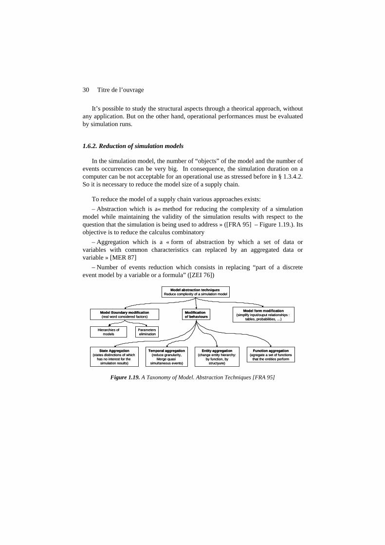
1.6.2. Reduction of simulation models

In the simulation model, the number of “objects” of the model and the number of events occurrences can be very big. In consequence, the simulation duration on a computer can be not acceptable for an operational use as stressed before in § 1.3.4.2. So it is necessary to reduce the model size of a supply chain.

To reduce the model of a supply chain various approaches exists: – Abstraction which is a« method for reducing the complexity of a simulation

model while maintaining the validity of the simulation results with respect to the question that the simulation is being used to address » ([FRA 95] – Figure 1.19.). Its objective is to reduce the calculus combinatory

– Aggregation which is a « form of abstraction by which a set of data or variables with common characteristics can replaced by an aggregated data or variable » [MER 87]

– Number of events reduction which consists in replacing “part of a discrete event model by a variable or a formula” ([ZEI 76])

Model abstraction techniques Reduce complexity of a simulation model

State Aggregation(states distinctions of which

has no interest for thesimulation results)

Temporal aggregation(reduce granularity,

Merge quasi simultaneous events)

Entity aggregation(change entity hierarchy:

by function, by structyure)

Function aggregation(agregate a set of functions

that the entities perform

Model Boundary modification(real word considered factors)

Model form modification(simplify input/ouput relationships :

tables, probabilities, …)

Modification of behaviours

Hierarchies of models

Parameterselimination

Model abstraction techniques Reduce complexity of a simulation model

State Aggregation(states distinctions of which

has no interest for thesimulation results)

Temporal aggregation(reduce granularity,

Merge quasi simultaneous events)

Entity aggregation(change entity hierarchy:

by function, by structyure)

Function aggregation(agregate a set of functions

that the entities perform

Model Boundary modification(real word considered factors)

Model form modification(simplify input/ouput relationships :

tables, probabilities, …)

Modification of behaviours

Hierarchies of models

Parameterselimination

Figure 1.19. A Taxonomy of Model. Abstraction Techniques [FRA 95]


1.6.2.1. Reducing model literature review

Even though the most researches concerning model reduction are relative to manufacturing flows, it could be useful to analyze their results, especially concerning reduction problem, to highlight similarities between Manufacturing process simulation models and Supply Chain simulation models.

Amongst various authors, Zeigler was the first to deal with the reduction simulation model problem [ZEI 76]. In his view, the complexity of a model is relative to the number of elements, connections and model calculations. He distinguished four ways of simplifying a discrete simulation model in replacing part of the model by a random variable, coarsening the range of values taken by a variable and grouping parts of a model together.

Innis and al [INN 99] first listed 17 simplification techniques for general modelling. Their approach was comprised of four steps: hypotheses (identifying the important parts of the system), formulation (specifying the model), coding (building the model) and experiments.

Brooks and Tobias [BRO 00] suggest a “simplification of models” approach for those cases where the indicators to be followed are the average throughput rates. They suggest an eight stage procedure. The reduced model can be very simple and then an analytical solution becomes feasible and the dynamic simulation redundant. Their work is valid in cases where the required results are averages and where the aim is to measure throughput.

Hung and Leachman [HUN 99] propose a technique for model reduction applied to large wafer fabrication facilities. They use “total cycle time” and “equipment utilization” as decision-making indicators to do away with the Work Centre (WC). In their case, these WC have a low utilization rate and a fixed service level (they use standard deviation of batch waiting time as a decision-making criterion).

Tseng [TSE 99] compares the regression techniques applied to an “aggregate model” (macro) by using the “flow time” indicator. Indeed, he suggests reducing the model by mixing “macro” and “micro” approaches so as to minimise errors in the case of complex models. Here again, for the “macro” view, he only deals with the estimation of flow time as a whole. For the “micro” approach, he constructs an individual regression model for each stage of the operation to estimate its individual flow time. The cumulative order of flow time estimates is then the sum of the individual operation flow time estimates. He tries then to mix the macro and micro approaches.


1.6.2.2. The reducing model problem

Within the framework of control decision making scenario evaluation such model reductions could be useful. Moreover, concerning Supply Chain planning, the more interesting decision making level is the Master Planning. At this level of planning, load/capacity equilibrium is obtained via the “management of critical capacity” function or Rough-Cut Capacity Planning. Consequently it could be interesting to put forward a reduced model (figure 1.20. explains its principle) in which we find the bottlenecks and the “blocks” which are “aggregates” of the work centers required by released manufacturing orders (MO) [THO 05].

The Work Centers (WC) remaining in the model are either conjectural and structural bottlenecks or WC which are vital to the synchronization of the MO. All other WC are “aggregated blocks” upstream or downstream of the bottlenecks.

By “conjunctural bottleneck” we mean a WC which, for the MPS and predictive scheduling in question, is saturated. This is to say that it uses all available capacity. By “structural bottleneck” we mean a WC which (in the past) has often been in such a condition. Effectively, for one specific portfolio (one specific MPS) there is only one bottleneck – the most loaded WC – but this WC can be another WC than the traditional bottlenecks.

We call a “synchronization work center” one or several resources enabling the planning of MO with bottlenecks and those without to be synchronized. To minimize the number of these “synchronization work centers”, we need to find WC having the most in common amongst all this MO portfolio not using bottlenecks and which figure in the routing of at least one MO using them.

EB1 XT4XTS

3 WC are aggregated in one « Bloc »

Figure 1.20. Reduced model - Principle

A reduction algorithm highlights these so-called “synchronization” work centers. Indeed, the MO using structural or conjunctural bottlenecks may be synchronized and scheduled in comparison with one another thanks to the scheduling of these


bottlenecks. But for certain MO that do not use them, synchronization WC will need to be used.

1.6.2.3. Another states reduction using the notion of bottleneck

In this sub section we show on examples of model reduction using the notion of bottleneck.

With this modelling approach, the “physical part” of the factory is modelled as a network of interconnected flow shops with the following hypothesis:

– in each flow shop items cannot overtake each others – in a given flow shop there can be identical machine in parallel – an item is launch in a given flow shop only when all its components are

available (assembly) – these hypotheses are consistent with “product line” organisation of enterprise

tendency - Detailed model

- Reduced model (states reduction using the notion of bottleneck)

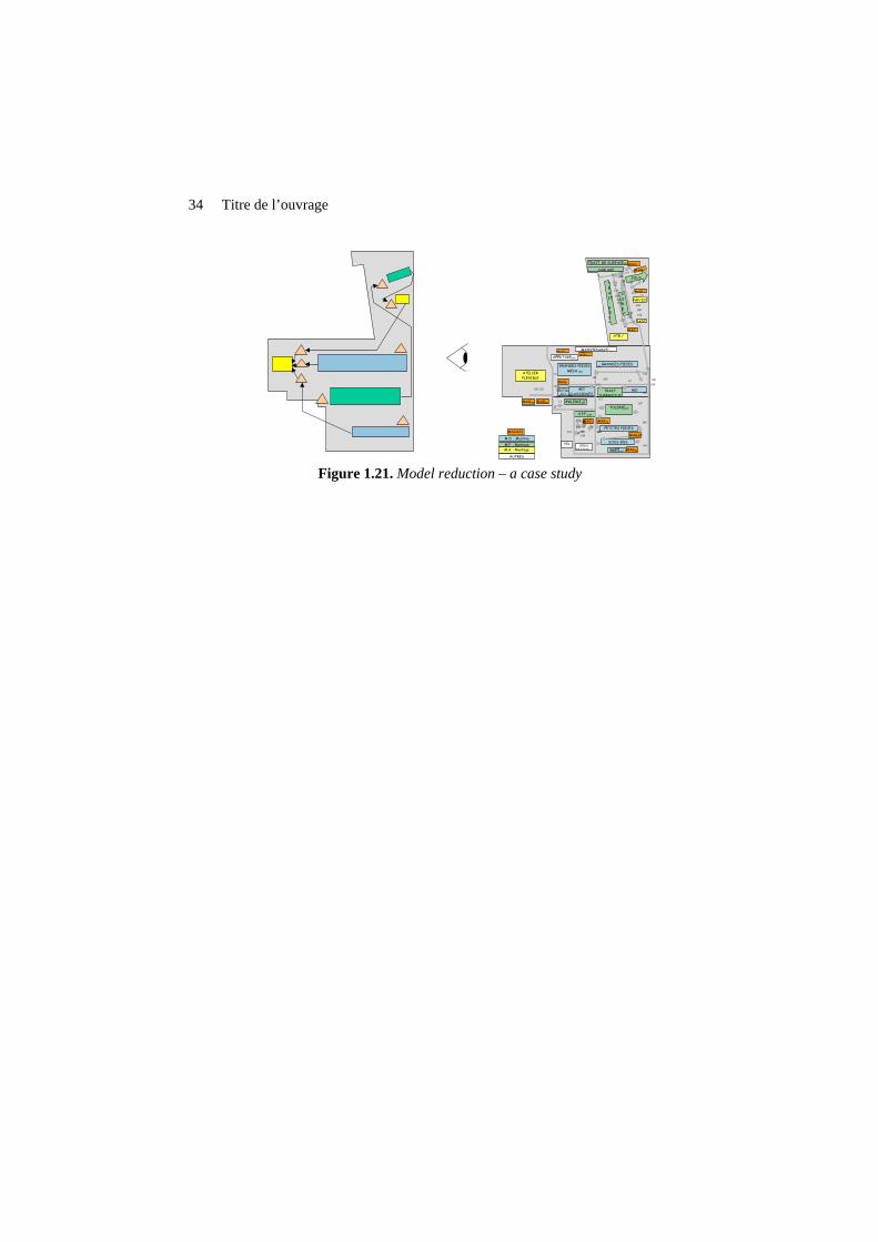
- Industrial application

This reduction method has been applied (i.e. [TEL 03]) to a factory included in an aeronautic supply chain. The model of the factory is shown on the right size of the following figure. The reduced model using this kind of method is presented on the left side of this figure. There is a strong reduction of the number of resources modelled nevertheless in a validation phase; the results of the simulation with the reduced model have been compared successfully with the real case.

Resource 4Resource 2 Resource 3

cj ti 44Resource 1 22 33

P1 =3 P3 =7 P4 =3P2 =5

p1 + p2 = 8

t j c j Resource a

p3 = 7 Resource 3

P4 = 3 Resource b


Figure 1.21. Model reduction – a case study

ATR /20

TRAIT. DE SURFACE131

TRAIT.

DE

SU

CONDUI

SABLAGE

SOUS

PAF/20

RADI

MAG1

MAG10

MAG10

ATELIERFLEXIBLE

â

MAG1

M.F. : MontageM.A. : Montage

A bl

M.O. : Machine

MAGASI

AUTRES

TOLERIE110

S.P.F.235

TOLERIE110

PETITES PIECES

SOUS-ENS

AXES185

MAGT2MAG1

MAG10

MAG10

SOUSTRAITAN

Pôlerécepti

ATELIERFLEXIBLE

OUTILLAGES204

MOCLASSIQUES

MOTRAIT.THERMIQUE1

GRANDES PIECESMECA 190

GRANDES PIECES

MAGT3MAGT4

MAGT

MAG10P MAG10

MAINTENANCE -

AFFUTAGE092

MAG10

13013

132

127105

183 122

113124125149157

163166

175190191194

197198199

101 128

102

117118

103104

106

107

108

126

11211513137

12

135

111

110

109 12184180

131

121

133

181129

14

150 13144141140

160155154

167165164

15152

161

158

169153159

201

200

156136

147146

142

182200

162


Conclusion

In this introduction chapter we have presented the main concepts which are used in supply chain management simulation. The specificities of this kind of simulation and the modelling problem difficulties in this context have been highlighted. Different types of approaches and model as been presented to solve this problem. At last, the links between the distribution level of both the system and the model have been characterised.

The following of the book includes three mains parts. The first part takes the viewpoint of the simulation model types:

- continuous simulation (chapter 2) - event system - event driven or time bucket driven (chapter 3) - simulation games (chapter 4)

The second part takes the viewpoint of the distribution level of the system and the model:

- Centralized approaches (chapter 5). - Of the interest of agents for supply chain simulation (chapter 6). - Decisional system simulation of enterprise network with MAS (chapter 7). - Simulation for Product Driven Systems (chapter 8). - HLA distributed simulation approaches for supply chain (chapter 9).

Then a third part is dedicated to the simulation products (chapter 10). Even if we are convinced of the importance of the simulation methodology, no

part of this book is explicitly dedicated to this aspect. Nevertheless the simulation methodologies (reduction simulation models, the simulation model validation and the simulation analysis) will be evocated throughout the different chapters:

- a presentation of such simulation concepts and techniques highlighted in the chapter 1,

- applications of these concepts and techniques in case studies that illustrate the pivotal role of simulation in decision-making process.


Bibliographie

[BRO 00] R. J. Brooks and A. M. Tobias – « Simplification in the simulation of manufacturing systems » - IJPR Vol38 – Pg 1009-1027 – 2000. [CHR 92] Christopher, M. L., Logistics and Supply Chain Management, London: PitmanPublishing, 1992. [COR 89] Corbier, F. (1989). Modelisation et emulation de la partie opérative pour recette en plateforme d’équipement automatisés. Thèse de doctorat, Université de Nancy I. [DEB 02] Deb K., Pratap A., Agarwal S. and Meyarivan T., A fast and elitist multiobjective genetic algorithm: NSGA-II. IEEE Transactions on Evolutionary Computation (2002), Vol. 6, pp. 182-197. [DIL 91] Dilts DM., Boyd NP., Whorms HH., The evolution of Control Architectures for automated manufacturing systems, Journal of Manufacturing systems, 1(10), 79-93,1991. [FRA 95] Frantz F.K. “A Taxonomy of Model. Abstraction Techniques”, Proceedings of the 1995. Winter Simulation Conference Washington DC Dec 95 [FUS 83] Fusaoka, A., Seki, H., Takahashi, K., 1983. A description and reasoning of plant controllers in temporal logic. In: International Joint Conference on Artiflcial Intelligence. pp. 405–408. [HUN 99] Y.F. Hung and R.C. Leachman – « Reduced simulation models of wafer fabrication facilities » - IJPR Vol37 – Pg 2685-2701 – 1999. [INN 83] G.S.Innis and E.Rexstad – « Simulation model simplification techniques » - Simulation, N°41 – Pg 7-15 – 1983. [KLE 05] Jack P.C. Kleijnen “Supply chain simulation tools and techniques: a survey ». International Journal of Simulation & Process Modelling, 1, nos 1/2, 2005, pp. 82-89. [LAW 91] A. M. Law and W. D. Kelton, (1991), Simulation Modeling & Analysis, McGraw-Hill, 2e edition. [MEN 01] Mentzer J.T., Dewitt W., Keebler J.S., Min S., Nix N.W., Smith C.D., Zacharia Z.G., Journal of business logistics Management, vol 22 n°2, 2001. [MER, 1987] C. Mercé, “Cohérence des décisions en planification hiérarchisée”. Thèse de Doctorat d’Etat, Université Paul Sabatier, Toulouse. [PAR 96] Parunak, H.V.D. (1996) ‘Applications of distributed artificial intelligence in industry’, in O'Hare, G. and Jennings, N. (Eds), Foundations of Distributed Artificial Intelligence, John Wiley & Sons. [PAR 98] Parunak, H.V.D. (1998) ‘What Can Agents Do in Industry, and Why? An Overview of Industrially-Oriented R&D at CEC’, Proceedings of the Second International Workshop on


Cooperative Information Agents II, Learning, Mobility and Electronic Commerce for Information Discovery on the Internet. [PFE 03] Pfeiffer, A., Kádár, B., Monostori, L., 2003. Evaluating and improving production control systems by using emulation. In: Applied Simulation and Modelling. [STA 00] H. Stadtler and C. Kilger, eds., Supply Chain Management and Advanced Planning, Springer, Berlin, 2000. [SCO 05] SCOR version 7, Supply Chain Council, 2005.

[TEL 03] O. Telle, C. Thierry, G. Bel, 2003, « Modélisation macroscopique des systèmes de production pour la simulation de la relation donneur d’ordres/fournisseur dans les chaînes logistiques » , 5e Congrès International de Génie Industriel : le génie industriel et les défis mondiaux, ville de Québec, Canada (in french). [TER 04] S. Terzi S. , S. Cavalieri, “Simulation in the supply chain context: a survey”, Computers in Industry vol 53, 3–16, 2004. [THO 05] A. Thomas and P. Charpentier – « Reducing simulation models for scheduling manufacturing facilities” - European Journal of Operation Research. – Vol161 - Février 2005 – Pg 111-125. [TSE 99] T.Y.Tseng, T.F. Ho and R.K. Li – « Mixing macro and micro flowtime estimation model : wafer fabrication » - IJPR – Vol37 – Pg 2447-2461 – 1999. [VOL 05] Vollmann TE, Berry WL, Whybark DC, Jacobs FR (2005) Manufacturing planning and control systems for supply chain management, 5th edn. McGraw-Hill, New York [WON 02] Wong C.Y., McFarlane D., Ahmad Zaharudin A., Agarwal V., « The Intelligent product Driven Supply Chain » 2002 IEEE International Conference on Systems, Man and Cybernetics. [ZEI 76] B.P. Zeigler – « Theory of modelling and simulation » - New York . Wiley – 1976. [MOR 03] Morel G., Panetto H., Zaremba M., Mayer F., « Manufacturing Enterprise control and management system engineering : paradigms and open issues », Annual Reviews in Control 27, 2003.

Supply chain management simulation: an overviewCaroline Thierry, Gérard Bel, André Thomas. Supply...

Documents

Transcript of Supply chain management simulation: an overviewCaroline Thierry, Gérard Bel, André Thomas. Supply...