Supplement of Earth Syst. Sci. Data, 12, 1973–1983, 2020https://doi.org/10.5194/essd-12-1973-2020-supplement© Author(s) 2020. This work is distributed underthe Creative Commons Attribution 4.0 License.

Supplement of

A deep learning reconstruction of mass balance series for all glaciers inthe French Alps: 1967–2015Jordi Bolibar et al.

Correspondence to: Jordi Bolibar (jordi.bolibar@univ-grenoble-alpes.fr)

The copyright of individual parts of the supplement might differ from the CC BY 4.0 License.

25

20

15

10

5

0

MB

(m.w

.e.) a

Mer de Glace

25

20

15

10

5

0

b

Argentiere

1990 2000 2010Year

40

30

20

10

0

c

Saint Sorlin

1990 2000 2010

20

15

10

5

0

d

GebroulazGLACIOCLIMANNANN CV

Figure S1. Comparison between glaciological observations from the GLACIOCLIM observatory, cross-validated MB reconstructions fromthis study (ANN CV) and fitted MB reconstructions (ANN). The cross-validated models are shown to display the out-of-sample performance.The fitted reconstructions display the actual reconstructions from the dataset, with models especially fitted for glaciers with data.

1 Comparison with independent geodetic mass balance data

All available annual glacier-wide MB data in the French Alps have been used to train the MB ANN of the present study. How-ever, some multi-annual geodetic mass balance (MB) datasets exist that can provide a means to validate the reconstruction’sbias for specific glaciers during multi-annual time intervals. This type of analysis is more limited than the cross-validationdone to annual glacier-wide MB values in Bolibar et al. (2020), as it only gives information about the bias of a sub-period ofthe reconstructions instead of the accuracy found via cross-validation. Our MB reconstructions are compared against ASTERgeodetic MB from Davaze et al. (2020) for the 2000-2015 and 2003-2012 periods (Fig. 2 and S2) and against Pléiades geodeticMB from Berthier et al. (2014) for the 2003-2012 period (Fig. S2).

For certain glaciers, the ASTER and Pléiades geodetic MB give a less negative MB than the glaciological SMB used totrain the deep learning SMB model. This fact might explain the slightly more negative trend of our reconstructions seen for the2000-2015 and 2003-2012 periods, which experienced very negative MB after the well known summer 2003 heatwave. Thisis quite surprising, since both the GLACIOCLIM glaciological MB measurements and the annual glacier-wide MB data fromRabatel et al. (2016) have been calibrated with geodetic MB from photogrammetric DEMs, which have a very high spatialresolution. For some regions (i.e. Grandes Rousses), the independent geodetic MB are well within the uncertainty range ofour model. However, large and steep glaciers in the Mont-Blanc massif and some other regions, such as Bossons, Talèfre andTour display important differences. These glaciers have very large and high altitude accumulation areas, not seen in almost

1

2.75

1.75

0.75

0.25

2003

-201

2 gl

acie

r-wid

e M

B (m

w.e

. a1 )

Argentière

2.75

1.75

0.75

0.25 Mer de Glace

2.75

1.75

0.75

0.25 Gébroulaz

2.75

1.75

0.75

0.25 Saint Sorlin

GCD20 B20 B14

2.75

1.75

0.75

0.25 Talèfre

GCD20 B20 B14

2.75

1.75

0.75

0.25 Tour

GCD20 B20 B14

2.75

1.75

0.75

0.25 Tré-la-Tête

GCD20 B20 B14

2.75

1.75

0.75

0.25 Bossons

Figure S2. Comparison between glaciological observations from the GLACIOCLIM observatory (GC), ASTER geodetic mass balancesfrom Davaze et al. (2020) (D20), the deep learning reconstructions from the present study (B20) and Pléiades geodetic mass balances fromBerthier et al. (2014) (B14).

any glacier in our training dataset. On the other hand, several small glaciers present very important differences, with ASTER-derived MB being much less negative than our reconstructions. Data for small glaciers carry very large uncertainties, often ofthe same order of magnitude as the observations themselves. On top of that, flat or dome-type glaciers with large white areaswith high reflectance present an important amount of noise, further increasing the associated uncertainty. This means that isquite hard to jump to conclusions from a direct comparison between these glaciers and our reconstructions. The differences andinfluence of geodetic MB on the calibration of MB series should be properly studied, as they are often not taken into accountas an additional uncertainty source. This topic goes beyond the scope of this study, but glacier modelling studies could benefitfrom integrating this in the list of uncertainties.

2 Model differences between the updated version of Marzeion et al. (2015) and this study

In order to contrast the results from Sect. 3.4, three important different aspects between our approach and the one of M15U

need to be highlighted:

1. M15U ’s model works with simplified physics, with a temperature-index model calibrated on observations; in this studywe used a fully statistical approach based on deep learning, where physics-based considerations only appear in thepredictor selection.

2. M15U calibrated their model with global MB observations, including 38 glaciers in the European Alps, most of themlocated in Switzerland for the 1901-2013 period; in this study we used observations of 32 glaciers, all located in theFrench Alps for the 1967-2015 period.

3. M15U forced their updated model with CRU 6.0 (update of Harris et al., 2014), with 0.5° latitude/longitude grid cells,which has a significantly lower spatial resolution and suitability to mountain areas than the SAFRAN reanalysis (Durand

2

et al., 2009) used in this study, in which altitude bands and aspects are considered for each massif, and meteorologicalobservations from high-altitude stations are assimilated.

The cross-validations of both studies determined a performance with an average RMSE of 0.66 m.w.e. a−1 and an r2 of0.43 for M15U for the European Alps, and an average RMSE of 0.49 m.w.e. a−1 and an r2 of 0.79 for this study. However,due to the highly different methodologies and forcings of the two models, a direct comparison is not possible, so the followinganalysis is focused on the overall trends and sensitivities in the reconstructions and their potential sources.

3 Influence of area in glacier-wide MB signal and proof on non overfitting

Due to similarities between the averaged reconstructed glacier-wide MB and the observations during the 1984-2015 period, wedecided to include an analysis to isolate the topographical influence in the glacier-wide MB signal, in order to verify that themodel is not overfitting. Since the climate signal is the main common driver of annual variability of glacier-wide MB in theregion, one needs to find a way to isolate the topographical signal. In Fig. S3, the median reconstructed annual glacier-wideMB of the 661 glaciers in the French Alps (i.e. the annual variability, hence a proxy of the climate signal) is subtracted to themean annual values of the observations and of 4 subsets of glaciers divided by area classes. Therefore, one can observe theresidual influence of glacier area on the glacier-wide MB signal. The influence of area on glaciers with observations is quitesimilar to glaciers with areas greater than 2 km2, which is reasonable since glaciers with observations have an average of 4km2 (range: 0.3-31.8 km2 in 2003). Moreover, one can see that even for a relatively short period of 30 years, the differencesbetween the reconstructions for very small glaciers (< 0.5 km2) and observations are quite important, accounting for an averagecumulative loss of more than 5 m.w.e. As stated in Sect. 2, this does not necessarily mean that the model has fully capturedthe topographical influence in the glacier-wide MB signal in the region, but it does prove that the model is not overfitting sinceit exhibits consistent variations in MB when the topographical predictors move away from the training data. Moreover, this iscoherent with the importance attributed to topographical predictors (Bolibar et al., 2020).

The same analysis has been performed with the reconstructions from the updated version of Marzeion et al. (2015) (Fig. S4).The gradient with respect to glacier surface area appears to be similar, except for the behaviour of glaciers after 2007. Smalland middle sized glaciers (0.1 - 2 km2) switch to a positive influence, as opposite to large glaciers (> 2 km2), which transitionto a negative influence. Conversely, our results show a more continuous trend, without a change of behaviour in the last yearsof the analysed period.

3

4 Supplementary figures

1985 1990 1995 2000 2005 2010 2015Year

0.2

0.0

0.2

0.4

0.6

Area

influ

ence

on

glac

ier-w

ide

SMB

sign

al (m

.w.e

. a1 )

Observations (n = 32)Glaciers < 0.1 km2 (n = 321)Glaciers 0.1 - 0.5 km2 (n = 202)Glaciers 0.5 - 2 km2 (n = 104)Glaciers > 2 km2 (n = 34)

1985 1990 1995 2000 2005 2010 2015Year

2

1

0

1

2

3

Cum

ulat

ive

area

influ

ence

on

glac

ier-w

ide

SMB

sign

al (m

.w.e

.)

Figure S3. Influence of glacier area on the glacier-wide MB signal. The reconstructed median annual glacier-wide MB of the 661 glaciers inthe French Alps can be seen as a proxy of the climate signal in the region. It is subtracted to the mean annual glacier-wide MB of the glacierswith observations and to four different subsets of reconstructions divided into glacier area size, showing only the annual differences basedon glacier area classes. The dotted line depicts the subtracted signal (non cumulative) in order to give some context.

4

1985 1990 1995 2000 2005 2010 2015Year

6

4

2

0

2

Cum

ulat

ive

area

influ

ence

on

glac

ier-w

ide

SMB

sign

al (m

.w.e

.)

ObservationsB: Reconstructed SMBB: Glaciers < 0.1 km2

B: Glaciers 0.1 - 0.5 km2

B: Glaciers 0.5 - 2 km2

B: Glaciers > 2 km2

M: Reconstructed SMBM: Glaciers < 0.1 km2

M: Glaciers 0.1 - 0.5 km2

M: Glaciers 0.5 - 2 km2

M: Glaciers > 2 km2

Figure S4. Same as S3 but comparing this study to the updated version of Marzeion et al. (2015). In the legend, “B” stands for Bolibar et al.(this study) and “M” for the update of Marzeion et al. (2015). Both models show a relatively similar gradient effect with respect to glacierarea, with differences in the amplitude of the effects. The main differences appear from 2007, where small and middle sized glaciers (0.1 -2 km2) from the update of Marzeion et al. (2015) switch to a positive influence, as opposite to large glaciers (> 2 km2), which transitionto a negative influence. The reconstructed MB dotted lines are not cumulative and they are depicted in order to give some context of thesubtracted climate signal.

5

Figure S5. Cross-validation for annual glacier-wide MB values outside the main 1984-2014 training period. The black line indicates theone-to-one reference. Simulations have been done from 1959, the earliest date with observations to validate against the maximum number ofvalues. This serves to confirm that the model is capable of reproducing glacier-wide MB outside the main observed period.

6

10 2 10 1 100 101

Surface area (km2)

1.4

1.2

1.0

0.8

0.6

0.4

0.2

0.0

Annual g

laci

er-

wid

e S

MB (

m.w

.e.a

1)

0 20 40Lowermost 20% altitudinal range slope (°)

2500 2750 3000 3250Mean altitude (m.a.s.l.)

p = 0.541

r = 0.02

p = 8.44 10-27

r = 0.42

p = 0.758

r = -0.012

Figure S6. Average annual glacier-wide MB for each glacier over the entire study period with respect to (a) glacier surface area, (b) thelowermost 20% altitudinal range slope and (c) mean glacier altitude. p indicates the p-value and r the correlation between the topographicalvariables and the average glacier-wide MB.

7

1970 1980 1990 2000 2010 2015Year

1.25

1.00

0.75

0.50

0.25

0.00

0.25

Aver

age

glac

ier-w

ide

SMB

(m.w

.e. a

1 )

Decadal average SMB (this study)Decadal average SMB (update of Marzeion et al., 2015)

Figure S7. Comparison of area-weighted decadal glacier-wide MB simulations in the French Alps between this study and an update fromMarzeion et al. (2015).

1970 1980 1990 2000 2010Year

2.5

2.0

1.5

1.0

0.5

0.0

0.5

1.0

Gla

cier

-wid

e SM

B (m

.w.e

. a1 )

Glaciers < 0.1 km2

Glaciers 0.1 - 0.5 km2

Glaciers 0.5 - 2 km2

Glaciers > 2 km2

1970 1980 1990 2000 2010Year

40

35

30

25

20

15

10

5

0

Cum

ulat

ive

glac

ier-w

ide

SMB

(m.w

.e.)

Glaciers < 0.1 km2 (n = 321)

Glaciers 0.1 - 0.5 km2 (n = 202)

Glaciers 0.5 - 2 km2 (n = 104)

Glaciers > 2 km2 (n = 34)

Figure S8. Average annual glacier-wide MB per glacier area classes

8

1970 1980 1990 2000 2010Year

2.5

2.0

1.5

1.0

0.5

0.0

0.5

Gla

cier

-wid

e SM

B (m

.w.e

. a1 )

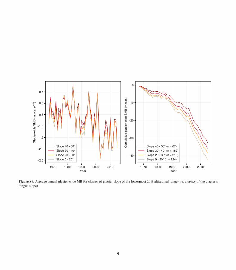
Slope 40 - 50°Slope 30 - 40°Slope 20 - 30°Slope 0 - 20°

1970 1980 1990 2000 2010Year

40

30

20

10

0

Cum

ulat

ive

glac

ier-w

ide

SMB

(m.w

.e.)

Slope 40 - 50° (n = 67)Slope 30 - 40° (n = 152)Slope 20 - 30° (n = 218)Slope 0 - 20° (n = 224)

Figure S9. Average annual glacier-wide MB for classes of glacier slope of the lowermost 20% altitudinal range (i.e. a proxy of the glacier’stongue slope)

9

Training dataset glaciersFrench Alpine glaciersRivers

Grenoble

ChamonixSPAIN

FRANCE

ITALY

Chambéry

SWITZERLAND

Gap

GERMANY

VANOISE

ECRINS

MONT

BLANC

Figure S10. French Alpine glaciers used for model training and validation and their classification into three clusters or regions (Écrins,Vanoise, Mont-Blanc). Coordinates of bottom left map corner: 44º32’ N, 5º40’ E. Coordinates of the top right map corner: 46º08’ N, 7º17’E.

10

References

Berthier, E., Vincent, C., Magnusson, E., Gunnlaugsson, A. T., Pitte, P., Le Meur, E., Masiokas, M., Ruiz, L., Palsson, F., Belart, J. M. C., andWagnon, P.: Glacier topography and elevation changes derived from Pléiades sub-meter stereo images, The Cryosphere, 8, 2275–2291,https://doi.org/10.5194/tc-8-2275-2014, https://www.the-cryosphere.net/8/2275/2014/, 2014.

Bolibar, J., Rabatel, A., Gouttevin, I., Galiez, C., Condom, T., and Sauquet, E.: Deep learning applied to glacier evolution modelling, TheCryosphere, 14, 565–584, https://doi.org/10.5194/tc-14-565-2020, https://www.the-cryosphere.net/14/565/2020/, 2020.

Davaze, L., Rabatel, A., Dufour, A., Arnaud, Y., and Hugonnet, R.: Region-wide annual glacier surface mass balance for the European Alpsfrom 2000 to 2016, Frontiers in Earth Science, 8, 149, publisher: Frontiers, 2020.

Durand, Y., Laternser, M., Giraud, G., Etchevers, P., Lesaffre, B., and Mérindol, L.: Reanalysis of 44 Yr of Climate in the FrenchAlps (1958–2002): Methodology, Model Validation, Climatology, and Trends for Air Temperature and Precipitation, Journal of Ap-plied Meteorology and Climatology, 48, 429–449, https://doi.org/10.1175/2008JAMC1808.1, http://journals.ametsoc.org/doi/abs/10.1175/2008JAMC1808.1, 2009.

Harris, I., Jones, P., Osborn, T., and Lister, D.: Updated high-resolution grids of monthly climatic observations - the CRU TS3.10 Dataset:UPDATED HIGH-RESOLUTION GRIDS OF MONTHLY CLIMATIC OBSERVATIONS, International Journal of Climatology, 34, 623–642, https://doi.org/10.1002/joc.3711, http://doi.wiley.com/10.1002/joc.3711, 2014.

11