Supervised Learning in Physical Networks: From Machine ...
18
Supervised Learning in Physical Networks: From Machine Learning to Learning Machines Menachem Stern , 1 Daniel Hexner, 2 Jason W. Rocks, 3 and Andrea J. Liu 1 1 Department of Physics and Astronomy, University of Pennsylvania, Philadelphia, Pennsylvania 19104, USA 2 Department of Mechanical Engineering, Technion, Haifa, 32000, Israel 3 Department of Physics, Boston University, Boston, Massachusetts 02139, USA (Received 10 November 2020; revised 2 April 2021; accepted 5 April 2021; published 28 May 2021) Materials and machines are often designed with particular goals in mind, so that they exhibit desired responses to given forces or constraints. Here we explore an alternative approach, namely physical coupled learning. In this paradigm, the system is not initially designed to accomplish a task, but physically adapts to applied forces to develop the ability to perform the task. Crucially, we require coupled learning to be facilitated by physically plausible learning rules, meaning that learning requires only local responses and no explicit information about the desired functionality. We show that such local learning rules can be derived for any physical network, whether in equilibrium or in steady state, with specific focus on two particular systems, namely disordered flow networks and elastic networks. By applying and adapting advances of statistical learning theory to the physical world, we demonstrate the plausibility of new classes of smart metamaterials capable of adapting to users’ needs in situ. DOI: 10.1103/PhysRevX.11.021045 Subject Areas: Metamaterials, Soft Matter, Statistical Physics I. INTRODUCTION Engineered materials are typically designed to have particular sets of properties or functions [1]. The design process often involves numerous trial and error iterations, during which the system is repeatedly tested for the desired functionality [2], modified, and tested again. Alternatively, rational design processes start from detailed knowledge of material components and typically use computation to predict the consequences of tweaking the system to sift through many possibilities. A second class of strategies is based on learning, where systems can adjust or be adjusted at the microscopic scale, in response to training examples, to develop the desired functionality. Until recently, learning strategies were pri- marily restricted to nonphysical networks such as neural networks on a computer. One class of methods, which we refer to as “global supervised learning, ” is ubiquitous for problems such as data classification [3,4]. These methods are based on the optimization of a cost or loss function that is “global” in that it depends on all of the microscopic details of the system. In the context of neural networks, for example, global supervised learning optimizes the network by modifying a set of learning degrees of freedom (e.g., weights) controlling the signal propagation between the input and output sections of the network. Global supervised learning was recently used to design flow and elastic networks—actual physical systems—with particular desired functions, e.g., allostery [5,6]. In this physical context, such learning methods were dubbed “tuning, ” since modifying the learning degrees of freedom (e.g., pipe conductances or spring constants in flow or mechanical networks, respectively) requires external inter- vention at the microscopic level. In contrast, natural systems such as the brain evolve to obtain desired functions using a fundamentally different framework of learning, which we refer to as “local learning. ” Crucially, this evolution is entirely autono- mous, requiring no external designer for evaluation of the current state of the system and its subsequent modification. In local learning, parts of the network can only adapt due to the local information available in their immediate vicinity (e.g., a synapse adapts in response to the activities only of the neurons directly connected to it [7]). It is particularly useful to apply this learning approach in physical networks such as flow or mechanical networks because the micro- scopic elements of such networks cannot perform compu- tations and do not encode information about the desired functionality a priori. Training physical networks for desired function, using either global or local supervised learning, involves two different sets of degrees of freedom. First, networks respond to source constraints by minimizing a scalar Published by the American Physical Society under the terms of the Creative Commons Attribution 4.0 International license. Further distribution of this work must maintain attribution to the author(s) and the published article’s title, journal citation, and DOI. PHYSICAL REVIEW X 11, 021045 (2021) 2160-3308=21=11(2)=021045(18) 021045-1 Published by the American Physical Society
Transcript of Supervised Learning in Physical Networks: From Machine ...
Supervised Learning in Physical Networks From Machine Learning to Learning Machines
Menachem Stern 1 Daniel Hexner2 Jason W Rocks3 and Andrea J Liu 1
1Department of Physics and Astronomy University of PennsylvaniaPhiladelphia Pennsylvania 19104 USA
2Department of Mechanical Engineering Technion Haifa 32000 Israel3Department of Physics Boston University Boston Massachusetts 02139 USA
(Received 10 November 2020 revised 2 April 2021 accepted 5 April 2021 published 28 May 2021)
Materials and machines are often designed with particular goals in mind so that they exhibit desiredresponses to given forces or constraints Here we explore an alternative approach namely physical coupledlearning In this paradigm the system is not initially designed to accomplish a task but physically adapts toapplied forces to develop the ability to perform the task Crucially we require coupled learning to befacilitated by physically plausible learning rules meaning that learning requires only local responses andno explicit information about the desired functionality We show that such local learning rules can bederived for any physical network whether in equilibrium or in steady state with specific focus on twoparticular systems namely disordered flow networks and elastic networks By applying and adaptingadvances of statistical learning theory to the physical world we demonstrate the plausibility of new classesof smart metamaterials capable of adapting to usersrsquo needs in situ
DOI 101103PhysRevX11021045 Subject Areas Metamaterials Soft MatterStatistical Physics
I INTRODUCTION
Engineered materials are typically designed to haveparticular sets of properties or functions [1] The designprocess often involves numerous trial and error iterationsduring which the system is repeatedly tested for the desiredfunctionality [2] modified and tested again Alternativelyrational design processes start from detailed knowledge ofmaterial components and typically use computation topredict the consequences of tweaking the system to siftthrough many possibilitiesA second class of strategies is based on learning where
systems can adjust or be adjusted at the microscopic scalein response to training examples to develop the desiredfunctionality Until recently learning strategies were pri-marily restricted to nonphysical networks such as neuralnetworks on a computer One class of methods which werefer to as ldquoglobal supervised learningrdquo is ubiquitous forproblems such as data classification [34] These methodsare based on the optimization of a cost or loss function thatis ldquoglobalrdquo in that it depends on all of the microscopicdetails of the system In the context of neural networks forexample global supervised learning optimizes the network
by modifying a set of learning degrees of freedom (egweights) controlling the signal propagation between theinput and output sections of the networkGlobal supervised learning was recently used to design
flow and elastic networksmdashactual physical systemsmdashwithparticular desired functions eg allostery [56] In thisphysical context such learning methods were dubbedldquotuningrdquo since modifying the learning degrees of freedom(eg pipe conductances or spring constants in flow ormechanical networks respectively) requires external inter-vention at the microscopic levelIn contrast natural systems such as the brain evolve
to obtain desired functions using a fundamentallydifferent framework of learning which we refer to asldquolocal learningrdquo Crucially this evolution is entirely autono-mous requiring no external designer for evaluation of thecurrent state of the system and its subsequent modificationIn local learning parts of the network can only adapt due tothe local information available in their immediate vicinity(eg a synapse adapts in response to the activities only ofthe neurons directly connected to it [7]) It is particularlyuseful to apply this learning approach in physical networkssuch as flow or mechanical networks because the micro-scopic elements of such networks cannot perform compu-tations and do not encode information about the desiredfunctionality a prioriTraining physical networks for desired function
using either global or local supervised learning involvestwo different sets of degrees of freedom First networksrespond to source constraints by minimizing a scalar
Published by the American Physical Society under the terms ofthe Creative Commons Attribution 40 International licenseFurther distribution of this work must maintain attribution tothe author(s) and the published articlersquos title journal citationand DOI
PHYSICAL REVIEW X 11 021045 (2021)
2160-3308=21=11(2)=021045(18) 021045-1 Published by the American Physical Society
function with respect to their physical degrees of freedomFor example central-force spring networks minimize theelastic energy by adjusting the positions of their nodes toachieve force balance on every node while flow networksminimize the power dissipation by adjusting the currents onedges to obey Kirchhoffrsquos law at every node Secondnetworks can learn specific desired target responses tosources by adjusting their learning degrees of freedomThese degrees of freedom could correspond to the stiff-nesses or equilibrium lengths of springs in a mechanicalnetwork or the conductances of edges in a flow network Inglobal supervised learning these degrees of freedom areadjusted to optimize the cost functionWe consider the case where the desired outcome of
the learning process is to achieve tailored responses ofldquotargetrdquo edges or nodes to external constraints appliedat ldquosourcerdquo edges or nodes For example an allostericresponse in a mechanical network corresponds to a desiredstrain at a set of target edges in response to a strain appliedat source edges Similarly for the simplest ldquoflow allostericrdquoresponse a pressure drop across a source edge in a flownetwork leads to a desired pressure drop across a targetedge elsewhere in the network [8]Recently it was shown that a local supervised learning
process of ldquodirected agingrdquo in which the time evolution of adisordered system is driven by applied stresses can be usedto create mechanical metamaterials with desired propertiesor functions [9ndash11] For example Refs [1011] consider aform of directed aging for a mechanical spring network inwhich the learning degrees of freedom are the equilibriumlengths of the springs comprising the network edges Theequilibrium length of each spring lengthens (shortens) if thespring is placed under extension (compression)mdashthis is alocal response to local extension (compression) Isotropiccompression [910] or repeated cycles of isotropic com-pression and expansion can drive the Poissonrsquos ratio of sucha network from positive to negative values while cycles ofcompression or stretching oscillations of source and targetedges can lead to allosteric response [11]Similarly local rules in growing vascular networks [12]
and folding sheets [1314] allow those systems to learnproperties or functions autonomously The great advantageof local supervised learning such as directed aging overglobal supervised learning is that the process is scalablemdashitcan be applied to train large systems without having tomanually modify their parts [9] In addition directed agingdoes not require detailed knowledge of microscopic inter-actions or the ability to manipulate (microscopic) learningdegrees of freedom [9]While directed aging methods are successful in training
certain physical networks for desired functions theyfail in others particularly in highly overconstrained net-works such as flow networks and high-coordinationmechanical networks Failure occurs because directedaging minimizes the physical cost function of a desired
state of the network rather than the cost function whoseminimization corresponds directly to the desired functionin global supervised learningHere we propose a general framework which we call
ldquocoupled local supervised learningrdquo for physical networkssuch as flow or mechanical networks The rules aredesigned to adjust learning degrees of freedom in responseto local conditions such as the tension on a spring in amechanical network or the current through a pipe of a flownetwork The framework provides a way of deriving rulesthat lead to modifications of learning degrees of freedomthat are extremely similar to those obtained by minimizingthe cost function As a result they are as likely to succeedin obtaining the desired response as global supervisedlearning would beThe coupled learning framework is inspired by advances
in neuroscience and computer science [15ndash19] known asldquocontrastive Hebbian learningrdquo As in contrastive Hebbianlearning one considers the response in two steady statesof the system one in which only source constraints areapplied (free state) the other where source and targetconstraints are applied simultaneously (clamped state)The particular rules we introduce which we call ldquocoupledlearning rulesrdquo are also inspired by the strategy ofldquoequilibrium propagationrdquo [18] which promotes infini-tesimal nudging and hence close proximity between thefree and clamped states In Sec II we first show in detailhow coupled learning works for flow networks (Sec II A)We successfully train such networks to obtain complexfunctionalities We then discuss the general framework ofcoupled learning in generic physical networks (Sec II B)and apply these ideas to nonlinear elastic networks(Sec II C) We demonstrate our learning framework ona standard classification problem distinguishing hand-written digits (Sec II D)It is important to note that implementation of coupled
learning should be possible in real systems In Sec IIIwe therefore consider complications that may arise inrealistic learning scenarios We first derive an approximateversion of the local learning rule that may be more easilyimplemented experimentally in a flow network (Sec III A)While inferior to the full learning rule approximatecoupled learning still gives rise to desired functionalityWe then discuss limitations due to noisy measurements ofthe physical degrees of freedom that limit the usefulness ofsmall nudging and the implications of drifting in thelearning degrees of freedom (Sec III B) Finally weaddress the effect of network size on the physical relaxationtime and the coupled learning rules (Sec III C)Following the introduction of the coupled learning rules
in Sec IV we compare coupled learning to standard globalsupervised learning frameworks that minimize a costfunction [562021] discussing the experimental realiz-ability of coupled learning in contrast with such methodsWe hope this work will stimulate further interest in
STERN HEXNER ROCKS and LIU PHYS REV X 11 021045 (2021)
021045-2
physically inspired learning opening possibilities for newclasses of metamaterials and machines able to autono-mously evolve and adapt in desired ways due to externalinfluences
II COUPLED LEARNING FRAMEWORK
A Coupled learning in flow networks
We first discuss coupled learning in the context of flownetworks Previously such networks were trained to exhibitthe particular function of flow allostery [56] using globalsupervised learning by minimizing a global cost functionSpecifically the networks were trained to have a desiredpressure drop across a target edge (or many target edges) inresponse to a pressure drop applied across a source edgeelsewhere in the network Here we show how a strictly locallearning rule can similarly train flow networksA flow network is defined by a set of N nodes labeled μ
each carrying a pressure value pμ these pressures are thephysical degrees of freedom of the network The nodes areconnected by pipes j characterized by their conductanceskj these conductances are the learning degrees of freedombecause modifying the pipe conductances will enable thenetwork to develop the desired function Assuming eachpipe is directed from one node μ1 to the other μ2 the flowcurrent in the pipe is given by Ij frac14 kjethpμ1 minus pμ2THORNequiv kjΔpjIf boundary conditions are applied to the network (egfixed pressure values at some nodes) the network finds aflow steady state in which the total dissipated power
P frac14 1
2
Xj
kjΔp2j eth1THORN
is minimized by varying the pressures at uncon-strained nodesWe now define a task for the network to learn as follows
We subdivide the physical degrees of freedom (nodepressures) fpμg into three types corresponding to source
nodes pS target nodes pT and the remaining ldquohiddenrdquonodes pH The desired task is defined such that the targetnode pressure values reach a set of desired values fPTgwhen the source node pressures are constrained to thevalues fPSg A generic disordered flow network does notpossess this function so design strategies are needed toidentify appropriate values for the pipe conductance valuesfkjg that achieve the desired taskFor the network to learn or adapt autonomously to
source pressure constraints we allow the learning degreesof freedom fkjg (pipe conductances) to vary depending onthe physical state of the network fpμg A learning rule is anequation of motion for the learning degrees of freedomtaking the form
_kj frac14 fethpμ kjTHORN eth2THORN
We focus on local learning rules where the learningdegree of freedom kj in each pipe j can only change inresponse to the physical variables (pressure values) fpμg onthe two nodes associated with pipe j pμethjTHORNWe now introduce the framework of coupled learning
Let us define two sets of constraints on the pressure valuesof the network The free state pF
μ is defined as the statewhere only the source nodes pS are constrained to theirvalues PS allowing pT pH to obtain their steady state [ieto reach values that minimize the physical cost function thedissipated power Pethpμ kjTHORN] [Fig 1(a)] The clamped statepCμ is the state where both the source and target node
pressures pS pT are constrained to PS and pCT respectively
so that only the remaining (hidden) nodes pH are allowed tochange to minimize the dissipated power The values of thedissipated power in the resulting steady states are denotedPFethPS pF
T pFH kjTHORN and PCethPS pC
T pCH kjTHORN for the free and
clamped states respectively In the following we simplifynotation by suppressing the variables in the parentheses
FIG 1 Coupled learning in flow networks (a) In the free phase node pressures are constrained such that source nodes (red) havespecific pressure values pS The target node pressures pT and the dissipated power at all pipes Pj attain their steady-state values due tothe natural flow processes in the network (b) In the clamped phase a supervisor constrains the target node pressures so that they areslightly closer to their desired values compared to the free state (c) A strictly local learning rule ie the modification of pipeconductance according to its response is proportional to the difference in dissipated power between the free and clamped states Thelearning rule thus couples the pressures at the source and target nodes
SUPERVISED LEARNING IN PHYSICAL NETWORKS FROM hellip PHYS REV X 11 021045 (2021)
021045-3
A disordered flow network constrained only at itssources (free state) will generally find a steady state inwhich the target pressures fpF
Tg differ significantly fromthe desired responses fPTg To concretely define theclamped state we introduce a trainer (supervisor) thatreads the free-state target node pressures and nudges themslightly away from their free-state pF
T values by clampingthem at
pCT frac14 pF
T thorn ηfrac12PT minus pFT eth3THORN
where η ≪ 1 [Fig 1(b)] The supervisor imposes pressureson the target nodes that are a small step closer to the desiredresponse PT We then propose a learning rule for the pipeconductance values [Fig 1(c)]
_kj frac14 αηminus1partpartkj fP
F minus PCg
frac14 1
2αηminus1ffrac12ΔpF
j 2 minus frac12ΔpCj 2g eth4THORN
where α is a scalar learning rate Note that the derivative ofthe physically minimized function (power dissipation P) istaken only directly with respect to the learning degrees offreedom fkjg (pipe conductances) excluding derivatives ofthe physical variables with respect to them (eg partpi=partkj)In the limit of small nudges η rarr 0 such derivatives cancelout when the difference between the free and clampedterms is taken [18]We note that the learning rule of Eq (4) is similar to the
one derived for analog resistor networks by Kendall et al[22] While their equation has the same form theirdefinition of the clamped state is different as they drawcurrents into the output nodes rather than fixing the outputpressures Their nudging is thus akin to applying a force onthe output nodes The simplest implementation of thelearning rule is to iteratively apply Eq (4) for some periodof time between each nudge of the clamped boundarycondition in Eq (3) Here we focus on learning in thequasistatic limit where we completely relax the nodepressure values to their steady state at each iteration toreach the minimum of the power dissipation PThe learning rule of Eq (4) is manifestly local as the
conductance of a pipe kj changes only due to the flowthrough that pipe Such local learning rules may conceiv-ably be implemented in physical pipes for which theconductance (radius) of the pipe is controlled by the currentin it Note that the network is not required to encodeinformation about the desired state function a priori Thatinformation is fed into the network by the actions of theexternal supervisor which slightly nudges the target nodepressures toward the desired state at every iteration Welater show how these properties of coupled learning stand incontrast to tuning algorithms based on optimization ofglobal cost functions
The intuition underlying coupled learning is straightfor-ward We wish to obtain a network with the desired targetpressures fPTg when source pressures fPSg are appliedWe divide the training process into small steps each ofwhich depends on free and clamped states At everyiteration of Eq (3) the clamped state is initially slightlyldquobetterrdquo than the free state in that the node pressures at thetargets fpTg are slightly closer to the desired pressuresfPTg due to the applied nudge The learning rule changesthe pipe conductances fkjg by adding the gradient at thefree state (raising the free-state power dissipation) andsubtracting the gradient at the clamped state (lowering theclamped-state power dissipation) By adjusting the pipeconductances the network response adapts to more closelyreflect the clamped state After many iterations of thelearning rule in Eq (4) f_kjg approach zero and the freestate approaches the desired target pressures PT Byiterating in this fashion the network carves out a valleyin the landscape of the dissipated power P with respect tothe target node pressures fpTg that deepens as oneapproaches the desired target pressuresmdashmuch as directedaging does when it is successful [11] This intuition impliesthat the nudge magnitude value should be small η ≪ 1 aswas proposed for equilibrium propagation [18] (see theAppendix A) Such choice allows the gradual modificationof the power landscape P so that it becomes minimal alonga valley at the desired state The approach of using smallnudges has been shown to achieve excellent results on hardcomputational learning problems such as CIFAR-10 [23]We test the coupled learning rule Eq (4) on disordered
flow networks of various sizes (N frac14 64 128 256 5121024 2048) Each of these networks is initialized withpipes of uniform conductance kj frac14 1 in Fig 2(a) In eachinstance we pick MS frac14 10 nodes randomly to be thesource nodes and apply the source pressures PS indicatedby the sizes of the red dots These source pressures arethemselves chosen randomly from a Gaussian distributionN eth0 1THORN We also randomly choose MT frac14 10 differenttarget nodes and desired pressures at target nodes fPTgrandomly from a Gaussian distribution scaled by thesource pressures N eth0 02PPSTHORN their values are indi-cated by the sizes of the blue dots in Fig 2(a) The free-state pressures pF given applied source pressures PS arefirst computed by minimizing the dissipated power Tocompare the output pF
T of the network to the desiredresponse PT we use the standard error functionC frac14 1
2
PT frac12pF
T minus PT 2 Untrained networks have a largeerror and training should gradually decrease it Thenetwork achieves the function perfectly when the errorvanishesWe now consider the clamped state by nudging the target
nodes toward their desired values setting their pressures tofpC
T frac14 pFT thorn ηfrac12PT minus pF
T g with η frac14 10minus3 We minimizepower dissipation with respect to the hidden nodes pH andthen update the conductance values (learning degrees of
STERN HEXNER ROCKS and LIU PHYS REV X 11 021045 (2021)
021045-4
freedom) according to Eq (4) with a learning rate ofα frac14 5 times 10minus4 Figure 2(b) shows the change of conduct-ance of each edge at the first iteration of learning with blue(red) signifying positive (negative) conductance changes
This process constitutes one step of the training process atthe end of each step we compute the error function C[Fig 2(d)] The difference between the obtained targets andthe desired ones decreases exponentially by many orders ofmagnitude during the training process reaching machineprecision This result demonstrates the success of thecoupled learning approach We see that the magnitude of
the change in the conductance vector jΔkj frac14ffiffiffiffiffiffiffiffiffiffiffiffiffiffiffiffiP
jΔk2jq
calculated for each step of the training process alsodecreases exponentially during training [blue dashed linein Fig 2(d)] This result shows that the learning process isadaptivemdashit slows down as it approaches good solutionsThe final trained network is displayed in Fig 2(c) withedge thicknesses indicating conductance The pipes of thetrained network have changed considerably compared tothe initial one shown in Fig 2(a) with some pipeseffectively removed (with conductances near zero)The results of applying the training protocol to networks
of different sizes for different initial networks and choicesof the source and target nodes and their pressure values areshown in Figs 2(e) and 2(f) where errors are rescaled bythe initial error for each network Our learning algorithm isgenerally able to train the networks to exhibit the desiredresponses successfully decreasing the initial error byorders of magnitude We find that networks of differentsize converge on good solutions at different rates with theerror at a particular chosen time t frac14 103 scaling roughly asa power law CethN tTHORN sim Nq (with power q in the range1ndash2) We note that networks of different sizes may not beequivalent as training may depend on idiosyncratic detailssuch as particular distances between sources and targets orother geometrical features We leave detailed exploration ofthe effects of network size and source-target geometry tofuture studyIt is noteworthy that flow networks are linear so that the
mapping between the sources to targets is always linearpT frac14 AethkTHORNPS (A is a MS timesMT matrix that depends on theconductance values) Networks which contain hundreds ofedges have many more conductance values than compo-nents of A so that there are far more degrees of freedomthan constraints While this argument suggests our flownetworks are overparametrized and should always succeedin learning we stress that not all linear transformations arepossible pressure values everywhere in the network areweighted averages of their neighbors (due to Kirchhoffrsquoslaw) More importantly the linear transformation islimited because all conductance values must be non-negative (see Appendix D) As a result flow networkscannot implement any desired linear mapping between theinputs and outputs and nonzero errors are expected forcertain tasks after training It was previously shown thatthe likelihood of flow networks to successfully learn a setof tasks depends on network size [6] even when trainedwith gradient descent Therefore we expect that traininglarger networks for a given task is more likely to succeed
FIG 2 Training flow networks with coupled learning (a) Anuntrained disordered flow network with uniform conductance atall pipes ki frac14 1 as indicated by uniform thicknesses of the greenedges The ten red and blue nodes correspond to the source andtarget nodes with dot sizes indicating the magnitudes of thesource pressures fPSg and desired target pressures fPTg (b) Ineach step conductance values are modified using Eq (4)according to the difference in flow between the free and clampedstates This process is applied iteratively (c) After training thenetwork conductance values indicated by the thicknesses of thegreen edges are considerably changed compared to the initialnetwork shown in (a) (d) During training of a network (N frac14 512nodes) the pressure values of the target nodes approach thedesired values as indicated by the exponentially shrinking error(black solid line) The desired target values fPTg are reachedwhen the error is small the modification of the conductance ineach time step Δk (blue dashed line) vanishes exponentially aswell (e) We train multiple networks of different sizesN frac14 64ndash2048 and find that all can be trained successfully withcoupled learning Error bars indicate the variation with initialnetwork and choice of sources and targets In all cases errorsdecay exponentially yet larger networks converge slower(f) Picking a certain time t frac14 103 we find that the error scalesup with system size as a soft power between 1 and 2
SUPERVISED LEARNING IN PHYSICAL NETWORKS FROM hellip PHYS REV X 11 021045 (2021)
021045-5
due to overparametrization at the expense of slowerconvergence ratesFurthermore while computational neural networks are
often initialized with random (eg Gaussian distributed)weights to compensate for their symmetries [2425] wefind that our disordered networks can be trained success-fully with uniform kj frac14 1 initialization Indeed our testswith initial weights of the form kj frac14 N eth1 σ2THORN with0 lt σ le 05 have yielded qualitatively similar results tothose shown in Fig 2(b) with respect to both training timeand accuracyRecently a similar set of ideas [2223] based
on equilibrium propagation was independently proposedto train electric resistor networks This approach is verysimilar to our framework The difference is thatRefs [2223] used a nudged state defined by injectingcurrents to target nodes instead of by clamping voltagesas in our approach Their method converges to gradientdescent in the limit η rarr 0 While our method does not wefind that coupled learning and gradient descent give verysimilar results in our trained networks (see Sec IV) Ourfocus in this paper is also somewhat different from theirswe showcase coupled learning in general physical net-works in which the system naturally tends to minimize aphysical cost function with respect to the physical degreesof freedom and emphasize considerations regarding theimplementation of coupled learning in experimentalphysical networks
B Coupled learning in general physical networks
We now formulate coupled learning more generally sothat it can be applied to general physical networksConsider a physical network with nodes indexed by μand edges indexed by j As in the special case describedearlier fxμg are physical degrees of freedom (eg nodepressure for a flow network) Network interactions dependon the learning degrees of freedom on the network edgesfwjg (eg pipe conductance in flow networks) We restrictourselves to the athermal case where given some initialcondition xμetht frac14 0THORN the physical degrees of freedomevolve to minimize a physical cost function E (eg thepower dissipation for a flow network) to reach a local orglobal minimum EethxμwjTHORN at xμ where both E and fxμgdepend on fwjgWe define the free state xFμ where the source variables xμ
alone are constrained to their values and xT xH equilibrate[ie minimize EethxμwjTHORN] At the clamped state xCμ bothsource and target variables xS xT are constrained so onlythe hidden variables are equilibrated An external trainer(supervisor) nudges the target nodes by a small amount ηtoward the desired values XT
xCT frac14 xFT thorn ηfrac12XT minus xFT eth5THORN
with η ≪ 1 The general form of coupled learning is then
_w frac14 αηminus1partwfEFethxS xFT THORN minus ECethxS xCT THORNg eth6THORN
where α is again the learning rate We thus find a generallearning rule similar to equilibrium propagation [18] withthe understanding that only the direct derivatives (partwE)are performed excluding the physical state derivativespartwxF partwxC which cancel out Given any physical networkwith a known physical cost function EethxμwjTHORN one canderive the relevant coupled learning rule directly fromEq (6) Coupled learning is performed iteratively until thedesired function is achieved Note that in physical net-works E can generically be partitioned as a sum over edgesE frac14 P
j Ej(xμethjTHORNwj) Each term Ej for edge j dependsonly on the physical degrees of freedom attached to the twonodes μethjTHORN that connect to edge j The learning rule ofEq (6) is thus guaranteed to be local in contrast to manydesign schemes relying on the optimization of a global costfunction Moreover the network is not required to encodeany information about the desired response This informa-tion is fed to the network by the trainer which nudges thetarget physical degrees of freedom closer to the desiredstate at every iteration of the learning process Note thatwhile our discussion so far and Fig 1 are restricted to aphysical network with binary edges (ie binary physicalinteractions) coupled learning does not assume binaryinteractions and is valid for arbitrary n-body potentials Formore information on the general coupled learning rule seeAppendix B
C Elastic networks
To demonstrate the generality of our coupled learningframework we apply it to another physical system central-force spring networks Here we have a set of N nodesembedded in d-dimensional space located at positionsfxμg The nodes are connected to their neighbors in thenetwork by linear springs each having a spring constant kjand equilibrium length lj The energy of a spring labeledj depends on the strain of that spring Ej frac14 1
2kjethrj minus ljTHORN2
where rj is the Euclidean distance between the two nodesconnected by the spring The physical cost function in thiscase is the total elastic energy of the network given byE frac14 P
jisinsprings Ej We choose source and target springswhose lengths are rS and rT and train the network so thatan application of source edge strains fRSg gives rise todesired target edge strains fRTgIn contrast to flow networks spring networks are non-
linear in the physical variables fxμg due to the nonlinearityin the Euclidean distance function Moreover while thespring constants fkjg are formally equivalent to conduc-tances in flow networks the equilibrium lengths fljg haveno direct analog in flow networks These extra variables are
STERN HEXNER ROCKS and LIU PHYS REV X 11 021045 (2021)
021045-6
additional learning degrees of freedom that we can adjust inaddition to the spring constantsThe free and clamped states of the spring network are
applied similarly to the previous example with the excep-tion that we define the source and target boundary con-ditions on the edges of the network rather than the nodesdemonstrating that the coupled learning framework can beapplied in either case Next we apply the coupled learningrule (6) to obtain two separate learning rules one for thespring constants kj the other for the rest lengths lj
_kj frac14α
η
partpartkj fE
F minus ECg
frac14 α
2ηffrac12rFj minus lj2 minus frac12rCj minus lj2g
_lj frac14α
η
partpartlj
fEF minus ECg
frac14 α
ηkjffrac12rFj minus lj minus frac12rCj minus ljg eth7THORN
Learning in elastic networks can be accomplishedthrough modification of the spring constants rest lengthsor a combination of both As before Eq (7) gives locallearning rules where each spring only changes due to thestrain on that particular spring To test these learning ruleswe train elastic networks with N frac14 512 and N frac14 1024nodes with multiple choices of 10 random source strainsand 3 random target strains Elastic network calculationswere performed using a specialized benchmarked set ofcomputational tools used earlier for research on tunednetworks [526] The success of the training is againassessed using the error C frac14 1
2
PT frac12rFT minus RT 2 measuring
deviation from the desired target lengths We find thatregardless of whether the network learns by modifying itsspring constants [Fig 3(a)] or rest lengths [Fig 3(b)] thenetworks are consistently successful in achieving the desiredtarget strain reducing the error C by orders of magnitudeLarger networks take slightly longer to learn but achievesimilar success We find that the rest-length-based learning
rule gives somewhat more consistent learning results fordifferent networks and source-target choices as evidencedby smaller error bars in Fig 3(b) Recently a rule similar tothat of Eq (7) was used to prune edges in elastic networks toobtain desired allosteric responses [27] It is notable thatRef [27] uses a ldquosymmetrizedrdquo version of the learning rulewhere the free state is replacedwith a negative clamped statewhere the output nodes are held farther away from theirrespective desired value
D Supervised classification
In Secs II A and II C we trained networks to exhibitfunctions inspired by allostery in biology obtaining adesired map between one set of sources (inputs) and oneset of targets (outputs) Here we train flow networks todisplay a function inspired by computer science namelythe ability to classify images In classification a network istrained to map between multiple sets of inputs and outputsIn order to use our coupled learning protocol for simulta-neous encoding of multiple input-output maps we slightlymodify the training process in the spirit of stochasticgradient descent [28] Each training image provides aninput and the correct answer for that image is the desiredoutput Training examples are sampled uniformly at ran-dom and the coupled learning rule of Eq (4) is appliedaccordinglyA simple example of a classification problem often used
to benchmark supervised machine learning algorithms is todistinguish between labeled images of handwritten digits(MNIST [29]) Each image corresponds to a particularinput vector (eg pixel intensity values) while the desiredoutput is an indicator of the digit displayed Typically analgorithm is trained on a set of example images (trainingset) while the goal is to optimize the classificationperformance on unseen images (test set)Here we train flow networks to distinguish between
images of two digits (0 and 1) We pick 50 images of eachdigit (class) from the MNIST database to serve as a trainingset and an additional 50 images of each digit as a test setInstead of using the images themselves we first carry out aprincipal component analysis of all MNIST images andtrain the network using the top 25 principal components ofthe training set images The inputs (source pressures) aregiven by these principal components of the training imagesfor a randomly selected set of 25 source nodes Weadditionally pick 2 random output (target) nodes one foreach digit The desired output for a training examplecorresponding to a 0 is for the first output node the 0target node to have high pressure (plsquo00 frac14 1) and for thesecond output node the 1 node to have no pressure(plsquo10 frac14 0) The target pressures are reversed when anexample corresponding to the digit 1 is chosen so thatthe 1 node has plsquo10 frac14 1 and the 0 node has plsquo00 frac14 0 At eachiteration of the learning rule the network is presented witha single training image sampled uniformly at random from
(a) (b)
FIG 3 Training spring networks by modifying (a) springconstants or (b) rest lengths The error in the target edge lengthsis shown as a function of the number of training iterations forN frac14 512 (black circles) and N frac14 1024 (blue squares) networksTraining by coupled learning is successful for either the stiffnessor rest length degrees of freedom
SUPERVISED LEARNING IN PHYSICAL NETWORKS FROM hellip PHYS REV X 11 021045 (2021)
021045-7
the training set and is nudged toward the desiredoutput for that image A training epoch is defined as thetime required for the network to be presented with 100training examplesThe error between the desired and observed behavior is
shown in Fig 4(a) for each of the digits The solid linesrepresent errors for the training set while the dashed linesshow errors for the test set We see that the network notonly reduces the training error but also successfullygeneralizes reducing the test errors as well While thepressure at the output nodes is continuous we want thenetwork to make a discrete choice about the label ofthe shown image We say that the predicted label is givenby the target node with the larger pressure With thisdefinition we see that the classification accuracy of thenetwork starts at about 50 and improves dramaticallyduring training [Fig 4(b)] After training the overalltraining accuracy reaches 98 while the test accuracy is95 This learning performance is almost as good as thatof simple machine learning algorithms such as logisticregression which for the same data yields a trainingaccuracy of 100 and a test accuracy of 98 Note that
we did not tune hyperparameters to achieve the listedaccuracies such tuning might well improve the perfor-mance of our algorithm In Figs 4(c) and 4(d) the networkresponse to two select input images is shown When thesource nodes are constrained with pressure values corre-sponding to an image of a 0 the 0 target node has highpressure (blue) while the 1 target node has very lowpressure The opposite response occurs when an imageof a 1 is applied as inputAs discussed above we used a training approach in the
spirit of stochastic gradient descent training the networkwith one training example at a time We note that it may beexperimentally possible to train the network using batchgradients presenting many training examples in quicksuccession so that the learning rule averages the conduct-ance update over these examples A similar effect can beachieved by maintaining the rate of example presentationyet slowing down the learning rate α
III EXPERIMENTAL CONSIDERATIONS
In the previous section we introduced the coupledlearning rules that respect the physical requirements oflocality and the fact that the desired response cannot beencoded in the network a priori We have demonstratedcomputationally that flow and mechanical networks suc-cessfully learn desired behaviors using such learning rulesFor networks to learn autonomously in a physical settingthe network must be able to implement the coupledlearning rules as the physical dynamics of their learningdegrees of freedom Furthermore an external supervisorneeds to be able to clamp the target nodes as needed Forfluid flow networks coupled learning requires the cou-pling of pipe conductance values to the flow inside thepipe For example constriction of pipes can be achievedby entrainment of sediment in the flow and its depositioninside the pipes [3031] These dynamics could support aone-sided learning rule as described in Sec III A In elasticnetworks either the stiffnesses or rest lengths of bondsneed to change for learning to be possible Several classesof materials are known to adapt their stiffness in responseto applied strain eg ethylene vinyl acetate [32] andthermoplastic polyurethane [33] The former has beenused to train materials for auxetic behavior using directedaging [9]In the following we describe some potential experi-
mental difficulties in implementing coupled learning inphysical networks and how they may be overcome Wefirst discuss an approximation to the coupled learningrules allowing for a simpler implementation in flownetworks (Sec III A) Then we describe the effects ofplausible experimental issues such as noisy physicaldegrees of freedom or drifting learning degrees of freedom(Sec III B) and the effect of network size on the physicalrelaxation assumed in coupled learning (Sec III C)
FIG 4 Classification of MNIST digits (0rsquos and 1rsquos) (a) Theclassification error (value of cost function) [Eq (11)] for thedigits 0 (blue) and 1 (black) versus the number epochs whereeach epoch consists of 100 iterations of the learning rule with adifferent randomly selected training image presented at eachiteration Training error is indicated by solid lines and test errorby dashed lines (b) Prediction accuracy on test images (fractionof correct predictions made by the network for digits 0 and 1)versus number of epochs Total test accuracy shown in red (c)(d)Response of the network when presented with the image at thetop left The power dissipated at each edge is indicated by theintensity of the edge color while the pressures of target nodes arelabeled with blue (0) and black (1) circles When a 0 image isshown the 0 target node has high pressure (blue circle) and the 1target node has low pressure when a 1 image is shown the 1target node has high pressure (black circle) and the 0 target nodehas low pressure
STERN HEXNER ROCKS and LIU PHYS REV X 11 021045 (2021)
021045-8
A Approximate learning rules
Consider the flow networks described earlier To imple-ment the learning rule of Eq (4) one requires pipes whoseconductance can vary in response to the dissipated flowpower through them There are two major issues inimplementing this learning rule in a physical flow networkFirst the learning rule of Eq (4) for the conductance onedge j depends not simply on the power through edge j buton the difference between the power when the free-boundary condition and the power when the clamped-boundary condition are applied This is difficult to handleexperimentally because it is impossible to apply both setsof boundary conditions simultaneously to extract thedifference One could try to get around this by alternatingbetween the free- and clamped-boundary conditions duringthe process but then one runs into the difficulty that thesign of conductance change is opposite for the two types ofboundary conditions In other words the same powerthrough edge j in the free and clamped states would needto induce the opposite change in conductance Alternatingthe sign of the change in conductance along with theboundary conditions poses considerable experimental dif-ficulty The second hurdle is that Eq (4) requires that pipesmust be able to either increase or decrease their conduct-ance Pipes whose conductance can change in only onedirection (eg decreasing k by constriction) are presum-ably easier to implement experimentallyTo circumvent these difficulties we seek an appropriate
approximation of Eq (4) (see Appendix C for more details)that is still effective as a learning rule We first define anew hybrid state of the system named the δ state inwhich the power dissipation is minimized with respectto the hidden node pressures pH with the constraintspS frac14 0 pT frac14 minusηethPT minus pF
T THORNNote that this state corresponds to constraining the
source and target nodes to the desired pressure differencesbetween the free and clamped states according to theoriginal approach Now we may expand the clamped-statepower in series around the free state to obtain a newexpression for the learning rule in terms of the δ state andfree state
_kj asymp 2αηminus1ΔpFj Δpδ
j
Ideally only the δ state would be involved in the learningrule and not the free state Let us simplify this rule by onlyaccounting for the sign of the free pressure drop sgnethΔpF
j THORNreturning 1 depending on the sign of flow in the freestate _kj asymp 2αηminus1sgnethΔpF
j THORNΔpδj
The resulting learning rule while only depending on thepressures at the δ state can still induce either positive ornegative changes in k To avoid this we may impose a stepfunction that only allows changes in one direction (egonly decreasing k)
_kj frac14 minus2αηminus1ΘethminusΔpFj Δpδ
jTHORNjΔpδjj eth8THORN
The intuition behind this learning rule is relativelysimple if for a particular pipe sgnethΔpF
j THORNΔpδj lt 0 then
too much flow is going through the pipe in the free stateThus one could improve the functional result by decreas-ing the conductance of that pipeThis learning rule may be simpler to implement physi-
cally but is it a sufficiently close approximation of theoriginal rule In Fig 5 we train a network (512 nodes with10 random sources and 3 random targets) using the learningrules of Eqs (4) and (8) In Fig 5(a) the learning rules arecompared to the tuning algorithm [Eq (13)] by taking thedot product of these modification [similar to Fig 7(c)]While the approximate learning rule has a lower dotproduct with the optimal local tuning for all values of ηcompared to the full learning rule the correlations are stillvery significant We thus expect the approximate learningrule to train the network successfully Indeed we find thatwhen the approximate learning rule is applied iterativelythe learning process is successful yielding a decrease of theerror C of at least an order of magnitude [Fig 5(b)] Whilethe approximate training typically plateaus at a higher errorlevel compared to the full coupled learning rule theapproximate learning rule can successfully train flownetworks to exhibit random source-target responses
B Noise in physical or learning degrees of freedom
So far we have assumed that coupled learning modifiesthe learning degrees of freedom given precise knowledge ofthe free and clamped states [eg PF PC in Eq (4)]However in any physical implementation of a networkthere will be errors in the measurements of these statesSuppose that measurement of the dissipated power at every
(a) (b)
FIG 5 Training a flow network (512 nodes 10 randomsources and 3 random targets) with an approximate experimen-tally viable learning rule (a) The full coupled learning rule[Eq (4)] and the approximate learning rule [Eq (8)] are comparedto the gradient of the cost function for different values of η [seeFig 7(c)] While the full learning rule is superior there is still asignificant correlation between optimal tuning and the approxi-mate rule (b) The network may be trained using both the full andapproximate rule at similar timescales The approximate learningrule being much more restricted often saturates at a higher errorlevel compared to the full rule (averaged over 17 random source-target sets)
SUPERVISED LEARNING IN PHYSICAL NETWORKS FROM hellip PHYS REV X 11 021045 (2021)
021045-9
edge is subject to additive white noise of magnitude ϵnoted ej simN eth0 ϵ2THORN The learning rule would then containan extra term due to the noise
_kj asymp1
2αηminus1ffrac12ΔpF
j 2 minus frac12ΔpCj 2 thorn ejg eth9THORN
It is clear from Eq (9) that if the error magnitudeϵ is larger than the typical difference between thefree and clamped terms the update to the conductancevalues would be random and learning will fail Aswe show in Appendix B the difference between the freeand clamped term scales with the nudge amplitudefrac12ΔpF2 minus frac12ΔpC2 sim η2 Put differently when the nudgeis small (η rarr 0) the free and clamped states are nearlyidentical so that their difference is dominated by noiseThis raises the possibility that increasing the nudgeamplitude η used ie nudging the clamped state closerto the desired state will increase the relative importance ofthe learning signal compared to the noise allowing thenetwork to learn despite the noiseTo test this idea we train a flow network of N frac14 512
nodes on a random task with 10 source and 10 target nodes[the same training problem shown in Figs 2(a)ndash2(d)]While training we inject white noise of given magnitude ϵaccording to Eq (9) As suggested we find that theseldquomeasurementrdquo errors primarily spoil learning at low nudgevalues so that increasing ηmight have a beneficial effect onlearning [Fig 6(a)] We conclude that experimental settingswith finite measurement errors induce a trade-off in thenudge parameter η Nudges should be small so that thelearning rule gives a good estimate of the desired gradientsyet they cannot be too small or the learning will bedominated by noiseAnother source of error in an experimental realization of
learning networks may be unwanted fluctuations or drift inthe learning parameters For example it is known thatnatural neural networks undergo synaptic fluctuations evenin adults and in the absence of synaptic activity [34ndash36] Insynthetic contexts engineering materials with controllable
parameters in a wide range eg variable stiffness in shapememory alloys [37] can lead to an increased volatility inthese controlled parameters [38]Drifting in the learning degrees of freedom during
the training process is expected to impede learning Tostudy its effects we assume that the learning degrees offreedom fluctuate with some magnitude δ for all edgesThis gives rise to additive white noise dj simN eth0 δ2THORN in thelearning rule
_kj asymp1
2αηminus1ffrac12ΔpF
j 2 minus frac12ΔpCj 2g thorn dj eth10THORN
In contrast to the noise in the physical degreesof freedom discussed earlier such diffusion cannot becontrolled by increasing the nudge amplitude Howeverone can increase the learning rate α to hasten the learningdynamics compared to diffusion (keeping in mind thatto maintain convergence learning cannot be made toofast [4])Once more we train a flow network (N frac14 512 nodes) on
a task with 10 random sources and 10 random targets [thesame task as in Figs 2(a)ndash2(d)] The network is trainedwith different diffusion magnitudes δ and two differentlearning rates α frac14 02 04 We find that given constantdiffusion rates training is more successful at a higherlearning rate as expected [Fig 6(b)] These results showthat unavoidable experimental issues such as noise in thephysical and learning degrees of freedom can be mitigatedby controlling learning hyperparameters such as the nudgeamplitude η and the learning rate α
C Physical relaxation
In this work we have taken the quasistatic limit ofcoupled learning so that before computing either the free orthe clamped state the network first reaches its stableequilibrium (or steady state) In other words we exploredthe limit where learning is much slower than the physicaldynamics [39] Physical networks however take finite timeto relax to their equilibrium which does not scale with theamplitude of perturbation η (in the linear response regime)Therefore using small nudges in general does not help withaccelerating the physical relaxation of the network towardits equilibrium statesMoreover the nudging between the free and clamped
states induces a local perturbation whose informationcontent must propagate to the entire network before itcan equilibrate In both flow networks and elastic springnetworks the time for this information propagation is set bythe speed of sound In flow networks the speed of sounddepends on the compressibility of the fluid Similarlyelastic spring networks have a finite speed of sounddepending on their node masses edge spring constantsand network structure This information propagation timeimplies a linear lower bound on the scaling of the relaxation
(a) (b)
FIG 6 Learning with noisy measurements and diffusinglearning degrees of freedom (a) When noise is present in thefree- or clamped-state measurements small nudges impedelearning Training results can be improved with larger η lt 1nudges (b) Drifting in the learning degrees of freedom impedeslearning but its effects can be mitigated by increasing thelearning rate α
STERN HEXNER ROCKS and LIU PHYS REV X 11 021045 (2021)
021045-10
time with system size Depending on the physics of thenetwork and its architecture relaxation time might scalemore slowly with size For example in large brancheddissipative flow networks the response time to a perturba-tion scales quadratically [40]Consider a flow or elastic network of linear dimension L
trained by waiting time τ for relaxation before updating thelearning degrees of freedom in Eq (6) Because of theaforementioned considerations training a larger network oflinear dimension L0 would require waiting τ0 asymp τfethL0=LTHORN(withf a faster than linear function) for similar relaxation sothat the overall training time should scale with the physicallength of the network Note that this physical time scaling isdifferent from the scaling of learning convergence withsystem size discussed earlier At the limit of small enoughlearning rates α when the learning dynamics effectivelyapproximate gradient descent on the cost function we arguethat rescaling the learning rate in Eq (6) by α0 frac14 αfethL0=LTHORNwould counteract this increase in training timeHowever thelearning rate cannot increasewithout bound for two reasonsFirst at high learning rates learningmay not converge as thegradient step may overshoot the minimum of the costfunction as is often the case in optimization problems[4] Furthermore increasing the learning rate compared tothe physical relaxation rate would eventually break thequasistatic assumption in Eq (6) We leave the effects ofbreaking the assumption of quasistaticity to future study
IV COMPARISON OF COUPLED LEARNING TOOTHER LEARNING APPROACHES
To emphasize the advantages of our local supervisedlearning approach we compare it to global supervisedlearning where we adjust the learning degrees of freedomto minimize a learning cost function (or error function)Such a rational tuning strategy was previously demon-strated to be highly successful [6] and is fundamental tosupervised machine learning [4] Here we compare coupledlearning and tuning in the contexts of flow and elasticnetworksOne usually defines the learning cost function as the
distance between the desired response PT and the actualtarget response pF
T A commonly chosen function is the L2
norm (Euclidean distance)
Cequiv 1
2frac12pF
T minus PT 2 eth11THORN
A straightforward way to minimize this function withrespect to the learning degrees of freedom (pipe conduct-ance values fkjg) is to perform gradient descent In eachstep of the process the source pressures fPSg are appliedthe physical cost function (total dissipated power) isminimized to obtain the pressures fpF
Tg the gradient ofthe learning cost function is computed and the conduc-tances fkjg are changed according to
partkC frac14 frac12pFT minus PT middot partkpF
T
_kG frac14 minusαpartkC eth12THORN
where _kG denotes the change in the pipe conductancepredicted by the tuning (global supervised learning) strat-egy Note that such a process cannot drive autonomousadaptation in a physical networkmdashEq (12) cannot be aphysical learning rulemdashfor two fundamental reasons Firstthe update rule is not local Generally the target pressurepFT depends on the conductance of every pipe in the
network so each component of partkC contains contributionsfrom the entire network The modification of each pipeconductance depends explicitly on the currents through allof the other pipes no matter how distant they are Secondthe tuning cost function C depends explicitly on the desiredresponse PT Thus if the network computes the gradient itmust encode information about the desired response Arandom disordered network is not expected to encode suchinformation a priori Together these two properties of thetuning process imply that this approach requires bothcomputation and the modification of pipe conductancevalues by an external designermdashit cannot qualify as aphysical autonomous learning processThe second point above that the tuning cost function
depends explicitly on the desired behavior PT deservesfurther discussion In coupled learning the desired targetvalues PT do not appear explicitly in the learning rule ofEq (4) but do appear explicitly in the definition of theclamped state [Eq (3)] This is a subtle but crucialdistinction between coupled learning and tuning Incoupled learning a trainer (supervisor) imposes boundaryconditions only on the target nodes The physics of thenetwork then propagates the effect of these boundaryconditions to every edge in the network Then each edgeindependently adjusts its learning degrees of freedomtaking into account only its own response to the appliedboundary conditions In other words the boundary con-ditions imposed by the trainer depend on the desiredresponse fPTg but the equations of motion of the pipeconductance values fkjg themselves do not require knowl-edge of fPTg once the boundary conditions are appliedThe trainer needs to know the desired network behaviorbut the network itself does not In the tuning process bycontrast the pipe conductance values evolve according toan equation of motion that depends explicitly on fPTgThus tuning a physical network requires external compu-tation of partkC and the subsequent modification of thelearning degrees of freedom by an external agentThe difference between local and global supervised
learning has fueled long-standing debates on how biologi-cal networks learn and their relation to computationaltuning approaches such as machine learning algorithms[41] While natural neural systems are complicated and canperform certain computations simple physical networks
SUPERVISED LEARNING IN PHYSICAL NETWORKS FROM hellip PHYS REV X 11 021045 (2021)
021045-11
such as the ones studied here definitely cannot In order forthese networks to adapt autonomously to external inputsand learn desired functions from them without performingcomputations we need a physically plausible learningparadigm such as the coupled learning framework pre-sented hereWe now directly compare results of the two learning
methods in flow and elastic networks First we use bothmethods to train flow networks of size N frac14 512 nodes onthe tasks described in Sec II A [Fig 7(a)] We find that onaverage coupled learning is as efficient as tuning (gradientdescent) for training these networks Indeed for theproblem shown in Fig 2(d) coupled learning actuallyconverges faster than tuningTo explore the comparison further we denote the
conductance modification prescribed by coupled learningas _kCL [Eq (4)] and the conductance modification dictatedby global supervised learning or tuning as _kG [Eqs (11)and (12)] We argue theoretically in Appendix B thatcoupled learning leads to modifications to the learningdegrees of freedom kj that are similar to those obtained bytuning using gradient descent [Eq (12)] Therefore wecompare the two modification vectors directly by taking adot product between them (after normalization)
_kCL sim partkfPF minus PCg_kG sim minuspartkC eth13THORN
These two modification vectors are compared inFigs 7(b)ndash7(d) for flow networks with N frac14 512 nodestrained with 10 random sources and varying numbers ofrandom targets Most notably we observe that the twovectors are indeed nearly identical (the dot product of thenormalized vectors is close to unity) for sufficiently smallnudges η [Fig 7(c)] This is remarkable as the vectorsreside in the very high (sim1000) dimensional space ofconductance values k of the network Thus Fig 7 showsthat the local process of coupled learning follows atrajectory in conductance space that is very similar tothe trajectory followed during rational tuning which is aglobal supervised learning process [although we do notefluctuations in the dot product see the enlarged scale inFig 7(b) and Appendix D] For small nudges η≲ 01we observe a plateau in this dot product so the precisechoice of η is not important [choosing small η rarr 0 leads toa well-defined limit of the coupled learning rule of Eq (13)see Appendix B] On the other hand choosing large η sim 1(as in Hebbian contrastive learning) leads to significantdifferences between the two processes We also note thatfor more complicated functions (more targets to satisfy)the dot product slightly decreases This effect is exhibitedin Fig 7(d) for networks of two sizes However even withextra functional complexity coupled learning yields resultsthat are remarkably similar to tuning
Unlike flow networks elastic spring networks arefundamentally nonlinear so it is interesting to explorewhether coupled learning produces similar modifications tothe learning degrees of freedom as tuning (gradientdescent) In Figs 7(e) and 7(f) we show the alignmentbetween the coupled learning and tuning We find that thealignment between these modification vectors is still verysignificant especially for training with the stiffness degreesof freedom kj We further find that the alignment is reducedduring training as the network approaches low-error sol-utions in particular for training the rest lengths lj While
(c) (d)
(e) (f)
(a) (b)Linear flow networks
Nonlinear spring networks
FIG 7 Coupled learning (local supervised learning) comparedto tuning (global supervised learning) in linear flow and nonlinearelastic networks (a) Direct comparison between training traces inflow networks shows that coupled learning is as successful asgradient descent (b) The dot product of the modification vectorΔk for coupled learning and tuning (gradient descent) duringtraining undergoes fluctuations yet remains high (c) At thebeginning of training we compute the dot product of themodification vector Δk for coupled learning and tuning as afunction of the nudge variable η for systems with 1 (red triangles)3 (blue diamonds) and 10 (black crosses) target nodes The twomethods predict very similar results for η ≪ 1 (d) For η frac14 10minus3coupled learning yields similar results to tuning for networks withN frac14 512 (black circles) and N frac14 1024 (blue squares) as afunction of the number of target nodes (e)(f) Dot productbetween the normalized predictions of coupled learning andgradient descent in nonlinear elastic networks We find thatcoupled learning and gradient descent are largely aligned duringthe training of elastic networks using the stiffness and rest lengthsdegrees of freedom (N frac14 512 1024 MS frac14 10 MT frac14 3)
STERN HEXNER ROCKS and LIU PHYS REV X 11 021045 (2021)
021045-12
this result is interesting and suggests that coupled learningmay differ significantly from tuning in certain nonlinearnetworks we note that training the network is successfulregardless of the deviation between the methods We leavemore detailed exploration of the alignment between pos-sible local learning rules to future studyA physical learning process called ldquodirected agingrdquo has
recently been introduced to create mechanical metamate-rials from mechanical networks [9ndash11] and self-foldingsheets [13] The strategy exploits the idea that stressedbonds in elastic networks tend to weaken (age) over timeDuring training the network is nudged in a similar fashionto the coupled learning process References [910] considertwo different classes of learning degrees of freedom incentral-force spring networks In one case the ldquok modelrdquothe stiffnesses kj of the springs are modified while in theldquolmodelrdquo rest lengths l0j are modified The clamped statecan correspond either to Eq (5) with η frac14 1 or to aperiodically varying amplitude η frac14 sinΩt In the lattercase the oscillation is performed quasistatically in thesense that the physical degrees of freedom are relaxedcompletely at each time stepIn elastic networks the directed aging k-model and
l-model learning rules are
_kj frac14 minusα
2frac12rCj minus lj2
_lj frac14 minusαkjfrac12rCj minus lj eth14THORN
where the learning degrees of freedom (stiffness or restlength) evolve in response to the clamped boundaryconditions Such dynamics have the effect of loweringthe elastic energy of the desired state and thus the responseof the network to the specified inputs is expected toimprove Indeed directed aging was shown to be successfulin training elastic networks with nearly marginal co-ordination so that they lie just above the minimum numberof edges per node (Zc frac14 2d) required for mechanicalstability in d dimensions Note that because the clampedphysical cost function EC can be written as a sum overindividual costs of edges j the directed aging rule is localas it is for coupled learning Directed aging thereforecorresponds to a physical learning rule as has beendemonstrated experimentally [9]However directed aging fails to achieve the desired target
response in many instances In particular it is observed thateither flow networks or highly coordinated elastic networkscannot be trained by directed aging to perform allostericfunctionsComparing directed aging [Eq (14)]with coupledlearning [Eq (7)]we see that theclamped termsare the samebut the directed aging rule is missing the free term As aspecial caseof coupled learningdirectedaging is expected toperformwell in systemswhose energy in the free state (or itsderivative) can be neglected Appendix B shows that ingeneral both the free andclamped termsare necessary to train
networks for desired functions Therefore coupled learningcan be viewed as a generalization of the directed agingframework that is successful for a more general class ofphysical networks
V DISCUSSION
In this work we have introduced coupled learning a classof learning rules born of contrastive Hebbian learning andequilibrium propagation [1518] and applied it to two typesof physical systems namely flow networks and mechanicalspring networks The advantage of such supervised learn-ing rules compared to more traditional techniques such asoptimization of a cost function is that they are physicallyplausible at least in principle coupled learning can beimplemented in realistic materials and networks allowingthem to learn autonomously from external signalsSuch learning machines are not only interesting in
themselves but may have important advantages comparedto physical systems designed by optimizing a cost functionFirst because the process involves local responses to localstresses the approach is scalablemdashtraining steps in net-works of different sizes (different numbers of nodes) wouldtake approximately the same amount of time In contrastthe time required to compute gradients of a collective costfunction increases rapidly with system sizeSecond the ability to train the system in situ means
that it is not necessary to know the network geometry ortopology or even any information about the physicalor learning degrees of freedom This is particularlyvaluable for experimental systems which do not have tobe characterized in full microscopic detail in order to betrained as long as the proper learning rules can beimplemented at least in an approximate formThird as long as the learning rules can be implemented
one does not need to manipulate individual edges tohave the desired values of the learning degree of freedom(eg theedgeconductancefora flownetwork)Thus theroleof the supervisor can be filled by an end user training thenetwork for theirdesired tasks rather thananexpert designerAn experimental realization of a learning flow network
seems quite plausible as has also been suggested for analogresistor networks [22] The required ingredients are pipeswhose conductances can be modified in response to thecurrent carried by the pipe It is possible that this conditionis similar to that used by the brain vasculature wherevessels can be expanded or constricted [4243]We have focused primarily on training physical networks
for one particular function (ie one particular source-targetmap namely allostery) However coupled learning rulesmay be used as a stochastic gradient descent step trainingthe network for a different function in each trainingiteration This idea allowed us to train the flow networkto distinguish MNIST digits The dynamics of learningmultiple functions using coupled learning is quite involvedand the training performance may depend strongly on the
SUPERVISED LEARNING IN PHYSICAL NETWORKS FROM hellip PHYS REV X 11 021045 (2021)
021045-13
order and frequency of shown training examples We willaddress these issues in subsequent workOne might ask whether physical networks could com-
pete as learning machines with computational neural net-works Our aim is not to outperform neural networksRather the goal is to design physical systems capable ofadapting autonomously to tasks and able to generalize todiverse inputs without a computer Nevertheless physicalnetworks do supply at least one potential advantagecompared to computational neural networks In contrastto feed-forward neural networks often used in machinelearning the input-output relations in our physical (recur-rent) networks are necessarily symmetric in the linearresponse regime (the regime in which the target responseis proportional to the source) As a result training targetresponses for given sources may yield a generative model[4445] Such generative models could produce examplesof a class given its label by imposing target valuesdistributed around the trained responses and reading outthe free source values We leave the prospects of physicallearning of generative models to future study
ACKNOWLEDGMENTS
We thank Nidhi Pashine Sidney Nagel Ben LansdellKonrad Kording Vijay Balasubramanian Eleni KatiforiDouglasDurianandSamDillavoufor insightfuldiscussionsThis research was supported by the US Department ofEnergy Office of Basic Energy Sciences Division ofMaterials Sciences and Engineering under AwardsNo DE-FG02-05ER46199 and No DE-SC0020963 (MS) and the Simons Foundation for the collaborationldquoCracking the Glass Problemrdquo Grant No 454945 to A JL as well as Investigator Grant No 327939 (A J L) D Hwishes to thank the Israel Science Foundation (GrantNo 238520) J W R wishes to thank National Institutesof Health National Institute of General Medical Sciences(NIH NIGMS) (Grant No 1R35GM119461)
APPENDIX A NUDGE AMPLITUDE η
In the main text we used local learning rules based on thedifference between the free state and a slightly nudgedclamped state (η ≪ 1) We showed how choosing η ≪ 1 inflow networks allows the learning rule to mimic theoptimization of a global cost function [Fig 7(c)] andwe discuss that further in Appendix BHere we argue that choosing large nudge amplitudes
η sim 1 as suggested by contrastive Hebbian learning [15]can adversely affect learning in physical networks par-ticularly in nonlinear networks (eg mechanical networks)The choice η ≪ 1 implies that the clamped state is
almost identical to the free state Inspecting Eq (4) orEq (7) we see that the learning rule essentially becomes aderivative of the energy function with respect to thephysical variables in the direction toward the desired state
Thus the learning rule is in fact a derivative of the energy inboth spaces those of the physical (eg pressure values)and learning degrees of freedom (eg pipe conductances)The choice η ≪ 1 implies a local modification of thesystem not only in the spatial sense (so that only nearbyelements communicate) but also in the generalized energylandscape of the combined configuration space of physicaland learning parametersConverselychoosingalargenudgeamplitudeη sim 1means
thefreeandclampedstatescanbefarawayfromeachother sothat the learningruledoesnotapproximate thederivativeverywell This may be particularly important in nonlinear net-workswhoseenergylandscape isnonconvex Insuchcases ifthe free and clamped states are far apart they may belong todifferent attractor basins in the landscape possibly impedingthe learning process since it is not guaranteed that thelearning rule can eliminate energy barriers between thetwo states This problem has been long recognized as alimitation of contrastiveHebbian learning [15] and has beensolved by using a small nudging factor [18]We thus argue for the benefit of choosing small nudges
η ≪ 1 To test this proposal we observe the learningprocess in flow networks and mechanical networks withdifferent choices of η (Fig 8) We trained flow networks
FIG 8 Effects of nudge amplitude η on learning (a) 512 nodeflow networks trained with 10 random source nodes and 3 targetnodes As the nudge amplitude η is increased training graduallyand continuously becomes slower (b) Trained flow networks(after 2 times 103 time steps) perform better if trained with smallnudges (c) When learning is attempted in nonlinear mechanicalnetworks using the l rule a similar picture emerges on averagewhere learning degrades at higher η Moreover at particularrealizations we observe noncontinuous degradation of thelearning process at particular values of η (inset) (d) On averagelearning performance is largely maintained until η sim 1 In one 512node network trained with 10 random sources and 3 randomtargets training is relatively stable until η asymp 06 and then goesthorough a discontinuous jump (inset) Averaged data resultsfrom 17 realizations of learning problems
STERN HEXNER ROCKS and LIU PHYS REV X 11 021045 (2021)
021045-14
(with 512 nodes 10 sources and 3 targets) with varyingvalues of the nudge parameter η [Figs 8(a) and 8(b)] It isgenerally found that choosing small nudge values η ≪ 1leads to better learning performance The learning processis faster for lower η so that after a fixed training time theaccuracy of networks trained with small η is better When ηis raised gradually we find that the learning process isgradually and continuously slowed downChanging the nudge amplitude for nonlinear networks
such as a mechanical spring network [Figs 8(c) and 8(d)]can lead to qualitatively different results In one networkof 512 nodes [trained with the l-learning rule of Eq (7)10 random sources and 3 random targets] we find adiscontinuous behavior at η asymp 06 At lower values weobserve similar behavior to a linear flow network but athigher η learning is abruptly slowed down by orders ofmagnitude As discussed above this effect likely stemsfrom the issue that for this learning problem the initialfree state and the desired states belong to differentattractor basins in the network energy landscape Thuswhen η is large enough the free and clamped statesbelong to different basins significantly slowing down thelearning process That being said these nonlinear net-works can still learn with large nudges η sim 1 reachinglow-error valuesWe conclude that choosing small nudge values η ≪ 1
yields superior results when training our networks Suchchoice leads to consistent and continuous learning in bothlinear and nonlinear networks as the learning rule bestapproximates the gradient descent on the desired costfunction (see Appendix B) When choosing large nudgesη sim 1 learning efficiency usually deteriorates and weobserve interesting dynamical effects such as intermittentunlearning events We will address the dynamics of largenudges in future work
APPENDIX B EFFECTIVE COST FUNCTION
In the main text we established that the coupled learningrule trains networks to present desired source-target rela-tions Surprisingly the local learning rule predicted by ourframework is very similar to the global modificationresulting from minimizing a cost function This result isvery encouraging as it shows that physically plausiblelocal learning rules can give rise to comparable training asnonlocal gradient descent which is the ultimate greedytraining strategy In this Appendix we explain this surpris-ing similarity by deriving an effective cost function fromour learning ruleAs discussed in the main text the network autonomously
modifies its edge parameters w by subtracting the energiesof free and clamped states and taking a derivative
_w sim partwfEFethxS xFT xFHTHORNminus ECethxS xFT thorn ηfrac12XT minus xFT xCHTHORNg ethB1THORN
Here we expanded the notation of the main text toinclude the free and clamped states of all the hidden nodesxH Given a small nudge parameter η ≪ 1 the clampedstate is very similar to the free state and we can approxi-mate the clamped state using a Taylor expansion around thefree state In particular let us write the clamped state of thehidden nodes as xCH equiv xFH thorn ηΔxH with the shift ηΔxH avector of magnitude simη Further we define the signederror in the target signal ϵT equiv XT minus xFT Concatenating thesource target and hidden nodes together the differencebetween the free and clamped state can be written as
Δxequiv ethxCS minus xFS xCT minus xFT x
CH minus xFHTHORN frac14 ηeth0 ϵTΔxHTHORN
Now we can approximate the energy of the clampedstate EC as
EC asymp EF thorn ηeth0 ϵTΔxHTHORNnablaxEF
thorn 1
2η2eth0 ϵTΔxHTHORNT
part2EF
partxpartx eth0 ϵTΔxHTHORN ethB2THORN
By definition of the free state it is a stable equilibriumstate of the physical network so that the first-order termvanishes nablaxEF frac14 0 The second derivative in the second-order term is the Hessian at the free state HF Thus theTaylor expansion simplifies to
EC asymp EF thorn η2
2eth0 ϵTΔxHTHORNTHFeth0 ϵTΔxHTHORN ethB3THORN
This result can be plugged back into the learning rule ofEq (B1) to obtain
_w sim minusη2
2partweth0 ϵTΔxHTHORNTHFeth0 ϵTΔxHTHORN ethB4THORN
As discussed in the main text a typical tuning algorithmstarts by defining a cost function Cequiv ϵ2T frac14 ϵTTIϵT with Ithe identity matrix This cost function is minimized viagradient descent
_wG sim minuspartwC ethB5THORNComparing Eqs (B4) and (B5) we may identify an
effective cost function minimized by our learning rule
C sim ϵTTIϵT
Ceff sim eth0 ϵTΔxHTHORNTHFeth0 ϵTΔxHTHORN ethB6THORNWhile the effective cost function we derived is not
identical to the standard cost function they share importantproperties First both functions are convex (square forms)in the difference between the desired and the obtained resultϵT Both functions are bounded from below by 0 as theHessian of the stable free state is positive semidefiniteThe two cost functions vanish if and only if the obtained
SUPERVISED LEARNING IN PHYSICAL NETWORKS FROM hellip PHYS REV X 11 021045 (2021)
021045-15
targets are equal to the desired targets xFT frac14 XT Note thatthis is true since at ϵT frac14 0 ΔxH vanishes as well Overallwe know that a global minimum of Ceff must be a globalminimum of C The effect of the Hessian matrix close tothat minimum is mostly to stretch and rotate the paraboloidcup implied by the square form When comparing the twocost functions we also find that their gradients are alignedto significant extents as shown in Fig 7 While thisalignment is not guaranteed and is affected by many factors(eg network physics and architecture number of targetserror values etc) the fact that both cost functions share thesame minima means that coupled learning will tend to findsolutions that minimize the original cost function too Weconclude that minimizing Ceff should mimic the minimi-zation of C at least close enough to a minimum of C as is infact observedRecently it was shown [2223] that using a nudged state
that applies a ldquoforcerdquo on the output nodes rather thanclamping their values as done here implies that theeffective cost function approaches the original cost functionC for small nudge amplitudes η rarr 0
APPENDIX C EXPERIMENTALLY FEASIBLELEARNING RULE FOR FLOW NETWORKS
As discussed in the main text implementing the fullcoupled learning rule of Eq (4) in an experimental settingmay prove difficult One would need to implement pipesthat can adapt in opposite ways to the same flowsdepending on if the system is set in the free or clampedstate To simplify this learning rule for better experimentalfeasibility we start by considering the full rule forconductance adaptation
_k sim ffrac12ΔpFethpS pFT THORN2
minus frac12ΔpCethpS pFT thorn ηfrac12PT minus pF
T THORN2g ethC1THORN
Recall that Δp is a vector of pressure differences acrossall pipes It may be replaced by the difference of pressuresin the two nodes connected by the pipe Δpequiv p2 minus p1 Wecan use this form in Eq (C1) to obtain
_k sim ffrac12pF2 minus pF1 2 minus frac12pC2 minus pC1 2gfrac14 ethpF1 minus pC1 THORNethpF1 thorn pC1 THORN thorn 2pC1 p
C2
thorn ethpF2 minus pC2 THORNethpF2 thorn pC2 THORN minus 2pF1 pF2 ethC2THORN
Now we define the difference between the freeand clamped states as δpμ equiv pFμ minus pCμ with μ the nodeindex If we choose a small nudge parameter η ≪ 1 thefree and clamped states are almost identical such thatpFμ asymp pCμ rarr jδpμj ≪ jpFμ j Using the proximity of the freeand clamped states we can approximate Eq (C2)
_k sim 2frac12δp1pF1 thorn δp2pF2 minus pF1 pF2 thorn ethpF1 minus δp1THORNethpF2 minus δp2THORN
asymp 2ethδp1 minus δp2THORNethpF1 minus pF2 THORN ethC3THORN
Going back to the notation of pressure drops acrosspipes we can write Δpδ equiv δp1 minus δp2 supporting thedefinition of the δ state as described in the main textThe approximated learning rule can thus be rewritten as
_k asymp 2αηminus1ΔpFΔpδ ethC4THORN
As long as we pick η ≪ 1 this approximation is veryaccurate To make this learning rule more experimentallyfeasible we further approximate it so that only the signof ΔpF is accounted for and the conductances change inonly one direction yielding Eq (8) Finally we note thatwhile this approximation is derived specifically for linearflow networks the derivation may be similar for diversephysical networks as long as the energy of an edge is (tofirst approximation) proportional to the difference inldquoactivationrdquo between the connected nodes For examplesimilar approximation could be derived for both the k and llearning rules in elastic networks [Eq (7)]
APPENDIX D NON-NEGATIVE LEARNINGPARAMETERS
In this work we introduced coupled learning a super-vised learning framework for physical networks Usingcoupled learning one can derive the relevant learning rules(ie the proper dynamics for modifying the learningdegrees of freedom) The systems demonstrated in thiswork flow and elastic networks are special examplesHowever the learning degrees of freedom in both exampleshave a shared physical limitation The conductance of pipesin a flow network as well as the stiffness and rest lengthsof springs in an elastic networks are all defined as non-negative quantities This is a similar issue to the non-negativity of synaptic connection strengths in natural neuralnetworks [46]Because of this physical limitation of the networks we
considered their capacity to learn arbitrary mappings betweenthe sources and targets is limited For example while linearflow networks will always give rise to a linear mappingbetween the pressures at the sources and targets the non-negativity limitation excludes many conceivable linear map-pings depending on the geometry of the network and sourcepressures Therefore we expect that a linear flow networkwould generally be less successful than a general linear model(ie linear regression) in learning certain desired tasksWhile several possible approaches for circumventing this
issue have been proposed [4748] here we discuss theeffect of such non-negativity limitation on the learningprocess in our physical networks To avoid negative valuesin the learning degrees of freedom we simply cut off theirvalues at a small number (eg k ge 10minus6 in flow networks)
STERN HEXNER ROCKS and LIU PHYS REV X 11 021045 (2021)
021045-16
We find that training the networks often causes a fraction ofthe learning parameters to reach these small cutoff valuesThis may significantly affect learning for two reasons Firstthe magnitude of modification to the learning parameters isreduced so that learning may fail or slow down Secondthe modification of the learning parameters becomes lessaligned with the gradient of the cost functionIn Fig 9 we again directly compare coupled learning
and tuning (gradient descent) for training of flow networksas shown in Fig 7 However in this example (N frac14 512MS frac14 10 MT frac14 10) learning ldquofailsrdquo so that the initialerror is only reduced by a factor of 3 It is important to notethat the failure is shared by both coupled learning andgradient descent hinting that the problem is not in thelearning rule but rather in the network physics or archi-tecture Indeed the inset of Fig 9(a) shows that as trainingproceeds a few percent of the edges vanish with theirconductance values reaching the minimal cutoff InFig 9(b) we average the fraction of vanishing edges over10 training examples to show that harder training problems(with more simultaneous targets) often lead to a largerfraction of vanishing conductance values One may askwhether this vanishing of edges causes problems for
training In Figs 9(c) and 9(d) we find that learning slowsdown considerably with an increasing number of removededges for tasks with the same number of targets (MT frac14 5)regardless of whether training is performed using ourcoupled learning approach or tuning (gradient descent)Note that the gradient descent case trains faster because weconsider a much smaller N frac14 64 network [see Figs 2(e)and 2(f)] Together with Fig 9(b) these results suggest thatit is the physical constraint of non-negative learningdegrees of freedom that slows down learning not thecoupled learning protocol itself
[1] D Norman The Design of Everyday Things Revised andExpanded Edition (Basic Books New York NY 2013)
[2] S H Thomke Managing Experimentation in the Design ofNew Products Manage Sci 44 743 (1998)
[3] S B Kotsiantis I Zaharakis and P Pintelas SupervisedMachine Learning A Review of Classification TechniquesEmerg Artif Intell Appl Comput Eng 160 3 (2007)httpsdatajobscomdata-science-repoSupervised-Learning-[SB-Kotsiantis]pdf
[4] P Mehta M Bukov C-H Wang A G R Day CRichardson C K Fisher and D J Schwab A High-BiasLow-Variance Introduction to Machine Learning for Phys-icists Phys Rep 810 1 (2019)
[5] J W Rocks N Pashine I Bischofberger C P GoodrichA J Liu and S R Nagel Designing Allostery-InspiredResponse in Mechanical Networks Proc Natl Acad SciUSA 114 2520 (2017)
[6] J W Rocks H Ronellenfitsch A J Liu S R Nageland E Katifori Limits of Multifunctionality in TunableNetworks Proc Natl Acad Sci USA 116 2506 (2019)
[7] B A Richards and T P Lillicrap Dendritic Solutions to theCredit Assignment Problem Curr Opin Neurobiol 54 28(2019)
[8] J W Rocks A J Liu and E Katifori Revealing Structure-Function Relationships in Functional Flow Networks viaPersistent Homology Phys Rev Research 2 033234(2020)
[9] N Pashine D Hexner A J Liu and S R Nagel DirectedAging Memory and Natures Greed Sci Adv 5 eaax4215(2019)
[10] D Hexner N Pashine A J Liu and S R Nagel Effectof Directed Aging on Nonlinear Elasticity and MemoryFormation in a Material Phys Rev Research 2 043231(2020)
[11] D Hexner A J Liu and S R Nagel Periodic Training ofCreeping Solids Proc Natl Acad Sci USA 117 31690(2020)
[12] H Ronellenfitsch and E Katifori Global OptimizationLocal Adaptation and the Role of Growth in DistributionNetworks Phys Rev Lett 117 138301 (2016)
[13] M Stern C Arinze L Perez S E Palmer and AMurugan Supervised Learning through Physical Changesin a Mechanical System Proc Natl Acad Sci USA 11714843 (2020)
Coupled learning (N = 512) Gradient descent (N = 64)
FIG 9 Effects of non-negative learning degrees of freedom(a) Training a flow network (N frac14 512MS frac14 10MT frac14 10) on aldquohardrdquo task where learning only reduces the error by a smallfactor We find that when coupled learning fails to train a flownetwork gradient descent (tuning) fails as well suggesting theissue lies with the network and not the learning rule Inset showsthat a few percent of edges (conductances) reach their minimalvalue during training (b) Averaging over 10 training tasks wefind that harder training problems with more simultaneous targetsinduce a larger fraction of edges to reach their minimal value(c) Median normalized error during training with coupledlearning for networks with different number of vanishing edgesshowing that the non-negative constraint slows learning(N frac14 512MS frac14 10MT frac14 5) (d) A similar slowdown ariseswhen the network is trained with standard gradient descent(N frac14 64MS frac14 10MT frac14 5)
SUPERVISED LEARNING IN PHYSICAL NETWORKS FROM hellip PHYS REV X 11 021045 (2021)
021045-17
[14] M Stern V Jayaram and A Murugan Shaping theTopology of Folding Pathways in Mechanical SystemsNat Commun 9 4303 (2018)
[15] J R Movellan Contrastive Hebbian Learning in theContinuous Hopfield Model Connectionist Models (Elsev-ier Amsterdam 1991) pp 10ndash17
[16] P Baldi and P Sadowski A Theory of Local Learning theLearning Channel and the Optimality of BackpropagationNeural Netw 83 51 (2016)
[17] Y Bengio and A Fischer Early Inference in Energy-BasedModels Approximates Back-Propagation arXiv151002777
[18] B Scellier and Y Bengio Equilibrium PropagationBridging the Gap between Energy-Based Models andBackpropagation Front Comput Neurosci 11 24 (2017)
[19] SBartunovASantoroBRichards LMarrisG EHintonand T Lillicrap Assessing the Scalability of Biologically-Motivated Deep Learning Algorithms and Architectures inProceedings of the 32nd Conference on Advances in NeuralInformation Processing Systems Montreal 2018 (CurranAssociates Inc Red Hook NY 2018) pp 9368ndash9378
[20] J Z Kim Z Lu S H Strogatz and D S Bassett Con-formational Control of Mechanical Networks Nat Phys15 714 (2019)
[21] M Ruiz-Garciacutea A J Liu and E Katifori Tuning andJamming Reduced to Their Minima Phys Rev E 100052608 (2019)
[22] J Kendall R Pantone K Manickavasagam Y Bengio andB Scellier Training End-to-End Analog Neural Networkswith Equilibrium Propagation arXiv200601981
[23] A Laborieux M Ernoult B Scellier Y Bengio J Grollierand D Querlioz Scaling Equilibrium Propagation to DeepConvNets by Drastically Reducing Its Gradient EstimatorBias arXiv200603824
[24] G Thimm and E Fiesler High-Order and MultilayerPerceptron Initialization IEEE Trans Neural Networks8 349 (1997)
[25] J Y F Yam and TW S Chow A Weight InitializationMethod for Improving Training Speed in FeedforwardNeural Network NeurocomputingVariable Star Bulletin30 219 (2000)
[26] C P Goodrich A J Liu and S R Nagel The Principle ofIndependent Bond-Level Response Tuning by Pruning toExploit Disorder for Global Behavior Phys Rev Lett 114225501 (2015)
[27] N Pashine Local Rules for Fabricating Allosteric Net-works arXiv210106793
[28] L Bottou Stochastic Learning Lecture Notes in ComputerScience (Springer Berlin 2003) pp 146ndash168
[29] Y LeCun C Cortes and C J Burges The MNIST Data-base of Handwritten Digits httpyannlecuncomexdbmnist 2010
[30] S L Soo and S K Tung Deposition and Entrainment inPipe Flow of a Suspension Powder Technol 6 283 (1972)
[31] W S JUijttewaal andR V AOliemansParticle Dispersionand Deposition in Direct Numerical and Large Eddy Simu-lations of Vertical Pipe Flows Phys Fluids 8 2590 (1996)
[32] J Jin S Chen and J Zhang UV Aging Behaviour ofEthylene-Vinyl Acetate Copolymers (EVA) with DifferentVinyl Acetate Contents Polymer Degradation Stability 95725 (2010)
[33] A Boubakri N Haddar K Elleuch and Y BienvenuImpact of Aging Conditions on Mechanical Properties ofThermoplastic Polyurethane Mater Des 31 4194 (2010)
[34] A Holtmaat and K Svoboda Experience-Dependent Struc-tural Synaptic Plasticity in the Mammalian Brain Nat RevNeurosci 10 647 (2009)
[35] N Yasumatsu M Matsuzaki T Miyazaki J Noguchi andH Kasai Principles of Long-Term Dynamics of DendriticSpines J Neurosci 28 13592 (2008)
[36] D D Stettler H Yamahachi W Li W Denk and C DGilbert Axons and Synaptic Boutons Are Highly Dynamicin Adult Visual Cortex Neuron 49 877 (2006)
[37] D Ratna and J Karger-Kocsis Recent Advances in ShapeMemory Polymers and Composites A Review J Mater Sci43 254 (2008)
[38] I K Kuder A F Arrieta W E Raither and P ErmanniVariable Stiffness Material and Structural Concepts forMorphing Applications Prog Aerosp Sci 63 33 (2013)
[39] M Ernoult J Grollier D Querlioz Y Bengio and BScellier Updates of Equilibrium Prop Match Gradients ofBackprop through Time in an RNN with Static Input AdvNeural Inf Process Syst 32 7081 (2019) httpsproceedingsneuripsccpaper2019file67974233917cea0e42a49a2fb7eb4cf4-Paperpdf
[40] S Fancher and E Katifori Tradeoffs between EnergyEfficiency and Mechanical Response in Fluid Flow Net-works arXiv210213197
[41] B A Richards T P Lillicrap P Beaudoin Y Bengio RBogacz A Christensen C Clopath R P Costa A deBerker S Ganguli et al A Deep Learning Framework forNeuroscience Nat Neurosci 22 1761 (2019)
[42] M J Cipolla The Cerebral Circulation Integrated SystemsPhysiology From Molecule to Function 1st ed (Morgan ampClaypool Life Sciences San Rafael CA 2009) pp 1ndash59
[43] Yu-R Gao S E Greene and P J Drew MechanicalRestriction of Intracortical Vessel Dilation by Brain TissueSculpts the Hemodynamic Response NeuroImage 115 162(2015)
[44] A Y Ng and M I JordanOn Discriminative vs GenerativeClassifiers A Comparison of Logistic Regression and NaiveBayes Advances in Neural Information Processing Systems(MIT press (Bradford Book) Cambridge MA 2002)pp 841ndash848
[45] T Jebara Machine Learning Discriminative and Gener-ative (Springer Science amp Business Media Berlin 2012)Vol 755
[46] C Parisien C H Anderson and C Eliasmith Solving theProblem of Negative Synaptic Weights in Cortical ModelsNeural Comput 20 1473 (2008)
[47] M Hu J P Strachan Z Li E M Grafals N DavilaC Graves S Lam N Ge J J Yang and R S WilliamsDot-Product Engine for Neuromorphic Computing Pro-gramming 1T1M Crossbar to Accelerate Matrix-VectorMultiplication in Proceedings of the 53nd ACMEDACIEEE Design Automation Conference (DAC) 2016 (IEEENew York 2016) pp 1ndash6
[48] Z Wang C Li W Song M Rao D Belkin Y Li P YanH Jiang P Lin M Hu et al Reinforcement Learning withAnalogue Memristor Arrays National electronics review 2115 (2019)
STERN HEXNER ROCKS and LIU PHYS REV X 11 021045 (2021)
021045-18
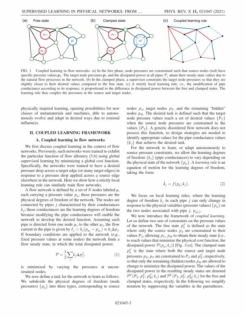
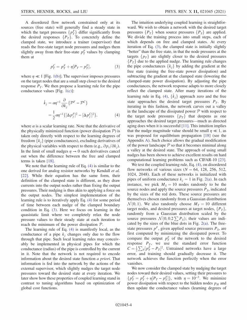
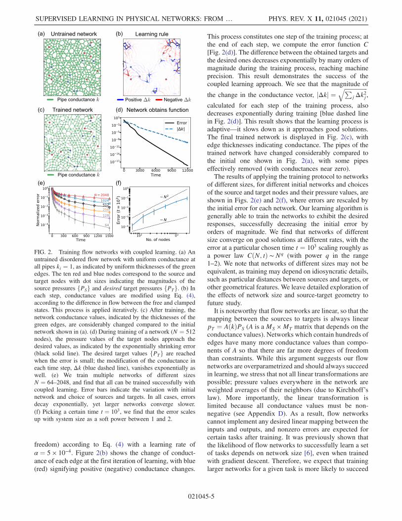
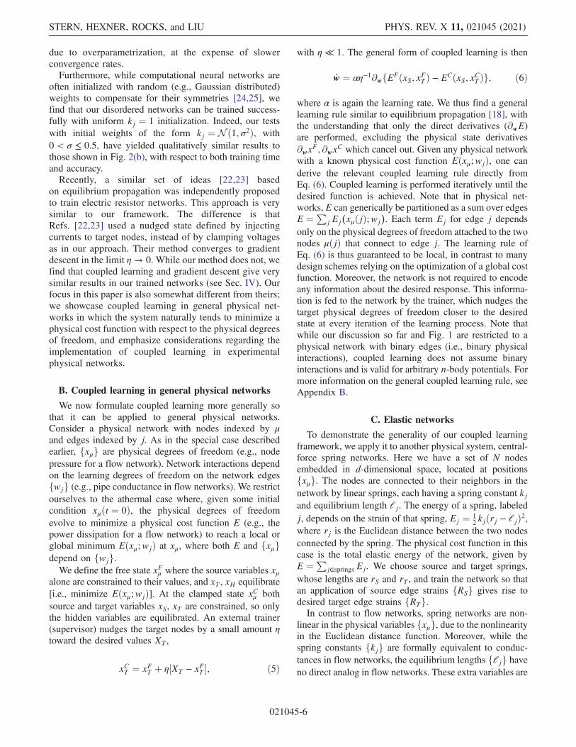
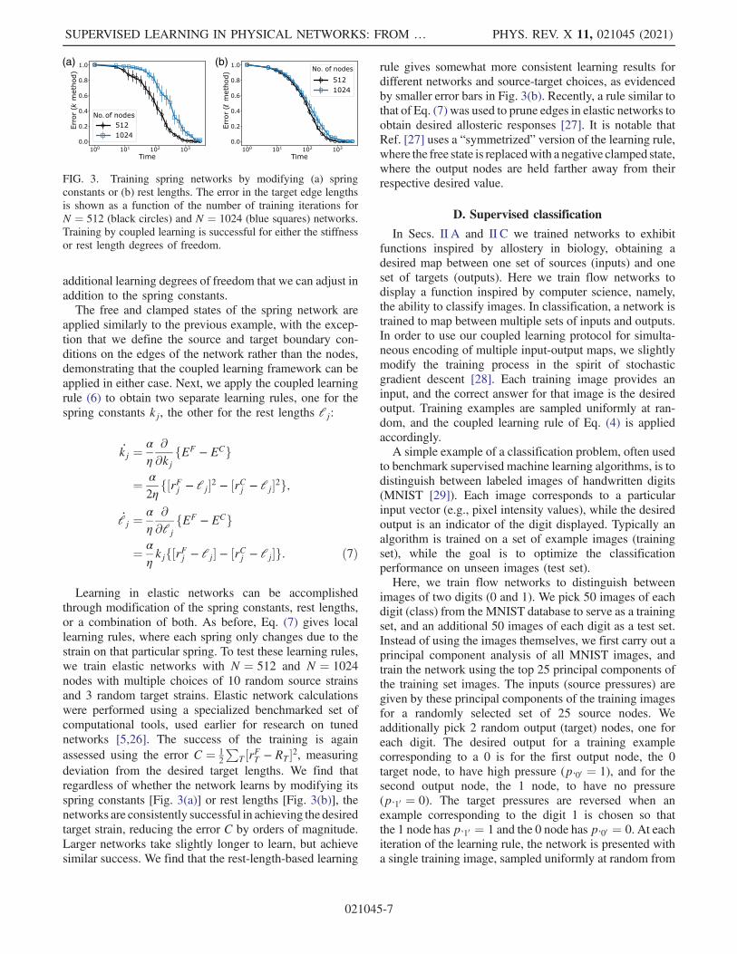
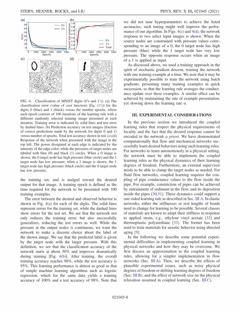
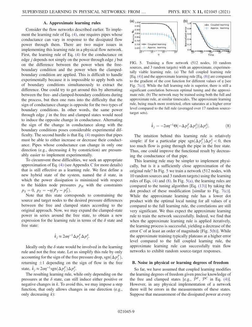
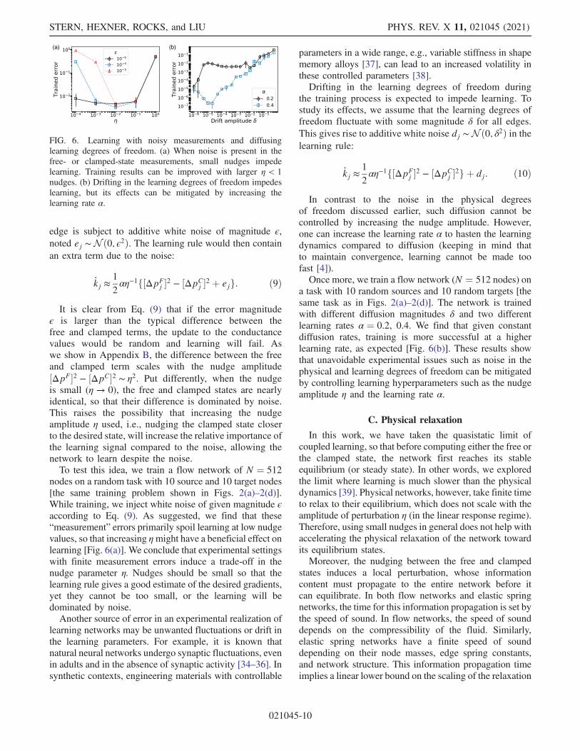
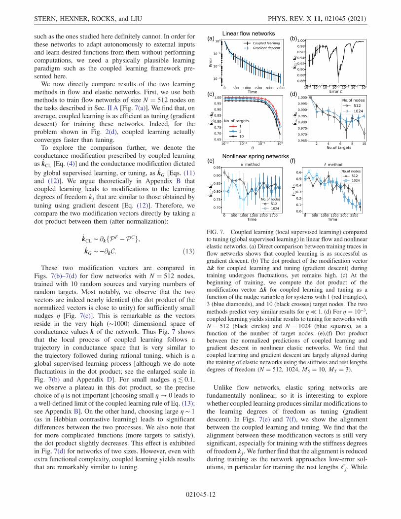
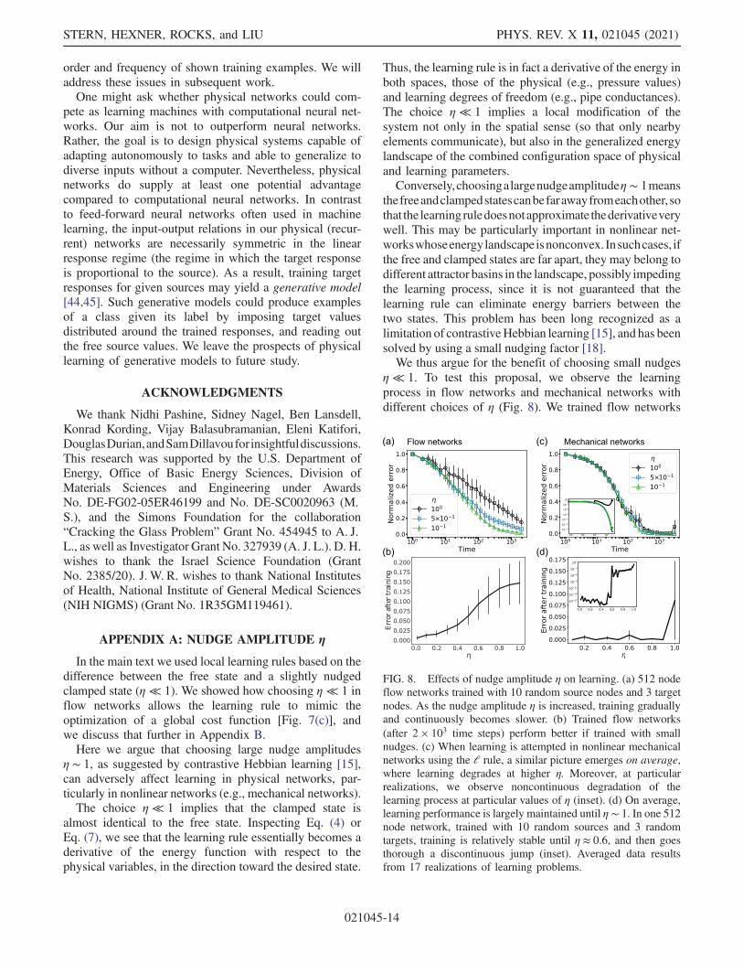
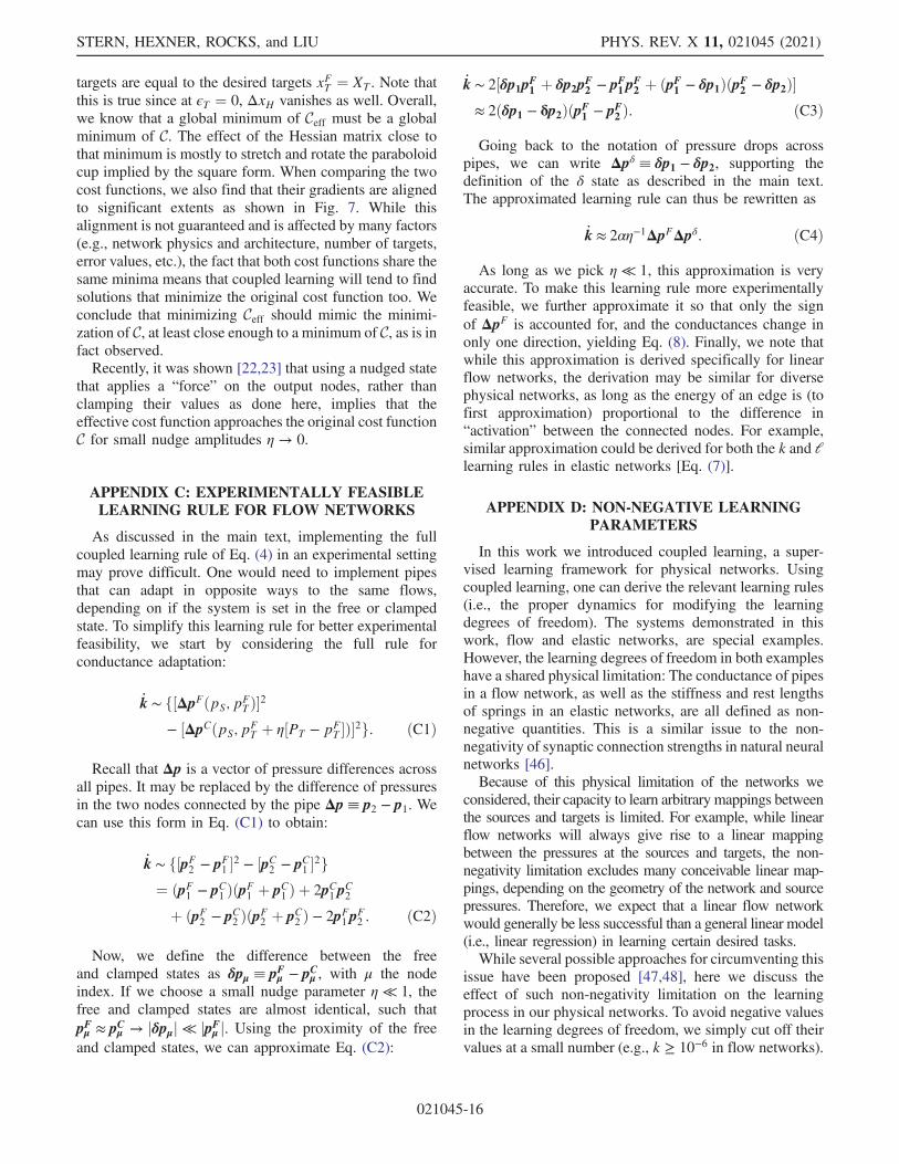
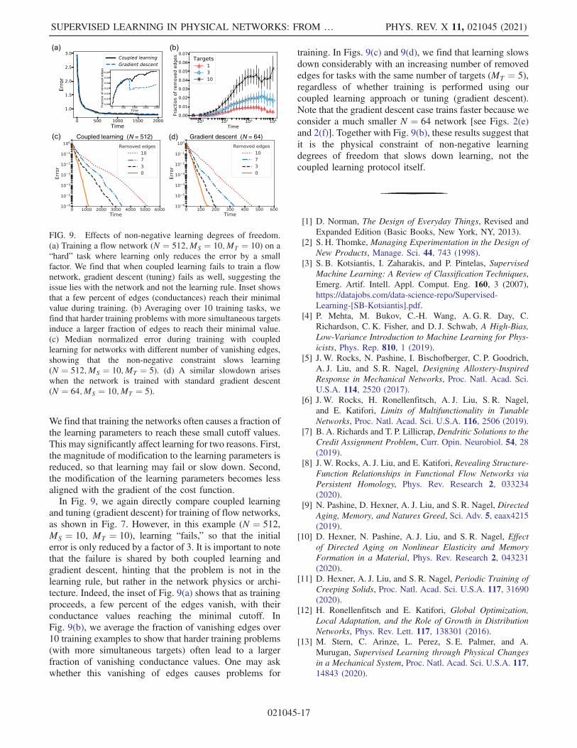