13 Machine Learning Supervised Decision Trees
113
Machine Learning for Data Mining Graphic Models Decision Trees Andres Mendez-Vazquez July 13, 2015 1 / 47
-
Upload
andres-mendez-vazquez -
Category
Engineering
-
view
291 -
download
4
Transcript of 13 Machine Learning Supervised Decision Trees

Machine Learning for Data MiningGraphic Models Decision Trees
Andres Mendez-Vazquez
July 13, 2015
1 / 47
Outline
1 IntroductionExamples
2 Decision TreesDecision TreesHow they workGeometryTypes of Decision Trees
3 Ordinary Binary Classification TreesDefinitionTrainingThe Sought CriterionsProbabilistic ImpurityFinal AlgorithmConclusions
2 / 47
Outline
1 IntroductionExamples
2 Decision TreesDecision TreesHow they workGeometryTypes of Decision Trees
3 Ordinary Binary Classification TreesDefinitionTrainingThe Sought CriterionsProbabilistic ImpurityFinal AlgorithmConclusions
3 / 47
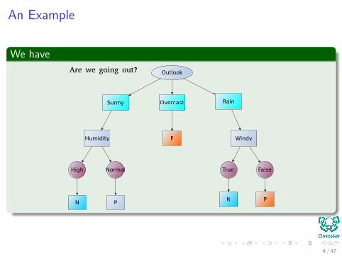
An Example
We haveOutlook
Sunny Overcast Rain
Humidity Windy
High Normal True False
N PN P
P
Are we going out?
4 / 47
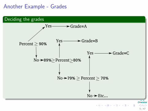
Another Example - Grades
Deciding the grades
Percent 90%
Yes Grade=A
Yes
Yes
No 89% Percent 80%
Grade=B
No 79% Percent 70%
Grade=C
No Etc...
5 / 47
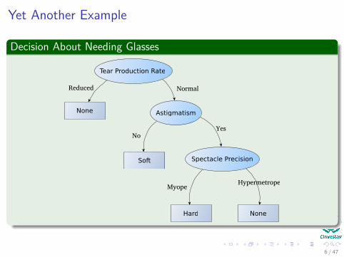
Yet Another Example
Decision About Needing Glasses
Tear Production Rate
None Astigmatism
Spectacle PrecisionSoft
Hard None
Reduced Normal
NoYes
MyopeHypermetrope
6 / 47
Outline
1 IntroductionExamples
2 Decision TreesDecision TreesHow they workGeometryTypes of Decision Trees
3 Ordinary Binary Classification TreesDefinitionTrainingThe Sought CriterionsProbabilistic ImpurityFinal AlgorithmConclusions
7 / 47
Decision Trees
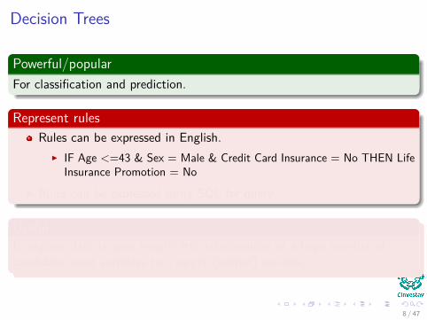
Powerful/popularFor classification and prediction.
Represent rulesRules can be expressed in English.
I IF Age <=43 & Sex = Male & Credit Card Insurance = No THEN LifeInsurance Promotion = No
Rules can be expressed using SQL for query.
Usefulto explore data to gain insight into relationships of a large number ofcandidate input variables to a target (output) variable.
8 / 47
Decision Trees
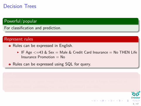
Powerful/popularFor classification and prediction.
Represent rulesRules can be expressed in English.
I IF Age <=43 & Sex = Male & Credit Card Insurance = No THEN LifeInsurance Promotion = No
Rules can be expressed using SQL for query.
Usefulto explore data to gain insight into relationships of a large number ofcandidate input variables to a target (output) variable.
8 / 47
Decision Trees
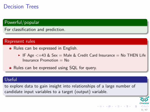
Powerful/popularFor classification and prediction.
Represent rulesRules can be expressed in English.
I IF Age <=43 & Sex = Male & Credit Card Insurance = No THEN LifeInsurance Promotion = No
Rules can be expressed using SQL for query.
Usefulto explore data to gain insight into relationships of a large number ofcandidate input variables to a target (output) variable.
8 / 47
Decision Trees
Powerful/popularFor classification and prediction.
Represent rulesRules can be expressed in English.
I IF Age <=43 & Sex = Male & Credit Card Insurance = No THEN LifeInsurance Promotion = No
Rules can be expressed using SQL for query.
Usefulto explore data to gain insight into relationships of a large number ofcandidate input variables to a target (output) variable.
8 / 47
Decision Trees - What is this?
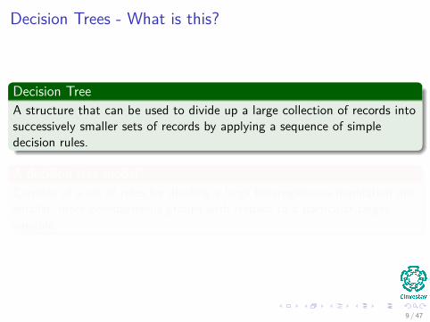
Decision TreeA structure that can be used to divide up a large collection of records intosuccessively smaller sets of records by applying a sequence of simpledecision rules.
A decision tree modelConsists of a set of rules for dividing a large heterogeneous population intosmaller, more homogeneous groups with respect to a particular targetvariable.
9 / 47
Decision Trees - What is this?
Decision TreeA structure that can be used to divide up a large collection of records intosuccessively smaller sets of records by applying a sequence of simpledecision rules.
A decision tree modelConsists of a set of rules for dividing a large heterogeneous population intosmaller, more homogeneous groups with respect to a particular targetvariable.
9 / 47
Decision Tree Types
Binary treesOnly two choices in each split. Can be non-uniform (uneven) in depth.
N-way trees or Ternary treesThree or more choices in at least one of its splits (3-way, 4-way, etc.).
10 / 47
Decision Tree Types
Binary treesOnly two choices in each split. Can be non-uniform (uneven) in depth.
N-way trees or Ternary treesThree or more choices in at least one of its splits (3-way, 4-way, etc.).
10 / 47
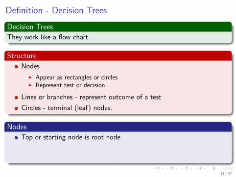
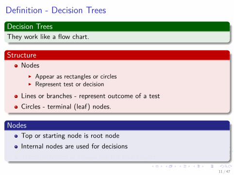
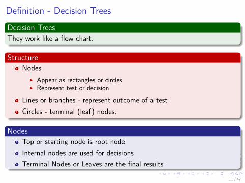
Definition - Decision TreesDecision TreesThey work like a flow chart.
StructureNodes
I Appear as rectangles or circlesI Represent test or decision
Lines or branches - represent outcome of a testCircles - terminal (leaf) nodes.
NodesTop or starting node is root nodeInternal nodes are used for decisionsTerminal Nodes or Leaves are the final results
11 / 47
Outline
1 IntroductionExamples
2 Decision TreesDecision TreesHow they workGeometryTypes of Decision Trees
3 Ordinary Binary Classification TreesDefinitionTrainingThe Sought CriterionsProbabilistic ImpurityFinal AlgorithmConclusions
12 / 47
How they work
How they work1 Decision rules - partition sample of data.2 Terminal node (leaf) indicates the class assignment.3 Tree partitions samples into mutually exclusive groups.4 One group for each terminal node.5 All paths:
1 Start at the root node.2 End at a leaf.
13 / 47
How they work
How they work1 Decision rules - partition sample of data.2 Terminal node (leaf) indicates the class assignment.3 Tree partitions samples into mutually exclusive groups.4 One group for each terminal node.5 All paths:
1 Start at the root node.2 End at a leaf.
13 / 47
How they work
How they work1 Decision rules - partition sample of data.2 Terminal node (leaf) indicates the class assignment.3 Tree partitions samples into mutually exclusive groups.4 One group for each terminal node.5 All paths:
1 Start at the root node.2 End at a leaf.
13 / 47
How they work
How they work1 Decision rules - partition sample of data.2 Terminal node (leaf) indicates the class assignment.3 Tree partitions samples into mutually exclusive groups.4 One group for each terminal node.5 All paths:
1 Start at the root node.2 End at a leaf.
13 / 47
How they work
How they work1 Decision rules - partition sample of data.2 Terminal node (leaf) indicates the class assignment.3 Tree partitions samples into mutually exclusive groups.4 One group for each terminal node.5 All paths:
1 Start at the root node.2 End at a leaf.
13 / 47
How they work
How they work1 Decision rules - partition sample of data.2 Terminal node (leaf) indicates the class assignment.3 Tree partitions samples into mutually exclusive groups.4 One group for each terminal node.5 All paths:
1 Start at the root node.2 End at a leaf.
13 / 47
How they work
How they work1 Decision rules - partition sample of data.2 Terminal node (leaf) indicates the class assignment.3 Tree partitions samples into mutually exclusive groups.4 One group for each terminal node.5 All paths:
1 Start at the root node.2 End at a leaf.
13 / 47
How they work (cont...)
Each path represents a decision ruleJoining (AND) of all the tests along that path.Separate paths that result in the same class are disjunctions (ORs).
All paths - mutually exclusiveFor any one case - only one path will be followed.False decisions on the left branch.True decisions on the right branch.
14 / 47
Outline
1 IntroductionExamples
2 Decision TreesDecision TreesHow they workGeometryTypes of Decision Trees
3 Ordinary Binary Classification TreesDefinitionTrainingThe Sought CriterionsProbabilistic ImpurityFinal AlgorithmConclusions
15 / 47
Geometry
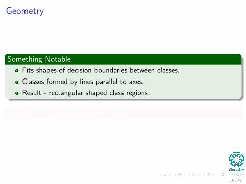
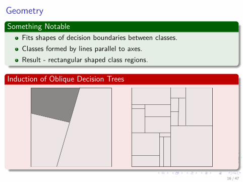
Something NotableFits shapes of decision boundaries between classes.Classes formed by lines parallel to axes.Result - rectangular shaped class regions.
Induction of Oblique Decision Trees
16 / 47
GeometrySomething Notable
Fits shapes of decision boundaries between classes.Classes formed by lines parallel to axes.Result - rectangular shaped class regions.
Induction of Oblique Decision Trees
16 / 47
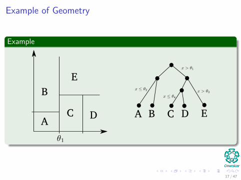
Example of Geometry
Example
A
B
C D
E
A B C D E
17 / 47
Outline
1 IntroductionExamples
2 Decision TreesDecision TreesHow they workGeometryTypes of Decision Trees
3 Ordinary Binary Classification TreesDefinitionTrainingThe Sought CriterionsProbabilistic ImpurityFinal AlgorithmConclusions
18 / 47
Types of Decision Trees
Classification TreesThe predicted outcome is the class to which the data belongs.
Regression TreesThe predicted outcome can be considered a number.
19 / 47
Types of Decision Trees
Classification TreesThe predicted outcome is the class to which the data belongs.
Regression TreesThe predicted outcome can be considered a number.
19 / 47
Classification and Regression Trees (CART)
CARTThe term CART is an umbrella term used to refer to both of theabove procedures.
Introduced byIt was introduced by Breiman et. al in the book
I “Classification and Regression Trees”
SimilaritiesRegression and Classification trees have some similarities –nevertheless they differ in the way the splitting at each node is done.
20 / 47
Ordinary Binary Classification Trees (OBCTs)
We will concentrate inOBCT Classification treesIf somebody want to look at more regression trees, look at“Classification and Regression Trees” by Breiman et. al .
21 / 47
Outline
1 IntroductionExamples
2 Decision TreesDecision TreesHow they workGeometryTypes of Decision Trees
3 Ordinary Binary Classification TreesDefinitionTrainingThe Sought CriterionsProbabilistic ImpurityFinal AlgorithmConclusions
22 / 47

Important
Most of the workIt focuses on deciding which property test or query should be performed atthe node!!!
If the data test is numerical in natureThere is a way to vizualize the decision boundaries produced by thedecision trees.
23 / 47
Important
Most of the workIt focuses on deciding which property test or query should be performed atthe node!!!
If the data test is numerical in natureThere is a way to vizualize the decision boundaries produced by thedecision trees.
23 / 47
Definition OBCT
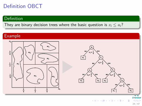
DefinitionThey are binary decision trees where the basic question is xi ≤ ai?
Example
24 / 47
Definition OBCT
DefinitionThey are binary decision trees where the basic question is xi ≤ ai?
Example
24 / 47
Outline
1 IntroductionExamples
2 Decision TreesDecision TreesHow they workGeometryTypes of Decision Trees
3 Ordinary Binary Classification TreesDefinitionTrainingThe Sought CriterionsProbabilistic ImpurityFinal AlgorithmConclusions
25 / 47
Training of a OBCT
We need firstAt each node, the set of candidate questions to be asked has to bedecided.Each question corresponds to a specific binary split into twodescendant nodes.Each node, t, is associated with a specific subset Xt of the trainingset X .
26 / 47
Training of a OBCT
We need firstAt each node, the set of candidate questions to be asked has to bedecided.Each question corresponds to a specific binary split into twodescendant nodes.Each node, t, is associated with a specific subset Xt of the trainingset X .
26 / 47
Training of a OBCT
We need firstAt each node, the set of candidate questions to be asked has to bedecided.Each question corresponds to a specific binary split into twodescendant nodes.Each node, t, is associated with a specific subset Xt of the trainingset X .
26 / 47
Splitting the Node Xt
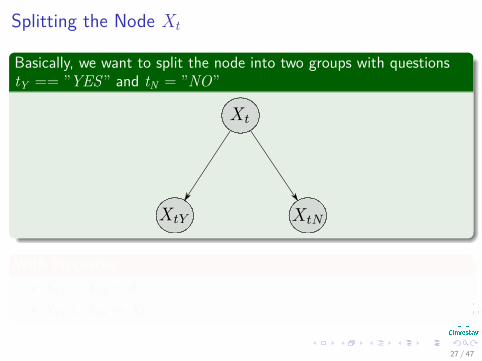
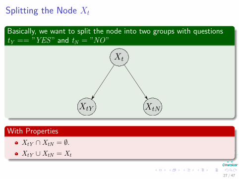
Basically, we want to split the node into two groups with questionstY == ”YES” and tN = ”NO”
With PropertiesXtY ∩XtN = ∅.XtY ∪XtN = Xt
27 / 47
Splitting the Node Xt
Basically, we want to split the node into two groups with questionstY == ”YES” and tN = ”NO”
With PropertiesXtY ∩XtN = ∅.XtY ∪XtN = Xt
27 / 47
Important
Given the question for each feature k “Is xk ≤ α”For each feature, every possible value of the threshold α defines a specificsplit of the subset Xt .
Thus in theoryAn infinite set of questions has to be asked if α is an interval Yα ⊆ R.
In practiceonly a finite set of questions can be considered.
28 / 47
For example
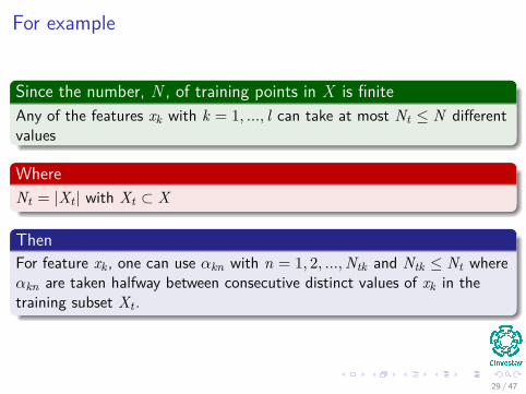
Since the number, N , of training points in X is finiteAny of the features xk with k = 1, ..., l can take at most Nt ≤ N differentvalues
WhereNt = |Xt | with Xt ⊂ X
ThenFor feature xk , one can use αkn with n = 1, 2, ...,Ntk and Ntk ≤ Nt whereαkn are taken halfway between consecutive distinct values of xk in thetraining subset Xt .
29 / 47
For example
Since the number, N , of training points in X is finiteAny of the features xk with k = 1, ..., l can take at most Nt ≤ N differentvalues
WhereNt = |Xt | with Xt ⊂ X
ThenFor feature xk , one can use αkn with n = 1, 2, ...,Ntk and Ntk ≤ Nt whereαkn are taken halfway between consecutive distinct values of xk in thetraining subset Xt .
29 / 47
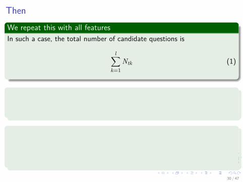
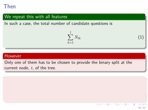
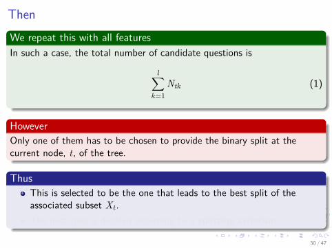
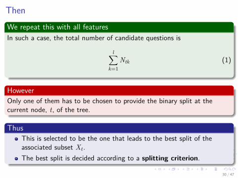
ThenWe repeat this with all featuresIn such a case, the total number of candidate questions is
l∑k=1
Ntk (1)
HoweverOnly one of them has to be chosen to provide the binary split at thecurrent node, t, of the tree.
ThusThis is selected to be the one that leads to the best split of theassociated subset Xt .The best split is decided according to a splitting criterion.
30 / 47
Outline
1 IntroductionExamples
2 Decision TreesDecision TreesHow they workGeometryTypes of Decision Trees
3 Ordinary Binary Classification TreesDefinitionTrainingThe Sought CriterionsProbabilistic ImpurityFinal AlgorithmConclusions
31 / 47
Criterions to be found
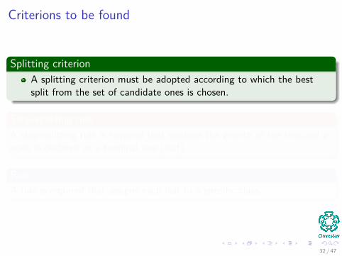
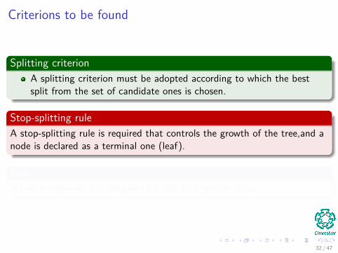
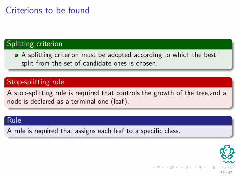
Splitting criterionA splitting criterion must be adopted according to which the bestsplit from the set of candidate ones is chosen.
Stop-splitting ruleA stop-splitting rule is required that controls the growth of the tree,and anode is declared as a terminal one (leaf).
RuleA rule is required that assigns each leaf to a specific class.
32 / 47
Criterions to be found
Splitting criterionA splitting criterion must be adopted according to which the bestsplit from the set of candidate ones is chosen.
Stop-splitting ruleA stop-splitting rule is required that controls the growth of the tree,and anode is declared as a terminal one (leaf).
RuleA rule is required that assigns each leaf to a specific class.
32 / 47
Looking for Homogeneity!!!
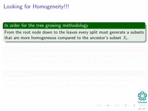
In order for the tree growing methodologyFrom the root node down to the leaves every split must generate a subsetsthat are more homogeneous compared to the ancestor’s subset Xt .
MeaningThe training feature vectors in each one of the new subsets show, whereasdata in Xt are more equally distributed among the classes.
For exampleConsider the task of classifying four classes and assume that the vectors insubset Xt are distributed among the classes with equal probability.
33 / 47
Looking for Homogeneity!!!
In order for the tree growing methodologyFrom the root node down to the leaves every split must generate a subsetsthat are more homogeneous compared to the ancestor’s subset Xt .
MeaningThe training feature vectors in each one of the new subsets show, whereasdata in Xt are more equally distributed among the classes.
For exampleConsider the task of classifying four classes and assume that the vectors insubset Xt are distributed among the classes with equal probability.
33 / 47
Thus
If we split the node soω1 and ω2 form XtY
ω3 and ω4 form XtN
ThenXtY and XtN are more homogeneous compared to Xt .
In other words“Purer” in the decision tree terminology.
34 / 47
Thus
If we split the node soω1 and ω2 form XtY
ω3 and ω4 form XtN
ThenXtY and XtN are more homogeneous compared to Xt .
In other words“Purer” in the decision tree terminology.
34 / 47
Thus
If we split the node soω1 and ω2 form XtY
ω3 and ω4 form XtN
ThenXtY and XtN are more homogeneous compared to Xt .
In other words“Purer” in the decision tree terminology.
34 / 47
Our Goal
We needTo define a measure that quantifies node impurity.
ThusThe Overall Impurity of the descendant nodes is optimally decreased withrespect to the ancestor node’s impurity.
35 / 47
Our Goal
We needTo define a measure that quantifies node impurity.
ThusThe Overall Impurity of the descendant nodes is optimally decreased withrespect to the ancestor node’s impurity.
35 / 47
Outline
1 IntroductionExamples
2 Decision TreesDecision TreesHow they workGeometryTypes of Decision Trees
3 Ordinary Binary Classification TreesDefinitionTrainingThe Sought CriterionsProbabilistic ImpurityFinal AlgorithmConclusions
36 / 47
Probabilistic Impurity
Assume the following probability of a vector in Xt belongs to class ωi
P(ωi |t) for i = 1, · · · ,M (2)
37 / 47
Probabilistic Impurity
Assume the following probability of a vector in Xt belongs to class ωi
P(ωi |t) for i = 1, · · · ,M (2)
37 / 47
A Common Impurity
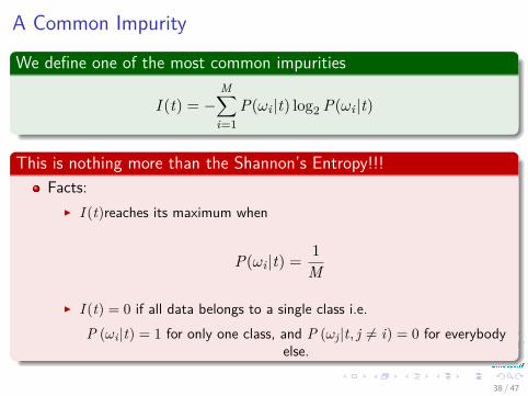
We define one of the most common impurities
I (t) = −M∑
i=1P(ωi |t) log2 P(ωi |t)
This is nothing more than the Shannon’s Entropy!!!Facts:
I I (t)reaches its maximum when
P(ωi |t) = 1M
I I (t) = 0 if all data belongs to a single class i.e.P (ωi |t) = 1 for only one class, and P (ωj |t, j 6= i) = 0 for everybody
else.
38 / 47

A Common Impurity
We define one of the most common impurities
I (t) = −M∑
i=1P(ωi |t) log2 P(ωi |t)
This is nothing more than the Shannon’s Entropy!!!Facts:
I I (t)reaches its maximum when
P(ωi |t) = 1M
I I (t) = 0 if all data belongs to a single class i.e.P (ωi |t) = 1 for only one class, and P (ωj |t, j 6= i) = 0 for everybody
else.
38 / 47
In reality...
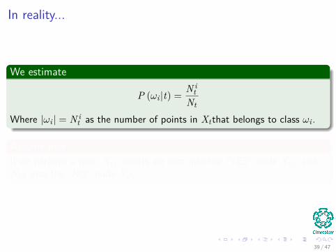
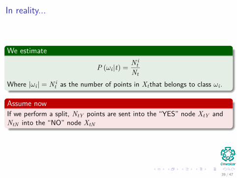
We estimate
P (ωi |t) = N it
Nt
Where |ωi | = N it as the number of points in Xtthat belongs to class ωi .
Assume nowIf we perform a split, NtY points are sent into the “YES” node XtY andNtN into the “NO” node XtN
39 / 47
In reality...
We estimate
P (ωi |t) = N it
Nt
Where |ωi | = N it as the number of points in Xtthat belongs to class ωi .
Assume nowIf we perform a split, NtY points are sent into the “YES” node XtY andNtN into the “NO” node XtN
39 / 47
Decrease in node impurity
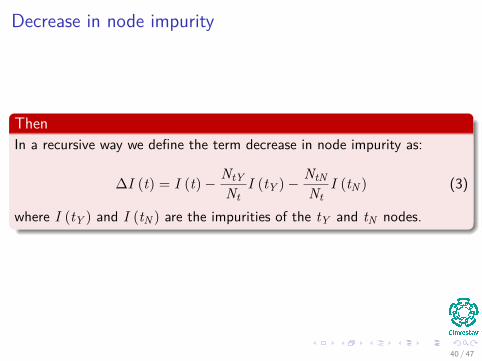
ThenIn a recursive way we define the term decrease in node impurity as:
∆I (t) = I (t)− NtYNt
I (tY )− NtNNt
I (tN ) (3)
where I (tY ) and I (tN ) are the impurities of the tY and tN nodes.
40 / 47
The Final Goal
The Final GoalTo adopt from the set of candidate questions the one that performs thesplit with the highest decrease of impurity.
41 / 47
Stop-Splitting Rule
NowThe natural question that now arises is when one decides to stop splittinga node and declares it as a leaf of the tree.
For example you can adoptA threshold T and stop splitting if the maximum value of ∆I (t) over allpossible splits is less than T .
Other posibilitiesIf the subset Xt is small enough.If the subset Xt is pure, in the sense that all points in it belong to asingle class.
42 / 47
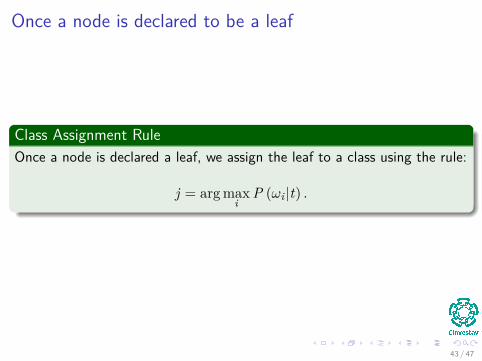
Once a node is declared to be a leaf
Class Assignment RuleOnce a node is declared a leaf, we assign the leaf to a class using the rule:
j = arg maxi
P (ωi |t) .
43 / 47
Outline
1 IntroductionExamples
2 Decision TreesDecision TreesHow they workGeometryTypes of Decision Trees
3 Ordinary Binary Classification TreesDefinitionTrainingThe Sought CriterionsProbabilistic ImpurityFinal AlgorithmConclusions
44 / 47

Final Algorithm
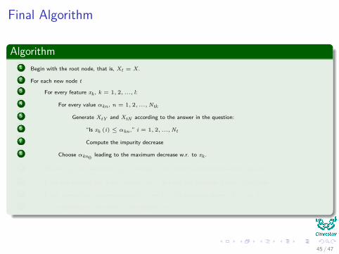
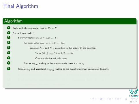
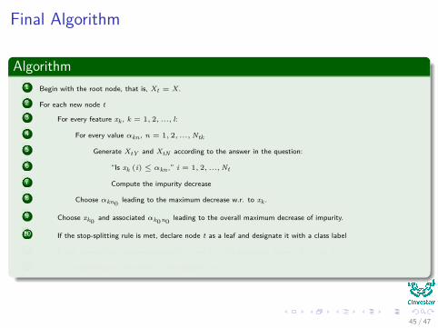
Algorithm1 Begin with the root node, that is, Xt = X.
2 For each new node t
3 For every feature xk , k = 1, 2, ..., l:
4 For every value αkn , n = 1, 2, ...,Ntk
5 Generate XtY and XtN according to the answer in the question:
6 “Is xk (i) ≤ αkn ,” i = 1, 2, ...,Nt
7 Compute the impurity decrease
8 Choose αkn0 leading to the maximum decrease w.r. to xk .
9 Choose xk0 and associated αk0n0 leading to the overall maximum decrease of impurity.
10 If the stop-splitting rule is met, declare node t as a leaf and designate it with a class label
11 If not, generate two descendant nodes tY and tN with associated subsets XtY and XtN ,
12 depending on the answer to the question: is xk0 ≤ α?
45 / 47

Final Algorithm
Algorithm1 Begin with the root node, that is, Xt = X.
2 For each new node t
3 For every feature xk , k = 1, 2, ..., l:
4 For every value αkn , n = 1, 2, ...,Ntk
5 Generate XtY and XtN according to the answer in the question:
6 “Is xk (i) ≤ αkn ,” i = 1, 2, ...,Nt
7 Compute the impurity decrease
8 Choose αkn0 leading to the maximum decrease w.r. to xk .
9 Choose xk0 and associated αk0n0 leading to the overall maximum decrease of impurity.
10 If the stop-splitting rule is met, declare node t as a leaf and designate it with a class label
11 If not, generate two descendant nodes tY and tN with associated subsets XtY and XtN ,
12 depending on the answer to the question: is xk0 ≤ α?
45 / 47
Outline
1 IntroductionExamples
2 Decision TreesDecision TreesHow they workGeometryTypes of Decision Trees
3 Ordinary Binary Classification TreesDefinitionTrainingThe Sought CriterionsProbabilistic ImpurityFinal AlgorithmConclusions
46 / 47
Conclusions
RemarkDecision trees have emerged as one of the most popular methods ofclassification.
RemarkA variety of node impurity measures can be defined.
RemarkThe size of the three need to be controlled. The threshold T leadsincorrect sizes.
RemarkA drawback associated with tree classifiers is their high variance.Different training data set results in a very different tree.
47 / 47