Suitability Analysis Guidebook/Training Materials : Manual...

5-5667-01-P3

Suitability Analysis Guidebook/Training Materials: Manual for Application of Suitability Analysis for a Selected Region in Texas Authors: Dr. Ardeshir Anjomani Ali Tayebi Dian Nostikasari Gehendra Kharel Project 5-5667-01: Implementation of Accessible Land Use Modeling Tools for Texas Applications AUGUST 31, 2010

Performing Organization: University of Texas at Arlington School of Urban and Public Affairs (SUPA) Box 19588 Arlington, TX 76019

Sponsoring Organization: Texas Department of Transportation Research and Technology Implementation Office P.O. Box 5080 Austin, Texas 78763-5080

Performed in cooperation with the Texas Department of Transportation and the Federal Highway Administration.

iii

Table of Contents Section I: Background and Application Process ........................................................................ 1 1. Background ............................................................................................................................. 1 2. Study Area .............................................................................................................................. 1 3. Process .................................................................................................................................... 1

Projection of Employment and Household ................................................................................. 1

3.1.1 Data ........................................................................................................................... 1

3.1.2 Employment Classification ....................................................................................... 2

3.1.3 Household Classification .......................................................................................... 4

Required Land ............................................................................................................................. 5

3.1.4 Required Land for Employment ............................................................................... 5

3.1.5 Required Land for Household ................................................................................... 7

Suitability Analysis ..................................................................................................................... 8

3.1.6 Selection of Suitability Factors ................................................................................. 8

3.1.7 Selection of Land uses .............................................................................................. 8

3.1.8 Suitability Factors’ Categories .................................................................................. 9

3.1.9 Rating ...................................................................................................................... 10

3.1.10 Weighting ................................................................................................................ 11

Allocation of Employment and Households ............................................................................. 16

Section II: Prototype Model and Step-by-Step Process ........................................................... 17 4. Running the SA Model Toolbox in ArcGIS ......................................................................... 17

Rating Toolset ........................................................................................................................... 18

4.1.1 Proximity................................................................................................................. 18

4.1.2 Accessibility ............................................................................................................ 18

4.1.3 Assignment ............................................................................................................. 19

Weighting Toolset ..................................................................................................................... 20

4.1.4 Mask for Each Land Use......................................................................................... 20

4.1.5 Suitability for Each Land Use ................................................................................. 21

Allocation Toolset ..................................................................................................................... 22

4.1.6 Combine the Suitability Layers .............................................................................. 22

4.1.7 Allocating ................................................................................................................ 23

4.1.8 Compare Scenarios ................................................................................................. 24

4.1.9 TAZ ......................................................................................................................... 26

Appendix A: Proximity Tool ........................................................................................................ 31

Highway ................................................................................................................................ 31

iv

Endangered Species .............................................................................................................. 33

Water Bodies ......................................................................................................................... 35

Wetlands ............................................................................................................................... 37

Appendix B: Accessibility Tool .................................................................................................... 39

Airport ................................................................................................................................... 39

Employment Centers ............................................................................................................. 40

Intersection ............................................................................................................................ 42

Shopping Centers .................................................................................................................. 43

Appendix C: Assignment Tool ..................................................................................................... 45

Land Use ............................................................................................................................... 45

Karst ...................................................................................................................................... 47

TEAP..................................................................................................................................... 48

Appendix D: Allocation Toolset ................................................................................................... 51

Open Space ........................................................................................................................... 53

Single Family (SF) 2010 ....................................................................................................... 54

Multi Family (MF) ................................................................................................................ 55

Basic Heavy Industrial (BHI) ............................................................................................... 56

Basic Light Industrial (BLI) .................................................................................................. 57

Service Heavy Industrial (SHI) ............................................................................................. 58

Service Light Industrial (SLI) ............................................................................................... 59

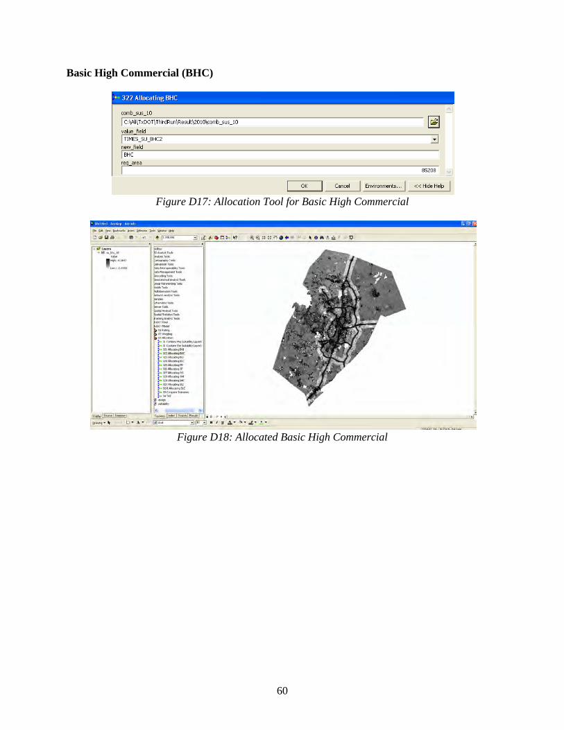
Basic High Commercial (BHC) ............................................................................................ 60

Basic Low Commercial (BLC) ............................................................................................. 61

Service High Commercial (SHC) ......................................................................................... 62

Service Low Commercial ..................................................................................................... 63

Appendix E: Suitability Tool ........................................................................................................ 65

Suitability for 2005 ............................................................................................................... 65

Suitability for 2010 ............................................................................................................... 66

v

List of Figures Figure 3.1: Screenshot of Rating Table in Microsoft Office Access ............................................ 11 Figure 3.2: Screenshot of the AHP Weighting Table in Microsoft Office Access ....................... 11 Figure 3.3: Screenshot of Download Page .................................................................................... 12 Figure 3.4: Customize Option in the Tools Menu ........................................................................ 12 Figure 3.5: Adding the AHP Extension ........................................................................................ 13 Figure 3.6: Adding AHP Toolbar ................................................................................................. 13 Figure 3.7: AHP Toolbar .............................................................................................................. 13 Figure 3.8: Defining Criteria (Factors) for Weighting .................................................................. 14 Figure 3.9: Adding Description to the Criteria ............................................................................. 14 Figure 3.10: Pair-wise Comparison in AHP ................................................................................. 15 Figure 3.11: AHP Result ............................................................................................................... 15 Figure 3.12: Entering AHP Result into the Weighting Toolset .................................................... 16 Figure 4.1: Adding the Model Toolbox ........................................................................................ 17 Figure 4.2: The Model in ArcToolbox .......................................................................................... 17 Figure 4.3: Example of Proximity Tool (Proximity to Highway) ................................................ 18 Figure 4.4: Example of Accessibility Tool (Accessibility to Airport) .......................................... 19 Figure 4.5: Example of Assignment Tool (Land Use Rating Layer) ............................................ 20 Figure 4.6: Mask Tool for Each Land Use ................................................................................... 21 Figure 4.7: Result of the Mask Tool ............................................................................................. 21 Figure 4.8: Suitability for Each Land Use Tool ............................................................................ 22 Figure 4.9: Combine the Suitability Layers Tool ......................................................................... 23 Figure 4.10: Example of Allocation Tool (Allocating BHI) ......................................................... 24 Figure 4.11: Adding Scenario 1 Result in Compare Scenarios Tool ............................................ 25 Figure 4.12: Adding Scenario 2 Result in Compare Scenario Tool ............................................. 25 Figure 4.13: Specifying Name and Location of Result ................................................................. 26 Figure 4.14: Net Gain/Loss of Development due to Scenario Change ......................................... 26 Figure 4.15: TAZ Tool .................................................................................................................. 27 Figure 4.16: TAZ Attribute Field .................................................................................................. 27 Figure 4.17: Select all the Fields in the Attribute Table and Copy to Microsoft Excel ................ 28 Figure 4.18: Join the Excel Sheet with TAZ Shapefile ................................................................ 29 Figure 4.19: Add New Field to the TAZ Attribute Table ............................................................. 29 Figure 4.20: Calculate Area in Acre ............................................................................................. 30 Figure 4.21: Calculate Employment Density in Field Calculator ................................................. 30 Figure A1: Proximity to Highway Tool ........................................................................................ 31 Figure A2: Result of Proximity to Highway Tool ........................................................................ 32 Figure A3: Result (Zoomed In) of Proximity to Highway Tool ................................................... 33 Figure A4: Proximity to Endangered Species Tool ...................................................................... 33 Figure A5: Result of Proximity to Endangered Species Tool ....................................................... 34 Figure A6: Proximity to Water Bodies Tool ................................................................................. 35 Figure A7: Result of Proximity to Water Bodies Tool ................................................................. 36 Figure A8: Proximity to Wetlands Tool ....................................................................................... 37 Figure A9: Result of Proximity to Wetland Tool ......................................................................... 38 Figure B1: Accessibility to Airport Tool ...................................................................................... 39

vi

Figure B2: Result of Accessibility to Airport Tool ...................................................................... 40 Figure B3: Accessibility to Employment Centers Tool ................................................................ 40 Figure B4: Result of Accessibility to Employment Centers Tool ................................................ 41 Figure B5: Accessibility to Intersection Tool ............................................................................... 42 Figure B6: Result of Accessibility to Intersection Tool ............................................................... 43 Figure B7: Accessibility to Shopping Centers Tool ..................................................................... 43 Figure B8: Result of Accessibility to Shopping Centers Tool ...................................................... 44 Figure C1: Assignment Tool for Land Use................................................................................... 45 Figure C2: Result of Assignment of Land Use Tool .................................................................... 46 Figure C3: Assignment Tool for Karst ......................................................................................... 47 Figure C4: Result of Assignment of Karst Tool ........................................................................... 48 Figure C5: Assignment Tool for TEAP ........................................................................................ 49 Figure C6: Result of Assignment of TEAP Tool .......................................................................... 50 Figure D1: Allocation Tool to Combine Suitability Layers ......................................................... 51 Figure D2: Result of Allocation Tool Showing Available Land for Development ...................... 52 Figure D3: Allocation Tool for Open Space ................................................................................. 53 Figure D4: Allocated Open Space ................................................................................................ 53 Figure D5: Allocation Tool for Single Family ............................................................................. 54 Figure D6: Allocated Single Family ............................................................................................. 54 Figure D7: Allocation Tool for Multi Family ............................................................................... 55 Figure D8: Allocated Multi Family .............................................................................................. 55 Figure D9: Allocation Tool for Basic Heavy Industrial ............................................................... 56 Figure D10: Allocated Basic Heavy Industrial ............................................................................. 56 Figure D11: Allocation Tool for Basic Light Industrial ............................................................... 57 Figure D12: Allocated Basic Light Industrial ............................................................................... 57 Figure D13: Allocation Tool for Service Heavy Industrial .......................................................... 58 Figure D14: Allocated Service Heavy Industrial .......................................................................... 58 Figure D15: Allocation Tool for Service Light Industrial ............................................................ 59 Figure D16: Allocated Service Light Industrial ............................................................................ 59 Figure D17: Allocation Tool for Basic High Commercial ........................................................... 60 Figure D18: Allocated Basic High Commercial ........................................................................... 60 Figure D19: Allocation Tool for Basic Low Commercial ............................................................ 61 Figure D20: Allocated Basic Low Commercial ............................................................................ 61 Figure D21: Allocation Tool for Service High Commercial ........................................................ 62 Figure D22: Allocated Service High Commercial ........................................................................ 62 Figure D23: Allocation Tool for Service Low Commercial ......................................................... 63 Figure D24: Allocated Service Low Commercial ........................................................................ 63 Figure E1: Suitability Tool ........................................................................................................... 65 Figure E2: Suitability Tool for 2005 ............................................................................................. 65 Figure E3: Result Suitability 2005 ................................................................................................ 66 Figure E4: Result Suitability 2010 ................................................................................................ 66 Figure E5: Result Suitability Single Family 2010 ........................................................................ 67

vii

List of Tables Table 3.1: Data Types and Sources ................................................................................................. 1 Table 3.2: Employment Categories in Percentage .......................................................................... 2 Table 3.3: Average Area per Employment ..................................................................................... 3 Table 3.4: Basic and Service Employment in Hays County ........................................................... 4 Table 3.5: Household Categories .................................................................................................... 4 Table 3.6: Households in Hays County .......................................................................................... 5 Table 3.7: Households of the Study Area ....................................................................................... 5 Table 3.8: Required Land for Employment in Hays County .......................................................... 6 Table 3.9: Required Land for Employment in the Study Area ....................................................... 7 Table 3.10: Formula from Regression Analysis ............................................................................. 7 Table 3.11: Total Required Land .................................................................................................... 8 Table 3.12: Selected Suitability Factors ......................................................................................... 8 Table 3.13: Selected Land Uses ...................................................................................................... 9 Table 3.14: Suitability Factors’ Categories .................................................................................. 10 Table 3.15: Sample Rating Table .................................................................................................. 10 Table A1: Rating Table for Proximity to Highway ...................................................................... 32 Table A2: Rating Table for Endangered Species .......................................................................... 34 Table A3: Rating Table for Water Bodies .................................................................................... 36 Table A4: Rating Table for Wetlands ........................................................................................... 37 Table B1: Rating Table for Airport .............................................................................................. 40 Table B2: Rating Table for Employment Centers ........................................................................ 41 Table B3: Rating Table for Intersection ....................................................................................... 42 Table B4: Rating Table for Shopping Centers .............................................................................. 44 Table C1: Rating Table for Existing Land Use ............................................................................ 46 Table C2: Rating Table for Karst.................................................................................................. 47 Table C3: Rating Table for TEAP ................................................................................................ 49

1

Section I: Background and Application Process

1. Background This Guidebook is prepared as part of Task 2 of implementation project 5-5667, which focuses on the development of a prototype application of the Suitability Analysis model using GIS for a selected region in Texas. It is organized into two sections. Section I provides a description of the study area and background information on data collection and analysis process. Section II introduces a prototype model with a step-by-step process to run it. Appendices to the Guidebook give additional details about each component of the model along with the required data and GIS tools to run the model, and results of each step.

2. Study Area We selected the Austin Region for the development of a prototype application model using Suitability Analysis. The study region is comprised of three counties (Hays, Travis, and Williamson) out of the five counties that are within the Austin–Round Rock–San Marcos metropolitan area.

3. Process As mentioned in the report, this model follows a four-step process.

1) Projection of Employment and Households

2) Calculation of Required Land

3) Suitability Analysis

4) Allocation of Employment and Households

Projection of Employment and Household

3.1.1 Data Table 3.1 shows types of employment and household data with their sources collected for this study.

Table 3.1: Data Types and Sources Data Type Year Source

Population and households 2005 U.S. Census Bureau Population and households 2014 projected ESRI Population 2005-2040 projected Texas State Data Center Average parcel size for each land use CAPCOG data clearinghouse

Total employment projections Austin’s Capital Area Metropolitan Planning Organization (CAMPO)

Employment (2 digit NAICS) 2009 Texas Comptroller Office Employment Estimation (4 digit NAICS) 2006 Texas Workforce Commission Employment Projection (4 digit NAICS) 2016 Texas Workforce Commission Employment Estimation (2 digit NAICS) 2008 ESRI Business Analyst Employment Projection (2 digit NAICS) 2013 ESRI Business Analyst

2

After collecting required data for employment and household, this data was classified into different categories.

3.1.2 Employment Classification For this study purpose, 17 categories of employment were developed based on the data collected from Texas Workforce Commission for 2006. This report consolidated 4-digit NAICS codes into the 2-digit NAICS categories. Table 3.2 shows 2-digit NAICS employment categories with percentage of employees in each category for all three counties (Hays, Travis, and Williamson) for 2006. The purpose of showing employment categories in percentage is to break down total projected employment data from CAMPO into 2-digit NAICS categories for each projection year.

Table 3.2: Employment Categories in Percentage Employment Categories Employment Percentage

Hays Travis Williamson Accommodation and Food Services 7.80 8.30 7.80 Administrative and Support and Waste Management and Remediation Services

6.30 14.80 6.30

Agriculture, Forestry, Fishing and Hunting 0.80 0.10 0.80 Arts, Entertainment, and Recreation 1.50 1.90 1.50 Construction 15.30 10.6 15.30 Educational Services 47.50 37.40 47.50 Finance and Insurance 3.00 3.20 3.00 Health Care and Social Assistance 3.50 3.90 3.50 Information 0.00 0.60 0.00 Manufacturing 3.50 7.20 3.50 Other Services (except Public Administration) 1.60 1.60 1.60 Professional, Scientific, and Technical Services 1.70 3.60 1.70 Real Estate and Rental and Leasing 0.40 0.70 0.40 Retail Trade 6.90 4.90 6.90 Transportation and Warehousing 0.00 0.60 0.00 Utilities 0.3 0.00 0.3 Wholesale Trade 0.40 0.50 0.40 Total 100% 100% 100% Average area per employee needs to be calculated to find out how much land would be required for projected employment. Average area per employee was calculated by dividing the existing area with the number of employees in every 2-digit NAICS category. Table 3.3 shows average area per employment in square foot for Hays County. Average area for Travis and Williamson County can be calculated similarly.

3

Table 3.3: Average Area per Employment

Employment Categories Number of

Employment Area

(Sq.Ft)

Area per Employment

(Sq.Ft) Accommodation and Food Services 4,786 2,548,750 532.54 Administrative and Support and Waste Management and Remediation Services

587 776,250 1,322.40

Agriculture, Forestry, Fishing and Hunting 101 296,250 2,933.17 Arts, Entertainment, and Recreation 637 1,032,500 1,620.88 Construction 3,238 3,520,000 1,087.09 Educational Services 5,460 4,170,000 763.74 Finance and Insurance 753 940,000 1,248.34 Health Care and Social Assistance 3,537 3,395,000 959.85 Information 630 1,250,000 1,984.13 Manufacturing 3,413 3,562,500 1,007.14 Other Services (except Public Administration) 1,894 3,958,750 2,090.15 Professional, Scientific, and Technical Services 1,626 2,377,500 1,462.18 Real Estate and Rental and Leasing 1,215 3,133,750 2,579.22 Retail Trade 1,928 1,711,250 887.58 Transportation and Warehousing 665 1,088,750 1,637.22 Utilities 157 487,500 3,105.10 Wholesale Trade 1,810 3,157,500 1,744.48

Employment was categorized into basic and service sectors using the result of Location Quotient Technique. The following formula was used to calculate the number of basic sector employment for Hays County. The same formula can be used to calculate the number of basic sector employment for other counties or areas.

Basic Sector Employment = Hays County Employment IndustryTexas Employment Industry − Total Hays County EmploymentTotal Texas Employment × Texas Employment Industry

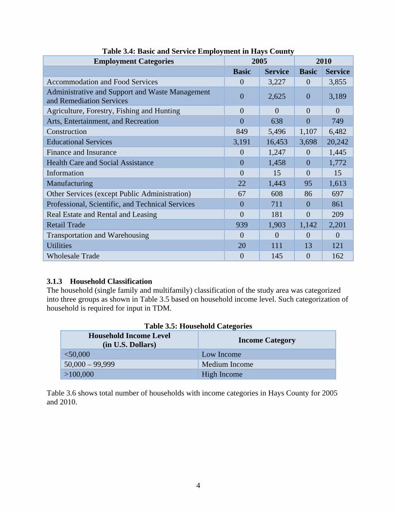
Table 3.4 shows basic and service sector employment in Hays County for the year 2005 and 2010.

4

Table 3.4: Basic and Service Employment in Hays County Employment Categories 2005 2010

Basic Service Basic ServiceAccommodation and Food Services 0 3,227 0 3,855 Administrative and Support and Waste Management and Remediation Services

0 2,625 0 3,189

Agriculture, Forestry, Fishing and Hunting 0 0 0 0 Arts, Entertainment, and Recreation 0 638 0 749 Construction 849 5,496 1,107 6,482 Educational Services 3,191 16,453 3,698 20,242 Finance and Insurance 0 1,247 0 1,445 Health Care and Social Assistance 0 1,458 0 1,772 Information 0 15 0 15 Manufacturing 22 1,443 95 1,613 Other Services (except Public Administration) 67 608 86 697 Professional, Scientific, and Technical Services 0 711 0 861 Real Estate and Rental and Leasing 0 181 0 209 Retail Trade 939 1,903 1,142 2,201 Transportation and Warehousing 0 0 0 0 Utilities 20 111 13 121 Wholesale Trade 0 145 0 162

3.1.3 Household Classification The household (single family and multifamily) classification of the study area was categorized into three groups as shown in Table 3.5 based on household income level. Such categorization of household is required for input in TDM.

Table 3.5: Household Categories Household Income Level

(in U.S. Dollars) Income Category

<50,000 Low Income 50,000 – 99,999 Medium Income >100,000 High Income

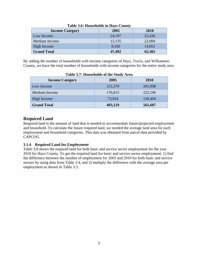
Table 3.6 shows total number of households with income categories in Hays County for 2005 and 2010.

5

Table 3.6: Households in Hays County Income Category 2005 2010

Low Income 24,197 25,430 Medium Income 15,135 22,084 High Income 8,160 14,851 Grand Total 47,492 62,365

By adding the number of households with income categories of Hays, Travis, and Williamson County, we have the total number of households with income categories for the entire study area.

Table 3.7: Households of the Study Area

Income Category 2005 2010

Low Income 232,370 205,998

Medium Income 176,815 225,196

High Income 73,934 130,494

Grand Total 483,119 561,687

Required Land Required land is the amount of land that is needed to accommodate future/projected employment and household. To calculate the future required land, we needed the average land area for each employment and household categories. This data was obtained from parcel data provided by CAPCOG.

3.1.4 Required Land for Employment Table 3.8 shows the required land for both basic and service sector employment for the year 2010 for Hays County. To get the required land for basic and service sector employment: 1) find the difference between the number of employment for 2005 and 2010 for both basic and service sectors by using data from Table 3.4, and 2) multiply the difference with the average area per employment as shown in Table 3.3.

6

Table 3.8: Required Land for Employment in Hays County

Employment Categories Growth 2005-2010 Required Land

(Sq.Ft)

Basic Service Basic Service

Accommodation and Food Services 0 628 0 334,463

Administrative and Support and Waste Management and Remediation Services

0 564 0 745,797

Agriculture, Forestry, Fishing and Hunting 0 0 0 0

Arts, Entertainment, and Recreation 0 111 0 179,990

Construction 258 987 800,673 3,063,549

Educational Services 507 3,789 387,004 2,893,702

Finance and Insurance 0 198 0 247,284

Health Care and Social Assistance 0 315 0 302,081

Information 0 1 0 1,364

Manufacturing 74 170 87,959 194,399

Other Services (except Public Administration) 20 90 41,710 187,227

Professional, Scientific, and Technical Services 0 150 0 219,377

Real Estate and Rental and Leasing 0 28 0 72,177

Retail Trade 202 297 223,750 327,560

Transportation and Warehousing 0 0 0 0

Utilities -7 10 -6,101 8,692

Wholesale Trade 0 17 0 16,173

Table 3.9 shows the total required land for basic and service sector employment of the entire study area. It was obtained by adding required land for basic and service sector employment of Hays, Travis, and Williamson County.

7

Table 3.9: Required Land for Employment in the Study Area Employment Categories Required Land (Sq.Ft)

Basic Service Accommodation and Food Services 266,572 266,448 Administrative and Support and Waste Management and Remediation Services

1,580,969 5,451,375

Agriculture, Forestry, Fishing and Hunting Arts, Entertainment, and Recreation 151,756 1,382,763 Construction 1,473,996 11,229,201 Educational Services 1,735,968 31,467,342 Finance and Insurance 0 1,145,659 Health Care and Social Assistance 0 2,347,173 Information -354,996 237,304 Manufacturing -859,341 841,043 Other Services (except Public Administration) 105,826 990,066 Professional, Scientific, and Technical Services 688,862 1,774,061 Real Estate and Rental and Leasing 0 658,817 Retail Trade 956,184 3,104,811 Transportation and Warehousing 0 56,919 Utilities -7,677 64,662 Wholesale Trade 85,208 308,845 Grand Total 5,823,329 63,726,487

3.1.5 Required Land for Household Based on the result of the regression analysis (for census block groups data of the study area with variables: total number of low income, medium income and high income, sum of area of single family, sum of area of multifamily, and total count of single family), we derived a formula (Table 3.10) to calculate the required land for household. Table 3.11 shows the required land for household of the study area.

Table 3.10: Formula from Regression Analysis Income Category

Area for

=

X Change in Household

Low Income

MF 2021.1 - 9378.4 SF 2234.4

+

11836006.9Medium Income

MF 1221.7 402759.4 SF 31167.2 4828423.1

High Income

MF 888.6 583922.5 SF 45120.5 6300425.4

8

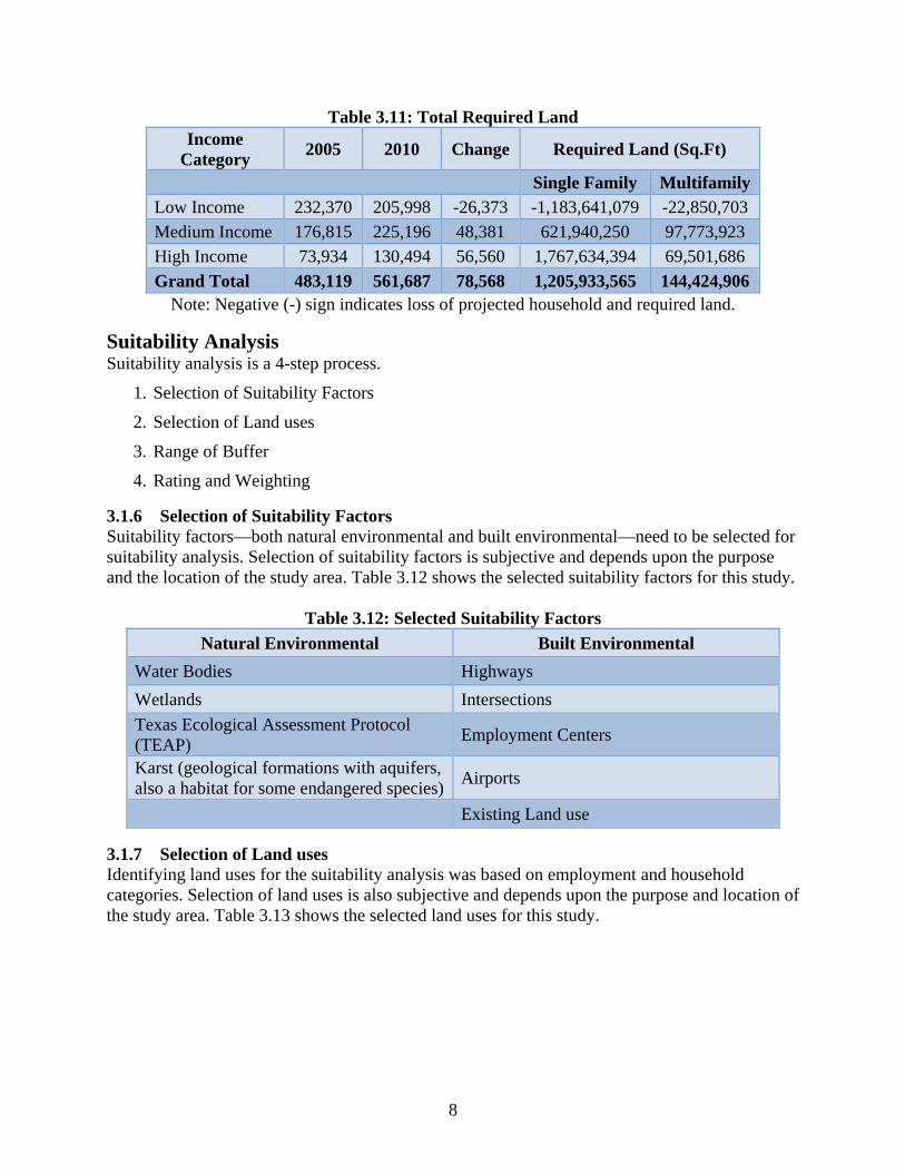
Table 3.11: Total Required Land Income

Category 2005 2010 Change Required Land (Sq.Ft)

Single Family MultifamilyLow Income 232,370 205,998 -26,373 -1,183,641,079 -22,850,703

Medium Income 176,815 225,196 48,381 621,940,250 97,773,923 High Income 73,934 130,494 56,560 1,767,634,394 69,501,686

Grand Total 483,119 561,687 78,568 1,205,933,565 144,424,906 Note: Negative (-) sign indicates loss of projected household and required land.

Suitability Analysis Suitability analysis is a 4-step process.

1. Selection of Suitability Factors

2. Selection of Land uses

3. Range of Buffer

4. Rating and Weighting

3.1.6 Selection of Suitability Factors Suitability factors—both natural environmental and built environmental—need to be selected for suitability analysis. Selection of suitability factors is subjective and depends upon the purpose and the location of the study area. Table 3.12 shows the selected suitability factors for this study.

Table 3.12: Selected Suitability Factors

Natural Environmental Built Environmental

Water Bodies Highways

Wetlands Intersections

Texas Ecological Assessment Protocol (TEAP)

Employment Centers

Karst (geological formations with aquifers, also a habitat for some endangered species)

Airports

Existing Land use

3.1.7 Selection of Land uses Identifying land uses for the suitability analysis was based on employment and household categories. Selection of land uses is also subjective and depends upon the purpose and location of the study area. Table 3.13 shows the selected land uses for this study.

9

Table 3.13: Selected Land Uses Use Categories Activities

Single-Family residential (SF)

Multi-Family residential (MF)

Basic Low Commercial (BLC) Service Low Commercial (SLC)

Offices, assisted living, day care, retail sales and services, restaurants, banks, nursery or greenhouse, grocery sales, pharmacies, fitness centers, dance and music academies, artist studio, colleges and universities, bed and breakfast.

Basic High Commercial (BHC) Service High Commercial (SHC)

Any use in Low Commercial plus bar, nightclub, entertainment venues, hospital, hotel, liquor store, office/warehouse, vehicle and equipment sales, leasing and repair, furniture sales, pet shop, wholesale activities.

Basic Light Industrial (BLI) Service Light Industrial (SLI)

Any use in HC plus commercial laundry, contractor storage yard, lumber yards, indoor manufacture, assembly and processing, mini-warehouse, RV, trailer and boat storage, SOB’s, testing and research, warehouse and distribution, wholesale, wrecker impoundment.

Basic Heavy Industrial (BHI) Service Heavy Industrial (SHI)

Any use in LI plus outdoor manufacture, assembly and processing.

Open Space (OS) City parks, pocket parks , community gardens, outdoor recreational areas, natural areas, environmentally sensitive areas, greenways

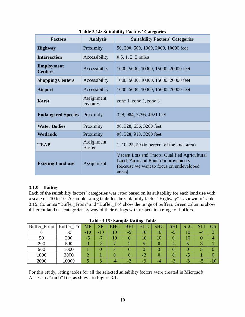
3.1.8 Suitability Factors’ Categories Proximity/accessibility to the suitability factors was used to determine the location of future development. Proximity/accessibility was defined by buffer ranges around each factor. Buffer values are included in the rating table. Table 3.14 shows a range of buffers for the selected suitability factors.

10

Table 3.14: Suitability Factors’ Categories

Factors Analysis Suitability Factors’ Categories

Highway Proximity 50, 200, 500, 1000, 2000, 10000 feet

Intersection Accessibility 0.5, 1, 2, 3 miles

Employment Centers

Accessibility 1000, 5000, 10000, 15000, 20000 feet

Shopping Centers Accessibility 1000, 5000, 10000, 15000, 20000 feet

Airport Accessibility 1000, 5000, 10000, 15000, 20000 feet

Karst Assignment Features

zone 1, zone 2, zone 3

Endangered Species Proximity 328, 984, 2296, 4921 feet

Water Bodies Proximity 98, 328, 656, 3280 feet

Wetlands Proximity 98, 328, 918, 3280 feet

TEAP Assignment Raster

1, 10, 25, 50 (in percent of the total area)

Existing Land use Assignment

Vacant Lots and Tracts, Qualified Agricultural Land, Farm and Ranch Improvements (because we want to focus on undeveloped areas)

3.1.9 Rating Each of the suitability factors’ categories was rated based on its suitability for each land use with a scale of -10 to 10. A sample rating table for the suitability factor “Highway” is shown in Table 3.15. Columns “Buffer_From” and “Buffer_To” show the range of buffers. Green columns show different land use categories by way of their ratings with respect to a range of buffers.

Table 3.15: Sample Rating Table Buffer_From Buffer_To MF SF BHC BHI BLC SHC SHI SLC SLI OS

0 50 -10 -10 10 -5 10 10 -5 10 -4 2 50 200 -5 -7 10 0 10 10 0 10 0 4 200 500 0 -3 7 2 5 8 4 5 3 1 500 1000 1 0 3 6 0 3 6 0 5 0 1000 2000 2 1 0 8 -2 0 8 -5 1 0 2000 10000 5 3 -4 -2 -3 -4 -3 -3 -5 -10

For this study, rating tables for all the selected suitability factors were created in Microsoft Access as “.mdb” file, as shown in Figure 3.1.

11

Figure 3.1: Screenshot of Rating Table in Microsoft Office Access

Note: Any land use that is rated “-11” is considered “null” and masked.

3.1.10 Weighting For calculating each factor’s weight, the AHP model was used. Therefore, all factors were compared with each other in a pair-wise comparison matrix, which is a measure to express the relative preference among the factors. Each factor was weighted expressing a judgment of the relative importance or preference of one factor against other as tabulated in .dbf format (shown in Figure 3.2).

Figure 3.2: Screenshot of the AHP Weighting Table in Microsoft Office Access

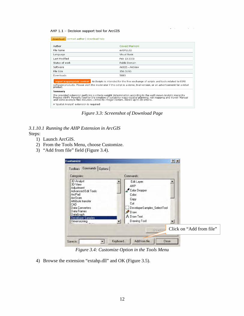
The table was then entered in the AHP Extension to get weighting for all the land uses, as shown in Figure 3.3. AHP Extension can be downloaded from http://arcscripts.esri.com/details.asp?dbid=13764.

12

Figure 3.3: Screenshot of Download Page

3.1.10.1 Running the AHP Extension in ArcGIS Steps:

1) Launch ArcGIS. 2) From the Tools Menu, choose Customize. 3) “Add from file” field (Figure 3.4).

Figure 3.4: Customize Option in the Tools Menu

4) Browse the extension “extahp.dll” and OK (Figure 3.5).

Click on “Add from file”

13

Figure 3.5: Adding the AHP Extension

5) On the Commands tab, choose “Developer Samples” from “Categories.” 6) Choose AHP from the “Commands” list box. 7) Drag AHP onto the ArcMap environment (Figure 3.6).

Figure 3.6: Adding AHP Toolbar

The ArcMap environment looks like this (Figure 3.7):

Figure 3.7: AHP Toolbar

14

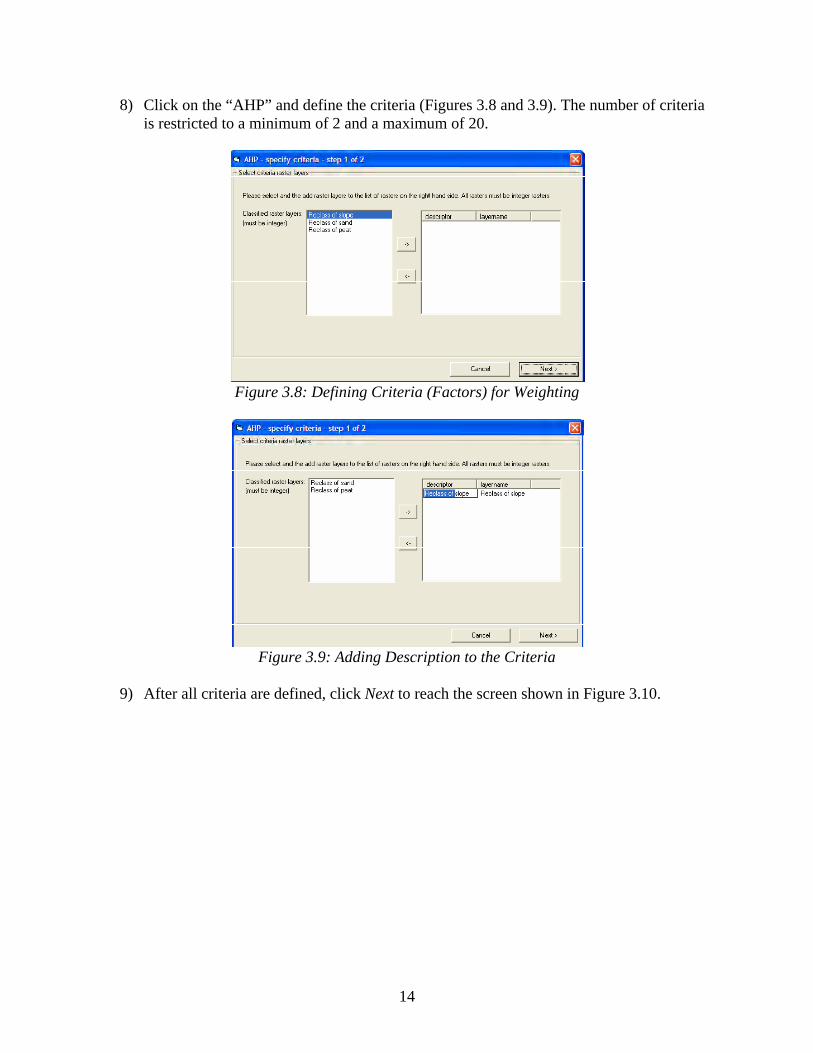
8) Click on the “AHP” and define the criteria (Figures 3.8 and 3.9). The number of criteria is restricted to a minimum of 2 and a maximum of 20.

Figure 3.8: Defining Criteria (Factors) for Weighting

Figure 3.9: Adding Description to the Criteria

9) After all criteria are defined, click Next to reach the screen shown in Figure 3.10.

15

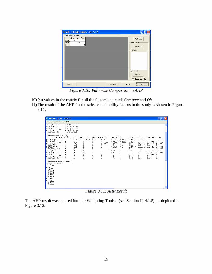
Figure 3.10: Pair-wise Comparison in AHP

10) Put values in the matrix for all the factors and click Compute and Ok. 11) The result of the AHP for the selected suitability factors in the study is shown in Figure

3.11:

Figure 3.11: AHP Result

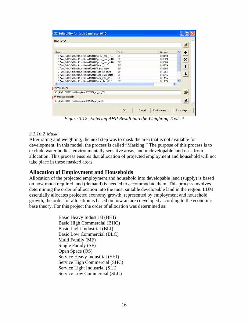
The AHP result was entered into the Weighting Toolset (see Section II, 4.1.5), as depicted in Figure 3.12.

16

Figure 3.12: Entering AHP Result into the Weighting Toolset

3.1.10.2 Mask After rating and weighting, the next step was to mask the area that is not available for development. In this model, the process is called “Masking.” The purpose of this process is to exclude water bodies, environmentally sensitive areas, and undevelopable land uses from allocation. This process ensures that allocation of projected employment and household will not take place in these masked areas.

Allocation of Employment and Households Allocation of the projected employment and household into developable land (supply) is based on how much required land (demand) is needed to accommodate them. This process involves determining the order of allocation into the most suitable developable land in the region. LUM essentially allocates projected economy growth, represented by employment and household growth; the order for allocation is based on how an area developed according to the economic base theory. For this project the order of allocation was determined as:

Basic Heavy Industrial (BHI) Basic High Commercial (BHC) Basic Light Industrial (BLI) Basic Low Commercial (BLC) Multi Family (MF) Single Family (SF) Open Space (OS) Service Heavy Industrial (SHI) Service High Commercial (SHC) Service Light Industrial (SLI) Service Low Commercial (SLC)

17

Section II: Prototype Model and Step-by-Step Process Section II is intended to provide user friendly step-by-step guide to run the SA Model for similar types of applications.

4. Running the SA Model Toolbox in ArcGIS The SA model application in ArcGIS was developed using Model Builder. The following are the steps performed to run the model:

1) Open ArcMap. 2) Open Arc Toolbox and add Toolbox (Figure 4.1).

Figure 4.1: Adding the Model Toolbox

3) Add the SA Model toolbox (Figure 4.2).

Figure 4.2: The Model in ArcToolbox

The prototype model is divided into three toolsets: Rating, Weighting, and Allocation.

2. To add the SA Toolbox, right click and select add toolbox, select from the folder where the SA Model is located.

1. Click to open ArcToolbox

18

Rating Toolset The Rating toolset performs the straight-line distance analysis for the related suitability factors, assigns the rating tables (.mdb), and produces a raster layer, which includes the ratings for each land use in its attribute table.

4.1.1 Proximity SA Model Rating Proximity

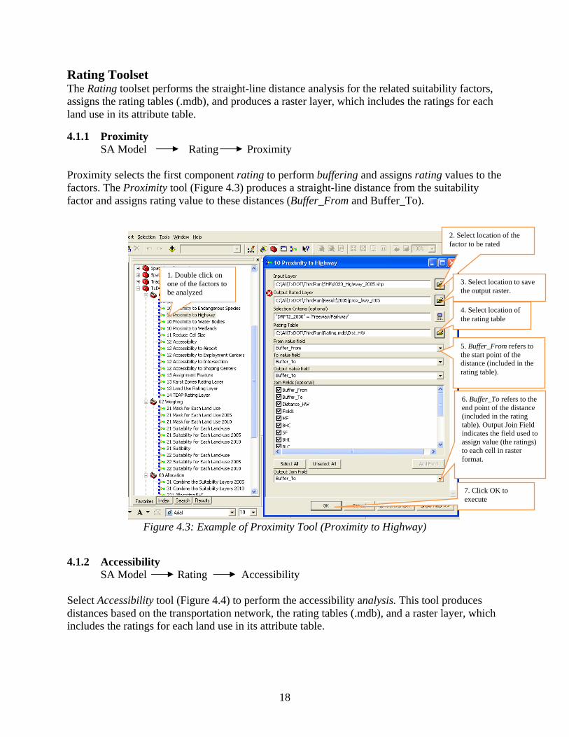
Proximity selects the first component rating to perform buffering and assigns rating values to the factors. The Proximity tool (Figure 4.3) produces a straight-line distance from the suitability factor and assigns rating value to these distances (Buffer_From and Buffer_To).

Figure 4.3: Example of Proximity Tool (Proximity to Highway)

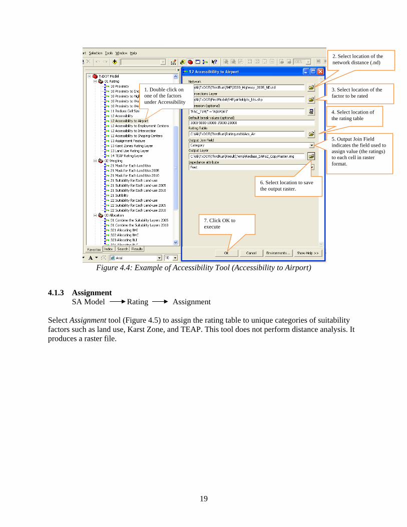
4.1.2 Accessibility SA Model Rating Accessibility

Select Accessibility tool (Figure 4.4) to perform the accessibility analysis. This tool produces distances based on the transportation network, the rating tables (.mdb), and a raster layer, which includes the ratings for each land use in its attribute table.

1. Double click on one of the factors to be analyzed

2. Select location of the factor to be rated

4. Select location of the rating table

7. Click OK to execute

5. Buffer_From refers to the start point of the distance (included in the rating table).

6. Buffer_To refers to the end point of the distance (included in the rating table). Output Join Field indicates the field used to assign value (the ratings) to each cell in raster format.

3. Select location to save the output raster.

19

Figure 4.4: Example of Accessibility Tool (Accessibility to Airport)

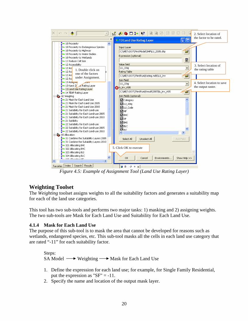
4.1.3 Assignment SA Model Rating Assignment

Select Assignment tool (Figure 4.5) to assign the rating table to unique categories of suitability factors such as land use, Karst Zone, and TEAP. This tool does not perform distance analysis. It produces a raster file.

1. Double click on one of the factors under Accessibility

3. Select location of the factor to be rated



5. Output Join Field indicates the field used to assign value (the ratings) to each cell in raster format.


2. Select location of the network distance (.nd)

20

Figure 4.5: Example of Assignment Tool (Land Use Rating Layer)

Weighting Toolset The Weighting toolset assigns weights to all the suitability factors and generates a suitability map for each of the land use categories. This tool has two sub-tools and performs two major tasks: 1) masking and 2) assigning weights. The two sub-tools are Mask for Each Land Use and Suitability for Each Land Use.

4.1.4 Mask for Each Land Use The purpose of this sub-tool is to mask the area that cannot be developed for reasons such as wetlands, endangered species, etc. This sub-tool masks all the cells in each land use category that are rated “-11” for each suitability factor.

Steps: SA Model Weighting Mask for Each Land Use 1. Define the expression for each land use; for example, for Single Family Residential,

put the expression as "SF" = -11. 2. Specify the name and location of the output mask layer.

1. Double click on one of the factors under Assignment.

2. Select location of the factor to be rated.




21

3. Put raster datasets of all the selected suitability factors from the database. For example, for wetlands, put the raster file “prox_wet_rt10.”

4. Click OK.

Similarly, we can perform masking for other land use categories, as shown in Figure 4.6.

Figure 4.6: Mask Tool for Each Land Use

Result: The white areas of the map are masked for Single Family (SF) development (Figure 4.7). This means SF development cannot be allocated in these areas.

Figure 4.7: Result of the Mask Tool

4.1.5 Suitability for Each Land Use This component of the Weighting tool uses AHP results (weight scores) for each land use to get the suitability layers.

22

Steps: SA Model Weighting Suitability for Each Land Use

1. Put raster files of all the suitability factors in the “input layer.” 2. Select the land use under “Field;” here the selected land use is SF. 3. Use the weights that are generated by AHP (refer to section 2.3.5.1). 4. Specify the name and location of the “Output Layer.” 5. Put the mask layer. For example, here the mask layer for SF is “sf_mask” (as

shown in Figure 4.8). 6. Click OK.

Figure 4.8: Suitability for Each Land Use Tool

Allocation Toolset The Allocation toolset combines the entire suitability map for all land use categories, allocates each land use into the most suitable location, and produces the composite allocation map. This tool has three sub-tools.

4.1.6 Combine the Suitability Layers Select the Combine the Suitability Layers 2010 to combine the entire suitability layers of each land use. This tool creates one composite raster layer that has the values of each land use in different fields in its attribute table.

Steps: SA Model Allocation Combine the Suitability Layers 2010

23

Figure 4.9: Combine the Suitability Layers Tool

4.1.7 Allocating The Allocating toolset is used to allocate the required land (from section 2.2) on suitable land for each land use.

Steps: SA Model Allocation Allocating

Currently, the value of required land is set based on 2010 household and employment projections. However, this value can be adjusted for running different scenarios for employment and population growth.

1. Select Allocation 2. Double click on Combine the Suitability Layer


4. Select location where the individual suitability map was saved.


24

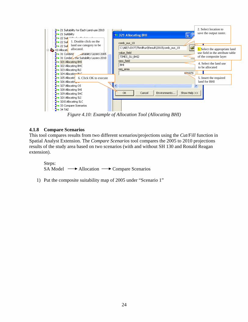
Figure 4.10: Example of Allocation Tool (Allocating BHI)

4.1.8 Compare Scenarios This tool compares results from two different scenarios/projections using the Cut/Fill function in Spatial Analyst Extension. The Compare Scenarios tool compares the 2005 to 2010 projections results of the study area based on two scenarios (with and without SH 130 and Ronald Reagan extension).

Steps: SA Model Allocation Compare Scenarios

1) Put the composite suitability map of 2005 under “Scenario 1”

1. Double click on the land use category to be allocated.


3. Select the appropriate land use field in the attribute table of the composite layer

5. Insert the required land for BHI

4. Select the land use to be allocated


25

Figure 4.11: Adding Scenario 1 Result in Compare Scenarios Tool

2) Select the land use type of interest under “Base Field 1).” 3) Put the composite suitability map of 2010 under “Scenario 2.”

Figure 4.12: Adding Scenario 2 Result in Compare Scenario Tool

26

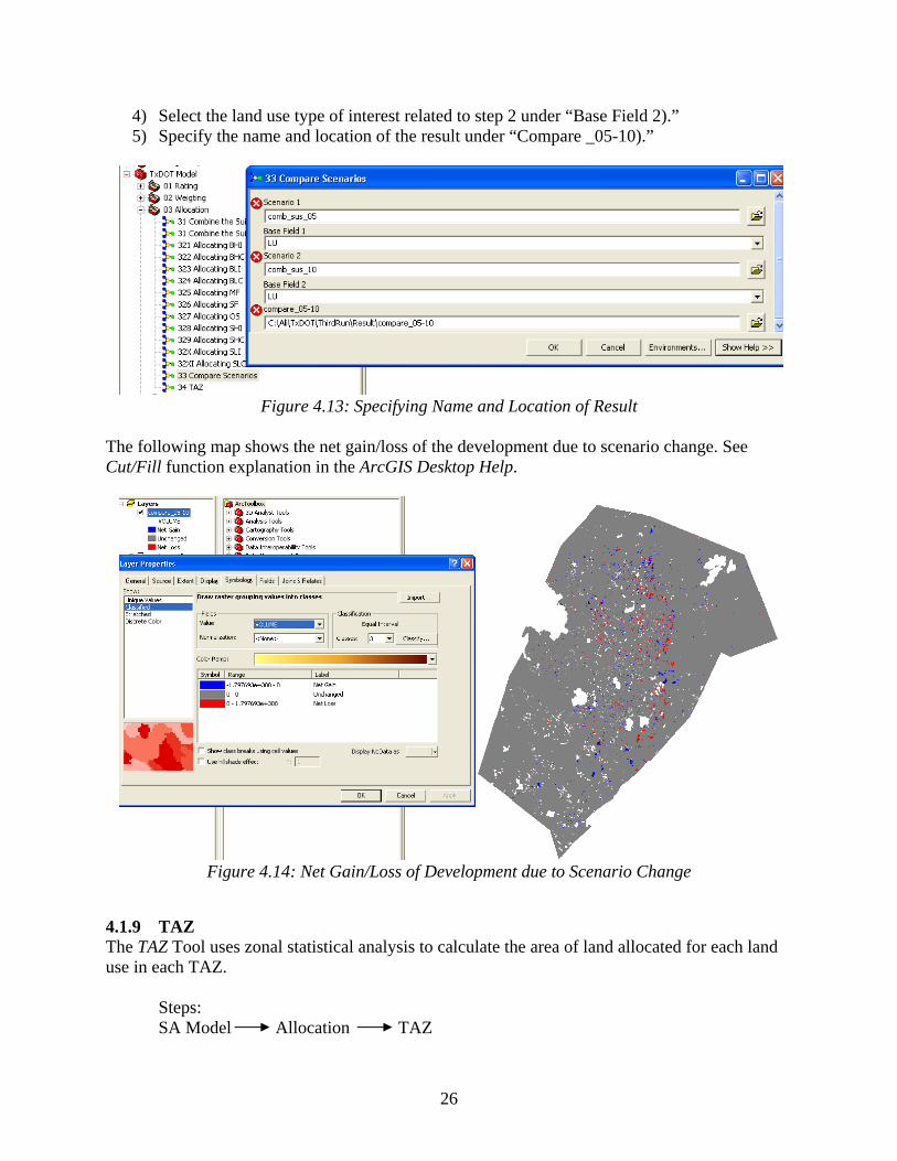
4) Select the land use type of interest related to step 2 under “Base Field 2).” 5) Specify the name and location of the result under “Compare _05-10).”

Figure 4.13: Specifying Name and Location of Result

The following map shows the net gain/loss of the development due to scenario change. See Cut/Fill function explanation in the ArcGIS Desktop Help.

Figure 4.14: Net Gain/Loss of Development due to Scenario Change

4.1.9 TAZ The TAZ Tool uses zonal statistical analysis to calculate the area of land allocated for each land use in each TAZ.

Steps: SA Model Allocation TAZ

27

Figure 4.15: TAZ Tool

This step should be repeated for each land use. The result is a TAZ shapefile that contains allocated land for all the land uses. To obtain employment and household density in TAZ, follow the steps below: 1) Open the attribute table of TAZ shape file and copy it to Excel.

Figure 4.16: TAZ Attribute Field

2. Double-click on TAZ

1. Select Allocation

3. Select the location of the final composite map

4. Specify the land use field to calculate its area in each TAZ

Select location to save the output

28

Figure 4.17: Select all the Fields in the Attribute Table and Copy to Microsoft Excel

2) Get the average square feet of land per employment and the average square feet of land per

single family and multifamily household (this can be obtained from the existing average square feet per employment under the assumption that the region will continue to grow the same way. There are also other resources that may provide standard calculation of average area per employee.)

3) In Microsoft Excel, calculate total number of employment. For basic employment, divide the sum of the allocated land for basic employment by the average square feet of land per employment. For service employment, divide the sum of the allocated land for service employment by the average feet of land per employment.

4) Calculate the total number of households. For single family household, divide the total allocated land for single family by the average square feet of land per single family household. Similarly, for multifamily, divide the total allocated land for multifamily by the average square feet of land per multifamily.

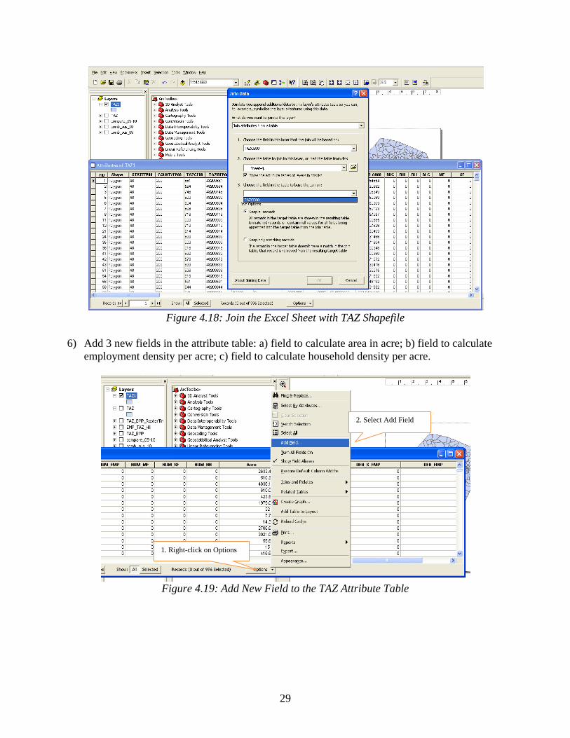
5) Join the newly created Excel spreadsheet with the TAZ shape file.

29

Figure 4.18: Join the Excel Sheet with TAZ Shapefile

6) Add 3 new fields in the attribute table: a) field to calculate area in acre; b) field to calculate

employment density per acre; c) field to calculate household density per acre.

Figure 4.19: Add New Field to the TAZ Attribute Table

1. Right-click on Options

2. Select Add Field

30

Figure 4.20: Calculate Area in Acre

Figure 4.21: Calculate Employment Density in Field Calculator

1. Right-click on the field

2. Select Calculate Geometry

31

Appendix A: Proximity Tool

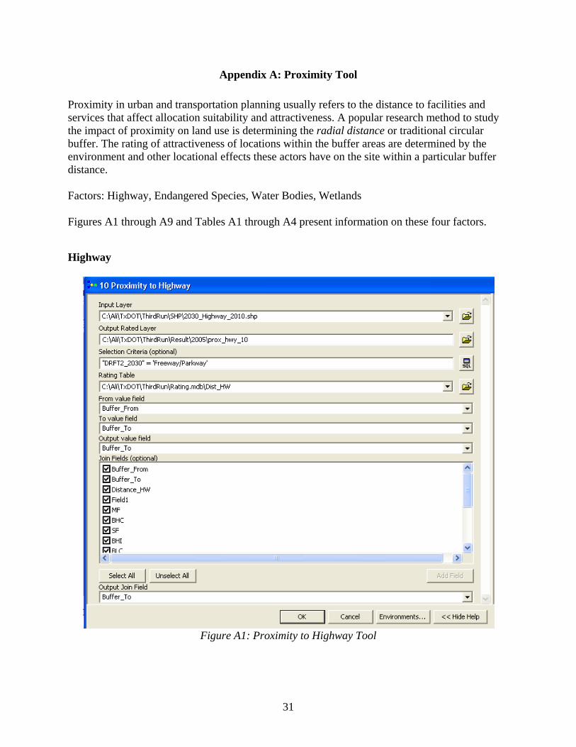
Proximity in urban and transportation planning usually refers to the distance to facilities and services that affect allocation suitability and attractiveness. A popular research method to study the impact of proximity on land use is determining the radial distance or traditional circular buffer. The rating of attractiveness of locations within the buffer areas are determined by the environment and other locational effects these actors have on the site within a particular buffer distance. Factors: Highway, Endangered Species, Water Bodies, Wetlands Figures A1 through A9 and Tables A1 through A4 present information on these four factors.

Highway

Figure A1: Proximity to Highway Tool

32

Input Layer: Select the highway shape file (2030_Highway_2010.shp) Output Rated Layer: Choose the location and name of the output file Selection Criteria: "DRFT2_2030" = 'Freeway/Parkway' OR "DRFT2_2030" = 'Major Arterial' (these are the major highways and roads in the study area) Rating Table: A rating table for highway in mdb format From Value Field: It is the minimum value for buffer, so select "Buffer From.” For Example, the model would consider 0 as the minimum value for highway distance of 0 to 50 feet from the land use type. To Value Field: It is the maximum value for buffer, so select "Buffer To.” For example, the model would consider 50 as the maximum value for highway distance of 0 to 50 feet from the land use type. Output value field: Select “Buffer_to” Join Fields (optional): It is optional but if needed you can select all or some of the fields to show them in the attribute table. Output Join Field: Join the rating table with the result of the analysis to get the output. Here “Distance_HW” is a common field to join the rating table and the result of the analysis.

Table A1: Rating Table for Proximity to Highway

ID Buffer_From Buffer_To Distance_HW Field1 MF BHC SF BHI BLC BLI SHC SHI SLC SLI OS

1 0 50 50 50 -10 10 -10 -5 10 -4 10 -5 10 -4 2

2 50 200 200 200 -5 10 -7 0 10 0 10 0 10 0 4

3 200 500 500 500 0 7 -3 2 5 3 8 4 5 3 1

4 500 1000 1000 1000 1 3 0 6 0 5 3 6 0 5 0

5 1000 2000 2000 2000 2 0 1 8 -2 -1 0 8 -5 -1 0

6 2000 10000 10000 10000 5 -4 3 -2 -3 -5 -4 -3 -3 -5 -10

Figure A2: Result of Proximity to Highway Tool

33

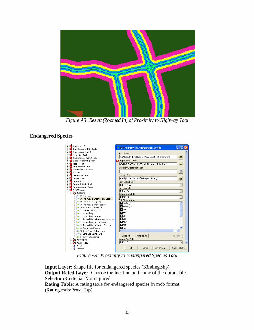
Figure A3: Result (Zoomed In) of Proximity to Highway Tool

Endangered Species

Figure A4: Proximity to Endangered Species Tool

Input Layer: Shape file for endangered species (33nding.shp) Output Rated Layer: Choose the location and name of the output file Selection Criteria: Not required Rating Table: A rating table for endangered species in mdb format (Rating.mdb\Prox_Esp)

34

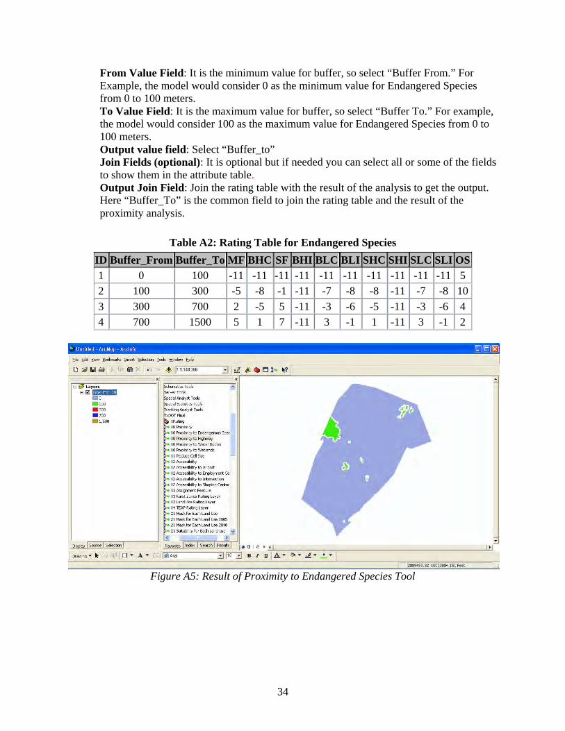
From Value Field: It is the minimum value for buffer, so select “Buffer From.” For Example, the model would consider 0 as the minimum value for Endangered Species from 0 to 100 meters. To Value Field: It is the maximum value for buffer, so select “Buffer To.” For example, the model would consider 100 as the maximum value for Endangered Species from 0 to 100 meters. Output value field: Select “Buffer_to” Join Fields (optional): It is optional but if needed you can select all or some of the fields to show them in the attribute table. Output Join Field: Join the rating table with the result of the analysis to get the output. Here “Buffer_To” is the common field to join the rating table and the result of the proximity analysis.

Table A2: Rating Table for Endangered Species

ID Buffer_From Buffer_To MF BHC SF BHI BLC BLI SHC SHI SLC SLI OS

1 0 100 -11 -11 -11 -11 -11 -11 -11 -11 -11 -11 5

2 100 300 -5 -8 -1 -11 -7 -8 -8 -11 -7 -8 10

3 300 700 2 -5 5 -11 -3 -6 -5 -11 -3 -6 4

4 700 1500 5 1 7 -11 3 -1 1 -11 3 -1 2

Figure A5: Result of Proximity to Endangered Species Tool

35

Water Bodies

Figure A6: Proximity to Water Bodies Tool

Input Layer: Select the shape file for water bodies (SAhydrogena.shp) Output Rated Layer: Choose the location and name of the output file Selection Criteria: “TYPE” = ‘Major Stream’ OR “TYPE” = ‘Major River’ OR “TYPE” = ‘Stream, Water Body’ OR “TYPE” = ‘Water Body’ Rating Table: A rating table for water bodies in mdb format (Rating.mdb\Prox_Wat) From Value Field: It is the minimum value for buffer, so select “Buffer From.” For Example, the model would consider 0 as the minimum value for water bodies from 0 to 30 meters. To Value Field: It is the maximum value for buffer, so select “Buffer To.” For example, the model would consider 30 as the maximum value for water bodies from 0 to 30 meters. Output value field: Select “Buffer_to” Join Fields (optional): It is optional but if needed you can select all or some of the fields to show them in the attribute table. Output Join Field: Join the rating table with the result of the analysis to get the output. Here “Buffer_To” is the common field to join the rating table and the result of the analysis.

36

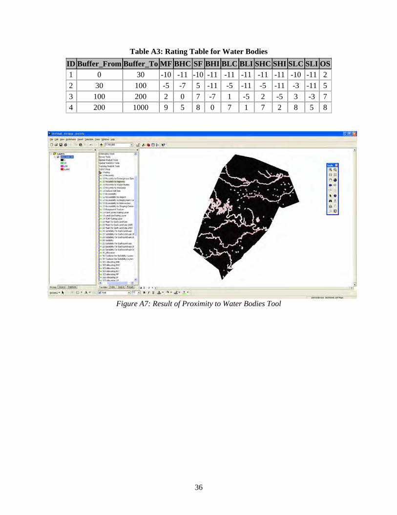
Table A3: Rating Table for Water Bodies


1 0 30 -10 -11 -10 -11 -11 -11 -11 -11 -10 -11 2

2 30 100 -5 -7 5 -11 -5 -11 -5 -11 -3 -11 5

3 100 200 2 0 7 -7 1 -5 2 -5 3 -3 7

4 200 1000 9 5 8 0 7 1 7 2 8 5 8

Figure A7: Result of Proximity to Water Bodies Tool

37

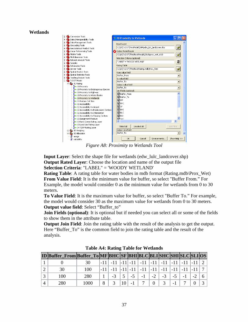
Wetlands

Figure A8: Proximity to Wetlands Tool

Input Layer: Select the shape file for wetlands (edw_lulc_landcover.shp) Output Rated Layer: Choose the location and name of the output file Selection Criteria: "LABEL" = 'WOODY WETLAND' Rating Table: A rating table for water bodies in mdb format (Rating.mdb\Prox_Wet) From Value Field: It is the minimum value for buffer, so select "Buffer From.” For Example, the model would consider 0 as the minimum value for wetlands from 0 to 30 meters. To Value Field: It is the maximum value for buffer, so select "Buffer To.” For example, the model would consider 30 as the maximum value for wetlands from 0 to 30 meters. Output value field: Select “Buffer_to” Join Fields (optional): It is optional but if needed you can select all or some of the fields to show them in the attribute table. Output Join Field: Join the rating table with the result of the analysis to get the output. Here “Buffer_To” is the common field to join the rating table and the result of the analysis.

Table A4: Rating Table for Wetlands


1 0 30 -11 -11 -11 -11 -11 -11 -11 -11 -11 -11 2

2 30 100 -11 -11 -11 -11 -11 -11 -11 -11 -11 -11 7

3 100 280 1 -3 5 -5 -1 -2 -3 -5 -1 -2 6

4 280 1000 8 3 10 -1 7 0 3 -1 7 0 3

38

Figure A9: Result of Proximity to Wetland Tool

39

Appendix B: Accessibility Tool

Factors: Airport, Employment Centers, Intersection, Shopping Centers Figures B1 through B8 and Tables B1 through B4 present information about these four factors.

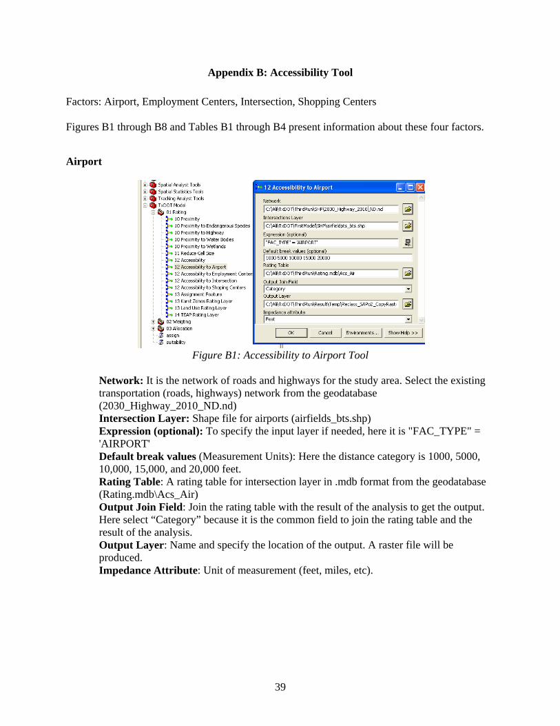
Airport

Figure B1: Accessibility to Airport Tool

Network: It is the network of roads and highways for the study area. Select the existing transportation (roads, highways) network from the geodatabase (2030_Highway_2010_ND.nd) Intersection Layer: Shape file for airports (airfields_bts.shp) Expression (optional): To specify the input layer if needed, here it is "FAC_TYPE" = 'AIRPORT' Default break values (Measurement Units): Here the distance category is 1000, 5000, 10,000, 15,000, and 20,000 feet. Rating Table: A rating table for intersection layer in .mdb format from the geodatabase (Rating.mdb\Acs_Air) Output Join Field: Join the rating table with the result of the analysis to get the output. Here select “Category” because it is the common field to join the rating table and the result of the analysis. Output Layer: Name and specify the location of the output. A raster file will be produced. Impedance Attribute: Unit of measurement (feet, miles, etc).

40

Table B1: Rating Table for Airport

ID Category MF BHC SF BHI BLC BLI SHC SHI SLC SLI OS

1 1000 -10 -5 -10 -3 -4 -5 -5 -10 -5 -10 0

2 5000 -5 -3 -7 -1 -2 -4 -3 -9 -2 -9 1

3 10000 0 0 0 1 2 -3 0 -8 0 -8 4

4 15000 2 1 1 2 4 0 1 0 4 0 5

5 20000 3 2 5 -1 6 3 2 0 6 2 7

Figure B2: Result of Accessibility to Airport Tool

Employment Centers

Figure B3: Accessibility to Employment Centers Tool

41

Network: Select the existing transportation (roads, highways) network from the geodatabase (2030_Highway_2010_ND.nd) Intersection Layer: Shape file for employment centers (emp_cntr.shp) Expression (optional): To specify the input layer if needed, here it is "NUMBER_EMP" >100 Default break values (Measurement Units): Here the distance category is 1000, 5000, 10,000, 15,000, and 20,000 feet. Rating Table: Rating table for intersection layer in .mdb format from the geodatabase (Rating.mdb\Acs_Emp) Output Join Field: Join the rating table with the result of the analysis to get the output. Here select “Category” is the common field to join the rating table and the result of the analysis. Output Layer: Specify the location and name of the output. A raster file will be produced. Impedance Attribute: Unit of measurement (feet, miles, etc).

Table B2: Rating Table for Employment Centers


1 1000 -10 7 -10 -10 10 -10 7 -10 10 -10 0

2 5000 0 8 -2 -7 8 -5 8 -7 8 -5 2

3 10000 3 6 1 -3 5 -1 6 -3 5 -1 4

4 15000 2 1 3 -1 0 0 1 -1 0 0 -1

5 20000 -1 0 -5 0 -1 1 0 0 -1 1 -5

Figure B4: Result of Accessibility to Employment Centers Tool

42

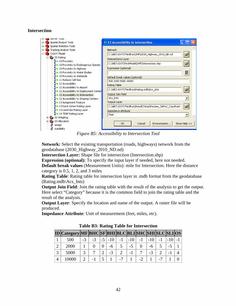
Intersection

Figure B5: Accessibility to Intersection Tool

Network: Select the existing transportation (roads, highways) network from the geodatabase (2030_Highway_2010_ND.nd) Intersection Layer: Shape file for intersection (Intersection.shp) Expression (optional): To specify the input layer if needed, here not needed. Default break values (Measurement Units): mile for Intersection. Here the distance category is 0.5, 1, 2, and 3 miles Rating Table: Rating table for intersection layer in .mdb format from the geodatabase (Rating.mdb\Acs_Ints) Output Join Field: Join the rating table with the result of the analysis to get the output. Here select “Category” because it is the common field to join the rating table and the result of the analysis. Output Layer: Specify the location and name of the output. A raster file will be produced. Impedance Attribute: Unit of measurement (feet, miles, etc).

Table B3: Rating Table for Intersection


1 500 -3 -3 -5 -10 -1 -10 -1 -10 -1 -10 -1

2 2000 1 0 0 -6 5 -5 0 -6 5 -5 1

3 5000 3 7 2 -3 2 -1 7 -3 2 -1 4

4 10000 2 -1 5 1 -7 1 -2 1 -7 1 0

43

Figure B6: Result of Accessibility to Intersection Tool

Shopping Centers

Figure B7: Accessibility to Shopping Centers Tool

Network: Select the existing transportation (roads, highways) network from the geodatabase (2030_Highway_2010_ND.nd) Intersection Layer: Shape file for shopping centers (shp_cntr.shp) Expression (optional): To specify the input layer if needed, here it is not needed. Default break values (Measurement Units): Here the distance category is 1000, 5000, 10,000, 15,000, and 20,000 feet. Rating Table: Rating table for intersection layer in .mdb format from the geodatabase (Rating.mdb\Acs_Shp)

44

Output Join Field: Join the rating table with the result of the analysis to get the output. Here select “Category” t is the common field to join the rating table and the result of the analysis. Output Layer: Specify the location and name of the output. A raster file will be produced. Impedance Attribute: Unit of measurement (feet, miles, etc).

Table B4: Rating Table for Shopping Centers


1 1000 -10 7 -10 -10 10 -10 7 -10 10 -10 0

2 5000 0 8 0 -7 8 -5 8 -7 8 -5 3

3 10000 3 6 1 -3 7 -1 6 -3 5 -1 5

4 15000 0 1 0 -1 0 0 1 -1 0 0 0

5 20000 -6 0 -5 0 -1 1 0 0 -2 1 -3

Figure B8: Result of Accessibility to Shopping Centers Tool

45

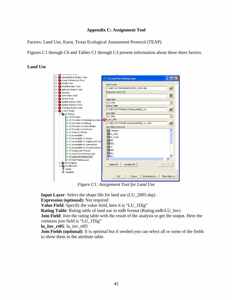
Appendix C: Assignment Tool

Factors: Land Use, Karst, Texas Ecological Assessment Protocol (TEAP) Figures C1 through C6 and Tables C1 through C3 present information about these three factors.

Land Use

Figure C1: Assignment Tool for Land Use

Input Layer: Select the shape file for land use (LU_2005.shp) Expression (optional): Not required Value Field: Specify the value field, here it is “LU_1Dig” Rating Table: Rating table of land use in mdb format (Rating.mdb\LU_Inv) Join Field: Join the rating table with the result of the analysis to get the output. Here the common join field is “LU_1Dig” lu_Inv_rt05: lu_inv_rt05 Join Fields (optional): It is optional but if needed you can select all or some of the fields to show them in the attribute table.

46

Table C1: Rating Table for Existing Land Use

ID LU_Code Category MF BHC SF BHI BLC BLI SHC SHI SLC SLI LU_1Dig OS

1 A Single Family Residential

-11 -11 -11

-11 -11 -11 -11 -11 -11 -11 1 -11

2 B Multifamily Residential

-11 -11 -11

-11 -11 -11 -11 -11 -11 -11 2 -11

3 C Vacant Lots and Tracts

10 10 10 10 10 10 10 10 10 10 3 10

4 D Qualified Agricultural

Land

0 -5 5 -5 -5 -5 -5 -7 -2 -5 4 10

5 E Farm and Ranch Improvements

0 -5 5 -5 -5 -5 -5 -7 -2 -5 5 10

6 F Commercial -11 -11 -11

-11 -11 -11 -11 -11 -11 -11 6 -11

7 G Oil, Gas, and Other Minerals

-11 -11 -11

-11 -11 -11 -11 -11 -11 -11 7 -11

8 H Non business vehicles _tangible

personal property

-11 -11 -11

-11 -11 -11 -11 -11 -11 -11 8 -11

9 J Utilities -11 -11 -11

-11 -11 -11 -11 -11 -11 -11 9 -11

10 M Mobile Homes 0 0 1 0 0 0 0 0 0 0 10 0

Figure C2: Result of Assignment of Land Use Tool

47

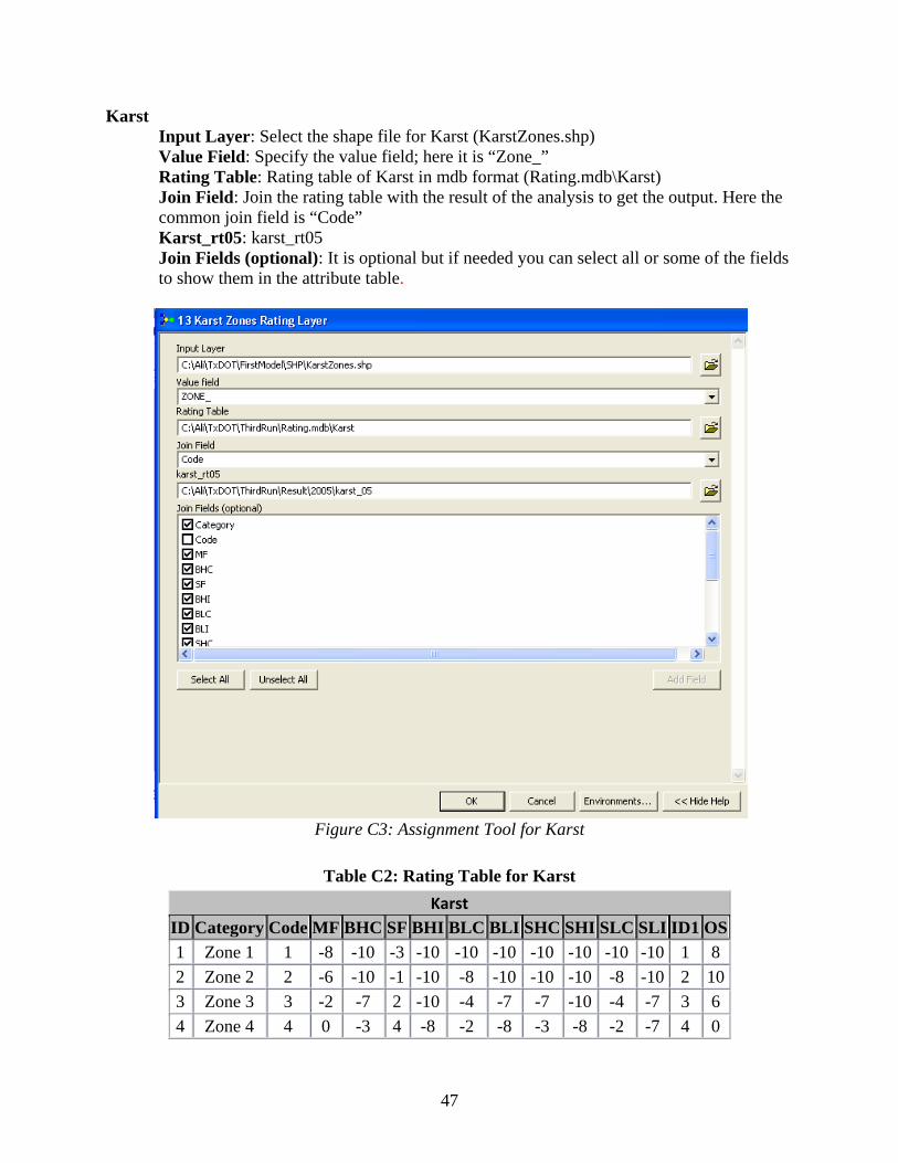
Karst Input Layer: Select the shape file for Karst (KarstZones.shp) Value Field: Specify the value field; here it is “Zone_” Rating Table: Rating table of Karst in mdb format (Rating.mdb\Karst) Join Field: Join the rating table with the result of the analysis to get the output. Here the common join field is “Code” Karst_rt05: karst_rt05 Join Fields (optional): It is optional but if needed you can select all or some of the fields to show them in the attribute table.

Figure C3: Assignment Tool for Karst

Table C2: Rating Table for Karst

Karst ID Category Code MF BHC SF BHI BLC BLI SHC SHI SLC SLI ID1 OS

1 Zone 1 1 -8 -10 -3 -10 -10 -10 -10 -10 -10 -10 1 8

2 Zone 2 2 -6 -10 -1 -10 -8 -10 -10 -10 -8 -10 2 10

3 Zone 3 3 -2 -7 2 -10 -4 -7 -7 -10 -4 -7 3 6

4 Zone 4 4 0 -3 4 -8 -2 -8 -3 -8 -2 -7 4 0

48

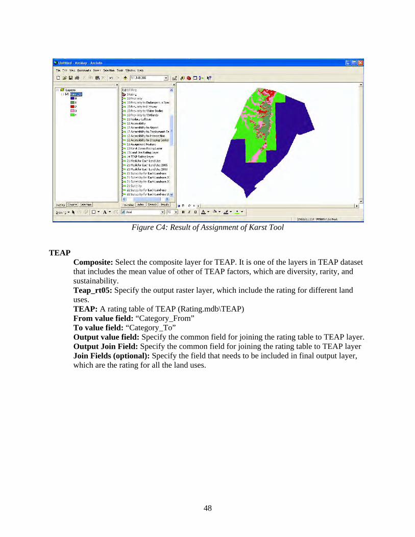
Figure C4: Result of Assignment of Karst Tool

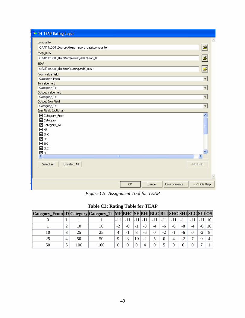
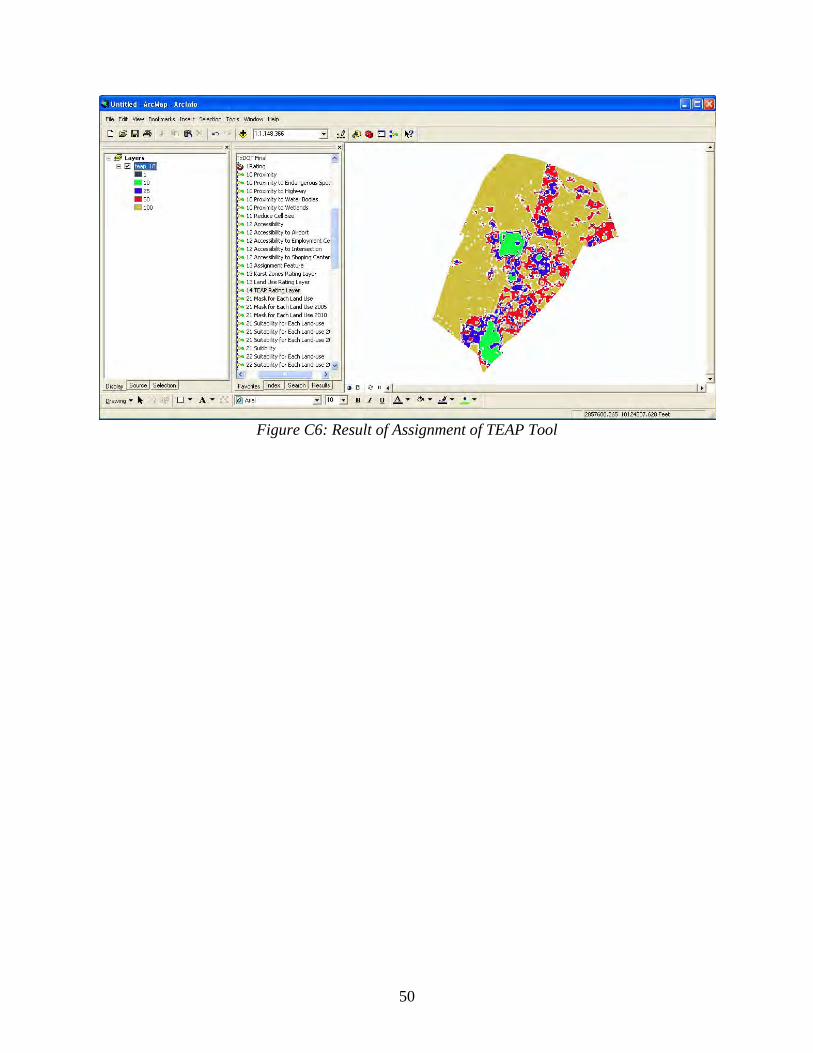
TEAP Composite: Select the composite layer for TEAP. It is one of the layers in TEAP dataset that includes the mean value of other of TEAP factors, which are diversity, rarity, and sustainability. Teap_rt05: Specify the output raster layer, which include the rating for different land uses. TEAP: A rating table of TEAP (Rating.mdb\TEAP) From value field: “Category_From” To value field: “Category_To” Output value field: Specify the common field for joining the rating table to TEAP layer. Output Join Field: Specify the common field for joining the rating table to TEAP layer Join Fields (optional): Specify the field that needs to be included in final output layer, which are the rating for all the land uses.

49

Figure C5: Assignment Tool for TEAP

Table C3: Rating Table for TEAP

Category_From ID Category Category_To MF BHC SF BHI BLC BLI SHC SHI SLC SLI OS

0 1 1 1 -11 -11 -11 -11 -11 -11 -11 -11 -11 -11 10

1 2 10 10 -2 -6 -1 -8 -4 -6 -6 -8 -4 -6 10

10 3 25 25 4 -1 8 -6 0 -2 -1 -6 0 -2 8

25 4 50 50 9 3 10 -2 5 0 4 -2 7 0 4

50 5 100 100 0 0 0 4 0 5 0 6 0 7 1

50

Figure C6: Result of Assignment of TEAP Tool

51

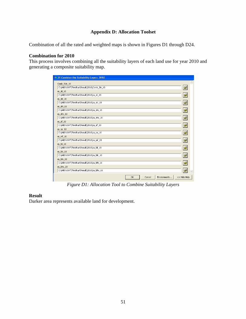
Appendix D: Allocation Toolset

Combination of all the rated and weighted maps is shown in Figures D1 through D24. Combination for 2010 This process involves combining all the suitability layers of each land use for year 2010 and generating a composite suitability map.

Figure D1: Allocation Tool to Combine Suitability Layers

Result Darker area represents available land for development.

52

Figure D2: Result of Allocation Tool Showing Available Land for Development

53

Open Space

Figure D3: Allocation Tool for Open Space

Figure D4: Allocated Open Space

54

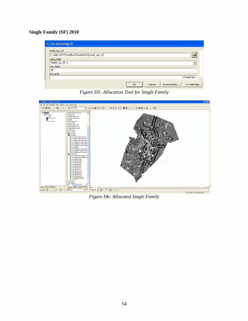
Single Family (SF) 2010

Figure D5: Allocation Tool for Single Family

Figure D6: Allocated Single Family

55

Multi Family (MF)

Figure D7: Allocation Tool for Multi Family

Figure D8: Allocated Multi Family

56

Basic Heavy Industrial (BHI)

Figure D9: Allocation Tool for Basic Heavy Industrial

Figure D10: Allocated Basic Heavy Industrial

57

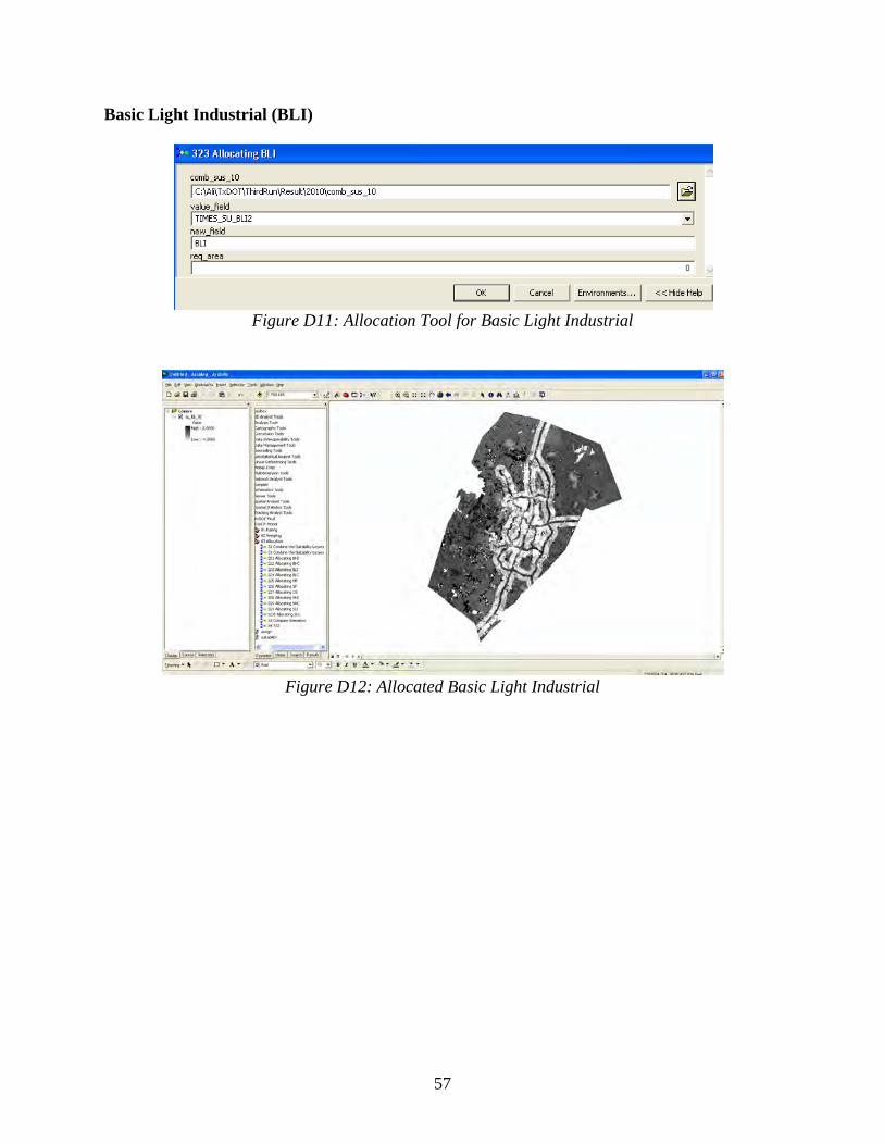
Basic Light Industrial (BLI)

Figure D11: Allocation Tool for Basic Light Industrial

Figure D12: Allocated Basic Light Industrial

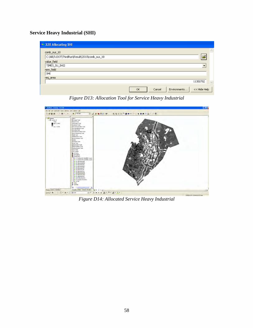
58

Service Heavy Industrial (SHI)

Figure D13: Allocation Tool for Service Heavy Industrial

Figure D14: Allocated Service Heavy Industrial

59

Service Light Industrial (SLI)

Figure D15: Allocation Tool for Service Light Industrial

Figure D16: Allocated Service Light Industrial

60

Basic High Commercial (BHC)

Figure D17: Allocation Tool for Basic High Commercial

Figure D18: Allocated Basic High Commercial

61

Basic Low Commercial (BLC)

Figure D19: Allocation Tool for Basic Low Commercial

Figure D20: Allocated Basic Low Commercial

62

Service High Commercial (SHC)

Figure D21: Allocation Tool for Service High Commercial

Figure D22: Allocated Service High Commercial

63

Service Low Commercial

Figure D23: Allocation Tool for Service Low Commercial

Figure D24: Allocated Service Low Commercial

65

Appendix E: Suitability Tool

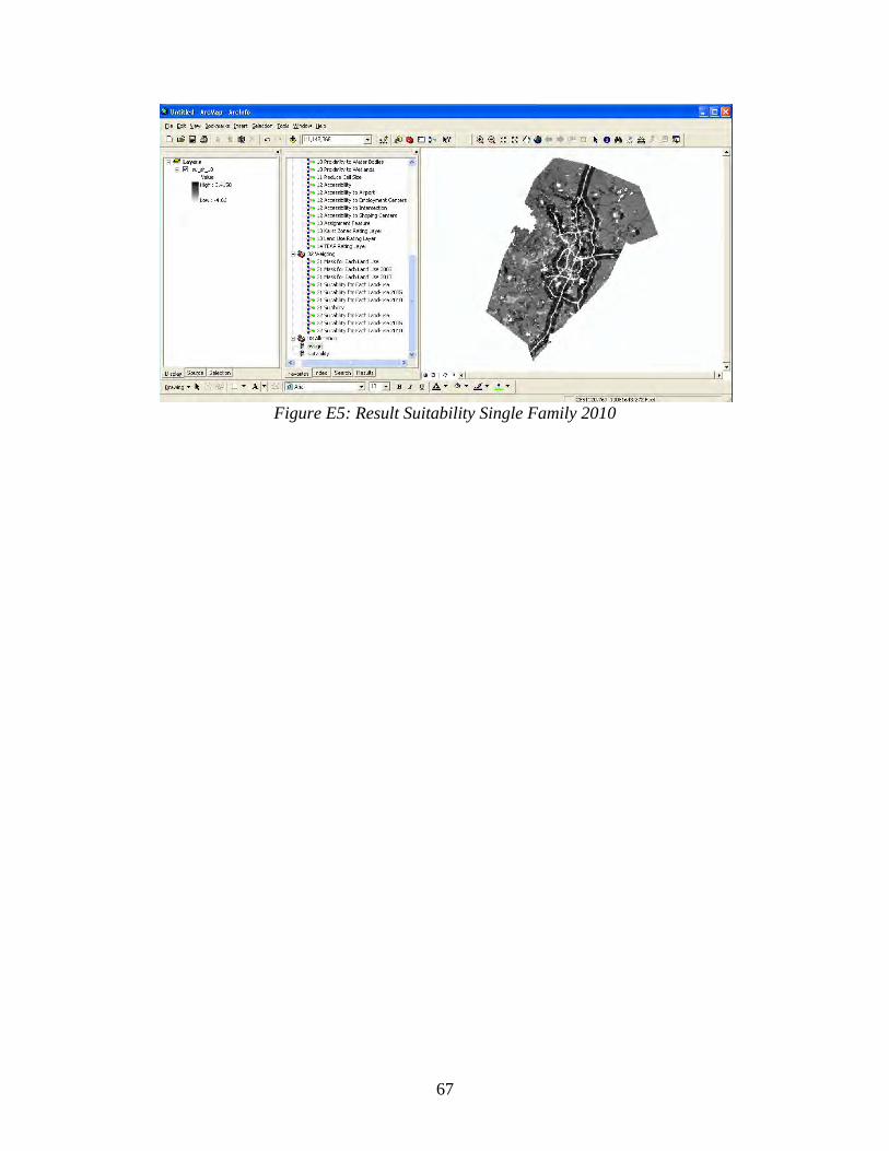
After we get total land available for development, we perform suitability analysis for each land use based on the weight. See Figures E1 through E5.

Figure E1: Suitability Tool

Suitability for 2005 Here, a raster file of each suitability factor for Single Family (SF) land use with assigned weight is entered.

Figure E2: Suitability Tool for 2005

66

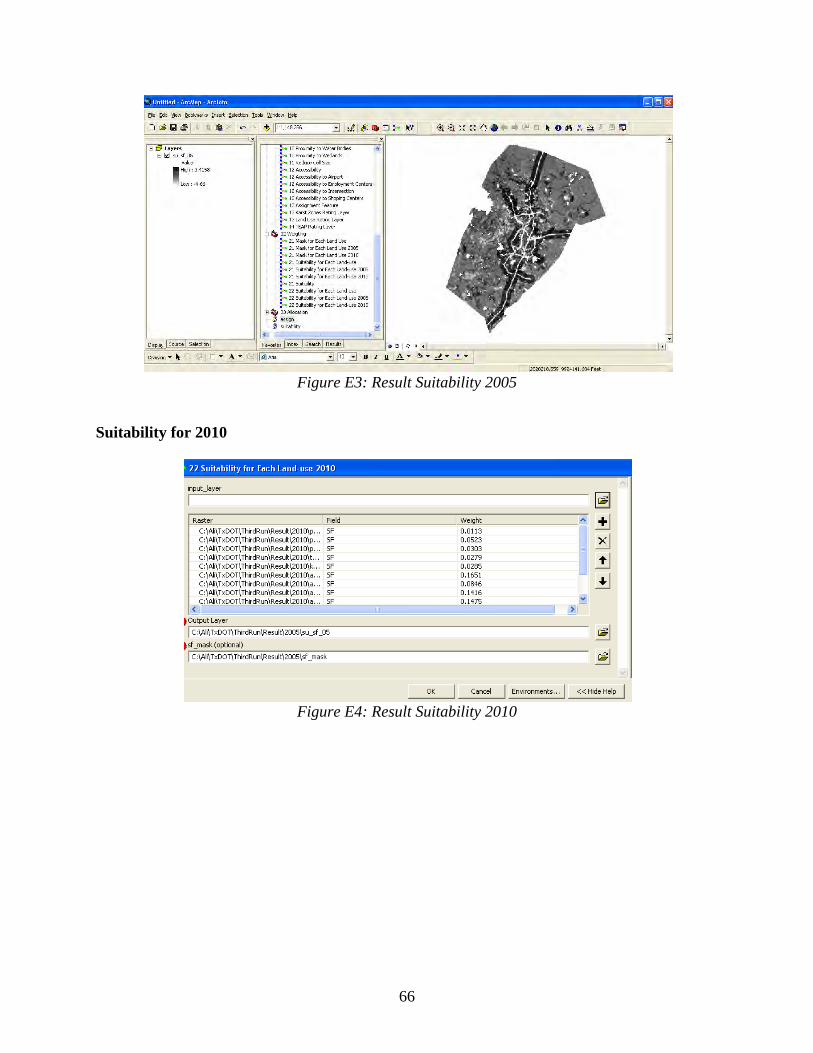
Figure E3: Result Suitability 2005

Suitability for 2010

Figure E4: Result Suitability 2010

67

Figure E5: Result Suitability Single Family 2010

Suitability Analysis Guidebook/Training Materials : Manual...

Documents

Transcript of Suitability Analysis Guidebook/Training Materials : Manual...