f o o t e r - a u t h o r ’ s l a s t n a m e - 7

W i n t e r 2 0 0 9

Subsurface Mapping:

A Question of Position and Interpretation

Andrew C. KellieMurray State University

Abstract

This paper discusses the character and challenges inherent in the graphical portrayal of features in subsur-face mapping. Subsurface structures are, by their nature, hidden and must be mapped based on drilling and/or geophysical data. Efficient use of graphical techniques is central to effectively communicating the results of expensive exploration programs and intensive data interpretation. Data sets used in subsurface mapping tend to be sparse, resulting in generalization of subsurface structures. Control of subsurface structure is materially influenced by faulting or other structures, and the preparation of subsurface data for mapping must reflect this control. The graphical techniques involved in this work require use of a variety of graphics carefully designed to assist the map user in visualizing the subsurface._____________________________________________________________________________________

I. SUBSURFACE MAPPING: A QUESTION OF POSITION AND INTERPRETATION

The use of three dimensional data for top-ographic mapping at the Earth’s surface is a common application of engineering graphics. Combined with site design data, topographic maps provide earthwork volume estimates as well as showing surface shape.

The use of three dimensional data in sub-surface mapping initially appears to involve only an extension of graphical techniques used at the Earth’s surface. Underground surfaces can be shown by the use of contours lines, and there is no mathematical differ-ence between surface and subsurface volume computations.

Closer examination of subsurface map-ping, however, reveals subtle and significant differences. In subsurface mapping, objects being mapped are hidden, map control is

sparse, and significant data interpretation is needed to correctly prepare subsurface graph-ics. Consequently, this paper poses the ques-tion, “What graphic techniques are needed for efficient mapping and modeling in the subsurface?”

II. BASIC CONTROLS ON SUBSURFACE GRAPHICS

As noted by Jones, et al. (1986), there are two components to subsurface mapping: data itself, and data interpretation made by the geologist or engineer. Traditional graphic display of subsurface structure employs con-tour maps, sections, and profiles in a man-ner similar to surface mapping. This is sup-plemented by the use of three dimensional block diagrams, isopach (thickness) maps, and graphic models.

Figure 1 illustrates use of traditional con-tour mapping and three dimensional graphic modeling for part of the Camp Field, Ard-

8 - E n g i n e e r i n g D e s i g n G r a p h i c s J o u r n a l

v o l u m e 7 3 n u m b e r 1

more Basin, Oklahoma. The geology of this area was worked out by Everett C. Parker of the Continental Oil Company (Hicks, et al., 1956). To retain Parker’s interpretation, his contours on the top of the Tussy lime-stone were digitized using Didger (Golden Software, 2002). The resulting X,Y,Z data were gridded, and contour maps and mod-els shown in figure 1 were prepared using Surfer (Golden Software, 2008).

A difficulty in using the traditional con-tour maps (figures 1a, 1c) results from the contours being below sea level. Shading is employed to cue the map user to this and to prevent a cursory examination that would invert oilfield shape. In contrast, the graphical models (figure 1b, 1d) avoid this problem.

In the subsurface, drilling data and fault-ing control mapping. The X,Y,Z surface-position of each drill hole is found by field survey. The elevation of each formation encountered in drilling is found by sub-tracting formation depth from the site ref-erence elevation (Jones et al., 1986). The drilling campaign results in multiple sets of coordinates defining each formation to be mapped. Formation shape, however, also is controlled by faulting—fractures along which significant vertical motion has oc-curred (West, 1995). Faults typically occur between drilling locations, and they cause a vertical shift in parts of the formations be-ing mapped.

Figure 1 shows control of faulting on subsurface mapping. In figures 1a and 1b faulting has been neglected. In figure 1c

Figure 1. Topographic maps and surface models of Camp Field, Ardmore Basin, Carter County, Oklahoma showing effect of faulting on contouring and surface model development.

f o o t e r - a u t h o r ’ s l a s t n a m e - 9

W i n t e r 2 0 0 9

faulting is shown, and contours encounter a vertical surface on both sides of the fault.

The vertical surface of the fault is even more obvious in the three dimensional sur-face model of figure 1d.

To generate subsurface maps and models, it is common to employ a gridding routine to densify the dataset (Jones et al, 1986). Because of the control of faulting on con-touring, the gridding algorithm used in mapping must honor fault location. The fault trend method described by Jones et al. (1986) does this by blanking grid cells along the fault. Contours or models then are interpolated from grids leading up to—but not across—the row of blanked cells de-fining the fault.

Different gridding algorithms generate slightly different surfaces, and the gridding method used must correctly grid anisotropic data. Such data (for example, linear-dense seismic data or a narrow, linearly trending feature) are common in subsurface mapping. Discussion of gridding algorithms is beyond the scope of this paper but is provided by Davis (1986), Franke (1982), Smith and Wessel (1990), Press, et al. (1988), Briggs (1974), Abramowitz and Stegun (1972), Cressie (1990, 1991), Deutsch and Jour-nel (1992), Isaaks and Srivastava (1989), Journal and Huijbregts (1978), and Journel (1989).

Because the gridding algorithm interpo-lates elevations on a rectangular grid, the algorithm will extrapolate elevations even to data-free areas. These must be exclud-ed from graphic presentation; otherwise, graphics become misleading. In figures 1a and 1c, a mask has been employed to ex-clude such areas; in figures 1b and 1d, the grid itself was blanked prior to mapping. Use of blanking emphasizes oilfield shape in the resulting model.

III. COLOR AND PATTERN TO ENHANCE SUBSURFACE GRAPHICS

In addition to the simple subsurface maps and models show in figure 1, subsur-face mapping employs a series of graphic products not typically used in surface map-ping. These graphics include block dia-grams, isopach (thickness) maps, subsurface cross sections, and vertical stratigraphic sec-tions. Technical map users are accustomed to viewing subsurface data in this manner (Barnes & Lisle, 2004); however, use of ad-ditional graphical techniques not only sup-ports technical interpretation, but should facilitate understanding of the subsurface by non-technical people.

A general convention for surface mapping is the use of a chromatic color scheme that grades from blues for lowlands to reds for highlands (McEachren, 1995). The use of colors associated with the surface features being mapped (blue for water; tan, buff or yellow for dry or unvegetated areas; brown for landforms) has also been used. In the subsurface, Barnes and Lisle (2004) and Kel-lie, et al. (2007) suggest that the color used in mapping match the color of the forma-tion being mapped (e.g., gray for clay, tan for sand, etc.). Additional color schemes are suggested by Brewer (1994), Resor (2008), Ali (1999), and Knox and Barton (1999).

Figure 2 shows a composite block model of a portion of the Illinois Basin coal field in Muhlenberg County, Kentucky. The top-ographic surface model in figure 2 was pre-pared using digital elevation data obtained from the Kentucky Office of Geographic Information and uses the chromatic color scheme of McEachren (1995). This color scheme can be misleading. Tan color may imply a dry area; white and blue may sug-gest unvegetated terrain.

The geology in figure 2 was prepared from drilling data obtained from the Ken-

1 0 - E n g i n e e r i n g D e s i g n G r a p h i c s J o u r n a l

v o l u m e 7 3 n u m b e r 1

tucky Geological Survey. Drill holes posted on figure 2 indicate the degree of general-ization in mapping. Separate data files were prepared for the top of the number 9 and number 13 coal seams, and the minimum curvature method (which smoothly gener-alizes sparse data) was used for gridding. The block diagram in figure 2 was gener-ated by overlaying the surface models of the number 9 coal, the number 13 coal, and the topographic surface using Surfer (Golden Software, 2008). The rock above each seam is shown by a different color. To prevent “stitching” of surface bases, the X,Y extents of each of the upper two surfaces (number 13 coal and the topographic surface) were decreased before being overlain.

The block model shows the relative loca-tion of the coal seams to other formations. Standard lithological patterns have been em-ployed for years in geological mapping, but the generalization necessary in subsurface

mapping typically requires that rock of sev-eral lithologies must be combined into gen-eralized stratigraphic sequences. A geologic section employing standard lithological pat-terns would be appropriate should figure 2 be included in a geologic report. Hambrey et al. (2008), Hudson et al. (2008), and Ali (1999) discuss this topic further.

IV. MAPPING FORMATION THICKNESS AND VOLUME

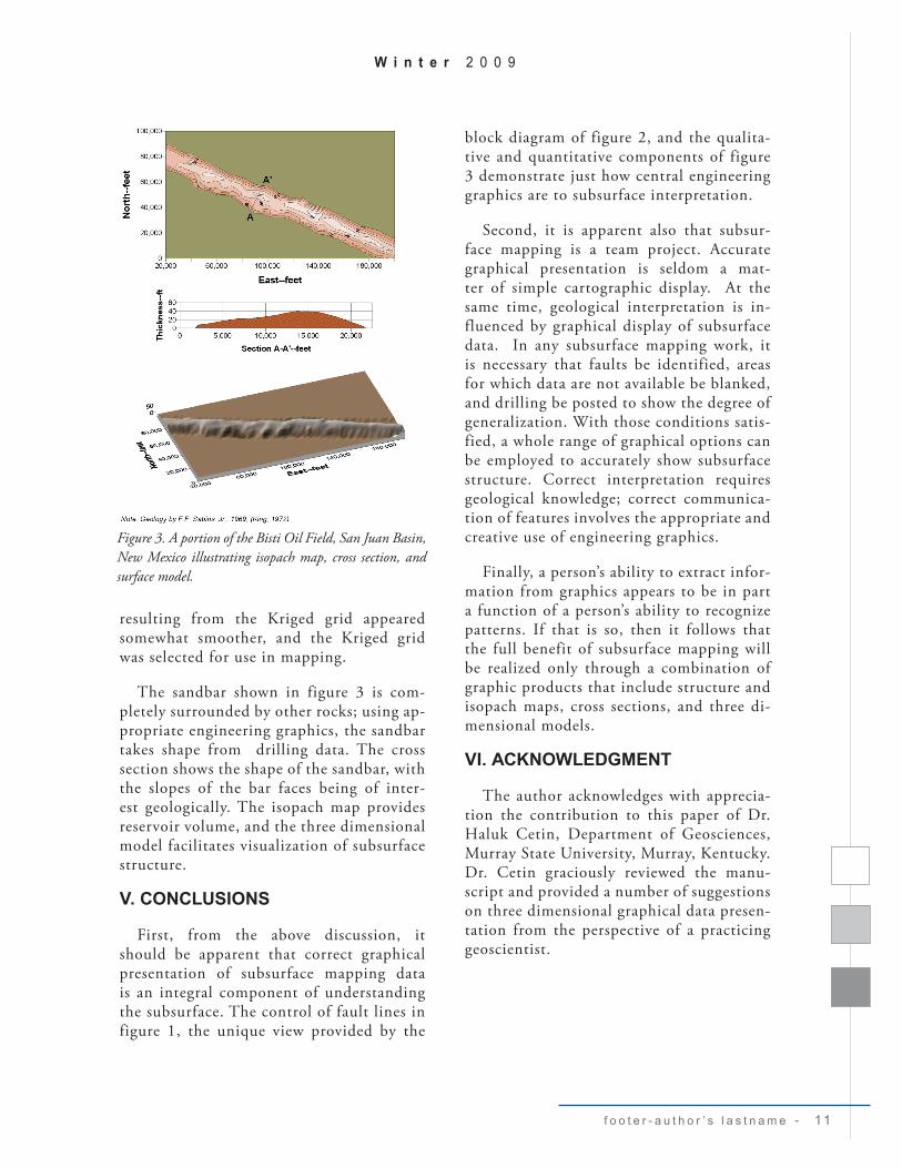
Figure 3 shows an isopach map, a cross section, and a surface model for a sand-bar in the Bisti Field, San Juan Basin, New Mexico. Geology of this field was worked out by Sabins (in King, 1972). This field was selected for this paper because data are narrowly distributed in an essentially linear band. The resulting anistrophy can make it difficult to contour the data correctly. Because of this, two different gridding al-gorithms—minimum curvature and Krig-ing—were used to grid the data. Isopachs

Figure 2. Block diagram showing composite surface models based for a portion of the Illinois Basin Coal Field, Muhlenberg County, Kentucky.

f o o t e r - a u t h o r ’ s l a s t n a m e - 11

W i n t e r 2 0 0 9

resulting from the Kriged grid appeared somewhat smoother, and the Kriged grid was selected for use in mapping.

The sandbar shown in figure 3 is com-pletely surrounded by other rocks; using ap-propriate engineering graphics, the sandbar takes shape from drilling data. The cross section shows the shape of the sandbar, with the slopes of the bar faces being of inter-est geologically. The isopach map provides reservoir volume, and the three dimensional model facilitates visualization of subsurface structure.

V. CONCLUSIONS

First, from the above discussion, it should be apparent that correct graphical presentation of subsurface mapping data is an integral component of understanding the subsurface. The control of fault lines in figure 1, the unique view provided by the

block diagram of figure 2, and the qualita-tive and quantitative components of figure 3 demonstrate just how central engineering graphics are to subsurface interpretation.

Second, it is apparent also that subsur-face mapping is a team project. Accurate graphical presentation is seldom a mat-ter of simple cartographic display. At the same time, geological interpretation is in-fluenced by graphical display of subsurface data. In any subsurface mapping work, it is necessary that faults be identified, areas for which data are not available be blanked, and drilling be posted to show the degree of generalization. With those conditions satis-fied, a whole range of graphical options can be employed to accurately show subsurface structure. Correct interpretation requires geological knowledge; correct communica-tion of features involves the appropriate and creative use of engineering graphics.

Finally, a person’s ability to extract infor-mation from graphics appears to be in part a function of a person’s ability to recognize patterns. If that is so, then it follows that the full benefit of subsurface mapping will be realized only through a combination of graphic products that include structure and isopach maps, cross sections, and three di-mensional models.

VI. ACKNOWLEDGMENT

The author acknowledges with apprecia-tion the contribution to this paper of Dr. Haluk Cetin, Department of Geosciences, Murray State University, Murray, Kentucky. Dr. Cetin graciously reviewed the manu-script and provided a number of suggestions on three dimensional graphical data presen-tation from the perspective of a practicing geoscientist.

Figure 3. A portion of the Bisti Oil Field, San Juan Basin, New Mexico illustrating isopach map, cross section, and surface model.

1 2 - E n g i n e e r i n g D e s i g n G r a p h i c s J o u r n a l

v o l u m e 7 3 n u m b e r 1

REFERENCES

Abramowitz, M. & Stegun, I. (1972). Hand-book of mathematical functions. New York, NY: Dover.

Ali, M., Chawathe, A., Ouenes, A., Cather, M., & Weiss, W. (1999) Extracting maxi-mum geological information from a lim-ited reservoir database. In R.A. Schatz-inger & J.F. Jordan (Eds.), Reservoir characterization—recent advances. Tulsa, OK: Memoir 71, American Association of Petroleum Geologists.

Barnes, J.W. & Lisle, R.J. (2004). Basic geological mapping. (4th ed.). Chicester, England: Wiley.

Brewer, C.A. (1994). Color use guidelines for mapping and visualization. In A.M. MacEachren and D.R.F. Taylor (Eds.), Visualization in Modern Cartography. Oxford, UK: Pergamon.

Briggs, I.C. (1974). Machine contouring using minimum curvature. Geophysics, 39(1), 39-48.

Cressie, N.A.C. (1990). The origins of Kriging. Mathematical Geology, 22, 239-252.

Cressie, N.A.C. (1991). Statics for spatial data. New York, NY: Wiley.

Davis, J.C. (1986). Statistics and data anal-ysis in geology. New York, NY: Wiley.

Deutsch, C.V. & Journel, A.G. (1992). GSLID—geostatistical software library and user’s guide. New York, NY: Oxford.

Franke, R. (1982). Scattered data interpola-tion: test of some methods. Mathematics of Computations, 33(157), 181-200.

Golden Software (2002). Surfer. (version

8). Golden, Co.

Golden Software (2004). Didger. (version 2). Golden, Co.

Hambrey, M.J., Smellie, J.L., Nelson, A.E., & Johnson, J.S. (2008). Late Cenozoic glacier-volcano interaction on James Ross Island and adjacent areas, Antarctic Pen-insula region. Geologic Society of Amer-ican Bulletin, 120 (5/6) 709-731.

Hicks, I.C., Westheimer, J., Tomlinson, C.W., Putman, D.M., & Selk, E.L. (Eds.). (1956). Petroleum geology of southern Oklahoma. (Vol. 1). Tulsa, OK: Ameri-can Association of Petroleum Geologists.

Hudson, M.R., Grauch, V.J.S., & Minor, S.A. (2008). Rock magnetization charac-terization of faulted sediments in the Al-buquerque Basin, Rio Grande rift, New Mexico. Geologic Society of American Bulletin, 120 (5/6) 641-658.

Isaaks, E.H. & Srivastava, R.M. (1989). An introduction to applied geostatics. New York, NY: Oxford.

Jones, T.A., Hamilton, D.E., & Johnson, C.R. (1986). Contouring geologic sur-faces with the computer. New York, NY: Van Nostrand Reinhold.

Journel, A.G. & Huijbregts, C. (1978). Mining geostatistics. New York, NY: Aca-demic Press.

Journal, A.G. (1989). Fundamental of geo-statistics in five lessons. Washington, D.C.: American Geophysical Union.

Kellie, A.C., Jordan, F.M., & Whitaker, W. (2007). Geotechnical data presentation and earth volume estimates—surveying in three dimensions. Proceedings, An-nual Meeting of the American Congress on Surveying and Mapping, St. Louis, 11 pp. http://www.acsm.net/sessions07/kel-

f o o t e r - a u t h o r ’ s l a s t n a m e - 1 3

W i n t e r 2 0 0 9

lie311.pdf

Knox, P.R. & Barton, M.D. (1999). Pre-dicting internal heterogeneity in fluvial-deltaic reservoirs In Schatzinger, R.A. & Jordan, J.F. (1999). Reservoir charac-terization—recent advances. Tulsa, OK: Memoir 71, American Association of Pe-troleum Geologists.

Leonardson, R.W., Weakly, C.G., Lander, A.M., & Zoar, P.B. (2006, December). Exploring between drill holes yields new ounces at Goldstrike. Mining Engineer-ing ,47, 37-40.

MacEachren, A.M. (1995). How maps work. New York, NY: Guilford.

Palmer, J.E. (1969). Geologic map of the Central City West Quadrangle, Muhlen-berg and Ohio Counties, Kentucky. Wash-ington, D.C.: U.S. Geological Survey.

Press, W.H., Flannery, B.P., Tuekolsky, S.A., & Vetterling, W.T. (1988). Numerical recipes in C. Cambridge, U.K.: Cam-bridge University Press.

Resor, P.G. (2008). Deformation associated with a continental normal fault system, western Grand Canyon, Arizona. Geo-logical Society of America Bulletin, 120 (3/4), 414-430.

Sabins, F.F. (1972). Comparison of Bisti and Horseshoe Canyon stratigraphic traps, San Juan Basin, New Mexico. In R.E. King (Ed.), Stratigraphic oil and gas fields. Tulsa, OK: Memoir 16, American Association of Petroleum Geologists.

Smith, W.H.F. & Wessel, P. (1990). Grid-ding with continuous curvature splines in tension. Geophysics, 55(3) 293-305.

West, T.R. (1995). Geology applied to engi-neering. Englewood Cliffs, NJ: Prentice-Hall.