Subject Name: Structure Analysis- I Subject Code- CE4005

UNIT-I Virtual work and Energy Principles: Principles of Virtual work applied to deformable bodies, strain e e g a d o ple e ta e e g , E e g theo e s, Ma ell s Re ip o al theo e , A al sis of Pi -Jointed frames for static loads.

Energy Methods in Structural Analysis Virtual Work Introduction

. F o Castiglia o s theo e it follo s that fo the stati all dete i ate st u tu e; the pa tial derivative of strain energy with respect to external force is equal to the displacement in the direction of that load. In this lesson, the principle of virtual work is discussed. As compared to other methods, virtual work methods are the most direct methods for calculating deflections in statically determinate and indeterminate structures. This principle can be applied to both linear and nonlinear structures. The principle of virtual work as applied to deformable structure is an extension of the virtual work for rigid bodies. This may be stated as: if a rigid body is in equilibrium under the action of a system of forces and if it continues to remain in equilibrium if the body is given a small (virtual) displacement, the the i tual o k do e the F−F−s ste of fo es as it ides alo g these i tual displa e e ts is zero.

Complementary Strain Energy:

Consider the stress strain diagram as shown Fig 1.1. The area enclosed by the inclined line and the vertical axis is called the complementary strain energy. For a linearly elastic material the complementary strain energy and elastic strain energy are the same.

Figure 1.1: Stress strain diagram.

Let us consider elastic nonlinear prismatic bar subjected to an axial load. The resulting stress strain plot is as shown.

Page no: 1

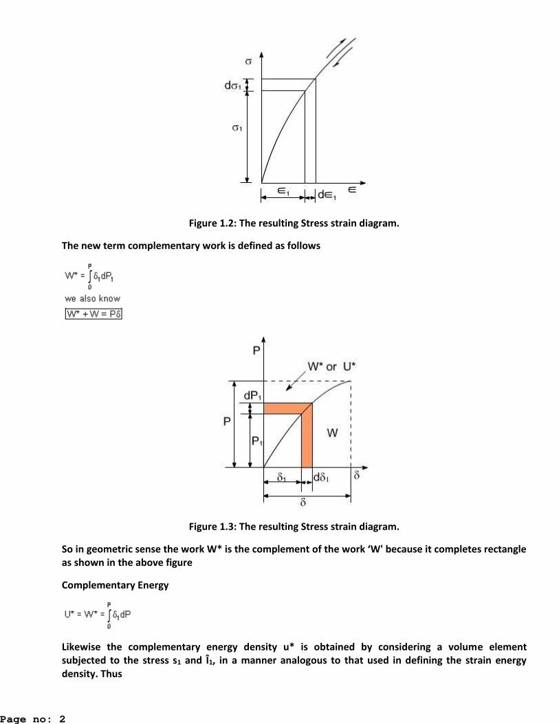
Figure 1.2: The resulting Stress strain diagram.

The new term complementary work is defined as follows

Figure 1.3: The resulting Stress strain diagram.

So in geo et i se se the o k W* is the o ple e t of the o k W' e ause it o pletes e ta gle as shown in the above figure

Complementary Energy

Likewise the complementary energy density u* is obtained by considering a volume element subjected to the stress s1 and Î1, in a manner analogous to that used in defining the strain energy density. Thus

Page no: 2

The complementary energy density is equal to the area between the stress strain curve and the stress axis. The total complementary energy of the bar may be obtained from u* by integration

Sometimes the complementary energy is also called the stress energy. Complementary Energy is expressed in terms of the load and that the strain energy is expressed in terms of the displacement.

Castigliano's Theorem: Strain energy techniques are frequently used to analyze the deflection of beam and structures. Castigliano's theorem were developed by the Italian engineer Alberto Castigliano in the year 1873, these theorems are applicable to any structure for which the force deformation relations are linear

Castigliano's Theorem:

Figure 1.4: The loaded beam.

Consider a loaded beam as shown in figure 1.4

Let the two Loads P1 and P2 produce deflections Y1 and Y2 respectively strain energy in the beam is equal to the work done by the forces.

Let the Load P1 be increased by an amount DP1.

Let DP1 and DP2 be the corresponding changes in deflection due to change in load to DP1.

Now the increase in strain energy

Suppose the increment in load is applied first followed by P1 and P2 then the resulting strain energy is

Since the resultant strain energy is independent of order loading,

Page no: 3

Combing equation 1, 2 and 3. One can obtain

or upon taking the limit as DP1 approaches zero [ Partial derivative are used because the strain energy is a function of both P1 and P2 ]

For a general case there may be number of loads, therefore, the equation (6) can be written as

The above equation is castigation's theorem:

The statement of this theorem can be put forth as follows; if the strain energy of a linearly elastic structure is expressed in terms of the system of external loads. The partial derivative of strain energy with respect to a concentrated external load is the deflection of the structure at the point of application and in the direction of that load.

In a similar fashion, Castiglia o s theorem can also be valid for applied moments and resulting rotations of the structure

Where

Mi = applied moment

qi = resulting rotation

Castigliano's First Theorem:

Page no: 4

In similar fashion as discussed in previous section suppose the displacement of the structure are changed by a small amount ddi. While all other displacements are held constant the increase in strain energy can be expressed as

Where

¶U / di ® is the rate of change of the strain energy w.r.t di.

It may be seen that, when the displacement di is increased by the small amount dd ; work done by the corresponding force only since other displacements are not changed.

The work which is equal to Piddi is equal to increase in strain energy stored in the structure

By rearranging the above expression, the Castigliano's first theorem becomes

The above relation states that the partial derivative of strain energy w.r.t. any displacement d i is equal to the corresponding force Pi provided that the strain is expressed as a function of the displacements.

Maxwell-Betti Law of Reciprocal Deflections

Maxwell-Betti Law of real work is a basic theorem in the structural analysis. Using this theorem, it will be established that the flexibility coefficients in compatibility equations, formulated to solve indeterminate structures by the flexibility method, form a symmetric matrix and this will reduce the number of deflection computations. The Maxwell-Betti law also has applications in the construction of influence lines diagrams for statically indeterminate structures. The Maxwell-Betti law, which applies to any stable elastic structure (a beam, truss, or frame, for example) on unyielding supports and at constant temperature, states:

The deflection of point A in direction 1 due to unit load at point B in direction 2 is equal in the magnitude to the deflection of point B in direction 2 produced by a unit load applied at A in direction 1.

The Figure 4.31 explains the Maxwell-Betti Law of reciprocal displacements in which, the

displacement is equal to the displacement.

Page no: 5

In order to prove the reciprocal theorem, consider the simple beams shown in Figure 4.32. Let a

vertical force at point B produces a vertical deflection at point A and at point B as shown

in Figure 4.32(a). Similarly, in Figure 4.32(b) the application of a vertical force at point A produces

a vertical deflections and at points A and B, respectively. Let us evaluate the total work done

by the two forces and when they are applied in different order to the zero to their final value.

Case 1: applied and followed by

(a) Work done when is gradually applied

s

Page no: 6

(b) Work done when is gradually applied with in place

Total work done by the two forces for case 1 is

Page no: 7

Case2: applied and followed by

(c) Work done when is gradually applied

(d) Work done when is gradually applied with in place

Total work done by the two forces for case 2 is

Since the final deflected position of the beam produced by the two cases of loads is the same

regardless of the order in which the loads are applied. The total work done by the forces is also the

same regardless of the order in which the loads are applied. Thus, equating the total work of Cases 1

and 2 give

If , the equation (4.31) depicts the statement of the Maxwell-Betti law i.e.

The Maxwell-Betti theorem also holds for rotations as well as rotation and linear displacement in beams and frames.

Example 4.21 Verify Maxwell-Betti law of reciprocal displacement for the direction 1 and 2 of the pin-jointed structure shown in Figure (a).

Page no: 8

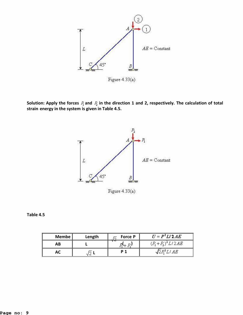
Solution: Apply the forces and in the direction 1 and 2, respectively. The calculation of total strain energy in the system is given in Table 4.5.

Table 4.5

Member

Length Force P

AB

L -( )

AC L P 1

Page no: 9

Since , hence the Maxwell-Betti law of reciprocal displacement is proved.

Example: Verify Maxwell-Betti law of reciprocal displacement for the cantilever beam shown in Figure 4.34(a).

Solution: Apply the forces and in the directions 1 and 2, respectively. The total strain energy stored is calculated below.

Consider any point X at a distance x from B.

Page no: 10

Since , the Maxwell-Betti law of reciprocal displacement is proved.

Example: Verify Maxwell-Betti law of reciprocal displacement for the rigid-jointed plane frame with reference to marked direction as shown in Figure 4.35(a). EI is same for both members.

Solution: Apply the forces and in the directions 1 and 2, respectively as shown in Figure (b).

Page no: 11

Consider AB: (x measured from A)

Consider BC: (x measured from B)

Thus

The displacement in the direction 1 due to unit load applied in 2 is

Page no: 12

The displacement in the direction 2 due to unit load applied in 1 is

Since , proves the Maxwell-Betti law of reciprocal displacements.

Page no: 13

Unit II

Indeterminate Structures-I: Static and Kinematics indeterminacy, Analysis of Fixed and

continuous beams by theorem of three moments, Effect of sinking and rotation of supports,

Moment distribution method (without sway)

Three Moment Equation

The continuous beams are very common in the structural design and it is necessary to

develop simplified force method known as three moment equation for their analysis. This

equation is a relationship that exists between the moments at three points in continuous

beam. The points are considered as three supports of the indeterminate beams. Consider

three points on the beam marked as 1, 2 and 3 as shown in Figure (a). Let the bending

moment at these points is M1, M2 and M3, and the corresponding vertical displacement of

these poi ts a e Δ1, Δ2a d Δ3, respectively. Let L1 and L2 be the distance between points 1 –

2 and 2 – 3, respectively.

The continuity of deflected shape of the beam at point 2 gives

Θ21 = θ23 Equations 5.4

Page no: 14

From the Figure 5.25(d)

Θ21 = θ1 – β21 a d Θ23 = θ3 – β23

Where

Θ1 = Δ1 – Δ2)/L1 a d Θ3 = Δ3 – Δ2)/L2

Using the bending moment diagrams shown in Figure 5.25(c) and the second moment area

theorem,

Θ21 = [1/(L1*E*I1)]*{(M1L12/6) +(M2L1

2/3) + (A1X1 ] Equations 5.7

Θ23 = [1/(L2*E*I2)]*{(M3L12/6) +(M2L1

2/3) + (A2X2 ] Equations 5.8

Where A1 and A2 are the areas of the bending moment diagram of span 1-2 and 2-3,

respectively considering the applied loading acting as simply supported beams.

Substituting from Equation (5.7) and Equation (5.8) in Equation (5.4) and Equation (5.5).

M1(L1/I1) + 2M2[(L1/I1) + (L2/I2)] + M3(L2/I2) = -6*A1*X1 / I1*L1) –

6*A2*X2 / I2*L2 + *E [ Δ2 – Δ1)/L1 + [ Δ2 – Δ3)/L2]

The above is known as three moment equation.

Sign Conventions

The M1, M2 and M3 are positive for sagging moment and negative for hogging moment.

Similarly, areas A1, A2 and A3 are positive if it is sagging moment and negative for hogging

o e t. The displa e e ts Δ , Δ a d Δ a e positi e if easu ed do a d f o the reference axis.

MOMENT DISTRIBUTION METHOD

Introduction

In the previous lesson we discussed the slope-deflection method. In slope-deflection analysis, the unknown displacements (rotations and translations) are related to the applied loading on the structure. The slope-deflection method results in a set of simultaneous equations of unknown displacements. The number of simultaneous equations will be equal to the number of unknowns to be evaluated. Thus one needs to solve these simultaneous equations to obtain displacements and beam end moments. Today, simultaneous equations could be solved very easily using a computer. Before the advent of electronic computing, this really posed a problem as the number of equations in the case of multistory building is quite large. The moment-distribution method proposed by Hardy Cross in 1932, actually solves these equations by the method of successive approximations. In this method, the results may be obtained to any desired degree of accuracy. Until recently, the moment-distribution method was very popular among

Page no: 15

engineers. It is very simple and is being used even today for preliminary analysis of small structures. It is still being taught in the classroom for the simplicity and physical insight it gives to the analyst even though stiffness method is being used more and more. Had the computers not emerged on the scene, the moment-distribution method could have turned out to be a very popular method. In this lesson, first moment-distribution method is developed for continuous beams with unyielding supports.

Basic Concepts

In moment-distribution method, counterclockwise beam end moments are taken as positive. The counterclockwise beam end moments produce clockwise moments on the joint Consider a continuous beam ABCD as shown in Fig.18.1a. In this beam, ends A and D are fixed and hence, θ A = θ D = 0 .Thus, the deformation of this beam is completely defined by rotations θ B and C respectively. The required equation to e aluate θ B and considering equilibrium of joints B and C. Hence,

∑M B = 0 ⇒ M BA + M BC = 0 (18.1a)

∑M C = 0 ⇒ M CB + M CD = 0 (18.1b)

According to slope-deflection equation, the beam end moments are written as

MBA = MFBA + EI/L θB + θA)

(4EI/L) is known as stiffness factor for the beam AB and it is denoted by k AB. M BAF is the

fixed end moment at joint B of beam AB when joint B is fixed.

Thus,

M BA = M BAF + K ABθ B

M CD = M CDF + KCDθC (18.2)

In Fig.18.1b, the counterclockwise beam-end moments M BA and

M BC

produce

A clockwise moment M B on the joint as shown in Fig.18.1b. To start with, in moment-distribution method, it is assumed that joints are locked i.e. joints are prevented from rotating. In such a case (vide Fig.18.1b),

θ B = θ C = 0 , and hence

M BA = M BAF

M BC = M BCF

M CB = M CBF

M CD = M CDF (18.3)

Page no: 16

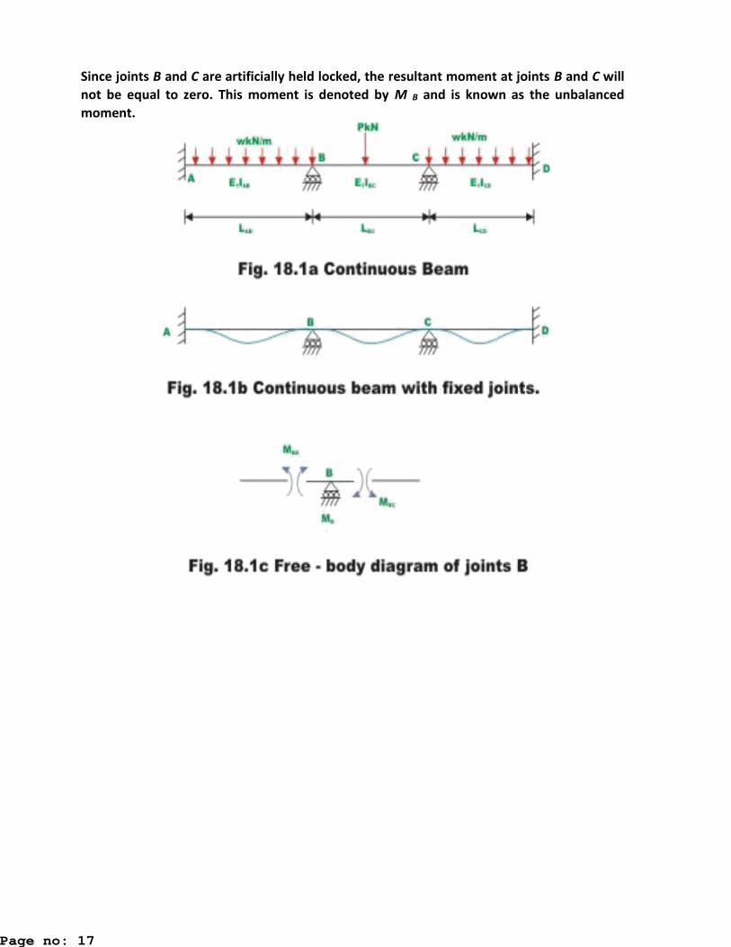
Since joints B and C are artificially held locked, the resultant moment at joints B and C will

not be equal to zero. This moment is denoted by M B and is known as the unbalanced

moment.

Page no: 17

Thus,

M B = M BAF + M BC

F

In reality joints are not locked. Joints B and C do rotate under external loads. When the

joint B is unlocked, it will rotate under the action of unbalanced moment M B. Let the joint

B rotate by an angle θ B1, under the action of M B. This will deform the structure as shown

in Fig.18.1d and introduces distributed moment M BAd

, M BCd in the span BA and BC

respectively as shown in the figure.

The unknown distributed moments are assumed to be positive and hence act in counterclockwise direction. The unbalanced moment is the algebraic sum of the fixed end moments and act on the joint in the clockwise direction. The unbalanced moment restores the equilibrium of the joint B. Thus,

∑M B = 0, M BAd + M BC

d + M B = 0 (2.4)

The dist i uted o e ts a e elated to the otatio θB1 by the slope- deflection equation.

M BAd = K BAθ B1

M BCd = K BCθ B1 (2.5)

Substituting equation (18.5) in (18.4), yields

θB1 (K BA + K BC) = −M B

θB1 = M B/ (K BA + K BC)

In general, where summation is taken over all the members meeting at that particular joint. Substituting the value of θ B1 in equation (2.5), distributed moments are calculated. Thus, the ratio ∑KBA

K is known as the distribution factor and is represented by DFBA.

Thus, M BAd = −DFBA. M B

M BCd = −DFBC. M B (2.8)

The distribution moments developed in a member meeting at B, when the joint B is unlocked and allowed to rotate under the action of unbalanced moment M B is equal to a distribution factor times the unbalanced moment with its sign reversed.

As the joint B rotates under the action of the unbalanced moment, beam end moments are

developed at ends of members meeting at that joint and are known as distributed

moments. As the joint B rotates, it bends the beam and beam end moments at the far ends

(i.e. at A and C) are developed. They are known as carry over moments. Now consider the

beam BC of continuous beam ABCD.

When the joint B is unlocked, joint C is locked .The joint B rotates by θ B1 under the action

of unbalanced moment M B (vide Fig. 18.1e). Now from slope-deflection equations

Page no: 18

The carry over moment is one half of the distributed moment and has the same sign. With

the above discussion, we are in a position to apply moment-distribution method to

statically indeterminate beam. Few problems are solved here to illustrate the procedure.

Carefully go through the first problem, wherein the moment-distribution method is

explained in detail.

Example

A continuous prismatic beam ABC (see Fig.2.2a) of constant moment of inertia is carrying a

uniformly distributed load of 2 kN/m in addition to a concentrated load of 10 kN. Draw

bending moment diagram. Assume that supports are unyielding

Solution

Assuming that supports B and C are locked, calculate fixed end moments developed in the beam due to externally applied load. Note that counterclockwise moments are taken as

positive.

MAB = 1.5 kN M.

MBA = - 1.5 kN M.

MBC = 5 kN M.

MCB = -5 kN M.

Before we start analyzing the beam by moment-distribution method, it is required to

calculate stiffness and distribution factors.

At C: ∑ K = EI

DFCB = 1.0

Note that distribution factor is dimensionless. The sum of distribution factor at a joint, except when it is fixed is always equal to one. The distribution moments are developed only when the joints rotate under the action of unbalanced moment. In the case of fixed joint, it does not rotate and hence no distribution moments are developed and consequently distribution factor is equal to zero.

In Fig.18.2b the fixed end moments and distribution factors are shown on a working

diagram. In this diagram B and C are assumed to be locked.

Now unlock the joint C. Note that joint C starts rotating under the unbalanced moment of 5 kN.m (counterclockwise) till a moment of -5 kN.m is developed (clockwise) at the joint.

Page no: 19

This in turn develops a beam end moment of +5 kN.m (M CB). This is the distributed moment and thus restores equilibrium. Now joint C is relocked and a line is drawn below +5 kN.m to indicate equilibrium. When joint C rotates, a carryover moment of +2.5 kN.m is developed at the B end of member BC. These are shown in Fig.18.2c.

When joint B is unlocked, it will rotate under an unbalanced moment equal to algebraic sum of the fixed end moments(+5.0 and -1.5 kN.m) and a carryover moment of +2.5 kN.m till distributed moments are developed to restore equilibrium. The unbalanced moment is 6 kN.m. Now the distributed moments M BC and M BA are obtained by multiplying the unbalanced moment with the corresponding distribution factors and reversing the sign. Thus, M BC = −2.574 kN.m and M BA = −3.426kN.m. These distributed moments restore the equilibrium of joint B. Lock the joint B. This is shown in Fig.18.2d along with the carry over moments.

Now, it is seen that joint B is balanced. However joint C is not balanced due to the carry

over moment -1.287 kN.m that is developed when the joint B is allowed to rotate. The

whole procedure of locking and unlocking the joints C and B successively has to be

continued till both joints B and C are balanced simultaneously. The complete procedure is

shown in Fig.18.2e.

Page no: 20

The iteration procedure is terminated when the change in beam end moments is less than

say 1%. In the above problem the convergence may be improved if we leave the hinged end C unlocked after the first cycle. This will be discussed in the next section. In such a case

the stiffness of beam BC gets modified. The above calculations can also be done

conveniently in a tabular form as shown in Table 18.1. However the above working method is preferred in this course.

Table 18.1 Moment-distribution for continuous beam ABC

Joint A B C

Member AB BA BC CB

Stiffness 1.333EI 1.333EI EI EI

Distribution 0.571 0.429 1.0

factor

FEM +1.5 -1.5 +5.0 -5.0

kN.m

Balance +2.5 +5.0

joints C -1.713 -3.426 -2.579 0

and C.O.

-4.926 +4.926

-1.287

Balance +0.644

1.287

and C.O.

Bala -0.368 -0.276 -

0.13

Page no: 21

nce 8

and C.O.

Balance C -0.184 -5.294 +5.294

0.138

C.O. +0.069 0

Balance -0.02 -0.039 -0.030

-0.015

and C.O.

Balance C

+0.015

Balanced -0.417 -5.333 +5.333 0

moments in

kN.m

Example

Draw the bending moment diagram for the continuous beam ABCD loaded as shown in

Fig.18.4a.The relative moment of inertia of each span of the beam is also shown in the

figure.

Solution

Page no: 22

Note that joint C is hinged and hence stiffness factor BC gets modified. Assuming that the

supports are locked, calculate fixed end moments. They are

M ABF = 16 kN.m

MBAF = −16 kN.m

MBCF = 7.5 kN.m

MCBF = −7.5 kN.m, and

MCDF = 15 kN.m

In the next step calculate stiffness and distribution factors

Now all the calculations are shown in Fig.18.4b

This problem has also been solved by slope-deflection method (see example 14.2).The

bending moment diagram is shown in Fig.18.4c.

Summary

An introduction to the moment-distribution method is given here. The moment-

distribution method actually solves these equations by the method of successive

approximations. Various terms such as stiffness factor, distribution factor, unbalanced moment, distributing moment and carry-over-moment are defined in this lesson.

Page no: 23

Unit III

Indeterminate Structures - II: Analysis of beams and frames by slope Deflection method, Column Analogy method.

Slope deflection Method

Introduction

As pointed out earlier, there are two distinct methods of analysis for statically indeterminate structures depending on how equations of equilibrium, load displacement and compatibility conditions are satisfied: 1) force method of analysis and (2) displacement method of analysis. In the last module, force method of analysis was discussed. In this module, the displacement method of analysis will be discussed. In the force method of analysis, primary unknowns are forces and compatibility of displacements is written in terms of pre-selected redundant reactions and flexibility coefficients using force displacement relations. Solving these equations, the unknown redundant reactions are evaluated. The remaining reactions are obtained from equations of equilibrium.

As the name itself suggests, in the displacement method of analysis, the primary unknowns are displacements. Once the structural model is defined for the problem, the unknowns are automatically chosen unlike the force method. Hence this method is more suitable for computer implementation. In the displacement method of analysis, first equilibrium equations are satisfied. The equilibrium of forces is written by expressing the unknown joint displacements in terms of load by using load displacement relations. These equilibrium equations are solved for unknown joint displacements. In the next step, the unknown reactions are computed from compatibility equations using force displacement relations. In displacement method, three methods which are closely related to each other will be discussed.

1. Slope-Deflection Method

2. Moment Distribution Method

3. Direct Stiffness Method

In this module first two methods are discussed and direct stiffness method is treated in the

next module. All displacement methods follow the above general procedure. The Slope-

deflection and moment distribution methods were extensively used for many years before

the compute era. After the revolution occurred in the field of computing only direct

stiffness method is preferred.

Degrees of freedom

In the displacement method of analysis, primary unknowns are joint displacements which

are commonly referred to as the degrees of freedom of the structure. It is necessary to

consider all the independent degrees of freedom while writing the equilibrium equations.

These degrees of freedom are specified at supports, joints and at the free ends. For

example, a propped cantilever beam (see Fig.14.01a) under the action of load P will

Page no: 24

undergo only rotation at B if axial deformation is neglected. In this case kinematic degree

of freedom of the beam is only one i.e. θB as shown in the figure.

In Figur 14.01 (b), we have nodes at A, B, C and D. Under the action of lateral loads, P1, P2 and P3 , this continuous beam deform as shown in the figure. Here axial deformations are neglected. For this beam we have five degrees of freedom θ A, θB, θB, θ D and D as indicated in the figure. In Fig.14.02a, a symmetrical plane frame is loaded symmetrically. In this case we have only two degrees of freedom θ B and θC. Now consider a frame as shown in Fig.14.02b. It has three degrees of freedom viz. θ B, θC and D as shown. Under the action of horizontal and vertical load, the frame will be displaced as shown in the figure. It is observed that nodes at B and C undergo rotation and also get displaced horizontally by an equal amount.

Figure 14.01: Derivation of slope – deflection equation.

Hence in plane structures, each node can have at the most one linear displacement and

one rotation. In this module first slope-deflection equations as applied to beams and rigid

frames will be discussed.

Slope-Deflection Equations

Consider a typical span of a continuous beam AB as shown in Fig.14.1.The beam has constant flexural rigidity EI and is subjected to uniformly distributed loading and concentrated loads as shown in the figure. The beam is kinematically indeterminate to

Page no: 25

second degree. In this lesson, the slope-deflection equations are derived for the simplest case i.e. for the case of continuous beams with unyielding supports. In the next lesson, the support settlements are included in the slope-deflection equations.

For this problem, it is required to derive relation between the joint end moments M AB and

M BA in terms of joint rotations θA and θ B and loads acting on the beam .Two subscripts

are used to denote end moments. For example, end moments MAB denote moment acting

at joint A of the member AB. Rotations of the tangent to the elastic curve are denoted by

one subscript. Thus, θA denotes the rotation of the tangent to the elastic curve at A. The

following sign conventions are used in the slope-deflection equations (1) Moments acting

at the ends of the member in counterclockwise direction are taken to be positive. (2) The

rotation of the tangent to the elastic curve is taken to be positive when the tangent to the

elastic curve has rotated in the counterclockwise direction from its original direction. The

slope-deflection equations are derived by superimposing the end moments developed due

to (1) applied loads (2) rotation θA (3)

Rotation θ B. This is shown in Fig.14.2 (a)-(c). In Fig. 14.2(b) a kinematically determinate structure is obtained. This condition is obtained by modifying the support conditions to fixed so that the unknown joint rotations become zero. The structure shown in Fig.14.2 (b) is known as kinematically determinate structure or restrained structure. For this case, the end moments are denoted by M AB

F and M BAF. The fixed end moments are evaluated by

force–method of analysis as discussed in the previous module. For example for fixed- fixed beam subjected to uniformly distributed load, the fixed-end moments are shown in Fig.14.3.

Page no: 26

The fixed end moments are required for various load cases. For ease of calculations, fixed end forces for various load cases are given at the end of this lesson. In the actual structure end A rotates by θA and end B rotates by θB. Now it is required to derive a relation relating θA and θB with the end moments M ′AB and M ′BA. Towards this end, now consider a simply supported beam acted by moment M AB′ at A as shown in Fig. 14.4. The end moment M AB′ deflects the beam as shown in the figure. The rotations θA′ a d θB′ a e al ulated f o moment-area theorem.

Θ A = M AB*L)(3EI) 3.1a

Θ B = M AB*L)(6EI) 3.1b

Now a similar relation may be derived if only M BA′ is a ti g at e d B (see Fig. 14.4).

Θ”B = M BA*L)(3EI) 3.2a

Θ”A = M BA*L)(6EI) 3.2b

Now combining these two relations, we could relate end moments acting at A and B to

rotations produced at A and B as (see Fig. 14.2c)

ΘA = M AB*L)(3EI) - M AB*L)/(6EI) 3.3a

ΘB = M BA*L)(3EI) - M BA*L)/(6EI) 3.3b

Solving for MAB and MBA i te s of θA a d θB,

M AB = EI/L θA + θB) 3.4

M BA = EI/L θB + θA) 3.5

Now writing the equilibrium equation for joint moment at A (see Fig. 14.2).

MAB = MFAB + M AB 3.6a

Similarly writing equilibrium equation for joint B

MBA = MFBA + M BA 3.6b

Su stituti g the alues of M AB a d M BA

MAB = MFAB + EI/L θA + θB) 3.7a

Page no: 27

MBA = MFBA + EI/L θB + θA) 3.7b

Sometimes one end is referred to as near end and the other end as the far end. In that case, the above equation may be stated as the internal moment at the near end of the span is equal to the fixed end moment at the near end due to external loads plus 2

LEI times

the sum of twice the slope at the near end and the slope at the far end. The above two equations (14.7a) and (14.7b) simply referred to as slope–deflection equations. The slope-deflection equation is nothing but a load displacement relationship.

3.3 Application of Slope-Deflection Equations to Statically Indeterminate Beams

The procedure is the same whether it is applied to beams or frames. It may be summarized

as follows:

1) Identify all kinematic degrees of freedom for the given problem. This can be done by drawing the deflection shape of the structure. All degrees of freedom are treated as unknowns in slope-deflection method.

2) Determine the fixed end moments at each end of the span to applied load. The table given at the end of this lesson may be used for this purpose.

3) Express all internal end moments in terms of fixed end moments and near end, and far end joint rotations by slope-deflection equations.

4) Write down one equilibrium equation for each unknown joint rotation. For example, at a support in a continuous beam, the sum of all moments corresponding to an unknown joint rotation at that support must be zero.

5) Write down as many equilibrium equations as there are unknown joint rotations. 6) Solve the above set of equilibrium equations for joint rotations. 7) Now substituting these joint rotations in the slope-deflection equations evaluate

the end moments. 8) Determine all rotations.

Example

A continuous beam ABC is carrying uniformly distributed load of 2 kN/m in addition to a

concentrated load of 20 kN as shown in Fig.14.5a. Draw bending moment and shear force

diagrams. Assume EI to be constant.

Page no: 28

(a) Degrees of freedom

It is observed that the continuous beam is kinematically indeterminate to first degree as

only one joint rotation θ B is unknown. The deflected shape /elastic curve of the beam is

drawn in Fig.14.5b in order to identify degrees of freedom.

By fixing the support or restraining the support B against rotation, the fixed-fixed beams

area obtained as shown in Fig. C

(b). Fixed end moments M ABF , M BA

F , M BCF and M CB

F are calculated referring to the

Fig. 14 and following the sign conventions that counterclockwise moments are positive.

MFAB = (2*6*6)/12 + (20*3*3*3)(6*6) = 21 kN M.

MFBA = - 21 kN M.

MFBC = (4*4)/12 = 5.33 kN M.

MFBA = - 5.33 kN M.

(c) Slope-deflection equations

Since ends A and C are fixed, the rotation at the fixed supports is zero, θ A = θC = 0. Only

one non-zero rotation is to be evaluated for this problem. Now, write slope-deflection

equations for span AB and BC.

MAB = MFAB + EI/L ΘA + θB = + EI/ θB

MBA = MFBA + EI/L ΘB + θA) = - + EI/ θB

MBC = . + EIθB

Page no: 29

MCB = - . + . EIθB

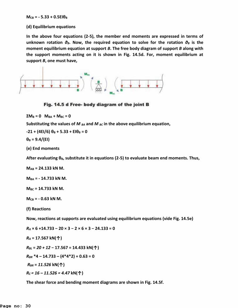
(d) Equilibrium equations

In the above four equations (2-5), the member end moments are expressed in terms of

unknown rotation θB. Now, the required equation to solve for the rotation θB is the

moment equilibrium equation at support B. The free body diagram of support B along with

the support moments acting on it is shown in Fig. 14.5d. For, moment equilibrium at

support B, one must have,

ΣMB = 0 MBA + MBC = 0

Substituting the values of M BA and M BC in the above equilibrium equation,

- + EI/ θB + . + EIθB = 0

θB = 9.4/(EI)

(e) End moments

After evaluating θB, substitute it in equations (2-5) to evaluate beam end moments. Thus,

MAB = 24.133 kN M.

MBA = - 14.733 kN M.

MBC = 14.733 kN M.

MCB = - 0.63 kN M.

(f) Reactions

Now, reactions at supports are evaluated using equilibrium equations (vide Fig. 14.5e)

RA × 6 +14.733 − 20 × 3 − 2 × 6 × 3 − 24.133 = 0

RA = 17.567 kN(↑)

RBL = 20 + 12 − 17.567 = 14.433 kN(↑)

RBR *4 – 14.733 – (4*4*2) + 0.63 = 0

RBR = 11.526 kN(↑)

RC = 16 – 11.526 = 4.47 kN(↑)

The shear force and bending moment diagrams are shown in Fig. 14.5f.

Page no: 30

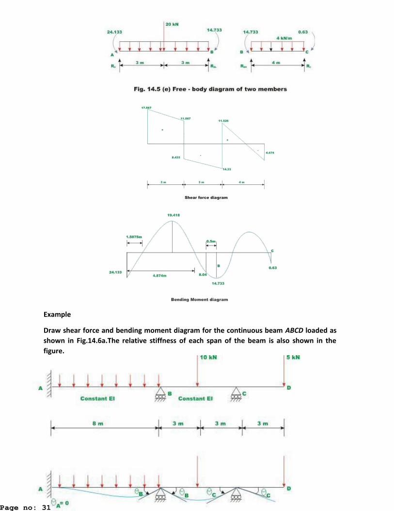
Example

Draw shear force and bending moment diagram for the continuous beam ABCD loaded as

shown in Fig.14.6a.The relative stiffness of each span of the beam is also shown in the

figure.

Page no: 31

For the cantilever beam portion CD, no slope-deflection equation need to be written as

there is no internal moment at end D. First, fixing the supports at B and C, calculate the

fixed end moments for span AB and BC. Thus,

MFAB = (3*8*8)/12 = 16 kN M.

MFBA = - 16 kN M.

MFBC = (10*3*3)(6*6) = 7.5 kN M.

MFBA = - 7.5 kN M.

In the next step write slope-deflection equation. There are two equations for each span of

the continuous beam.

MAB = + EI/L θB = + . EI θB

MAA = - + . EI θB

MBC = . + EI/L θB + θC) = . + . EI θB + . EI θC

MCB = - 7.5 + . EI θC + . EI θB

Equilibrium equations

The free body diagram of members AB, BC and joints B and C are shown in Fig.14.6b.One

could write one equilibrium equation for each joint B and C.

Support B,

ΣMB = 0 MBA + MBC = 0

ΣMC = 0 MBC + MCD = 0

We know that MCD = 15 kN.M

MCB = 15 kN.M. Substituting the values of MCB and MCD in the above equation we get

θB = . a d θC = 9.704

Substituting θB θC in the slope-deflection equations, we get

Page no: 32

MAb = 18.04 kN M.

MBA = 11.918 kN M.

MBC = - 11.918 kN M.

MCB = - 15.0 kN M.

Reactions are obtained from equilibrium equations (ref. Fig. 14.6c)

RA ×8 −18.041− 3×8 × 4 +11.918 = 0

RA =12.765 kN

RBR = 5 − 0.514kN = 4.486 kN

RBL =11.235 kN

RC = 5 + 0.514kN = 5.514 kN

The shear force and bending moment diagrams are shown in Fig. 14.6d.

Page no: 33

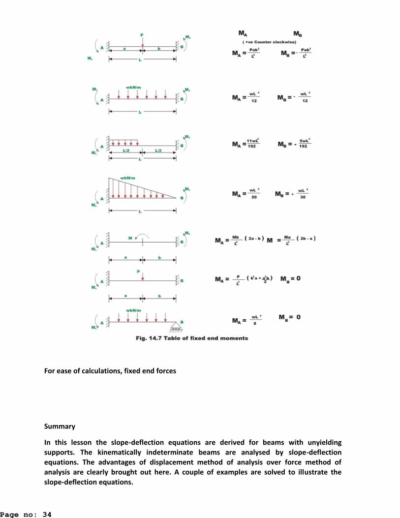
For ease of calculations, fixed end forces

Summary

In this lesson the slope-deflection equations are derived for beams with unyielding

supports. The kinematically indeterminate beams are analysed by slope-deflection

equations. The advantages of displacement method of analysis over force method of

analysis are clearly brought out here. A couple of examples are solved to illustrate the

slope-deflection equations.

Page no: 34

Column Analogy Method

Introduction

The column analogy method was also proposed by Prof. Hardy Cross and is a powerful technique to analyze the beams with fixed supports, fixed ended gable frames, closed frames & fixed arches etc., These members may be of uniform or variable moment of inertia throughout their lengths but the method is ideally suited to the calculation of the stiffness factor and the carryover factor for the members having variable moment of inertia. The method is strictly applicable to a maximum of 3rd degree of indeterminacy. This method is essentially an indirect application of the consistent deformation method.

The method is based on a mathematical similarity (i.e. analogy) between the stresses developed on a column section subjected to eccentric load and the moments imposed on a member due to fixity of its supports. In the analysis of actual engineering structures of modern times, so many analogies are used like slab analogy, and shell analogy etc. In all these methods, calculations are not made directly on the actual structure but, in fact it is always assumed that the actual structure has been replaced by its mathematical model and the calculations are made on the model. The final results are related to the actual structure through same logical engineering interpretation.

In the method of column analogy, the actual structure is considered under the action of applied loads and the redundant acting simultaneously on a BDS. The load on the top of the analogous column is usually the B.M.D. due to applied loads on simple spans and therefore the reaction to this applied load is the B.M.D. due to redundant on simple spans considers the following fixed ended loaded beam.

The esulta t of B.M.D s due to applied loads does not fall on the midpoint of analogous column section which is eccentrically loaded.

Ms diagram = BDS moment diagram due to applied loads.

Mi diagram = Indeterminate moment diagram due to redundant.

If we plot (+ve) B.M.D. above the zero li e a d − e B.M.D elo the ze o li e oth o compression sides due to two sets of loads) then we can say that these diagrams have been plotted on the compression side. (The conditions from which MA & MB can be determined, when the method of consistent deformation is used, are as follows). From the Geometry requirements, we know that

(1) The change of slope between points A & B = 0; or sum of area of moment diagrams between A & B = 0 (note that EI = Constant), or area of moment diagrams of figure b = area of moment diagram of figure c.

(2) The deviation of point B from tangent at A = 0; or sum of moment of moment diagrams between A & B about B = 0, or Moment of moment diagram of figure(b) about B = moment of moment diagram of figure (c) about B. Above two requirements can be stated as follows.

(1) Total load on the top is equal to the total pressure at the bottom and;

Page no: 35

(2) Moment of load about B is equal to the moment of pressure about B), indicates that the analogous column is on equilibrium under the action of applied loads and the redundant.

. . SIGN CONVENTIONS:− It is e essa to esta lish a sig o e tio ega di g the atu e of the applied load Ms −diag a a d the p essu es a ti g at the ase of the

a alogous olu Mi−diag a .

1. Load (P) on top of the analogous column is downward if Ms/EI diagram is (+ve) which means that it causes compression on the outside or (sagging) in BDS vice-versa. If EI is constant, it can be taken equal to units.

2. Upward pressure on bottom of the analogous column (Mi −diag a is o side ed as (+ve).

3. Moment (M) at any point of the given indeterminate structure (maximum to 3rd degree) is given by the formula.

M = Ms −Mi, which is (+ve) if it causes compression on the outside of members

In the last lesson, slope-deflection equations were derived without considering the rotation of the beam axis. In this lesson, slope-deflection equations are derived considering the rotation of beam axis. In statically indeterminate structures, the beam axis rotates due to support yielding and this would in turn induce reactions and stresses in the structure. Hence, in this case the beam end moments are related to rotations, applied loads and beam axes rotation. After deriving the slope-deflection equation in section 15.2, few problems are solved to illustrate the procedure.

Page no: 36

Now superposing the fixed end moments due to external load and end moments due to

displacements, the end moments in the actual structure is obtained .Thus (see Fig.15.1)

In the above equations, it is important to adopt consistent sign convention. In the above

derivation is taken to be negative for downward displacements. In the continuous beam

ABC, two rotations θ B and θC need to be evaluated.

Hence, beam is kinematically indeterminate to second degree. As there is no external load

on the beam, the fixed end moments in the restrained beam are zero (see Fig.15.2b).

Page no: 37

For each span, two slope-deflection equations need to be written. In span AB, B is below A. Hence, the chord AB rotates in clockwise direction. Thus, ψ AB is taken as negative. In span BC, the support C is above support B, Hence the chord joining B′C rotates in anticlockwise direction.

ψ BC = ψ CB = 1×10−3

Writing slope-deflection equations for span BC,

M BC = 0.8EIθ B + 0.4EIθC −1.2 ×10−3 EI

M CB = 0.8EIθC + 0.4EIθ B −1.2 ×10−3 EI

Now, consider the joint equilibrium of support B (see Fig.15.2c)

M BA + M BC = 0

Substituting the values of M BA and M BC in equation (6),

0.8EIθ B + 1.2 ×10−3 EI + 0.8EIθ B + 0.4EIθC −1.2 ×10−3 EI = 0

Simplifying, 1.6θ B + 0.4θC = 1.2 ×10−3

Also, the support C is simply supported and hence, M CB = 0

M CB = 0 = 0.8θC + 0.4θ B −1.2 ×10−3 EI

0.8θC + 0.4θ B = 1.2 ×10−3

We have two unknowns θ B and θC and there are two equations in θ B and θC. Solving equations (7) and (8)

Page no: 38

θ

= −0.4286 ×10−3 radians

θ= 1.7143 ×10−3 radians (9)

Substituting the values of θ B, θC and EI in slope-deflection equations,

M AB = 82.285 kN.m M BA = 68.570 kN.m

M BC = −68.573 kN.m M CB = 0 kN.m

Reactions are obtained from equations of static equilibrium (vide Fig.15.2d)

In beam AB,

∑M B = 0, RA = 30.171 kN(↑)

RBL = −30.171 kN(↓)

RBR = −13.714 kN(↓)

RC = 13.714 kN(↑)

The shear force and bending moment diagram is shown in Fig.15.2e and elastic curve is

shown in Fig.15.2f.

Page no: 39

Example

A continuous beam ABCD is carrying a uniformly distributed load of 5 kN/m as shown in

Fig.15.3a. Compute reactions and draw shear force and bending moment diagram due to

following support settlements.

Support B 0.005m vertically downwards

Support C 0.01 m vertically downwards

Assume E =200 GPa, I = 1.35 ×10−3 m4

In the above continuous beam, four rotations θ A, θ B, θC a d θD are to be evaluated. One equilibrium equation can be written at each support. Hence, solving the four equilibrium equations, the rotations are evaluated and hence the moments from slope-deflection equations. Now consider the kinematically restrained beam as shown in Fig.15.3b.

Referring to standard tables the fixed end moments may be evaluated .Otherwise one

could obtain fixed end moments from force method of analysis. The fixed end moments in

the present case are (vide fig.15.3b)

Page no: 40

M ABF = 41.667 kN.m

M BAF = −41.667 kN.m (clockwise)

M BCF = 41.667 kN.m (counterclockwise)

M CBF = −41.667 kN.m (clockwise)

M CDF = 41.667 kN.m (counter clockwise)

M DCF = −41.667 kN.m (clockwise)

In the next step, write slope-deflection equations for each span. For the span AB, B is

below A and hence the chord joining AB′ otates i the lo k ise di e tio see Fig. .

Page no: 41

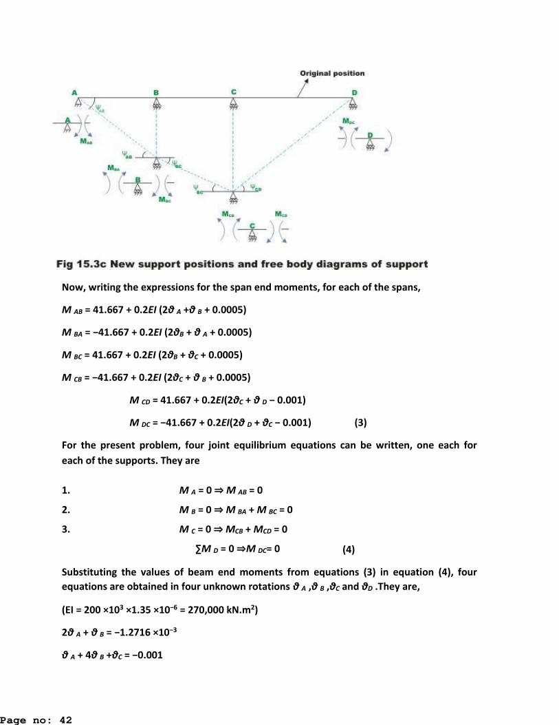
Now, writing the expressions for the span end moments, for each of the spans,

M AB = 41.667 + 0.2EI (2θ A +θ B + 0.0005)

M BA = −41.667 + 0.2EI (2θB + θ A + 0.0005)

M BC = 41.667 + 0.2EI (2θB + θC + 0.0005)

M CB = −41.667 + 0.2EI (2θC + θ B + 0.0005)

M CD = 41.667 + 0.2EI(2θC + θ D − 0.001)

M DC = −41.667 + 0.2EI(2θ D + θC − 0.001) (3)

For the present problem, four joint equilibrium equations can be written, one each for

each of the supports. They are

1. M A = 0 ⇒ M AB = 0

2. M B = 0 ⇒ M BA + M BC = 0

3. M C = 0 ⇒ MCB + MCD = 0

∑M D = 0 ⇒M DC= 0 (4)

Substituting the values of beam end moments from equations (3) in equation (4), four

equations are obtained in four unknown rotations θ A ,θ B ,θC and θD .They are,

(EI = 200 ×103 ×1.35 ×10−6 = 270,000 kN.m2)

2θ A + θ B = −1.2716 ×10−3

θ A + 4θ B +θC = −0.001

Page no: 42

θ B + 4θC + θ D = 0.0005

θC + 2θ D = 1.7716 ×10−3

Solving the above sets of simultaneous equations, values of θA, θB, θC and θD are

evaluated.

Substituting the values in slope-deflection equations the beam end moments are

evaluated.

M AB = 41.667 + 0.2 × 270,000{2(−5.9629 ×10−4) + (−7.9013 ×10−5) + 0.0005)} = 0

M BA = −41.667 + 0.2 × 270,000{2(−7.9013 ×10−5) − 5.9629 ×10−4 + 0.0005} = −55.40 kN.m

M BC = 41.667 + 0.2 × 270,000{2(−7.9013 ×10−5) + (−8.7653 ×10−5) + 0.0005} = 55.40 kN.m

M CB = −41.667 + 0.2 × 270,000{2(−8.765 ×10−5) − 7.9013 ×10−5 + 0.0005} = −28.40 kN.m

M CD = 41.667 + 0.2 × 270,000{2 × (−8.765 ×10−5) + 9.2963 ×10−4 − 0.001} = 28.40 kN.m

M DC = −41.667 + 0.2 × 270,000{2 × 9.2963 ×10−4 − 8.7653 ×10−5 − 0.001} = 0 kN.m (7)

Reactions are obtained from equilibrium equations. Now consider the free body diagram

of the beam with end moments and external loads as shown in Fig.15.3d.

RA = 19.46 kN(↑)

RBL = 30.54 kN(↑)

RBR = 27.7 kN(↑)

RCL = 22.3 kN(↑)

RCR = 27.84 kN(↑)

RD = 22.16 kN(↑)

The shear force and bending moment diagrams are shown in Fig.15.5e.

Page no: 43

Summary

In this lesson, slope-deflection equations are derived for the case of beam with yielding

supports. Moments developed at the ends are related to rotations and support settlements. The equilibrium equations are written at each support. The continuous beam

is solved using slope-deflection equations. The deflected shape of the beam is sketched. The bending moment and shear force diagrams are drawn for the examples solved in this

lesson.

Page no: 44

Unit IV

Arches and Suspension Cables: Th ee hi ged a hes of diffe e t shapes, Edd s Theo e , Suspension cable, stiffening girders, Two Hinged and Fixed Arches - Rib shortening and temperature effects

Three Hinged Arch

Introduction

In case of beams supporting uniformly distributed load, the maximum bending moment increases with the square of the span and hence they become uneconomical for long span structures. In such situations arches could be advantageously employed, as they would develop horizontal reactions, which in turn reduce the design bending moment.

For example, in the case of a simply supported beam shown in Fig. 32.1, the bending moment below the load is 3PL/16. Now consider a two hinged symmetrical arch of the same span and subjected to similar loading as that of simply supported beam. The vertical reaction could be calculated by equations of statics. The horizontal reaction is determined by the method of least work. Now the bending moment below the load is (3PL/16) Hy. It is clear that the bending moment below the load is reduced in the case of an arch as compared to a simply supported beam. It is observed in the last lesson that, the cable takes the shape of the loading and this shape is termed as funicular shape. If an arch were constructed in an inverted funicular shape then it would be subjected to only compression for those loadings for which its shape is inverted funicular.

Page no: 45

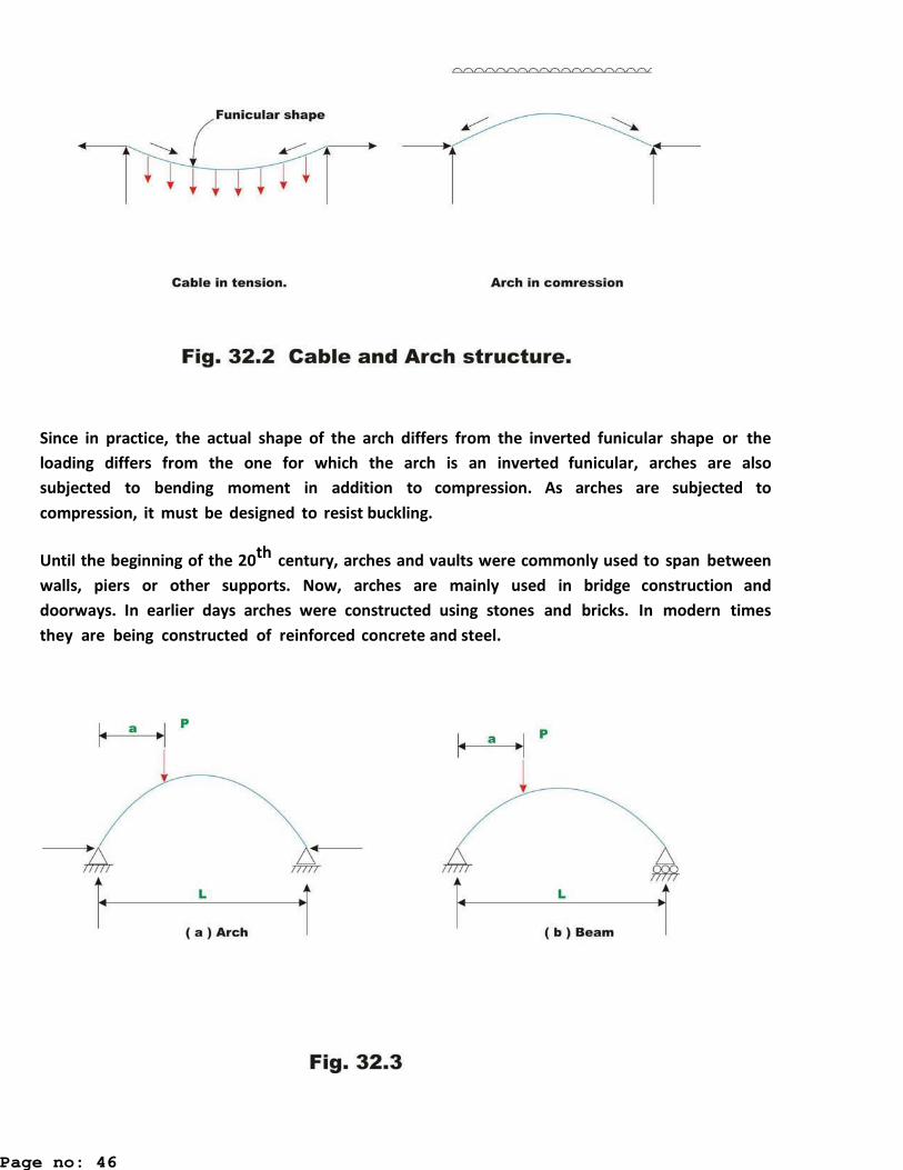
Since in practice, the actual shape of the arch differs from the inverted funicular shape or the

loading differs from the one for which the arch is an inverted funicular, arches are also

subjected to bending moment in addition to compression. As arches are subjected to

compression, it must be designed to resist buckling.

Until the beginning of the 20th century, arches and vaults were commonly used to span between

walls, piers or other supports. Now, arches are mainly used in bridge construction and

doorways. In earlier days arches were constructed using stones and bricks. In modern times

they are being constructed of reinforced concrete and steel.

Page no: 46

A structure is classified as an arch not based on its shape but the way it supports the lateral load. Arches support load primarily in compression. For example in Fig 32.3b, no horizontal reaction is developed. Consequently bending moment is not reduced. It is important to appreciate the point that the definition of an arch is a structural one, not geometrical.

Type of arches

There are mainly three types of arches that are commonly used in practice: three hinged arch, two-hinged arch and fixed-fixed arch. Three-hinged arch is statically determinate structure and its reactions / internal forces are evaluated by static equations of equilibrium. Two-hinged arch and fixed-fixed arch are statically indeterminate structures. The indeterminate reactions are determined by the method of least work or by the flexibility matrix method. In this lesson three- hinged arch is discussed.

Analysis of three-hinged arch

In the case of three-hinged arch, we have three hinges: two at the support and one at the crown thus making it statically determinate structure. Consider a three hinged arch subjected

Page no: 47

to a concentrated force P as shown in Fig 32.5.

There are four reaction components in the three-hinged arch. One more equation is required in

addition to three equations of static equilibrium for evaluating the four reaction components.

Taking moment about the hinge of all the forces acting on either side of the hinge can set up the

required equation.

Ha = Hb = PL/8h

Va + Vb = Total downwards loads

Example 32.1 A three-hinged parabolic arch of uniform cross section has a span of 60 m and a rise of 10 m. It is

subjected to uniformly distributed load of intensity 10 kN/m as shown in Fig. 32.6 Show that the

bending moment is zero at any cross section of the arch.

Reactions: Taking moment of all the forces about hinge A, yields

Va = Vb = 10*60/2 = 300 kN.

Taking moment about left hinge c, we get

Va*30 – 10*30*15 – Ha*10 = 0

Ha = Hb = 450 kN.

Page no: 48

BM at any section XX is given as

BMxx = Va*x – Ha*y – 10*x*(x/2)

The equation of the three-hinged parabolic arch is y = 4hx(L-x)/L2 substituting

BMxx = 300*x – 450(4*10*x*(60-x)) -5x2 = 300x – (450(2400x – 40x2))/(60*60) – 5x2

= 300x – 300x + 5x2 – 5x2 = 0

In other words a three hinged parabolic arch subjected to uniformly distributed load is not

subjected to bending moment at any cross section. It supports the load in pure

compression.

Example 32.2

A three-hinged semicircular arch of uniform cross section is loaded as shown in Fig 32.7.

Calculate the location and magnitude of maximum bending moment in the arch.

Solution:

Page no: 49

Reactions: Taking moment of all the forces about hinge B leads to,

Va = 29.33kN Vb = 10.67 kN.

Bending moment

Now making use of the condition that the moment at hinge of all the forces left of hinge is

zero gives, CC

Ha = Hb = 10.66 kN.

The maximum positive bending moment occurs below D and it can be calculated by taking

moment of all forces left of about D,

Y at D = 4*15*8(30-8)/302 = 13.267 m.

BM at D = Va*8 – Ha*y = 93.213 kN M.

Example 32.3

A three-hinged parabolic arch is loaded as shown in Fig 32.8a. Calculate the location and

magnitude of maximum bending moment in the arch. Draw bending moment diagram.

Solution:

Page no: 50

Reactions: Taking A as the origin, the equation of the three-hinged parabolic arch is given by,

Va = 80.0 kN Vb = 160.0 kN.

Ha = Hb = 150.0 kN.

Location of maximum bending moment Consider a section x from end B. Moment at section x in part CB of the arch is given by (please

note that B has been taken as the origin for this calculation),

BM = 160x – 150y – 10x2/2

According to calculus, the necessary condition for extreme (maximum or minimum) is that

d(BM)/dx = 0 solving we get x = 10.0 m.

BM max = 200 kN m.

Shear force at D just left of 40 kN load

Page no: 51

The slope of the a h at D is e aluated , ta θ = d /d = / – (16/400)x

Put x = . a d sol i g θ = . °

Shear force at left of D is = Ha Si θ – Va Cos θ = - 18.57 kN.

Example 32.4

A three-hinged parabolic arch of constant cross section is subjected to a uniformly distributed

load over a part of its span and a concentrated load of 50 kN, as shown in Fig. 32.9. The

dimensions of the arch are shown in the figure. Evaluate the horizontal thrust and the maximum

bending moment in the arch.

Solution:

Page no: 52

Reactions: Taking A as the origin, the equation of the parabolic arch may be written as,

Y = 4hx(L-x)/L2 = 4*3*x(20-x)/202 = -0.03x2 + 0.6x

Taking moment of all the loads about B leads to,

Va*25 + Ha*3.75 - 50*20 – 10*15*7.5 = 0

Va = (2125 – 3.75Ha)/25

Taking moment of all the forces right of hinge C about the hinge C and setting leads to,

Vb = (1125 + 6.75 Hb)/15

Ha = Hb

Va + Vb = 50 + 10*15 = 200 kN.

Substituting and solving Ha = Hb = 133.33 kN.

Va = 65.0 kN, Vb = 135.0 kN.

Page no: 53

Bending moment

From inspection, the maximum negative bending moment occurs in the region AD and the

maximum positive bending moment occurs in the region CB.

Span AD

Bending moment at any cross section in the span AD is

BM = Va*x – Ha*y = 65*x – 133.33 (-0.03x2 + 0.6x), x lies between 0 to 5

For, the maximum negative bending moment in this region, dBM/dx = 0

Solving x = 1.8748 m.

BM = - 14.06 kN M.

For the maximum positive bending moment in this region occurs at D,

BM = Vb*5 – Hb*y = 135*5 – 133.33 *(-0.03 * 5*5 + 0.6*5) = 25.0 kN M.

Span CB Bending moment at any cross section, in this span is calculated by,

BM = Va*x – Ha*(-0.03x2 + 0.6x) – 50(x – 5) – 10(x – 10) (x – 5)/2

For locating the position of maximum bending moment, dBM/dx = 0

Solving x = 17.5 m.

BM = 56.25 kN M.

Hence, the maximum positive bending moment occurs in span CB.

Summary

In this lesson, the arch definition is given. The advantages of arch construction are given in the

introduction. Arches are classified as three-hinged, two-hinged and hinge less arches. The

analysis of three-hinged arch is considered here. Numerical examples are solved in detail to show

the general procedure of three-hinged arch analysis.

Two-Hinged Arch

Introduction

Mainly three types of arches are used in practice: three-hinged, two-hinged and hinge less

arches. In the early part of the nineteenth century, three-hinged arches were commonly used for

the long span structures as the analysis of such arches could be done with confidence. However,

with the development in structural analysis, for long span structures starting from late

Page no: 54

nineteenth century engineers adopted two-hinged and hinge less arches. Two-hinged arch is the

statically indeterminate structure to degree one. Usually, the horizontal reaction is treated as the

redundant and is evaluated by the method of least work. In this lesson, the analysis of two-

hinged arches is discussed and few problems are solved to illustrate the procedure for calculating

the internal forces.

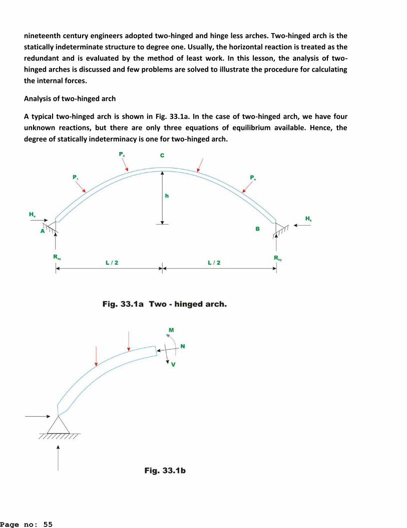
Analysis of two-hinged arch

A typical two-hinged arch is shown in Fig. 33.1a. In the case of two-hinged arch, we have four

unknown reactions, but there are only three equations of equilibrium available. Hence, the

degree of statically indeterminacy is one for two-hinged arch.

Page no: 55

The fourth equation is written considering deformation of the arch. The unknown redundant

reaction Hb is calculated by noting that the horizontal displacement of hinge bHB is zero. In

general the horizontal reaction in the two hinged arch is evaluated by straightforward

application of the theorem of least work (see module 1, lesson 4), which states that the partial

derivative of the strain energy of a statically indeterminate structure with respect to statically

indeterminate action should vanish. Hence to obtain, horizontal reaction, one must develop an

expression for strain energy. Typically, any section of the arch (vide Fig 33.1b) is subjected to

shear force V, bending moment M and the axial compression. The strain energy Ub due to

bending is calculated from the following expression.

U = ∫0s(M2/2EI) ds

The above expression is similar to the one used in the case of straight beams. However, in this

case, the integration needs to be evaluated along the curved arch length. In the above equation,

is the length of the centerline of the arch, sI is the moment of inertia of the arch cross section, E

is the You g s odulus of the a h ate ial. The st ai e e g due to shea is s all as o pa ed to the strain energy due to bending and is usually neglected in the analysis. In the case of flat

arches, the strain energy due to axial compression can be appreciable and is given by,

Ua = ∫0s(N2/2AE) ds

The total strain energy of the arch is given by,

U = ∫0s(M2/ EI ds + ∫0

s(N2/2AE) ds

No , a o di g to the p i iple of least o k ∂U/∂H = 0, where H is chosen as the redundant reaction. ∂U/∂H =∫0

s(M/EI) ∂M/∂H) ds + ∫0s(N/AE) ∂N/∂H) ds

Solving above equation, the horizontal reaction H is evaluated.

Symmetrical two hinged arch Consider a symmetrical two-hinged arch as shown in Fig 33.2a. Let at crown be the origin of co-ordinate axes. Now, replace hinge at B with a roller support. Then we get a simply supported curved beam as shown in Fig 33.2b. Since the curved beam is free to move horizontally, it will do so as shown by dotted lines in Fig 33.2b. Let M0 and No be the bending moment and axial force at any cross section of the simply supported curved beam. Since, in the original arch structure, there is no horizontal displacement, now apply a horizontal force H as shown in Fig. 33.2c. The horizontal force H should be of such magnitude, that the displacement at B must vanish.

Page no: 56

Page no: 57

From Fig. 33.2b and Fig 33.2c, the bending moment at any cross section of the arch (say),

may be written as

M = Mo – H(h – y)

The axial compressive force at any cross section (say) may be written as

N = No + H Cos θ

Whe e θ is the a gle ade the ta ge t at ith ho izo tal ide Fig . d . D Substituting the value of M and in the equation (33.4),

∂U/∂H = 0 = -∫0s(Mo – H(h – y)(h – /EI ds + ∫0

s No + H Cos θ Cos θ /AE ds

Solving for H, yields,

H = [∫0s Mo/EI ds] /[ ∫0

s 2/AE) ds]

For an arch with uniform cross section EI is constant and hence,

H = [∫0s Mo ds] /[ ∫0

s 2) ds]

In the above equation, Mo is the bending moment at any cross section of the arch when one of

the hi ges is epla ed a olle suppo t. Y is the height of the a h as sho i the figu e. If the

Page no: 58

moment of inertia of the arch rib is not constant, then equation (33.10) must be used to calculate

the horizontal reaction H.

Temperature effect Consider an unloaded two-hinged arch of span L. When the arch undergoes a uniform

temperature change of T °C, then its span would increase by TLα if it e e allo ed to expand

f eel ide Fig . a . α is the o-efficient of thermal expansion of the arch material. Since the

arch is restrained from the horizontal movement, a horizontal force is induced at the support as

the temperature is increased.

Now applying the Castiglia o s fi st theo e ,

∂U/∂H = TLα

Solving for H,

H = [TLα ] /[ ∫0s 2/EI) ds]

Page no: 59

Example 33.1 A semicircular two hinged arch of constant cross section is subjected to a concentrated load as

shown in Fig 33.4a. Calculate reactions of the arch and draw bending moment diagram.

Solution: Taking moment of all forces about hinge B leads to,

Va = 29.33 kN.

Vb = 10.67 kN.

Page no: 60

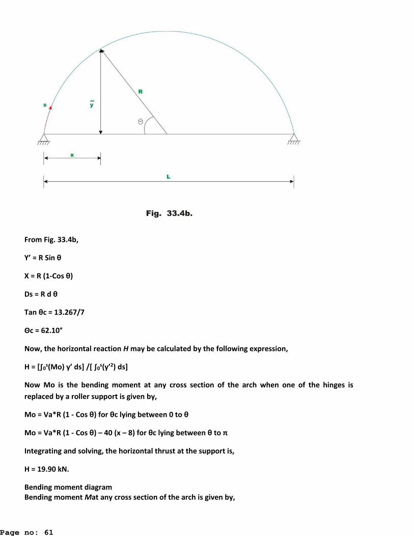
From Fig. 33.4b,

Y = R Si θ

X = R (1-Cos θ

Ds = R d θ

Ta θ = . /

Θ = . °

Now, the horizontal reaction H may be calculated by the following expression,

H = [∫0s Mo ds] /[ ∫0

s 2) ds]

Now Mo is the bending moment at any cross section of the arch when one of the hinges is

replaced by a roller support is given by,

Mo = Va*R (1 - Cos θ) for θ l i g et ee to θ

Mo = Va*R (1 - Cos θ – 40 (x – 8) for θ l i g et ee θ to π

Integrating and solving, the horizontal thrust at the support is,

H = 19.90 kN.

Bending moment diagram Bending moment Mat any cross section of the arch is given by,

Page no: 61

M = Mo – H the bending moment diagram is shown in Fig. 33.4c.

Summary

Two-hinged arch is the statically indeterminate structure to degree one. Usually, the horizontal

reaction is treated as the redundant and is evaluated by the method of least work. Towards this

end, the strain energy stored in the two-hinged arch during deformation is given. The reactions

developed due to thermal loadings are discussed. Finally, a few numerical examples are solved to

illustrate the procedure.

Cables

Introduction

Cables and arches are closely related to each other and hence they are grouped in this course in

the same module. For long span structures (for e.g. in case bridges) engineers commonly use

cable or arch construction due to their efficiency. In the first lesson of this module, cables

subjected to uniform and concentrated loads are discussed. In the second lesson, arches in

general and three hinged arches in particular along with illustrative examples are explained. In

the last two lessons of this module, two hinged arch and hinge less arches are considered.

Page no: 62

Structure may be classified into rigid and deformable structures depending on change in

geometry of the structure while supporting the load. Rigid structures support externally applied

loads without appreciable change in their shape (geometry). Beams trusses and frames are

examples of rigid structures. Unlike rigid structures, deformable structures undergo changes in

their shape according to externally applied loads. However, it should be noted that deformations

are still small. Cables and fabric structures are deformable structures. Cables are mainly used to

support suspension roofs, bridges and cable car system. They are also used in electrical

transmission lines and for structures supporting radio antennas. In the following sections, cables

subjected to concentrated load and cables subjected to uniform loads are considered.

Page no: 63

The shape assumed by a rope or a chain (with no stiffness) under the action of external loads

when hung from two supports is known as a funicular shape. Cable is a funicular structure. It is

Page no: 64

easy to visualize that a cable hung from two supports subjected to external load must be in

tension (vide Fig. 31.2a and 31.2b). Now let us modify our definition of cable. A cable may be

defined as the structure in pure tension having the funicular shape of the load.

Cable subjected to Concentrated Loads

As stated earlier, the cables are considered to be perfectly flexible (no flexural stiffness) and

inextensible. As they are flexible they do not resist shear force and bending moment. It is

subjected to axial tension only and it is always acting tangential to the cable at any point along

the length. If the weight of the cable is negligible as compared with the externally applied loads

then its self-weight is neglected in the analysis. In the present analysis self-weight is not

considered.

Cable subjected to uniform load.

Cables are used to support the dead weight and live loads of the bridge decks having long spans.

The bridge decks are suspended from the cable using the hangers. The stiffened deck prevents

the supporting cable from changing its shape by distributing the live load moving over it, for a

longer length of cable. In such cases cable is assumed to be uniformly loaded.

Page no: 65

Equation of cable y = qox2(2H)

Equation represents a parabola. Now the tension in the cable may be evaluated as

T = √[ ox2 + H2]

T = Tmax when x = L,

Page no: 66

T a = √[ oL2 + H2]

Due to uniformly distributed load, the cable takes a parabolic shape. However due to its own

dead weight it takes a shape of a catenary. However dead weight of the cable is neglected in the

present analysis.

Summary

In this lesson, the cable is defined as the structure in pure tension having the funicular shape of

the load. The procedures to analyse cables carrying concentrated load and uniformly distributed

loads are developed. A few numerical examples are solved to show the application of these

methods to actual problems.

Page no: 67

UNIT-V

Rolling loads and Influence Lines: Maximum SF and BM curves for various types of rolling loads,

focal length, EUDL, Influence Lines for Determinate Structures- Beams, Three Hinged Arches

INFLUENCE LINE DIAGRAMS Introduction In the previous lessons, we have studied about construction of influence line for the either

single concentrated load or uniformly distributed loads. In the present lesson, we will

study in depth about the beams, which are loaded with a series of two or more than two

concentrated loads.

Maximum shear at sections in a beam supporting two concentrated loads Let us assume that instead of one single point load, there are two point loads P1 and P2 spaced at y moving from left to right on the beam as shown in Figure 1.1. We are interested to find maximum shear force in the beam at given section C. In the present case, we assume that P2<P1. Figure 1.1: Beam loaded with two concentrated point loads Now there are three possibilities due to load spacing. They are: x<y, x=y and x>y. Case 1: x<y This case indicates that when load P2 will be between A and C then load P1 will not be on

the beam. In that case, maximum negative shear at section C can be given by VC = −P2 xl

and maximum positive shear at section C will be Case 2: x=y In this case, load P1 will be on support A and P2 will be on section C. Maximum negative

shear can be given by VC = −P2 x

l and maximum positive shear at section C will

be

Page no: 68

Case 3: x>y With reference to Figure 1.2, maximum negative shear force can be obtained when load P2 will be on section C. The maximum negative shear force is expressed as: Figure 1.2: Influence line for shear at section C

VC

1 = −P2 xl − P1 x −l y

And with reference to Figure 1.2, maximum positive shear force can be obtained when

load P1 will be on section C. The maximum positive shear force is expressed as: VC 2 = −P1 xl + P2 l − xl − y

From above discussed two values of shear force at section, select the maximum negative

shear value. Maximum moment at sections in a beam supporting two concentrated loads Let us assume that instead of one single point load, there are two point loads P1 and P2 spaced at y moving left to right on the beam as shown in Figure 1.3. We are interested to find maximum moment in the beam at given section C.

Figure 1.3: Beam loaded with two concentrated loads

Page no: 69

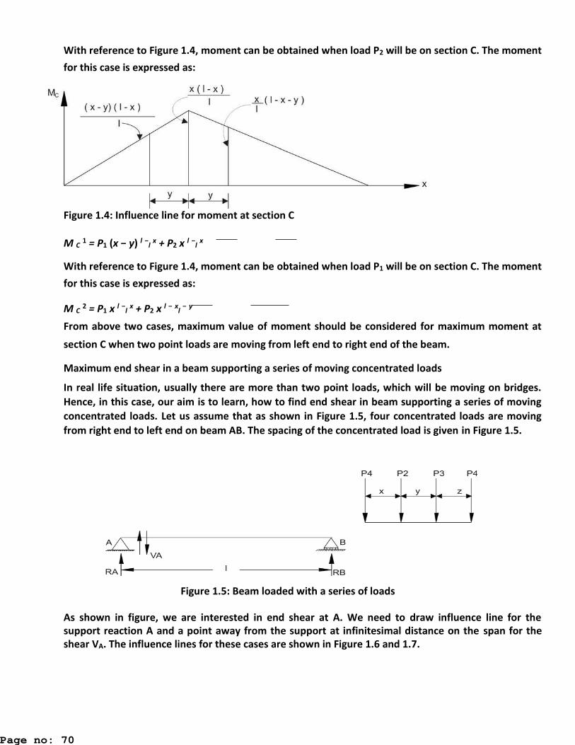
With reference to Figure 1.4, moment can be obtained when load P2 will be on section C. The moment

for this case is expressed as:

Figure 1.4: Influence line for moment at section C

M C 1 = P1 (x − y) l −l x + P2 x l −l x With reference to Figure 1.4, moment can be obtained when load P1 will be on section C. The moment

for this case is expressed as: M C 2 = P1 x l −l x + P2 x l − xl − y

From above two cases, maximum value of moment should be considered for maximum moment at

section C when two point loads are moving from left end to right end of the beam. Maximum end shear in a beam supporting a series of moving concentrated loads In real life situation, usually there are more than two point loads, which will be moving on bridges.

Hence, in this case, our aim is to learn, how to find end shear in beam supporting a series of moving

concentrated loads. Let us assume that as shown in Figure 1.5, four concentrated loads are moving

from right end to left end on beam AB. The spacing of the concentrated load is given in Figure 1.5.

Figure 1.5: Beam loaded with a series of loads As shown in figure, we are interested in end shear at A. We need to draw influence line for the support reaction A and a point away from the support at infinitesimal distance on the span for the shear VA. The influence lines for these cases are shown in Figure 1.6 and 1.7.

Page no: 70

Figure 1.6: Influence line for reaction at support A Figure 1.7: Influence line for shear near to support A. When loads are moving from B to A then as they move closer to A, the shear value will increase.

When load passes the support, there could be increase or decrease in shear value depending upon the next point load approaching support A. Using this simple logical approach, we will find out the change in shear value near support and monitor this change from positive value to negative value. He e fo the p ese t ase let us assu e that ΣP is su atio of the loads e ai i g o the ea . When load P1 crosses support A, then P2 will approach A. In that case, change in shear will be expressed as dV = ∑l

Px − P1 When load P2 crosses support A, then P3 will approach A. In that case change in shear will be

expressed as dV = ∑l

Py − P2 In case if dV is positive then shear at A has increased and if dV is negative, then shear at A has

decreased. Therefore, first load, which crosses and induces negative changes in shear, should be

placed on support A. Numerical Example Compute maximum end shear for the given beam loaded with moving loads as shown in Figure 1.8.

Page no: 71

When first load of 4 kN crosses support A and second load 8 kN is approaching support A, then

change in shear can be given by dV = ∑(8 +8 + 4)2 − 4 = 0 10 When second load of 8 kN crosses support A and third load 8 kN is approaching support A, then

change in shear can be given by dV = ∑(8 + 4)3 −8 = − . 10

Hence, as discussed earlier, the second load 8 kN has to be placed on support A to find out maximum

end shear (refer Figure 1.9).

Figure 1.9: Influence line for shear at A. VA = 4 ×1 +8 ×0.8 +8 ×0.5 + 4 ×0.3 =15.6kN Maximum shear at a section in a beam supporting a series of moving concentrated loads In this section we will discuss about the case, when a series of concentrated loads are moving on

beam and we are interested to find maximum shear at a section. Let us assume that series of loads

are moving from right end to left end as shown in Figure. 1.10.

Figure 1.10: Beam loaded with a series of loads

Page no: 72

Monitor the sign of change in shear at the section from positive to negative and apply the concept

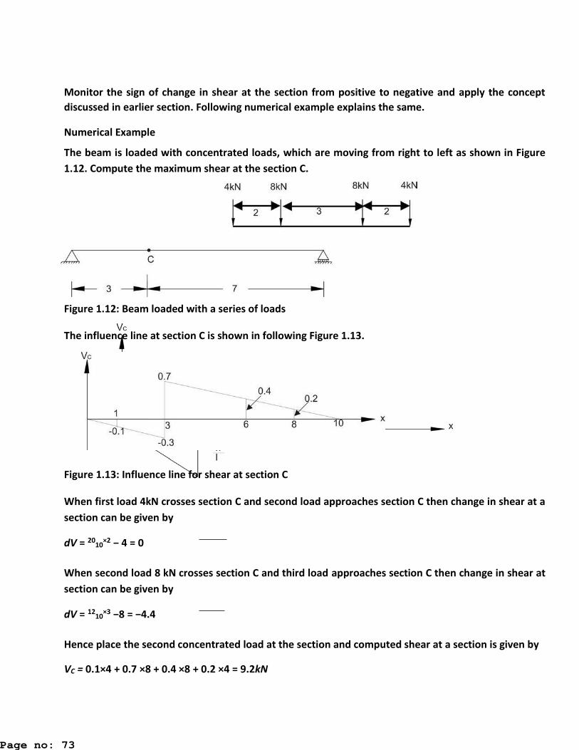
discussed in earlier section. Following numerical example explains the same. Numerical Example The beam is loaded with concentrated loads, which are moving from right to left as shown in Figure

1.12. Compute the maximum shear at the section C. Figure 1.12: Beam loaded with a series of loads The influence line at section C is shown in following Figure 1.13.

Figure 1.13: Influence line for shear at section C When first load 4kN crosses section C and second load approaches section C then change in shear at a

section can be given by dV = 20

10×2 − 4 = 0

When second load 8 kN crosses section C and third load approaches section C then change in shear at

section can be given by dV = 12

10×3 −8 = − .

Hence place the second concentrated load at the section and computed shear at a section is given by VC = 0.1×4 + 0.7 ×8 + 0.4 ×8 + 0.2 ×4 = 9.2kN

Page no: 73

Maximum Moment at a section in a beam supporting a series of moving concentrated loads The approach that we discussed earlier can be applied in the present context also to determine the maximum positive moment for the beam supporting a series of moving concentrated loads. The change in moment for a load P1 that moves from position x1 to x2 over a beam can be obtained by multiplying P1 by the change in ordinate of the influence line i.e. (y2 – y1). Let us assume the slope of the influence line (Figure 1.14) is S, then (y2 – y1) = S (x2 – x1).

Figure 1.14: Beam and Influence line for moment at section C Hence change in moment can be given by dM = P1S(x2 − x1) Let us consider the numerical example for better understanding of the developed concept.

Page no: 74