SUBGRID PARAMETERIZATION OF SNOW DISTRIBUTION FOR AN ENERGY AND

MASS BALANCE SNOW COVER MODEL

CHARLES H. LUCEUSDA Forest Service, Rocky Mtn. Research Station, 316 E. Myrtle, Boise, Idaho 83702

DAVID G. TARBOTONCivil and Environmental Engineering, Utah State University, Logan, Utah 84322-4110

ANDKEITH R. COOLEY

USDA Agricultural Research Service, Northwest Watershed Research Center,800 Park Blvd., Plaza 4, Suite 105, Boise, Idaho 83712-7716

Paper presented at the International Conference on SNOW HYDROLOGY, 6-9 October 1998,Brownsville, Vermont. USA.

This is a preprint of an article published in Hydrological Processes, 13(12-13): 1921-1933,special issue from International Conference on Snow Hydrology, September 1999. Thepublished version is available online at http://www.interscience.wiley.com/ orhttp://www3.interscience.wiley.com/cgi-bin/fulltext?ID=64500506&PLACEBO=IE.pdf

Copyright © 1999 John Wiley & Sons, Ltd.

1

SUBGRID PARAMETERIZATION OF SNOW DISTRIBUTION FOR AN ENERGY AND MASS

BALANCE SNOW COVER MODEL

CHARLES H. LUCEUSDA Forest Service, Rocky Mtn. Research Station, 316 E. Myrtle, Boise, Idaho 83702

DAVID G. TARBOTONCivil and Environmental Engineering, Utah State University, Logan, Utah 84322-4110

ANDKEITH R. COOLEY

USDA Agricultural Research Service, Northwest Watershed Research Center,800 Park Blvd., Plaza 4, Suite 105, Boise, Idaho 83712-7716

ABSTRACT

Representation of sub-element scale variability in snow accumulation and ablation is increasingly recognized

as important in distributed hydrologic modeling. Representing sub-grid scale variability may be

accomplished through numerical integration of a nested grid or through a lumped modeling approach. We

present a physically based model of the lumped snowpack mass and energy balance applied to a 26-ha

rangeland catchment with high spatial variability in snow accumulation and melt. Model state variables are

snow-covered area average snow energy content (U), the basin-average snow water equivalence (Wa), and

snow-covered area fraction (Af). The energy state variable is evolved through an energy balance. The snow

water equivalence state variable is evolved through a mass balance, and the area state variable is updated

according to an empirically derived relationship, Af(Wa), that is similar in nature to depletion curves used in

existing empirical basin snowmelt models. As snow accumulates, the snow covered area increases rapidly.

As the snowpack ablates, Af decreases as Wa decreases. This paper shows how the relationship Af(Wa) for the

melt season can be estimated from the distribution of snow water equivalence at peak accumulation in the area

being modeled. We show that the depletion curve estimated from the snow distribution of peak accumulation

2

at the Upper Sheep Creek sub-basin of Reynolds Creek Experimental Watershed compares well against the

observed depletion data as well as modeled depletion data from an explicit spatially distributed energy

balance model. Comparisons of basin average snow water equivalence between the lumped model and

spatially distributed model show good agreement. Comparisons to observed snow water equivalence show

poorer but still reasonable agreement. The sub-grid parameterization is easily portable to other physically

based point snowmelt models. It has potential application for use in hydrologic and climate models covering

large areas with large model elements, where a computationally inexpensive parameterization of sub-grid

snow processes may be important.

INTRODUCTION

Within the last 20 years, interest in scaling has increased within the hydrologic research community. The

increase in interest has been driven in part by a desire to apply physically based hydrologic models to

catchments and global circulation model (GCM) grid cells. Snowmelt has been an important hydrologic

process examined with respect to scaling. In mountainous regions, snowmelt is one of the largest surface

water inputs controlling runoff. Snow cover affects the atmosphere through its strong influence on the surface

radiation and energy balance.

At the catchment and GCM scale, interest lies in determining the effects of changing land use. Some of the

interest of atmospheric modelers relates to the effects of changing climate. Therefore, empirical hydrologic

models, may not be useful at these larger scales (Seyfried and Wilcox, 1995). Empirical models require

calibration under particular conditions. If land use or general climate conditions change, the correlations may

not necessarily be the same. Physically based models use parameters that are, at least in principle, related to

physical conditions and can sometimes be measured.

3

Physically based models tend to have a foundation in point-scale research. Much research of snowmelt

processes has been conducted at the plot or point scale (Hathaway et al., 1956; Anderson, 1976; Morris, 1986;

Morris, 1990; Jordan, 1991; Tarboton et al., 1995; Tarboton and Luce, 1997). Point scale models are often

not applicable for larger areas even using effective parameters calibrated for the catchment (Arola and

Lettenmaier, 1995; Luce et al., 1997, 1998). Snowmelt shares this characteristic with other hydrologic

processes (Beven, 1995, Kalma and Sivapalan, 1995). Generalized solutions available to solve the problem

are numerical integration (Abbot and Refsgaard, 1996), spatial distribution functions (Moore, 1985), and

parameterizations (Beven, 1995; Blöschl, 1996).

For snowmelt, several solutions have been applied. Numerical integration has been and continues to be a

popular method through use of distributed hydrologic models (Blöschl et al., 1991; Wigmosta et al., 1994;

Kirnbauer et al., 1994; Liston, 1997). The distribution function approach has also been applied to create

lumped models (Horne and Kavvas, 1997; Anderson, 1973; Rango and Van Katwijk, 1990; Martinec et al.,

1994). The areal depletion curve concept, which amounts to a distribution function approach, has been applied

to empirical models including the National Weather Service River Forecasting System (NWSRFS) and the

Snowmelt Runoff Model (Martinec et al., 1994). This approach can be adopted into a physically based

modeling framework by developing a relationship between the state variable of interest, snow water

equivalence over the basin, and the areal extent of snowcover. This is similar to the approach of

TOPMODEL (Beven and Kirkby, 1979) where saturated area is estimated as a function of the basin-averaged

stored water. In TOPMODEL, the parameterization relating the stored water state variable to the saturated

area is derived based on an analysis of the topography. With the lumped snowmelt model, the

parameterization relating the basin averaged snow water equivalence state variable to the fractional snow

4

coverage is derived based on a probability distribution/density function (pdf) of peak snow water equivalence.

Other remote sensing and modeling tools (Elder et al., 1989, 1991, 1995, 1998; Elder, 1995; Rosenthal and

Dozier, 1996) may be used to relate topography to the pdf of peak snow water equivalence.

The objectives of this paper are to present and test a physically based lumped model of snowpack evolution

for a small watershed (26 ha) that uses a depletion curve parameterization to relate the basin-averaged snow

water equivalence to snow-covered area. A secondary purpose is to present a method for deriving the

depletion curve from snowpack measurements at peak accumulation. This is part of an ongoing effort to

extend physically based modeling methodology to larger scales where it is impractical to apply a point model

over a grid of model elements small enough to ignore subgrid variability.

METHODS

The basic approach of this study compared the outputs of the lumped model to outputs from a distributed

snowmelt model and a series of distributed snow water equivalence observations. The lumped model treats

the study area (26 ha) as a single model element with subgrid variability parameterized through a depletion

curve. The distributed model was applied at a 30 m grid scale ignoring only subgrid variability smaller than

this scale and amounts to a numerical integration of the spatially distributed processes that are parameterized

in the lumped model. The depletion curve parameterization used for the lumped simulation was derived from

observations of the snow water equivalence pattern near the time of peak accumulation. This depletion curve

was compared to that derived from the series of distributed observations and from the output of the distributed

model.

5

Study Area and Observations

Snow survey and climatological data from the Upper Sheep Creek subbasin of the Reynolds Creek

Experimental Watershed in southwestern Idaho (Figure 1) form the observational basis of this study. The

Upper Sheep Creek watershed has an area of 26 ha and ranges between 1840 and 2040 m elevation (Figure 2).

Low sagebrush (Artemisia arbuscula Nutt.) communities cover the northeast portion of the basin, and big

sagebrush (Artemisia tridentata Nutt.) communities cover much of the southwestern half of the basin. Aspen

(Populus tremuloides Michx.) grow in a narrow strip along the northeast-facing slope where snow drifts

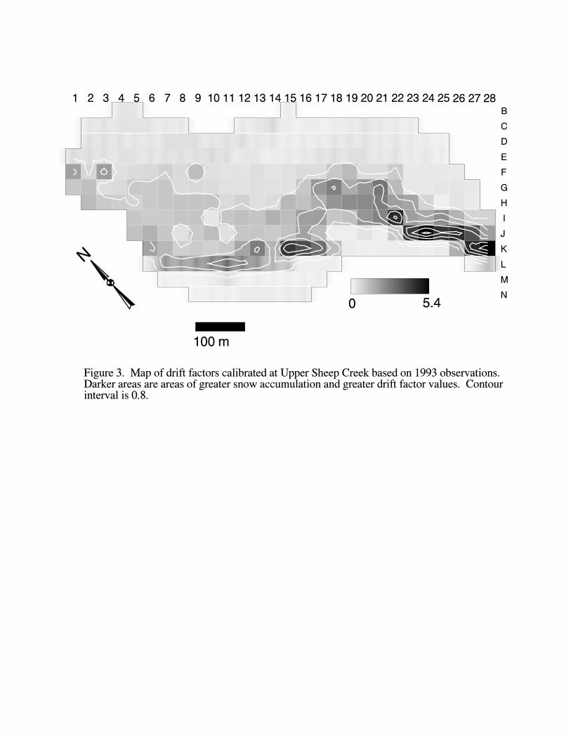
typically form (Figure 3). Severe winter weather and winds prevent the aspen from growing to heights greater

than 4-7 m. Average annual precipitation is 508 mm, and the first-order stream exiting the basin is ephemeral.

Upper Sheep Creek has been the site of many previous hydrologic investigations (Stephenson and Freeze,

1974; Cooley, 1988; Duffy et al., 1991; Flerchinger et al., 1992, 1994; Jackson, 1994; Seyfried and Wilcox,

1995; Tarboton et al., 1995; Luce et al., 1997, 1998; among others). Runoff generation has been the focus of

much of the work, and all of the studies have noted the importance of the wind-induced snowdrift in the

southwest portion of the basin to the basin hydrology. Previous work (Luce et al., 1997, 1998) has shown that

snow drifting is the primary determinant of spatial variability of snow in this watershed, more important than

topographically induced variations of radiation. Previous work measuring snow drifting (Cooley, 1988) and

distributed snowmelt modeling (Jackson, 1994; Tarboton et al., 1995; Luce et al., 1997, 1998) has provided

both foundation and incentive for development of a lumped snowmelt model of the basin that parameterizes

the subgrid variability due to snow drifting and spatially variable radiation processes.

The data used in this paper comprise measurements of snow water equivalence taken on nine dates in 1993

with a snow tube and scale. A systematic grid sampling strategy was used throughout the watershed (Figure

2). The grid spacing was 30.48 m (100 ft), and the long axis was oriented 48 degrees west of north.

6

Precipitation, temperature, relative humidity, and incoming solar radiation were measured for water year 1993

at a weather station near location J 10. Wind speed was measured at D 3.

Distributed Point Model

The distributed model is a cell-by-cell execution of the Utah Energy Balance (UEB) snowpack energy and

mass balance model (Tarboton et al., 1995; Tarboton and Luce, 1997). In order to run the model in a

distributed fashion, climatic inputs (radiation and precipitation) were calculated individually for each cell

based on measurements from the weather station, topography, and a calibrated drift factor.

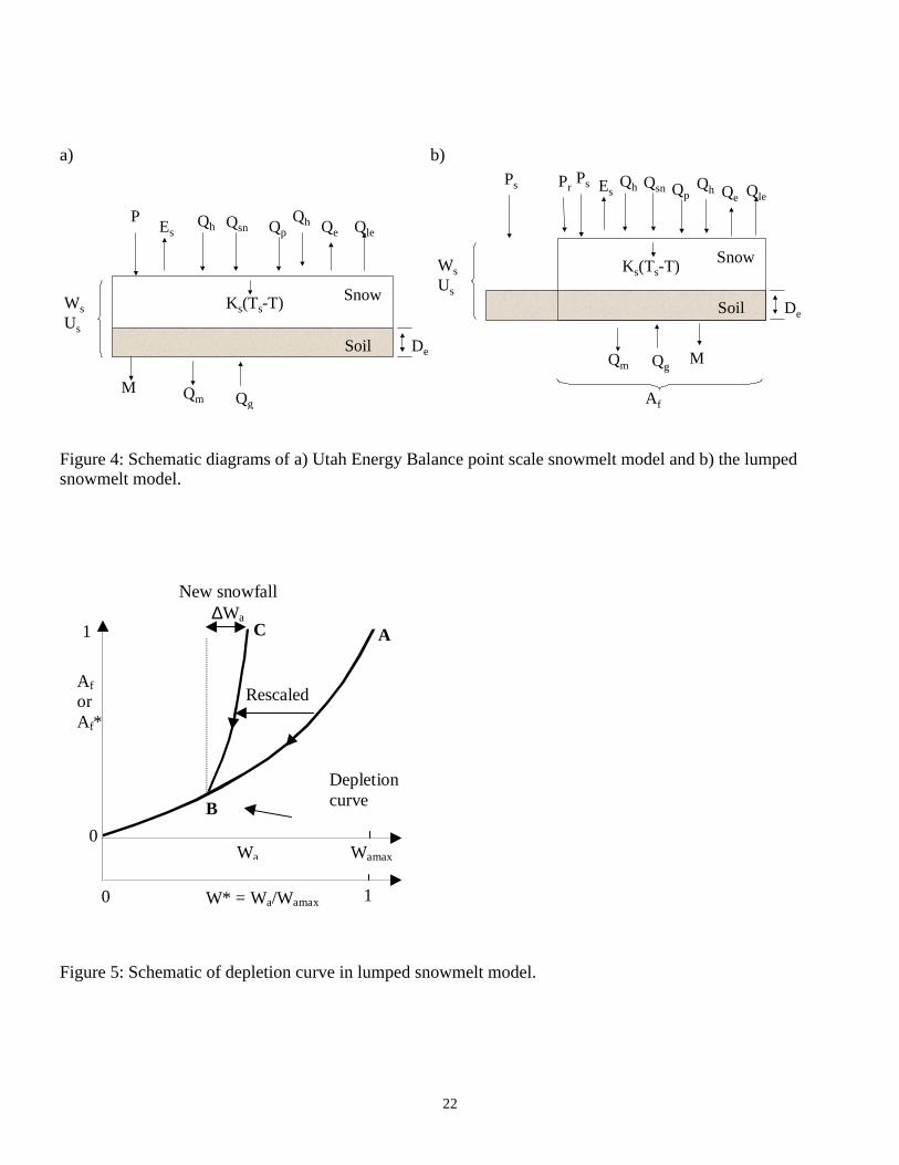
UEB is an energy and mass balance model with a vertically lumped representation of the snowpack. A

schematic is shown in Figure 4a. Two primary state variables are maintained in the model, snow water

equivalence, W [m], and internal energy of the snowpack and top 40 cm of soil, U [kJ m-2]. U is zero when

the snowpack is at 0° C and contains no liquid water. These two state variables are updated according to

dU/dt = Qsn+Qli-Qle+Qp+Qg+Qh+Qe-Qm (1)

dW/dt = Pr+Ps-Mr-E (2)

where Qsn is net solar radiation; Qli is incoming longwave radiation; Qle is outgoing longwave radiation; Qp is

advected heat from precipitation; Qg is ground heat flux; Qh is the sensible heat flux; Qe is the latent heat flux;

Qm is heat advected with melt water; Pr is the rate of precipitation as rain; Ps is the rate of precipitation as

snow; Mr is the melt rate; and E is the sublimation rate. The model is driven by inputs of precipitation, air

temperature, humidity, wind speed and incoming solar radiation. Snow surface temperature, a key variable in

calculating latent and sensible heat fluxes and outgoing longwave radiation, is calculated from the energy

7

balance at the surface of the snowpack, where incoming and outgoing fluxes must match. These simulations

were run on a 6-hr time step.

The effect of plant canopy on snowmelt is parameterized by decreasing the albedo of the snow surface as the

snow depth decreases below the canopy height. This parameterization is most appropriate for short

vegetation, such as sagebrush. Because the aspens are free of leaves until the soil warms slightly, errors

introduced by not considering the taller canopy are minimal.

The distributed model uses a drift multiplier to estimate enhancement of local incoming snow at each cell

through wind transport. The fraction of precipitation falling as rain or snow is a function of temperature. The

fraction of the gage catch falling as snow is multiplied by the drift multiplier to estimate grid cell

precipitation. The drift multiplier was calibrated at each grid cell to minimize the mean square error of the

point model relative to observations on February 10, March 3, and March 23, 1993. Values of the multiplier

over the basin are shown in Figure 3 and ranged from 0.16 to 5.36, with an average of 0.928.

Temporal variations in solar radiation were estimated based on an average atmospheric transmission factor

calculated from pyranometer data at the weather station. Local horizons, slope, and azimuth were used to find

local sunrise and sunset times and to integrate solar radiation received on the slope of each grid cell during

each time step. The calculated atmospheric transmission factor characterized cloudiness for incoming

longwave radiation calculations.

Lumped Model with Depletion Curve Parameterization

Figure 4b depicts schematically the lumped model with subgrid parameterization using depletion curves. This

is a modification of the UEB point-model (Figure 4a) described above. The snow-covered area fraction, Af, is

8

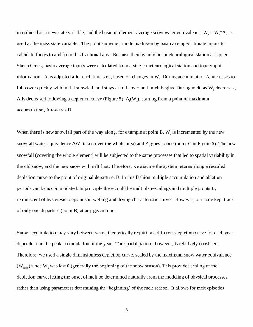
introduced as a new state variable, and the basin or element average snow water equivalence, Wa = Ws*A f, is

used as the mass state variable. The point snowmelt model is driven by basin averaged climate inputs to

calculate fluxes to and from this fractional area. Because there is only one meteorological station at Upper

Sheep Creek, basin average inputs were calculated from a single meteorological station and topographic

information. Af is adjusted after each time step, based on changes in Wa. During accumulation Af increases to

full cover quickly with initial snowfall, and stays at full cover until melt begins. During melt, as Wa decreases,

Af is decreased following a depletion curve (Figure 5), Af(Wa), starting from a point of maximum

accumulation, A towards B.

When there is new snowfall part of the way along, for example at point B, Wa is incremented by the new

snowfall water equivalence ∆W (taken over the whole area) and Af goes to one (point C in Figure 5). The new

snowfall (covering the whole element) will be subjected to the same processes that led to spatial variability in

the old snow, and the new snow will melt first. Therefore, we assume the system returns along a rescaled

depletion curve to the point of original departure, B. In this fashion multiple accumulation and ablation

periods can be accommodated. In principle there could be multiple rescalings and multiple points B,

reminiscent of hysteresis loops in soil wetting and drying characteristic curves. However, our code kept track

of only one departure (point B) at any given time.

Snow accumulation may vary between years, theoretically requiring a different depletion curve for each year

dependent on the peak accumulation of the year. The spatial pattern, however, is relatively consistent.

Therefore, we used a single dimensionless depletion curve, scaled by the maximum snow water equivalence

(Wamax) since Wa was last 0 (generally the beginning of the snow season). This provides scaling of the

depletion curve, letting the onset of melt be determined naturally from the modeling of physical processes,

rather than using parameters determining the ‘beginning’ of the melt season. It allows for melt episodes

9

during the accumulation season and accumulation episodes during the melt season. The following equation

gives a particular depletion curve, Af(Wa), in terms of the dimensionless depletion curve.

Af(Wa) = Af

*(Wa/Wamax) (3)

Snowfall inputs to the lumped model are adjusted by an element (basin) average drift factor to account for the

fact that even at the larger lumped model element scale, drifting and differences between the basin average

precipitation and gage precipitation may affect the net snow accumulation. In the results reported here the

basin average drift factor, 0.928, was used.

Depletion Curves

The depletion curve represents the functional decrease of snow-covered area fraction, Af, with decreasing

basin-average snow water equivalence, Wa, through the melt season. This can be viewed as a

parameterization of the distribution of snow over the basin. Note that this definition of a depletion curve

differs somewhat with the classical definition of Af as a function of melt, so requires some description on how

such curves may be estimated.

Spatial heterogeneity in snowpack water equivalence is linked to spatial variability in topography and

vegetation, which control relative accumulation and melt. Topography controls relative accumulation through

elevational temperature effects (precipitation as rain or snow) and drifting and controls melt through

elevational temperature effects and exposure to sunlight (Dozier, 1979; Dozier and Frew, 1990). Vegetation

controls accumulation through effects on drifting and interception and controls melt through effects on solar

radiation, wind, and temperature. The primary drivers in variability change with scale (Seyfried and Wilcox,

1995). Luce et al. (1997, 1998) found that the primary control on the spatial distribution of snow water

equivalence in Upper Sheep Creek was drifting. In larger basins, variations in wind, temperature, or solar

10

exposure could be important sources of variability in melt. Drifting exerts its influence during the

accumulation season. This suggests that the depletion curve for Upper Sheep Creek would be related to the

distribution of snow water equivalence during the peak accumulation.

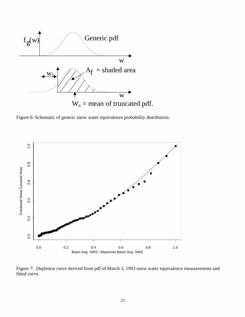
To formally develop this relationship, assume a generic probability distribution (pdf) for snow water

equivalence, fg(w), that retains a consistent shape through the melt season. The implication is spatially

uniform melt. This pdf gives the probability for point snow water equivalence areally sampled, offset by an

additive constant. As the snow accumulates and ablates this function shifts to the right or left. This procedure

is shown in Figure 6, and is conceptually similar to a procedure suggested in Dunne and Leopold (1978) but

generalized to non-Gaussian pdfs. The positioning of the generic pdf is controlled by the parameter w1, which

represents the amount of melt that has occurred. The tail to the left of the y-axis represents snow free area, for

any particular melt depth, w1. The snow-covered area fraction in terms of this pdf is defined as:

( ) ( ) ( ) )(1 1

0

11

1

wFdwwfdwwwfwA g

w

ggf −==+= ∫∫∞∞

(4)

where Fg(w1) is the cumulative density function evaluated at w1. For any arbitrary w1, Af(w1) is the fraction of

the basin with swe at peak accumulation greater than w1. Practically, the function, Af(w), may be numerically

evaluated directly from a sample of snow water equivalence values across the area of interest. (Note: This

function, Af(w) is not the same as the depletion curve, Af(Wa), the difference being indicated through a lower

case dummy argument, w or w1.)

The probability distribution of snow water equivalence for any particular w1 has a nugget at zero because a

negative swe has no physical interpretation. This nugget can be represented mathematically with a Dirac delta

function, so that the finite probability of the areally sampled snow water equivalence being zero is 1-Af(w1).

11

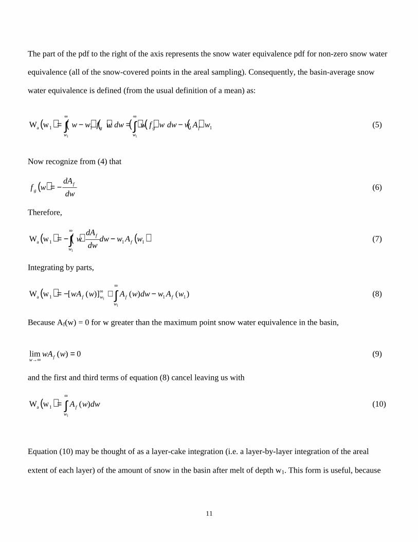
The part of the pdf to the right of the axis represents the snow water equivalence pdf for non-zero snow water

equivalence (all of the snow-covered points in the areal sampling). Consequently, the basin-average snow

water equivalence is defined (from the usual definition of a mean) as:

( ) ( ) ( ) ( ) ( ) ( )1111a

11

wW wAwdwwfwdwwfww fg

w

g

w

−=−= ∫∫∞∞

(5)

Now recognize from (4) that

( )dw

dAwf f

g −= (6)

Therefore,

( ) ( ) ( )111a

1

wW wAwdwdw

dAw f

w

f −−= ∫∞

(7)

Integrating by parts,

( ) )()()]([wW 111a

1

1wAwdwwAwwA f

w

fwf −+−= ∫∞

∞ (8)

Because Af(w) = 0 for w greater than the maximum point snow water equivalence in the basin,

0)(lim =∞→

wwAfw

(9)

and the first and third terms of equation (8) cancel leaving us with

( ) ∫∞

=1

)(wW 1a

w

f dwwA (10)

Equation (10) may be thought of as a layer-cake integration (i.e. a layer-by-layer integration of the areal

extent of each layer) of the amount of snow in the basin after melt of depth w1. This form is useful, because

12

Af(w) can be obtained easily from data. Numerical integration of Af(w) can be used to obtain Wa(w). Wamax is

Wa(w=0). The depletion curve, Af

*(Wa/Wamax), may be approximated by calculating Af(w) and Wa(w)/Wamax for

several values of w.

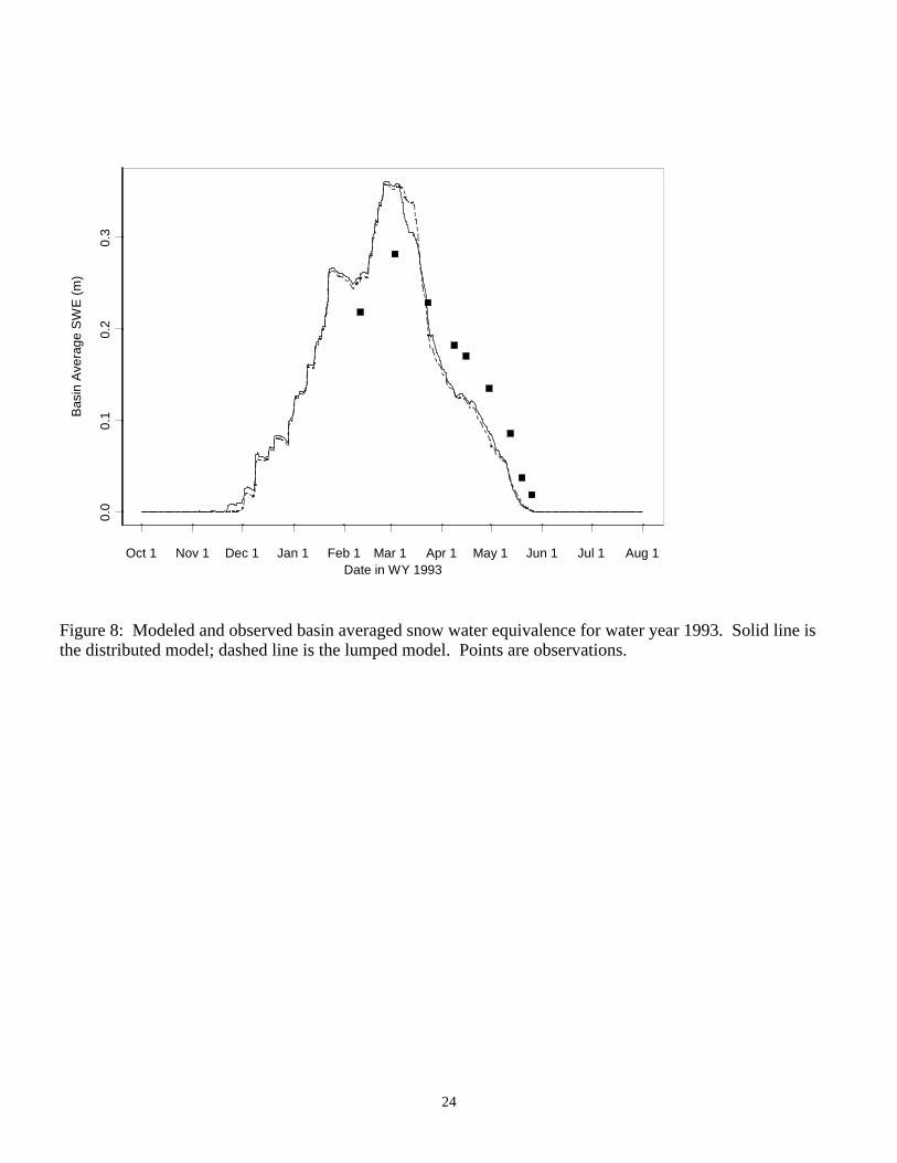
The pdf of snow water equivalence values sampled at peak snow accumulation define the pdf for all w1 ≥ 0.

Using the 254 sampled values of snow water equivalence from Upper Sheep Creek on March 3, 1993, Af(w1)

was calculated using equation 4 for w1 between 0 and the maximum observed snow water equivalence in steps

of 0.05 m. Wa(w1) was calculated for the same w1 values using equation 10. Af is plotted against Wa/Wamax in

Figure 7. A three-part curve was used to numerically encode this function.

( )

≤≤

≤≤−

≤≤

=

0.134.0 if

34.013.0 if 11.042.0

13.00 if 18.0

max5.1

max

maxmax

maxmax

aaaa

aaaa

aaaa

f

WWWW

WWWW

WWWW

A (11)

Af(Wa) was also found from the series of nine measurements and from the distributed model run for

comparison to the curve estimated from the peak accumulation pdf.

RESULTS AND DISCUSSION

A comparison between snow water equivalence predicted by the lumped and distributed models and measured

in the snow survey is presented in Figure 8. The lumped model matched the distributed model very well, but

both models overestimated the peak accumulation and showed a slightly early melt compared to observations.

The cell-by-cell calibration of the drift factor done using the February 10th, March 3rd, and March 23rd

observations gives some insight into the source of the error for the two models. Figure 9 shows an example of

13

the fit for two adjacent cells. One curve is a better fit to the data than the other and are typical of calibrations

obtained at other cells. Both modeled curves have a similar shape, dictated by the model physics and driving

climatic inputs. The differences between the model curves are based on one cell receiving greater modeled

snow precipitation than the other, as determined by the value of the drift multiplier, the only parameter

adjusted in the calibration. At some cells, the fit to the calibration period was good (e.g. L14) and at others, it

was poor (e.g. K14). In almost all cells with a poor fit, the pattern was similar to that at K14 (i.e.

overprediction of the peak accumulation). Both modeled curves predict early melt. The sum of many cells

with this pattern of overprediction and underprediction is an identical pattern of overprediction and

underprediction of the average (Figure 8).

In this study we used the Utah Energy Balance Model with the intent of having only the drift factor as an

adjustable parameter. All other parameters were set based on literature or calibration to a few sites (Tarboton

and Luce, 1997). From this basis, it could be said that the remaining differences between the observation and

point model estimates indicate problems with the point model. It is possible that these errors could be

rectified by making changes to the point model, but the emphasis of this paper is not incrementally improving

point models, rather it is the development of the distribution function approach which could be used with any

point model (e.g. Anderson, 1976; Jordan, 1991).

With one adjustable parameter in the point model, there are theoretically 255 adjustable parameters for the

basin, corresponding to each grid cell. However, our experience shows that the fundamental shape of the

snow water equivalence graph over time is affected little by the drift factor. This means that for the

aggregated distributed simulation there is really only one adjustable parameter, the average drift factor.

Simulating over 255 cells provides a pdf of snow water equivalence over the basin, and distributed solar

14

inputs. Luce et al. (1997, 1998) showed that the distributed solar information is of lesser value for this basin.

Thus the fundamental information used by the distributed model is the same information used by the lumped

model, a mean “drift factor” and a pdf of relative snow accumulation. When seen in this light, the close

agreement between the two models is not surprising.

Beven (1996) suggests that distributed models have too many degrees of freedom to be properly calibrated.

Indeed, it may be possible that the 255 values of drift factor could have been manipulated together to provide

a much better fit of the basin averaged snow water equivalence. However, when the distributed model is

constrained to match the values at each cell, the aggregated distributed model results are the same as a lumped

model using the probability density function information. This supports the idea that processes that can be

modeled in a distributed fashion with independence from cell to cell may also be efficiently modeled using a

lumped model that relates a probability density function of important site characteristics to important lumped

state variables.

A comparison of the dimensionless depletion curves derived from the pdf of peak snowpack accumulation,

the distributed model run, and the nine observations is shown in Figure 10. This figure shows that the

depletion curve derived from the pdf of snow water equivalence at the date of maximum accumulation (March

3) is a good approximation to the observed and distributed model estimates of the actual depletion curve.

This finding improves the utility of the depletion curve concept because detailed observations of snow water

equivalence over a basin at multiple times are unusual. Such observations would be necessary to either

directly estimate the depletion curve or calibrate a distributed model. One may protest that gridded

observations of snow water equivalence over a basin during peak accumulation are also rare. Tools have been

15

developed (Elder et al., 1989, 1991, 1995, 1998; Elder, 1995; Rosenthal and Dozier, 1996) to use remote

sensing and modeling to estimate the distribution of peak snowpacks. These tools and data are comparatively

inexpensive and provide a practical means to generate a depletion curve for the lumped model.

CONCLUSIONS

Through the use of an areal depletion curve it is possible to obtain lumped snowmelt model simulations that

agree well with distributed model results and observed data. We have also presented a new method for the

derivation of areal depletion curves from the distribution of peak snow water equivalence, and shown that the

areal depletion curve obtained using this method compares well with the actual and modeled (using a detailed

distributed model) areal depletion of snow. The finding suggests that the lumped model formulation applied

here is a good substitute for the distributed model when detailed spatial patterns are not required. The

distributed model required 255 simulations using the UEB model for each time step where the lumped model

required only one, demonstrating considerable savings in computational effort. Effort in determining

distributed parameters is likewise reduced.

The reasoning behind the model should work with any point energy balance model. From the point by point

calibration work, it was clear that the Utah Energy Balance model (Tarboton and Luce, 1997) did not always

match the point scale data well. It is possible that both the distributed results and basin average results could

be improved with a more detailed energy balance model.

Comparison of the depletion curve derived from the probability density function of peak snow accumulation

to the observed depletion curve and that produced by the distributed model are encouraging. This finding

combined with tools to quantify the distribution of snow over basins based on topography or remote sensing

16

gives the lumped modeling approach presented here potential practical utility. This finding may also be

useful for lumped empirical models that use the depletion curve concept.

REFERENCES

Abbot, M.B. and J.C. Refsgaard, (eds.) 1996. Distributed Hydrological Modeling. Kluwer Academic

Publishers, Netherlands.

Anderson, E. A. 1973. National Weather Service River Forecast System-Snow Accumulation and Ablation

Model. NOAA Technical Memorandum NWS HYDRO-17, U.S. Dept. of Commerce, Silver Spring,

Maryland.

Anderson, E. A. 1976. A Point Energy and Mass Balance Model of a Snow Cover. NOAA Technical Report

NWS 19, U.S. Dept. of Commerce. Silver Spring, Maryland. 150 pp.

Arola, A. and D.P. Lettenmaier. 1996. ‘Effects of subgrid spatial heterogeneity on GCM-Scale land surface

energy and moisture fluxes’, J. Climate 8: 1339-1349.

Beven, K.J. 1995. ‘Linking parameters Across Scales: Subgrid Parameterizations and Scale Dependent

Hydrological Models’, Chapter 15 in Scale Issues in Hydrological Modelling, J. D. Kalma and M. Sivapalan

(eds.), Wiley, Chichester, pp.263-281.

Beven, K. J. 1996. ‘A discussion of distributed hydrological modelling.’ In: M. B. Abbott and J. C. Refsgaard

(eds.), Distributed Hydrological Modelling. Kluwer Academic Publishers, Netherlands. pp. 255-278.

Beven, K.J. and M.J. Kirkby. 1979. ‘A physically based contributing area model of basin hydrology’,

Hydrological Sciences Bulletin, 24(1):43-69.

Blöschl, G. 1996. Scale and Scaling in Hydrology. Wiener Mitteilungen, Vienna, Austria. 346 pp.

Blöschl, G., D. Gutknecht, and R. Kirnbauer. 1991. ‘Distributed snowmelt simulations in an alpine catchment.

2. Parameter study and model predictions’. Water Resources Research, 27(12): 3181-3188.

Cooley, K. R. 1988. ‘Snowpack variability on western rangelands’. In Western Snow Conference

Proceedings, Kalispell, Montana, April 18-20.

17

Dozier, J. and J. Frew. 1990. ‘Rapid Calculation of Terrain Parameters for Radiation Modeling From Digital

Elevation Data’, IEEE Transactions on Geoscience and Remote Sensing, 28(5): 963-969.

Dozier, J. 1979. ‘A Solar Radiation Model for a Snow Surface in Mountainous Terrain’. In Proceedings

Modeling Snow Cover Runoff, S. C. Colbeck and M. Ray (eds.), U.S. Army Cold Reg. Res. Eng. Lab.,

Hanover, NH, pp.144-153.

Duffy, C.J., K.R. Cooley, N. Mock, and D. Lee. 1991. ‘Self-affine scaling and subsurface response to

snowmelt in steep terrain’, Journal of Hydrology, 123, 395-414.

Dunne, T. and L.B. Leopold. 1978. Water in Environmental Planning. W.H. Freeman and company, New

York, New York. 817 pp.

Elder, K. 1995. Snow Distribution in Alpine Watersheds, Ph.D Thesis, University of California, Santa

Barbara, California. 309 pp.

Elder, K. J., J. Dozier, and J. Michaelsen. 1989. ‘Spatial and temporal variation of net snow accumulationn in

a small alpine watershed, Emerald Lake basin, Sierra Nevada, California, U.S.A.’ Annals of Glaciology,

13:56-63.

Elder, K. J., J. Dozier, and J. Michaelsen. 1991. ‘Snow accumulation and distribution in an alpine watershed’,

Water Resources Research 27(7):1541-1552.

Elder, K., J. Michaelsen and J. Dozier. 1995. ‘Small basin Modeling of Snow Water Equivalence Using

Binary Regression Tree Methods’, Biogeochemistry of Seasonally Snow-Covered Catchments, K. A.

Tonnessen et al. (eds.), Proceedings of a Boulder Symposium, July 3-14, IAHS Publ. no. 228, pp.129-139.

Elder, K., W. Rosenthal and R. Davis. (1998). ‘Estimating the spatial distribution of snow water equivalence

in a montane watershed’, Hydrological Processes.

Flerchinger, G.N., K.R. Cooley, and D.R. Ralston. 1992. ‘Groundwater response to snowmelt in a

mountainous watershed’, Journal of Hydrology, 133, 293-311.

Flerchinger, G. N., K. R. Cooley, C. L. Hanson, M. S. Seyfried, and J. R. Wight. 1994. ‘A lumped parameter

water balance of a semi-arid watershed’, American Society of Agricultural Engineering Paper No. 94-2133,

18

International Summer Meeting of the ASAE, June 19-22, Kansas City, Missouri. American Society of

Agricultural Engineering, St. Joseph, Michigan, USA.

Hathaway, G.A. et al. 1956. Snow Hydrology, Summary report of the Snow Investigations, U.S. Army Corps

of Engineers, North Pacific Division, Portland, Oregon. 546 pp.

Horne, F. E. and M. L. Kavvas. 1997. ‘Physics of the spatially averaged snowmelt process’, Journal of

Hydrology, 191: 179-207.

Jackson, T.H.R. 1994. A spatially distributed snowmelt-driven hydrologic model applied to Upper Sheep

Creek. Ph.D. Thesis. Utah State University, Logan, Utah.

Jordan, R. 1991. A one-dimensional temperature model for a snow cover, Technical documentation for

SNTHERM.89, Special Technical Report 91-16, US Army CRREL.

Kalma, J. D. and M. Sivapalan, (eds.) 1995. Scale Issues in Hydrological Modeling, Wiley, 489 p.

Kirnbauer, R., G. Blöschl, and D. Gutknecht. 1994. ‘Entering the era of distributed snow models’, Nordic

Hydrology, 25, 1-24.

Liston, G.E. 1997. ‘Modeling Subgrid-Scale Snow Distributions in Regional Atmospheric and Hydrologic

Models’, Eos, Transactions, American Geophysical Union, 78(46):F204, AGU Fall Meeting Suppl.

Luce, C. H., D. G. Tarboton and K. R. Cooley. 1997. Spatially Distributed Snowmelt Inputs to a Semi-Arid

Mountain Watershed. In Proceedings of the Western Snow Conference, Banff, Canada, May 5-8, 1997.

Luce, C.H., D.G. Tarboton and K.R. Cooley. (1998). ‘The influence of the spatial distribution of snow on

basin-averaged snowmelt’, Hydrological Processes.

Martinec, J., A. Rango and R. Roberts. 1994. The Snowmelt-Runoff Model (SRM) Users Manual, Updated

Edition 1994, Version 3.2, Department of Geography - University of Bern.

Moore, R. J. 1985. ‘The probability-distributed principle and runoff production at point and basin scales’,

Hydrological Sciences Journal, 30(2): 273-297.

Morris, E. M. (ed.). 1986. Modelling Snowmelt-Induced Processes, IAHS publication no. 155.

19

Morris, E. M. 1990. ‘Physics-Based Models of Snow’, In Recent Advances in the Modeling of Hydrologic

Systems, D.S. Bowles, and P.E. O’Connell (eds), Kluwer Academic Publishers, Dordrecht, The Netherlands.

pp. 85-112.

Rango, A. and V. Van Katwijk. 1990. ‘Development and testing of a snowmelt-runoff forecasting

technique’, Water Resources Bulletin, 25(1): 135-144.

Rosenthal, W. and J. Dozier. 1996. ‘Automated Mapping of Montane Snow Cover at Subpixel Resolution

from the Landsat Thematic Mapper’, Water Resources Research, 32(1): 115-130.

Seyfried, M. S. and B. P. Wilcox. 1995. ‘Scale and the nature of spatial variability: Field examples having

implications for hydrologic modeling.’ Water Resources Research, 31(1): 173-184.

Stephenson, G. R. and R. A. Freeze. 1974. ‘Mathematical simulation of subsurface flow contributions to

snowmelt runoff, Reynolds Creek watershed, Idaho’, Water Resources Research, 10(2): 284-294.

Tarboton, D. G. and C. H. Luce. 1997. Utah Energy Balance Snow Accumulation and Melt Model (UEB).

Computer model technical description and users guide. Utah Water Research Laboratory, Logan, Utah.

Tarboton, D.G., T. G. Chowdhury, and T. H. Jackson. 1995. ‘A spatially distributed energy balance

snowmelt model.’ Biogeochemistry of Seasonally Snow-Covered Catchments, K. A. Tonnessen et al. (eds.),

Proceedings of a Boulder Symposium, July 3-14, IAHS Publ. no. 228. pp. 141-155.

Wigmosta, M.S., L.W. Vail, and D.P. Lettenmaier. 1994. ‘A distributed hydrology-vegetation model for

complex terrain’, Water Resources Research, 30(6):1665-1679.

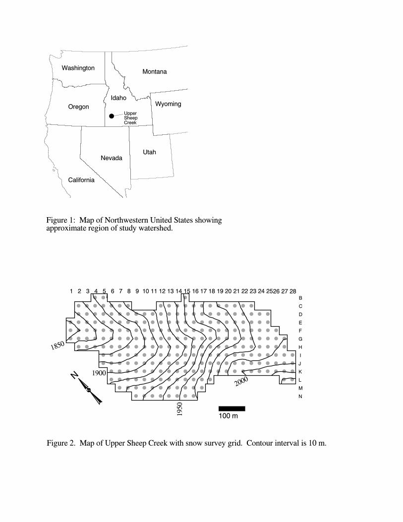
Figure 2. Map of Upper Sheep Creek with snow survey grid. Contour interval is 10 m.

2000

1950

1900

1850

N

100 m

# # ## # # # # # # # # # # # # # # # # # ## # # # # # # # # # # # # # # # # # # # # # # #

# # # # # # # # # # # # # # # # # # # # # # # # ## # # # # # # # # # # # # # # # # # # # # # # # # ## # # # # # # # # # # # # # # # # # # # # # # # # # #

# # # # # # # # # # # # # # # # # # # # # # # # # ## # # # # # # # # # # # # # # # # # # # # # # ## # # # # # # # # # # # # # # # # # # # # # # #

# # # # # # # # # # # # # # # # # # # # # # ## # # # # # # # # # # # # # #

# # # # # # # # # # ## # # # # # # #

C D E F

G H I J K L M N

B 1 2 3 4 5 6 7 8 9 10 11 12 13 14 15 16 17 18 19 20 21 22 23 24 25 26 27 28

Figure 1: Map of Northwestern United States showing approximate region of study watershed.

# UpperSheepCreek

Washington

Oregon

California

NevadaUtah

Idaho

Montana

Wyoming

100 m

Figure 3. Map of drift factors calibrated at Upper Sheep Creek based on 1993 observations. Darker areas are areas of greater snow accumulation and greater drift factor values. Contour interval is 0.8.

N

28 27 2625242322212019181716151413121110 9 8 7 6 5 4 3 2 1B

N

L K J I H

F E D C

G

M

0 5.4

22

a) b)

Snow

Soil De

Qsn Qp

Qm

Qh Qe QleP

M

Es

Ws

Us

Qg

Qh

Ks(Ts-T)

Snow

Soil De

Qsn Qp

Qm

Qh Qe Qle

Ps

M

Es

Ws

Us

Qg

Qh

Ks(Ts-T)

PsPr

Af

Figure 4: Schematic diagrams of a) Utah Energy Balance point scale snowmelt model and b) the lumpedsnowmelt model.

New snowfall∆Wa

Af

orAf*

0

1

10

Rescaled

W* = Wa/Wamax

Depletioncurve

Wamax

C A

B

Wa

Figure 5: Schematic of depletion curve in lumped snowmelt model.

23

Wa = mean of truncated pdf.

f (w)g

A = shaded areaf

Generic pdf

w1

w

w

Figure 6: Schematic of generic snow water equivalence probability distribution.

0.0 0.2 0.4 0.6 0.8 1.0

0.0

0.2

0.4

0.6

0.8

1.0

Basin Avg. SWE / Maximum Basin Avg. SWE

Fra

ctio

nal S

now

Cov

ered

Are

a

Figure 7: Depletion curve derived from pdf of March 3, 1993 snow water equivalence measurements andfitted curve.

24

Oct 1 Nov 1 Dec 1 Jan 1 Feb 1 Mar 1 Apr 1 May 1 Jun 1 Jul 1 Aug 1

0.0

0.1

0.2

0.3

Date in WY 1993

Bas

in A

vera

ge S

WE

(m

)

Figure 8: Modeled and observed basin averaged snow water equivalence for water year 1993. Solid line isthe distributed model; dashed line is the lumped model. Points are observations.

25

Oct 1 Nov 1 Dec 1 Jan 1 Feb 1 Mar 1 Apr 1 May 1 Jun 1 Jul 1 Aug 1

0.0

0.2

0.4

0.6

0.8

1.0

Date in WY 1993

Sno

w W

ater

Equ

ival

ence

(m

)

Figure 9: Plots of observed and modeled snow water equivalence at cells K14 (solid line and solid squares)and L14 (dashed line and open triangles). Model was calibrated by minimizing mean square error for the firstthree measurements of the year. The drift factor estimated for K14 is 2.55 and for L14 is 2.09. The solid lineis representative of locations where poor calibrations were obtained and the dashed line is representative oflocations where good calibrations were obtained.

26

0.0 0.2 0.4 0.6 0.8 1.0

0.0

0.2

0.4

0.6

0.8

1.0

Basin Avg. SWE / Maximum Basin Avg. SWE

Fra

ctio

nal S

now

Cov

ered

Are

a

Figure 10: Comparison of depletion curves derived from 1) pdf of March 3, 1993 snow survey (line), 2)distributed model output (gray circles), and 3) snow surveys taken on 9 dates (solid squares).