1

Spatial Analysis Exercise GIS in Water Resources

Fall 2013

Prepared by David G. Tarboton and David R. Maidment

Goal

The goal of this exercise is to serve as an introduction to Spatial Analysis with ArcGIS.

Objectives

• Calculate slope from a grid digital elevation model • Apply model builder geoprocessing capability to program a sequence of ArcGIS functions • Use ArcGIS.com services to access and extract elevation data • Use raster data and raster calculator functionality to calculate watershed attributes such as mean

elevation, mean annual precipitation and runoff ratio. • Interpolate data values at points to create a spatial field to use in hydrologic calculations

Computer and Data Requirements

To carry out this exercise, you need to have a computer, which runs ArcGIS for Desktop 10.2. The necessary data are provided in the accompanying zip file, http://www.neng.usu.edu/cee/faculty/dtarb/giswr/2013/Ex3Data.zip

Readings

Handout on "Computation of Slope" http://www.neng.usu.edu/cee/faculty/dtarb/giswr/2013/Slope.pdf

2

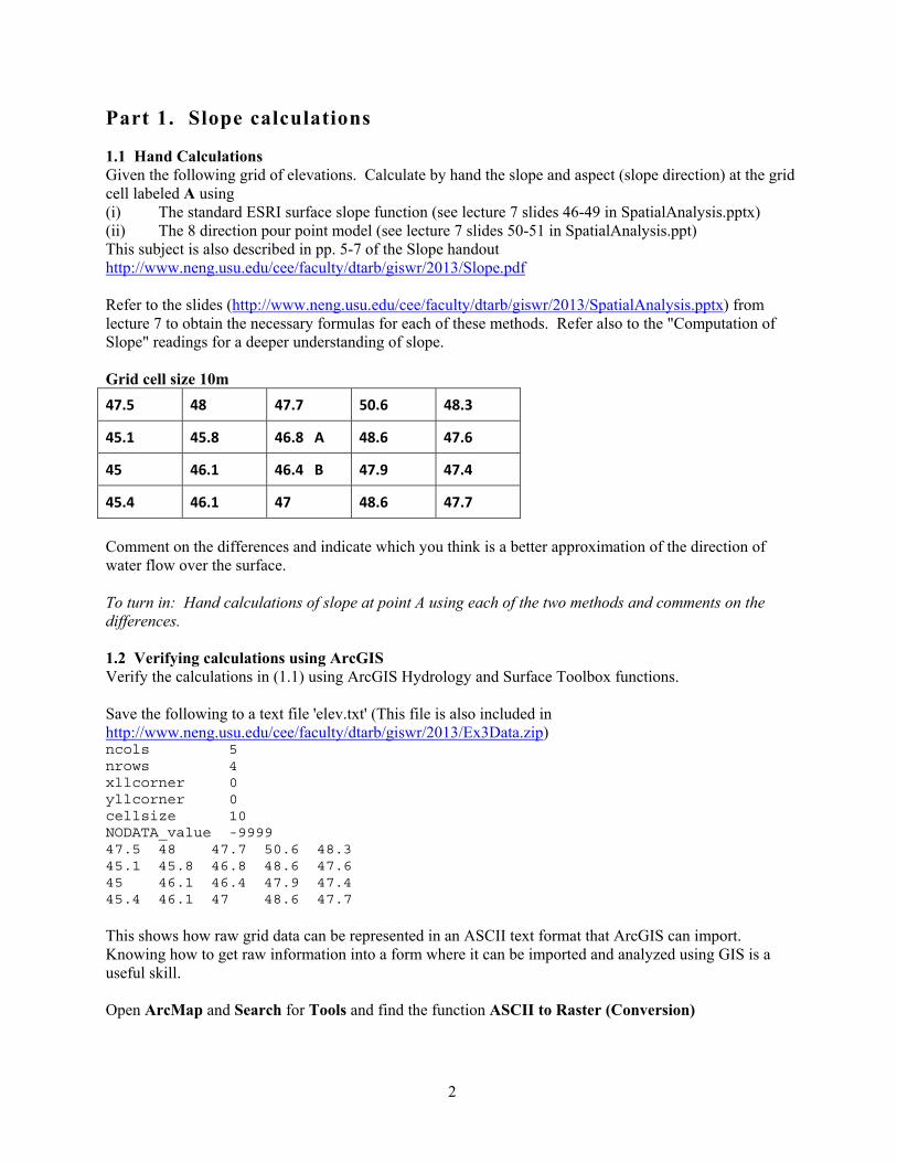
Part 1. Slope calculations

1.1 Hand Calculations Given the following grid of elevations. Calculate by hand the slope and aspect (slope direction) at the grid cell labeled A using (i) The standard ESRI surface slope function (see lecture 7 slides 46-49 in SpatialAnalysis.pptx) (ii) The 8 direction pour point model (see lecture 7 slides 50-51 in SpatialAnalysis.ppt) This subject is also described in pp. 5-7 of the Slope handout http://www.neng.usu.edu/cee/faculty/dtarb/giswr/2013/Slope.pdf Refer to the slides (http://www.neng.usu.edu/cee/faculty/dtarb/giswr/2013/SpatialAnalysis.pptx) from lecture 7 to obtain the necessary formulas for each of these methods. Refer also to the "Computation of Slope" readings for a deeper understanding of slope. Grid cell size 10m

47.5 48 47.7 50.6 48.3

45.1 45.8 46.8 A 48.6 47.6

45 46.1 46.4 B 47.9 47.4

45.4 46.1 47 48.6 47.7

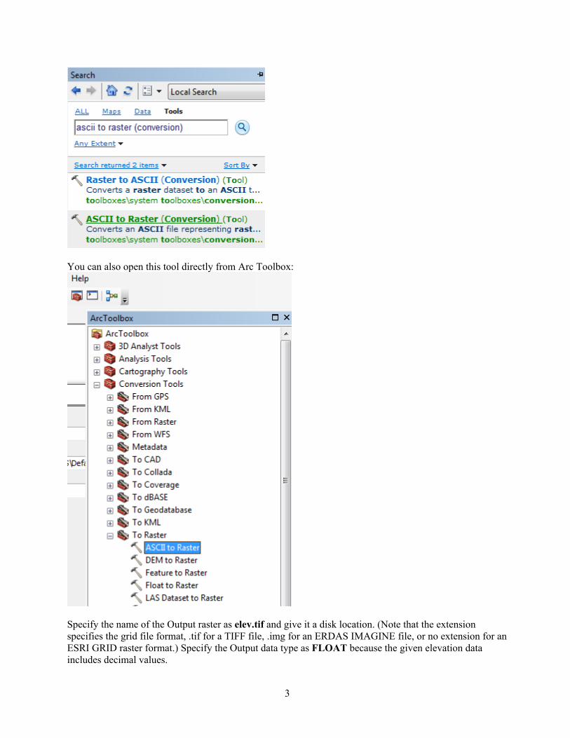
Comment on the differences and indicate which you think is a better approximation of the direction of water flow over the surface. To turn in: Hand calculations of slope at point A using each of the two methods and comments on the differences. 1.2 Verifying calculations using ArcGIS Verify the calculations in (1.1) using ArcGIS Hydrology and Surface Toolbox functions. Save the following to a text file 'elev.txt' (This file is also included in http://www.neng.usu.edu/cee/faculty/dtarb/giswr/2013/Ex3Data.zip) ncols 5 nrows 4 xllcorner 0 yllcorner 0 cellsize 10 NODATA_value -9999 47.5 48 47.7 50.6 48.3 45.1 45.8 46.8 48.6 47.6 45 46.1 46.4 47.9 47.4 45.4 46.1 47 48.6 47.7 This shows how raw grid data can be represented in an ASCII text format that ArcGIS can import. Knowing how to get raw information into a form where it can be imported and analyzed using GIS is a useful skill. Open ArcMap and Search for Tools and find the function ASCII to Raster (Conversion)

3

You can also open this tool directly from Arc Toolbox:

Specify the name of the Output raster as elev.tif and give it a disk location. (Note that the extension specifies the grid file format, .tif for a TIFF file, .img for an ERDAS IMAGINE file, or no extension for an ESRI GRID raster format.) Specify the Output data type as FLOAT because the given elevation data includes decimal values.

4

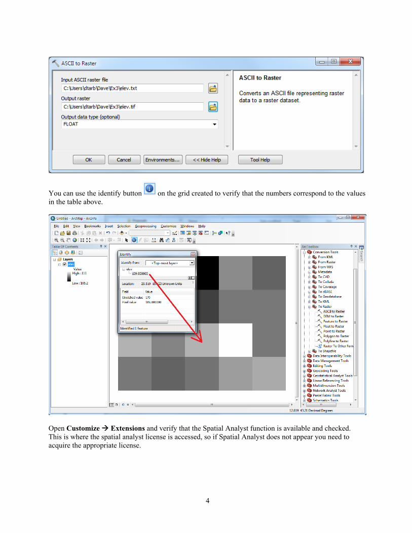
You can use the identify button on the grid created to verify that the numbers correspond to the values in the table above.

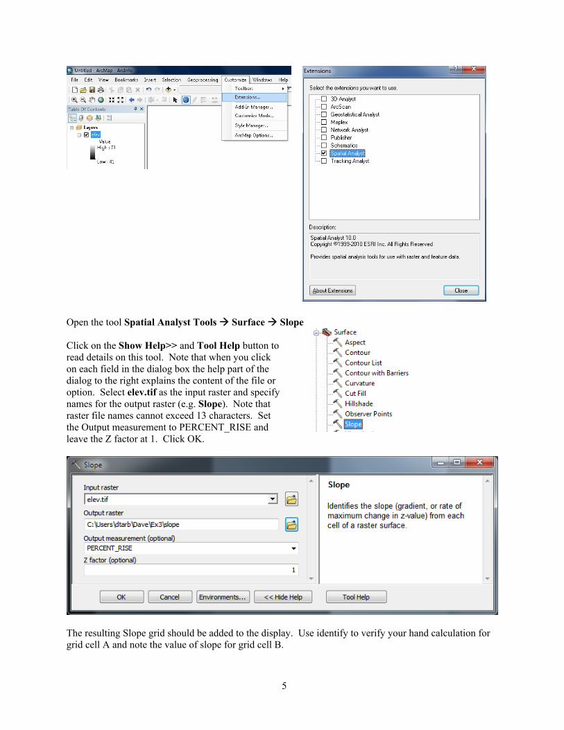
Open Customize Extensions and verify that the Spatial Analyst function is available and checked. This is where the spatial analyst license is accessed, so if Spatial Analyst does not appear you need to acquire the appropriate license.

5

Open the tool Spatial Analyst Tools Surface Slope Click on the Show Help>> and Tool Help button to read details on this tool. Note that when you click on each field in the dialog box the help part of the dialog to the right explains the content of the file or option. Select elev.tif as the input raster and specify names for the output raster (e.g. Slope). Note that raster file names cannot exceed 13 characters. Set the Output measurement to PERCENT_RISE and leave the Z factor at 1. Click OK.

The resulting Slope grid should be added to the display. Use identify to verify your hand calculation for grid cell A and note the value of slope for grid cell B.

6

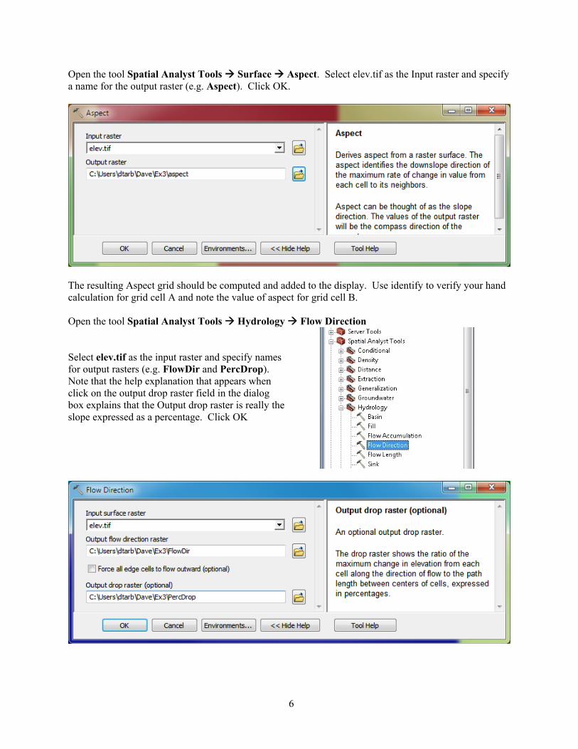
Open the tool Spatial Analyst Tools Surface Aspect. Select elev.tif as the Input raster and specify a name for the output raster (e.g. Aspect). Click OK.

The resulting Aspect grid should be computed and added to the display. Use identify to verify your hand calculation for grid cell A and note the value of aspect for grid cell B. Open the tool Spatial Analyst Tools Hydrology Flow Direction Select elev.tif as the input raster and specify names for output rasters (e.g. FlowDir and PercDrop). Note that the help explanation that appears when click on the output drop raster field in the dialog box explains that the Output drop raster is really the slope expressed as a percentage. Click OK

7

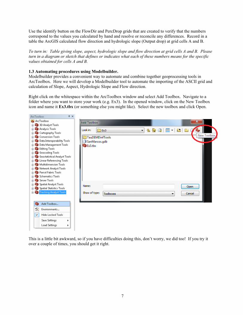
Use the identify button on the FlowDir and PercDrop grids that are created to verify that the numbers correspond to the values you calculated by hand and resolve or reconcile any differences. Record in a table the ArcGIS calculated flow direction and hydrologic slope (Output drop) at grid cells A and B. To turn in: Table giving slope, aspect, hydrologic slope and flow direction at grid cells A and B. Please turn in a diagram or sketch that defines or indicates what each of these numbers means for the specific values obtained for cells A and B. 1.3 Automating procedures using Modelbuilder. Modelbuilder provides a convenient way to automate and combine together geoprocessing tools in ArcToolbox. Here we will develop a Modelbuilder tool to automate the importing of the ASCII grid and calculation of Slope, Aspect, Hydrologic Slope and Flow direction. Right click on the whitespace within the ArcToolbox window and select Add Toolbox. Navigate to a folder where you want to store your work (e.g. Ex3). In the opened window, click on the New Toolbox icon and name it Ex3.tbx (or something else you might like). Select the new toolbox and click Open.

This is a little bit awkward, so if you have difficulties doing this, don’t worry, we did too! If you try it over a couple of times, you should get it right.

8

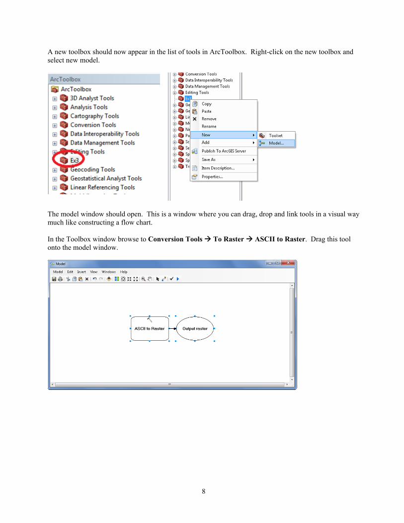
A new toolbox should now appear in the list of tools in ArcToolbox. Right-click on the new toolbox and select new model.

The model window should open. This is a window where you can drag, drop and link tools in a visual way much like constructing a flow chart. In the Toolbox window browse to Conversion Tools To Raster ASCII to Raster. Drag this tool onto the model window.

9

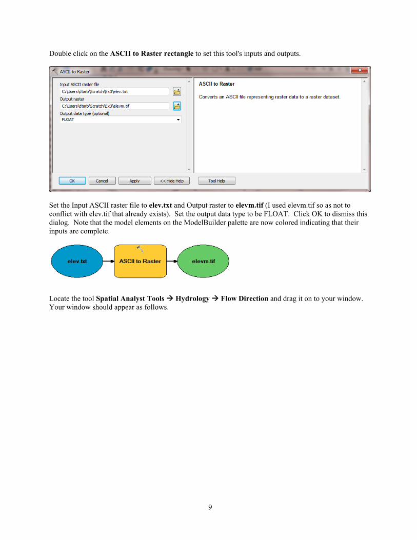
Double click on the ASCII to Raster rectangle to set this tool's inputs and outputs.

Set the Input ASCII raster file to elev.txt and Output raster to elevm.tif (I used elevm.tif so as not to conflict with elev.tif that already exists). Set the output data type to be FLOAT. Click OK to dismiss this dialog. Note that the model elements on the ModelBuilder palette are now colored indicating that their inputs are complete.

Locate the tool Spatial Analyst Tools Hydrology Flow Direction and drag it on to your window. Your window should appear as follows.

10

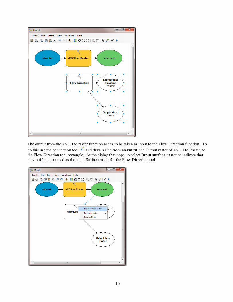
The output from the ASCII to raster function needs to be taken as input to the Flow Direction function. To

do this use the connection tool and draw a line from elevm.tif, the Output raster of ASCII to Raster, to the Flow Direction tool rectangle. At the dialog that pops up select Input surface raster to indicate that elevm.tif is to be used as the input Surface raster for the Flow Direction tool.

11

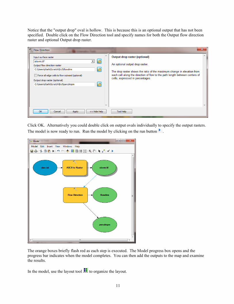
Notice that the "output drop" oval is hollow. This is because this is an optional output that has not been specified. Double click on the Flow Direction tool and specify names for both the Output flow direction raster and optional Output drop raster.

Click OK. Alternatively you could double click on output ovals individually to specify the output rasters.

The model is now ready to run. Run the model by clicking on the run button .

The orange boxes briefly flash red as each step is executed. The Model progress box opens and the progress bar indicates when the model completes. You can then add the outputs to the map and examine the results.

In the model, use the layout tool to organize the layout.

12

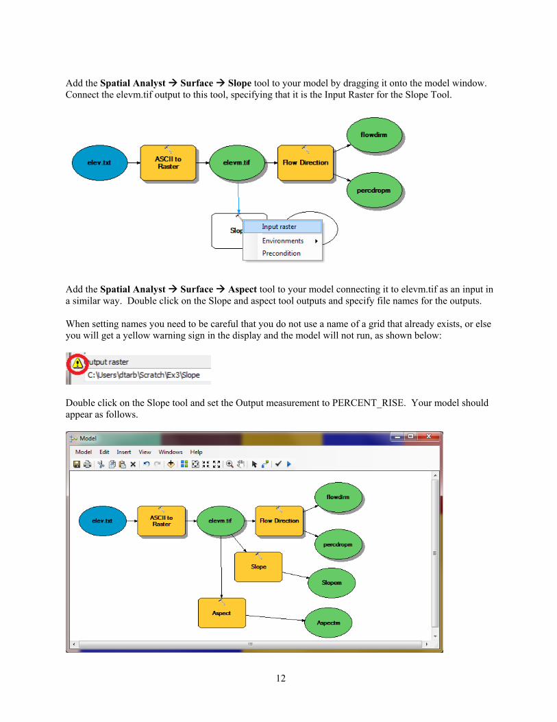
Add the Spatial Analyst Surface Slope tool to your model by dragging it onto the model window. Connect the elevm.tif output to this tool, specifying that it is the Input Raster for the Slope Tool.

Add the Spatial Analyst Surface Aspect tool to your model connecting it to elevm.tif as an input in a similar way. Double click on the Slope and aspect tool outputs and specify file names for the outputs. When setting names you need to be careful that you do not use a name of a grid that already exists, or else you will get a yellow warning sign in the display and the model will not run, as shown below:

Double click on the Slope tool and set the Output measurement to PERCENT_RISE. Your model should appear as follows.

13

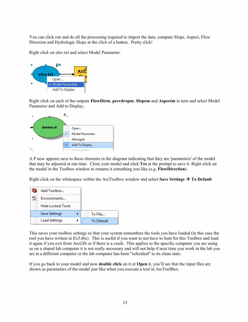
You can click run and do all the processing required to import the data, compute Slope, Aspect, Flow Direction and Hydrologic Slope at the click of a button. Pretty slick! Right click on elev.txt and select Model Parameter.

Right click on each of the outputs FlowDirm, percdropm, Slopem and Aspectm in turn and select Model Parameter and Add to Display.

A P now appears next to these elements in the diagram indicating that they are 'parameters' of the model that may be adjusted at run time. Close your model and click Yes at the prompt to save it. Right click on the model in the Toolbox window to rename it something you like (e.g. FlowDirection). Right click on the whitespace within the ArcToolbox window and select Save Settings To Default

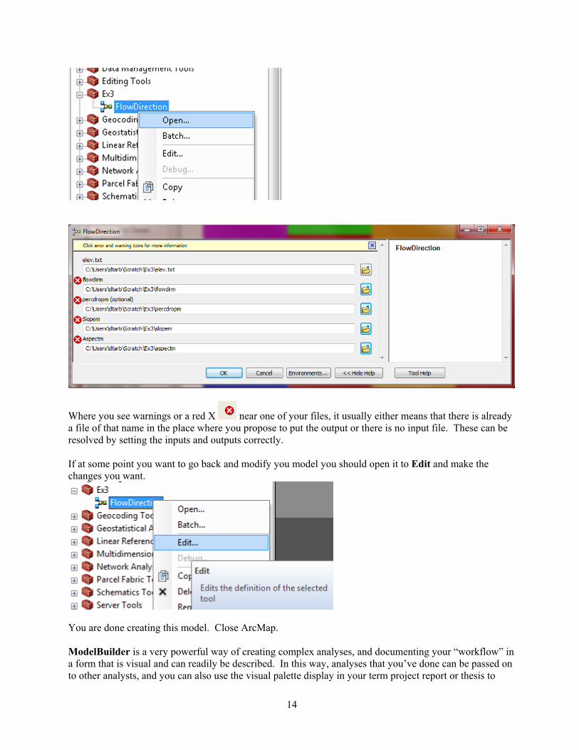
This saves your toolbox settings so that your system remembers the tools you have loaded (in this case the tool you have written in Ex3.tbx). This is useful if you want to not have to hunt for this Toolbox and load it again if you exit from ArcGIS or if there is a crash. This applies to the specific computer you are using so on a shared lab computer it is not really necessary and will not help if next time you work in the lab you are at a different computer or the lab computer has been "refreshed" to its clean state. If you go back to your model and now double click on it or Open it, you’ll see that the input files are shown as parameters of the model just like when you execute a tool in ArcToolBox.

14

Where you see warnings or a red X near one of your files, it usually either means that there is already a file of that name in the place where you propose to put the output or there is no input file. These can be resolved by setting the inputs and outputs correctly. If at some point you want to go back and modify you model you should open it to Edit and make the changes you want.

You are done creating this model. Close ArcMap. ModelBuilder is a very powerful way of creating complex analyses, and documenting your “workflow” in a form that is visual and can readily be described. In this way, analyses that you’ve done can be passed on to other analysts, and you can also use the visual palette display in your term project report or thesis to

15

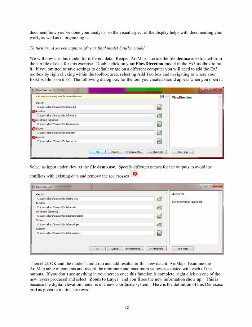
document how you’ve done your analysis, so the visual aspect of the display helps with documenting your work, as well as in organizing it. To turn in: A screen capture of your final model builder model. We will now use this model for different data. Reopen ArcMap. Locate the file demo.asc extracted from the zip file of data for this exercise. Double click on your FlowDirection model in the Ex3 toolbox to run it. If you omitted to save settings to default or are on a different computer you will need to add the Ex3 toolbox by right clicking within the toolbox area, selecting Add Toolbox and navigating to where your Ex3.tbx file is on disk. The following dialog box for the tool you created should appear when you open it.

Select as input under elev.txt the file demo.asc. Specify different names for the outputs to avoid the

conflicts with existing data and remove the red crosses .

Then click OK and the model should run and add results for this new data to ArcMap. Examine the ArcMap table of contents and record the minimum and maximum values associated with each of the outputs. If you don’t see anything in your screen once this function is complete, right click on one of the new layers produced and select “Zoom to Layer” and you’ll see the new information show up. This is because the digital elevation model is in a new coordinate system. Here is the definition of this Demo.asc grid as given in its first six rows:

16

ncols 296 nrows 233 xllcorner 2438224.25 yllcorner 5855081 cellsize 30 NODATA_value -9999 To turn in: A table giving the minimum and maximum values of each of the four outputs Slope, Aspect, Flow Direction, and Hydrologic Slope (Percentage drop), for the digital elevation model in demo.asc. Congratulations, you have just built a Model Builder geoprocessing program and used it to repeat your work for a different (and larger) dataset. If you would like to save this tool to take to another computer or share with someone else you can copy the file Ex3.tbx from its location to a removable media to take with you. If you are going to be sharing this tool more widely there are additional steps to take to clean up the interface (to avoid red X's), label the input fields and write help documentation for it. Close ArcMap.

Part 2. San Marcos Elevation and Precipitation.

The purpose of this part of the exercise is to calculate average watershed elevation for subwatersheds of the San Marcos basin, and to calculate average precipitation over each of these subwatersheds using different interpolation methods. The following data is provided in the Ex3Data.zip file. SanMarcos.gdb file Geodatabase.

There are the following feature classes:

- Basin. The San Marcos Basin feature class from exercise 2. - Gages. The San Marcos Gages from exercise 2 that includes Mean Annual Flow. - PrecipStn. PrecipStn contains mean annual precipitation data from precipitation stations in and

around the San Marcos basin downloaded from NCDC following the procedures given in http://www.ce.utexas.edu/prof/maidment/gradhydro2005/docs/ncdcdata.doc. (The NCDC website has changed so it is no longer possible to get this data this way) This data was prepared by downloading all years of available precipitation data for the counties in and around the San Marcos basin, then averaging over these years, retaining only those stations with 6 or more years of annual total data reported by NCDC.

- Subwatershed. Subwatersheds delineated to each of the stream gages used in exercise 2 following the procedures that will be learned in a future exercise.

1. Loading the Data

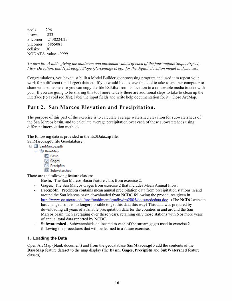
Open ArcMap (blank document) and from the geodatabase SanMarcos.gdb add the contents of the BaseMap feature dataset to the map display (the Basin, Gages, PrecipStn and SubWatershed feature classes)

17

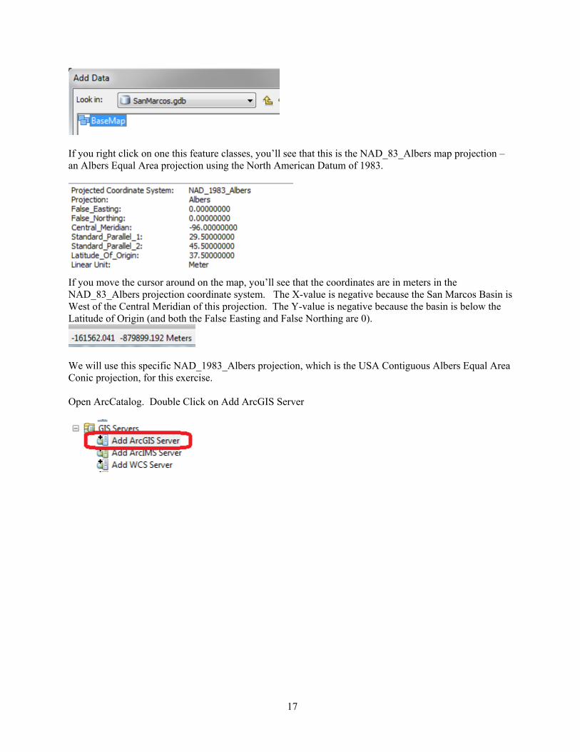
If you right click on one this feature classes, you’ll see that this is the NAD_83_Albers map projection – an Albers Equal Area projection using the North American Datum of 1983.

If you move the cursor around on the map, you’ll see that the coordinates are in meters in the NAD_83_Albers projection coordinate system. The X-value is negative because the San Marcos Basin is West of the Central Meridian of this projection. The Y-value is negative because the basin is below the Latitude of Origin (and both the False Easting and False Northing are 0).

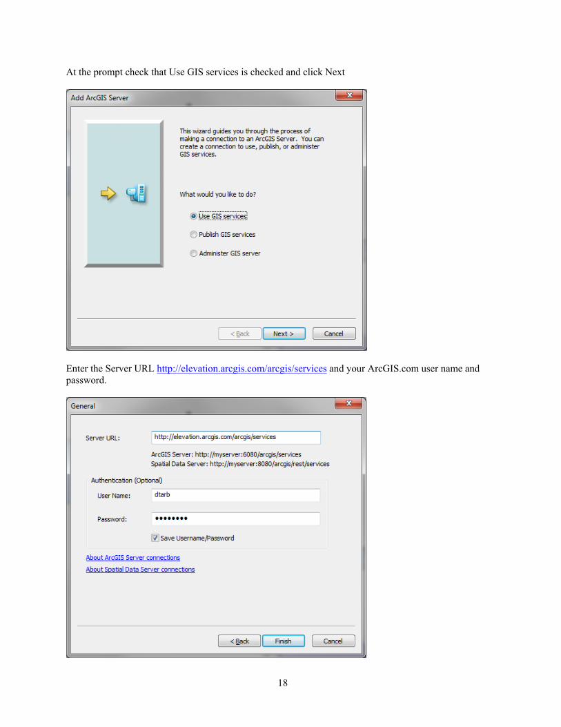
We will use this specific NAD_1983_Albers projection, which is the USA Contiguous Albers Equal Area Conic projection, for this exercise. Open ArcCatalog. Double Click on Add ArcGIS Server

18

At the prompt check that Use GIS services is checked and click Next

Enter the Server URL http://elevation.arcgis.com/arcgis/services and your ArcGIS.com user name and password.

19

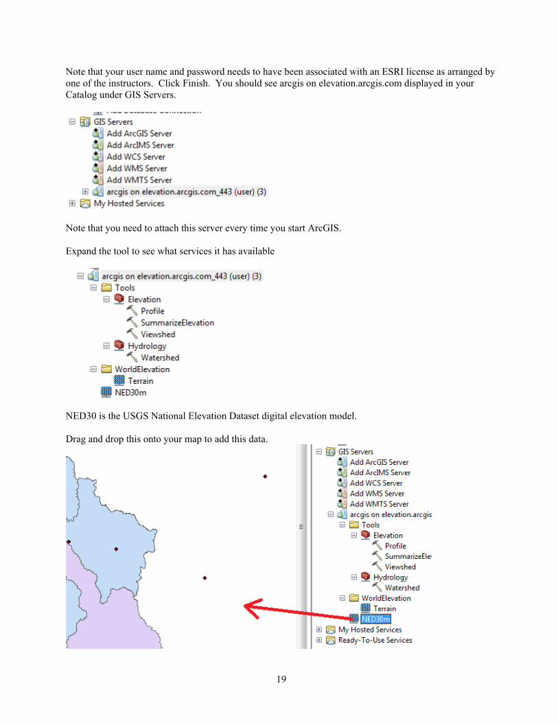
Note that your user name and password needs to have been associated with an ESRI license as arranged by one of the instructors. Click Finish. You should see arcgis on elevation.arcgis.com displayed in your Catalog under GIS Servers.

Note that you need to attach this server every time you start ArcGIS. Expand the tool to see what services it has available

NED30 is the USGS National Elevation Dataset digital elevation model. Drag and drop this onto your map to add this data.

20

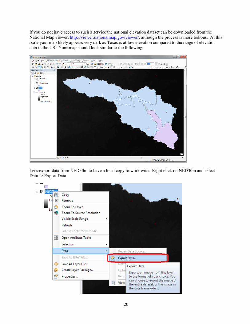
If you do not have access to such a service the national elevation dataset can be downloaded from the National Map viewer, http://viewer.nationalmap.gov/viewer/, although the process is more tedious. At this scale your map likely appears very dark as Texas is at low elevation compared to the range of elevation data in the US. Your map should look similar to the following:

Let's export data from NED30m to have a local copy to work with. Right click on NED30m and select Data -> Export Data

21

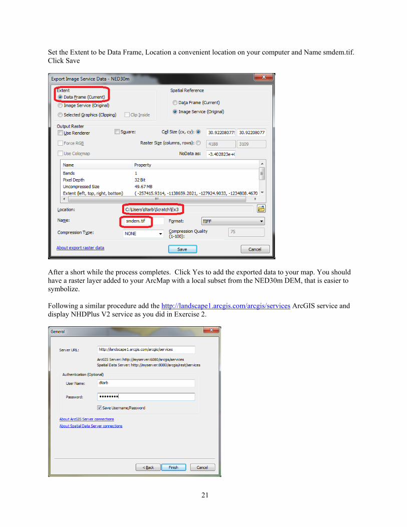
Set the Extent to be Data Frame, Location a convenient location on your computer and Name smdem.tif. Click Save

After a short while the process completes. Click Yes to add the exported data to your map. You should have a raster layer added to your ArcMap with a local subset from the NED30m DEM, that is easier to symbolize. Following a similar procedure add the http://landscape1.arcgis.com/arcgis/services ArcGIS service and display NHDPlus V2 service as you did in Exercise 2.

22

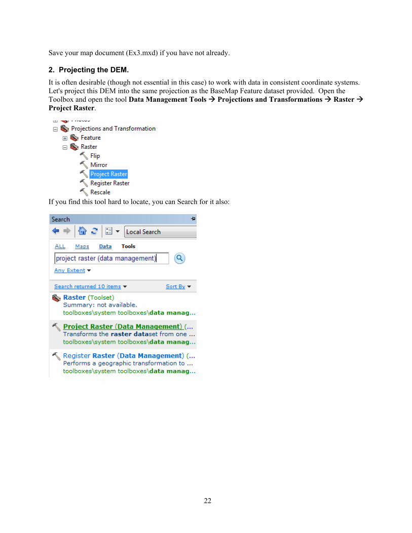
Save your map document (Ex3.mxd) if you have not already. 2. Projecting the DEM.

It is often desirable (though not essential in this case) to work with data in consistent coordinate systems. Let's project this DEM into the same projection as the BaseMap Feature dataset provided. Open the Toolbox and open the tool Data Management Tools Projections and Transformations Raster Project Raster.

If you find this tool hard to locate, you can Search for it also:

23

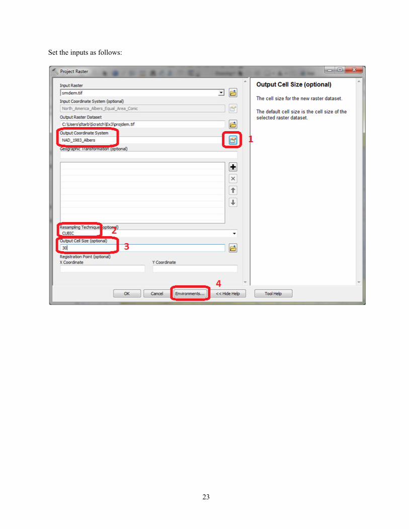
Set the inputs as follows:

24

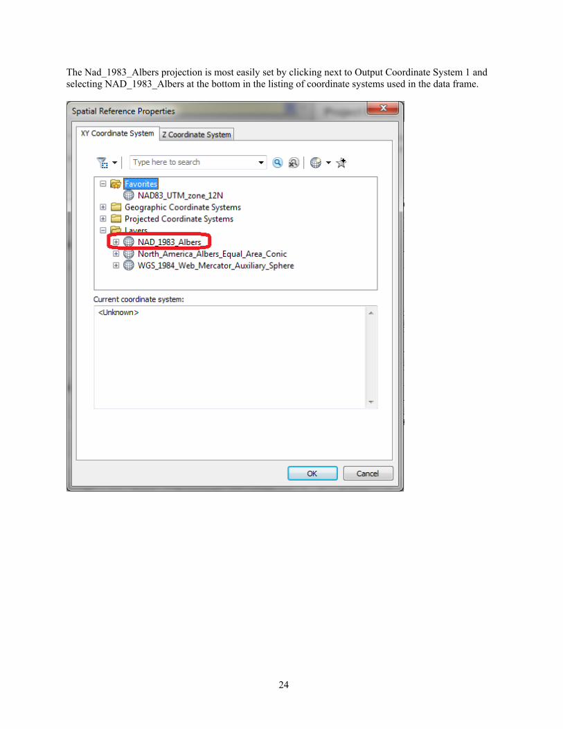
The Nad_1983_Albers projection is most easily set by clicking next to Output Coordinate System 1 and selecting NAD_1983_Albers at the bottom in the listing of coordinate systems used in the data frame.

25

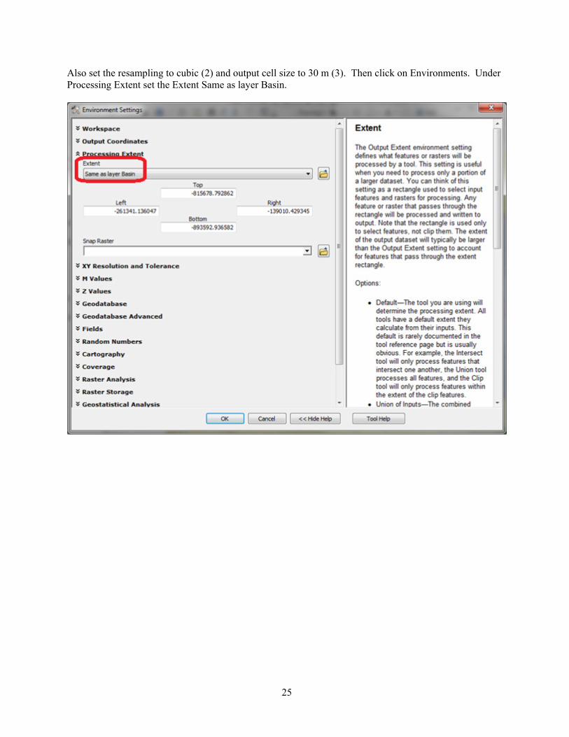
Also set the resampling to cubic (2) and output cell size to 30 m (3). Then click on Environments. Under Processing Extent set the Extent Same as layer Basin.

26

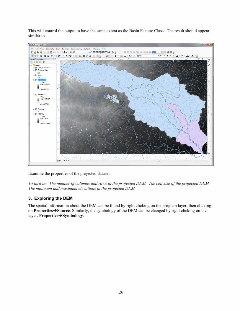
This will control the output to have the same extent as the Basin Feature Class. The result should appear similar to

Examine the properties of the projected dataset. To turn in: The number of columns and rows in the projected DEM. The cell size of the projected DEM. The minimum and maximum elevations in the projected DEM. 3. Exploring the DEM

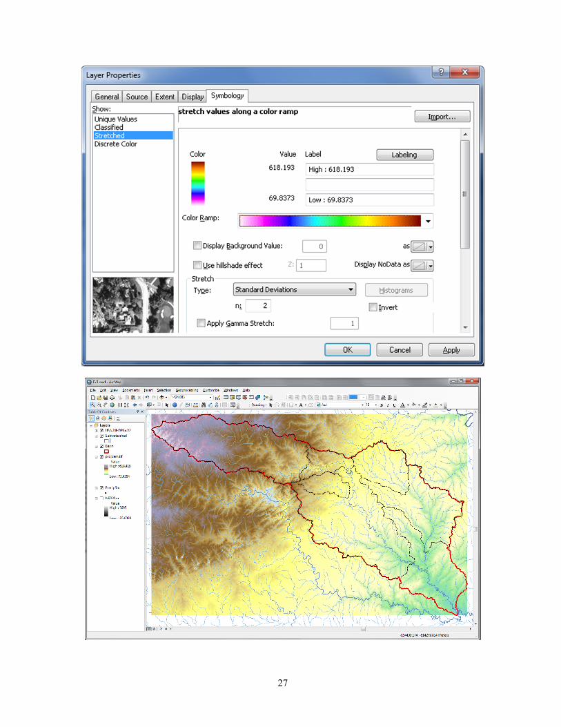
The spatial information about the DEM can be found by right clicking on the projdem layer, then clicking on PropertiesSource. Similarly, the symbology of the DEM can be changed by right clicking on the layer, PropertiesSymbology.

27

28

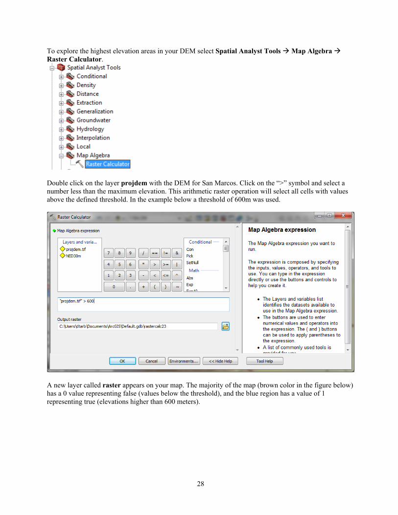
To explore the highest elevation areas in your DEM select Spatial Analyst Tools Map Algebra Raster Calculator.

Double click on the layer projdem with the DEM for San Marcos. Click on the “>” symbol and select a number less than the maximum elevation. This arithmetic raster operation will select all cells with values above the defined threshold. In the example below a threshold of 600m was used.

A new layer called raster appears on your map. The majority of the map (brown color in the figure below) has a 0 value representing false (values below the threshold), and the blue region has a value of 1 representing true (elevations higher than 600 meters).

29

Zoom in to the region of highest elevations and do some sampling on the smdem grid using the identify

tool or pixel inspector to identify the grid cell of maximum elevation. Use the draw tools to mark your point of maximum elevation and label it with the elevation value for that pixel.

To turn in: A layout showing the location of the highest elevation value in the San Marcos DEM. Include a scale bar and north arrow in the layout. 4. Contours and Hillshade

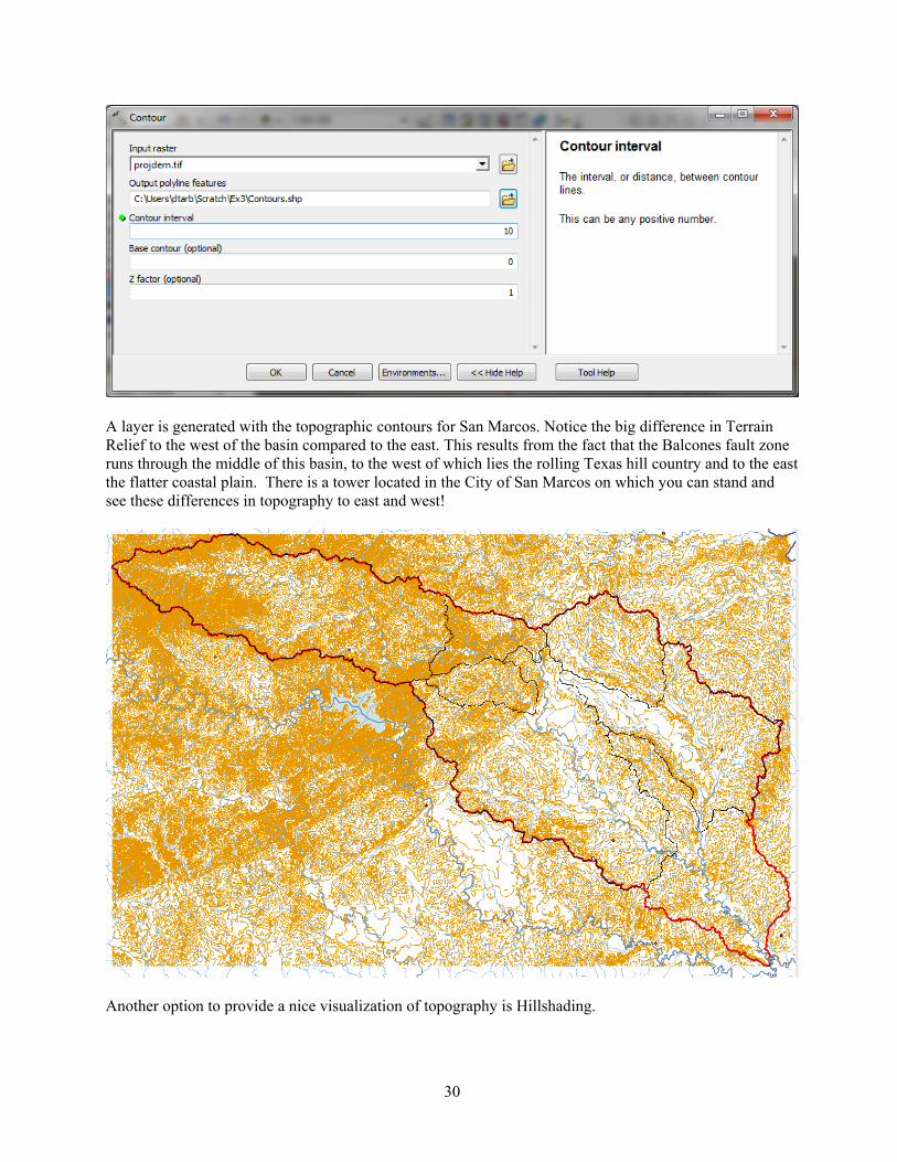
Contours are a useful way to visualize topography. Select Spatial Analyst Tools Surface Contour. Select the inputs as follows, with a 10m contour interval:

30

A layer is generated with the topographic contours for San Marcos. Notice the big difference in Terrain Relief to the west of the basin compared to the east. This results from the fact that the Balcones fault zone runs through the middle of this basin, to the west of which lies the rolling Texas hill country and to the east the flatter coastal plain. There is a tower located in the City of San Marcos on which you can stand and see these differences in topography to east and west!

Another option to provide a nice visualization of topography is Hillshading.

31

Select Spatial Analyst Tools Surface Hillshade and set the factor Z to a higher value to get a dramatic effect and leave the other parameters at their defaults (the following hillshade is produced with a Z factor of 10). Click OK. You should see an illuminated hillshaded view of the topography.

To turn in: A layout with a depiction of topography either with elevation, contour or hillshade in nice colors. Include the streams from the NHDPlus Service and Basin and sub-watersheds from the SanMarcos.gdb Basemap feature dataset.

32

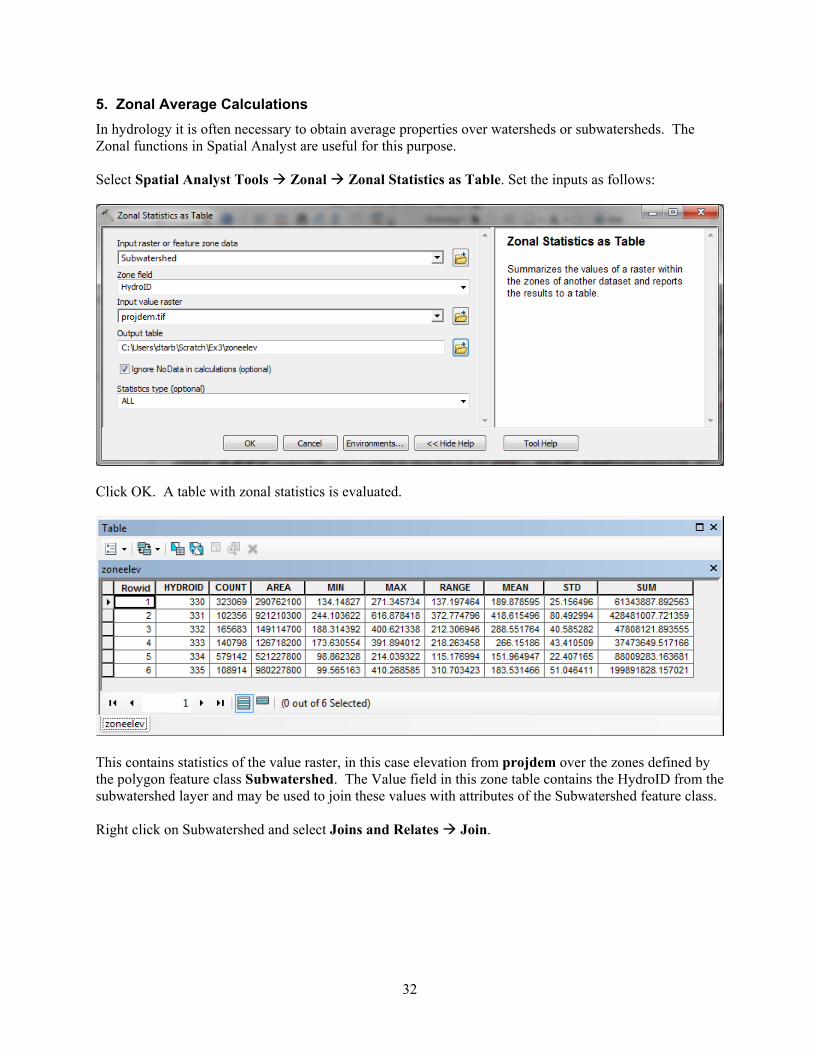
5. Zonal Average Calculations

In hydrology it is often necessary to obtain average properties over watersheds or subwatersheds. The Zonal functions in Spatial Analyst are useful for this purpose. Select Spatial Analyst Tools Zonal Zonal Statistics as Table. Set the inputs as follows:

Click OK. A table with zonal statistics is evaluated.

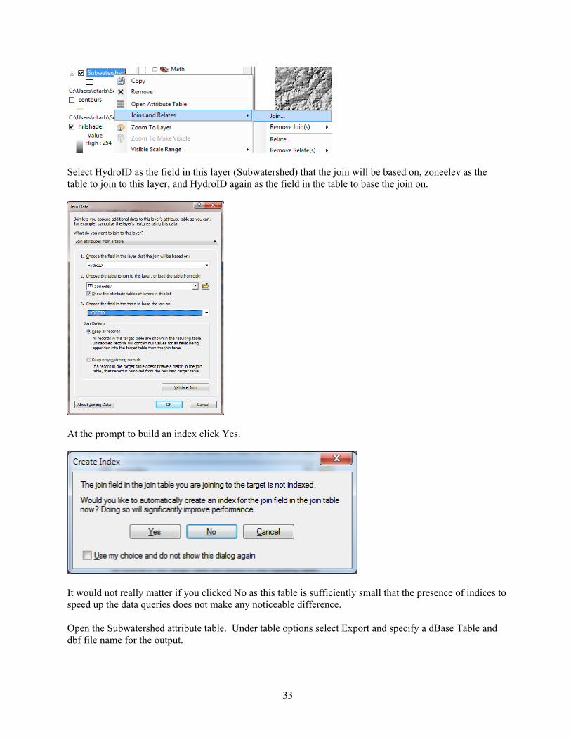
This contains statistics of the value raster, in this case elevation from projdem over the zones defined by the polygon feature class Subwatershed. The Value field in this zone table contains the HydroID from the subwatershed layer and may be used to join these values with attributes of the Subwatershed feature class. Right click on Subwatershed and select Joins and Relates Join.

33

Select HydroID as the field in this layer (Subwatershed) that the join will be based on, zoneelev as the table to join to this layer, and HydroID again as the field in the table to base the join on.

At the prompt to build an index click Yes.

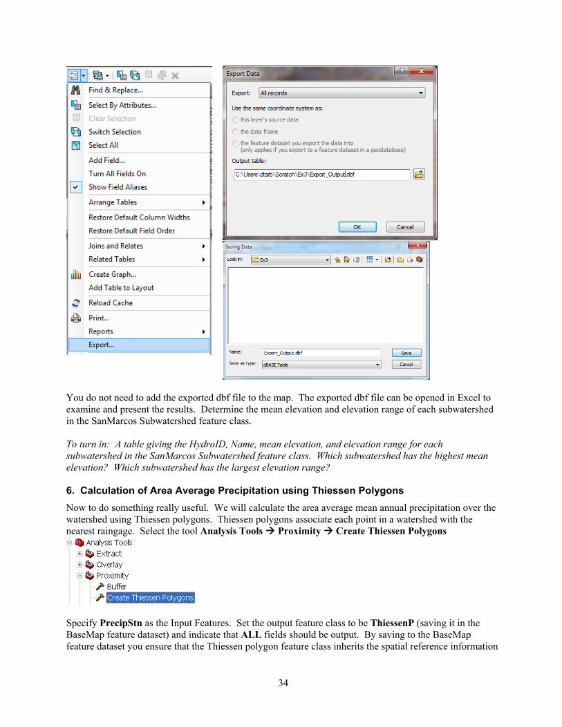
It would not really matter if you clicked No as this table is sufficiently small that the presence of indices to speed up the data queries does not make any noticeable difference. Open the Subwatershed attribute table. Under table options select Export and specify a dBase Table and dbf file name for the output.

34

You do not need to add the exported dbf file to the map. The exported dbf file can be opened in Excel to examine and present the results. Determine the mean elevation and elevation range of each subwatershed in the SanMarcos Subwatershed feature class. To turn in: A table giving the HydroID, Name, mean elevation, and elevation range for each subwatershed in the SanMarcos Subwatershed feature class. Which subwatershed has the highest mean elevation? Which subwatershed has the largest elevation range? 6. Calculation of Area Average Precipitation using Thiessen Polygons

Now to do something really useful. We will calculate the area average mean annual precipitation over the watershed using Thiessen polygons. Thiessen polygons associate each point in a watershed with the nearest raingage. Select the tool Analysis Tools Proximity Create Thiessen Polygons

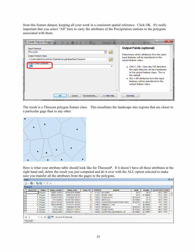
Specify PrecipStn as the Input Features. Set the output feature class to be ThiessenP (saving it in the BaseMap feature dataset) and indicate that ALL fields should be output. By saving to the BaseMap feature dataset you ensure that the Thiessen polygon feature class inherits the spatial reference information

35

from this feature dataset, keeping all your work in a consistent spatial reference. Click OK. It's really important that you select “All” here to carry the attributes of the Precipitation stations to the polygons associated with them.

The result is a Thiessen polygon feature class. This tessellates the landscape into regions that are closer to a particular gage than to any other.

Here is what your attribute table should look like for ThiessenP. If it doesn’t have all these attributes at the right hand end, delete the result you just computed and do it over with the ALL option selected to make sure you transfer all the attributes from the gages to the polygons.

36

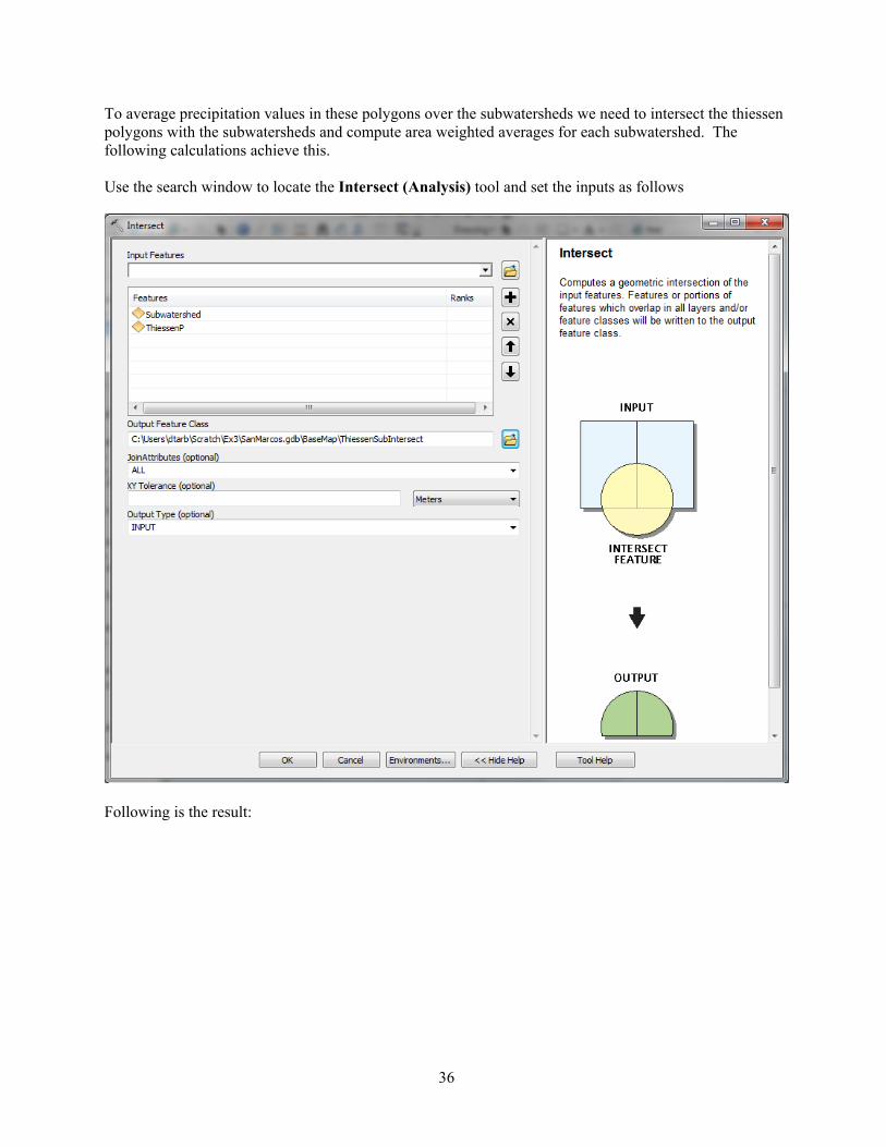
To average precipitation values in these polygons over the subwatersheds we need to intersect the thiessen polygons with the subwatersheds and compute area weighted averages for each subwatershed. The following calculations achieve this. Use the search window to locate the Intersect (Analysis) tool and set the inputs as follows

Following is the result:

37

If you open the ThiessenSubIntersect attributed table you will see that from the 6 subwatersheds there are now 24 polygons, each contributing to part of a subwatershed and associated with a single rain gage. Let Pk denote the precipitation associated with each rain gage and Aik the area of intersected polygon associated with rain gage k and subwatershed i. Then the area weighted precipitation associated with each subwatershed is = ∑∑

Open the attribute table for ThiessenSubIntersect by right clicking on the Table of Contents for it

Add a new field to the table (named APProd)

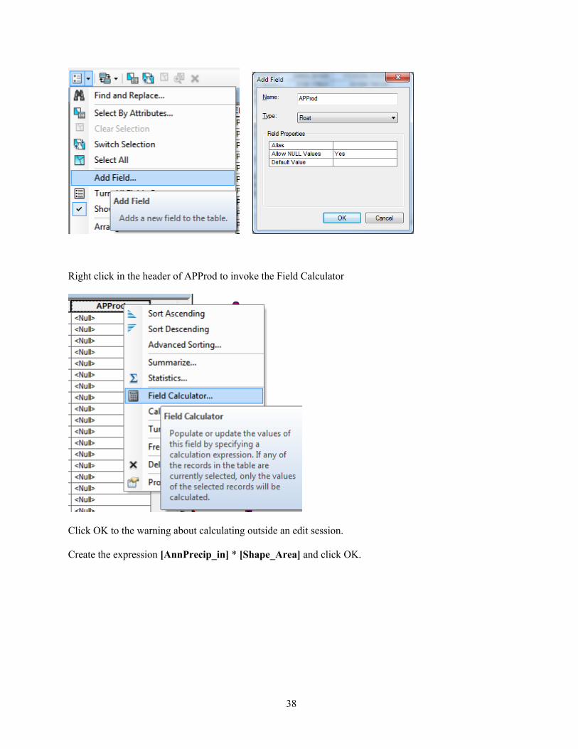
38

Right click in the header of APProd to invoke the Field Calculator

Click OK to the warning about calculating outside an edit session. Create the expression [AnnPrecip_in] * [Shape_Area] and click OK.

39

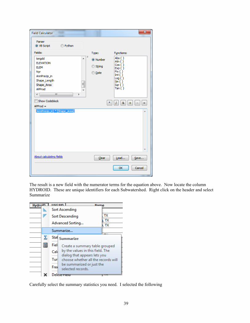
The result is a new field with the numerator terms for the equation above. Now locate the column HYDROID. These are unique identifiers for each Subwatershed. Right click on the header and select Summarize

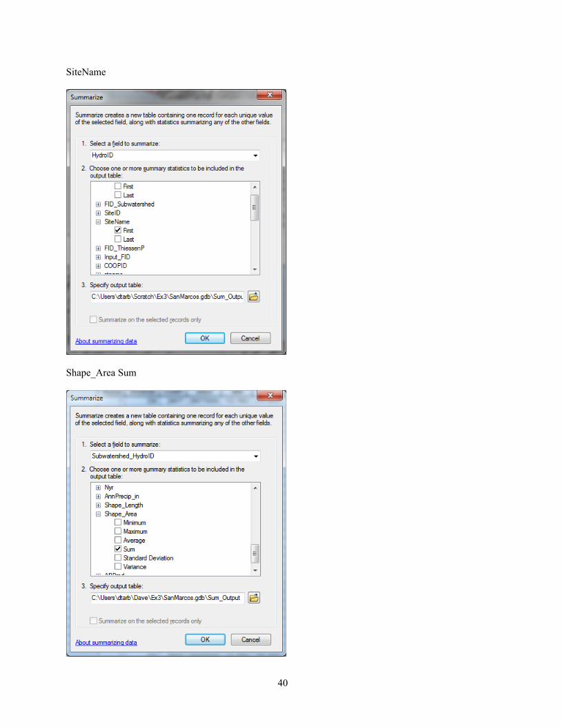
Carefully select the summary statistics you need. I selected the following

40

SiteName

Shape_Area Sum

41

APProd Sum

The resulting table gives the numerator and denominator in the equation above for each subwatershed

42

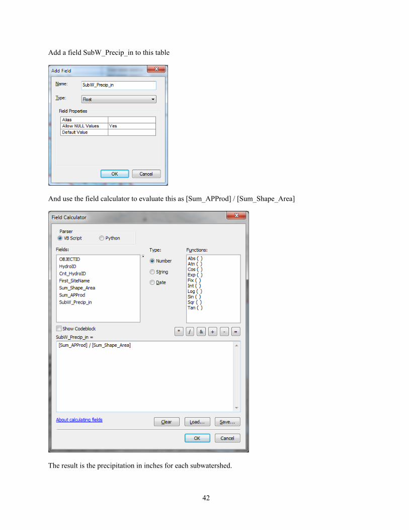
Add a field SubW_Precip_in to this table

And use the field calculator to evaluate this as [Sum_APProd] / [Sum_Shape_Area]

The result is the precipitation in inches for each subwatershed.

43

To turn in: A table giving the HydroID, Name, and mean precipitation by the Thiessen method for each subwatershed in the SanMarcos Subwatershed feature class. Which subwatershed has the highest mean precipitation? 7. Estimate basin average mean annual precipitation using Spatial Interpolation/Surface fitting.

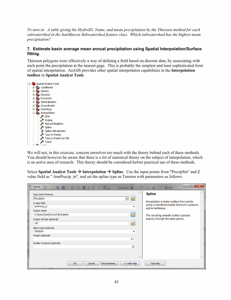
Thiessen polygons were effectively a way of defining a field based on discrete data, by associating with each point the precipitation at the nearest gage. This is probably the simplest and least sophisticated form of spatial interpolation. ArcGIS provides other spatial interpolation capabilities in the Interpolation toolbox in Spatial Analyst Tools.

We will not, in this exercise, concern ourselves too much with the theory behind each of these methods. You should however be aware that there is a lot of statistical theory on the subject of interpolation, which is an active area of research. This theory should be considered before practical use of these methods. Select Spatial Analyst Tools Interpolation Spline. Use the input points from "PrecipStn" and Z value field as " AnnPrecip_in", and set the spline type as Tension with parameters as follows:

44

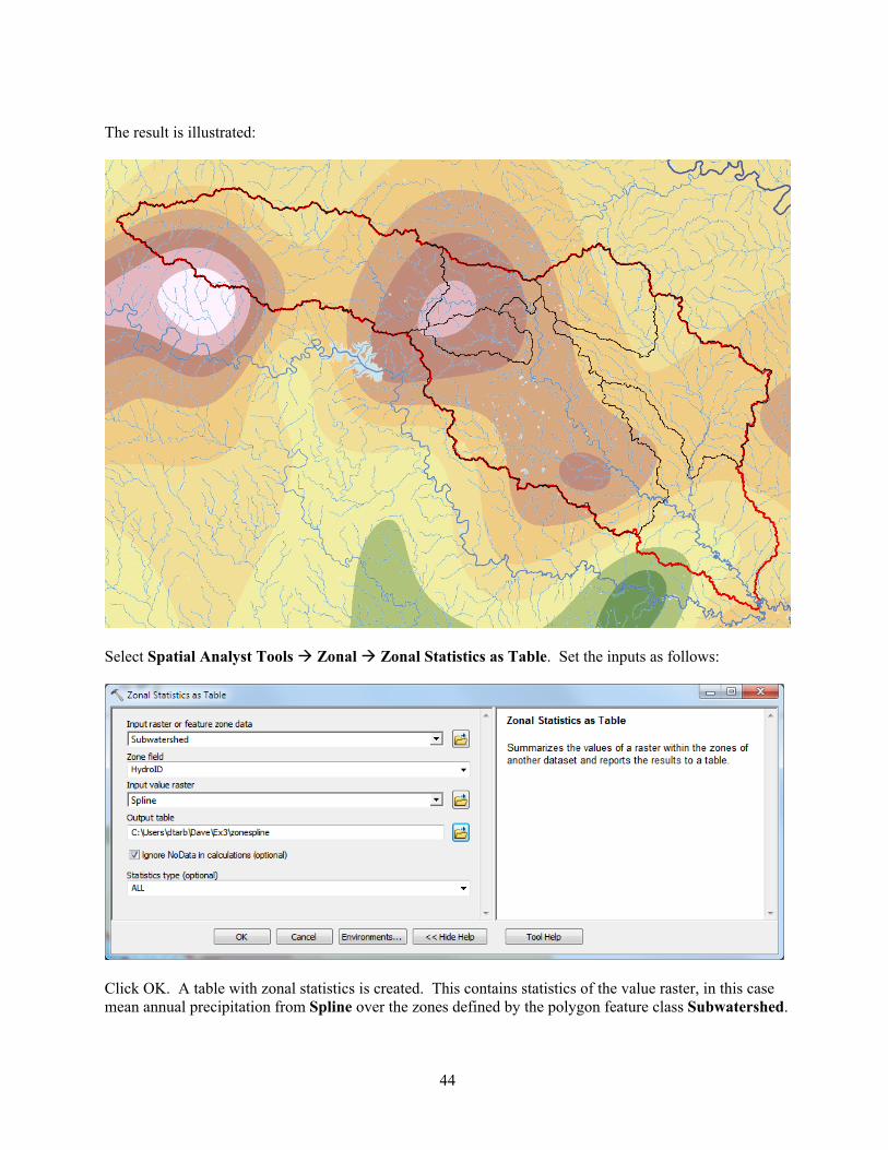
The result is illustrated:

Select Spatial Analyst Tools Zonal Zonal Statistics as Table. Set the inputs as follows:

Click OK. A table with zonal statistics is created. This contains statistics of the value raster, in this case mean annual precipitation from Spline over the zones defined by the polygon feature class Subwatershed.

45

The HydroID in this table may be used to join it to the attribute table for the Subwatershed feature class. As for the elevations above this joined table can be exported and examined and presented in Excel. To turn in: A table giving the HydroID, Name, and mean precipitation by the Tension Spline method for each subwatershed in the SanMarcos Subwatershed feature class. Which subwatershed has the highest mean precipitation using a Tension Spline interpolation? 8. Runoff Coefficients.

Runoff ratio, defined as the fraction of precipitation that becomes streamflow at a subbasin outlet is a useful measure in quantifying the hydrology of a watershed. Mathematically runoff ratio is defined as

w = Q/P where Q is streamflow, and P is precipitation. In this formula, P and Q need to be in consistent units such as depth per unit area or volume. The MAflow field in the Gages point feature class gives the average streamflow at six stream gauges in the San Marcos watershed in ft3/s. To convert these to volume units (say ft3) they should be multiplied by the number of seconds in a year (60 x 60 x 24 x 365.25). In the current exercise mean annual precipitation has been evaluated for each subwatershed, in inches. To convert these to volume units (say ft3) these quantities should be multiplied by 1/12 ft in-1 and multiplied by the subwatershed area in ft2. The subwatershed feature class includes subwatershed area, in the units of the spatial reference frame being used, which are m2. (Remember, 1 ft = 0.3048 m). The necessary calculations are most easily performed in Excel. Use the Options/Export function to export the subwatershed featureclass attribute table that includes your Thiessen basin average subwatershed precipitation results to dbf format that can be read by Excel, as was done above. Similarly export the Gages Point featureclass attribute table that includes mean annual streamflow at each monitoring point. In Excel multiply gage streamflow by 60 x 60 x 24 x 365.25 to obtain streamflow volume, Q, in ft3. Multiply subwatershed average precipitation (in inches) by subwatershed area (in m2)/(12 x 0.30482) to obtain subwatershed precipitation volume, P, in ft3. On the maps you have that show subwatersheds and streams identify the subwatersheds upstream of each gauge. Do this visually by looking at the Flowlines. Add up the precipitation volumes over these subwatersheds then divide Q/P to obtain an estimate of runoff ratio for the watershed upstream of each stream gage. To turn in. A table giving runoff ratio for the watershed upstream of each stream gage.

Summary of Items to turn in: 1. Hand calculations of slope at point A using each of the two methods and comments on the differences. 2. Table giving slope, aspect, hydrologic slope and flow direction at grid cells A and B. Please turn in a diagram or sketch that defines or indicates what each of these numbers means for the specific values obtained for cells A and B. 3. A screen capture of your final model builder model. 4. A table giving the minimum and maximum values of each of the four outputs Slope, Aspect, Flow Direction, and Hydrologic Slope (Percentage drop), for the digital elevation model in demo.asc. 5. The number of columns and rows in the projected DEM. The cell size of the projected DEM. The minimum and maximum elevations in the projected DEM.

46

6. A layout showing the location of the highest elevation value in the San Marcos DEM. Include a scale bar and north arrow in the layout. 7. A layout with a depiction of topography either with elevation, contour or hillshade in nice colors. Include the streams from the NHDPlus Service and Basin and sub-watersheds from the SanMarcos.gdb Basemap feature dataset. 8. A table giving the HydroID, Name, mean elevation, and elevation range for each subwatershed in the SanMarcos Subwatershed feature class. Which subwatershed has the highest mean elevation? Which subwatershed has the largest elevation range? 9. A table giving the HydroID, Name, and mean precipitation by the Thiessen method for each subwatershed in the SanMarcos Subwatershed feature class. Which subwatershed has the highest mean precipitation? 10. A table giving the HydroID, Name, and mean precipitation by the Tension Spline method for each subwatershed in the SanMarcos Subwatershed feature class. Which subwatershed has the highest mean precipitation using a Tension Spline interpolation? 11. A table giving runoff ratio for the watershed upstream of each stream gage.